BUREAU OF THE CENSUS

STATISTICAL RESEARCH DIVISION REPORT SERIES

SRD Research Report Number: CENSUS/SRD/RR-88112

THE DIFFICULTY OF IMPROVING STATISTICAL

SYNTHETIC ESTIMATION

*Michael Lee Cohen and **Xiao Di Zhang University of Maryland Bureau of the Census and Bureau of the Census ASA/Census Program ASA/Census Program Washington, D.C. 20233 Washington, D.C.

*ASA/Census Fellow **ASA/Census Associate

This series contains research reports, written by or in cooperation with staff members of the Statistical Research Division, whose content may be of interest to the general statistical research community. The views re- flected in these reports are not necessarily those of the Census Bureau nor do they necessarily represent Census Bureau statistical policy or prac- tice. Inquiries may be addressed to the author(s) or the SRD Report Series Coordinator, Statistical Research Division, Bureau of the Census, Washington, D.C. 20233.

Recommended by: Kirk M. Wolter

Report completed: March, 1988

Report issued: March 8, I988

The Difficulty of Improving Statistical Synthetic Estimation

Michael Lee Cohen . University of Maryland and Bureau of the Census

and

Xiao Di Zhang Bureau of the Census

Abstract: Statistical synthetic estimation, a technique widely suggested as a method for carrying down estimates to local levels can be shown to be a member of more general classes of estimators. It would then

w seem to follow that, by using information in the data, there,would exist estimators that could select members of these classes based on this information, and that these estimators would outperform

e statistical synthetic estimation. We argue that these estimators are sometimes unavailable, and if they were available, would provide only modest improvements over the performance of the statistical synthetic estimator.

. -2-

1. Definition of Statistical Synthetic Estimator

Assume we have a parent region composed of n subregions. We are provided

with the census counts Xi, i=l ,***, n, for each of the subregions and the

census count X and the true count U, for the parent region, where y x. = x. j-l1 !

Let ui represent the unobserved true counts for the n subregions.

The problem is to estimate the ui under the constraint of internal

consistency, i.e., where the estimates for the subregions sum to U. This

property is important in census applications where it is expected that .

population counts for subregions add to population counts for parent

regionsa In this first case where we have no disaggregation for demographic

subgroups, the statistical synthetic estimate is defined by:

(1) ji = (U/X) xi .

Now assume that we are provided with the census counts disaggregated

demographically. Let US denote Xij as the census count in the i-th subregion

for the j-th demographic subgroup and we have that Xi = i

JIxij

j=l xij . Also let

Xj = be the census count of the parent region for the j-th demographic

subgroup, and let Uj be the true count of the parent region for the j-th

demographic subgroup. Let Uj be assumed known. In this case, the procedure

is to separately apply the computation given above for each demographic

subgroup and then add the results to arrive at the estimate:

(2) 9 * = jql(uj/xj) X.. 1J

-3-

It is clear that these estimates satisfy the constraint of internal

consistency, i.e., that the estimates for a subregion add to the true count U

for the pare@ region (where by the true count we might in practice intend

only an improved count).

This allocation problem was examined by Deming (1938) with the following

situation as motivation. Three measurements are taken of the three interior

angles of a traingle. The three measurements will undoubtedly not add to

180°, and therefore need to be adjusted to incorporate this knowledge into the

esdimates. The methods Deming used are extended here to examine more general

situations'.

I

There are other situations which require internal consistency. One

example arises if one asks respondents to supply probabilities for mutually

exclusive and exhaustive events. Often, due to mistakes, the probabilities

supplied will not sum to 100%. Without recontacting the respondent how should

the observed percentages be modified so that they have the required property?

2. The Model for Statistical Synthetic Estimation

A. The case aggregated by demographic group -- the l-dimensional case.

There are two simple models which result in statistical synthetic

estimation in the l-dimensional case. First, if we restrict ourselves

to estimates of pi of the form:

0 Pi = KXi ,

-4-

n 0 and if we require that 7 ui = U , then K must equal U/X , and

igl

pp = (U/X) xi .

Likewise, if we wish to solve the minimization:

min i (Kxi K ill

- ~i)2/xi

(where Xi is playing the role of a variance as well as an observed

. value) we find that K = U/X. In this second model we are fortunate

that the dependence of K on the individual unknown vi is solely

through the known sum U.

Both of these models seem overly simplistic and narrow. It would be

comforting to users of statistical synthetic estimation if it could be

shown to be optimal for a wider class of estimates. We now show this

to be the case. Following Deming (1938), we assume:

(3) ‘i ‘cd* N(ui , c() , i=l,...,n ,

and furthermore we assume that T ui = U is know. ill

The objective is

to estimate the n vi’s from the n Xi 's under the constraint that the

sum of the estimates equals U.

(A difficulty with this model in the census context is that we have

little reason to assume that the Xi are unbiased. The bias does,

-5-

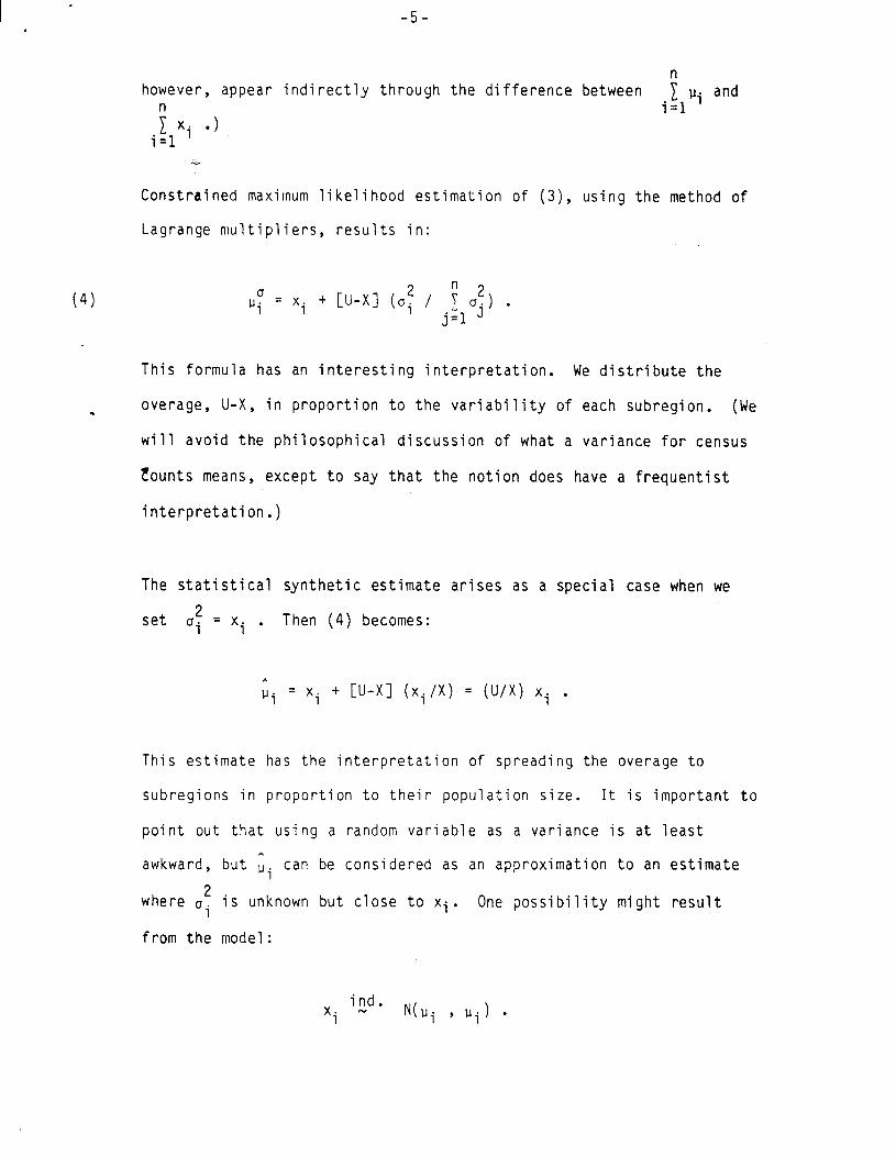
(4)

however, appear indirectly through the difference between

; x. .) i=l

pi and

i=l ' i..

Constrained maximum likelihood estimation of (3), using the method of

Lagrange multipliers, results in:

u Eli i + [U-X] (u:

n 2 = x / z'j)*

j=l

This formula has an interesting interpretation. We distribute the

. overage, U-X, in proportion to the variability of each subregion. (We

will avoid the philosophical discussion of what a variance for census

founts means, except to say that the notion does have a frequentist

interpretation.)

The statistical synthetic estimate arises as a special case when we

set 0: = xi . Then (4) becomes:

ji = xi + [U-X] (Xi/X) = (U/X) x- . 1

This estimate has the interpretation of spreading the overage to

subregions in proportion to their population size. It is important to

point out that using a random variable as a variance is at least

awkward, but j i can be considered as an approximation to an estimate

where o 2 i

is unknown but close to xi. One possibility might result

from the rnodel :

x ind. i- N(ui 9 ui ) l

-6-

.

What this argument shows is that statistical synthetic estimation can

result from a nonparametric model. Also we have now demonstrated .rT

statfstical synthetic estimation as a member of a general class of

estimates (4) which raises the possibility of using members for

specific situations which outperform pi .

B. The case disaggregated by demographic group -- the K-dimensional case.

. The estimate ~7 = ; [U./X.] Xij j=l J J

tesults from constraining a parametric class of estimates (and not

optimizing) as was the case for j i'

Consider the class of estimates:

0 ui = jilKj �ij l

We introduce the constraints that the estimates for demographic

subgroups in subregions should add to the assumed known estimates U. J

for demographic subgroups in the parent region. Thus:

n

C Kj 'ij

i=l = Uj which implies that Kj = Uj/Xj

Nonparametrically, we can derive u 7 from the following generalization

of the l-dimensional case. Let:

ind. 'ij N

N (pij 9 ':j )

-7-

where the 11.. 1J

are unknown means for the

the i-th subregion, and where:

j-th demographic subgroup in

iilpij = Uj , for j=l,...,K.

Just as in the l-dimensional case, a Lagrange multiplier argument can

be used to solve this problem of constrained maximum likelihood,

resulting in:

U

'ij = 'ij + [u.

n 2 J

- ‘jl (‘~j / C U ') m=l ‘J

3. Genzralization of the l-Dimensional Case

We now examine the more general model:

where E' = (xl,...,xn) , k' = (ul 3***aP n) ' and 1 is the nxn covariance matrix

of x . We wish to find the maximum likelihood estimates of ul,...,pn subject

to the constraint i ui = U . i=l

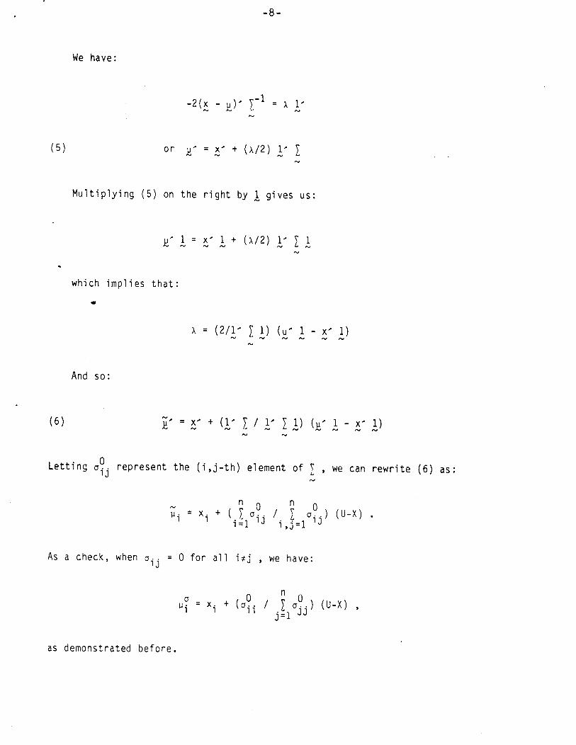
To accomplish this we use Lagrange multipliers. The maximum likelihood

criterion reduces to minimizing:

subject to: k-i-u=o.

-8-

We have:

(5)

-2(x N - !$’ c -1 = x 1' N

or k' = 5' + (x/2) A' 1

Multiplying (5) on the right by i gives us:

which implies that:

And so:

Letting UI represent the (i,j-th) element of 1 , we can rewrite (6) as:

As a check, when aij = 0 for all i#j , we have:

U

pi = x i + i”3i / ~ U”) (U-X) ) j=l JJ

as demonstrated before.

-9-

It is important to mention that in the census application the covariances

'ij are unlikely to be estimable, and it is unclear that even rough estimates

of the u ii

would be available. Thus it would be comforting to know that the

cost of using the wrong weights is often not great.

Consider the case where u.. = 0 for all i#j . Then: 1J

.

Varhy) = E [Xi + (uii / 7

j il"jj

) (U-X) - E h;)12

(7)

Equation (7) makes it clear that the principal objective of statistical

synthetic estimation must be internal consistency, since there is no great

gain in precision. For example, if the variances for the n subregions are

roughly comparable, we have:

Var(py} = "iii{1 - $ = C(n-l)/nl Uii .

Given that it is difficult to beat the census by a large amount, it is

surprising that one can misguess the aii by quite a bit and still outperform

the census. Suppose instead of the uii / y u.. , i-I1 JJ

we use weights fi. Then we

have:

VarI~f} = 'ii C1 - ilfi + f: ( ~ U.. / Uii)] j;l JJ

. -lO-

It is easy to show that Var{$l < Var{Xi) whenever 0 < fi 6 2 crii .

Therefore, if one is able to estimate the variances of the counts for the

subregions within a factor of 2, one can outperform the census counts, but not

by a great deal.

4. Generalization of the K-Dimensional Case

A similar generalization of the K-dimensional case to the generalization

given above for the l-dimensional case could be developed. Instead we follow

a different course. A straightforward approach to take is to choose a loss

function and a parametric form of an estimate, along with the constraints

constra ined optimization imposed by internal consistency, and so

problem: An obvious class of estimates

K

lve the

is:

c Kj x.. . j=1 ‘J

The loss function that is probably proposed most often

Tukey, 1983):

i (a.j - i=l

Ui12 / Ui

in this setting is (see

where ai is some estimate of the population count in the i-th subregion. If

we were to apply all K constraints at once, namely:

iilKj 'ij = Uj for all j ,

we must have that Kj = (Uj/Xj). It is of interest to see what gains are

possible if we use (8) with only one constraint (which would likely not

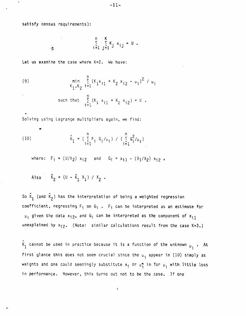
-ll-

satisfy census requirements):

n K

' 5 ☺1 jilKj �ij = � l

Let us examine the case where K=2. We have:

(9) min i (Klxil + K2 xi2 Kl,K2 i=l

such that iiI(Kl Xi1 + K2 Xi2) = U l

.

Solving using Lagrange multipliers again, we find:

I

(10) “i = ( ; F. Gi /Vi ) / ( ? G?/pi ) i=l ' ii1 '

where: Fi = ('J/X2) xi2 and Gi = xi1 - (X1/X2) xi2 ,

Also t2 = (U - R, x1 1 / x2 .

So i, (and K,) has the interpretation of being a weighted regression

coefficient, regressing Fi on Gi . Fi can be interpreted as an estimate for

pi given the data xi2, and Gi can be interpreted as the component of Xi1

unexplained by Xi2. (Note: similar calculations result from the case K=3.)

Kl cannot be used in practice because it is a function of the unknown Pi ' At

first glance this does not seem crucial since the pi appear in (10) simply as

weights and one could seemingly substitute Xi or p: in for 1-1. with little loss 1

in performance. However, this turns out not to be the case. If one

-12-

substitutes Xi for pi in (lo), k1 and I?, turn out to be equal, obviously

rarely optimal. .Furthermore, if one substitutes p; in for pi in (10) il and

k2 turn out to be (U1/X1) and (U,/X,) respectively.

An interesting question is if the pi were available for use as weights, how

much would (10) outperform ~7 . To answer this question we used four

artificial data sets the Bureau of the Census has developed which are believed

to approximate many of the features of undercoverage and which provide a true

count and a census count for subregions and demographic subgroups. These are

fully described in Isaki, Schultz, et al. (1987).

We comprted the estimate in (10) and p 7 for artificial populations II and III,

at the ‘levels of states and counties, for 2 and 3 demographic subgroups. When

we used 2 demographic subgroups Blacks and Hispanics were combined into one

group, otherwise the three demographic subgroups were defined as (i) Blacks,

(ii) Hispanics, and (iii) White and Others. The results are presented in

Table 1.

-13-

Table 1. Comparison of Optimal Estimate with Statistical Synthetic Estimate

Using Artificial Populations - Comparison Made Using Loss Function

1 (ai - l☺i ☺2/vi a l

A. 2 Demographic Groups I = Black + Hispanic II = White + Other

Loss Efficiency of Stat. Synth. Optimal Stat. Synth. Est.

(1) (2)

Estimator (W(2)

Level Data Set State AP2 9754.7 10666.5 .91

AP3 8235.4 9176.5 .90

County AP2 38343.3 39825 .O .96 AP3 39420.8 41384.3 .95

B. 3 Demographic Groups I = Black II = Hispanic III = White + Other .

Loss Efficiency of Stat. Synth. Optimal Stat. Synth. Est. Estimator

1 (1) (2) W/(2) Level Data Set .

State AP2 7847.3 9245.8 .85 AP3 8234.9 9249.7 .89

County AP2 34871.8 36890.9 .95 AP3 39402.6 41564.8 .95

a For K=2, optimal estimate is given in (9). For K=3, similar calculations yield a more complicated expression.

Table 1 indicates that the efficiency of statistical synthetic estimation will

often be very acceptable, especially given that the extra constraints are

likely necessary for the census application of these methods, as well as the

fact that the vi are unknown. The efficiencies are usually above .90. The

difference between AP2 and AP3 is that in AP3 the undercoverage for Hispanics

is assumed to be identical to that for Blacks, while in AP2 the undercoverage

for Hispanics is assumed to be identical to that for Whites and Others. Thus,

it is expected that the AP3 results would be essentially identical for 2 and 3

-14-

demographic groups. Finally, there is a hint that the efficiencies will fall

with a rise in the number of demographic groups used.

5. Conclusion

Statistical synthetic estimation will likely play an important role in

any adjustment of the 1990 Census. It has been suggested as the method by

which estimates derived from the Post-Enumeration Survey will be "carried

down" to small geographic areas. Also, should a timely adjustment be decided

upon (and the Post-Enumeration Survey-based adjustment turns out not to be

timely) statistical synthetic estimation based on national estimates of .

undercoverage derived from demographic analysis could be calculated in time to

meet thp existing statutory deadlines.

We have shown that this simple but important estimator is surprisingly

hardy. In the case for K=l, if one tries to better estimate the weights to

use it is unlikely that the resulting estimator will outperform statistical

synthetic estimaton by much. In the case for K>l, if one relaxes some of the

constraints the defficiency of statistical synthetic estimation is unlikely to

be more than 15%. If one tries to substitute known quantities in as weights

one merely recreates the statistical synthetic estimate or worse. These

results should provide some comfort to prospective users of this methodology.

References

Deming, W. Edwards (1938), "Statisti cal Ad justment of Data," Dover

Publications, Inc., New York.

, -15- .

Isaki, C.T., Schultz, L.K., Smith, P.J.,’ and Diffendal, G.J. (1987), "Small

Area Estimation Research for Census Undercount-Progress Report," pp. 21%

238 in Small Area Statistics: An International Symposium, John Wiley and

Sons, New York, NY.

Tukey, John W. (1983), Affidavit Presented to District Court, Southern

District of New York, Mario Cuomo, et al., Plaintiffs(s), Malcolm Baldrige,

et al., Defendants, 80 CIV. 4550 (JES).

.