Bus Fleet Upgrade Projects

Bus Fleet Upgrade Projects: Discussion of GHG Offsets Methodology Issues

Prepared for: California Climate Action Registry

January 7, 2009

Submitted by:

Science Applications International Corporation

California Climate Action Registry Task Manager: Telephone Number: E-mail:

Rachel Tornek 213-891-6930 rachel@climateregistry.org

SAIC Project Manager: Telephone Number: E-mail:

Jette Findsen (202) 550 8987 findsenj@saic.com

1

Table of Contents

1. Introduction and Summary ......................................................................................................... 1 2. Background – Bus Fleets ............................................................................................................ 4

2.1 Public Transit ........................................................................................................................ 4 2.2 Transit Bus Fuel Types ......................................................................................................... 5 2.3 Energy use and efficiency of transit buses........................................................................... 6 2.4 Other Fleets........................................................................................................................... 8

3. Quantifying Tailpipe and Upstream GHG Emissions ................................................................ 9 3.1 Quantification Methodologies .............................................................................................. 9

4. Datasets and GHG Protocols for Transit Fleets........................................................................ 19 4.1 Datasets on Bus Fleets ........................................................................................................ 19 4.2 Other GHG Project Protocols for Transit Fleets................................................................. 20

5. Performance Standard Development ........................................................................................ 21 5.1 Spatial Categorization......................................................................................................... 24 5.2 Eligibility of All Bus Fuel Types........................................................................................ 27 5.3 Expanding the Performance Standard to Include Other Bus Fleets.................................... 32 5.4 Summary and Implications ................................................................................................. 32

6. Additionality ............................................................................................................................. 33 6.1 Regulatory Additionality .................................................................................................... 33 6.1.1 Federal Requirements ...................................................................................................... 33 6.1.2 State and Local Requirements ......................................................................................... 34 6.2 Voluntary Funding Programs.............................................................................................. 35 6.3 Implementation Barriers ..................................................................................................... 36 6.3.1 Financial Barriers...................................................................................................... 36 6.3.2 Technological Barriers..................................................................................................... 37 6.3.3 Institutional Barriers ........................................................................................................ 38

8. Baseline Quantification............................................................................................................. 38 8.1 Tailpipe Emissions.............................................................................................................. 39 8.2 Upstream Emissions............................................................................................................ 39 8.3 Selecting the Baseline ......................................................................................................... 39

9. Potential Reduction Opportunity .............................................................................................. 41 10. Project Boundary .................................................................................................................... 44

10.1 Primary Effects ............................................................................................................. 44 10.1.1 Assessment Boundary................................................................................................... 44 10.2 Secondary Effects ......................................................................................................... 46 10.2.1 One-Time Effects...................................................................................................... 47 10.2.2 Upstream and Downstream Effects .......................................................................... 47

11. Ownership ............................................................................................................................... 48 12. Scientific Uncertainty ............................................................................................................. 49 13. Other Positive/Negative Environmental, Public Health and Social/Economic Impacts......... 49 14. Market Interest ........................................................................................................................ 51 References..................................................................................................................................... 53

Bus Fleet Upgrade Projects: Discussion of GHG Offsets Methodology Issues

1. Introduction and Summary Topic: Converting technology in bus fleets for cleaner fuels (fuel switch), or upgrading the fleet with hybrid or electric technologies to increase bus fleet efficiency. This paper discusses the key issues with developing a GHG offsets methodology for bus fleet upgrades, including options for setting a performance threshold for identifying those projects that should receive credit. A performance standard sets a threshold emissions level that is significantly better than the average emissions performance for a specified service. In this case, we expect the threshold to be set by reference to the emissions performance of bus fleets. If a project for improving fleet performance has emissions that are equal to or better than the threshold, then the project would be considered to exceed the “business-as-usual” (BAU) performance and would be eligible for registration of emission reduction credits. We begin the report with providing background information on bus fleets and transit buses. The discussion focuses on transit buses because this is where we have the most information, and because prior offsets methodology work is available for this type of buses. However, to the extent possible, we also provide information on other types of fleet with uniform drive cycles and fleet characteristics. We then summarize the GHG accounting issues involved with estimating emission benefits of heavy duty buses, highlighting uncertainties related to estimating CH4 and N2O emission from the tailpipe and to quantifying upstream emissions from alternative fuel vehicles such as biodiesel, electricity, natural gas, hydrogen, and fuel cells. As will be described, these accounting issues have a strong influence on which vehicle types can be included in the performance standard, because they determine which type of metric to use for the threshold. In the discussion of the performance standard, the report expands on the specific issues that need to be considered when developing a threshold for bus fleet projects that increase emissions performance by converting fleets to run on alternative fuels or by upgrading to hybrid or electric engine technologies. For comparison, we utilize the only standardized protocol on related projects currently available in the U.S., the EPA Climate Leaders Protocol for “Transit Bus Efficiency.” EPA’s performance standard focuses on CO2 tailpipe emissions from transit buses and it is only applicable to buses fueled by gasoline, diesel, or oil-based propane. This would include diesel and gasoline hybrid buses. To allow for a comparison across bus fuel types, EPA used a fuel neutral metric of CO2 emissions per miles driven for the performance threshold. There are significant spatial issues that affect the drive cycle and thus emissions performance of transit fleets. EPA accommodated some of these in their methodology, referencing the different driving conditions (e.g., stop-and-go traffic) in larger metropolitan areas versus smaller metropolitan areas, EPA developed separate thresholds for cities with a population of more than

1

one million and less than one million.1 However, the methodology may still exclude some outlier fleets with extremely high stop-and-go traffic, such as those operating in New York City, because those buses would be much less efficient than average fleets in the U.S. This report explores other approaches than the one used by EPA to determine whether there is a better way to reflect geographic differences among fleets and whether it is possible to expand the performance standard beyond oil-based buses to also include natural gas, electric, biofuel, fuel cell, and hydrogen buses. It also examines whether it would be possible to develop performance thresholds for other types of fleets, such as commercial long-haul or school buses. One alternative option we consider is whether the threshold should be set based on individual fleet emission rates, rather than a national emission rate. In this case, the framework for establishing the emissions threshold would be similar to that for establishing a national performance standard, except instead of selecting the threshold emissions rate from the whole range of bus fleets in the U.S., the threshold would be selected from the range of emission performances of all the vehicles within an individual fleet. As will be outlined in the report, some of the considerations in including all potential vehicles in the performance standard and in choosing between a national versus fleet-specific approach include:

- Spatial variations in fleet operations which make the use of a national level threshold less representative of performance by all fleets;

- Limited availability of nationwide data on fleet characteristics; - Challenges in creating a metric for emissions performance that enables comparison

across all types of fuels; and - Lack of established emission factors for estimating upstream emissions from alternative

fuels. As summarized in Table 1, the report finds that expanding the performance standard to include all possible vehicle fuel types would require the inclusion of tailpipe and upstream GHG emission factors in the calculation of the performance threshold. Because of the limited national-level data on fleet activities, this shift would mean that the performance standard should be fleet-specific since this is the only way that the required activity data can be collected. It would also require additional research to select/establish upstream emission factors for all fuels, unless the Registry chooses to exclude fuels with the highest uncertainty such as natural gas, hydrogen, and fuel cells. The advantage of a fleet-specific standard would be the ability of the metric to capture all of the spatial, fleet make-up, operational and maintenance conditions specific to a particular fleet that complicate the application of a single national standard. However, using a fleet-specific approach, the time and reporting burden would shift away from CCAR to the fleet operators.

1 The performance threshold for both large and small metropolitan areas, areas with greater than or less than one million people, respectively, was set at the top 10th percentile of the CO2 per miles driven of the typical transit bus emission rate in each of the areas. For large metropolitan areas, proposed projects have to meet or exceed 2.11 kg CO2 per mile; for small areas, they have to meet or exceed 1.46 kg CO2 per mile.

2

This would conflict with one of the goals of the standardized offsets approach which is to relieve the upfront costs to the project developer of preparing offsets projects. Table 1: Outline of the Considerations Relevant to Setting a Fleet Upgrade Performance Standard for GHG Offsets Projects

Fuel Issue

Conventional Fuels

Diesel-Electric Hybrid

Natural Gas Biofuels Fuel Cell and Plug-In

National Standard

Fleet-Specific Standard

Upstream GHG Quantification

- Relatively well understood and uniformly efficient for U.S. supply

- Same as for diesel

- Many uncertainties related to production sources, processing energy types and distribution efficiencies

- Accounting of indirect impacts highly uncertain - Increasing variability in market sources

- Energy source more variable, but likely traceable - Electricity factors well established

- Emissions for supply may differ significantly within some fuel types and sources - Emission factors not well established except for electricity

- Some sources hard to trace - Emission factors not well established except for electricity

Tailpipe GHG Quantification

- Well established accounting methods

- Well established accounting methods

- CH4 and N2O emissions highly variable by engine/vehicle and driving conditions. Requires vehicle-specific factors

- Mostly CO2, accounting similar to conventional fuels - Accuracy of N2O accounting more of a concern

- Zero GHG emissions

- Aggregate data cannot support quantification of CH4 and N2O

- Fleet data on miles driven by fuel type supports quantification of CH4 and N2O

CO2

- Carbon content values well-established

- Carbon content values well-established

- Carbon content values well-established

- Requires separation of C from renewable and non-renewable sources

- Depends on upstream fuel source

- Expression per mile driven is standard and possible with acceptable national comparability

- Specificity allows accounting for fuel supply C differential

CH4

- General uncertainty of emission factors

- General uncertainty of emission factors

CH4 may outweigh CO2 savings, depends on vehicle, driving

- General uncertainty of emission factors

- Depends on upstream fuel source

- No national datasets available to estimate emissions

- Fleet activity data supports estimation of emissions

N2O

- General uncertainty of emission factors

- May be higher for some biofuels than diesel

- Depends on upstream fuel source

- No national datasets available to estimate emissions

- Fleet activity data supports estimation of emissions

- Fuel economy and emissions vary with

- Very high spatial variability of

- Upstream emissions highly

- Upstream emissions somewhat

- Does not capture spatial variables well

- Captures spatial variables

3

Fuel Issue

Conventional Fuels

Diesel-Electric Hybrid

Natural Gas Biofuels Fuel Cell and Plug-In

National Fleet-Standard Specific

Standard Spatial Variables

driving – idling, stop/start, grade, load all important determinants

GHG emissions

variable geographically

locally variable

2. Background – Bus Fleets Across the U.S., thousands of public and private entities operate fleets of a handful to thousands of buses. The largest fleets are operated by local public transit agencies, school districts, commercial long-haul bus transportation companies (e.g., Greyhound), and charter or tour bus agencies. In some cases, transit agencies and school districts may contract all or part of their operations or routes to private operators. While each of these types of fleets operate on regular routes, this paper focuses on public transit bus fleets due to the availability of the data necessary for analyzing offset project suitability and project-related greenhouse gas reductions, and a history of similar offset project methodologies that have already been developed for this type of buses. 2.1 Public Transit Buses represent the dominant choice of public transportation in the U.S. and the rest of the world, both in terms of the amount of air pollution and greenhouse gases (GHGs) emitted and the total number of passengers, vehicles, and distance traveled. In many areas, buses are the only public transportation choice available.2 In the U.S., 1,500 agencies operate transit buses, representing 83,080 active vehicles.3 These vehicles travel about 2.5 billion total vehicle miles annually, with an average trip taken of 3.9 miles, an average 30,030 miles driven per vehicle per year, and an average speed in revenue service of 12.6 mph. The transit bus classification covers buses transporting passengers through urban and suburban street networks. Most buses have two doors, one in the front and one in the center, and the engine is normally rear-mounted. U.S. transit buses also include smaller varieties with one-door, and larger articulated buses. Generally, bus models are matched to specific routes, types of operation, and demand levels, although the selection is not always optimal. Although transit bus fleets and operations are diverse and tailored to the needs of the communities they serve, there are common characteristics among fleets operating in geographic areas with similar populations. Transit buses normally drive in standard routes with regular stops and are normally parked, maintained, and refueled at centrally located depots allowing for central tracking of fuel consumption, miles driven, and passengers transported. 2 Sigurd Grava, Urban Transportation Systems. Choices for Communities. McGraw-Hill: New York, 2003, p.301. 3 American Public Transportation Association (APTA), Bus and Trolleybus National Totals Fiscal Year 2006, Table 51. http://www.apta.com/research/stats/factbook/documents08/2008_bus_tb_mode_final.pdf.

4

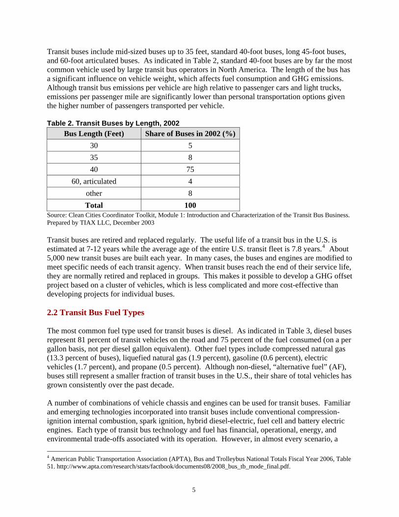
Transit buses include mid-sized buses up to 35 feet, standard 40-foot buses, long 45-foot buses, and 60-foot articulated buses. As indicated in Table 2, standard 40-foot buses are by far the most common vehicle used by large transit bus operators in North America. The length of the bus has a significant influence on vehicle weight, which affects fuel consumption and GHG emissions. Although transit bus emissions per vehicle are high relative to passenger cars and light trucks, emissions per passenger mile are significantly lower than personal transportation options given the higher number of passengers transported per vehicle. Table 2. Transit Buses by Length, 2002

Bus Length (Feet) Share of Buses in 2002 (%) 30 5 35 8 40 75

60, articulated 4 other 8 Total 100

Source: Clean Cities Coordinator Toolkit, Module 1: Introduction and Characterization of the Transit Bus Business. Prepared by TIAX LLC, December 2003 Transit buses are retired and replaced regularly. The useful life of a transit bus in the U.S. is estimated at 7-12 years while the average age of the entire U.S. transit fleet is 7.8 years.4 About 5,000 new transit buses are built each year. In many cases, the buses and engines are modified to meet specific needs of each transit agency. When transit buses reach the end of their service life, they are normally retired and replaced in groups. This makes it possible to develop a GHG offset project based on a cluster of vehicles, which is less complicated and more cost-effective than developing projects for individual buses. 2.2 Transit Bus Fuel Types The most common fuel type used for transit buses is diesel. As indicated in Table 3, diesel buses represent 81 percent of transit vehicles on the road and 75 percent of the fuel consumed (on a per gallon basis, not per diesel gallon equivalent). Other fuel types include compressed natural gas (13.3 percent of buses), liquefied natural gas (1.9 percent), gasoline (0.6 percent), electric vehicles (1.7 percent), and propane (0.5 percent). Although non-diesel, “alternative fuel” (AF), buses still represent a smaller fraction of transit buses in the U.S., their share of total vehicles has grown consistently over the past decade. A number of combinations of vehicle chassis and engines can be used for transit buses. Familiar and emerging technologies incorporated into transit buses include conventional compression-ignition internal combustion, spark ignition, hybrid diesel-electric, fuel cell and battery electric engines. Each type of transit bus technology and fuel has financial, operational, energy, and environmental trade-offs associated with its operation. However, in almost every scenario, a 4 American Public Transportation Association (APTA), Bus and Trolleybus National Totals Fiscal Year 2006, Table 51. http://www.apta.com/research/stats/factbook/documents08/2008_bus_tb_mode_final.pdf.

5

passenger’s choice to ride a transit bus over driving a single occupancy vehicle would reduce fuel consumption and air emissions, including GHGs. Table 3. Number, Power Source, and Efficiency of Transit Buses by Mode

Transit Buses Fuel Consumption Power Source

Number Percent (%)

Thousands of Gallons

Percent (%)

Efficiency – Diesel Gallon Equivalent (Miles per Gallon)

Diesel (including electric hybrid)

44,508 81.4 536,700 74.5 7.05

Clean Diesel (ULSD) 618 1.1

Gasoline 312 0.6 2,300 0.3 4.72

Compressed Natural Gas (CNG)

7,149

13.3 138,800 19.3 2.77

Liquefied Natural Gas (LNG)

1,068 1.9 19,600 2.7 2.19

Methanol 0 0.0 0 0 0.96

Propane 309 0.5 1,600 0.2 1.41

Other (a) 375 1.1 21,400 3.0 N/A

Total Non-Electric 54,339 98.3 720,500 100 N/A

Plug-In Electric 1,022 1.7 70,079 (b) N/A 0.59 (c)

Total 55,361 100 720,500 N/A N/A Source: APTA, 2002. Table 81: Power Source Efficiency, Miles per Gallon; APTA. Bus and Trolleybus Power Sources (2006), Fuel and Power Consumption (2004), http://www.apta.com/research/stats/bus/ (a) Includes bio or soy fuel, biodiesel, jet fuel, and propane blends; (b) KWh; (c) Miles per kilowatt hour.

2.3 Energy use and efficiency of transit buses Most of the primary energy use associated with conventional transit buses occurs during vehicle operation; that is, when the fuel is combusted to power the engines. However, some upstream energy is also used during the production of the vehicles and the production, processing, and transportation of the fuel consumed. Two exceptions are plug-in electric and hydrogen fuel cell buses, in which cases, energy consumption takes place during the upstream production of electricity or hydrogen. During vehicle operation, transit buses consume energy to provide both motive power and to support auxiliary systems. Factors governing the fuel economy of buses are:

6

• Vehicle inertia, influenced by vehicle and passenger weight, or acceleration (kinetic) energy;

• Vehicle drag coefficient, and frontal area and tire rolling resistance; • Accessory requirements, such as air conditioning, compressed air and power steering;

and • Efficiency with which power is transferred to the wheels.

The efficiency of buses will also vary significantly depending on the drive cycle they are operated on, the climate they are driven in, and the specific outfitting of the bus. For example, buses driven with low average speeds and frequent stopping and starting in Manhattan generally will result in much lower efficiencies than buses driven in suburban areas where stops are less frequent and average speeds are higher between stops. In addition, cold climates reduce conventional engine combustion efficiency, while extremely warm climates limit the amount of regenerative braking energy that can be absorbed by the battery packs in electric and hybrid-electric vehicles. These issues are further discussed below with respect to setting a performance standard. The average efficiency of transit buses in the U.S. has increased only slightly over the past decade. As shown in the last column of Table 3 above, diesel engines are much more efficient than any of the alternative fuel-based engines currently available. This is because diesel contains the highest energy density (i.e., the amount of energy per gallon) of available transportation fuels. Moreover, diesel engines operate in a lean (excess air) combustion mode, which provides inherently higher fuel efficiency, and durability in use, and thus performance, over time. Dedicated AF engines, such as those built for exclusive use of compressed or liquefied natural gas (CNG, LNG) or propane, use spark ignition, which provides lower thermal efficiency than do compression ignition diesel engines. For AF transit buses, this may translate into a fuel economy reduction of up to 25 percent per Btu of fuel burned and the need for larger and heavier on-board fuel storage systems.5 Advances in pilot ignition technologies may increase the efficiency of alternative fuel vehicles (AFVs) to near 95% of traditional diesel buses.6 In spite of some of these disadvantages, AFs may result in significantly lower emissions of local air pollutants on a per unit and per mile basis and are increasingly used as a means to reduce local air pollution. As illustrated in Table 4, during combustion alternative fuels also result in lower carbon dioxide emissions (CO2) per unit fuel (i.e., gallon) compared with diesel and gasoline.

5 Clean Cities Coordinator Toolkit, Module 2: Basics of Alternative Fuels in Transit Bus Applications. Prepared by TIAX LLC, December 2003. 6 Mark, J. and C. Morey. 2000. Rolling Smokestacks. Union of Concerned Scientists. p. 24.

7

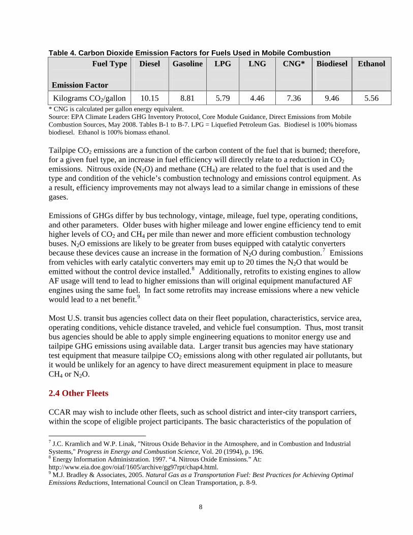
Table 4. Carbon Dioxide Emission Factors for Fuels Used in Mobile Combustion Fuel Type

Emission Factor

Diesel

Gasoline

LPG

LNG

CNG*

Biodiesel

Ethanol

Kilograms CO2/gallon 10.15 8.81 5.79 4.46 7.36 9.46 5.56 * CNG is calculated per gallon energy equivalent. Source: EPA Climate Leaders GHG Inventory Protocol, Core Module Guidance, Direct Emissions from Mobile Combustion Sources, May 2008. Tables B-1 to B-7. LPG = Liquefied Petroleum Gas. Biodiesel is 100% biomass biodiesel. Ethanol is 100% biomass ethanol. Tailpipe CO2 emissions are a function of the carbon content of the fuel that is burned; therefore, for a given fuel type, an increase in fuel efficiency will directly relate to a reduction in CO2 emissions. Nitrous oxide (N2O) and methane (CH4) are related to the fuel that is used and the type and condition of the vehicle’s combustion technology and emissions control equipment. As a result, efficiency improvements may not always lead to a similar change in emissions of these gases. Emissions of GHGs differ by bus technology, vintage, mileage, fuel type, operating conditions, and other parameters. Older buses with higher mileage and lower engine efficiency tend to emit higher levels of CO2 and CH4 per mile than newer and more efficient combustion technology buses. N2O emissions are likely to be greater from buses equipped with catalytic converters because these devices cause an increase in the formation of N2O during combustion.7 Emissions from vehicles with early catalytic converters may emit up to 20 times the N2O that would be emitted without the control device installed.8 Additionally, retrofits to existing engines to allow AF usage will tend to lead to higher emissions than will original equipment manufactured AF engines using the same fuel. In fact some retrofits may increase emissions where a new vehicle would lead to a net benefit.9 Most U.S. transit bus agencies collect data on their fleet population, characteristics, service area, operating conditions, vehicle distance traveled, and vehicle fuel consumption. Thus, most transit bus agencies should be able to apply simple engineering equations to monitor energy use and tailpipe GHG emissions using available data. Larger transit bus agencies may have stationary test equipment that measure tailpipe CO2 emissions along with other regulated air pollutants, but it would be unlikely for an agency to have direct measurement equipment in place to measure CH4 or N2O. 2.4 Other Fleets CCAR may wish to include other fleets, such as school district and inter-city transport carriers, within the scope of eligible project participants. The basic characteristics of the population of

7 J.C. Kramlich and W.P. Linak, "Nitrous Oxide Behavior in the Atmosphere, and in Combustion and Industrial Systems," Progress in Energy and Combustion Science, Vol. 20 (1994), p. 196. 8 Energy Information Administration. 1997. “4. Nitrous Oxide Emissions.” At: http://www.eia.doe.gov/oiaf/1605/archive/gg97rpt/chap4.html. 9 M.J. Bradley & Associates, 2005. Natural Gas as a Transportation Fuel: Best Practices for Achieving Optimal Emissions Reductions, International Council on Clean Transportation, p. 8-9.

8

school buses, fleet ownership and vehicle usage across the U.S. may make this bus sector particularly amenable to offsets project development. There is relative uniformity of vehicle and fuel types among school buses in comparison with the increasing variability in the transit sector. The fleet is dominated by just two bus chassis types and is heavily weighted towards diesel usage.10 Bus Classes C and D accounted for 80% of the fleet in 2004. However, there is no national-level dataset available to describe the specific fleet characteristics and fuel consumption of these individual fleets.

3. Quantifying Tailpipe and Upstream GHG Emissions Mobile source emissions are typically quantified by applying the best-fit emissions factors for CO2, CH4 and N2O to activity data for a particular vehicle. The practice is well established for the quantification of the emissions that occur from the vehicle’s tailpipe, although uncertainty remains regarding the accuracy of the actual CH4 and N2O emission factors applied using these established accounting methods. Upstream emissions in contrast can be defined using a number of different boundaries for the occurrence of indirect effects. The practice of accounting for upstream emissions is thus less uniform and the scientific, environmental, economic and social components of such accounting remain subjects of contentious debate. 3.1 Quantification Methodologies Quantification of tailpipe GHG emissions from bus fleets is relatively straightforward and the accounting conventions are particularly well established for CO2. The use of conventional transportation fuels (e.g., gasoline and diesel) results in emissions of mostly CO2 from the tailpipe. There are sufficient quantification methodologies to develop reliable estimates of potential reductions from projects using these types of fuels. The most accurate method of tracking and comparing tailpipe CO2 emissions is in terms of CO2 per unit fuel used (i.e., gallon). The calculation of tailpipe CH4 or N2O is a bit more complicated. These gases are calculated using emissions factors expressed in terms of miles driven (Table 5) because the emissions of each depends significantly upon the engine in which the fuel is combusted in order to move a particular vehicle type one mile and not just the amount and type of fuel itself.

10 Laughlin, M. 2004. Analysis of U.S. School Bus Populations and Alternative Fuel Potential. U.S. Department of Energy report DOE/GO-102004-1871. At: http://www.nrel.gov/docs/fy04osti/35765.pdf

9

Table 5. Example Tailpipe Emission Factors for Heavy Duty Diesel Engines

Fuel -Engine Type GHG Measured and Unit

Advanced Diesel-HD

Moderate Diesel-HD

Uncontrolled

Diesel-HD

CNG Bus

Ethanol

Bus

Grams CH4 per Mile 0.0051 0.0051 0.0051 1.966 0.197

Grams N2O per Mile 0.048 0.048 0.048 0.175 0.175 Notes: HD = Heavy Duty engine. Advanced, Moderate and Uncontrolled represent three generic emission control technology classifications applied to heavy duty diesel vehicles used on-road. Source: EPA. 2007. Inventory of Greenhouse Gas Emissions and Sinks 1990-2005. Annex 3.2. April 2007. GHG emissions from the tailpipe of a given transit bus can be measured directly using on-road tests of buses equipped with on-board instrumentation, laboratory testing using a dynamometer, instantaneous emissions estimates from remote sensing data, or quantified via the use of established emission factors for the particular fuel type, engine technology and pollution control application combination. On-board instrumentation readouts generated from real-world route driving provides the most accurate basis for emissions calculation. Such tests involve equipping individual vehicles with an engine diagnostic link to monitor engine data, and with an emissions probe installed in the tailpipe to monitor actual in-use emissions at as frequent as one-second intervals.11 Laboratory-based estimates rely upon simulated driving routes and do not capture the emissions implications of particular driver characteristics, weather or terrain. Remote sensing provides only instantaneous emissions, requiring the extrapolation of particular data across the varied route profile of any given bus.12 However, given the expense of testing individual vehicles using any of the first three methods, the use of emission factors developed based on models based and obtained from studies using the above testing methods has become the widely adopted and accepted approach used for the calculation of mobile tailpipe emissions. The use of such emission factors comes with a generally accepted level of uncertainty given the variability among individual vehicles and their driving applications. There is much greater uncertainty associated with estimating upstream GHG emissions from alternative transportation fuels such as biofuels, hydrogen-powered fuel cells, and electricity and no single authoritative source of upstream emission factors exists. The Greenhouse Gases, Regulated Emissions, and Energy Use in Transportation (GREET) Model is the most comprehensive model for estimating both upstream and tailpipe GHG and other emissions from mobile sources in the U.S. It provides fairly detailed estimates of lifecycle emissions from light duty vehicles, using a standardized methodology, but does not yet include a similar dedicated model to estimate emissions from heavy duty vehicles. We have contacted the developers of GREET at the Argonne National Laboratory to determine whether a draft model or preliminary results have been released. “GREET 3,” for heavy duty vehicles, is still in development and no preliminary results are available. Argonne modelers working on the project recommend that in

11 See, for example, on-board testing equipment used in studies by North Carolina State University, at: http://www4.ncsu.edu/~frey/emissions/instrument.html. 12 Frey, H.C. and A. Unal. No Year. Use of On-Board Tailpipe Emissions Measurements for Development of Mobile Source Emission Factors. North Carolina State University. At: http://www.epa.gov/ttn/chief/conference/ei11/mobile/frey_unal.pdf.

10

the meantime, interested users may continue to use the original (light duty) GREET model to approximate heavy duty vehicles by updating the underlying vehicle operations inputs to more accurately reflect heavy duty vehicles. Upstream emissions are particularly important when dealing with the use of alternative fuels, because many of these contribute a significant share of their GHG emissions during the upstream process. As illustrated in Figure 1, all natural gas-based fuels, electricity, hydrogen, and biofuels result in noticeable upstream emissions. In addition to CO2, the relevant upstream gases include methane and nitrous oxides. The study referenced in Figure 1 represents estimates from fuel cycles in California. The results could be different if applied to other regions in the U.S. Figure 1: 2012 Fuel Cycle Emissions of New Stock Urban Buses

Notes: 1.This figure is based upon model assumptions unique to the fuel supply and driving conditions within the state of California. 2. “TTW” = Tank-to-Wheels and “WTT” = Well-to-tank, the two components of lifecycle emissions. 3. ICEV = Internal Combustion Engine Vehicle, EV = Electric Vehicle. 4. Fuel scenarios are (from top of y-axis to bottom): Renewable diesel from canola, biodiesel from Midwestern soybeans, gas to liquids produced from remote natural gas sources, electricity generated at night from natural gas or the electricity mix in CA expected in 2012 under the state’s Renewable Portfolio Standard, hydrogen produced onsite from steam reforming of natural gas, Liquefied Natural Gas produced remotely, Compressed Natural Gas produced within North America, methanol produced remotely from natural gas, Dimethyl Ether produced remotely from natural gas, Ultra Low Sulfur Diesel meeting CA specifications (10ppm S) Source: Tiax, Llc. 2007. Full Fuel Cycle Assessment: Well-to-Wheels Energy Inputs, Emissions and Water Impacts. California Energy Commission, CEC-600-2007-004-REV. pg. ES-10. At: http://www.energy.ca.gov/2007publications/CEC-600-2007-004/CEC-600-2007-004-REV.PDF

11

The California study illustrated in Figure 1 was developed by modifying the vehicle stock, driving conditions and fuel pathway assumptions of the GREET model with California-specific values. The study received a number of comments as a part of the development of the State Alternative Fuel Plan. For example, the biofuels industry was displeased that ethanol and other biofuels did not appear more favorable in relation to conventional fuels. Other commenters felt that the science surrounding biofuels lifecycle emissions estimation is too uncertain to provide the basis for any state planning, regardless of the particular numbers reported in the present study. While no one appears to have challenged the use of the underlying GREET model, some stakeholders expressed concern that the California-specific modifications made for variables such as the pace of introduction of AFVs were either too optimistic or pessimistic.13 The science of vehicle and fuel life cycle analyses has three components:

1. “Well-to-Tank:” The “upstream” portion of transportation-related fuel emissions. That is, the period from the extraction or growth of the fuel feedstock to the point where it enters a vehicle’s fuel tank. The process incorporates the emissions associated with fuel extraction (or crop cultivation in the case of biofuels), processing/refining, and transportation (distribution) to the end user.

2. “Tank-to-Wheels:” The “tailpipe” portion of fuel emissions. These are the emissions that come out of a vehicle’s tailpipe as a result of the consumption of the particular fuel within the vehicle in order to provide propulsion energy. The tailpipe emissions depend on the fuel type, specifics of the engine in which the fuel is used and the driving conditions in which that particular engine operates.

3. “Vehicle Cycle:” Accounts for the emissions generated in the manufacture and eventual recycling of the vehicle and its materials.

The first two combine to account for the full “fuel cycle.” The addition of vehicle cycle emissions covers the full emissions profile attributable to the existence and operation of a transportation vehicle. As indicated by the boundary (dashed box) drawn in Figure 2, mobile emissions calculations are usually limited to the fuel cycle. Vehicle cycle analysis looks at the emissions associated with the production and scrapping of the vehicle. While certain alternative fuel transit buses are likely to have marginally higher vehicle cycle emissions, as is the case with hybrid electric buses, the difference is marginal relative to total lifecycle emissions14 and therefore not considered a key issue of concern for the development and implementation of a fleet upgrade offset project methodology. There is significant variability across well-to-tank pathways within specific transportation fuel types. While the size of the world petroleum fuels market has led to much lower variability in upstream efficiencies across petroleum pathways, alternative fuels face considerable variability in source and process. Studies point out that life cycle pathways really must be country-specific

13 Comments on the draft fuel cycle assessment, and on its usage in the State Alternative Fuels Plan are available at: http://www.energy.ca.gov/ab1007/documents/2007-03-02_joint_workshop/comments/ and http://www.energy.ca.gov/ab1007/documents/index.html . 14 Edwards, W., R. Dunlop, and W. Duo. 1999. Alternative and Future Fuels and Energy Sources for Road Vehicles. Transportation Issue Table National Climate Change Process; pg. v.

12

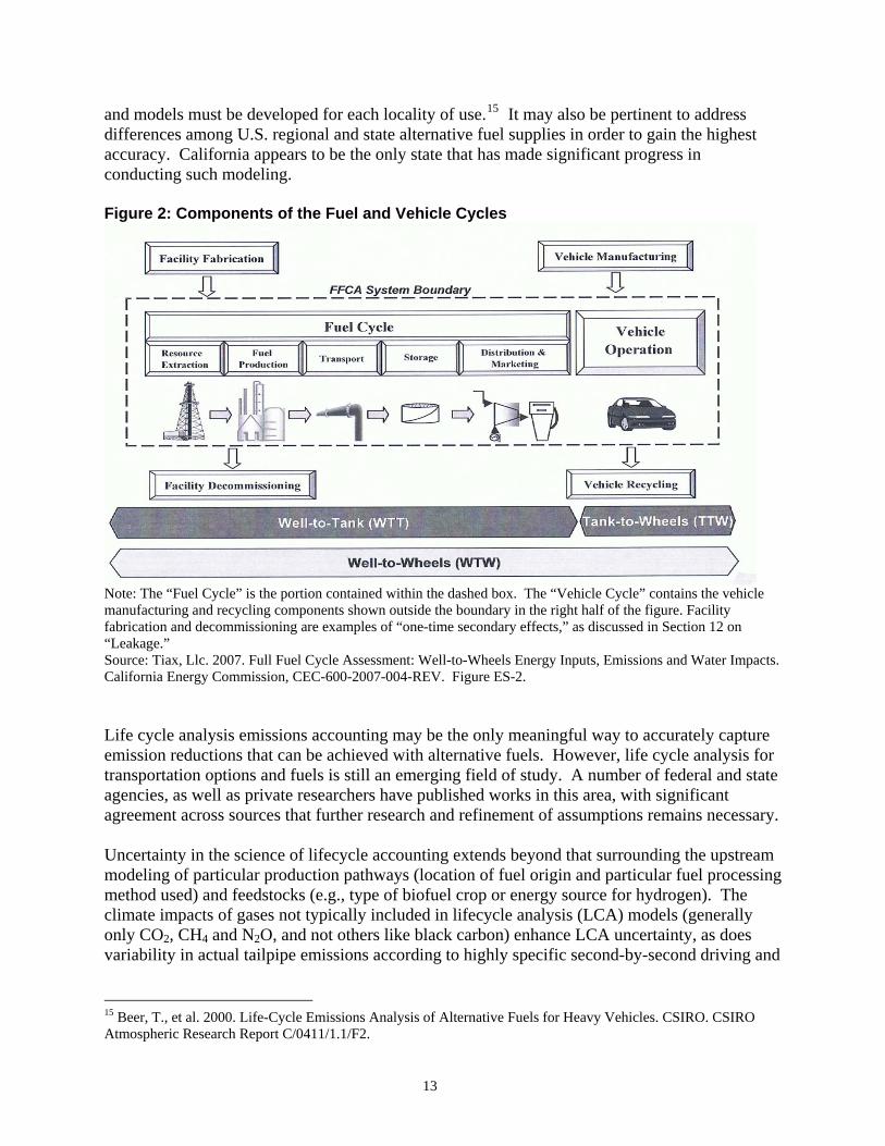
and models must be developed for each locality of use.15 It may also be pertinent to address differences among U.S. regional and state alternative fuel supplies in order to gain the highest accuracy. California appears to be the only state that has made significant progress in conducting such modeling. Figure 2: Components of the Fuel and Vehicle Cycles

Note: The “Fuel Cycle” is the portion contained within the dashed box. The “Vehicle Cycle” contains the vehicle manufacturing and recycling components shown outside the boundary in the right half of the figure. Facility fabrication and decommissioning are examples of “one-time secondary effects,” as discussed in Section 12 on “Leakage.” Source: Tiax, Llc. 2007. Full Fuel Cycle Assessment: Well-to-Wheels Energy Inputs, Emissions and Water Impacts. California Energy Commission, CEC-600-2007-004-REV. Figure ES-2. Life cycle analysis emissions accounting may be the only meaningful way to accurately capture emission reductions that can be achieved with alternative fuels. However, life cycle analysis for transportation options and fuels is still an emerging field of study. A number of federal and state agencies, as well as private researchers have published works in this area, with significant agreement across sources that further research and refinement of assumptions remains necessary. Uncertainty in the science of lifecycle accounting extends beyond that surrounding the upstream modeling of particular production pathways (location of fuel origin and particular fuel processing method used) and feedstocks (e.g., type of biofuel crop or energy source for hydrogen). The climate impacts of gases not typically included in lifecycle analysis (LCA) models (generally only CO2, CH4 and N2O, and not others like black carbon) enhance LCA uncertainty, as does variability in actual tailpipe emissions according to highly specific second-by-second driving and

15 Beer, T., et al. 2000. Life-Cycle Emissions Analysis of Alternative Fuels for Heavy Vehicles. CSIRO. CSIRO Atmospheric Research Report C/0411/1.1/F2.

13

engine conditions.16 EPA is preparing to publish its latest lifecycle analysis, as required by The Energy Independence and Security Act (EISA) of 2007’s Renewable Fuel Standard (RFS) provisions, to also account for indirect emissions. The publication may help address some of the outstanding uncertainties, but the process has been faced with a storm of controversy. Biofuels producers and some academics worry that the incorporation of the current science, which they argue is too embryonic, into a Federal Rule will harm the development of their industry. Environmentalists have countered that the EPA must still issue the rule, regardless of all the uncertainty, as long as it makes its assumptions transparent, recognizes remaining uncertainties, and makes the Rule revisable as science changes.17 Some unique, fuel-based considerations arise when attempting to incorporate upstream emissions. For example, a tailpipe emissions analysis neglects the extraction, production and refining emissions as well as emissions from transportation and distribution. If other fuels are included in an upstream analysis in addition to conventional gasoline and diesel, these emissions should also be accounted for. Other issues, unique to each fuel are discussed below: Biofuels. A switch to biofuels may result in lower tailpipe CO2 emissions if the biogenic, or plant-derived, fuel replaces conventional fossil fuels. This is because the CO2 emitted from combusting biogenic material is assumed to be recycled in the carbon cycle through absorption in the next crop. As a result, by accounting convention, CO2 from the combustion of biofuels in the vehicle or during upstream production and transportation of the fuel is not counted as an emission. Biofuels have faced the greatest scrutiny and uncertainty among alternative fuels. The net GHG benefit of biofuel usage relative to conventional fuels depends heavily upon the feedstock used to create the fuel. This is because of variation in the energy content and conversion energy requirements across the many possible biofuels feedstocks. Current commercially available ethanol and biodiesel utilize the primary energy stores of common food crops – corn and soybeans. Future biofuels production will utilize agricultural and forest byproducts and even algae in order to both increase energy return and decrease the utilization of food resources for transportation fuel. While total production and combustion carbon dioxide emissions can be higher for the use of 100 percent biofuel than for fossil fuel, the non-renewable portion of these emissions is substantially lower than that of conventional fuels. Use of 100 percent biodiesel, on a lifecycle basis, has been found18 to emit 43 percent of the CO2, and 31 percent of the CH4 that would be emitted from a comparable bus that operated on conventional diesel. The direct GHG emissions contribution of various characteristics of agricultural production (fertilizer, tractor fuel, water use, and harvesting) and the use of different resources (fossil and 16 Kammen, D. A. Farrell, R. Plevin, A. Jones, G. Nemet, and M. Delucchi. 2008. Energy and Greenhouse Gas Impacts of Biofuels: A Framework for Analysis. Transportation Sustainability Research Center, U.C. Berkeley. Research Report UCS-ITS-TSRC-RR-2008-1. At: http://repositories.cdlib.org/cgi/viewcontent.cgi?article=1005&context=its/tsrc. 17 Geman, B. “Biofuels companies press EPA, Calif. on lifecycle emissions.” Climate Wire, E&E News. 27 October 2008. 18 Beer, T., et al. 2000. Life-Cycle Emissions Analysis of Alternative Fuels for Heavy Vehicles. CSIRO. CSIRO Atmospheric Research Report C/0411/1.1/F2. Table 3.1.

14

biological) to provide the energy needed to process the fuel can be relatively well calculated and have been the subject of modeling studies for over a decade (see Figure 3). Indirect emissions implications, however, are less well understood and remain a subject of ongoing study.

Figure 3. “Well-to-Wheels” CO2 Emissions from Alternative Fuels19

Sources: Adapted from NRDC: “Getting Biofuels Right”; http://www.nrdc.org/air/transportation/biofuels/right.pdf. Wang et al., 2008. Notes: 1. “Well to Wheels” is another term for “life-cycle.” 2. These estimates include emissions due to U.S. land-use changes estimated to occur at the 4 billion gallon production level. Current U.S. production is already over 6 billion gallons, so the estimates of emissions due to land-use change are already out of date. No emissions due to land-use change are included for Brazilian ethanol because available studies to date indicate that ethanol production does not induce land-use change in Brazil (Fagundes, et. al. 2007). 3. NG = natural gas 4. CCD = carbon capture and disposal. In effect, some of the CO2 removed from the atmosphere during photosynthesis is not returned to the atmosphere but rather is permanently (or for very long time periods) kept out of the atmosphere. Storage of CO2 in geologic formations is one way to do this. 5. The negative emissions shown in the case of ethanol produced from switchgrass with the use of CCD mean that this pathway would remove more CO2 from the atmosphere than is emitted. Sources of uncertainty surrounding indirect emissions from biofuel production center on the conversion of land, particularly forest lands, to biofuel crop lands, which may lead to a net reduction in carbon sinks due to deforestation. The emissions consequences of other indirect (market driven) consequences of biofuels production, such as shifts in international food markets, remain highly uncertain as well.20

19 Peña, N. 2008. Biofuels for Transportation: A Climate Perspective, Pew Center on Global Climate Change, http://www.pewclimate.org/docUploads/BiofuelsFINAL.pdf 20 “No Date Set for EPA Biofuel Emissions Report; Opinion Divided on Land Use Change.” 14 November 2007. 25 x ’25. At: http://www.25x25.org/index.php?option=com_content&task=view&id=665&Itemid=191.

15

The variety of possible fuel ‘pathways’ and the potential direct and indirect effects of each step in the process necessitate additional analyses.21 Limited data due to the relatively recent emergence of the global biofuels market, concerns about data accuracy, and/or uncertainties in the calculations themselves present challenges for the analysis. Even where a particular gallon of ethanol may be traced through a single production plant back to the fields in which the corn was grown, calculating the carbon balance of agricultural production is itself an uncertain science, much less the full integrated process with both its direct and indirect implications on emissions and associated markets.22 The supply of biodiesel in the U.S. is relatively uniform because the present market is fairly homogeneous in feedstock and in production methodology as compared to the future array of possible feedstocks and processing techniques. Current supply includes 60% domestically-grown and similarly processed (using transesterification) soybean-derived biodiesel.23 While the market may be expected to grow in both technological complexity and overall size, all U.S. supplies of both ethanol and biodiesel are subject to tracing requirements stipulated in the RFS which may help to mitigate the impact of industry growth on the complexity of emissions accounting. Under this requirement, the feedstock and producer are tracked via a Renewable Identification Number (RIN). Thus, the primary source of uncertainty for biofuels does, and will increasingly lie in the concept of indirect emissions and the assumptions made about the effects of different biofuel feedstocks on land use and other indirect market effects of production. Lifecycle analyses of biofuels account for fossil- and bio-derived CO2 separately and may include both components or only the non-renewable portion in their emission factors. Only the fossil fraction should be included in the emission factors used in calculating project emissions, the performance standard and the baseline. Accounting for carbon cycling results in an overall GHG reduction compared to non-renewable fuels. Natural Gas. There is still some uncertainty related to the overall tailpipe and lifecycle GHG emission benefits of heavy duty natural gas buses. Some fuel pathways, engine types, and drive cycles lead to lower overall emissions while others increase emissions. Figure 1 above, which illustrates lifecycle model results for buses in California, shows a net benefit from natural gas-based fuels compared with diesel. Other studies comparing vehicle and fuel types show less conclusive results.24 A major source of this uncertainty is in the tailpipe portion of the lifecycle analysis. Table 6 provides a sample of results from dynamometer testing of tank-to-wheel emissions from heavy duty vehicles. 21 For one discussion of the pathways and potential impacts, see Kammen, D., et al. 2008. Energy and Greenhouse Gas Impacts of Biofuels: A Framework for Analysis. Transportation Sustainability Research Center, U.C. Berkeley. Research Report UCS-ITS-TSRC-RR-2008-1. At: http://repositories.cdlib.org/cgi/viewcontent.cgi?article=1005&context=its/tsrc. 22 Turner, B., R. Plevin, M. O’Hare, and A. Farrell. 2007. Creating Markets for Green Biofuels: Measuring and Improving Environmental Performance. Transportation Sustainability Research Center, U.C. Berkeley. Research Report UCS-ITS-TSRC-RR-2007-1. At: http://repositories.cdlib.org/cgi/viewcontent.cgi?article=1000&context=its/tsrc 23 Statistic provided in phone conversation with employee at the Washington, DC office of the National Biodiesel Board, December 2008. 24 Christina Davies, Jette Findsen, and Lindolfo Pedraza, Assessment of the Greenhouse Gas Emission Benefits of Heavy Duty Natural Gas Vehicles in the United States. Final Report, September 22, 2005 http://climate.dot.gov/publications/docs/natgasvehic092205.pdf

16

Table 6. Comparison of Tailpipe CO2 and CH4 Emission Results from Dynamometer Studies of Heavy Duty Vehicles25

Fuel Type Vehicle

Type/Control Technology

Drive Cycle

Mean CH4

Emissions (g/mi)

Mean CO2 Emissions from Same

Sample (g/mi)

GWP- Weighted Emissions

CO2e (g/mi)

LNG Transit Bus Arterial cycle 11.8 1,717 1,988

Transit Bus Triple Length CBD 9.5 2,495 2,714

Buses (1999 DDC Series 50G) CBD cycle 16.4 2,287 2,664

Buses (1999 DDC Series 50G)

NY BUS cycle 54.5 5,609 6,863

CNG

Buses Not specified 12.4 Not reported Not available

Advanced HD vehicles FTP cycle 0.004 1,588 1,588

Moderate HD vehicles FTP cycle 0.004 1,627 1,627

Diesel

Uncontrolled HD vehicles FTP cycle 0.004 1,765 1,765

The primary factor affecting the relative attractiveness and emissions uncertainty of natural gas fuels is the emission of methane, the principal component of natural gas and a relatively potent GHG. Methane emissions arise from incomplete combustion in the engine, as well as from well-to-tank leakage from processing, transportation and fueling infrastructure. As a result, natural gas buses tend to show higher methane emissions (both upstream and at the tailpipe) than conventional diesel buses. Pipeline natural gas is a relatively uniform commodity across the country in terms of quality and energy content. The full emissions profile of CNG and LNG production, however, can vary significantly. This variation results from the range of possible energy sources used for liquefaction or compression, and whether the process takes place on- or off-site relative to vehicle fueling. Methane leakage in processing and transport can also vary widely according to production geography. One Argonne National Laboratory study26 finds that the well-to-tank emissions, per million Btu, associated with CNG differ by 10,000 g CO2e (more than 50%) between North American and non-North American sources. The future use of renewable energy for compression and other upstream process components and expected advances in natural gas engine efficiency will likely yield further net emissions benefits

25 Ibid. 26 Wang, M., and He, D. 2001. Part 1: Well-to-Tank Energy Use and Greenhouse Gas Emissions of Transportation Fuels. Fig. 1.17. At: http://www.fischer-tropsch.org/DOE/DOE_reports/10556/ANL-ES-RP-10556,%2008-23-01.pdf

17

for the use of CNG. However, their future potential constitutes another source of uncertainty in the current fuel cycle models.27 Biomethane-based natural gas fuels may also become commercially viable in the future and will be subject to their own fuel cycle analysis methods and uncertainties. Hybrid Electric. Diesel-electric hybrid buses have become a viable technological and financial option over the past few years such that they now represent a significant portion of new bus orders and manufacturing.28 Similar to conventional diesel buses, most of the emissions from these buses occur at the tailpipe, and most of the emissions consist of CO2 from diesel combustion. In general, the GHG emissions of hybrid electric buses are lower than that of conventional diesel buses, but the full benefits of hybrids depend heavily on the fraction of time the bus operates in electric as opposed to diesel mode. The extent of fuel efficiency improvement realized will vary within a fleet depending on the operational circumstances, primarily the time spent at low speeds, in stop-and-go urban traffic, and idling. Uncertainty surrounding the calculation of emissions benefits is equal to that for diesel fuel, for which tailpipe, upstream processing and transportation pathways are relatively well understood. Fuel Cells. Fuel cell vehicles result in no tailpipe GHG emissions, as they emit just water and hydrogen. Upstream emissions incurred in the generation of the hydrogen fuel can vary significantly depending on the fuel ‘pathway.’ However, hydrogen (H2) pathway emissions are relatively well understood with multiple studies finding similar results. An Argonne National Laboratory study29 of ten common hydrogen pathways, for example, found that all pathways except that using U.S. grid average electricity for electrolysis on average have lower well-to-wheels GHG emissions than do the baseline gasoline vehicles against which emissions were compared. Further, the study found that upstream GHG emissions benefits vary according to the form of the final hydrogen product as either a gaseous or liquid fuel, with liquefaction requiring additional energy and therefore reducing the GHG benefits in all cases except where renewable energy is used. Variability of fuel cell emissions estimates is primarily of concern with respect to the grid-electric electrolysis pathway. The uncertainty range, represented graphically by error bars in the ANL study, indicates that the potential GHG emissions penalty of this fuel pathway relative to gasoline is highly variable, but none the less remains positive. The California Energy Commission,30 in contrast to the ANL study, found a GHG benefit for this pathway, with the difference likely attributable to the relatively clean profile of California electricity resources. Plug-In Electric. The degree to which battery electric vehicles can reduce fuel cycle GHG emissions from fleets is highly dependent on how the ‘fuel’ (electricity) is generated, i.e., is the electricity source a fossil fuel, nuclear, or renewable energy plant? As a result, adequate data on how a fleet’s electricity is produced is significant for the development of a performance standard.

27 Tiax, Llc. 2007. pg.31. 28 Alternative Fuels Data Center, U.S. Department of Energy. 2008. New Buses Built by Fuel Type. Updated 5 November 2008. At: http://www.afdc.energy.gov/afdc/data/vehicles.html 29 Wang, M. 2002. Fuel Choices for Fuel Cell Vehicles: Well-to-Wheels Energy and Emissions Impacts. At: http://www.afdc.energy.gov/afdc/vehicles/emissions_hydrogen.html. 30 Tiax, Llc. 2007.

18

Ideally, if a national standard is used, CO2e emissions data from electricity generation should be obtained by metropolitan area, since this would allow for the most accurate quantification of emissions for electric vehicles (note, this overlaps with issues related to the baseline calculation). In the case that such data is not readily available, the U.S. EPA database eGRID31 could be used, which contains CO2e emissions in lbs per MWh of electricity generated by state, eGRID subregions, NERC regions, and the U.S. overall. If CCAR decides to use fleet-specific performance standards, the best approach would be to obtain information on the generation mix directly from the utility supplying power to the fleet. Once an electron enters the grid it is indistinguishable from those generated by other plants. The practice of applying emission factors for the most specific source definition possible (e.g., single unit where a dedicated generation contract is in place, or eGRID subregion where the provider is unknown) is well established. The available data and relative methodological uniformity make the upstream accounting for plug-in vehicles much more straightforward and accurate than that for a cubic foot of CNG or gallon of diesel.

4. Datasets and GHG Protocols for Transit Fleets 4.1 Datasets on Bus Fleets National Transit Database: There is only one database of national transit statistics that provides detailed information on bus fleets including the number of vehicles in the fleet, miles driven, and fuel consumed by type. This is the National Transit Database (NTD),32 which is published by the Federal Transit Administration (FTA). As a result, the type of performance standard that could be developed for a protocol covering specific vehicle fuel types not included in the EPA protocol (e.g., buses that run on natural gas, fuel cells, electricity only and biofuels) will be directed by the information available in this database. Other organizations, such as the American Public Transportation Association, provide statistics on transit fleets but these sources do not provide activity data for individual fleets. Area-specific Databases: No publicly available regional- or municipal-level databases on transit fleet, mileage and fuel use appear to be available to date. A California transit fleet requirement to report vehicle data annually into a statewide transportation database has been in effect since 2001. Reporting requirements, however, are limited to vehicle, engine and fuel type and does not require the submission of fuel consumption data, nor does it cover any buses in the transit fleet that do not run on some amount of diesel fuel. eGRID: In order to be able to evaluate CO2 emissions for transit buses that run on electricity only, the U.S. EPA Emissions & Generation Resource Integrated Database (eGRID)33 provides data on CO2 emissions in pounds per megawatt-hour of electricity generated by state, eGRID

31 http://www.epa.gov/cleanenergy/energy-resources/egrid/index.html 32 http://www.ntdprogram.gov/ntdprogram/ 33 http://www.epa.gov/cleanenergy/energy-resources/egrid/index.html

19

subregions, North American Electric Reliability Corporation (NERC) regions, and the U.S. overall. While this dataset is readily available and updated every few years to reflect changes in the electricity mix, several characteristics of eGRID have generated uncertainty for emissions accounting. When applied to the charging of plug-in bus batteries, which would more likely be charged overnight while buses are out of service and electricity rates are lower, the inability of eGRID to distinguish between peak load and baseload source emission factors becomes an issue. Even the subregional aggregation of published eGRID factors masks the potentially large differences among local providers’ emissions and the selected eGRID factors may therefore not accurately represent the actual electricity source of the project proposer. Ideally, an emission factor for known and verifiable sources occurring at night should be developed using data on baseload generation in the local power pool. This data could be derived from the underlying eGRID database. Such an approach would increase accuracy, but impose a time burden on the project proposer. 4.2 Other GHG Project Protocols for Transit Fleets Other transit fleet upgrade and fuel switching GHG emission reduction project protocols already exist. However, they do not fully address the breadth of project type possibilities or quantification issues that are of concern to CCAR. Still, there are some components of these methodologies and relevant data resources that may be useful in the development of a transit fleet project protocol. The relevant protocols include: U.S. Environmental Protection Agency (EPA), Climate Leaders: Transit Bus Efficiency (August 2008).34 Potential GHG offset projects could include: early retirement of existing buses and replacement with more efficient buses; conversion of existing buses to cleaner fuel/engine systems; switching to a more efficient fuel/engine system when replacing buses at the end of their service life; and adoption of more efficient fuel/engine systems when expanding the transit fleet to meet increased service demand. Only those buses fueled by gasoline, diesel, or oil-based propane are eligible to use the EPA offsets protocol. The protocol is based on a performance standard for tailpipe emissions only, and is expressed in terms of grams of CO2 per miles driven. It provides two separate thresholds: one for small cities and another for large cities. Clean Development Mechanism (CDM): AMS-III.S.: Introduction of low-emission vehicles to commercial vehicle fleets (Valid from Nov 30, 2007 onwards).35 This methodology is for project activities introducing low-GHG emitting vehicles for commercial passenger and freight transport, operating on a number of identified fixed routes. The types of low emission vehicles to be introduced include, but are not limited to: compressed natural gas (CNG) vehicles, electric 34 http://www.epa.gov/stateply/documents/resources/transit_protocol.pdf 35 http://cdm.unfccc.int/UserManagement/FileStorage/CDM_AMSF01BV5SB5QCEMPNM5K5QV 1C5B2TUL4

20

vehicles, liquefied petroleum gas (LPG) vehicles, and hybrid vehicles with electrical and internal combustion motive systems. The types of vehicles covered by the methodology include: buses (public transport), and trucks (freight transport). The methodology only includes tailpipe CO2 emissions in the project boundary and, where applicable, the upstream CO2 emissions from electricity generation for plug-in electric vehicle projects. Emissions associated with the upstream processing of natural gas fuels, which includes both fugitive CH4 and process-related CO2, are considered ‘leakage’ under this methodology and are not accounted for unless the project is part of a “Programme of Activities.”36 In such cases, CH4 is accounted for separately using the leakage methodology developed as part of the consolidated methodology for fuel switching from coal or petroleum fuel to natural gas (ACM0009). Nitrous oxide emissions are not calculated for any portion of the fuel cycle. Methane emissions from the tailpipe are not calculated either, even in the case of projects involving a switch to natural gas-based fuels.

5. Performance Standard Development A performance standard sets a threshold emissions level that is significantly better than the average emissions performance for a specified service. It can also be used for establishing the baseline for projects to meet new demand or to replace vehicles at the end of their service life. In this case, we expect the threshold to be set by reference to the emissions performance of transit fleets. If a project for improving fleet performance has emissions that are equal to or better than the threshold, then the project would be considered to exceed the “business-as-usual” (BAU) performance and would be eligible for registration of emission reduction credits. In this section, we highlight specific issues that need to be considered when developing a threshold for transit bus fleet projects that increase emissions performance by converting transit fleets to run on alternative fuels or by upgrading to hybrid or electric technologies. For comparison, we utilize the only standardized protocol on related projects currently available in the U.S., the EPA Climate Leaders Protocol for “Transit Bus Efficiency.” EPA’s performance standard focuses on CO2 tailpipe emissions from transit buses. Because of the focus on CO2 emissions, only those buses fueled by gasoline, diesel, or oil-based propane are eligible to use this standard. This would include diesel and gasoline hybrid buses.

36 Under the CDM a “Programme of Activities” [PoA] is defined as a “voluntary coordinated action by a private or public entity which coordinates and implements any policy/measure or stated goal (i.e., incentive schemes and voluntary programmes), which leads to anthropogenic GHG emission reductions or net anthropogenic greenhouse gas removals by sinks that are additional to any that would occur in the absence of the PoA, via an unlimited number of CPAs [CDM Programme Activities].” Under the CDM fleet methodology, a PoA could include a national policy that all diesel fleets switch to use of an alternative fuel. Where a project is part of a PoA, emissions calculations for each project must be revised to account for leakage.

21

To allow for a comparison across bus fuel types, EPA used a fuel neutral metric of CO2 emissions per miles driven for the performance threshold. This metric was developed using data from the NTD (described in Section 4.1) and involved the following steps:

• Manually linking data for each transit agency in NTD, annual vehicle miles traveled for all directly operated37 buses, and annual fuel consumption by all directly operated agency buses;

• Multiply fuel consumption by a fuel type-specific CO2 emissions factor; • Sum CO2 emissions across fuel types used by bus mode for each transit agency; • Divide total annual CO2 emissions from buses for each agency by total annual bus

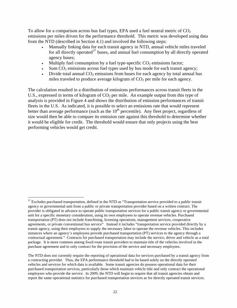
miles traveled to produce average kilogram of CO2 per mile for each agency. The calculation resulted in a distribution of emissions performances across transit fleets in the U.S., expressed in terms of kilogram of CO2 per mile. An example output from this type of analysis is provided in Figure 4 and shows the distribution of emission performances of transit fleets in the U.S. As indicated, it is possible to select an emissions rate that would represent better than average performance (such as the 10th percentile). Any fleet project, regardless of size would then be able to compare its emission rate against this threshold to determine whether it would be eligible for credit. The threshold would ensure that only projects using the best performing vehicles would get credit.

37 Excludes purchased transportation, defined in the NTD as “Transportation service provided to a public transit agency or governmental unit from a public or private transportation provider based on a written contract. The provider is obligated in advance to operate public transportation services for a public transit agency or governmental unit for a specific monetary consideration, using its own employees to operate revenue vehicles. Purchased transportation (PT) does not include franchising, licensing operations, management services, cooperative agreements, or private conventional bus service” Instead it includes “transportation service provided directly by a transit agency, using their employees to supply the necessary labor to operate the revenue vehicles. This includes instances where an agency’s employees provide purchased transportation (PT) services to the agency through a contractual agreement.” Contracts for purchased transportation may include the service, driver and vehicle as a total package. It is more common among fixed route transit providers to maintain title of the vehicles involved in the purchase agreement and to only contract for the provision of the service and necessary employees. The NTD does not currently require the reporting of operational data for services purchased by a transit agency from a contracting provider. Thus, the EPA performance threshold had to be based solely on the directly operated vehicles and services for which data is available. Some transit agencies do possess operational data for their purchased transportation services, particularly those which maintain vehicle title and only contract the operational employees who provide the service. In 2009, the NTD will begin to require that all transit agencies obtain and report the same operational statistics for purchased transportation services as for directly operated transit services.

22

Figure 4. CO2 Emissions Performance of US Transit Bus Fleets Using EPA Offsets Approach

Cumulative Percent of Transit Buses that Meet or Exceed Emissions Level

0%10%20%30%40%50%60%70%80%90%

100%

0.0 1.0 2.0 3.0 4.0

CO2 Emissions Performance (kg CO2 per Mile)

Cum

ulat

ive

% o

f Fle

et's

Bus

es

that

Mee

t or

Exce

ed

CO

2 Em

issi

ons

Leve

l

Top 10th percentile (2.058 kg/mi)

Top 25th percentile (2.390 kg/mi)

Weighted average (2.765 kg/mi)

Best bus in data set (1.453 kg/mi)

As will be discussed further below, there are significant spatial issues that affect the drive cycle and thus emissions performance of transit fleets. EPA accommodated some of these in their methodology. Referencing the different driving conditions (e.g., stop-and-go traffic) in larger metropolitan areas versus smaller metropolitan areas, EPA developed separate thresholds for cities with a population of more than one million (referred to as “large metropolitan areas”) and less than one million (referred to as “small metropolitan areas”).38 However, the methodology may still exclude some outlier fleets with extremely high stop-and-go traffic, such as that in New York City, because those buses would be much less efficient than average fleets in the U.S. The following subsections explore other approaches than the one used by EPA to determine whether there is a better way to reflect geographic differences among fleets and whether it is possible to expand the performance standard beyond oil-based buses to also include natural gas, electric, biofuel, fuel cell, and hydrogen buses. It also examines whether it would be possible to develop performance thresholds for other types of fleets, such as commercial long-haul or school buses. One alternative option we consider is whether the threshold should be set based on individual fleet emission rates, rather than a national emission rate. In this case, the framework for

38 The performance threshold for both large and small metropolitan areas, areas with greater than or less than one million people, respectively, was set at the top 10th percentile of the CO2 per miles driven of the typical transit bus emission rate in each of the areas. For large metropolitan areas, proposed projects have to meet or exceed 2.11 kg CO2 per mile; for small areas, they have to meet or exceed 1.46 kg CO2 per mile.

23

establishing the emissions threshold would be similar to that outlined for EPA above, except instead of selecting the threshold emissions rate from the whole range of bus fleets in the U.S. (as illustrated in Figure 4), the threshold would be selected from the range of emission performances of all the vehicles within an individual fleet. If CCAR selected the 10th percentile as the cut-off for transit fleet projects, proposed projects would then have to perform better than or equal to the 10% best performing vehicles within their own fleet. As will be outlined below some of the considerations in going beyond EPA’s approach include:

- Spatial variations in fleet operations which make the use of a national level threshold less representative of performance by all fleets;

- Limited availability of data on fleet characteristics; - Challenges in creating a metric for emissions performance that enables comparison

across all types of fuels; and - Lack of established emission factors for estimating upstream emissions from alternative

fuels. 5.1 Spatial Categorization The EPA protocol uses performance standards, based on national data, for large and small metropolitan areas. This spatial categorization was developed because transit agencies in large urbanized areas typically experience similar patterns of stop-and-go, short acceleration and deceleration cycles associated with heavy vehicular traffic. These patterns differ from those in cities with smaller populations where traffic is often less dense and bus stops may be more widely spaced, resulting in more continuous driving conditions and therefore likely lower vehicle emissions. As noted in the EPA protocol, these performance thresholds may not be applicable for all transit bus types and operating circumstances. Factors, such as drive cycle, significantly impact the emissions performance of individual vehicles. Certain alternative fuel and engine types are better suited to particular drive cycle demands than are others. CNG buses for example, which typically have spark ignition engines, will experience a greater fuel economy penalty relative to diesel for routes with short cycles of frequent stop-and-go operation. This is due to the lower thermal efficiency of spark ignition engines compared to diesel compression engines when operated at low speed.39 As a result, there may be cases where select vehicle types cannot exceed a national performance standard, but may instead be able to pass a threshold based solely on fleet operations under similar driving conditions. In addition, average temperatures and weather conditions affect the efficiency of a given fleet. Cold climates reduce conventional engine combustion, whereas extremely warm climates limit the amount of regenerative braking energy that can be absorbed by the battery packs in electric and hybrid vehicles. Additionally, relative to diesel or alternative fuel vehicles, hybrids experience a higher percentage fuel economy penalty in the summer due to the operation of air conditioning systems. An on-road year-long test of ten hybrid buses operated by NYC Transit 39 Barnitt, R. and K. Chandler. 2006. New York City Transit (NYCT) Hybrid (125 Order) and CNG Transit Buses: Final Evaluation Results. NREL Technical Report: TP-540-40125. At: http://www.nrel.gov/vehiclesandfuels/fleettest/pdfs/40125.pdf

24

found that the average monthly diesel fuel economy improvement of the hybrids compared with conventional vehicles dipped as low as 12% in June and was highest (up to 52% improvement) in February and March.40 Winter diesel fuel blends can also have lower energy content, and correspondingly lower fuel economy,41 affecting the per mile emissions performance of conventional, biodiesel blend and hybrid diesel-electric vehicles operating in cold climates. Another geographic issue that affects a given fleet’s efficiency is the topography the vehicles experience during operation, e.g., the steep hills of the San Francisco Bay Area versus the relatively flat landscape of New York City. Such “grade effects” dictate engine power requirements at a given speed and will alter fuel economy and emissions performance of different engine types in different ways.42 It may also penalize AFV projects located in more hilly terrains if the efficiency penalty is so great that they cannot meet a threshold based on a national average topographic profile. Vehicle passenger load can also vary significantly across routes and agencies, affecting overall vehicle weight, which is another determinant of fuel economy.43 Fleets that, on average, operate buses that tend to either be near-empty or standing room only present a source of operating variability not captured by the simple delineation of small and large urban areas in the EPA methodology. A detailed categorization and analysis of U.S. transit fleet data according to the spatial and geographic considerations would be necessary in order to quantify the impacts of the geographic, grade and load effects outlined above. For geographic and grade effects, such an analysis could be accomplished by using the fleet activity data provided in the NTD and would entail manually importing and grouping fleets according to heating and cooling degree days for each city or suburban area and the altitude differential across each agency’s service territory. Since passenger load is not necessarily a function of any other population or spatial characteristic, a separate analysis according to agency average passenger ridership per vehicle could be undertaken via the calculation of passenger miles per vehicle revenue mile. Such an analysis could help determine if the use of a fleet-specific performance standard that accounts for both vehicle type and load would be necessary to control for the influence of this factor. However, this type of analysis is not possible using NTD data, because the average occupancy percentage per bus type is not reported to this database. Passenger trips and passenger miles are reported per fleet only. The only way to obtain the requisite data would be to survey a sample of fleets in the U.S. Variations in fuel economy are relevant to all bus types, but are particularly important in the analysis of hybrid diesel-electric vehicles. A number of studies using laboratory-based dynamometer emissions testing have looked at the impact of different drive cycles on emission 40 Barnitt, R. and K. Chandler. 2006. 41 http://www.pacific-biofuels.com/staenergy.asp?id=res&subid=staenergy 42 Clark, N., F. Zhen, W.S. Wayne, and D. Lyons. 2005. Transit Bus Life Cycle Cost and Year 2007 Emissions Estimation. Federal Transit Administration Final Report FTA-SV-26-7004.2007.1 At: http://www.fta.dot.gov/documents/WVU_FTA_LCC_Final_Report_07-23-2007.pdf 43 Kilma Climate Change Center. 2005. “Engine Design Improvements.” At: http://www.klima.ph/cth/solutions/engine_design/engine_design_improvements.php

25

rates. The range of rates found in these tests is so great that some fleets may not be able to meet a national-level performance standard. For example, a study conducted by the National Renewable Energy Laboratory for King County Metro in Washington State found that the fuel economy improvement for diesel-electric hybrids compared with conventional diesel was 30% under conditions representative of the King County drive cycle (and 26% in actual usage). The improvement was 75% for test runs using a drive cycle characteristic of a Manhattan bus.44 Lab-based tests, however, are unable to account for the terrain and weather characteristics that also affect vehicle emissions performance. On-road test comparisons of operation in varying terrain conditions do not appear to be available. One chassis-dynamometer study of diesel bus emissions suggests that “grade effects” may be calculated using an equation for theoretical power requirement.45 The next generation of emissions models, known as “load-based modal” models, are beginning to include such calculations. For example, U.S. EPA’s MOVES model will first calculate engine power requirements based on operating conditions (e.g., load, terrain) and then calculate emissions.46 Another spatial issue to consider is whether additional levels of geographic aggregation will be needed to reflect differences in the sourcing of the replacement fuels. In addition to regional differences in grid-based electricity supply, the upstream emissions associated with any particular conventional or alternative fuel may vary from city to city, but the variability in pathways and upstream efficiencies is currently much greater for alternatives. Locally-produced soybean-derived biodiesel in a Midwestern state has lower transportation-related upstream emissions than imported Brazilian soy biodiesel. It is also less likely to have been grown on land that was recently converted from high carbon value forest to relatively low carbon agricultural production, and thus would have lower indirect emissions. Similarly, compressed natural gas produced in high-efficiency domestic operations will have lower upstream methane emissions associated with leakage during processing and transport. In light of these issues, a fleet-specific performance standard may be a better approach. Fleet operators would then use a standard calculation framework specified by CCAR in conjunction with their own activity data reflecting the particular bus engines, miles driven, and fuels consumed by their current fleet. Such an approach would likely increase the number of fleets covered by the protocol, but would also make the performance standards less uniform across the U.S.

44 Chandler, K. and K. Walkowicz. 2006. King County Metro Transit Hybrid Articulated Buses: Final Evaluation Results. NREL Technical Report TP-540-40585. 45 Kern, J. 2000. Inventory and Prediction of Heavy Duty Diesel Vehicle Emissions. West Virginia University. At: https://eidr.wvu.edu/files/1245/kern_j_etd.pdf. 46 http://www.epa.gov/nrmrl/pubs/600r07106/600r07106.htm, and http://etd.gatech.edu/theses/available/etd-04052007-194445/unrestricted/feng_chunxia_200705_phd.pdf

26

5.2 Eligibility of All Bus Fuel Types There are three major considerations involved with setting a performance standard that includes all fuel types such as diesel, natural gas, fuel cells, electricity, biofuels, and hydrogen. This includes:

- Availability of established emission factors for characterizing upstream emissions; - The existence of a common metric for comparing emissions across different fuel types,

regardless of tailpipe and upstream differences; and - Availability of data on fuel consumed and miles driven by individual vehicles within the

fleets. Emission Factors for Characterizing Upstream Emissions As outlined in Section 3, all non-petroleum based fuels lead to significant upstream emissions of CO2, CH4, and N2O. In the case of electricity and hydrogen buses, all emissions would be upstream. A performance standard must therefore be able to accurately reflect these upstream emissions in the threshold rate. However, except for electricity, there are not yet established upstream emission factors for most of these fuel types. Instead, a range of emission factors and pathways have been used to analyze different heavy duty vehicle categories in different regions. In some cases, the uncertainties may be too great to resolve completely. For example, so far, it has not been possible to fully quantify the potential for upstream source and processing leakage from natural gas production. One study ties differences between North American and non-North American-sourced natural gas to differences in production efficiency and standards for transportation and storage. The study finds than non-North American CNG can use nearly twice the fossil energy and produce nearly twice the upstream GHGs as compared to North American production.47 The problem of variable upstream leakage can be mitigated in cases where the natural gas source and pathway are known and the emission factor for the closest, or most likely, pathway can be selected and applied. However, this would be difficult when developing standardized emission factors for a performance threshold, unless the offsets program leaves it up to the fleet operator to determine the upstream emission factors for its natural gas. However, fleet operators may not always know the source of their fuel either. Overall, natural gas buses pose the greatest challenge because, as outlined in Section 3, when both tailpipe and upstream emissions are factored in, it is not always clear that these buses reduce GHG emissions when compared to similar buses using conventional fuels. In the case of U.S. biofuels, the fuel sources are still relative few and the accounting standards for these are fairly known. As a result, it would be possible to ask fleet operators to calculate upstream emissions associated with these fuels, but it would be difficult to develop a national estimate because there is no national dataset linking biofuel use and source to individual fleets. 47 Wang, M., and He, D. 2001. Part 1: Well-to-Tank Energy Use and Greenhouse Gas Emissions of Transportation Fuels. Figs. ES-1.2, ES-1.4. At: http://www.fischer-tropsch.org/DOE/DOE_reports/10556/ANL-ES-RP-10556,%2008-23-01.pdf

27

In the future, as the biofuels market diversifies, it may become hard even for fleet operators to determine the source and emissions profile of their biofuel. To overcome these issues, CCAR could do the following:

- Undertake its own study to review and select emission factors for each fuel type. For example, Beer, et al.,48 explore the fuel production CO2, CH4 and N2O emissions for geographically specific supplies conventional and alternative fuels. Such studies may provide the basis for the development of an “acceptable” range of upstream emissions for each particular fuel type that could be coupled with either an engine and control technology specification (see technology-based standard below) or tailpipe emissions metric for each given fuel type. However, this may be time consuming and may not resolve all uncertainties. Some level of uncertainty surrounding tailpipe and upstream emissions of must be accepted if the protocol is to extend over the range of possible vehicle fuels.

- Exclude some of the more uncertain fuels from the performance standard, such as natural gas, fuel cells, and hydrogen, until more conclusive emission factors have been developed.

- Adopt a fleet-specific performance standard framework since fleet operators most likely would have sufficient information on the source and consumption of biofuels.

Performance Metrics Setting a performance standard encompasses two key issues, the stringency of the value itself and the units to express the value in. In the EPA protocol, the performance standards focus specifically on CO2 tailpipe emissions from transit buses, which is sufficient because the methodology only covers buses fueled by gasoline, diesel or oil-based propane. Projects under this protocol have to meet or exceed the top 10th percentile of the amount of CO2 generated per mile driven. While the top 10th percentile threshold may turn out to be a reasonable cutoff for a potential CCAR protocol, the reporting metric (CO2/miles driven) must be reassessed if CCAR decides to expand its methodology to include non conventionally-fueled buses. The EPA approach of assessing only CO2 tailpipe emissions does not accurately represent the entire range of GHG emissions from transit buses running on alternative fuels (e.g., natural gas which has a much higher CH4 content than carbon-dominated traditional fuels) or upstream emissions from vehicles that utilize biofuels, fuel cells, or electricity only which have zero or net zero tailpipe emissions. Due to these considerations, CCAR may wish to consider other metrics and threshold categorizations. The advantages and disadvantages of a number of other possible options are discussed below and summarized in Table 7. These include expressing the standard in terms of CO2 equivalent, energy content, and/or emissions on a ‘per mile,’ ‘per diesel equivalent gallon,’ or ‘per passenger’ unit basis.

48 Beer, T., et al. 2000. Part 2: Fuels.

28

To capture the emissions quantification uncertainties associated with certain fuels and technologies, we also explore developing a standard that ‘weights’ an emissions reduction calculation by the relative uncertainty of the underlying data, i.e., a fuel with less quantification uncertainty could be multiplied by a larger ‘accuracy factor’ in the standard calculation formula than those with higher uncertainty. CO2 per mile: The metric of CO2 emissions per miles driven is the only metric that captures all the factors that determine emissions performance of transit buses in terms of miles driven (i.e., service provided), including fuel efficiency, engine efficiency, and carbon content of the fuel. It also enables the development of a range of emissions performances representing miles driven of transit buses from which a threshold can be selected. To illustrate:

1) Diesel has a much higher energy density (energy per gallon) than alternative fuels (LNG, CNG, and Propane) and therefore is much more efficient when combusted than its alternatives.

2) Diesel engines also operate at a higher thermal efficiency than dedicated alternative fuel engines, which may translate into a fuel economy improvement of up to 25 percent per Btu of diesel fuel used.

3) Meanwhile diesel fuel contains more carbon per unit fuel (i.e., produces more CO2 when combusted) than alternative fuels

Only a “per mile” metric can capture these differences effectively. The CO2 per mile metric only enables comparison across fuels where carbon is the major component of the fuel – i.e., petroleum-based fuels. It does not accurately capture tailpipe emissions from natural gas-based fuels, which have higher methane content, or from fuels with significant upstream emissions. CO2 per Btu Metric: A comparison of CO2 per unit energy (e.g., Btu, MJ, or diesel equivalent gallons) can capture the emissions differences resulting from fuel switching, but does not incorporate changes to fuel use achieved through vehicle efficiency and emissions control applications. In the case of vehicle replacement with hybrid diesel-electric buses, a CO2e per unit energy cannot capture the fuel-saving, and thus emissions-reducing, benefit of hybrid drive engines. The thermal efficiency of some alternative fuel engines can also be significantly inferior to that of diesel, resulting in as much as a 25% reduction in fuel economy per Btu.49 This difference would not be captured by this metric either. Finally, a per gallon or gallon equivalent metric also does not allow assessment based upon the service or output provided from fuel use – the miles driven by each bus. Even if the metric were expanded to include CO2e per unit energy, the metric would still not be able to capture differences due to efficiency improvements. The only type of offset project this metric would capture would be projects that lead to fuel switching towards low carbon content fuels (i.e., a switch from diesel buses to LNG, CNG or 49 Tiax, Llc. 2003. Transit Bus Niche Market for Alternative Fuels: Module 2: Basics of Alternative Fuels in Transit Bus Applications. Clean Cities Coordinator Toolkit. At: http://www.p2pays.org/ref/36/35617.pdf.

29

propane) because diesel would then make up a smaller share of the fuel metric and thus CO2 emissions per gallon of fuel equivalent would be lower. CO2 per Passenger or Passenger Mile Metric: While some transit agencies may wish to report their operating statistics in terms of passengers, it is not a meaningful denominator when comparing lifecycle emissions for vehicle use. Passenger load is a variable factor contributing to vehicle weight which then affects vehicle fuel economy. However, the number of passengers does not provide a comparable metric of ‘service provided’ because passenger load does not necessarily correlate with vehicle emissions or miles driven due to the provision of bus service. An empty bus, for example, will still operate along its scheduled route and emit GHGs regardless of having no passengers. CO2equivalent per Mile Metric: A summation of the upstream and tailpipe GHGs that result from driving one mile would be the best option for capturing the total emissions performance of all types of vehicle fuels. However, this would require:

1) Emission factors for all three GHGs emitted at the tailpipe, including information on miles driven by all natural gas buses in order to estimate CH4 emissions. However, existing CH4 and N2O tailpipe emission factors are highly uncertain.

2) Emission factors for upstream emissions of all three GHG’s for each fuel type. If there are variations within each fuel, it would be necessary to obtain information on the amount of fuel used within these variations.

There are no national datasets that can provide this information. For tailpipe emissions, the NTD does not track miles driven by individual vehicle fuel types. Thus, there is not enough information to apply the emission factors for CH4 and N2O, which are expressed in terms of CH4 or N2O per mile driven for each vehicle technology (see Section 3). Individual fleets do track this information, however, and would be able to estimate emissions at the fleet level. The NTD also does not support the estimation of upstream emissions. It only tracks overall fuel consumption of each individual fleet, and doesn’t provide information on where the vehicle fuels are sourced from. Individual fleet operators would likely know the source of some of their fuels such as biofuels and electricity. However, it would be harder for them to track down information on natural gas and other alternative fuels. Uncertainty Weighted Standards: Regardless of the metric chosen (per mile, passenger or gallon equivalent consumed), CCAR may wish to explore a system by which individual project emission estimates could be weighted (in effect, discounted) according to the level of uncertainty underlying the emission factors applied. Estimates of tailpipe CO2 emissions, for example, have a higher degree of certainty than do those for CH4. This is because CO2 is more directly a result of fuel carbon content, as opposed to technology, engine condition and drive cycle dependent, as is CH4. The same may be said of the application of diesel production emission factors as opposed to those developed for biofuels production. The U.S. diesel market is much more unified in terms of source and efficiency, whereas biofuels may come from a number of feedstocks and

30

production methods. A study by Beer, et al.50 provides a good discussion and data on the statistical emissions variability with respect to both tailpipe emissions and fuel cycle (upstream) emissions (see Chapter 2 of the Beer report). Technology-Based Standard: Another option for developing a standard that allows comparison across all fuel types would be to develop a technology-based standard whereby one would specify the actual engine technology and fuel type (including production pathway) that would represent better than average performance. However, this approach is likely to be equally difficult because it would require extensive datasets on technology and fuel options for fleets, which may be comparable in more general terms but not with the level of specificity necessary to set a meaningful technology (and fuel use) prescription. Additionally, the technology landscape changes over time, necessitating constant revision of the standard. This is particularly relevant with respect to hybrid, battery electric and fuel cell vehicles and the production pathways and market impacts of biodiesel and ethanol worldwide. Table 7: Comparison of Potential Threshold Metrics Standard Type Data Requirements Limitations and Issues EPA Style (CO2/mile) Fuel consumption, miles

driven (fleet wide), service territory, population

Does not incorporate CH4 and N2O from the tailpipe, nor upstream emissions. Thus, excludes non-petroleum based fuels.

CO2e per Gallon Fuel production and combustion emissions

Does not account for cross-fuel differences in energy density, engine thermal efficiency, emissions control application or the level of service provided

CO2e per Btu Fuel production and combustion emissions, energy content relative to diesel

Does not account for cross-fuel differences engine thermal efficiency, emissions control application or the level of service provided

CO2e per Passenger Fuel production and consumption, number of passengers served

Variation in the number of passengers served does not directly link with the resulting emissions from service of miles driven

CO2e per Mile Tailpipe and upstream emission factors, fuel consumption by each fuel (including by each fuel source), and miles driven by each vehicle fuel type

Necessary if comparing across fuels and lifecycles. Requires data characteristics and fine aggregation not available in the NTD.

Uncertainty Weighted Not a metric itself, but an approach to discount project emission reduction calculations where highly uncertain values are applied in estimation.

Technology Specific Dataset on common and better-than-average vehicle technologies

Relatively rapid technological change necessitates frequent revision and in-depth knowledge of technologies and fuel production processes. Does not necessarily reduce uncertainty.

50 Beer, T., et al. 2000. Life-Cycle Emissions Analysis of Alternative Fuels for Heavy Vehicles: Stage 1. CSIRO. CSIRO Atmospheric Research Report C/0411/1.1/F2.

31

5.3 Expanding the Performance Standard to Include Other Bus Fleets In order to expand the performance standard, it is necessary to consider what types of fleets are amenable to standardized offset methodologies. Transit bus fleets51 are clear candidates because, in general, they drive on similar, well-documented routes. Other public or private bufleets, such as those operated by school districts and intercity bus lines also operate hundrethousands of buses across the country and represent another opportunity segment for emissions reductions projects (See Section 2). This is because their routes are similarly standardized, the bus sizes are uniform, and there is not so much variation in the fuels used.

s ds of

While the discussion thus far has centered upon transit fleets, this is primarily due to the public availability of data for use in developing national or regional performance standards and the current transit offset protocol landscape. As mentioned in Section 2, there are no national databases available for school buses and intercity fleets similar to the NTD for transit fleets. As a result, a national-level performance standard for those buses cannot be developed. The only way to include school buses and intercity fleets in an offsets program would be to use a fleet specific framework, whereby CCAR outlines the methodology for data collection and threshold setting and provides standardized emission factors for calculating emissions and reductions. The project proposer would then gather the necessary data to develop a fleet specific threshold. 5.4 Summary and Implications

Expanding the performance standard to include all possible vehicle fuel types would entail the inclusion of tailpipe and upstream GHG emission factors in the calculation of the performance threshold. Because of the limited national-level data on fleet activities, this shift would mean that the performance standard should be fleet-specific since this is the only way that the required activity data can be collected. It would also require additional research by CCAR to select/establish upstream emission factors for all fuels, unless the Registry chooses to exclude fuels with the highest uncertainty such as natural gas, hydrogen, and fuel cells. The advantage of a fleet-specific standard would be the ability of the metric to capture all of the spatial, fleet make-up, operational and maintenance conditions specific to a particular fleet that complicate the application of a single national standard. The development of a fleet-specific performance standard would rely upon data for just the specific fleet(s) as opposed to any public database. Following this approach it would be easier to track down the consumption of various types of fuels to estimate upstream emissions and tailpipe emissions of CH4 and N2O. Another major benefit of using a fleet-specific approach would be that is could very likely be expanded to include other uniform bus fleets, such as school buses and intercity buses.

51 According to the APTA, a transit system is defined as “An organization (public or private) providing local or regional multi-occupancy-vehicle passenger service. Organizations that provide service under contract to another agency are generally not counted as separate systems.” The transit bus category entails “A bus with front and center doors, normally with a rear-mounted engine, low-back seating, and without luggage compartments or restroom facilities for use in frequent-stop service.”

32

Using a fleet specific approach, the time and reporting burden would shift away from CCAR to the fleet operators. This would conflict with one of the goals of the standardized offsets approach which is to relieve the upfront costs to the project developer of preparing offsets projects.

Some metropolitan areas such as NYC have already purchased relatively high numbers of hybrid buses and other alternative fuel vehicles through voluntary programs, but not through regulations. Should these programs be held to the same performance standard requirements as other fleets with relatively few alternative fuel vehicles? Where a transit agency has previously chosen to operate hybrid or alternative fuel buses independent of any regulatory requirement, for reasons such as cost reduction or environmental responsibility, they may be hard pressed to implement even better fleet vehicles if a fleet-based standard were adopted. Or, it is possible that at fleet specific-performance standard would provide even more incentives for improving the emissions performance of fleets, thus increasing the rate at which cleaner vehicles are developed and adopted.

6. Additionality 6.1 Regulatory Additionality The regulatory test involves screening out projects that are already required by other state and federal regulations, as these projects would be part of the business-as-usual scenario. The following discusses regulatory requirements that may affect fleet upgrade projects 6.1.1 Federal Requirements The Energy Policy Act of 1992 (EPACT 1992), Section 303, and Executive Order 13149 establish requirements for federal fleet operators to purchase alternative fuel vehicles. There are no purchasing requirements for heavy duty vehicles and buses. Moreover, even though transit agencies receive heavy government subsidies, they are normally privately owned and, therefore, not covered by such purchasing requirements. Although EPACT 1992 creates vehicle and refueling tax deductions, and encourages voluntary market development, transit bus agencies do not have any mandatory compliance requirements under EPACT or Executive Order 13149. The Energy Policy Act of 2005 does not introduce new requirements pertaining to heavy duty vehicles.52

52 The Corporate Average Fuel Economy (CAFE) standard establishes fuel economy standards for original automobile manufacturers producing light duty vehicles and small trucks. Fuel economy requirements do not apply to heavy duty vehicles, such as transit buses. The U.S. EPA promotes alternative fuel use, and establishes air pollutant emission standards for heavy duty highway engines, including buses, but the regulations do not address GHG emissions or mandate alternative fuels or fuel-efficient vehicles.

33

6.1.2 State and Local Requirements Some states and local governments may encourage the purchase of alternative fueled buses or fuel efficient buses and may have in place voluntary retrofit or early retirement programs for heavy duty vehicles. Below is a discussion of such programs. Low Carbon Fuel Standard: The potential introduction of state-based low carbon fuel standards (LCFS), such as the one being developed in California (CA), will pose specific issues for passing the regulatory test. The LCFS suggests that a state-based threshold would be needed or, at minimum, a single rule for the nation that does not include CA and a separate standard for CA. If other states adopt a similar standard, a timeframe for updating the ‘national’ standard and rules concerning when the update takes effect may need to be devised. The standard also presents a technical consideration, namely that each fuel’s GHG profile (e.g., life cycle emissions) needs to be known to determine compliance with the standard. Since life cycle emissions will vary by region and fuel distributor, this information would then have to be available at the local or regional level in order for the project developer to determine whether they can exceed the performance standard. Furthermore, based on the outcome of CA’s efforts, a procedure might need to be devised for evaluating reductions associated with fuels that have higher uncertainties in their GHG profile values than others. Purchasing Requirements and Criteria Air Pollutant Regulations: New York City’s MTA and NYC Transit were required by the state government in 2000, in exchange for funding from a state bond program, to revise their 5-year purchasing plan to fit all buses with pollution traps, use only ULSD, and to include 300 CNG and 250 hybrid electric vehicles in their new bus orders53. The state of California adopted a Fleet Rule for Transit Agencies54 in 2000 and updated its requirements in 2005. Under this regulation, covered transit agencies are required to reduce their fleet’s diesel-based emissions of NOx and PM. As one alternative compliance path for buses, the rule stipulates that 85% of new bus purchases by 2009 must be alternative fueled. In certain localities, the local air management district has required compliance via the alternative fuel path. Another such example is the King Country Metro Transit agency of King County Washington. In 2006, Washington voters approved a ballot initiative that increased the sales tax in order to fund a new transit initiative, one component of which was the requirement to purchase a number of new diesel electric hybrid buses.55 King County’s fleet, however, now includes more than the required number of hybrids. Other such requirements and purchasing obligations exist across the country and will have to be researched on a case-by-case basis.

53 Kennedy, R. 2000. Deal Speeds Shift of Buses from Diesel, The New York Times. 13 April 2000. 54 http://www.arb.ca.gov/msprog/bus/bus.htm 55 Lindblom, R. 2007. Metro to buy up to 500 new hybrid buses. Seattle Times, 16 May 2007. http://seattletimes.nwsource.com/html/localnews/2003709256_webbus17m.html.

34

Finally, as local governments prepare and begin to implement municipal and county-level GHG emission reduction plans, transit agencies may be required to help meet these goals through fleet upgrades. If these requirements are made mandatory, such activities should be excluded via the regulatory test. 6.2 Voluntary Funding Programs Both the federal government and a number of states provide grant-based funding and tax deductions in order to incent the purchase of alternative fuel buses by transit agencies and school districts.56 More than half of transit bus purchases are made using Federal funding that covers up to 80% of the cost of a diesel bus, plus 90% of the incremental cost of the alternative fuel busThese incentives may be combined with state and local funding which may result in the purchase of alternative fuel vehicles at costs lower than that of a diesel bus.

.

While these incentives are primarily driven by the desire to protect public health by reducing harmful diesel emissions of PM and NOx in urban, particularly non-attainment, areas, the incentivized switch to alternative fuels may also have significant GHG emissions benefits. However, these activities are all voluntary and would not be screened out by the regulatory test as currently interpreted by CCAR. The wide variety of cost differentials between baseline and project buses makes it hard to develop a standardized financial test. Still, there are a few options that could be used to screen out projects that would occur anyway due to voluntary funding. Project proposers could be asked to show that the project is infeasible without the income stream generated by the sale of carbon credits. This would require the proponent to provide documentation of all sources of project funding in relation to capital and operational costs over the lifetime of crediting. Using his method however, would require project-by-project evaluation of fleet projects. The CDM Executive board has had difficulty implementing their financial screen in a timely and consistent manner indicating that this approach is hard to standardize. A more standardized screen could involve only crediting projects that are not using state or federal funding to cover the incremental cost of the project vehicles, or limiting crediting to the incremental share that is not covered by other state or federal programs. To make this screen as precise as possible, CCAR could investigate the specific names of incentive programs available to fleets in order to develop a list of funding streams that should be “excluded” from offsets credits. At a minimum, this list should include federal funding programs, since it may be difficult to maintain an updated list of relevant state programs. Finally, CCAR could develop a “financial performance standard” whereby only projects that have received X% or less in voluntary financing for the incremental cost can receive offsets credits. Unfortunately, there is no comprehensive dataset on common funding practices among fleets. This information could only be obtained by surveying fleets on past funding history.

56 See, for example: http://www.p2pays.org/ref/36/35324.pdf; http://www.epa.gov/cleanschoolbus/; http://www.isecorp.com/hybrid_information_center/hybrid_benefits/economic-benefits.php; http://www.afdc.energy.gov/afdc/progs/view_ind_mtx.php/user/STATION/US/0.

35

A problem with all of these financial tests is that they may encourage fleet operators to not apply for state and federal funding that they could easily have obtained and instead just go for carbon financing. It could then be argued that these projects would have occurred anyway, although the risk may be mitigated by the fact that the rejected state and federal funds would be freed up to support a voluntary project somewhere else. Regardless of the funding resource or project cost savings, internal rate of return (IRR) equivalency between the project and BAU replacement scenarios does not necessarily mean that the project is non-additional. As discussed in Section 6.3, there are implementation barriers that could prevent a project from being implemented even though it is economically attractive. 6.3 Implementation Barriers Implementation barriers affecting GHG offsets projects typically include financial, technological and institutional barriers. The following provides a summary of these.

6.3.1 Financial Barriers Original equipment manufactured AFVs have higher per vehicle capital costs than do new diesel buses, but lifecycle costs can be either higher or lower than diesel depending on fuel prices, maintenance expenses and other variable operating costs.

Data comparing the vehicle purchase costs for recent (2003) transit fleet acquisitions of 40-foot low-floor buses finds a range from approximately $285,000 for a new diesel internal combustion engine (ICE) vehicle, to premiums of $10,000 for LNG, $30,000 for CNG, and $115,000 for diesel-electric hybrid. Bus prices are highly contingent upon both the national market size for a particular bus technology and configuration and the number of buses in a single agency’s order. The purchase of just three high-floor 40-foot diesel electric hybrids by N.J. Transit, the only three purchased in that year in the U.S., came in at a per bus cost of over $1,000,000.57 The importance of economies of scale in technology markets, including those for AF engines and other specialized AFV components (e.g., on-board fuel storage or fire suppression technologies), indicates that as the technologies mature and the market grows, a significant reduction in the cost of the average AF bus may be expected. For comparison, the retrofit and engine rebuild of diesel buses in New York City in order to meet criteria pollutant standards cost NYC Transit $85,000 per bus in 2002-2003.58 It also should be mentioned that the use of certain AFs, namely B20, have near zero incremental capital costs. This is because the same conventional diesel ICE can burn B20 with only minor modifications to components such as fuel filters.

Fuel and maintenance costs are also primary drivers in fleet vehicle acquisition decision making. While B20 vehicles cost little extra to purchase, biodiesel currently sells at a small premium in most markets. On a lifecycle basis, some types of AF transit vehicles may have equal and 57 Tiax, Llc. 2003. Transit Bus Niche Market for Alternative Fuels: Module 2: Basics of Alternative Fuels in Transit Bus Applications. Clean Cities Coordinator Toolkit. At: http://www.p2pays.org/ref/36/35617.pdf. 58 Kennedy, R. 2002. “New York’s bus cleanup brings other cities on board,” The New York Times. 16 June, 2002.

36

potentially lower costs in the future than do diesel ICE vehicles. A West Virginia University model of 100-bus fleet options in 200759 finds near equal lifecycle (12-year, operating under national average conditions) costs for the B20 and ULSD fleets, a 6.5% premium for CNG and a 34% premium for diesel-electric hybrids, based on 2007 vehicle prices and predicted fuel prices. However, the study also points out that when the 80% incremental cost Federal bus procurement subsidy is factored in, lifecycle costs are near equal across the four fleet scenarios. Finally, lifecycle costs, particularly with respect to fuel costs as a result of fuel efficiency, can vary agency-to-agency depending on drive cycle and engine up-keep, necessitating agency-specific lifecycle cost analyses.60

Future changes in fuel and hybrid battery costs may substantially affect the lifecycle cost equation. The lifecycle cost gap between conventional diesel and new AF may be expected to lessen due to increasingly stringent air quality regulations that require the use of more expensive ultra low sulfur diesel and the application of additional on-board fuel management systems, emissions filters and particulate traps. Such component additions have been found to not only increase capital costs, but also maintenance costs for diesel vehicles.61

Financial barriers to project implementation are often based upon comparison of capital cost or internal rate of return scenarios. As mentioned in Section 6.2, there are a number of funding programs in place to reduce both the incremental capital and operating costs associated with certain alternative vehicle configurations and fuels. In some cases, fleet managers have actually managed to completely eliminate capital financing barriers by combining several incentives and grant awards to cover all the incremental costs of the alternative vehicles and fuels. This means that, in the past, financing has not been a major barrier to the implementation of AFVs or more efficient buses and that perhaps it would be necessary to add a financial screen in addition to the regulatory screen discussed in Section 6.1. Alternatively, it could be argued that a substantial portion of the fleet projects that would be financed anyway would be captured by the performance standard discussed in Section 5, particularly if this screen were made fleet-specific. This is because the threshold would be developed based on the universe of already funded projects within the fleet, and would be set to only credit the best performing buses. This means that fleets that have been particularly effective at getting financing for cleaner buses would be forced to perform even better than usual to get offsets crediting. 6.3.2 Technological Barriers In some locations, it may be necessary to install fuel-specific on-site fueling infrastructure, particularly in the case of hydrogen, natural gas, and biodiesel bus projects. Without this infrastructure in place, fleets may not consider these fuel options because the cost of installing the associated infrastructure would be too great or because it is simply not possible to get 59 Clark, N., F. Zhen, W.S. Wayne, and D. Lyons. 2005. Transit Bus Life Cycle Cost and Year 2007 Emissions Estimation. Federal Transit Administration Final Report FTA-SV-26-7004.2007.1 At: http://www.fta.dot.gov/documents/WVU_FTA_LCC_Final_Report_07-23-2007.pdf 60 Tiax, Llc. 2005. Comparative Costs of 2010 Heavy-Duty Diesel and Natural Gas Technologies. Final Report. Tiax Case No. D0286/D0288. At: http://www.tiaxllc.com/reports/HDDV_NGVCostComparisonFinalr3.pdf 61 Tiax, Llc. 2003. Transit Bus Niche Market for Alternative Fuels: Module 2: Basics of Alternative Fuels in Transit Bus Applications. Clean Cities Coordinator Toolkit. At: http://www.p2pays.org/ref/36/35617.pdf.

37

suppliers to deliver biodiesel to the particular location (i.e., Hawaii). One easy test to determine if a fleet project is additional would therefore be to ask the project proponent to describe any refueling barriers to the proposed project and discuss how the project would help overcome these. Government incentive funding or the future income stream from offset project crediting may help to overcome refueling infrastructure barriers for agencies that are able to secure grants, tax credits or private financing for this portion of the project cost. However, offset financing alone may not be sufficient to address large fueling infrastructure barriers, since these can be quite costly to address. In contrast to conventional diesel engines, AFVs also represent a technological risk. The advanced status of current diesel technologies, having logged billions of miles over decades of operation, makes the continued deployment of conventional buses a low risk option. Offset credit value provides one reward that may counter the increased risk taken on when operating AFVs. However, this type of barrier is more diffuse, and it would be difficult to develop a meaningful test to establish whether technological risk has been a real barrier to project implementation in the past. This factor is more likely to influence investment decisions in combination with others, rather than acting as the sole determinant. 6.3.3 Institutional Barriers Institutional barriers may also be considered a factor in the determination of transit upgrade project additionality. Such barriers may include a lack of knowledge among an agency’s drivers or operations staff with regard to alternative fuel vehicle operation and maintenance requirements. In such cases, a project may become additional if the offset credits are necessary to fund an educational or training program for agency staff before the project can be implemented. Institutional barriers are more likely to affect buses that involve switching to non-diesel fuels, since this type of buses could require significantly new skills in terms of engine and refueling infrastructure maintenance and safety. For example, operation of natural gas buses requires specific safety procedures in order to ensure the proper handling of the highly explosive gas. An upgrade to hybrid electric buses would require much less adjustments since these vehicles will continue to run on diesel, with which the fleets have plenty of experience. To determine whether any such institutional barriers are affecting the project, CCAR may ask the project proponent to demonstrate that the fleet has no prior experience with the specific fuel and vehicle type proposed in the project.

8. Baseline Quantification The major issue envisioned here would be how to quantify upstream emissions from alternative fuels such as biofuels, as tailpipe emissions can be more easily calculated using established methodologies.

38

8.1 Tailpipe Emissions In order to calculate the tailpipe emissions attributed to a fleet, the project proposer must have data on fuel consumption and miles driven by vehicle fuel type. Fleet operators tend to have the necessary data components on record in their current systems. Tailpipe emission factors are available from a number of sources, including EPA, the Energy Information Administration and the International Panel on Climate Change. The resulting tailpipe emissions calculation is relatively straightforward, requiring the aggregation of the per mile emissions of each bus fuel type. 8.2 Upstream Emissions Upstream (fuel cycle) emissions estimates, in contrast, incorporate much greater uncertainty of calculation methodology and the resultant emission factors. Upstream emissions can vary markedly across alternative fuel types, and even among categories of fuels – most notably in the case of biofuels made from different feedstocks cultivated and processed under different ecological, economic and technological circumstances. Maximum available accuracy would require that the project proposer know the particular source of their fuel (whether ‘alternative’ or conventional) such that they may apply an emission factor developed for that particular class of a given type of fuel. For example, domestic CNG compressed using biomass-derived electricity would have a different emission factor versus that produced in a developing nation and compressed using coal-based electricity. The case of electricity consumed by plug-in electric vehicles is somewhat more straightforward in that fleets should be able to simply look at their electric bills and call the provider. Alternatively they can use eGRID or EPA’s Power Profiler to determine a specific emissions rate. Where a specific fuel source or feedstock is unknown, CCAR has the option to require the use of a factor developed for the (local, regional or national) market average, or for the ‘worst-case scenario’ of possible origin and production. The data for calculating a project’s upstream emissions will be the quantity of fuel consumed (e.g., diesel gallon equivalents, BTU or MJs), and the particular fuel-specific well-to-tank (upstream) emission factor. These emission factors could be derived from a particular emissions modeling program like GREET or the forthcoming EPA lifecycle analysis required by EISA 2007’s RFS update.62 8.3 Selecting the Baseline The first step in establishing the baseline is to identify potential baseline candidates that could occur in the absence of the project scenario. To do so, one must consider other possible 62 Other prominent and up-and-coming lifecycle fuel models include the Lifecycle Emissions Model (http://www.its.ucdavis.edu/people/faculty/delucchi/index.php#LifecycleEmissions), the GHGenius Model (http://www.nrcan.gc.ca/es/etb/ctfca/PDFs/GHGenius/gh_genius_pamphlet0405_e.html), and the ERG Biofuel Analysis Meta-Model (EBAMM) (http://rael.berkeley.edu/ebamm)

39

alternatives from which a transit agency may choose. Potential baseline options available to the transit agency in addition to the offset project include:

1. Close the bus system; 2. Plan, construct, and operate an alternative transportation mode system; 3. Maintain the existing fleet of buses with no new procurements, retrofits or retirements; 4. Procure new conventional diesel buses; or 5. Procure new alternative fuel/technology transit buses other than the project buses.

The proposed performance standard, additionality test and baseline discussion presented in this paper assume that options 3, 4 and 5 make up the baseline. Recognizing that a few fleets may also have considered options 1 or 2, CCAR may want to require that any project where the alternative was to close the route or introduce another transportation mode should be excluded. Such alternative intentions would be difficult to verify. However, they are not likely to be a significant problem because it is unlikely that the prospect of offsets would carry enough weight to determine whether a route would be closed down or developed into alternative transit modes. Such decisions would involve much larger financial and passenger demand factors that could not easily be compared with the prospect of offsets. The second step includes quantifying the baseline. The method of quantifying the baseline for fleet projects would depend on whether the project involves:

1. Retrofits of existing buses and the early retirement and replacement of vehicles before the end of their service life

2. The replacement of old vehicles at the end of their service life and/or the purchase of vehicles to meet new demand.

For the retrofits and early replacement projects the most appropriate baseline would be to use the historical emissions of the vehicles to be retrofitted or replaced. This estimate should be based on the most recent annual historical emissions of the existing vehicles recorded prior to applying for offsets credits. This approach would result in the most accurate baseline, since it would be based on the actual vehicles to be replaced. All fleets should be able to produce this information for all three GHGs by referencing fuel purchase and mileage records for the specific vehicles in question. In the case where the project is designed to replace buses at the end of their service life the most appropriate baseline would be to use the performance standard, whether national or fleet-specific. Using historical emissions from the vehicles to be retired, or from the fleet as a whole, would underestimate baseline emissions since these older vehicles would be much less efficient than new conventional diesel buses. Another option would be to use a baseline of new conventional diesel vehicles. However, there would be no way for CCAR to develop a standardized metric for baseline conventional diesel vehicles since the emission performance of these will vary according to the spatial characteristics of the individual fleet. Moreover, we cannot be certain that the baseline would be based on diesel vehicles only. As illustrated in Table 3, fleets are already investing in a range of fuels and engine types. For these reasons, the best way to standardize the baseline scenario for new vehicles would be to use the performance threshold, since it would be based on existing fleet characteristics using the most recent year for which national or fleet wide data is available. Since the threshold represents the threshold for

40

better-than-average vehicle performance, it is also more likely to reflect the performance of new BAU vehicles in that fleet. If the threshold is based on a CO2 only metric, CCAR would have to decide which emissions rate to use for baseline CH4 and N2O emissions. An example would be to use the EPA emission factors provided in Table 5. If the threshold is based on a CO2e metric, no additional emission factors would be needed to establish the baseline. As discussed in Section 2.1, the lifetime of transit fleet vehicles ranges from 7 to 12 years, with an average age of the transit fleet of 7.8 years. To distinguish between vehicles that are being retired early and vehicles that are being retired at the end of their service life, CCAR may use a conservative number such as 10 years as the threshold. Alternatively, the threshold could be based on the average lifetime of vehicles within the fleet in question. It is possible that some fleets experience drive cycles that are harder on bus engines compared to fleets in other cities. For example, fleets with a lot of stop-and-go traffic may result in increased wear-and-tear on their buses.

9. Potential Reduction Opportunity In general, the potential reductions that can be achieved from a from a fleet emissions upgrade project are much lower than what can be achieved from the implementation of other types of offsets projects. However, the expansion of the universe of project types from those eligible under the EPA Climate Leaders protocol, while introducing new calculation complications and uncertainties, significantly expands the amount of achievable reductions. Additionally, the extension of fleet eligibility to include non-public transit vehicle fleets, particularly school buses and commercial inter-city bus line operators, would increase the number of eligible vehicles by over half a million, and the total diesel consumption possible to be replaced by at least 550 million gallons.63 For example, a project eligible under a protocol expanded to include non-petroleum fuels may result as in the sample project scenario presented here (Table 8). In this example, a fleet manager decides to replace 100 retiring diesel compression ignition engine buses with 100 new (model year 2012) alternative fuel buses (as opposed to 100 new MY 2012 diesel buses). Each bus is assumed to travel 35,000 miles per year under California-specific driving conditions and using fuel specific to California’s supply pathways as detailed in the CEC’s lifecycle analysis.64 In such a case, the following annual emissions and emissions reductions outlined in Table 8 could be expected for this 100-bus project depending on which fuel the project proponent selects:

63 Laughlin, M. 2004. Analysis of U.S. School Bus Populations and Alternative Fuel Potential. U.S. Department of Energy report DOE/GO-102004-1871. At: http://www.nrel.gov/docs/fy04osti/35765.pdf 64 Tiax, Llc. 2007. Full Fuel Cycle Assessment: Well-to-Wheels Energy Inputs, Emissions and Water Impacts. California Energy Commission, CEC-600-2007-004-REV. Tables A-9, A-11.

41

Table 8: Sample Project Reduction Opportunity: 100-Bus Upgrade in California Fuel Type GHG (CO2e)

g/mile MT CO2e per year for 100

buses

GHG Reduction from Baseline

(MT CO2e)

% Reduction from Baseline

Baseline - ULSD 3,255 11,393 0 0% Hybrid ULSD-Electric

2,607 9,125 2,268 19.9%

CNG 2,515 8,803 2,590 22.7% B20 2,865 10,028 1,365 12.0% Liq. H2 Fuel Cell (from NG)

3,831 13,409 -2,016 -17.7%

H2 Fuel Cell (from RE)

2,007 7,025 4,368 38.3%

Notes: ULSD – California standard Ultra Low Sulfur Diesel; CNG is from North American sources; B20 is 20% biodiesel from Midwestern soy, 80% ULSD; Fuel Cell from NG is liquid hydrogen produced using steam reformed natural gas; Fuel Cell from RE is from electrolysis using renewable energy. Using this basic analysis, one may assume that in the near term, a large (100-bus) project could generate annual credits of approximately 2,500 metric tons CO2e through a switch to new, dedicated CNG vehicles as operated under the assumed conditions. In comparison, a single standard landfill methane capture and utilization project may generate about 100,000 tons CO2e of credits per year, and will have a longer project lifetime, a lesser quantification and data collection burden, and lower overall quantification uncertainty. Regardless of the fuel type used in a fleet project, the potential reductions would be relatively small. The annual reductions estimated for the best-case H2 fuel cell scenario shown above are equivalent to the emissions attributed to the annual energy use of just 386 average U.S. households.65 At a price of $25/ton CO2e, the lifetime (conservatively assumed as 7-years) project revenue of the 100-bus fuel switching project would be $437,500, or $4,375 per vehicle. Such a sum would be more than enough to offset the cost of project verification. Whether it is sufficient to cover the labor and effort necessary to develop, quantify and operate the project would vary by agency according to their data collection practices and familiarity with the chosen type of AFV. If the fleet owner is unable to put together enough sources of voluntary funding to cover any of the incremental costs of the project vehicles, the $4,375 revenue generated for each of the 100 buses would likely be insufficient to cover these extra costs. It is therefore important that any potential financial additionality screen discussed in Section 6.2 does not entirely prevent the project developer from seeking other project financing, but rather screens out the part of the project that has obtained incremental financing from elsewhere. Where a fleet is too small to replace its buses in large quantities at once, the revenue stream may not cover verification and other project implementation expenses, making formal crediting impractical. Table 9 shows that only 43 fleets have more than 250 vehicles. Of these large fleets, it is unlikely that a significant number would replace as many as 50 or 100 buses at once,

65 Calculated using the EPA’s Greenhouse Gas Equivalencies Calculator. At: http://www.epa.gov/cleanenergy/energy-resources/calculator.html

42

although some large fleets may order upwards of 300 buses in a single year.66 In many cases, fleet operators replace only a small portion of their fleet each year. In 2006, new bus manufacturing totaled just over three percent of the active transit fleet, indicating a low replacement rate of transit buses. Some fleets may add additional vehicles to serve new routes or increased ridership as funding permits. These additional vehicles can help to increase total order size and reduce per vehicle incremental cost. The transit sector is expected to grow in the future. However, this expansion is unlikely to lead to an increase in the size and number of fleets that is big enough to make fleet acquisitions of 50-100 vehicles at a time become a regular occurrence. Table 9: U.S. Transit Bus Fleet Size Distribution, 2006 NTD Agency "Size Group" (Number of Vehicles)

Number of Agencies in Group (Directly Operated Vehicles)

Number of Agencies in Group (Purchased Transportation Vehicles)

Over 1,000 8 0 500-999 12 0 250-499 15 8 100-249 45 14 50-99 45 19 25-49 80 27 Under 25 217 121

Source: NTD, 2006. Appendix A: Transit Agencies Cross-Referenced for Fleet Size Categories. Transit buses make up only 1% of heavy duty diesel mileage in the U.S., while heavy freight trucks account for 65%.67 By one estimate,68 freight trucks contributed 400 million MT CO2e to U.S. emissions in 2000, or about 6% of the country’s total. The same study finds that there is significant opportunity for efficiency enhancements and alternative fuel use within the heavy truck classification. Improvements across heavy duty vehicles are predicted to generate a 26% reduction in overall emissions by 2030, with a far greater reduction contribution coming from heavy trucks than from improvements in the urban bus market (Figure 5). In light of this, CCAR may wish to pursue a cost of reduction analysis to compare the project cost per ton reduced of a few possible bus and truck upgrade scenarios.

66 Tiax, Llc. 2003. Transit Bus Niche Market for Alternative Fuels: Module 2: Basics of Alternative Fuels in Transit Bus Applications. Clean Cities Coordinator Toolkit. At: http://www.p2pays.org/ref/36/35617.pdf. 67 Mark, J., and C. Morey. 2000. Rolling Smokestacks: Cleaning Up America’s Trucks and Buses. Union of Concerned Scientists. p.2. At: http://www.ucsusa.org/assets/documents/clean_vehicles/rolling_smokestacks.pdf 68 Ibid. p.6.

43

Figure 5: Comparison of BAU and “Green Fleet” Future Fuels and Vehicle Efficiency Scenario for Diesel Trucks and Buses in the U.S. in 2030

Source: Mark, J., and C. Morey. 2000. Rolling Smokestacks: Cleaning Up America’s Trucks and Buses. Union of Concerned Scientists. p.41. While this figure indicates that the contribution of transit bus emissions to overall mobile diesel emissions is small relative to that of long haul trucks, transit buses tend to use more fuel per vehicle, on average, than do freight or delivery trucks,69 because of the stop-and-go conditions in which the operate.

10. Project Boundary 10.1 Primary Effects 10.1.1 Assessment Boundary Fuels and Fueling: Unlike the project boundary drawn in the EPA and CDM transit fleet methodologies, upstream emissions would need to be included in the assessment boundary if projects based on biofuels-, fuel cell- or electricity-powered buses are to be included. In some cases (i.e., biofuels), it may be difficult to distinguish between the emissions that should be included in the boundary vs. the emissions that should be included under secondary effects (see Section 10.2 on Leakage). For example, there may be land-use implications associated with clearing land for growing crops for biofuels. Such indirect upstream emissions are generally

69 National Renewable Energy Laboratory. 2002. Alternative Fuels in Public Transit: A Match Made on the Road. At: http://www.nrel.gov/docs/fy02osti/28795.pdf

44

included in the definition of upstream or well-to-tank fuel cycle emissions, and should be included within the project boundary to the extent captured in available fuel cycle models. If models not accounting for indirect emissions impacts are used, CCAR may wish to have project applicants discuss the potential extent of upstream emissions that are outside the scope of the model applied. Where deemed significant, unaccounted secondary effects from land-use shifting should be estimated and included in deductions made for any other leakage effects. The assessment boundary of certain projects may also be drawn to include the emissions associated with on-site fueling operations. Some large transit agencies that currently operate a fleet of CNG buses, for example, also have on-site fueling infrastructure. The emissions associated with fueling leakage and any on-site energy for gas compression may also be considered as inside the project boundary. Off-site fueling emissions should also be included within the accounting boundary if the expected emissions from fueling are greater in the project case than under business as usual. Such may be the case with natural gas-fueled buses where methane leakage is possible off-site just as it is on-site. Vehicles: In terms of vehicles, the project boundary could be drawn in two ways:

1. to include only the set of vehicles considered part of the project, whether retrofit or new; or

2. to include all vehicles within the fleet. Existing offset methods use the first option. However, it is possible that the retrofit or replacement of the project vehicles could lead to changes in the emission rates of other fleet vehicles. This might be the case if the cost of the project leads the agency to delay normal replacement of other old buses, if new maintenance demands for the project buses reduce the amount of maintenance attention given to non-project buses, or if new attention paid to the driving and maintenance aspects of the project buses has spill-over effects across the fleet as a whole. The first two examples could lead to higher emissions from non-project buses over time, and the third in lower emissions. Expansion of the project boundary to include the entire fleet, will not however, address the emissions potential of these effects. This is because fleet-wide effects of this sort will occur over time and are not included in the static accounting of the baseline and project emissions proposed in Section 8. Capturing changes in the performance of the whole fleet over time requires a separate solution. It is possible that a model of vehicle efficiency deterioration and annual vehicle replacement could be used to develop a moving baseline. Under such circumstances, project accounting could be broadened to include all vehicles in order to calculate project emissions reductions in a specific year with respect to the annually updated fleet. However, such an inclusion of all vehicles in project accounting is more likely to increase than decrease calculation uncertainty because it is difficult to predict future emissions of all the vehicles in the fleet. For example, if all fleet vehicles are included in baseline and project accounting it would be difficult to separate out the reduced emissions performance occurring in the other fleet vehicles that would normally occur during the life of the project. If these were included in the project case, it would mean that project reductions would be underestimated.

45

Similarly, reductions could be overestimated if the fleet purchases other clean buses due to unrelated funding or regulatory programs leading to a significant improvement in overall fleet performance. In contrast, exclusion of the vehicles outside of the project is likely to have neutral effects, on average. This is because transit fleets cannot afford to leave buses poorly maintained or extend their service life to such an extent that the buses are unsafe or break down too often. Vehicle cycle emissions (i.e., those from manufacture and scrapping of the vehicle and its components) are not included within the project boundary under the EPA or CDM. CCAR may determine that these emissions should be addressed, and if so, these vehicle cycle emissions should be considered “one time secondary effects” as discussed in Section 10.2.1. Using the WRI approach, the GHGs that should be tracked at the tailpipe include CO2, CH4 and N2O. In the case of biofuels, the biogenic portion of CO2 emitted from the vehicle should be subtracted from the total, as this fraction is assumed to be recycled in the next crop and does not represent an emission. Moreover, if upstream emissions are included in the performance standard and the project accounting methodology all three GHGs should also be tracked. In this case, the emission factors used in these calculations must also exclude any biogenic CO2 emitted during the production of fuels. There is a small amount of hydroflourocarbon (HFC) emissions associated with air conditioning in vehicles. In most cases, the GHG accounting boundary should not include HFC emissions from the use of mobile air conditioning units. These emissions will not change under most project circumstances. In instances where the project results in an increase in HFC emissions, CCAR could require that project developers include these emissions in the baseline and project emissions. Annual accounting and reporting is sufficient for this type of project. 10.2 Secondary Effects Leakage refers to a situation in which a project activity intended to reduce emissions (or increase sinks) triggers an activity outside the project boundary that counteracts (in whole or in part) the emissions reduction effect of the initial activity, the fleet upgrade. World Resources Institute (WRI) and World Business Council for Sustainable Development (WBCSD) call this type of leakage a ‘secondary effect.’70 Alternatively, WRI/WBCSD uses the term ‘primary effects’ to denote the “the intended changes in GHG emissions or removals associated with a GHG source or sink caused by the project activity.” In this case, the primary effect is the emissions reduction that occurs due to the fleet upgrade relative to the performance standard (or other applicable baseline). The two categories of secondary effects are ‘one-time effects and’ and ‘upstream and downstream effects.’ These ‘leaked’ emissions must then be quantified and subtracted from the emission reductions of the project, to the extent possible. We next describe potential secondary

70 WRI/WBCSD. 2005. The Greenhouse Gas Protocol for Project Accounting.

46

effects of fleet upgrade activities, issues related to their quantification, and potential mitigation strategies. 10.2.1 One-Time Effects One-time effects are those associated with the implementation and decommissioning of a project activity. In the case of bus fleets, this would include the manufacture (and scrapping) of the new buses and construction of any new maintenance or fueling infrastructure not previously required for fleet operation (e.g., natural gas compression and storage equipment or battery charging stations). The emissions associated with vehicle manufacture may be estimated using vehicle cycle models. The difference in vehicle cycle emissions between the project and the baseline is likely to be greatest in cases involving hybrid engine vehicles, which current models show have moderately higher emissions associated with their production than a standard diesel ICE. Batteries used in hybrid or dedicated electric vehicles also may require scrapping and replacement within the lifetime of the project. In order to mitigate these possible effects, vehicle production emission factors from available models could be used to calculate vehicle cycle emissions for the project buses and compared with those for BAU replacement vehicles, with any relative increase subtracted from project reductions. Infrastructure-related one-time emissions, however, are not practical to quantify and must be ignored unless there is reason to believe that this source of secondary effects for a given project is sufficiently large to necessitate their estimation in order to discount the calculated primary effects or completely reject undertaking the project. 10.2.2 Upstream and Downstream Effects Upstream and downstream effects include ongoing emissions occurring in the input (upstream) or output (downstream) chain of the project relative to the baseline emissions scenario. Two types such effects are activity-shifting leakage and market leakage. Activity shifting occurs when emissions inside the physical project boundary are moved to a location outside the project boundary as a direct result of the project. Market leakage occurs when the project activity affects an established market for goods and causes the substitution or replacement of that good elsewhere, leading to GHG emissions that offset or mitigate the project’s GHG reductions. Activity Shifting: When a project activity involves vehicle retirement before the end of its useful life, an opportunity for leakage exists should that bus be resold and used elsewhere. To mitigate vehicle shifting, CCAR may wish to simply require as a part of project verification that the retired buses are indeed scrapped rather than sold and used by another operator. This may include assurance that key components, namely old engines, are also not reused in other vehicles by either the project proponent or a second fleet. Market Leakage: The inclusion of non-petroleum fuels among those eligible for project credit can result in upstream effects in fuel markets that should be considered (see also boundary discussion above). For example, electric and fuel cell bus projects that use electrolysis to produce the hydrogen could cause an increase in the demand for electricity, ultimately leading to the construction of new plants. This may lead to an overall increase in emissions if these new

47

plants are fossil-fired. Similarly, the production of additional gallons of biodiesel or cubic feet of natural gas will require the manufacture and construction of new energy processing and distribution infrastructure. It should also be noted that continued petroleum usage produces similar leakage effects. The market leakage potential for a given project should thus be weighed in comparison to those attributable to the normal upkeep and expansion of petro infrastructure that may be expected under a BAU vehicle replacement scenario. For biofuels projects, upstream market leakage may also result when calculations do not properly account for all domestic or international land-use changes that result from increased demand for agricultural land to meet fuel production demand. Biofuels users should use the most accurate models currently available when calculating fuel cycle emissions, but some uncertainty in the application of such models will always remain. Any fuel-switching project may result in downstream effects from market shifting within the local fuels market. Such leakage would occur when demand from transportation fleets for alternative fuels increases to the extent that supply cannot satisfy all local transportation fuel demands causing other previous AF users to shift back to using conventional fuels. This effect should lessen over time as AF markets mature, but may be of concern in the very near term, particularly in small markets where AF supply may already be limited. A requirement to secure a dedicated fuel supply contract may be one way to mitigate this type of leakage, although it would not be practical to require evidence that the AF supply necessary for the project to occur was surplus in the baseline case.

11. Ownership Competing claims to credit ownership could conceivably arise in the case of a contracting operator relationship. Many school bus districts, for example, contract with a private company for the operation of the district bus service. Some transit agencies use contractors to operate individual routes. Such is also true of some specific routes operated within the overall service territory of a public transit agency. Thus, project developer eligibility must be clearly defined as the owner-operator of the fleet and not the service provider (e.g. the local government or school district funded by the government that pays the school bus operator). Similarly, a number of parties are involved in public transportation funding and administration, creating the possibility of several project participants, the relative credit ownership stake of which must be clearly delineated. In the case of public transit fleets, the potential project participants may include:

• Transit agency, typically a public entity, which owns, operates, and maintains the buses,

• Local/municipal government, which may contribute capital and operating funds,

• State government, which may contribute capital and operating funds,

• Federal government, which may contribute capital and operating funds,71 71 The Transportation Equity Act for the 21st Century (TEA21) provides for transit bus services. TEA21 established that transit construction and acquisition programs were eligible to apply for Federal grants to fund up to 80 percent of the capital investment.

48

• Private parties, which may contribute capital funds for new bus procurement (e.g., in an offset project, a utility could provide funds for cleaner buses to receive credit), or

• Any private, contracting operators operate a portion of the agency’s routes.

12. Scientific Uncertainty Emission factors have uncertainty associated with them. Specifically, CH4 and N2O emission factors for mobile combustion sources are highly uncertain. Therefore, project reduction estimates and monitoring results using these factors will have high uncertainties. The source of this uncertainty, however, lies within the range of engine technologies, not a lack of understanding of methane and nitrous oxide emissions properties. Further, uncertainty in the application of standard emission factors for each of the possible combinations of such configurations stems from the added, and not generalizable effects of engine wear, fuel temperature and composition (affected by driving conditions, e.g. idle percentage or climate) on the emission rates of CH4 and N2O. The mobile combustion emission factors developed by the EPA are based upon a set of assumptions about these conditions and the development of a comprehensive set of possible scenarios is simply impractical. Thus, unless regular testing of each bus in the fleet using on-board instrumentation is undertaken, the uncertainty inherent in the application of best-available emission factors must be accepted. Furthermore, quantification of upstream emissions has uncertainties associated with both data availability and the calculation methods themselves. No authoritative source exists on this issue. Disagreement surrounding relevant considerations for inclusion in modeling and how to quantify those impacts varies across fuel types. Such methodological variability hinders the assumption of even relative comparability of estimates across fuels.

13. Other Positive/Negative Environmental, Public Health and Social/Economic Impacts This section summarizes some other possible positive and negative impacts of the fuels and technologies applicable to projects that may be considered for development under a fleet upgrade protocol. Harm to public health is one of the leading concerns related to vehicle air emissions today. Diesel combustion in vehicles is a major contributor to the total emissions of nitrogen oxides (NOx), carbon monoxide (CO), hydrocarbons (HC) and particulate matter (PM), each of which are health hazards when inhaled in significant quantity or duration. Their contribution to reducing emissions of these harmful air pollutants is a main driver behind much of the growth seen in the natural gas and diesel-electric hybrid bus markets around the world. Of the fuels compared in Beer, et al.,72 only LPG (and ULSD) buses resulted in reductions of all four of the 72 Beer, T., et al. 2000. Life-Cycle Emissions Analysis of Alternative Fuels for Heavy Vehicles. CSIRO. CSIRO Atmospheric Research Report C/0411/1.1/F2. Table 3.1

49

pollutants studied (NOx , CO, Non-Methane Volatile Organic Compounds – NMVOC, and PM) both from the tailpipe and the total fuel cycle. CNG was found to reduce all except tailpipe emissions of NMVOC as compared to diesel buses. Biodiesel has been found to, depending on the blend percentage, feedstock, emissions control technology application and age of the diesel engine, actually increase the emissions of NOx over a comparable diesel vehicle by as much as 10% for B100 use.73,74 Biodiesel however, produces lower emissions of CO, HC, PM, polycyclic aromatic hydrocarbons, ozone precursors and acid rain-forming sulfur dioxide.75 Although fuel cell and electric vehicles are touted for their zero emissions from the tailpipe, they are not necessarily zero emission vehicles (ZEVs). As evident in Figure 1’s depiction of upstream GHG emissions, the production of the energy used to generate electricity or hydrogen fuel merely shifts the occurrence of emissions away from the vehicle. Overall GHG and hazardous air emissions may be greatly reduced through the operation of ZEVs, but the shifting of any remaining emissions upstream cannot be overlooked. Coal-fired electricity generation, which may be used to charge batteries or power hydrogen electrolysis, for example, is a major contributor to U.S. NOx, PM, mercury, sulfur dioxide and air toxics emissions.76 According to a recent report from the Pew Center on Global Climate Change there are environmental, public health, social and economic consequences (and some possible benefits) associated with the use of biofuels, including:77

In addition to impacts on GHG emissions and food, feed and timber prices, biofuel production can affect water supply; habitat and ecosystems; soil, air, and water quality; and recreational opportunities. Conversion of forest, peat, or grasslands to row crops is particularly controversial because it can cause loss of, or damage to, pre-existing ecosystems. Such conversion can also have negative impacts on soil, air, and water quality and on water availability. On the other hand, if carried out on degraded lands, including degraded forests, production of feedstocks for biofuels can have a positive impact on the same parameters—for example, building soil fertility and water retention capacity, and improving habitat and biodiversity.

Further concerns with regard to biofuels lifecycle impacts include their potential to more than double non-hazardous waste production compared to a gallon of petro-diesel, although biodiesel can significantly reduce wastewater and hazardous waste products relative to diesel production.78

73 Tiax, Llc. 2003. Clean Cities Coordinator Toolkit: Module 6. At: http://www.afdc.energy.gov/afdc/pdfs/mod06_biodiesel.pdf 74 McCormick, B. 2005. Effects of Biodiesel on NOx Emissions. National Renewable Energy Laboratory. At: http://www.nrel.gov/vehiclesandfuels/npbf/pdfs/38296.pdf 75 Environmental Protection Agency. 2002. A Comprehensive Analysis of Biodiesel Impacts on Exhaust Emissions. Cited in: National Biodiesel Board. Biodiesel Emissions. At: http://www.biodiesel.org/pdf_files/fuelfactsheets/emissions.pdf 76 Sierra Club. “Dirty Coal Power.” At: http://www.sierraclub.org/cleanair/factsheets/power.asp 77 Peña, N. 2008. Biofuels for Transportation: A Climate Perspective, Pew Center on Global Climate Change, http://www.pewclimate.org/docUploads/BiofuelsFINAL.pdf 78 Department of Energy and Department of Agriculture. 1998. Cited in: National Biodiesel Board. Lifecycle Summary. At: http://www.biodiesel.org/pdf_files/fuelfactsheets/LifeCycle_Summary.PDF

50

In light of the particular issues surrounding the potential indirect impacts of biofuels production under certain circumstances (e.g. production on agricultural land recently claimed through the destruction of tropical forests), CCAR may wish to explore the possibility of excluding particular biofuel feedstocks or sources from project eligibility. Such insurance is recommended in the State Alternative Fuels Plan for the state of California.79 The use of natural gas as a transportation fuel has also been touted for its safety and cleanliness, because the gas evaporates if spilled. Diesel and gasoline spills, in contrast, damage ecosystems, water quality and local animal populations every year. More generally, the use of alternative and renewable fuels are said to enhance national security, among other aggregate economic and resource security effects.

14. Market Interest No U.S. based transit fleet has participated in a GHG offsets program, for example by using the EPA Climate Leaders’ offsets methodology for Transit Bus Efficiency. This is mostly a function of lack of knowledge, rather than lack of interest. Only a few transit agencies such as the Chicago and NY/NJ MTAs have started looking at their internal carbon footprint and learning about ways to introduce measures to reduce emissions. Transit agencies are generally aware that with emerging regulations to reduce GHG emissions their ridership is expected to increase, thus increasing their fleet-wide emissions. In general, transit agencies are very cost-conscious since they have to meet public demand for low fares. As public or semi-public agencies, they are also aware of the growing public desire towards moving towards cleaner vehicles. Consequently, they would be open to the idea of GHG offsets, as long as the cost of preparing, implementing, verifying, and monitoring the project does not outweigh the gains from the carbon credits. As outlined in Section 9, the potential reductions from a fleet project are relatively small compared to other offsets types. This would tend to favor projects at larger fleets, where it would be feasible to replace hundred or more vehicles at a time. In addition, private fleets (e.g., school buses or greyhound) with higher budgets and more staff may be more likely to engage in offsets projects because they would have the resources to do the front work involved with preparing a project proposal and selling the credits. Other potential fleet candidates are those that have already been good at finding and putting together funds for clean vehicles, and those that will get a lot of gain from diesel-hybrids because of high urban stop-and-go traffic. An important factor that may prevent fleet operators from participating in GHG offsets would be the amount of time and resources required to prepare an offsets proposal and getting the credits

79 . California Energy Commission and California Air Resources Board. 2007. State Alternative Fuels Plan: Committee Draft Report.

51

monitored and verified. A fleet-specific performance threshold would significantly increase the reporting burden on the project proposer, possibly limiting the number of fleets that would participate in the program.

52

53

References Delucchi, M., Q. Wang, and R. Ceerla. 1996. Emissions of Criteria Pollutants, Toxic Air Pollutants, and Greenhouse Gases, from the use of Alternative Transportation Modes and Fuels. The Institute of Transportation Studes, U.C. – Davis. At: http://pubs.its.ucdavis.edu/download_pdf.php?id=617. Kammen, D. A. Farrell, R. Plevin, A. Jones, G. Nemet, and M. Delucchi. 2008. Energy and Greenhouse Gas Impacts of Biofuels: A Framework for Analysis. Transportation Sustainability Research Center, U.C. Berkeley. Research Report UCS-ITS-TSRC-RR-2008-1. At: http://repositories.cdlib.org/cgi/viewcontent.cgi?article=1005&context=its/tsrc. Drive cycle and terrain, further reading (subscription articles): 1. Dwyer, H.A., J. Tang, C. Brodrick, L. Khau, C. Becker and J. Wallace (2002). "The Influence of Grade on the Operating Characteristics of Conventional and Hybrid Electric Transit Buses." SAE Pap. 2002-01-3118. 2. Bass, E. and T. Alfermann (2003). The Influence of Idle, Drive Cycle and Accessories on the Fuel Economy of Urban Hybrid Electric Buses -Chassis Dynamometer Tests. 2003 SAE International Truck and Bus Meeting and Exhibition, Fort Worth, Texas.