Embed Size (px)
Citation preview

BS 1 Tutorial 3
Business Statistics (BK/IBA)
Tutorial 3 – Full solutions
Instruction
In a tutorial session of 2 hours, we will obviously not be able to discuss all questions. Therefore, the
following procedure applies:
• we expect students to prepare all exercises in advance;
• we will discuss only a selection of exercises;
• exercises that were not discussed during class are nevertheless part of the course;
• students can indicate their wish list of exercises to be discussed during the session;
• teachers may invite students to answer questions, orally or on the blackboard.
We further understand that your time is limited, and in particular that your time between lecture and
tutorial may be limited. In case you have no time to prepare everything, we kindly advise you to give
priority to the exercises that are indicated with the icon. This does not mean that the other questions
are not relevant!
5A 𝝈𝟐: estimates, confidence intervals, and tests
Q1 (based on Doane & Seward, 4/E, 8.57)
The weights of 20 oranges (in ounces) are shown below.
(Data are from a project by statistics student Julie Gillman.)
5.50 6.25 6.25 6.50 6.50 7.00 7.00 7.00 7.50 7.50
7.75 8.00 8.00 8.50 8.50 9.00 9.00 9.25 10.00 10.50
a. Check that �� = 7.7750 and 𝑠 = 1.3325.
b. Construct a 95 percent confidence interval for the population standard deviation. Note: Scale
was only accurate to the nearest 1/4 ounce.
Sol (𝑛−1)𝑠2
𝜒𝑢2 < 𝜎2 <
(𝑛−1)𝑠2
𝜒𝑙2 so
(20−1)1.33252
32.852< 𝜎2 <
(20−1)1.33252
8.907 so 1.0269 < 𝜎2 < 3.788
Extra Take the square root of the lower and upper CI values given to get the CI for the standard
deviation of the population.
Q2 (Doane & Seward, 4/E, Minicase 9.63)
A sample of size 𝑛 = 19 has variance 𝑠2 = 1.96. At 𝛼 = .05 in a right-tailed test, does this
sample contradict the hypothesis that 𝜎2 = 1.21?
Sol (i) 𝐻0: 𝜎2 ≤ 1.21; 𝐻1: 𝜎2 > 1.21; 𝛼 = 5%
(ii) Sample statistic: 𝑆2; reject for large values
(iii) Distribution test statistic under 𝐻0: (𝑛−1)𝑆2
𝜎2 ~𝜒2(𝑛 − 1)
Requirements: population must be normally distributed
(iv) Calculated test statistic: 𝜒𝑐𝑎𝑙𝑐2 = 29.16
Critical value: 𝜒𝑐𝑟𝑖𝑡2 (18; 0.05) = 28.87
Q1 1.0269<𝜎2
<3.788
Q2 reject 𝐻0 (there is reason to believe that the variance is larger than 1.21)

BS 2 Tutorial 3
(v) Decision: Reject the null hypothesis because 𝜒𝑐𝑎𝑙𝑐
2 > 𝜒𝑐𝑟𝑖𝑡2 and conclude there is reason to
believe that the variance is larger than 1.21.
Extra The requirement of a normally distributed population holds for any size, also for 𝑛 ≥ 30!
The formulation of the question is a bit awkward: there is an =-sign, suggesting two-sided, but
the sentence contains the word “right-tailed”.
5B Median: non-parametric tests
Q1 (based on Doane & Seward, 4/E, Minicase 10.3)
The table below shows the results of a weight-loss contest sponsored by a local newspaper.
Participants came from all over the city, and were encouraged to compete over a 1-month
period.
Obs Name After (pounds) Before
(pounds)
Difference
1 Mickey 203.8 218.3 –14.5
2 Teresa 179.3 189.3 –10.0
3 Gary 211.3 226.3 –15.0
4 Bradford 158.3 169.3 –11.0
5 Diane 170.3 179.3 –9.0
6 Elaine 174.8 183.3 –8.5
7 Kim 164.8 175.8 –11.0
8 Cathy 154.3 162.8 –8.5
9 Abby 171.8 178.8 –7.0
10 William 337.3 359.8 –22.5
11 Margaret 175.3 182.3 –7.0
12 Tom 198.8 211.3 –12.5
At 𝛼 = .01, can we ‘prove’ the claim that the mean weight loss is more than 8 pounds? See the
SPSS output below. Do the test assuming that the differences are normally distributed.
BS 3 Tutorial 3
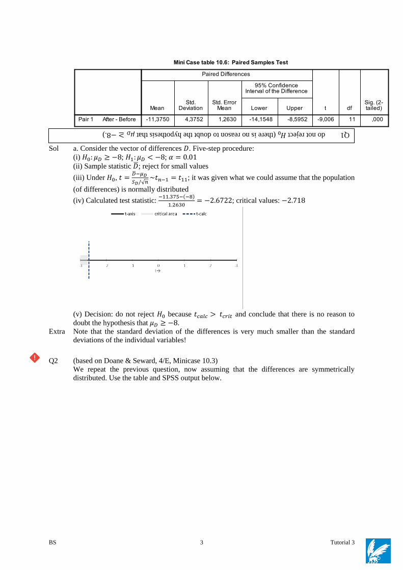
Sol a. Consider the vector of differences 𝐷. Five-step procedure:
(i) 𝐻0: 𝜇𝐷 ≥ −8; 𝐻1: 𝜇𝐷 < −8; 𝛼 = 0.01
(ii) Sample statistic ��; reject for small values
(iii) Under 𝐻0, 𝑡 =��−𝜇𝐷
𝑆𝐷/√𝑛~𝑡𝑛−1 = 𝑡11; it was given what we could assume that the population
(of differences) is normally distributed
(iv) Calculated test statistic: −11.375−(−8)
1.2630= −2.6722; critical values: −2.718
(v) Decision: do not reject 𝐻0 because 𝑡𝑐𝑎𝑙𝑐 > 𝑡𝑐𝑟𝑖𝑡 and conclude that there is no reason to
doubt the hypothesis that 𝜇𝐷 ≥ −8.
Extra Note that the standard deviation of the differences is very much smaller than the standard
deviations of the individual variables!
Q2 (based on Doane & Seward, 4/E, Minicase 10.3)
We repeat the previous question, now assuming that the differences are symmetrically
distributed. Use the table and SPSS output below.
Q1 do not reject 𝐻0 (there is no reason to doubt the hypothesis that 𝜇𝐷≥−8.)

BS 4 Tutorial 3
Legend: Column 1: data, Column 2: sorted data, Column 3: data −(−8), Column 4: remove
zeros, Column 5: assign ranks to absolute values and give signs (note: 1 and 2 are equal 1.5,
3 and 4 and 5 are equal 4), Column 6: add positive ranks, Column 7: count signs for sign
test.
Sol Problem: �� is no longer normally distributed because of the small sample size. Idea: subtract
−8 from all differences. Then replace observations by ranks of absolute values and add sign
according to larger or smaller.
(i) 𝐻0: 𝜇𝐷 ≥ −8; 𝐻1: 𝜇𝐷 < −8 (mean 𝜇 or median 𝑀, but symmetry is given); 𝛼 = 0.01
(ii) Sample statistic: 𝑊 (Sum of positive Ranks); reject for small values (make graph under
𝐻1!)
(iii) Distribution test statistic under 𝐻0: 𝑊~? . Use Signed-Ranks table for critical values from
distribution!
Requirements: Differences are symmetrically distributed
(iv) Calculated test statistic: 𝑊𝑐𝑎𝑙𝑐 = 8
Critical values: 10 (the smaller one! One-tailed test)
(v) Decision: do reject 𝐻0 (but it is close), because 𝑊𝑐𝑎𝑙𝑐 = 8 ≤ 𝑊𝑐𝑟𝑖𝑡 = 10. Conclude that
there is no evidence that the mean difference is larger than −8.
Extra Note: if no table available or if we state that normal approximation must be used:
H0: ME = -8 TRUE TRUE TRUE
TRUE TRUE
xi xi Xi - -8 Xi - -8 Rank(|.|) Sign Test
-14,5 -22,5 -14,5 -14,5 -12 -12 -1
-10 -15 -7 -7 -11 -11 -1
-15 -14,5 -6,5 -6,5 -10 -10 -1
-11 -12,5 -4,5 -4,5 -9 -9 -1
-9 -11 -3 -3 -7,5 -7,5 -1
-8,5 -11 -3 -3 -7,5 -7,5 -1
-11 -10 -2 -2 -6 -6 -1
-8,5 -9 -1 -1 -4 -4 -1
-7 -8,5 -0,5 -0,5 -1,5 -1,5 -1
-22,5 -8,5 -0,5 -0,5 -1,5 -1,5 -1
-7 -7 1 1 4 4 1
-12,5 -7 1 1 4 4 1
8 70 2 10
Signed Ranks
Test
Xi - ME Rank|..|
Signed Ranks
Sign |..|
N Mean Rank Sum of Ranks
After - Negative Ranks 10 a 7,00 70,00Before Positive Ranks 2 b 4,00 8,00
Ties 0 c
Total 12 a. After < Before
b. After > Before
c. After = Before
Ranks
After-
Before
Z -2,432 a
Asymp. Sig. (2-tailed) ,015
a. Based on positive ranks
b. Wilcoxon Signed Ranks Test
Test Statisticsb
Q2 do not reject 𝐻0 (there is no evidence that the mean difference is larger than −8.)

BS 5 Tutorial 3
(iii) Distribution (standardized) test statistic approximately under 𝐻0: 𝑊~𝑁(𝜇𝑊, 𝜎𝑊2 ) where
𝜇𝑊 =𝑛(𝑛+1)
4= 39 and 𝜎𝑊
2 =𝑛(𝑛+1)(2𝑛+1)
24= 162.5
Requirements: Differences are symmetrically distributed
(iv) Calculated test statistic: 𝑧𝑐𝑎𝑙𝑐 =8−39
√162.5= −2.4318; etc.
Q3 (based on Doane & Seward, 4/E, Minicase 10.3)
We repeat the previous two questions, now not assuming that the differences are symmetrically
distributed, and testing 𝐻0: 𝑀𝑑 ≥ −8. Use the table at Q3 and the SPSS output below.
Sol Problem: 𝑊 can no longer be used because of lack of symmetry. Idea: subtract −8 from all
differences. Then replace observations by plus or minus sign according to larger or smaller.
(i) 𝐻0: 𝑀𝐷 ≥ −8; 𝐻1: 𝑀𝐷 < −8; 𝛼 = 0.01
(ii) Sample statistic: 𝑋 (= # plusses); reject for small values (make graph!)
(iii) Distribution test statistic under 𝐻0: 𝑋~𝐵𝑖𝑛(12,0.5).
(iv) Calculated test statistic: 𝑋𝑐𝑎𝑙𝑐 = 2
𝑝-value of this statistical problem: 𝑃𝜋=0.5(𝑋 ≤ 2) = 0.0193
(v) Decision: do not reject 𝐻0, because 𝑝-value > 𝛼 = 0.01; conclude that there is no evidence
that the median difference is larger than −8.
6A Two 𝝁s or medians: comparisons
Q1 Shipments of meat, meat by-products, and other ingredients are mixed together in several filling
lines at a pet food factory. After the ingredients are thoroughly mixed, the pet food is placed in
eight-ounce cans. Descriptive statistics concerning fill weights from the two production Lines,
from two independent samples are given in the following table.
Assuming that the population variances are equal, at the 0.05 level of significance, is there
evidence of a difference between the mean weight of cans filled on the two lines?
Sol a. Use five steps with the equal-variance 𝑡-test.
(i) 𝐻0: 𝜇𝐴 = 𝜇𝐵 (where Populations: 1 = Line A, 2 = Line B) or 𝐻0: 𝜇𝐴 = 𝜇𝐵; 𝐻1: 𝜇𝐴 ≠ 𝜇𝐵 (𝛼 =0.05)
(ii) Sample statistic:𝑋1 − 𝑋2
. Reject for large and small values.
(iii) Distribution under 𝐻0: 𝑡 =(𝑋1 −𝑋2 )−(𝜇1−𝜇2)
√𝑆𝑝2(
1
𝑛1+
1
𝑛2)
~𝑡𝑛1+𝑛2−2 if we assume that population 1 is
normally distributed and population 2 is symmetrically distributed (‘equal variances’ is given).
(iv) 𝑡𝑐𝑎𝑙𝑐 =(𝑥1 −𝑥2 )−(𝜇1−𝜇2)
√𝑠𝑝2(
1
𝑛1+
1
𝑛2)
=(8.005−7.997)−0
√7.26×10⁻⁵(1
11+
1
16)
=0.008
0.003337= 2.3972
because 𝑠𝑃2 =
(𝑛1−1)𝑠12+(𝑛2−1)𝑠2
2
(𝑛1−1)+(𝑛2−1)=
10⋅(0.012)2+15⋅(0.005)2
10+15= 7.26 × 10⁻⁵
𝑡𝑐𝑟𝑖𝑡(25) = ±2.0595
Q3 do not reject 𝐻0 (there is no evidence that the median difference is larger than −8.)
Q1 Reject 𝐻0 (mean weight from line A is larger)

BS 6 Tutorial 3
(v) Decision rule: If 𝑡𝑐𝑎𝑙𝑐 < −2.0595 or 𝑡𝑐𝑎𝑙𝑐 > 2.0595, reject 𝐻0.
Since 𝑡𝑐𝑎𝑙𝑐 = 2.3972 > 2.0595 reject 𝐻0.
There is sufficient evidence of a difference in the mean weight of cans filled on the two lines.
Practical conclusion: mean weight from line A is larger (even if we have a two-sided test: reject
𝐻0 and give 1-sided practical conclusion).
Q2 The same problem as before, but now not assuming that the population variances are equal.
Sol Similar to Q1, except:
(iii) Distribution under 𝐻0: 𝑡 =(𝑋1 −𝑋2 )−(𝜇1−𝜇2)
√𝑆1
2
𝑛1+
𝑆22
𝑛2
~𝑡𝑑𝑓
Now, 𝑑𝑓 =(
𝑠12
𝑛1+
𝑠22
𝑛2)
2
(𝑠1
2
𝑛1)
2
𝑛1−1+
(𝑠2
2
𝑛2)
2
𝑛2−1
= 12.41, so use 𝑑𝑓 = 12
Requirements: assume that population 1 is normally distributed (𝑛1 < 15) and that population
2 is symmetrically distributed (𝑛2 = 16 > 15). (We make no further assumptions about the
variances)
(iv) Calculations:
𝑡𝑐𝑎𝑙𝑐 =(𝑥1 −𝑥2 )−(𝜇1−𝜇2)
√𝑠1
2
𝑛1+
𝑠22
𝑛2
=0.008
0.003828= 2.0899
𝑡𝑐𝑟𝑖𝑡(12) = ±2.1788
(v) Decision rule: use the approximation 𝑑𝑓 for the degrees of freedom in the 𝑡-distribution.
Since 𝑡𝑐𝑎𝑙𝑐 = 2.0899 < 2.1788 do not reject 𝐻0.
There is not sufficient evidence of a difference in the average weight of cans filled on the two
lines.
Q2 Do not reject 𝐻0 (there is not sufficient evidence of a difference in the average weight of
cans filled on the two lines)
BS 7 Tutorial 3
Extra Students have to be able to do this by hand and also from computer (SPSS) output!
Q3 Compare the results of the two previous questions.
Extra N.B. Equality of variances can be tested too (see later!).
It is essential that students are able to make this exercise with and without (SPSS) computer
output. (They should at least do the calculations once only from the table in the output!). In
exam papers we do not often ask to compute the degrees of freedom from the samples.
Q4 Same data as in Q1.
a. Assuming that the population variances are equal, find a 90% confidence interval for 𝜇𝐴 −𝜇𝐵.
b. Not assuming that the population variances are equal, find a 90% confidence interval for
𝜇𝐵 − 𝜇𝐴.
Sol a. Use: pooled variance
(𝑥𝐴 − 𝑥𝐵 ) ± 𝑡𝑑𝑓;0.05𝑠𝑋𝐴 −𝑋𝐵 = (8.005 − 7.997) ± 1.708 × 0.003337 → [0.002299,0.1370]
b. Use: separate variance
(𝑥𝐵 − 𝑥𝐴 ) ± 𝑡𝑑𝑓;0.05𝑠𝑋𝐴 −𝑋𝐵 = (7.997 − 8.005) ± 1.782 × 0.003828 →
[−0.01482, −0.001177]
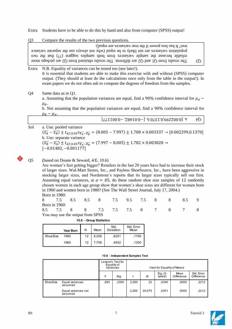
Q5 (based on Doane & Seward, 4/E, 10.6)
Are women’s feet getting bigger? Retailers in the last 20 years have had to increase their stock
of larger sizes. Wal-Mart Stores, Inc., and Payless ShoeSource, Inc., have been aggressive in
stocking larger sizes, and Nordstrom’s reports that its larger sizes typically sell out first.
Assuming equal variances, at 𝛼 = .05, do these random shoe size samples of 12 randomly
chosen women in each age group show that women’s shoe sizes are different for women born
in 1960 and women born in 1980? (See The Wall Street Journal, July 17, 2004.)
Born in 1980:
8 7.5 8.5 8.5 8 7.5 9.5 7.5 8 8 8.5 9
Born in 1960:
8.5 7.5 8 8 7.5 7.5 7.5 8 7 8 7 8
You may use the output from SPSS
Q3 The results from Q1 and Q2 are different. The results obtained from Q2 are perhaps more
reliable because the sample variances from both samples suggest (??) that the two
population variances are not likely to be equal (why not always use the separate variance
test? It has less power if the true variances are equal).
Q4 a. [0.002299,0.1370 b. [−0.01482,−0.001177]

BS 8 Tutorial 3
Sol Use the 5-steps procedure (including the assumptions)
Problem is two-sided with 𝛼 = 0.05 (although it was originally formulates as a one-sided
problem with 𝛼 = 0.025)
(i) 𝐻0: 𝜇1 = 𝜇2 (where Populations: 1 = 1980, 2 = 1960) or 𝐻0: 𝜇1980 − 𝜇1960 = 0 (Mean shoe
size is the same.)
𝐻1: 𝜇_1 ≠ 𝜇2 (𝛼 = 0.05)
(ii) Sample statistic: 𝑋1 − 𝑋2
; reject for large and small values.
(iii) Distribution under 𝐻0: 𝑡 =(𝑋1 −𝑋2 )−(𝜇1−𝜇2)
√𝑆𝑃2(
1
𝑛1+
1
𝑛2)
~𝑡𝑛1+𝑛2−2 = 𝑡22 (see output)
Requirements: both populations should be normally distributed (both 𝑛 < 15)
(iv) Computations:
𝑠𝑃2 =
(𝑛1−1)𝑠12+(𝑛2−1)𝑠2
2
(𝑛1−1)+(𝑛2−1)=
11(0.6201)2+11(0.4502)2
11+11= 0.2936
𝑠𝑃2 (
1
𝑛1+
1
𝑛2) = 0.2936 × (
1
12+
1
12) = 0.04893 = (0.2212)2
𝑡𝑐𝑎𝑙𝑐 =(8.208−7.708)−0
0.2212= 2.260
𝑝-value = 0.0340 (see output)
(v) 𝑝-value = 0.0340 < 5%, so reject 𝐻0.
Decision: Since 𝑡𝑐𝑎𝑙𝑐 = 2.260 is outside the lower and upper critical bound of −2.074 and
2.074, do reject 𝐻0. There is enough evidence to conclude that the mean shoe size is different.
One-sided ‘Post Hoc conclusion’: Shoe Size has increased.
Q6 (based on Doane & Seward, 4/E, 16.B-2)
Q5 Reject 𝐻0 (there is enough evidence to conclude that the mean shoe size has increased)

BS 9 Tutorial 3
Below are data for two different regions, showing the number of days that kidney transplant
patients had to wait before a donor was found (𝑛𝐸 = 6 patients, 𝑛𝑊 = 8 patients).
East: 109 248 85 107 28 67
West: 137 93 52 191 236 205 92 133
Do not assume a normal distribution of waiting times.
Use Table 16.B1 to test the hypothesis of equal medians at 𝛼 = .05 Show the steps in your
analysis.
Sol Replace data by ranks: combine samples, rank them, and put ranks back in original sample.
(i) 𝐻0: 𝑀𝐸 = 𝑀𝑊; 𝐻1: 𝑀𝐸 ≠ 𝑀𝑊 (𝛼 = 5%)
(ii) Sample statistic: 𝑇𝐸 (sum of ranks from sample smallest sample, so from East); reject for
large and small values
(iii) Distribution test statistic under 𝐻0: directly from ‘Wilcoxon’ table
Requirements: both distributions have similar shape
(iv) Calculated test statistic: The ranks for (smallest) sample (so sample 𝐸) are 1, 3, 4, 7, 8 and
14, respectively; 𝑇𝐸 = 37 (so 𝑇𝑊 = 105 − 37 = 68).
Critical values: 𝑛𝐸 = 6, 𝑛𝑊 = 8, 𝑇𝐸(𝑐𝑟𝑖𝑡, 𝐿) = 29, 𝑇𝐸(𝑐𝑟𝑖𝑡, 𝑅) = 61
(v) Decision: do not reject 𝐻0 because 𝑇𝐸 not in critical region; conclude there is no reason to
doubt the equality of the medians (or the means, because of similar shape of both distributions)
Q7 (based on Doane & Seward, 4/E, 16.B-2)
Use the data from Q6 and 𝛼 = 5%.
a. Test 𝐻0: 𝑀𝑊 ≤ 𝑀𝐸 against 𝐻1: 𝑀𝑊 > 𝑀𝐸 (where 𝑀 is median), using the tables on the
website
b. Use the normal approximation to answer the same question. Is your conclusion the same?
Sol a. 𝐻0: 𝑀𝑊 ≤ 𝑀𝐸 vs. 𝐻1: 𝑀𝑊 > 𝑀𝐸, but we prefer to write 𝐻0: 𝑀𝐸 ≥ 𝑀𝑊 vs. 𝐻1: 𝑀𝐸 < 𝑀𝑊
(smallest sample first and take statistic 𝐸1). Reject for small values of 𝑇𝐸
(iv) Critical values: 𝑛𝐸 = 6, 𝑛𝑊 = 8, 𝑇𝐸(𝑐𝑟𝑖𝑡) = 31
(v) Decision: do not reject 𝐻0 because 𝑇𝐸 > 31
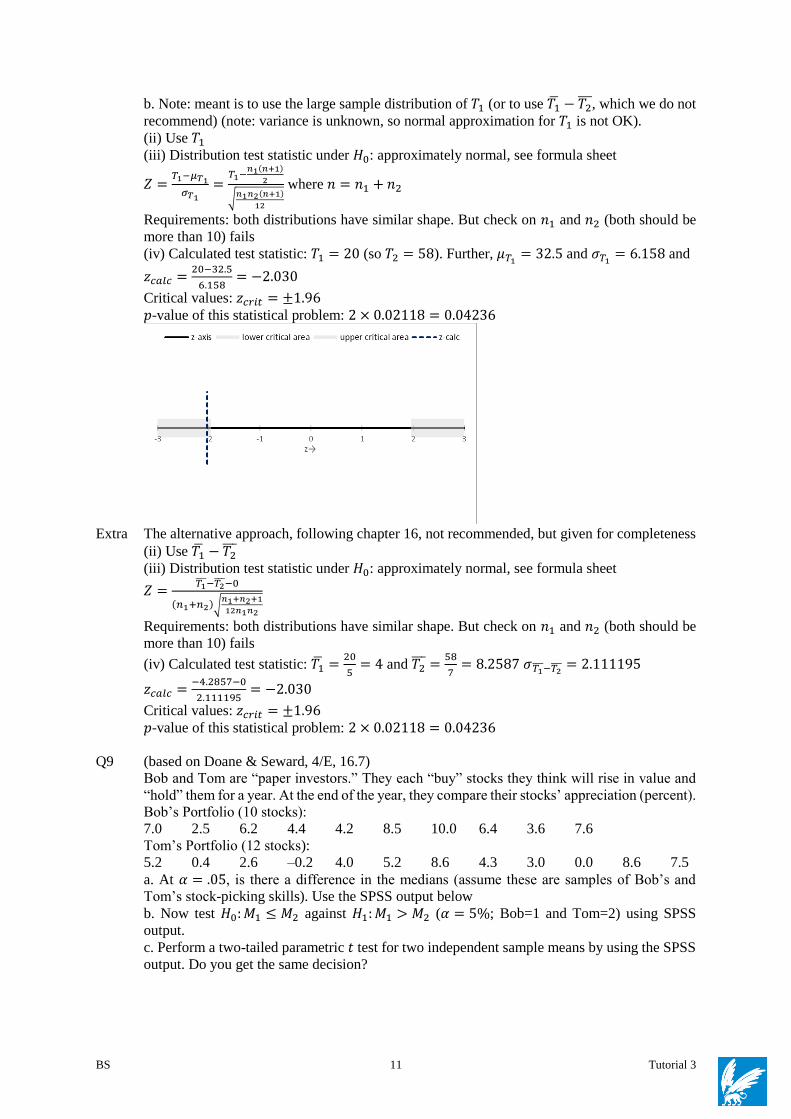
b. Note: meant is to use the large sample distribution of 𝑇𝐸 (small sample, so normal
approximation for 𝑇𝐸 is not OK).
(ii) Sample statistic 𝑇𝐸; reject for small values
(iii) Distribution test statistic under 𝐻0: approximately normal, see formula sheet
𝑍 =𝑇𝐸−𝜇𝑇𝐸
𝜎𝑇𝐸
=𝑇𝐸−
𝑛𝐸(𝑛+1)
2
√𝑛𝐸𝑛𝑊(𝑛+1)
12
where 𝑛 = 𝑛𝐸 + 𝑛𝑊
Requirements: both distributions have similar shape. But check on 𝑛𝐸 and 𝑛𝑊 (both should be
more than 10) fails
(iv) Calculated test statistic:
𝑇𝐸 = 37 (so 𝑇𝑊 = 68). Further 𝜇𝑇𝐸= 45 and 𝜎𝑇𝐸
= 7.7460; 𝑧𝑐𝑎𝑙𝑐 =37−45
7.7460= −1.0328
Critical values: 𝑧𝑐𝑟𝑖𝑡 = −1.645
Q6 do not reject 𝐻0 (no reason to doubt the equality of the medians or means)
Q7 do not reject 𝐻0 (no reason to doubt that 𝑀𝑊≤𝑀𝐸)

BS 10 Tutorial 3
𝑝-value of this statistical problem: 0.1508
(v) Do not reject 𝐻0, and conclude that there is no reason to doubt that 𝑀𝑊 ≤ 𝑀𝐸
Q8 (based on Doane & Seward, 4/E, 16.B-1)
A trucking company wants to compare the number of miles driven by two delivery truck drivers
in one week on different days (𝑛1 = 5 days, 𝑛2 = 7 days). Do not assume that distances driven
are normally distributed.
Driver 1: 128 102 78 40 76
Driver 2: 97 158 112 112 216 316 112
a. Use Table 16.B1 to test the hypothesis of equal medians at 𝛼 = .05. Show the steps in your
analysis.
b. Perform a large-sample test using a normal approximation for the distribution of 𝑇1. Is your
conclusion the same?
Sol Replace data by ranks: combine samples, rank them, and put ranks back in original sample.
a. Five steps:
(i) 𝐻0: 𝑀1 = 𝑀2; 𝐻1: 𝑀1 ≠ 𝑀2 (𝛼 = 5%)
(ii) Sample statistic: 𝑇1 (=sum of ranks from sample ‘Driver 1’); reject for large and small
values
Use 16.9 from Doane 4th edition.
(iii) Distribution test statistic under 𝐻0: directly from ‘Wilcoxon’ table
Requirements: both distributions have similar shape
(iv) Calculated test statistic: The ranks for (smallest) sample 1 are 1, 2, 3, 5 and 9, respectively;
𝑇1 = 20 (so 𝑇2 = 78 − 20 = 58).
Critical values: 𝑛1 = 5, 𝑛2 = 7, 𝑇1(𝑐𝑟𝑖𝑡, 𝐿) = 20 and 𝑇1(𝑐𝑟𝑖𝑡,𝑅) = 45
(v) Decision: reject 𝐻0 because 𝑇1 in the critical region (on the border) and conclude (but be
careful) that there is reason to doubt the equality of the medians or the means (if assumption of
similar shape of both distributions is reasonable)
Driver 1 Driver 2
128 9
102 5
78 3
40 1
76 2
97 4
158 10
112 7
112 7
216 11
316 12
112 7
20 58
Wilcoxon - Mann/Whitney Test
n sum of ranks
5 20 Driver 1
7 58 Group 2
12 78 total
32,500 expected value
6,158 standard deviation
-2,030 z
,0424 p-value (two-tailed)
Q8 reject 𝐻0 (there is reason to doubt the equality of the medians or means)
BS 11 Tutorial 3
b. Note: meant is to use the large sample distribution of 𝑇1 (or to use 𝑇1 − 𝑇2, which we do not
recommend) (note: variance is unknown, so normal approximation for 𝑇1 is not OK).
(ii) Use 𝑇1
(iii) Distribution test statistic under 𝐻0: approximately normal, see formula sheet
𝑍 =𝑇1−𝜇𝑇1
𝜎𝑇1
=𝑇1−
𝑛1(𝑛+1)
2
√𝑛1𝑛2(𝑛+1)
12
where 𝑛 = 𝑛1 + 𝑛2
Requirements: both distributions have similar shape. But check on 𝑛1 and 𝑛2 (both should be
more than 10) fails
(iv) Calculated test statistic: 𝑇1 = 20 (so 𝑇2 = 58). Further, 𝜇𝑇1= 32.5 and 𝜎𝑇1
= 6.158 and
𝑧𝑐𝑎𝑙𝑐 =20−32.5
6.158= −2.030
Critical values: 𝑧𝑐𝑟𝑖𝑡 = ±1.96
𝑝-value of this statistical problem: 2 × 0.02118 = 0.04236
Extra The alternative approach, following chapter 16, not recommended, but given for completeness
(ii) Use 𝑇1 − 𝑇2
(iii) Distribution test statistic under 𝐻0: approximately normal, see formula sheet
𝑍 =𝑇1 −𝑇2 −0
(𝑛1+𝑛2)√𝑛1+𝑛2+1
12𝑛1𝑛2
Requirements: both distributions have similar shape. But check on 𝑛1 and 𝑛2 (both should be
more than 10) fails
(iv) Calculated test statistic: 𝑇1 =20
5= 4 and 𝑇2
=58
7= 8.2587 𝜎𝑇1 −𝑇2 = 2.111195
𝑧𝑐𝑎𝑙𝑐 =−4.2857−0
2.111195= −2.030
Critical values: 𝑧𝑐𝑟𝑖𝑡 = ±1.96
𝑝-value of this statistical problem: 2 × 0.02118 = 0.04236
Q9 (based on Doane & Seward, 4/E, 16.7)
Bob and Tom are “paper investors.” They each “buy” stocks they think will rise in value and
“hold” them for a year. At the end of the year, they compare their stocks’ appreciation (percent).
Bob’s Portfolio (10 stocks):
7.0 2.5 6.2 4.4 4.2 8.5 10.0 6.4 3.6 7.6
Tom’s Portfolio (12 stocks):
5.2 0.4 2.6 –0.2 4.0 5.2 8.6 4.3 3.0 0.0 8.6 7.5
a. At 𝛼 = .05, is there a difference in the medians (assume these are samples of Bob’s and
Tom’s stock-picking skills). Use the SPSS output below
b. Now test 𝐻0: 𝑀1 ≤ 𝑀2 against 𝐻1: 𝑀1 > 𝑀2 (𝛼 = 5%; Bob=1 and Tom=2) using SPSS
output.
c. Perform a two-tailed parametric 𝑡 test for two independent sample means by using the SPSS
output. Do you get the same decision?

BS 12 Tutorial 3
Sol Replace data by ranks: combine samples, rank them, and put ranks back in original sample.
Note: no table available.
Do the test using the computer output (new for them) and only the one-sided (extra) question.
a. Five steps:
(i) 𝐻0: 𝑀1 = 𝑀2; 𝐻1: 𝑀1 ≠ 𝑀2; 𝛼 = 5% (Bob=1, Tom=2)
(ii) Sample statistic: 𝑇1 (sum of ranks from sample ‘Bob’); reject for large and small values
(iii) Distribution test statistic under 𝐻0: approximately normally distributed (parameters
depending on choice in step (ii)
Requirements: both distributions have similar shape. Check on 𝑛1 and 𝑛2: both at least 10, so
approximation should be OK
(iv) Calculated test statistic: 𝑧𝑐𝑎𝑙𝑐 = −1.320
Reported 𝑝-value: 0.187; 𝑝-value of this statistical problem: 0.187
Q9 do not reject 𝐻0 (no reason to doubt the equality of the medians or means)

BS 13 Tutorial 3
(v) Decision: do not reject 𝐻0 because 𝑝-value > 5% and conclude there is no reason to doubt
the equality of the medians or the means (!!!!, because of similar shape of both distributions).
b. To test 1-sided hypothesis: look at mean ranks!
(i) 𝐻0: 𝑀1 ≤ 𝑀2; 𝐻1: 𝑀1 > 𝑀2 (𝛼 = 5%)
(iv) Calculated test statistic: 𝑧𝑐𝑎𝑙𝑐 = −1.320, but sign is meaningless (!!!)
Because MeanRanks(1) > MeanRanks(2) in sample, we are close to rejection region (whatever
statistic we might have chosen).
So 𝑝-value = 0.5 × 𝑝-twosided =0.187
2= 0.093
c. Steps that change:
(iii) Distribution test statistic under 𝐻0: 𝑡~𝑡20
Requirements: both distributions are normal, equal variance (latter is reasonable assumption in
Levene’s test: 𝑝-value = 39.6%)
(v) Decision: do not reject 𝐻0 because 𝑝-value = 0.121 > 5% and conclude there is no reason
to doubt the equality of the means
6B Two 𝝈𝟐s: comparisons
Q1 (Doane & Seward, 4/E, 10.39)
A manufacturing process drills holes in sheet metal that are supposed to be . 5000 cm in
diameter. Before and after a new drill press is installed, the hole diameter is carefully measured
(in cm) for 12 randomly chosen parts. At 𝛼 = .05, do these independent random samples prove
that the new process has smaller variance? Show the hypotheses, decision rule, and test statistic.
Sol (i) 𝐻0: 𝜎1
2 ≤ 𝜎22; 𝐻1: 𝜎1
2 > 𝜎22 (where 1=Old, 2=New) (‘Old’ in numerator for easy critical
value)
(ii) Test Statistic: 𝐹 =𝑆1
2
𝑆22. Reject for large values
(iii) Under 𝐻0: 𝐹~𝐹11;11
Requirement: both populations normal
(iv) Test statistic: 𝐹𝑐𝑎𝑙𝑐 =𝑠1
2
𝑠22 =
3.183×10⁻⁵
3.265×10−6 = 9.748 (see output below)
Critical values: 𝐹𝑐𝑟𝑖𝑡(11; 11; 0.05) = 2.82
Q1 reject 𝐻0 (the new drill has a significantly smaller variance)

BS 14 Tutorial 3
(v) Decision: Since 𝐹𝑐𝑎𝑙𝑐 = 9.748 is above the critical bound of 2.82 do reject 𝐻0. There is
enough evidence to conclude that the new drill has reduced variance.
Compare the two Excel outputs, one with the smallest in the numerator (so 𝐹𝑐𝑎𝑙𝑐 < 1), the other
with the largest in the numerator (so 𝐹𝑐𝑎𝑙𝑐 > 1).
Extra Excel produces the following two tables, with left 1=new, 2=old, and right 1=old, 2=new. There
is an error in Excel in the second table: the “<=” should be “>=”.
Q2 (Doane & Seward, 4/E, 10.40)
Examine the data below showing the weights (in pounds) of randomly selected checked bags
for an airline’s flights on the same day.
a. At 𝛼 = .05, is the mean weight of an international bag greater? Show the hypotheses,
decision rule, and test statistic.
b. At 𝛼 = .05, is the variance greater for bags on an international flight? Show the hypotheses,
decision rule, and test statistic.
Use the output below:
F-Test Two-Sample for Variances
New Drill Old Drill
Mean 0,5002167 0,5000167
Variance 3,265E-06 3,183E-05
Observations 12 12
df 11 11
F 0,1025849
P(F<=f) one-tail 0,0003546
F Critical one-tail 0,3548704
F-Test Two-Sample for Variances
Old Drill New Drill
Mean 0,5000167 0,5002167
Variance 3,183E-05 3,265E-06
Observations 12 12
df 11 11
F 9,7480278
P(F<=f) one-tail 0,0003546
F Critical one-tail 2,8179305

BS 15 Tutorial 3
Sol a. First test the equality of variances in order to choose between equal and unequal variance 𝑡-
test. The 𝑝-value is 0.000887, so we reject the hypothesis of equal variance, and start using the
𝑡-test not assuming equal variances.
Note: as an exercise for the 𝐹-test, we do this below for a full 5-step procedure. At the exam,
this is not needed when we ask for testing the equality of two means.
(i) 𝐻0:𝜎1
2
𝜎22 = 1; 𝐻1:
𝜎12
𝜎22 ≠ 1; 𝛼 = 0.05 (with 1=international, 2=domestic)
(ii) Test Statistic: 𝐹 =𝑆1
2
𝑆22; reject for small and large values
(iii) Under 𝐻0: 𝐹~𝐹9;14
Requirement: both populations normal.
(iv) Test statistic: 𝐹𝑐𝑎𝑙𝑐 =𝑠1
2
𝑠22 =
141.3778
20.98095= 6.738 (see output above)
Critical values: 𝐹𝑐𝑟𝑖𝑡,𝑅 = 𝐹9;14;0.025 = 3.21 and 𝐹𝑐𝑟𝑖𝑡,𝐿 = 𝐹9;14;0.975 = ⋯ (It is not necessary to
find 𝐹𝑐𝑟𝑖𝑡,𝐿.
t-Test: Two-Sample Assuming Equal Variances
International Domestic
Mean 48,6 36,13333
Variance 141,3778 20,98095
Observations 10 15
Pooled Variance 68,09275
Hypothesized Mean Difference 0
df 23
t Stat 3,700629
P(T<=t) one-tail 0,00059
t Critical one-tail 1,713872
P(T<=t) two-tail 0,001179
t Critical two-tail 2,068658
t-Test: Two-Sample Assuming Unequal Variances
International Domestic
Mean 48,6 36,13333
Variance 141,3778 20,98095
Observations 10 15
Hypothesized Mean Difference 0
df 11
t Stat 3,162814
P(T<=t) one-tail 0,004517
t Critical one-tail 1,795885
P(T<=t) two-tail 0,009034
t Critical two-tail 2,200985
F-Test Two-Sample for Variances
International Domestic
Mean 48,6 36,13333
Variance 141,3778 20,98095
Observations 10 15
df 9 14
F 6,738387
P(F<=f) one-tail 0,000887
F Critical one-tail 2,645791
Q2 a. Reject 𝐻0 (the mean of international bag weight is greater than domestic bag weight)
b. Reject 𝐻0 (the variance of international bag weight is greater than domestic bag weight.)

BS 16 Tutorial 3
(v) Decision: Since 𝐹𝑐𝑎𝑙𝑐 = 6.738 is above the critical bound of 3.21 do reject 𝐻0. There is
enough evidence to conclude that the variances are not equal.
So we have to use the ‘separate variance 𝑡-test for the µ-problem.
(Post-hoc: the variance for international is larger)
Now we test the question from a.
(i) 𝐻0: 𝜇1 − 𝜇2 ≤ 0; 𝐻1: 𝜇1 − 𝜇2 > 0 (𝛼 = 0.05)
(ii) Test statistic: 𝑋1 − 𝑋2
; reject for large values
(iii) Under 𝐻0: 𝑡 =(𝑋1 −𝑋2 )−(𝜇1−𝜇2)
√𝑆1
2
𝑛1+
𝑆22
𝑛2
~𝑡𝑑𝑓 where 𝑑𝑓 =(
𝑠12
𝑛1+
𝑠22
𝑛2)
2
(𝑠1
2
𝑛1)
2
𝑛1−1+
(𝑠2
2
𝑛2)
2
𝑛2−1
(from output: 𝑑𝑓 = 11)
Requirements: assume that population 1 is normally distributed (𝑛1 < 15) and population 2 is
symmetrically distributed (𝑛2 = 15 ≥ 15).
(iv) Calculations:
𝑡𝑐𝑎𝑙𝑐 =(𝑥1 −𝑥2 )−(𝜇1−𝜇2)
√𝑠1
2
𝑛1+
𝑠22
𝑛2
=(48.6−36.13333)−0
√141.3778
10+
20.98095
15
=12.46667
3.941638= 3.162814
𝑡𝑐𝑟𝑖𝑡 = 𝑡11;0.05 = 1.796 (from table; from output: 1.795885)
(Note: 𝑡𝑐𝑎𝑙𝑐 bot drawn to scale)
(v) Since 𝑡𝑐𝑎𝑙𝑐 = 3.163 > 1.796 or (from output) 𝑝-value = 𝑃(𝑡11 > 3.162814) =0.004517 < 0.05, reject 𝐻0. The mean of international bag weight is greater than domestic bag
weight.
b. Now test variances
(i) 𝐻0:𝜎1
2
𝜎22 ≤ 1; 𝐻1:
𝜎12
𝜎22 > 1; (𝛼 = 0.05)
(ii) Test Statistic: 𝐹 =𝑆1
2
𝑆22; reject for large values
(iii) Under 𝐻0: 𝐹~𝐹9;14
Requirements: both populations normal.
(iv) Test statistic: 𝐹𝑐𝑎𝑙𝑐 =𝑠1
2
𝑠22 =
141.3778
20.98095= 6.738 (see output above)

BS 17 Tutorial 3
Critical value: 𝐹𝑐𝑟𝑖𝑡;𝑅 = 𝐹9;14;0.05 = 2.65; 𝐹𝑐𝑟𝑖𝑡;𝐿 not needed
(v) Decision rule: Reject 𝐻0 if 𝐹𝑐𝑎𝑙𝑐 ≥ 2.65 and 𝐹𝑐𝑎𝑙𝑐 = 6.7387 so we reject the null
hypothesis. The variance of international bag weight is greater than domestic bag weight.
Note: From output: 𝑝-value = 𝑃(𝐹9;14 ≥ 6.7387) = 0.000887 < 0.05
Q3 (based on Doane & Seward, 4/E, 10.6)
At the tests for comparing two 𝜇s above, we analyzed the change of foot size of women. Now
test the equality of variance at 𝛼 = 5%.
a. Use the usual variance test, with a full calculation.
b. Use the SPSS output, without a full calculation.
Data are repeated below:
Born in 1980:
8 7.5 8.5 8.5 8 7.5 9.5 7.5 8 8 8.5 9
Born in 1960:
8.5 7.5 8 8 7.5 7.5 7.5 8 7 8 7 8
Sol On the basis of the usual variance test
(i) 𝐻0: 𝜎12 = 𝜎2
2; 𝐻1: 𝜎12 ≠ 𝜎2
2 (where Populations: 1 = 1980, 2 = 1960); 𝛼 = 0.05
(ii) Sample statistic: 𝐹 =𝑆1
2
𝑆22; reject for large and for small small values
(iii) Distribution under 𝐻0: 𝐹 =𝑠1
2
𝑠22 ~𝐹11;11
Requirements: Both populations normally distributed
(iv) Computations: 𝐹𝑐𝑎𝑙𝑐 =(0.6201)2
(0.4502)2 = 1.8972
𝐹𝑐𝑟𝑖𝑡;𝑅 = 𝐹11,11;0.025 = 3.47 (not in table) and 𝐹𝑐𝑟𝑖𝑡;𝐿 < 1
Note: from table 𝐹𝑐𝑟𝑖𝑡 between 3.53 and 3.43.
Q2 Do not reject 𝐻0 (the two variances do not differ significantly)

BS 18 Tutorial 3
(v) Do not reject 𝐻0. because 𝐹𝑐𝑎𝑙𝑐 not in rejection region. Variances do not differ significantly.
Using SPSS output, you can use the Levene’s test instead:
(i) identical
(ii) Sample statistic: Levene’s 𝐹; (reject for large values)
(iii) Distribution under 𝐻0: 𝐹~? ? ? (now see SPSS output). This test is a two-sided but one-
tailed test!
Requirements: ???
(iv) Computations: 𝐹𝑐𝑎𝑙𝑐 = 0.993 (see output) and 𝑝-value 0.3300
(v) Do not reject 𝐻0 because 𝑝-value larger than 5%.
Old exam questions
Q1 23 March 2016, Q3a
It has been suggested that students perform differently in the afternoon compared to the
morning. To investigate this phenomenon, a number of tests have been made: 12 randomly
chosen students did an exam in the morning, and 12 others did an exam in the afternoon. The
results of the exams are on a scale from 1.0 (low) to 10.0 (high). One group of researchers
proposes to compare the mean score in the morning to the mean score in the afternoon. Perform
this test at 𝛼 = 5%, using the 5-step procedure.
Sol This is a case of comparing the means of two independent samples.
(i) 𝐻0: 𝜇1 = 𝜇2, 𝐻1: 𝜇1 ≠ 𝜇2, 𝛼 = 0.05 (where 1 codes for morning and 2 for afternoon)
(ii) Sample statistic: 𝑋1 − 𝑋2
, reject for small and for large values
(iii) null distribution: 𝑋1 −𝑋2
𝑆𝑋1 −𝑋2 ~𝑡22, provided both populations are normally distributed (which
we will have to assume) and the two populations have the same variance (which looks quite
plausible, given Levene’s test with 𝑝-value = 0.976)
(iv) 𝑡𝑐𝑎𝑙𝑐 = 1.410, 𝑡𝑐𝑟𝑖𝑡 = ±2.074, 𝑝-value = 0.172
(v) do not reject 𝐻0, there is no evidence for concluding that the population means are different
Q2 22 May 2017, Q3d
Electricity supply is a vital element for nearly every part of the economy. Supply must be stable:
voltage should be 230 volt and variations must be small. We measure at 21 random times in
The Netherlands (NL) and at 26 random times in Germany (DE) voltage and find the following
descriptive statistics:
Q1 Do not reject 𝐻0 (there is no evidence for concluding that the population means are different)

BS 19 Tutorial 3
Use the data above to test if the assumption 𝜎𝑁𝐿
2 = 𝜎𝐷𝐸2 is reasonable, at 𝛼 = 5%. Calculate the
value of the test statistic, as well as the critical value(s). Make assumptions and state
requirements where needed and/or check requirements where possible.
Sol The standardized test statistic for comparing two variances is 𝐹 =𝑆𝑁𝐿
2
𝑆𝐷𝐸2 . Its observed value is
1.306 (or 0.766 in case you define 𝐹 =𝑆𝐷𝐸
2
𝑆𝑁𝐿2 ).
Under the null hypothesis, this test statistic is distributed as 𝐹𝑛𝑁𝐿−1,𝑛𝐷𝐸−1 (or 𝐹𝑛𝐷𝐸−1,𝑛𝑁𝐿−1).
The test is two-sided. Critical values are thus 𝐹𝑐𝑟𝑖𝑡,𝑢𝑝𝑝𝑒𝑟 = 𝐹20,25;0.025 = 2.30 and
𝐹𝑐𝑟𝑖𝑡,𝑙𝑜𝑤𝑒𝑟 =1
𝐹25,20;0.025=
1
2.40= 0.42. (Or if you used the other definition of 𝐹: 2.40 and
1
2.30=
0.43)
The requirement is that both populations (NL and DE) are normal; this seems reasonable given
the estimated values of skewness and kurtosis for both NL and DE (should be between −1 and
1).
Q2 𝐹𝑐𝑎𝑙𝑐=1.306; 𝐹𝑐𝑟𝑖𝑡=2.30 and 0.42; both populations must be normal, which is OK.