Buyer Power and Quality Improvements�

Pierpaolo Battigalli, Chiara Fumagalli, Michele Polo

Bocconi University

Abstract

This paper analyses the sources of buyer power and its e¤ect on sellers�

investment in quality improvements. In our model retailers make take-

it-or-leave-it o¤ers to a producer and each of them obtains its marginal

contribution to total pro�ts (gross of sunk costs). In turn, this depends on

the rivalry between retailers in the bargaining process. Rivalry increases

when the retailers are less di¤erentiated and when decreasing returns to

scale in production are larger. The allocation of total surplus a¤ects the

incentives of the producer to invest in product quality, an instance of the

hold-up problem. An increase in buyer power not only makes the supplier

and consumers worse o¤, but it may even harm the retailers, that obtain

a larger share of a smaller surplus. A repeated game argument shows that

e¢ cient quality improvements can be supported as an equilibrium outcome

if producer and retailers are involved in a long-term relationship.

KEYWORDS: Buyer power; Non-cooperative Bargaining, Hold-up.

J.E.L. CLASSIFICATION NUMBERS: L13, L4.

�Corresponding author: Chiara Fumagalli, Bocconi University, Via Sarfatti, 25, 20136 Milan,Italy, chiara.fumagalli@unibocconi.it. We would like to thank Roman Inderst, Massimo Motta,Marco Ottaviani, Helder Vasconcelos and Lucy White for helpful comments on an earlier draft.Financial support from Centromarca is gratefully acknowledged.

1 Introduction

In the last decades, the retailing sector - in particular grocery retailing - has

experienced a movement towards increased concentration. Broadly speaking, large

retail chains and multinational retail companies (such as Wal-Mart, Carrefour,

the Metro group) now play a dominant role, even though the phenomenon is

not uniform across countries.1 At the EU level, retailer concentration is further

strengthened by purchasing alliances (operating nationally or cross-border such

as Euro Buying or Buying International Group). Buyer power is on the rise also

in other industries, such as automobile,2 healthcare and cable television (in the

US).3

These trends have triggered investigations by anti-trust agencies and policy

institutions around the world on the e¤ects of increasing buyer power.4 One

concern that is often expressed is that excessive buyer power may deteriorate

suppliers� incentive by squeezing their pro�t margins and thus indirectly harm

consumers and overall welfare. For instance, according to the FTC report, "even if

consumers receive some bene�ts in the short run when retailers use their bargaining

leverage to negotiate a lower price, they could be adversely a¤ected by the exercise

of buyer power in the longer run, if the suppliers respond by under-investing in

innovation or production" (FTC 2001, p.57).

In this paper we formalize this argument by studying the impact of buyer

power on a supplier�s incentive to improve quality.

Our model assumes a monopolistic producer and two independent retailers.

First, the supplier chooses to improve the (non-contractible) quality of its product

through a sunk investment. Higher quality makes �nal consumers more willing to

pay for the good, thereby increasing total industry pro�ts (gross of sunk costs). Af-

1For example, in the UK supermarkets accounted for 20% of grocery sales in 1960, but 89% in2002, with the top-5 stores controlling 67% of all sales. France exhibits similar features. In othercountries, such as Italy and the US, small independent retailers still retain a strong position inthe market, although their position has eroded over time. Moreover, in the US the supermarketindustry is experiencing an unprecedented merger wave. For an overview of recent changes inthe retail sector see Dobson and Waterson (1999), Dobson (2005) and OECD (1999).

2The increased bargaining power of automakers when negotiating with parts suppliers isdocumented, among the others, by Peters (2000).

3In cable television, the concern of excessive buyer power of MSO (multiple system operators)is one of the reasons why the FTC has enforced legal restrictions on their size. See Raskovich(2003) and Chae and Heidhues (2004). In the healthcare sector, buyers (drugstores, hospitalsand HMOs) aggregate into large procurement alliances in order to reduce prescription drug costs.See Ellison and Snyder (2002) and DeGraba (2005).

4The growing concern about buyer power is documented in the Symposium on Buyer Powerand Antitrust, Antitrust Law Journal (2005). See also Dobson and Waterson (1999), Rey (2000)and the reports by OECD (1999), FTC (2001), EC (1999).

1

ter the quality decision, supply conditions are determined in bilateral negotiations.

While most of the literature on buyer power employs speci�c cooperative solution

concepts, we explicitly specify a non-cooperative bargaining protocol. This al-

lows us to precisely identify how fundamentals (preferences and technology) a¤ect

buyer power. We consider the simplest bargaining setting in which buyer power

and its sources can be analyzed. In particular, we assume that retailers make

(simultaneous) take-it-or-leave-it o¤ers to the producer, with no restrictions on

the type of contracts that can be o¤ered.

The solution of the negotiation game - given the quality choice - provides the

following insights. Firstly, in equilibrium total industry gross pro�ts are maxi-

mized. This is obtained, absent any restriction on contractual forms, as an out-

come of the negotiation process. Secondly, total industry pro�ts are distributed

so that each retailer receives its marginal contribution, i.e. the additional surplus

created when one more retailer is supplied. In turn, retailers�marginal contribu-

tion is determined by demand and supply conditions. Let us consider �rst the

demand channel. If retailers are perceived as perfectly substitutable by �nal con-

sumers (because there is neither geographical di¤erentiation nor di¤erentiation in

the provision of sale services), the maximum industry pro�t can be achieved by

supplying one retailer only. Hence, the marginal contribution of each retailer is

zero, and the supplier appropriates the entire surplus from the negotiation, even

though retailers make take-it-or-leave-it o¤ers. Di¤erently stated, this case ex-

hibits the strongest rivalry among retailers in the negotiation with the supplier.

As retailers�di¤erentiation increases, their marginal contribution increases as well

(and rivalry weakens). Thus, the share of total pro�ts they absorb in the negoti-

ation increases.

The second source of rivalry comes from the supply channel, through the con-

vexity of the producer�s cost function. With an increasing marginal cost curve

the two retailers compete for the productive resources of the supplier. If a retailer

increases its sales, it causes an increase in the marginal cost incurred to supply

the other retailer, and therefore reduces the marginal pro�ts created by the latter.

A steeper marginal cost curve enhances this "congestion" e¤ect.

We then analize the quality choice made by the producer. Buyer power, by

reducing the share of total pro�ts that the supplier extracts from the negotiation,

weakens the producer�s incentive to engage in quality improvement, an instance of

the hold-up problem. Hence, it makes both the producer and �nal consumers worse

o¤. Furthermore, we identify conditions under which an increase in buyer power

turns out to harm also the retailers, because the "smaller-cake e¤ect" dominates

2

the "larger-slice" one.

Finally, we show that repeated interaction may induce the producer to choose

the e¢ cient quality level even in the presence of powerful buyers.

Related literature This paper relates to the growing literature on buyer power.

This literature has addressed three main issues: (i) why larger buyers obtain better

deals from sellers; (ii) whether wholesale discounts obtained by large buyers are

passed on to �nal consumers; (iii) what are the implications of buyer power for

suppliers�incentives.

The literature exploring the sources of buyer power is very heterogeneous.5 ;6 In

a number of papers, size discounts arise because large buyers are better bargainers

than small ones. This occurs for various reasons. Larger buyers can distribute the

costs to generate alternative supply options over a larger number of units. This

makes their threat to integrate backwards credible and improves their bargaining

position with the supplier (Katz, 1987; Inderst and Wey, 2005b). In Inderst and

Sha¤er (forthcoming) a consolidated retailer may commit to stock only one variety

at all outlets, thereby intensifying competition among potential suppliers. In

other papers, including Chipty and Snyder (1999) and Inderst and Wey (2003,

2005a), the e¤ect of buyer size on bargaining is more subtle. To see the point,

consider a supplier which bargains separately and simultaneously with a small and

a large buyer. Each buyer views itself as marginal, conjecturing that the other

has completed its negotiation with the supplier e¢ ciently. Hence, the incremental

surplus over which the supplier and a buyer negotiate is computed assuming that

the producer already supplies the other buyer. Since negotiation with the small

buyer involves a smaller quantity, the incremental surplus associated to the large

buyer is computed considering a smaller quantity as a starting point. If aggregate

surplus across all negotiations is concave in quantity, it follows that the incremental

surplus from the negotiation involving the large buyer is higher per-unit than the

incremental surplus from the transaction involving the small one. This higher

per-unit incremental surplus translates into a lower per-unit price for the large

buyers. The aggregate surplus function is concave, for instance, if the supplier has

(strictly) convex production costs.

5Heterogeneity arises because there exists no single canonical formalization of the exchangebetween upstream and downstream �rms. In particular, models di¤er for the assumptions onthe class of contracts that �rms can o¤er and on the bargaining procedure.

6See Snyder (2005) for a recent survey. For empirical and experimental evidence documentingthe existence of buyer-size e¤ects, see Scherer and Ross (1990, pp. 533-35), the summary inEllison and Snyder (2002) and Normann, Ru­ e and Snyder (2005).

3

We contribute to this literature emphasizing that buyer power is determined

by the extent to which a buyer is essential to the creation of total surplus. In

turn, this depends on buyers�size but also on demand and supply conditions. In

particular, the demand channel has been scarcely explored so far.

In another strand of the literature, size discounts emerge because larger buyers

destabilize collusion. For instance, a larger buyer, by accumulating a backlog

of un�lled orders, may mimic a demand boom and force sellers to collude on

lower prices (Snyder, 1996). Instead, in Tyagi (2001) it is the supplier which has

incentives to o¤er lower prices to larger buyers in order to amplify cost asymmetries

among downstream �rms and undermine collusion in the �nal market.

Finally, buyer power may originate from risk aversion, as shown by Chae and

Heidhues (2004) and DeGraba (2005).

The literature which studies the welfare e¤ects of buyer power is less abun-

dant. Most of the papers address the question of whether lower wholesale prices

secured by powerful buyers imply lower �nal-good prices or higher welfare and

show that this is not necessarily the case.7 For instance, Von Ungern-Sternberg

(1996) and Dobson and Waterson (1997) show that price discounts obtained by

more concentrated buyers translate into lower �nal-good prices only if downstream

�rms compete �ercely in the �nal market (e.g. because product di¤erentiation is

low) and thus double marginalization is not severe.8 Chen (2003) shows that an

exogenous increase in the relative bargaining power of a dominant retailer bene�ts

consumers because it triggers a decrease in the wholesale price charged by the

supplier to the fringe competitors, thereby leading to lower �nal prices. In spite of

this, total welfare may decrease because more production is allocated to the less

e¢ cient fringe competitors.

Only recently, some papers have begun to examine the impact of buyer power

on the suppliers�incentives to invest and innovate.9 Inderst and Sha¤er (forthcom-

ing) and Chen (2006) con�rm the aforementioned concerns and show that buyer

7Note that, in order to study this issue, these papers rule out the possibility to o¤er e¢ cientvertical contracts, i.e. contracts that allow to maximize aggregate pro�ts. Indeed, if e¢ cientcontracts were feasible, increased concentration in the downstream market would have no impacton �nal prices because total industry pro�ts would always be maximized, irrespective of thestructure of the downstream market.

8In these papers, a merger between two buyers corresponds to one �rm vanishing from themarket. The remaining �rms continue being symmetric so that they evaluate the impact of anincrease in downstream concentration, not the impact of the formation of a larger buyer.

9Di¤erently from the previous ones, these models allow for su¢ ciently complex vertical con-tracts so that aggregate pro�ts are always maximized. The structure of the downstream marketa¤ects only the distribution of surplus between upstream and downstream �rms. This allows toisolate the e¤ect of increased concentration in the downstream market on suppliers�incentivesfrom the e¤ect on �nal prices and quantities, and to focus only on the former.

4

power may decrease welfare through a distortion in the variety of products o¤ered

to consumers. Speci�cally, in Inderst and Sha¤er (forthcoming) manufacturers an-

ticipate that a consolidated retailer will stock only one product at all outlets, and

choose an ine¢ cient type of variety in order to �t "average" preferences. In Chen

(2006), a more powerful retailer induces a monopolist manufacturer to reduce the

number of varieties o¤ered to consumers, thereby exacerbating the distortion in

product diversity caused by upstream monopoly. We show that buyer power may

lead also to quality deterioration.

By contrast, Inderst and Wey (2003, 2005a, 2005b) and Vieira-Montez (2004)

challenge the view that the formation of larger buyers will invariably sti�e invest-

ment by upstream �rms. Indeed, downstream mergers may strengthen suppliers�

incentives to invest in capacity or to adopt technologies with lower marginal costs,

thereby raising consumer surplus and total welfare. For instance, in Inderst and

Wey (2005b), in the presence of a large buyer - which di¤erently from small ones

can credibly threaten to integrate backwards - the supplier bene�ts more from

a reduction in marginal costs. Such a reduction makes the supplied �rms more

e¢ cient so that, in case of backward integration, the large buyer will face tougher

competitors. This reduces the large buyer�s outside option and allows that sup-

plier to extract more surplus when negotiating with it. Inderst and Wey (2003

and 2005a) suggest a di¤erent mechanism. When negotiating with fewer but larger

buyers, the supplier can roll over more of "inframarginal" but less of "marginal"

costs. Hence, the presence of a large buyer makes the supplier more willing to

choose a technology with lower incremental costs at high quantities.

This paper relates to the literature on the hold-up problem, dating back to

Klein et al. (1978) and Williamson (1979). This literature typically studies

whether vertical integration (involving investing-parties) alleviates the problem

(see for instance, Grossman and Hart, 1989 and Hart and Moore, 1990). Instead

our model studies the impact of fundamentals (preferences and technology) on the

severity of the hold-up problem, through their e¤ect on rivalry among retailers in

the negotiation with the producer.

The plan of the paper is the following. Section 2 presents the basic model and

the negotiation stage. Section 3 studies the quality choice of the producer and how

this choice is a¤ected by rivalry between downstream �rms. Section 4 discusses

the robustness of the basic model and some extentions. Finally, Section 5 studies

the case where the producer and retailers interact repeatedly.

5

2 Basic Model

We assume a monopolistic upstream supplier, or "producer" (denoted as P ). To

�x ideas we suppose that in the downstream market the product is distributed

to �nal consumers, and there are two independent retail outlets, or "downstream

�rms" (denoted as D1 and D2).

The timing of agents�decisions is the following:

� At time t0 the producer chooses the quality level X of its product. Quality

is not contractible. Quality chosen at time t0 has commitment value.

� At time t1 retailers make simultaneous take-it-or-leave-it o¤ers to the pro-ducer.

� At time t2 production takes place and the good is distributed in the �nalmarket.

For simplicity we assume that retailing does not involve additional costs. This

is equivalent to assuming (more realistically) that retailers face a constant marginal

cost (constant returns to scale). Revenues of retailer Di are given by a function

Ri(q1; q2; X), which is assumed to be continuous, strictly concave in qi, weakly

decreasing in qj and null for qi = 0. All these assumptions are satis�ed by the

structural speci�cation considered later on.

The production technology is summarized by a (weakly) convex cost function

C(Q) such that C(0) = 0. This cost does not include sunk costs incurred to attain

quality X. For notational simplicity we will omit X whenever this causes no

confusion. Also, without substantial loss of generality, we assume that retailers�

revenue functions are symmetric, and we write R(q0; q00; X) := R1(q0; q00; X) =

R2(q00; q0; X).

2.1 Negotiation stage

To compute the (e¢ cient) subgame perfect equilibrium outcome we �rst examine

the subgame starting at date t1. At date t2 (in a subgame perfect equilibrium) the

producer simply maximizes its payo¤ as determined by the accepted contracts, all

the interesting action takes place at date t1. We therefore refer to the subgame

starting at date t1 simply as the "negotiation stage".

In most of the literature, bargaining between the supplier and the retailer(s)

is solved adopting a speci�c cooperative solution concept. Instead, we explicitly

6

specify a non-cooperative bargaining protocol. The assumption that retailers make

take-it-or-leave-it o¤ers does not imply that they can always appropriate the entire

surplus associated to the negotiation. Therefore, this assumption allows us to

study situations where the retailer�s bargaining power changes as a function of

the fundamentals, such as technology and the degree of substitutability between

retailers.

A relevant benchmark in the analysis of negotiation is whether the �rms adopt

e¢ cient contracts, i.e. contracts that allow to maximize industry pro�ts. We em-

phasize that the selection of e¢ cient contracts is a result of our analysis, not an

assumption, since �rms are free to propose any kind of contract. In general, we

allow for nonlinear contracts whereby the payment to the supplier by one retailer

depends on the quantity sold to both retailers (and re-sold by them on the down-

stream market).10 In particular, we also allow retailers to o¤er exclusive contracts

where the supplier commits not to sell the product to the rival retailer (an exclu-

sive contract is a contract that in�icts a su¢ ciently high penalty to the producer

if it sells a positive quantity to the rival retailer). Exclusive contracts play an

important role in deriving the essential uniqueness of the equilibrium outcome in

the negotiation stage (see the proof of Proposition 1). For concreteness, although

we allow any nonlinear contract, we often focus our attention on equilibrium con-

tracts where retailer i pays back to the producer the revenue Ri(q1; q2) collected

and the supplier pays to retailer i a �xed amount (slotting allowance) Si.

Our negotiation stage is similar to a "menu auction" in the sense of Bernheim

and Whinston (1986), with P playing the role of the "auctioneer" and D1 and D2

playing the role of the "bidders".11 We postpone the discussion of this point until

after the main result of this subsection.

We let e� denote the pro�t (gross of sunk costs) of a vertically integrated

monopolist, and let � denote the pro�t of an integrated �rm who operates only

10See Villas-Boas (2005) and Bonnet et al. (2005) for empirical evidence documenting thatmanufacturers and retailers use non linear pricing contracts.11Bernheim and Whinston assume that the set of possible choices of the "auctioneer" (P in our

case) is �nite, whereas in our case it is a continuum. Furthermore, the option of not accepting ano¤er is not explicitly modeled in their framework. The following version of the negotiation stagecan be seen as a special case of their framework: (i) (q1; q2) is chosen from a �nite grid G � R2+containing (0; 0), (ii) P does not have the option of explicitly rejecting o¤ers, but each contracto¤er ti(qi; qj) has to satisfy the constraint ti(0; qj) = 0, so that choosing qi = 0 is equivalent torejecting i�s o¤er. If G is su¢ ciently �ne, such model is essentially equivalent to ours.

7

one retailing outlet:12

e� = maxq1;q2�0

[R(q1; q2) +R(q2; q1)� C(q1 + q2)] ; (1)

� = maxq1�0;q2=0

[R(q1; q2) +R(q2; q1)� C(q1 + q2)] = maxq�0

[R(q; 0)� C(q)] : (2)

We assume that (1) and (2) have unique solutions (by symmetry, the solution of

(1) must have q1 = q2).

Remark 1 Under the stated assumptions 2�� e� � 0.Proof. Let q� be the solution to problem (1). Then

e� = 2R(q�; q�)� C(2q�) � 2R(q�; q�)� 2C(q�) �� 2

�maxq�0

R(q; q�)� C(q)�� 2

�maxq�0

R(q; 0)� C(q)�= 2�;

where the �rst inequality follows from the convexity of C(�) and C(0) = 0, and

the last inequality follows from the assumption that R(�; �) is weakly decreasing inits second argument.�

Following Bernheim andWhinston (1986) we say that an equilibrium is coalition-

proof if there is no other equilibrium where both retailers obtain a strictly higher

pro�t. The following proposition says that there is a continuum of equilibrium pay-

o¤ allocations, but in every coalition-proof equilibrium each downstream �rm Di

gets its marginal contribution to industry surplus, that is, the di¤erence between

maximum industry surplus e� and the maximum surplus � obtainable without Di;

the producer P obtains the rest of the maximum industry surplus.

Proposition 1 In the negotiation stage, (1) the maximum equilibrium payo¤ of

each retailer is �Di = e���, the minimum equilibrium payo¤ of the producer (grossof sunk costs) is �P = 2� � e�, and the maximum equilibrium payo¤ is �P = �;

(2) for each �P 2 [2��e�;�] there is an �e¢ cient�equilibrium where the producerobtains �P and each retailer obtains 1

2(e� � �P ); (3) there is a unique coalition-

proof equilibrium allocation where each retailer obtains the marginal contributione�� � and the producer obtains 2�� e�.12By symmetry, it does not matter which retailing outlet is active. Also recall that these

quantities depend on X, the given quality of the product.

8

Proof. A strategy pro�le in the subgame is given by a pair of contract o¤ers(t1; t2) (with ti : R2

+ ! R) and a strategy of the producer that speci�es which

contracts should be accepted and, for each set of accepted contracts, a pair of

quantities (q1; q2), where qi = 0 if ti is rejected. A strategy of the producer is

sequentially rational if (a) for each set of accepted contracts (q1; q2) maximizes P�s

pro�t, and (b) P accepts or reject contracts so as to obtain the highest maximum

pro�t. We will only consider sequentially strategies of P and focus on the retailers�

incentives.

(1) We �rst show that �Di � e��� in equilibrium. Consider a strategy pro�lethat yields payo¤s �P , �Dj and �Di > e���. The latter inquality implies that PacceptsDi�s o¤er. By sequential rationality, �P is at least as high as the maximum

payo¤ P can achieve by accepting only Di�s o¤er. Since �P + �Dj + �Di � e�, itfollows that �P + �Dj < �. Therefore Dj can o¤er an exclusive contract of the

form t0j(qj; 0) = R(qj; 0)�S where �Dj < S < ���P . The contract (if accepted)yields payo¤s �0P = � � S > �P and �0Dj = S > �Dj . Faced with such an o¤er,P accepts at most one contract. If only i�s contract is accepted, the payo¤ is at

most �P . Therefore P would accept Dj�s exclusive contract t0j, which implies that

Dj has a pro�table deviation.

Next we show that P cannot get less than 2� � e� in equilibrium. Considera strategy pro�le inducing payo¤s �Di, �Dj , and �P < 2� � e�. Let (wlog)

�Di � �Dj . Then �Di � (e���P )=2. Suppose that Di o¤ers instead an exclusive

contract of the form t0i(qi; 0) = R(qi; 0)�S, where S = ���P � ". This contract(if accepted) implements the payo¤s �P + " for P and � � �P � " for Di. By

assumption " can be chosen so that 0 < " <h�2�� e��� �Pi =2. Then P

accepts t0i (otherwise he gets at most �P ) and it can be checked that ���P �" >(e�� �P )=2; thus Di has a pro�table deviation.

Now consider a strategy pro�le such that �P > �, which implies that P �nds

it optimal to accept both o¤ers t1and t2. Then each retailer Di has a pro�table

deviation t0i � ti � ", where 0 < " < �P � �. To see this, note that if P acceptst0i and tj its payo¤ is �P � " > �, and if P rejects t0i its payo¤ it at most �.(2) Consider the following strategy pro�le:

t1(q1; q2) =

(R1(q1; q2)� 1

2(e�� �P ); if q2 > 0;

R1(q1; 0)� (�� �P ) if q2 = 0;

t2 is symmetric to t1, P accepts both contracts, and P is sequentially rational in

the choice of (q1; q2) for every set of accepted contracts. It can be checked that this

9

is an equilibrium. P is indi¤erent between accepting both contracts or only one:

in both cases the payo¤ is �P � 2� � e� � 0. In the candidate equilibrium each

retailer gets 12(e���P ) � 0 and cannot obtain more by deviating to an alternative

contract t0i. To see this note that P would accept t0i only if it gets at least �P ,

which is the payo¤ of accepting only tj. If P accepts only t0i then Di gets at most

� � �P . Since �P � 2� � e�, � � �P � 12(e� � �P ). If P accepts both t0i and tj

then Di gets at most e�� �P � 12(e�� �P ) = 1

2(e�� �P ).

(3) Let �P = 2� � e� in the above equilibrium. Each retailer gets 12[e� �

(2�� e�)] = e���. By (1), there is no other equilibrium where both retailers geta strictly higher payo¤. Therefore this equilibrium is coalition-proof, and every

other coalition proof equilibrium is payo¤-equivalent to this one.�

The equilibrium strategy pro�le put forward in part (3) of the proof above

is an example of "truthful equilibrium" in the sense of Bernheim and Whinston

(1986), who work in a more abstract framework. Bernheim and Whinston show

that all truthful equilibria are e¢ cient and coalition-proof, and that coalition-proof

equilibrium payo¤s can be implemented by truthful equilibria. A similar result

holds for the negotiation stage of our model. The speci�c structure of our "menu

auction" allows us to obtain uniqueness of coalition-proof equilibrium payo¤s.13

The equilibria of part (2) of the proof are e¢ cient and "locally truthful" (Grossman

and Helpman, 1994). In these equilibria the producer cannot fully appropriate the

gross surplus e� and therefore in the quality choice stage they typically give riseto a form of the hold-up problem, although not as severe as with the marginal-

contribution equilibrium payo¤ selected by the coalition-proofness criterion. From

now on we apply the coalition-proofness criterion.

Next we consider a structural speci�cation of the revenue and cost functions,

and solve the model backward.

3 Downstream �rms�s rivalry and quality choice

In this Section we analyze quality choice in various market settings, that are

characterized by di¤erent levels of rivalry of the downstream �rms when bargaining

with the producer. The main features of the model are the impact of quality on

demand and costs and the channels through which rivalry in the bargaining stage

depends on market and technology fundamentals. More speci�cally, in our setting

13Bergeman and Välimäki (2003) show that, in the context of a common agency game, ifthere is a unique thruthful equilibrium outcome it coincides with the marginal contributionequilibrium.

10

quality improvements entail sunk costs and enhance consumers�willingness to pay,

while the degree of rivalry between retailers in the bargaining stage depends on

�nal demand substitutability and the steepness of the marginal costs of production.

We describe the model starting from the supply of the product and then moving

to the demand for the good distributed by the two retailers.

Producer P supplies a single good, whose baseline quality is X0. Quality

improvements above the baseline level entail sunk costs according to the following

expression:

I(X �X0) = (X �X0)� (3)

with � > 2,14 where X is the chosen quality. Variable costs of production are

quadratic:

C(q) =q2

2k: (4)

where k is a parameter inversely related to decreasing returns to scale. The lower

k, the steeper the marginal costs: we shall show later on that this implies a more

intense rivalry of the retailers in the bargaining stage, when they compete for the

productive resources of the supplier.

Moving to the demand side, the preferences of a representative consumer are

described by the following utility function:

U(q1; q2; y) = X(q1 + q2)�1

(1 + �)

hq21 + q

22 +

�

2(q1 + q2)

2i+ y (5)

where q1 and q2 are the quantities of the good sold by the two retailers and y is

the expenditure in the outside good.15 It is evident from the expression above

that the higher the quality X, the higher the utility from consumption of the

good. Moreover, the sales of the good realized by the two retailers (q1 and q2) are

(horizontally) di¤erentiated, for instance due to di¤erent locations of the outlets.

From this utility function we can derive the inverse demand functions:

pi = X �1

1 + �(2qi + � (q1 + q2))

with i = 1; 2 and � 2 [0;1] : This latter parameter describes the degree of substi-tutability of the two retailers. If � = 0, they operate in independent markets, i.e.

there is no substitution between the two sales. Conversely, if � ! 1; the �nal14We also considered the case 1 < � � 2; most of the qualitative results hold, but the analysis

becomes more complex.15This utility function is due to Shubik and Levitan (1980). Demand functions derived from

it display some desirable properties (see following discussion).

11

consumers view the two goods as perfectly homogeneous. A convenient property

of this demand system is that, for given prices and quality, aggregate demand and

consumers� surplus do not vary with the degree of substitutability �. To show

this, the demand functions are:

qi =1

2

hX � pi(1 + �) +

�

2(p1 + p2)

ifor i = 1; 2: Aggregate demand, therefore, is equal to:

q1 + q2 = X �1

2(p1 + p2)

and is independent of �: In other words, for given prices and quality the dimension

of the �nal market (and the consumers�and total surplus) does not depend on the

di¤erentiation of the two retailers. The parameter �, therefore, can be interpreted

as a pure measure of the rivalry between the two retailers in the bargaining process

with the supplier: when we shall apply Proposition 1 to this model, it will turn

out that � in�uences only the allocation of surplus between the producer and the

retailers, but not total surplus. If � = 0; rivalry is nil, while the case � ! 1corresponds to maximum rivalry of the two retailers.

In order to apply Proposition 1 we now turn to computing total gross pro�tse� when both retailers are active, and gross pro�ts � when only one retailer servesthe �nal market. e� is obtained by solving the following program:maxq1;q2

��X � 1

1 + �(2q1 + �(q1 + q2))

�q1 +

�X � 1

1 + �(2q2 + �(q1 + q2))

�q2 �

(q1 + q2)2

2k

�The FOC�s :

@�

@qi= X � 1

1 + �(2qi + �(qi + qj))�

2 + �

1 + �qi �

�

1 + �qj �

qi + qjk

= 0

for i; j = 1; 2, i 6= j, yield:

eq1 = eq2 = kX

2(1 + 2k)(6)

�(eq1; eq1) = X2 k

2(1 + 2k)� e�

Note that e� is increasing in X and in k (and does not depend on �):

12

The gross pro�t when only one retailer is active, �, is obtained from:

maxqi

��X � 1

1 + �(2qi + �qi)

�qi �

(qi)2

2k

�The FOC is given by:

� 1

k (� + 1)(qi + 4kqi + �qi �Xk �Xk� + 2k�qi) = 0

Hence,

q =Xk(1 + �)

4k + � + 2k� + 1

and

�(q; 0) =1

2

X2k (� + 1)

4k + � + 2k� + 1� �:

According to Proposition 1, the producer�s pro�t (gross of the cost of the invest-

ment in quality) is given by:

�P = 2�� e� = 2�12

X2k (� + 1)

4k + � + 2k� + 1

��X2 k

4k + 2(7)

=1

2X2k

� + 2k� + 1

(2k + 1) (4k + � + 2k� + 1)

= e� � �Pwhere

�P =� + 2k� + 1

4k + � + 2k� + 1

is the producer�s share of total pro�ts e�: The retailer�s pro�ts are:�Di = e�� � = X2 k

2(1 + 2k)� 12

X2k (� + 1)

4k + � + 2k� + 1(8)

= e� � (1� �P )=2The producer�s share of total pro�t is increasing in � and decreasing in k :

@�p@�

=4k(1 + 2k)

(4k + � + 2k� + 1)2> 0

@�p@k

=�4(� + 1)

(4k + � + 2k� + 1)2< 0:

This result allows to understand how demand substitutability and the steepness

13

of the marginal cost curve in�uence the bargaining outcome. Recall that each

retailer will obtain in equilibrium, as the outcome of the bargaining process, the

incremental pro�ts that are generated by moving from one to two retailers, i.e.

its contribution to the creation of the overall pro�ts. Marginal contributions, in

turn, depend on both the demand substitutability parameter � and the decreasing

returns parameter k.

When the degree of di¤erentiation between the two retailers decreases (i.e. �

increases), the incremental pro�ts generated by each individual retailer fall, re-

ducing the share of total pro�ts that can be kept in equilibrium. In the limit,

with perfectly homogeneous retailers (� !1), all the surplus is captured by theproducer. Notice that the decreasing contribution of each retailer to total pro�ts

as demand substitutability increases does not depend on the fact that horizontal

rivalry in the �nal market increases, leading to lower prices and pro�ts: the retail-

ers, in fact, will adopt in any case e¢ cient contracts, as proved in Proposition 1,

that maintain the overall pro�ts at the level of the vertically integrated solution.

However, when the retailers are more similar (higher �), each one is less essential

in the creation of total pro�ts, and each one can be replaced with minor losses by

the rival.

Moving to the supply side rivalry channel, with increasing marginal costs the

two retailers compete for the productive resources of the supplier. The marginal

cost to produce and sell in one market depends on the amount produced and sold

in the other market. Hence, if a retailer increases its sales, it causes an increase

in the marginal cost incurred to supply the other retailer, and therefore reduces

the marginal pro�ts created by the latter. Hence, an expansion in one retailer�s

sales reduces the other retailer�s ability to extract surplus from the producer in

the bargaining stage. An increase in k, making the marginal cost �atter, reduces

this "congestion" e¤ect in production and therefore reduces the producer�s share

of total pro�ts. In the limit, with �at marginal costs (k �! 1) the supply siderivalry channel vanishes.

We can now consider the optimal choice of quality by the producer in the initial

stage:

maxX

h�P � e�(X)� (X �X0)

�i

14

The FOC is given by:

@�P@X

= �P@e�(X)@X

� �(X �X0)��1 = 0 (9)

= Xk

(2k + 1)

� + 2k� + 1

(4k + � + 2k� + 1)� �(X �X0)

��1 = 0

A simple inspection of this maximization problem reveals that, since �P < 1; the

supplier will choose a level of quality lower than the one that maximizes total

pro�ts e�(X) � (X �X0)�: this result reminds the well know hold-up problem

and the associated distortions in the level of investment. The reduction in quality

is less severe the higher the share of total pro�ts �P obtained by the producer,

i.e. the stronger is rivalry of retailers in the bargaining process. Hence, the

producer invests more in quality improvements as the degree of substituability of

retailers increases. This result and its implications are illustrated by the following

Proposition.

Proposition 2 (Impact of demand-side rivalry)(1) The equilibrium quality is increasing in the degree of substitutability of retailers

�.

(2) Consumers�surplus, producer�s pro�ts, total pro�ts and total welfare are in-

creasing in �:

(3) When k is su¢ ciently large, retailers�pro�ts are increasing in � for low levels

of �:

Proof. See Appendix A.Recall that with e¢ cient contracts the level of output is always at the (inte-

grated) monopoly level, for any value of �: Thus, the e¤ect of � on consumers

does not originate from a reduction of �nal prices. Consumers are better o¤when

retailers�substituability increases because the hold-up problem becomes less se-

vere and quality increases. Similarly, the aggregate pro�ts of the vertical chain

do not depend directly on �: Still, they increase as the degree of substitutability

increases through the indirect e¤ect on quality. As for the producer, its pro�t is

increasing in � because it obtains an increasing share of aggregate (gross) prof-

its. All this implies that total welfare increases in the degree of substitutability

between retailers.

Instead, an increase in � has two opposite e¤ects on the retailers�pro�ts. Ag-

gregate (gross) pro�ts increase but a lower share of these pro�ts is appropriated by

the retailers. It can be shown that when k is su¢ ciently large the retailers�pro�ts

15

increase in � for low degree of substitutability. In this case not only demand-side

rivalry but also supply-side rivalry is very low, since marginal costs of production

are almost �at. Hence, the producer obtains a very limited share of total pro�ts,

thereby investing almost nothing in quality improvements. Since the cost of qual-

ity improvements increases very slowly close to the origin, a rise in substitutability

triggers a steep increase in quality. The consequent increase of aggregate pro�ts

dominates the deterioration of the retailers�bargaining position.

Moving to the supply rivalry channel, we have to point out that, for given

quality X, parameter k exerts two e¤ects. First, parameter k is inversely related

to retailers "congestion" when they compete for the productive resources of the

supplier; this represents a source of rivalry on the supply side, hence an increase in

k reduces the share of total (gross) pro�ts accruing to the producer, �P . Second,

parameter k also a¤ects total gross pro�ts (and consumer surplus and total welfare

as well), by a¤ecting the slope of the marginal cost curve, entailing an e¢ ciency

e¤ect: when k increases total (gross) pro�ts e� become larger. Since the producergross pro�ts are �P e�, an increase in parameter k generates con�icting e¤ects onthe quality choice. When the e¢ ciency e¤ect dominates, quality is increasing in

k. This occurs when the demand rivalry channel is su¢ ciently important (� high

enough), or when demand rivalry is poor (� low) and k is low. In the former case,

the producer appropriates a relatively high share of total gross surplus (through

the demand rivalry channel) even for large k; hence the negative impact of k on

its bargaining power is relatively low. In the latter case, the strong bargaining

position of the producer is sustained by the supply channel (k low). Moreover,

with very steep marginal costs, total output is low, and �atter marginal costs,

inducing an output expansion, generate a relevant increase in total gross pro�ts.

Hence, the e¢ ciency e¤ect comes out to be very strong. The positive e¤ect of k

on quality translates into a similar e¤ect on consumers�surplus and producer�s

and retailers�pro�ts. Consumers bene�t from both the increase in quality and

the reduction in prices induced by �atter marginal costs; retailers�pro�ts increase

through the improvement in their bargaining position and a higher total surpluse�; �nally, the producer is better o¤, although its bargaining position deteriorates,due to the strong increase in total gross pro�ts e�.When the producer�s bargaining position is weak (low � and high k) this ef-

fect prevails over the e¢ ciency e¤ect, and an increase in k reduces quality and

producer�s pro�ts. The e¤ects on the other agents are mixed, because the re-

duced quality lowers surplus, but the �atter marginal costs increase it. Hence,

non monotonic e¤ects occur.

16

This is summarized by Proposition 3.

Proposition 3 (Impact of supply-side rivalry)(1) When � �

p2, or � <

p2 and k is su¢ ciently low, the equilibrium quality,

consumers surplus, total pro�ts, retailers�pro�ts, producer pro�ts and total welfare

are increasing in k;

(2) When � <p2 and k is su¢ ciently large the equilibrium quality and producer

pro�ts are decreasing in k.

Proof. See Appendix A.

4 Discussion and extensions

We have proved that retailers�rivalry in the bargaining stage in�uences the pro-

ducer incentives to invest in quality, when product improvements entail sunk costs.

This instance of the hold-up problem comes out to be quite robust to di¤erent vari-

ations of the basic model, that are discussed at length in Battigalli, Fumagalli and

Polo (2006). Here we brie�y review these extensions.

When higher quality is achieved through more expensive inputs, thereby af-

fecting variable rather than sunk costs, we still obtain that an increase in demand

rivalry (higher �) has a positive e¤ect on quality, producer�s and consumers�sur-

plus.16 Similarly to Proposition 2, point (3), retailers�pro�ts initially increase and

then decrease in �.

We have also considered the case of upstream competition, assuming that two

producers serve the two retailers. In this more complex setting, we have ap-

proximated an increase in (supply) rivalry by comparing a downstream monopoly

market with the case of two retailers active in separate markets but served un-

der diseconomies of scale by the producers. We prove that in this latter case the

quality chosen by at least one of the producers increases.

Finally, in Appendix B we consider the endogenous choice of k by the producer,

adding process innovation to product quality improvements. The hold-up problem

is now extended to the decision on the steepness of the marginal cost curve, since

the whole cost of k is borne by the producer while the e¢ ciency e¤ect on total

gross surplus is shared with the retailers. On top of this, the producer further

reduces k to enhance its bargaining position with the retailers. Hence, we obtain

16We assume that when quality is o¤ered above the baseline level the producer incurs a(negligible) �xed cost. Otherwise the producer would be indi¤erent with respect to the quality ofthe good because it always recovers the higher variable costs associated to quality improvements.

17

sub-optimal investments in both X and k. It turns out that these two stratregic

variables are complements: in a neighbourhood of the equilibrium, �atter marginal

costs entail stronger incentives to raise quality and higher quality entails stronger

incentives to improve productive e¢ ciency. This implies that lower buyer power

(higher �), by alleviating distortions, is associated to more intense product and

process innovation.

5 Long-TermRelationship between Producer and

Retailer

So far we did not take into account the possibility to mitigate the hold-up problem

by means of self-enforcing agreements within a long-term relationship. In this

section we analyze this issue in the case where the hold-up problem is most severe.

In the benchmark model this occurs when rivalry is completely absent (� = 0 and

k = 1). The same outcome obtains in the case of a consolidated downstreamsegment, that we consider here for simplicity.

We adapt and apply a rather general result about the multiplicity of equi-

libria in repeated agency games17 to show that repeated interaction can provide

appropriate incentives for ex ante non contractible investments.

We consider a dynamic game where �rst a producer P makes a non contractible

quality choice X � X0, incurring a sunk cost I(X � X0), and then it interacts

repeatedly with a retailer D.18 Once X is �xed, in each period D makes a take-

it-or-leave-it o¤er to P that, upon acceptance, chooses quantity. The maximum

one-period surplus (gross of sunk costs) is denoted e�(X). The game has in�nitehorizon and discount factor � which comprises a �xed conditional probability of

termination of the relationship. Thus, letting �i(t;X) denote the �ow payo¤ of

player i at time t given X, the (expected) present discounted values for P and D

are, respectively,

1Xt=1

�t�P (t;X)� I(X �X0),

1Xt=1

�t�D(t;X).

17The techniques are borrowed from Battigalli and Maggi (2004).18Our results also hold with more than one retailer. We consider only one retailer for the sake

of simplicity.

18

We assume that (i) e�(�) and I(�) are increasing and continuous, I(0) = 0, and(iii) the e¢ cient quality choice exists and is unique:

X� = arg maxX�X0

�

1� �e�(X)� I(X �X0):

We �rst show that, if the discount factor is high enough, for every quality

choice X there is a multiplicity of equilibria of the ensuing in�nitely repeated

game, which allows to support any division of the surplus. Since the repeated

game equilibrium (and the associated allocation) can be selected as a function of

X, it is then easy to show that it is possible to induce the e¢ cient quality choice

X� as a subgame perfect equilibrium outcome.

Lemma 1 If � � 12, any division of the (gross) surplus e�(X) can be supported

by a subgame perfect equilibrium of the repeated sequential game that obtains after

the quality choice stage.

Proof. See Appendix C.The intuition is as follows. Suppose the players want to implement an e¢ cient

allocation (�P (X);�D(X)) in each period. This can be achieved by adapting

to our sequential setting the "optimal-penal-code" approach of Abreu (1986):19

whenever a �rm deviates from the equilibrium path, or from a punishment path,

it triggers an equilibrium punishment phase where it receives its maxmin payo¤.

The producer is punished by playing the (backward induction) equilibrium of the

stage game, where �P = 0. Punishing the deviating retailer is more di¢ cult.

Indeed, D�s maxmin punishment entails rejection by P of any o¤er that does

not allocate all the surplus e�(X) to P . But with high discounting (� small) Pwould also accept o¤ers that give it a small share of the surplus. Suppose that D

o¤ers a share e�(X) � " to P . According to the equilibrium strategies P should

reject, yielding zero pro�ts (to both players) in the current period, but making

P receive the whole surplus e�(X) in all future periods. On the other hand, ifP accepts it will be punished from the next period. Therefore P rejects only if�1��e�(X) � e�(X)�", where " can be arbitrarily small. This explains the condition

� � 12.

We can now prove the main result of this section:

19See Battigalli and Maggi (2004).

19

Proposition 4 If � � 12, for all �D 2

h0; e�(X�)� 1��

�I(X� �X0)

�there exists

a subgame perfect equilibrium of the whole game implementing the e¢ cient quality

choice X� and such that the retailer�s istantaneous pro�t is �D.

Proof. By Lemma 1, for each X and �P 2 [0; e�(X)] there is an equilibriumof the repeated game such that the gross istantaneous pro�t of P is �P and the

istantaneous pro�t of D is �D = e�(X) � �P � 0. Therefore it is possible to

implement in equilibrium the following istantaneous gross pro�t function for P :

�P (X) = maxf0; e�(X)� �Dg:Then, in period 0, P chooses quality to solve the problem

maxX�X0

��P (X)�

1� ��I(X �X0)

�:

Since �D 2h0; e�(X�)� 1��

�I(X� �X0)

�, by continuity in a neighborhood of X�

the net (long-run average) payo¤ of P is

�P (X)�1� ��I(X �X0) = e�(X)� 1� �

�I(X �X0)� �D > 0:

This implies that X� is the global maximum.�We may interpret Proposition 4 as follows. Producer and retailer realize that

they can use the multiplicity of subgame perfect equilibria of the repeated game to

enforce agreements that maximize the present value of the surplus. How the gains

from trade are split depends on the "bargaining power" of the parties before the

producer sinks quality-improving investments. Proposition 4 shows that a large

set of distributions of the long-run surplus are consistent with implementing the

e¢ cient quality choice. The producer can guarantee a non-negative payo¤ by not

investing in quality improvements. This implies a "participation constraint" that

bounds from above the share of the retailer.

Proposition 4 shows that the hold-up problem can be solved via quality-

dependent equilibrium selection, and it is possible to implement the e¢ cient

quality choice in subgame perfect equilibrium. We also note that, if one is will-

ing to give up coalition-proofness, the multiplicity result of Proposition 1 (2)

can be used to mitigate the hold-up problem in a static setting, by letting the

continuation equilibrium depend on the quality choice. However, by Proposi-

tion 1 (1) the upper bound on the producer�s gross surplus in subgame perfect

equilibrium is �(X) � e�(X), it may be impossible to implement the e¢ cient20

qualitity choice. In particular, the e¢ cient quality choice of the static model,

X� = argmaxX0�0 e�(X) � I(X � X0), is not implementable in subgame perfect

equilibrium if �(X�)�I(X��X0) < 0, because in this case the producer is better

o¤ choosing X0 rather than X�.

6 Concluding Remarks

In this paper we have analyzed the producer-retailers relationship and the e¤ects

of buyer power on the incentives of a producer to invest in quality improvements.

Buyer power of the retailers has been modelled as depending on fundamentals

about technology and preferences that a¤ect retailers�rivalry when dealing with

the upstream supplier, namely the degree of substitutability of retailers�o¤ers and

the steepness of the marginal cost curve of the producer.

Contrary to most of the literature on this issue we did not adopt a cooperative

solution to analyze the negotiation of retailers and producers; rather, we explic-

itly model a bargaining protocol in a non-cooperative setting. The retailers make

simultaneous take-it-or-leave-it o¤ers to the producer proposing a contract, with

no a priori restrictions on its form. Coalition-proof equilibrium contracts always

entail the implementation of the e¢ cient outcome, i.e. the one that would arise

in case of a consolidated vertical chain. Moreover, in equilibrium each retailer

appropriates a fraction of total industry pro�ts corresponding to its marginal con-

tribution to total surplus, that is the increase in industry pro�ts when one more

retailer is supplied.

The pro�ts left to the producer are an increasing function of the rivalry between

retailers. We consider a demand and a supply channel that in�uence retailers�rivalry. On the demand side, retailers�substitutability is the key parameter. Each

retailer contributes more to total pro�ts the more di¤erentiated it is with respect

to the other, while in the case of perfectly homogeneous supplies each one can

replace the other and demand rivalry is most intense. In this case all the surplus

goes to the producer.

This result provides a new insight on the e¤ect of private labels, i.e. products

sold under a retailer�s own brand. It is well recognized that the o¤er of private

labels makes a retailer a stronger bargainer when negotiating with a major supplier

(national brand producer) by reducing the cost of delisting the national brand. We

identify a di¤erent channel through which private labels a¤ect this negotiation. A

speci�c feature of private labels is that each retailer has exclusive right over the own

product. As a result, the introduction of private labels contributes to di¤erentiate

21

rival retail chains, thereby increasing their marginal contribution and improving

their bargaining position with respect to the national brands�manufacturers.

The supply channel, instead, works through decreasing returns in production,

that in a sense make the two retailers competing for a scarce input at the produc-

tion stage. The steeper the marginal costs curve, the lower the marginal contribu-

tion of each retailer to total surplus, because an expansion of a retailer increases

the marginal cost for supplying the other, reducing industry pro�ts. More intense

supply rivalry, again, leads to a higher share of surplus left to the producer.

Once highlighted the features of negotiation on the formation and distribution

of industry pro�ts, we consider the e¤ects on the incentives of the producer to

invest in quality improvement. Since in our setting quality is non contractible,

the interaction of retailers and producer is open to the hold-up problem. In fact,

the incentive to initially invest in quality improvements depends on the fraction

of total pro�ts that in equilibrium is left to the producer.

We identify conditions under which an increase in rivalry, by boosting quality

improvements and industry pro�ts, bene�ts not only consumers and the producer,

that gets a larger fraction of pro�ts, but also the retailers, that receive a smaller

slice of a much bigger cake. Recall that, for given quality,the equilibrium alloca-

tion is the one that would obtain under vertical integration. Hence, more rivalry

between retailers does not lead to lower �nal prices, but makes industry pro�ts

higher and consumers better o¤ through an increase in the quality of the good

due to a minitgation of the hold-up problem.

These results are robust to di¤erent ways in which quality can be increased,

through sunk investment in R&D or advertising as in our benchmark model, as well

as through more valuable intermediate inputs that a¤ect marginal costs. Further,

they extend to the case where the producer decides not only on product quality

but also on process innovation that makes the marginal cost curve �atter. Lower

buyer power (more intense rivalry) alleviates the hold-up problem and leads to an

improvement in both choices.

A Omitted Proofs

Proposition 2.Proof. Let us denote as X�(�; k) the equilibrium level of quality, function of

the parameters � and k; we use a similar notation for the other equilibrium values

22

such as CS�(�; k), e��(�; k) etc. From (9) it is easy to show that

@X�(�; k)

@�=

@2�P@X@�

�@2�P@2X

=

kX�

(2k+1)@�P@�

�(� � 1)(X� �X0)��2 � k(2k+1)

�+2k�+1(4k+�+2k�+1)

> 0 (10)

since @2�P@2X

< 0 in a neighborhood of the optimal level of quality and @�P@�

> 0:

By inspection of (9), lim�!0;k!1X�(�) = X0 : when k ! 1 there exists no

supply-side rivalry between retailers as marginal costs of production tend to be

constant. When � ! 0; there exists no demand-side rivalry either. Hence, the

producer�s share of total surplus is zero and it has no incentive to improve quality.

Consequently, when � > 2; lim�!0;k!1@X�(�;k)

@�= +1:

From (5), in equilibrium consumer surplus is given by:

CS�(�; k) = U(eq; eq)� 2eqp(eq) = 2(eq)2 = k2X�2

2(2k + 1)2:

It is easy to show that:

@CS�(�; k)

@�=

k2X�

(2k + 1)2@X�

@�> 0:

By (6), it follow immediately that in equilibrium

@e��(�; k)@�

=kX�

2k + 1

@X�

@�> 0:

By the envelope theorem and @aP@�> 0;

@��P (�; k)

@�= e�@aP

@�> 0:

Since the net producer pro�ts, the gross pro�ts of the vertical chain and con-

sumers�surplus are increasing in �; in equilibrium also total welfare is increasing

in �: Finally, by (8),

@��Di@�

=1

2

"(1� �P )

@e�@X

@X�

@�� e��@aP

@�

#(11)

=1

2

"(1� �P )

kX�

2k + 1

kX�

(2k+1)@�P@�

�(� � 1)(X� �X0)��2 � k(2k+1)

�P� e��@aP

@�

#(12)

=1

2

@aP@�

e�� " 2(1� �P ) k2k+1

�(� � 1)(X� �X0)��2 � k(2k+1)

�P� 1#: (13)

23

From lim�!0;k!1dX�(�)d�

= +1 and lim�!0;k!1X�(�) = X0; lim�!0;k!1 �P (�) =

0; lim�!0;k!1d�Pd�= 1

2it follows that

lim�!0;k!1

@��Di@�

= +1:

Hence, retailers�pro�ts are increasing in � when rivalry is very weak (� small

and k large). Moreover, lim�!1��Di= 0; that is, when (demand) rivalry is very

intense retailers�pro�ts decrease and tend to vanish. Therefore, when k is large,

retailers�pro�ts are non monotonic in �.

Proposition 3.Proof. From (9),

@X�(�; k)

@k=

@2�P@X@k

�@2�P@2X

=X� (4k

2(�2�2)+4k�(�+1)+(�+1)2)(2k+1)2(4k+�+2k�+1)2

�(� � 1)(X� �X0)��2 � k(2k+1)

�+2k�+1(4k+�+2k�+1)

:

When � �p2; the numerator is positive. When � <

p2; the numerator is

negative for k large enough.

When @X�

@k> 0; it immediately follows that:

@CS(�; k)

@k=

k2X�

(2k + 1)2@X�(k)

@k+

X�2k

(2k + 1)3> 0

@e��(�; k)@k

=kX�

(2k + 1)

@X�(k)

@k+

X�2

2(2k + 1)2> 0

@��Di(�; k)

@k=

1

2

"(1� �P )

@e��(X)@X

@X�

@k� e��@aP

@k

#> 0

In the latter case, recall that @aP@k

< 0: Di¤erently stated, when k increases not

only total pro�ts increase, but also the share appropriated by retailers. Hence the

latters�pro�ts cannot but increase.

By the envelope theorem,

@��P@k

=@aP@k

e�� + �P @e�(k)@k

=�4(� + 1)

(4k + � + 2k� + 1)2X

�2k

2(2k + 1)+

� + 2k� + 1

(4k + � + 2k� + 1)

X�2

2(2k + 1)2

=X�2 (4k2(�2 � 2) + 4k�(� + 1) + (� + 1)2)

2 (2k + 1)2 (4k + � + 2k� + 1)2

24

Hence, @��P

@k> 0 i¤ @X�(k)

@k> 0:

Since, when quality in increasing in k, the net producer pro�ts, total gross

pro�ts and consumers surplus are increasing in k, also total welfare is increasing

in k:

Lemma 1.Proof. Fix a division of the surplus (�P (X);�D(X)) (with �P (X)+�D(X) =e�(X)). We construct equilibrium strategies such that in every period D o¤ers a

contract implementing (�P (X);�D(X)) and P accepts. Strategies are represented

as automata20 with three states: the normal state N , the producer�s punishmentstate P, and the retailer�s punishment stateD. Roughly speaking, in stateN play-

ers play subgame perfect equilibrium strategies that implement (�P (X);�D(X));

in state P players play strategies implementing the lowest subgame perfect equi-librium payo¤ for P ; similarly, in state D player play strategies implementing theminimum subgame perfect equilibrium payo¤ for D. Play starts in the normal

state N and, from any state, play switches to the state punishing deviator i as

soon as i has deviated.

To obtain the minimum subgame perfect equilibrium payo¤s, �rst note that

the mere repetition of a stage game (subgame perfect) equilibrium is a subgame

perfect equilibrium of the whole game. Since in every stage-game equilibrium D

gets the whole surplus, the minimum equilibrium payo¤ of P (gross of sunk costs)

is the maxmin, i.e. zero, independently of �. We now show that if � � 12also the

minimum equilibrium payo¤ of D is his maxmin (zero), even though D makes a

take-it-or-leave-it o¤er in the stage game.

Consider the following strategies: D starts o¤ering the whole surplus to P ,

P accepts an o¤er if and only if he is o¤ered the whole surplus. If P deviates

(accepting a lower, but still positive o¤er), from the following period D and P play

the in�nite repetition of a stage game equilibrium. If P does not deviate, they keep

playing as speci�ed above. We verify that there are no incentives to make one-shot

deviations. D is indi¤erent, because under the stated continuation strategies any

o¤ers yields a zero continuation payo¤. Let us consider P�s incentives. If he is

o¤ered �P < e�(X), an o¤er he is supposed to reject, and he accepts, he obtains�P in the current period, but the stated continuation strategies imply that he

gets zero in the following periods. Therefore acceptance yields continuation payo¤

�P . On the other hand, according to the continuation strategies rejection yields

continuation payo¤ �1��e�(X). Since �P < e�(X), �P < �

1��e�(X) for all � � 1

2.

20See, for example, Osborne and Rubinstein (1990).

25

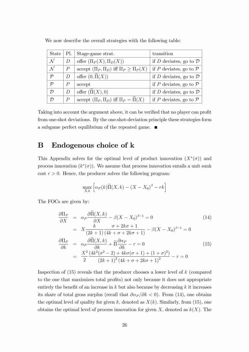
We now describe the overall strategies with the following table:

State Pl. Stage-game strat. transition

N D o¤er (�P (X);�D(X)) if D deviates, go to DN P accept (�P ;�D) i¤ �P � �P (X) if P deviates, go to PP D o¤er (0; e�(X)) if D deviates, go to DP P accept if P deviates, go to PD D o¤er (e�(X); 0) if D deviates, go to DD P accept (�P ;�D) i¤ �P = e�(X) if P deviates, go to P

Taking into account the argument above, it can be veri�ed that no player can pro�t

from one-shot deviations. By the one-shot-deviation principle these strategies form

a subgame perfect equilibrium of the repeated game.

B Endogenous choice of k

This Appendix solves for the optimal level of product innovation (X�(�)) and

process innovation (k�(�)). We assume that process innovation entails a unit sunk

cost r > 0. Hence, the producer solves the following program:

maxX;k

h�P (k)e�(X; k)� (X �X0)

� � rki

The FOCs are given by:

@�P@X

= �P@e�(X; k)@X

� �(X �X0)��1 = 0 (14)

= Xk

(2k + 1)

� + 2k� + 1

(4k + � + 2k� + 1)� �(X �X0)

��1 = 0

@�P@k

= �P@e�(X; k)@k

+ e�@�P@k

� r = 0 (15)

=X2

2

(4k2(�2 � 2) + 4k�(� + 1) + (1 + �)2)(2k + 1)2 (4k + � + 2k� + 1)2

� r = 0

Inspection of (15) reveals that the producer chooses a lower level of k (compared

to the one that maximizes total pro�ts) not only because it does not appropriate

entirely the bene�t of an increase in k but also because by decreasing k it increases

its share of total gross surplus (recall that @�P=@k < 0). From (14), one obtains

the optimal level of quality for given k; denoted as X(k): Similarly, from (15), one

obtains the optimal level of process innovation for given X; denoted as k(X): The

26

solution of the program above is given by the intersection of the two functions.

Note that

dk(X)

dX=

@2�P@k@X

�@2�P@2k

=X 4k2(�2�2)+4k�(�+1)+(1+�)2

(2k+1)2(4k+�+2k�+1)2

�@2�P@2k

:

Since@2�P@2k

< 0 in a neighborhood of the optimal level of k; and since equation (15)

implies 4k2(�2 � 2) + 4k�(� + 1) + (1 + �)2 > 0, it follows that dk(X)dX

> 0.

In turn, we have already proved that

@X(k)

@k=

@2�P@X@k

�@2�P@2X

=X(4k2(�2�2)+4k�(�+1)+(�+1)2)

(2k+1)2(4k+�+2k�+1)2

�(� � 1)(X �X0)��2 � k(2k+1)

�+2k�+1(4k+�+2k�+1)

:

which is positive either if � �p2 or � <

p2 and k su¢ ciently large. However,

since the equilibrium level of k must be such that 4k2(�2�2)+4k�(�+1)+(1+�)2 >0; the intersection between the two functions must be in the increasing part of

X(k).

From (10) we already know that an increase in � shifts upward X(k): From

(15) it follows that an increase in � shifts upward also k(X) :

@k(X; �)

@�=

@2�P@k@�

�@2�P@2k

=4kX2 �+1

(4k+�+2k�+1)3

�@2�P@2k

> 0:

Hence, an increase in � increases both the optimal levels of X and k:

References

[1] Abreu, D. (1986), "On the Theory of In�nitely Repeated Games with Dis-

counting," Econometrica, 56, 383-396.

[2] Battigalli, P. and G. Maggi (2004), "Costly Contracting in a Long-Term Re-

lationships", IGIER w.p. 249.

27

[3] Battigalli, P., C. Fumagalli and M. Polo (2006), "Buyer Power and Quality

Improvement", IGIER w.p. 310.

[4] Bergemann, D. and J. Välimäki (2003), "Dynamic common agency", Journal

of Economic Theory, 111(1), 23-48.

[5] Bernheim, D. and M. Whinston (1986), "Menu Auctions, Resouce Allocation,

and Economic In�uence", Quarterly Journal of Economics, 101, 1-32.

[6] Bonnet C., P. Dubois and M. Simioni (2005), "Two-Part Tari¤s versus Linear

pricing Between Manufacturers and Retailers: Empirical Tests on Di¤erenti-

ated Products Markets", IDEI Working Paper n. 370.

[7] Chae, S. and P. Heidhues (2004), "Buyers�alliances for bargaining power",

Journal of Economics and Management Strategy, 13, 731-754.

[8] Chen Z. (2003), "Dominant retailers and the countervailing-power hypothe-

sis", The RAND Journal of Economics, 34(4), 612-625.

[9] Chen Z. (2006), "Monopoly and Product Diversity: The Role of Retailer

Countervailing Power", mimeo, Carleton University.

[10] Chipty T. and C. Snyder (1999), "The Role of Firm Size in Bilateral Bar-

gaining: A Study of the Cable Television Industry", Review of Economics

and Statistics, 81, 326-340.

[11] Dana, J. (2004), "Buyer groups as strategic commitments", mimeo.

[12] DeGraba P. J. (2005), "Quantity Discounts from Risk Averse Sellers", Work-

ing Paper No. 276, Federal Trade Commission.

[13] Dobson (2005), "Exploiting Buyer Power: Lessons from the British Grocery

Trade", Antitrust Law Journal, 72, 529-562.

[14] Dobson, Paul W. and Waterson, Michael (1997), �Countervailing Power and

Consumer Prices�, Economic Journal, 107, 418-30.

[15] Dobson, Paul W. and Waterson, Michael (1999), "Retailer Power: Recent

Developments and Policy Implications", Economic Policy, 28, 133-164.

[16] Ellison S. and C. Snyder (2002), "Countervailing Power in Wholesale Phar-

maceuticals", Working Paper 01-27, MIT, Cambridge, MA.

28

[17] European Commission (1999), "Buyer Power and its Impact on Competi-

tion in the Food Retail Distribution Sector of the European Union", Report

produced for the European Commission, DG IV, Brussels.

[18] Farber, S. (1981), "Buyer Market Structure and R&D E¤ort: A Simultaneous

Equations Model", The Review of Economics and Statistics, 63(3), 336-345.

[19] FTC (2001), "Report on the Federal Trade CommissionWorkshop on Slotting

Allowances and Other Marketing Practices in the Grocery Industry", Report

by the Federal Trade Commission Sta¤, Washington, D.C.

[20] Galbraith, John Kenneth (1952), American Capitalism: The Concept of

Countervailing Power, Reprint edition. Classics in Economics Series. New

Brunswick, N.J. and London: Transaction, 1993.

[21] Grossman S.J. and O. Hart (1986), "The Costs and Bene�ts of Ownership:

A Theory of vertical and Lateral Integration", Journal of Political Economy,

94(4), 691-719.

[22] Grossman, G. and E. Helpman (1994), "Protection for Sale", American Eco-

nomic Review, 84, 833-850.

[23] Hart O., and J. Moore (1990), "Property Rights and the Nature of the Firm",

Journal of Political Economy, 98(6), 1119-1158.

[24] Horn, H. and A. Wolinsky (1988), "Bilateral Monopolies and Incentives for

Mergers", RAND Journal of Economics, 19, 408-419.

[25] Inderst R. and C. Wey (2005a), "Buyer Power and Supplier Incentives",

mimeo, LSE.

[26] Inderst R. and C. Wey (2005b), "How Strong Buyers Spur Upstream Innova-

tion", mimeo, LSE.

[27] Inderst R. and Wey (2003), "Market Structure, Bargaining, and Technology

Choice in Bilaterally Oligopolistic Industries", RAND Journal of Economics,

34, 1-19.

[28] Inderst R. and G. Sha¤er, "Retail Mergers, Buyer Power, and Product Vari-

ety", forthcoming in the Economic Journal.

[29] Katz, M.L. (1987), "The welfare e¤ects of third degree price discrimination

in intermediate goods markets", American Economic Review, 77, 154-167.

29

[30] Klein B., R. Crawford and A. Alchian (1978), "Vertical Integration, Appro-

priable Rents, and the Competitive Contracting Process", Journal of Law

and Economics, 21, 297-326.

[31] Lustgarten, Steven H. (1975), �The Impact of Buyer Concentration in Man-

ufacturing Industries�Review of Economics and Statistics, 57, 125-32.

[32] Norman H., Ru­ e B. and Snyder C. (2005), "Do Buyer-Size Discounts De-

pend on the Curvature of the Surplus Function? Experimental Tests of Bar-

gaining Models", mimeo.

[33] OECD (1999), "Buying Power of Multiproduct Retailers, Series Roundtables

on Competition Policy", DAFFE/CLP(99)21, Paris.

[34] Peters, J. (2000), "Buyer Market Power and Innovative Activities. Evidence

from the German Automobile Industry", Review of Industrial Organization,

16, 13-38.

[35] Raskovich A. (2003), "Pivotal Buyers and Bargaining Position", Journal of

Industrial Economics, 51, 405-426.

[36] Rey P. (2000), "Retailer Buyer Power and Competition Policy" in Annual

Proceedings of the Fordham Corporate Law Institute (Chapter 27).

[37] Scherer, F.M, and Ross, David (1990), Industrial Market Structure and Eco-

nomic Performance, Boston, Houghton Mi­ in, Third Ed.

[38] Shubik, M. and R. Levitan (1980). Market Structure and Behavior, Cam-

bridge, MA: Harvard University Press.

[39] Snyder, C. M. (1996), �A Dynamic Theory of Countervailing Power�, RAND

Journal of Economics, 27, 747-769.

[40] Snyder, C. M. (2005), "Countervailing Power", manuscript prepared for the

New Palgrave Dictionary.

[41] Tyagi, R. K. (2001), "Why do suppliers charge larger buyers lower prices?",

The Journal of Industrial Economics, 49(1), 45-61.

[42] Vieira-Montez, Joao (2004), "Downstream Concentration and Producer�s Ca-

pacity Choice", mimeo.

30

[43] Villas-Boas, S. (2005), "Vertical Contracts between Manufacturers and Re-

tailers: Inference with Limited Data", CUDARE Working Paper n. 943R2,

University of California, Berkeley.

[44] von Ungern-Sternberg, Thomas (1996), �Countervailing Power Revisited�,

International Journal of Industrial Organization; 14, 507-19.

[45] Williamson, O. (1979), "Transaction-Cost Economics: The Governance of

Contractual Relations", Journal of Law and Economics, 22, 233-61.

31