AD-A241 289 TECHNICAL REPORT CERC-91 -13

EVALUATION OF THE COASTAL FEATURESMAPPING SYSTEM FOR SHORELINE MAPPING

by

Steven G. Underwood, Fred J. Anders

Coastal Engineering Research Center

DEPARTMENT OF THE ARMYWaterways Experiment Station, Corps of Engineers

3909 Halls Ferry Road, Vicksburg, Mississippi 39180-6199

DTIOELECTEf

September 1991

-M WAM Final Report

Approved For Public Release, Distribution is Unlimited

91-12053

Prepared for DEPARTMENT OF THE ARMY

II, ,, "US Arm y Corps of EngineersWashington, DC 20314-1000

9f)

Destroy this report when no longer needed. Do not returnit to the originator.

The findings in this report are not to be construed as an officialDepartment of the Army position unless so designated

by other authorized documents.

The contents of this report are not to be used foradvertising, publication, or promotional purposes.

Citation of trade names does not constitute anofficial endorsement or approval of the use of

such commercial products.

Form ApprovedREPORT DOCUMENTATION PAGE OMB No 0704-0188

A.c n''3 ,I' -iaS'e "e'. es -C' r, el" 3 ed

i52 4302 )d 013 ) d%

1. AGENCY USE ONLY (Leave bianx) 2. REPORT DATE 3. REPORT TYPE AND DATES COVEREDSeptember 1991 Final report

4. TITLE AND SUBTITLE S. FUNDING NUMBERS

Evaluation of the Coastal Features Mapping System for

Shoreline Mapping

6. AUTHOR(S) ,Steven G. Underwood

Fred J. Anders

7. PERFORMING ORGANIZATION NAME(S) AND ADDRESS(ES) 8. PERFORMING ORGANIZATION

USAE Waterwavs Experiment Station, Coastal Engineering REPORT NUMBER

Research Center, 3909 Halls Ferry Road, Vicksburg, Technical Report

MS 39180-6199 CERC-91- 13

9. SPONSORING/ MONITORING AGENCY NAME(S) AND ADDREs:'ES) 10. SPONSORING, MONITORINGAGENCY REPORT NUMBER

US Army Corps of 7ngineersWashington, DC 2t314-1000

11. SUPPLEMENTARY NOTES

Available from National Technical Information Service, 5285 Port Royal Road,

Springfield, VA 22161

12a. DISTRIBUTION AVAILABILITY STATEMENT 12b. DISTRIBUTION CODE

Approved for public release; distribution unlimited

13. ABSTRACT (Maximum 200 words)

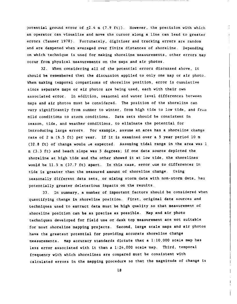
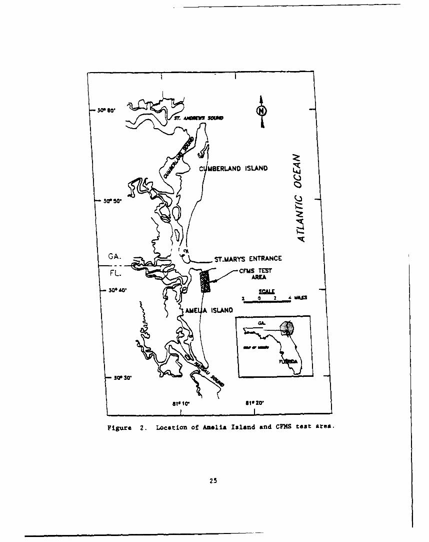
Since many coastal areas are subject to frequent change due to environmen-

tal conditions or commercial devclopment, it is often difficult to fulfill theoptimum requirements for ground control when mapping from aerial photographs.

For this reason, a series of tests were devised to evaluate the accuracy; of the

Coastal Feature Mapping System (CFMS) for tvpical thoreline i.apping applications

encountered by the US Army Corps of Engineers. Major variables tested included

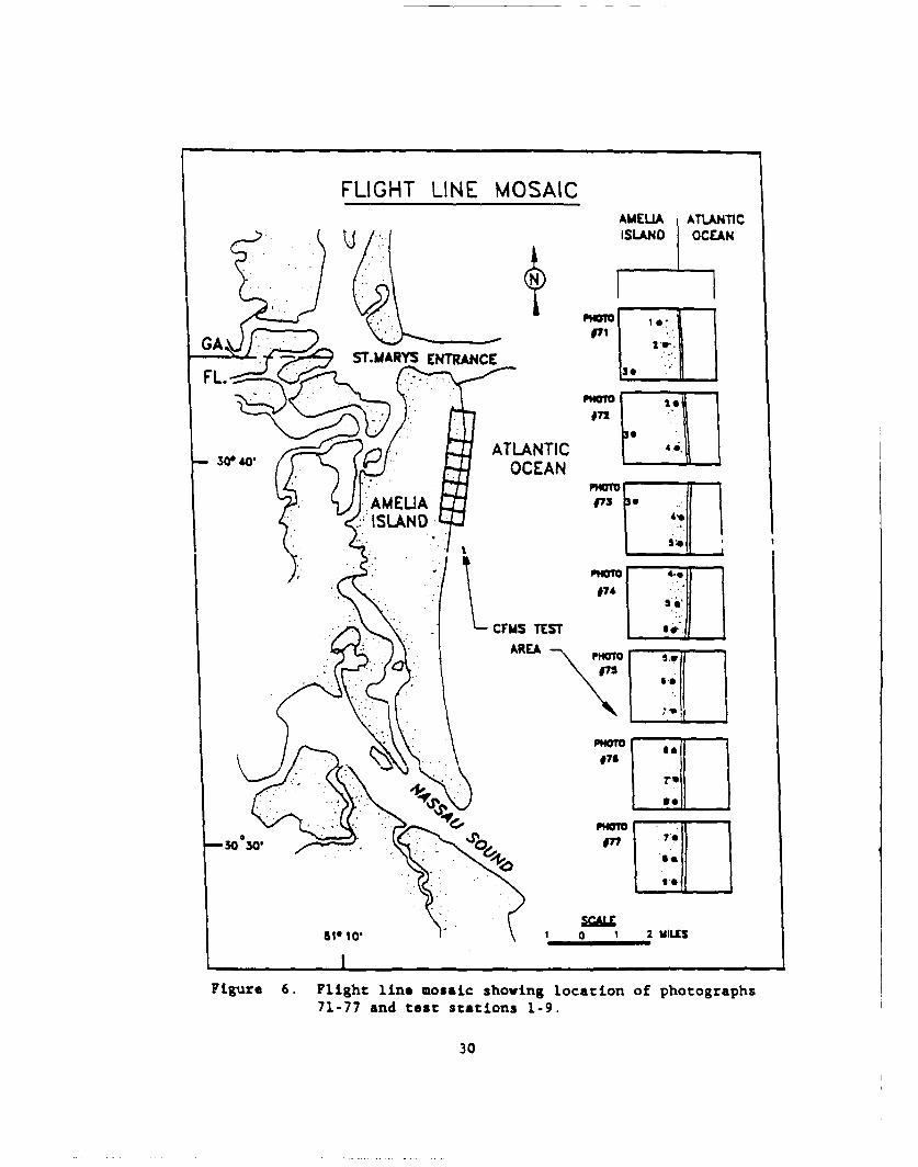
the number of ground control points (GCP's) employed in the solution and their

distribution. Ground control points digitized from 1:24.000 scale US Geologica.

Survey topographic maps were used in various combinations to orient 1:9.600 scile

aerial photographs for coordinate retrieval. It was found that the accuracy; of

X-, Y-coordinates determined from the photographs is governed by the distributio:.nand accuracy of GCP's. Maximum accuracy is obtained when all measured points ar-

within the area bounded by the GCP's. Although at least four GCP's are required

Con-

14. SUBJECT TERMS 15. NUMBER OF PAGESAerial photography 7

Loastal feature mapping system 16. PRICE CODE

Tcpographic maps17. SECURITY CLASSIFICATION 18. SECURITY CLASSIFICATION 19. SECURITY CLASSIFICATION 20. LIMITATION OF ABSTRACT

OF REPORT OF Tni. PAGE OF ABSTRACT

UNCLASSIFIED UNCLASSIFIED I I

"J5N 7540-0 280-5500 Stardard -o'' .98 Re. " R9

2 .'3 2

13. ABSTRACT (Continued).

for Lhe solution, additional points allow possible mistakes to be identifiedand corrected interactively. In all tests, the errors were consistent withthose associi-ed uith 1:24,000 scale base map as defined by National MapAccuracy Standards. The user's guide contained adequata information aboutoverall program operation, but lacked sufficient guidance for first time

users.

eT T TAB El

N

AV81b1it C48

PREFACE

In 1986 the Coastal Structures and Evaluation Branch (CSEB) of the

Engineerirug Development Division (EDD), Coastal Engineering Research Center

(CERC), US Army Engineer Waterways Experiment Station (WES), contracted with

the University of Georgia Research Foundation, Inc., for the Center for Remote

Sensing and Mapping Science to develop personal computer software to assist in

shoreline mapping efforts. Specifically, the coftware was to facilitate use

of air photographs in mapping coastal feature changes. The intent of the CSEB

was to apply this software to current shoreline mapping problems and to future

mapping efforts within CERC and Corps-wide. The software, called Coastal

Features Mapping System (CFMS), was completed in 1989. This report presents

an evaluation of CFMS for use in Corps shoreline mapping applications.

This report was prepared by Messrs. SLeven G. Underwood and Fred J.

Anders of the Coastal Geology Unit (CGU), CSEB, CERC. Funding for software

development was provided through the Evaluation of Navigation and Shore

Protection Structures Program, and funding for this report was provided by the

Barrier Island Sedimentation Studies Work Unit 31665. This study was spon-

sored by Headquarters, US Army Corps of Engineers (HQUSACE). Program manager

is Dr. C. Linwood Vincent, and HQUSACE Technical Monitors are Messrs. John H.

Lockhart, Jr.; John G. Housley; James E. Crews: and Robert H. Campbell.

The work was conducted under the general supervision of Ms. Joan Pope,

Chief, CSEB; Mr. Thomas Richardson, Chief, EDD, CERC; Mr. Charles C. Calhoun,

Jr., Assistant Chief, CERC; and Dr. James R. Houston, Chief, CERC. Other CERC

personnel participating in the report preparation included: Ms. Karen

Pitchford, Atlantic Research Corporation, who provided technical assistance

and helped with experimental design criteria for CFMS; Ms. Lynn Bessonette,

CERC contract student, who contributed AutoCAD drawings for this report;

Mr. Mark Hansen and Dr. Mark R. Byrnes, both formerly with CERC; Dr. Roy Welch

and Mr. Tommy Jordan from the University of Georgia's Center for Remote

Sensing and Mapping Science, who provided technical reviews; and Ms. Laurel

Gorman, EDD, CERC, who assisted with the Kings Bay background.

Commander and Director of WES during publication of this report was

COL Larry B. Fulton, EN. Technical Director was Dr. Robert W. Whalin.

1

CONTENTS?Age

PREFACE ......................................... 1I

LIST OF FIGURES....................... ......................... 3

PART I: INTRODUCTION....................................... 4

Shoreline Change Mapping................................. 4The Coastal Feature Mapping System....................... 6

PART II: AN INTRODUCTION TO MEASURING; qHORELINE CHANGE ... 7

Problems and Sources of Error............................ 7Shoreline Mapping and Analysis Techniques ................ 19

PART III: AN EVALUATION OF CFMS.............................. 24

Ground Control Point (GCP) Distribution .................. 26The Bridging Concept ...... I.............................. 33Bridging (Control on Both Ends)........................ jBridging (Control on One End)............................ 34

PART IV: SUMMARY AND CONCLbL2'NS......................... 38

REFERENCES..................................................... 40

APPENDIX A: SHORELINE CHANGE ALONG A DEVELOPED COAST:NORTH AMELIA ISLAND, FLORIDA..................... Al

2

LIST OF FIGURES

Figure Page

I Shows relationship between a tilted and exactlyvertical photograph ..................................... 15

2 Location of Amelia Island and CFMS test area ......... 25

3 Test station diagram for variable number GCP'sand variable GCP distribution .......................... 27

4 Position difference values for 10 test stationswith Large no. GCP's (9) vs Small no. GCP's (4) ...... 28

5 Position difference values for 10 test stationswith Well distributed GCP's vs Poorly distributed .... 28

6 Flight line mosaic showing location of photographs71-77 and test stations 1-9 ............................. 30

7 7 photcgraph GCP test showing average positiondifferences when comparing CFMS location to basemap location ............................................ 32

8 Position differences-Bridging 5 photographs.... 35

9 Position differences-Bridging 4 photographs .......... 35

10 Position differences-Bridging 3 photographs .......... 35

11 Position differences for test stations 2, 3, 4- GCP's one end only .................................... 36

12 Position differences for test stations 5, 6, 7, 8- GCP's one end only .................................... 36

13 Updated 1988 Amelia Island shoreline, and AbsoluteShoreline Movement ...................................... A4

3

AN EVALUATION OF THE COASTAL FEATURES MAPPING SYSTEM

FOR

SHORELINE MAPPING

PART I: INTRODUCTION

Shoreline Change Maping

I. Knowledge of past and present shoreline change rates is essential

for most planning, geomorphic, and engineering projects in the coastal zone.

Quantitative historical changes are used to develop qpdiment budgets, monitor

engineering modifications to the shoreline, plan engineering projects, examine

geomorphic variations in the coastal zone, examine the role of natural

processes in modifying shorelines, establish set back lines, and predict

future shoreline changes. This information can be obtained from either

continucus field surveys or from current and historic maps and vertical aeripl

photogiaphs. The latter does not require extensive field time nor expensive

equipment to collect data and, therefore, it is often the most economical

means of measuring shoreline change. Scientists, engineers, and planners have

recognized the usefulness of mapping shoreline position to delimit areas of

erosion and accretion. Historical maps dating back to the middle to late

1800's and near-vertical aerial photographs (referred to throughout the

remainder of the text as air photos) beginning in the 1930's are available for

most of the U.S. shoreline, providing a length of record which is not usually

available with field surveys. Therefore, historical change in shoreline

position based on maps and air photos is a useful tool to examine past coastal

changes which have resulted from incident processes and to project future

changes in shoreline response.

2. Technically, the shoreline is the line of intersection defined by

land, sea, and air, and it is in a constant state of change, making mapping

difficult. Shoreline position and configuration at any point in time and

space is a function of five primary factors: pre-existing geology, sediment

supply, process energy, sea level rise, and human intervention. Interaction

among these factors determines shoreline location at any instant in time.

4

Developing accurate maps is a difficult task anywhere, but mapping the

shoreline presents additional problems because of its constantly changing

position. Historical analysis of shoreline changes is therefore hindered by

the long periods of time between successive maps. Air photos can supplement

maps by recording the shoreline at a given time and they can be collected as

frequently as funding permits. They do, however, present several potential

problems.

3. Although the difficulties in preparing a shoreline map are numerous.

comparing shoreline changes on successive maps and air photos is even more

challenging. Shoreline maps must be evaluated for accuracy, corrected to

reflect a common tidal datum, and brought to a common scale before data from

successive maps can be compared. Electronic digitizers and computers with a

variety of software have greatly facilitated the use of maps for comparing

shoreline position. However, initial map accuracy must still be evaluated to

assess the signifirance of measured changes. Air photos must be evaluated for

a variety of distortions inherent in the photographic process which must be

rectified if they are to be treated as maps Several techniques have been

developed to correct distorLions in air photos so that they may be used to

supplement map data. These techniques, of which the Coastal Features Mapping

System (CFMS) is one, will be discussed in this report. To date, none of the

available techniques have successfully removed all photographic distortion at

a reasonable cost.

4. The primary purpose of this report is to evaluate the use of CFMS

for typical shoreline mapping applications encountered by the Corps of

Engineers. These applications generally involve the use of both maps and air

photos. CFMS allows the user to digitize information from both data sources

and draw map oveflays of corrected shorelines. The accuracy and ease with

which this is accomplished are evaluated. In addition, a summary is provided

of the various techniques developed to quantify historical shoreline change,

typical problem areas and sources of error, and how CFMS contributes to

shoreline change evaluation.

The Coastal Features Mapping System

5. The CFMS is a PC-based program that numerically removes photographic

distortions common to air photos of the coastline. The general technique

employed involves selection of ground contrn! points (GCP's) for which exact

position is known in a cartesian coordinate system. Location of these points

could be determined from field surveys or from a base map. The points are

identified on air photos, and their position is corrected with reference to

the known location using a l .st squares fit. The correction applied to

control points is then used to adjust shoreline points being mapped. The end

result is a series of shoreline points that are adjustzd to compensate for

photographic distortion and a composite map of all shorelines (generated from

original maps and air photos) at a common scale. This technique offers the

advantages of ease of use and speed of operation and it is a fairly

inexpensive correction technique. However, it does not completely remove a!.

distortion and is particularly limited in areas of high relief.

6. One additional benefit of CFMS is its ,bilitv to extend control into

areas wh' re -one exists. Typically, the exact coordinates of stable ground

control points, upon which the correction factor is baspA. are difficult to

locate. This is espcalv true in many unpopulated coastal areas. CFMS uses

a bridging techn roe . ;xterc control between aerial photos containing GCP's

to up to 2 !itermediate pho;os that have few stable points or none at all.

6

PART II: AN INTRODUCTION TO MEASURING SHORELINE CHANGE

7 A variety of techniques have been developed to extract shoreline

change data from maps and air photos. These techniques range from purely

mechanical measurement of shoreline position through automated systems. Cost

generally increases with automation, but so does ease =f data collection and

accuracy with which shoreline change is known. A discussion of the various

techniques used is prefaced by a discussion of typical problems associated

with using maps and air photos for determining shoreline change. These

problems have important bearing on data accuracy and therefore should be given

careful consideration before starting an analysis.

Problem and Sources of Error

Recent Maps

8. The accuracy of shoreline change measurements depends on map scale

The smallest field distance measurable on a 1:20,000 scale map is 4 m (13 ft,

Tanner 1978). Shoreline measurements can only be as accurate as the original

maps themselves. Accuracy depends on the standards to which each original map

was made and on changes which may have occurred to a map since its original

publication. Since 1941 strict standards of accuracy have been defined for

published maps. For examining shoreline position, the two most commonly

available maps are US Geological Survey (USGS) Quadrangles and National Ocean

Service (NOS) Charts. Both of these map types meet or exceed national map

accuracy standards. United States National Map Accuracy Standards (Appendix

6, Ellis 1978) state:

"For maps on publication scales larger than 1:20.000, not more

than 10 percent of the points tested shall be in error by more

than 1/30 inch [0.846 mm] measured on the publication scale; for

maps on publication scales of 1:20,000 or smaller, 1/50 inch

[0,508 mm]. These limits of accuracy shall apply in all cases to

positions of well-defined points only. Well-defined points are

those that are easily visible or recoverable on the ground, such

as the following: monuments or markers, such as bench marks,

property boundary monuments; intersections of roads, railroads,

etc.; corners of large buildings or structures (or center points

7

of small buildings); etc."

9. USGS topographic maps at a scale of 1:24,000 are the most commonly

used maps for determining shoreline change. Applying the accuracy standard to

these maps, maximum allowable error for 90% of the stable points is 12 ra (40

ft). The accuracy with which any non-stable shoreline point is located could

be less. NOS produces a variety of nautical charts at a variety of scales.

For determining shoreline change the most commonly used chart is the

Topographic (T) Sheet, which is the basic chart from which nautical and

aeronautical charts are constructed. T sheets are generally produced at a

scale of 1:10,000, although 1:5,000 and 1:20,000 charts have been made. At

the 1:10,000 scale, national standards allow up to 8.5 m (28 ft) of error fcr

a stable point. Other non-stable points are located with less accuracy,

however, features critical to safe marine navigation are mapped to standards

stricter than national standards (Ellis, 1978). The shoreline is mapped to

within 0.5 mm (.02 inch, at map scale) of true position, which at 1:10,000

scale is about 4.9 m (16 ft) on the ground. Fixed aids to navigation and

objects to be charted as landmarks must be located to withi, 3 m (10 ft) at

this scale. In a shoreline mapping project using NOS charts, 36 random

features such as road intersections and shoreline features, including points

of marsh, were scaled from maps compiled from air photos. These features were

located by field traverse ariA iere compared with the geodetic coordinate

values. The check revealed a maximum e-ror of +3.0 m (10 ft, Everts, Battlev,

and Gibson 1983).

10. For accurate shoreline change measurement, NOS T sheets are the

preferred data source. However, in cases were T sheets are not available or

where a rapid and less accurate estimate of shoreline change is sufficient,

such as areas where shoreline change is very large, USGS topographic maps can

be used with confidence. Other maps depicting the shoreline may also be

available in US Army Corps of Engineers offices and State and Local government

offices. Usefulness of these maps for quantifying shoreline change depends on

their accuracy standards and scale.

11. As previously mentioned, map accuracy also depends on what changes

the map has undergone since production. Most important are changes in

horizontal and vertical datums and physical changes resulting from shrinking

8

or stretching of the medium on which the map is printed. Horizontal and

vertical datums were standardized in 1927 and 1929 respectively. Maps

completed prior to this time require correction to the coordinate system to

conform with new datums. In 1983, the horizontal datum (North American Datum

- NAD) was readjusted using a newly defined ellipsoid referenced to the

earth's center of mass. Readjustment resulted in a change in State Plane and

Universal Transverse Mercator (UTM) coordinate systems with respect to

geographic coordinates (latitude and longitude) and each other. In the 48

lower states differences range from 0 to 110 m (360 ft) and up to 200 m (660

ft) in Alaska and 400 m (1310 ft) in Hawaii. As of this writing, nautical

maps are being published with the new horizontal datum, but to date USGS maps

have not been regularly published with the new datum. Eventually all

published charts and maps will referance the 1983 NAD. Shrink and stretch is

a problem which can occur over very short time periods with paper maps.

Knowle- and Gorman (in press) estimate potential changes between 0.03 and 0.25

mm (0.001 and 0.01 in), which at 1:10,000 scale is +0.3 - 2.5 m (1 - 8 ft) of

ground distance. This problem can be avoided by using maps printed on a

stable base material such as mylar.

12. One additional factor to consider when measuring shoreline change

from maps is which shoreline has been mapped. Mean-high-water (MHW) and mean-

low-water (MLW) are the two most commonly mapped shorelines. On gently

sloping beaches with a moderate tidal range, the difference can be significant

and corrections to a common position must be made when using maps with

different shorelines. USGS topographic maps generally depict the shoreline at

the MHW position, although newer maps may also have the MLW line plotted. NOS

T sheets often have the MHW line marked as bold and the MLW shoreline is

dashed.

Historical Maps

13. The question of accuracy becomes even more important when dealing

with maps made prior to the 1941 National Map Accuracy Standards. Old maps

are extremely useful for determining the long term history of shoreline

change, but their accuracy must be carefully evaluated. Earliest NOS T sheets

(US Coast and Geodetic Survey) date back to the 1830's and USGS topographic

maps date back to formation of the USGS in 1879. Accuracy of regional maps

9

developed prior to these dates are highly suspect. Local maps may be accurate

enough for quantitative shoreline change measurement, but regional maps can,

at best, be used only for qualitative assessment of shoreline movement.

14. Originally, T sheets were made from actual topographic field

surveys (modern maps are made from air photos). Shalowitz (1964) notes that

during these surveys, mapping the high-water shoreline was the most important

consideration. However, accuracy of early surveys can still be questioned

since the only standards were those maintained by individual field party

bosses. In 1840 the first superintendent of the US Coast and Geodetic Survey,

Ferdinand Hassler, issued instructions to carefully survey the high-water

shoreline (Everts, Battley, and Gibson 1983). While surveying the high-water

line, the low-water line was to be mapped by taking offsets, unless the two

lines were far apart, which would require separate surveys.

15. More specific instructions on topographic mapping of the shoreline

were written in 1889 by Wainwright in the Plane Table Manual. Shalowitz

(196t) interprets instructions to field parties as follows:

"The mean high-water line along a coast is the intersection of the

plane of mean high water with the shore. This line, particularLy

along gently sloping beaches, can only be determined with

precision by running spirit levels along the coast. Obviously,

for charting purposes, such precise methods would not be

justified, hence, the line is determined more from the physical

appearance of the beach. What the topographer actually delineated

are the markings left on the beach by the last preceding high

water, barring the drift cast up by storm tides."

"In addition to the above, the topographer, who is an expert in

his field, familiarizes himself with the tide in the area, and

notes the characteristics of the beach ... and the tufts of grass

or other vegetation likely along the high-water line."

16. In summary, Shalowitz (1964) notes it was the intention of the

surveyors to determine the line of MHW for delineation on maps, and therefore,

despite the lack of standards, this task was not treated lightly by individual

survey parties.

17. Just how precisely the MHW line was located on these early surveys

10

was also addressed by Shalowitz (1964). He notes,

"The accuracy of the surveyed line here considered is that

resulting from the methods used in locating the line at the time

of survey. It is difficult to make any absolute estimates as to

the accuracy of the early topographic surveys of the Bureau. In

general, the officers who executed these surveys used extreme care

in their work. The accuracy was of course limited by the amount

of control that was available in the area."

"With the methods used, and assuming the normal control, it was

possible to measure distances with an accuracy of 1 meter (Annual

Report, US Coast and Geodetic Survey 192, 1880) while the position

of the planetable could be determined within 2 or 3 meters of its

true position. To this must be added the error due to the

identification of the actual mean high water line on the ground,

which may approximate 3 to 4 meters. It may, therefore, be

assumed that the accuracy of location of the high-water line on

the early surveys is within a maximum error of 10 meters and may

possibly uc much more accurate than this. This is the accuracy of

the actual rodded points along the shore and does not include

errors resulting from sketching between points. The latter may,

in some cases, amount to as much as 10 meters, particularly where

small indentations are not visible to the topographer at the

planetable."

18. Measurement accuracy of the MHW shoreline on early surveys is thus

dependent on a variety of factors, not the least of which was the ratio of

actual rodded points to sketched data used by an individual surveyor. The

more sketching used, the lower the overall accuracy. However, by means of

triangulation control, a constant check was applied to the overall accuracy of

the work so that no large errors were allowed to accumulate.

19. Based on this knowledge of topographic and cartographic procedures

used in the past, use of old T sheets and quadrangles for quantifying

shoreline change seems reasonable provided potential errors are recoanized and

stated. It must be remembered that rates of shoreline change derived from

analysis of maps and air photos cannot be considered absolute. Neither the

11

accuracy of historical maps or modern maps is sufficient to give more than a

good estimate of trends in shoreline erosion or accretion. Accuracy of

original data sources are just not sufficient to discriminate between

shorelines measured at close intervals of time or with slowly changing

shorelines.

20. For example, assume a shoreline is eroding at 1 m/yr. After 8

years the shoreline would have moved landward 8 m (26 ft). If we wanted to

determine the rate of retreat of that shoreline using two maps we would have

to consider the error present in each map. Accuracy standards for modern NOS

T sheets allows an error of up to 4.9 m (16 ft) in locating the shoreline.

Summing the error for each map gives us a error band of 9.8 m (32 ft,

additional sources of error could be added to this). The 8 m (26 ft) of

actual erosion falls within this error band and thus the observed map

differences cannot be considered significant. If we examine the same

shoreline on two maps 100 years apart, 100 m (328 ft) of shoreline change is

significant in comparison to 9.8 m (32 ft) of error. In another instance, if

our rate of shoreline change were nnlv 0.1 m/yr (as is the case with many bay

shorelines) over 50 years we would have only 5 m (16.5 ft) of change, which

again falls within the 9.8 m (32 ft) band of error.

21. In summary, to quantify historical shoreline change rates with some

degree of confidence requires shoreline change to be large or the time

interval between maps or air photo sets to be large. It is also useful to

have intermediate data sources between the first and last dates to serve as a

check on overall rate of shoreline change.

Near-Vertical Aerial Photographs

22. Generally, only very long term trends can be determined from NOS T

sheets or USGS topographic maps since they are produced at infrequent

intervals. This may preclude a detailed understanding of short term physical

processes and morphological responses. Additionally, many details of the

subaerial beach are not represented on these maps, which can make location of

control points for shoreline analysis difficult and eliminates the use of some

scientifically significant information. Air photos can be used to supplement

shoreline change measurements by providing data on a shorter time interval and

with level of detail unavailable with maps.

12

23. The use of air ptos as a tool for measurement of shoreline change

began in the late 1960's (Moffitt 1969, Langfelder, Stafford, Amein 1970,

Stafford and Langfelder 1971). Prior to this, air photos had been used to

qualitatively assess changes in coastal landforms. Vertical black and white

air photos date back to the late 1920's, but reasonably good quality stereo

air photos were not available until the late 1930's. In recent decades, air

photo missions have been flown by numero- federal, state, and private

organizations, making temporally frequent near-vertical aerial photography

available at a reasonable cost for most US shorelines.

24. For locating coastal features in the field, good quality air photos

can be used directly with less concern for accuracy. However, air photos

cannot be treated as maps for quantification of shoreline change. A variety

of distortions are inherent in air photos which must be eliminated or

minimized to reduce measurement errors to an acceptable level. Almost all

features on a air photo, except those near the center of the photo, occupy

positions other than their true relative map positions. Photographic

distortions due to camera optics is a problem in older air photns, but is not

a big consideration for mapping camera's manufactured since sne mid-1940's.

25. Relief or elevation displacement, due to large vertical changes in

topography can also be a source of error. At the moment of exposure,

features further from the lens, such as valleys, appear at a smaller scale on

the air photo than features that are closer to the lens, such as mountains.

The displacement of points on a air photo as a result of terrain relief, is

radial from the nadir point (the point vertically below the camera) (Figure

1). For truly vertical aerial photographs the nadir point and principal point

(center of the photo) coincide. Displacement of an image due to relief

displacement (d.) can be calculated as:

d. - rh/H

where r is the distance on the photograph from the center to the image of

the top of the object, h is the ground elevation of the object, and H is

the flight altitude of the camera relative to the same datum as h (Wong,

1980). Most coastal features have low relief so that radial distortion due to

elevation differences is not a serious problem. However, measurement of

shorelines backed by bluffs and cliffs with vertical relief of several meters

13

could result in errors. The position of stable points on top of bluffs

relative to shorelines at the base could be significantly displaced. For

example, if a control point located on top of a cliff 10 m (32 ft) above mean

sea level (MSL), is 7 cm (2.8 in? from the center of the air photo, and the

altitude of the airplane was 1463 m (4800 ft) above msl (with a 152.4 mm (6

in) focal length lens, this would correspond to a 1:9600 scale air photo) its

geographic position would be displaced 0.48 mm (.02 in? on the air photo,

which corresponds to 4.6 m (15 ft) of displacement on the ground. Depending

on the relative positions of land and sea, this could be falsely interpreted

as shoreline erosion or accretion.

26. Scale variations across the photo due to tilt can result when the

airplane attitude is not exactly parallel to the mean plane of the earth's

surface at the instant of exposure. About half of the near-vertical aerial

photographs taken for domestic mapping purposes are tilted less than 2

degrees, and few are tilted more than 3 degrees (Wong 1980). Up to 7 degrees

of tilt can occur in air photos taken for non-mapping purposes. Many coastal

scientists have ignored the problem of point displacement due to tilt in

imagery. 6ume correction for tilt distortion must be made on almost every air

photo prior to mapping. The relationship between a tilted and exactly

vertical air photo is illustrated in Figure 1. On the upper side of the air

photo, scale is larger and images appear to be displaced radially toward the

isocenter, and radially away from the isocenter on the lower (smaller scale)

side of the air photo.

14

-NGLE OF TILT

4------ - - - - -

-DISPLACEMENT

NGLE OF TILTDUTOIL

Figure 1. Shovs relationship betveen a tilted and exactly

vertical photograph.

15

27. Displacement of a point on a air photo due to tilt (Dt) from its

actual ground position can be calculated using the following relationship

(after Wolf 1983),

D, - [r 2(sin t)(cos 2 P)]/[f - Ir sin t)(cos P)J,

where r is the distance from the point to the isocenter, f is the focal length

of the lens, t is the angle of tilt of the photograph, and P is the angle

measured clockwise from the principal line to radial line between the

isocenter and the point (within the plane of the photograph). As is apparent

from this equation, the amount of displacement increases with distance from

the isocenter and with increasing tilt. Using air photos with minimal tilt

and working only at the center of the air photo minimizes point displacement.

However, for a tilt angle of only 1 degree, a point 10.0 cm (3.9 in) from the

isocenter and 40 degrees from the principal line on a 1:20,000 air photo,

would have an error of 6.5 m (21.3 ft) in its true ground location. An air

photo with 3 degrees of tilt would yield an error of 19.7 m (64.6 ft) in its

ground location, which means a shoreline could be displaced by this amount

from its actual position. Clearly, unless one is working only in the center

of a air photo, some correction for tilt distortion must be made.

28. One other possible source of measurement error in air photos is

changing scale along the photographic flightline. Especially in light

aircraft, altitude of the airplane may change slightly as it follows a flight

line. The result is that scale may vary slightly from one air photo to the

next. Exact scale of each air photo should be determined so that appropriate

factors are used when digitizing or scaling data from a air photo.

Photographic scale (S) can be calculated by,

S - l/(H/f)

where f is the focal length of the camera lens and H is the height of the

camera above the mean elevation of the terrain (in similar units) (Wong 1980).

The result is a representative fraction corresponding to map scale. Scale may

also be determined if the distance between two points or size ot an object is

known in the field or on an accompanying map.

16

29. To illustrate the effect of scale variation the following example

is presented. At the start of an air photo mission the elevation of the plane

is 3048 m (10,000 ft) and a 152.4 mm (6 in) focal length lens is used, for a

scale of 1:20,000. However, if the elevation of the aircraft changes by 7.6 m

(25 ft) during the mission (15 m (50 ft) is not uncommon in small light

planes), at the moment of exposure, the scale of that air photo will be

1:19950. If we use this air photo and measure the distance between a stable

point and a shoreline position as 7 cm (2.8 in) apart, assuming a scale of

1:20,000 we would calculate ground distance between the !r~-blc point nnd the

shoreline to be 1400 m (4593.2 ft). However, if the scale is actually

1:19950, the distance between the points is 1396.5 m (4581.7 ft), which would

effect a 3.5 m (11.5 ft) error in location of the shoreline.

Other Sources of Error

30. In addition to errors inherent in maps and air photos used for data

collection, errors in shoreline positions can be introduced from

internretation and physical measurement of the shoreline and control points.

un inaps the shoreline is delineated; however, on air photos the shoreline must

first be annotated by a trained interpreter. The high water line on a beach,

generally recognized by a change from dark to light tones, is usually mapped

as the shoreline (Stafford and Langfelder 1971). Correct interpretation of

this line, and careful annotation are required to avoid large errors. Even

width of the annotated line may introduce an error in precision of several

meters at gr-und scale. Most techniques require location of stable control

points on maps and air photos. Road intersections and buildings are logical

control points, but scale of the air photo or the undeveloped character of a

coastline often eliminates these features from the photo scene. In these

cases, other, less precise control points can be used (e.g. a meander bend in

a tidal creek which appears to have remained stable over the time span of the

shoreline change study), or control must be bridged from adjacent air photos.

Unless high-precision stereoscopic plotters are used for bridging, both of

these alternatives reduce accuracy of the shoreline measurement.

31. Modern digitizers are accurate, however, some small amount of error

can still be introduced (e.g. a standard Calcomp 9100 model digitizing tablet

has a accuracy of ±0.254 mm (0.010 in), which at a scale of 1:9600 is a

17

potential ground error of ±2.4 m (7.9 ft)). However, the precision with which

an operator can visualize and move the cursor along a line can lead to greater

errors (Tanner 1978). Fortunately, digitizer and tracking errors are random

and are dampened when averaged over finite distances of shoreline. Depending

on which technique is used for making shoreline measurements, other errors may

occur from physical measurements on the maps and air photos.

32. When considering all of the potential errors discussed above, it

should be remembered that the discussion applied to only one map or air photo.

When making temporal comparisons of shoreline position, error is cumulative

since separate maps or air photos are being used, each with their own

associated error. In addition, seasonal and water level differences between

maps and air photos must be considered. The position of the shoreline can

vary significantly from summer to winter, from high tide to low tide, and frum

mild conditions to storm conditions. Data sets should be consistent in

season, tide, and weather conditions, to eliminate the potential for

introducing large errors. For example, assume an area has a shoreline change

rate of 2 m (6.5 ft) per year. If it is examined over a 5 year period 10 m

(32.8 ft) of change woula ue expected. Assuming tidal range in the area was I

m (3.3 ft) and beach slope was 5 degrees; if one data source depicted the

shoreline at high tide and the other showed it at low tide, the shorelines

would be 11.5 m (37.7 ft) apart. In this case, error uue to differences in

tide is greater than the measured amount of shoreline change. Using

seasonally different data sets, or mixing storm data with non-storm data, has

potentially greater deleterious impacts on the results.

33. In summary, a number of important factors should be considered when

quantifying change in shoreline position. First, original data sources and

techniques used to extract data must be high quality so that measurement of

shoreline position can be as precise as possible. Map and air photo

techniques developed for field use or desk top measurement are not suitable

for most shoreline mapping projects. Second, large scale maps and air photos

have the greatest potential for providing accurate shoreline change

measurements. Map accuracy standards dictate that a 1:10,000 scale map has

less error associated with it than a 1:24,000 scale map. Third, temporal

frequency with which shorelines are compared must be consistent with

calculated errors in the mapping procedure so that the magnitude of change is

i8

greater than potential errors. As discussed above, larger temporal spacing

between data sets improves reliability of shoreline change measurements.

Shoreline Mapping and Analysis Techniques

34. The use of maps and air photos to determine rates of shoreline

change generally requires two separate tasks: compilation of a composite

shoreline change map, and analysis of the composite map to determine specific

rates of change along the shoreline. A variety of techniques have been

presented in the literature for compiling shoieline change idaps, but many of

these techniques still require hand measurement of the composite map to

generate data for determining rates of change. Other techniques have been

developed to determine shoreline change rates directly from original data

sources without developing a shoreline change map. More recently, automated

systems have become available which will allow compilation of shoreline change

maps and rapid calculation of shoreline change rates.

35. Production of shoreline change information using only maps and

charts is a straight forward process (potentiai crrors, such as datum changes,

must be corrected). It simply involves enlarging or reducing all maps and

charts to a common scale and overlaying them. Once overlaid, a composite map

can be drawn and changes in shoreline position can be measured. Enlargement

or reduction and overlaying can be accomplished in a variety of ways.

Numerous instruments, such as a Map-o-Graph, Zoom Transfer Scope, and several

types of projecting light tables can make this an easy manual task.

Alternatively, map data can be digitized, and with a variety of software

packages can be plotted at a common scale. Automation of the processes is a

good choice if many shorelines are to be mapped. Once a composite shoreline

map is completed, determination of rates of change along the coast can

proceed.

36. The use of air photos, with or without maps, for determining rates

of shoreline change is significantly more involved than just using maps. This

is because of relief and tilt distortions inherent with air photos, as well as

scale variations from aircraft height. Stafford (1971), and Stafford and

Langfelder (1971), present the point measurement technique for determining

shoreline change rates from air photos. This technique uses only the center

19

of air photos, which minimizes tilt distortion (relief distortion is not a

problem for most coastal areas unless cliffs border the coastline). Scale

variations must always be corrected. Stable points are selected along the

coast, and from these measurements, adjustments are made to the shoreline on

each air photo and map relative to a cartesian coordinate system. From these

data, rates of shoreline change can be calculated in the vicinity of each

control point. This technique does not produce a composite shoreline change

map and is limited in density of measurements to the number of control points

available.

37. Any technique which attempts to use air photos to produce an

accurate composite shoreline change map must rectify the air photo or data

derived from the air photo for tilt and relief distortion and scale

variations. In recent years a variety of manual techniques have been used.

Most photogrammetric companies and government agencies can produce rectified

air photos by removing tilt and scale variations on large stereoscopic

plotters. These machines essentially take the air photo and put it back inLo

its tilted position, then project the scene downward at the proper scale. The

projected image has all tilt and scale variations removed, producing

rectified vertical aerial photograph that can be treated as a regular map.

Smaller instruments, such as the Vertical sketchmaster work on the same basic

principle to remove tilt, but are not as precise in their operation.

Projecting instruments, such as light tables and the Map-O-Graph can remove

scale variations between air photos, but cannot correct for tilt distortion.

The Zoom Transfer Scope likewise can correct for scale variations, and

partially correct for tilt. It can shrink or stretch an image in one

direction, however, since tilt causes half the air photo to have a larger

scale and half vo have a smaller scale, shrinking or stretching in one

direction is not sufficient to remove all tilt. Aligning carefully selected

control points, and working in small areas of the air photo at a time has

produced best results (Anders and Leatherman, 1982).

38. Over the past decade, a variety of automated techniques have been

developed for producing composite shoreline maps from air photos. Several

personal computer software packages are available which allow a small mapping

laboratory to produce comav1 iite shoreline maps from original map and air photo

data sources. In addition, a few coastal scienLists have developed their own

20

automated techniques (Leatherman 1983). For air photos, most of these

techniques use a least squares adjustment to rectify the data to a non-tilted

condition. This procedure involves digitizing control point information on a

air photo and comparing the location of each point to its known location in a

geographical coordinate system. The least squares procedure then develops a

correction factor to adjust control points to their "proper" position. In so

doing, the correction is not specific to tilt or scale variation, but simply

corrects for all inherent errors simultaneously. The resulting correction is

a "best fit" position for all control points. Using more control points

generally improves the fit by distributing the error between more points.

Once a correction factor is calculated, it is applied to all shoreline data

points digitized from the air photo. Corrected data can then be added to a

cumposite shoreline map. 1h is same general technique is employed in the CFMS

discussed below.

39. After development of a composite shoreline change map, data must

be extracted to determine rates of shoreline change along the coast. Recent

studies by Byrnes et al. (1989) and Anders. Reed, Meisburger (1990) have

determined shorel.i,. change rates at 50 meter intervals along the coast, but

if needed, smaller intervals could be used. Values for each interval can be

summarized to determine shoreline change rates for any length of coast. Data

collection for determination of change rates can either be accomplished

manually or using an automated technique. The manual process involves

establishing transects perpendicular to the composite coastline at the desired

along-the-coast interval and measuring distances between shorelines along each

transect. The amount of change is divided by the time interval between

shorelines to determine rate of change. This should be accompanied by

temporal standard deviation of the change rate for each transect. Spatial

standard deviation is required if shoreline change data is summarized for an

area. The manual technique is suitable if the along-the-coast iaterval is

large so that a limited number of data points are collected.

40. For projects covering large areas with a high density of shoreline

change measurements, automated techniques can save significant amounts of time

and money. The basic procedure is similar to the manual technique. Transects

are established perpendicular to an arbitrary baseline that is parallel to the

composite shoreline, and the intersection of these transects with each

21

shoreline represents a data point. Baseline length was based on general

shoreline orientation and natural breaks in shoreline continuity. Anders,

Reed, and Meisburger (1990) used a cartesian coordinate system for each

baseline with the x-axis directed alongshore and the y-axis directed offshcre.

The digitizer x-increment matched the composite map scale to generate

shoreline change data at approximately a 50 m (165 ft) along-the-coast

interval. Byrnes et al. (1989) used a similar technique, however, high-water

shoreline positions were digitized with reference to a geographical graticule

Digital data were converted to state plane coordinates and referenced to a

common baseline parallel to the shoreline trend. Cubic spline interpolation

was used to compare temporal data at common alongshore positions.

41. An improvement to this technique is currently being developed

(Knowles and Gorman, in press). In a iterative process for each shoreline,

the system, known as COAST (COmputer Analysis of Shoreline Trends) creates a

best fit line through a series of digitized shoreline points (the number of

points is user specified) using a linear regression. These small straight

line segments for each shoreline are averaged to create a mean shoreline

position. COAST establishes transects pe~pendicular to the mean shoreline at

an along-the-coast interval specified by the user, and searches the digitized

data to determine the intersection of each transect with each shoreline. Data

along each transect are then used to calculate a rate of shoreline change.

42. Shoreline change information should include average shoreline

change rate, standard deviation (temporal and/or spatial) of that rate, and

also the maximum envelope of change. Average shoreline change can be

tabulated for various temporal intervals depending on original data sources.

It should be noted that average rate is really net average rate of change, and

that no inference is made as to how a shoreline responded between the two

dates. The entire change may have occ. zzd as the result if one or two major

events; this procedure simply distributes change equally over the time

increment between dates. Standard deviation is a measure of either the

temporal or spatial variability of the average change rate. Where standard

deviations are high, shorelines are quite variable and the usefulness of an

average rate for predicting future shoreline position is reduced. Maximum

envelope of change identifies the entire range of shoreline excursion for the

data available. It is possible that at some point during the total time

22

interval used to calculate average change, the shoreline may have shifted

outside of the locations portrayed on the first and last date.

43. In the technique discussed above, problems routinely occur which

require special treatment. Most of these problems, such as control point

selection in areas where the coastline has little human development, have been

reviewed. One problem not discussed is what to do in areas that show

pronounced shoreline reorientation and extremely rapid changes in the

alongshore direction, as might occur in the vicinity of inlets, spit tips, and

at capes. The validity of using a transect method to measure changeq in these

dynamic areas is marginal since no transect can be created which is

perpendicular to all composite shorelines. An area measurement technique,

such as that applied by Everts, Battley, and Gibson (1983), could be used to

quantify areal changes in these locations. Manual measurements by a qualified

interpreter can also provide useful information for quantifying changes in

these dynamic regions.

23

PART III: AN EVALUATION OF CFMS

44. A 1981 (photorevised 1988) USGS 1:24,000 topographic map and 11

near-vertical aerial photographs (taken 8/17/88) were used to evaluate CFMS.

CFMS was used to rectify all aerial imagery to stable ground control points

along an area extending from St.Marys entrance channel southward for

approximately 8.9 km (5.5 miles) (Figure 2). This site, photography, and base

map were selected because an abundance of ground control points were

available. This methodology allowed various test scenarios to be constructed

for evaluating CFMS's ability to accurately calculate position coordinates (X

and Y) under variable ground control point conditions and ultimately plot

compcs!te shoreline maps for evaluation of shoreline change rates. A series

of tests also included a unique "bridging" photo technique fo areas with

little or no ground control points.

45. The typical procedure for using CFMS to plot composite shoreline

maps requires selection of control points that can be located on all maps and

air photos. The ground position of these control points must be known in some

cartesian e'uurdinate system from field surveys or precise locating on an

accurate base map. In this study, a base map was used to determine the

control point coordinates. These same points are then digitized on the air

photos. CFMS then uses a least squares transformation rectifying

the control points on the photo to the known positions. A Calcomp 9000

digitizer was used in determining positions of various ground control points

(from USGS 1:24,000 T-sheet) along Amelia Island's northern shoreline.

Control points were carefully selected to minimize terrain relief effects.

Point locations included street intersections along with a few small (low

elevation) private homes. These control point X, Y coordinates (from Calcomp

9000) were used to create a permanent ground control point file that formed

the standard for all subsequent work with CFMS. The procedure adopted for

quantifying this comparison is subject to limitations of accuracy and

precision inherent in maps and near-vertical aerial photographs. The national

map accuracy standard for a 1:24,000 scale USGS map is +/- 12 m (40 ft) (Ellis

1978). In order to account for operator error (i.e. positioning the digitizer

cursor in the exact position each time), and Calcomp 9000 digitizer accuracy,

24

C MBERLAND ISLAND Z

GA. ~ ST.MARYS ENTRANCE

FL. AREA

2 0 2 A IIIZ

81.108 61020'

Figure 2. Location of Amalie, Island and CFMS test area.

25

each ground control point position was digitized 4 separate times from the

1981 USGS topographic map. Differences in X coordinate positioning ranged

from 0-7 m (0-24 ft), with an overall X coordinate average of 3.2 m (10.6 ft).

Differences in Y coordinate positioning ranged from .61-5.2 m (2-17 ft), with

an overall Y coordinate average of 2.4 m (7.9 ift). This difference in X, Y

coordinates correlates to an average position difference of approximately 4.27

m (14 ft). Therefore, when digitizing ground control points, each control

point should be reoccupied a minimum of 3-4 times. It is suggested that this

procedure be followed when using CFMS to gage the magnitude of error

associated wit'. digitizing.

Ground Control Point Distribution

46. The importance of ground control point quantity and distribution on

CFMS's ability to calculate coordinate positions was tested. Ten different

test sample stations were located at various positions on a single aerial

photograph (Figure 3). Stations 1-6 and 8 were located along the edges,

station 7 was centered, and stations 9 and 10 were placou dway from the

shoreline. Each of the 10 test stations were digitized first with 9 control

points, then with 4 control points (all well distributed). This test scenario

was to evaluate: (1) the effect of variable number of ground control points

(9 vs 4) on CFMS accuracy in determining position coordinates of these 10 test

stations. (2) the effect of ground control distribution (well distributed vs

poorly distributed) on CFMS accuracy in determining position coordinates of

the 10 test stations.

47. Figure 4 shows differences in CFMS determined X, Y position

coordinates, for 10 test stations with 9 versus 4 ground control points. The

position difference values for the 10 test stations (excluding station 8) with

4 GCP's vs 9 GCP's ranged from approximately 2 m (7 ft) to 7 m (23 ft) and 1.5

m (5 ft) to 6.7 m (22 ft) respectively. Station 8's position difference was

not included due to it exceptionally large difference which exceeded 213 m

(700 ft). This large value reflects its distance from all other ground

control points and its location on the edge of the photograph. Averaged

position differences for 4 GCP's for stations 1-6 was 4.1 m (13.45 ft),

26

z~f a w Val .~

eZ

0 WA

z L o - -1 61

uLA

Xo,,.

w0

/>

-4 U

V Q

270

040

00

-1.4

27o

POSITION DIFFERENCE 00t

26

201

16

010

1 2 3 4 6 6 7 a 9 10TEST STATION

S9 GCP'S M 4 GCP'S

Figure 4. Position difference values for 10 test stationswith Large no. GCP's (9) vs Small no. GCP's (4)

POSITION DIFFERENCE 00t180

160

140

120

100-

80-

60-

40-

20-

0- -

1 2 3 4 6 6 7 8 9 10TEST STATION

=Z POOR M WELL

Figure 5. Position difference values for 10 test stationswith Well dispersed GCP's vs Poorly dispersed

28

station 7 was 2 m (7 ft), and station's 9 and 10 was 4.05 m (13.35 ft).

Averaged position differences for 9 GCP's for stations 1-6 was 4.3 m (14.12

ft), station 7 was 1.5 m (5 ft), and station's 9 and 10 was 4.87 m (16 ft).

This graph shows that ground control point quantity is not significantly

affecting X and Y coordinate positioning. However, a large number of ground

coordinate points provide user flexibility for deleting certain control

points. Possible blunders can be identified and corrected interactively in

CFMS. Since CFMS software requires a minimum of 4 control points to develop

an accurate rectification, user flexibility is lost if only 4 control points

are used.

48. Under ideal conditions, GCP's should be distributed with 4 points

in each corner and 1 point in the center of the photograph. This

configuration permits all mapped features to fall within the controlled area

of the photograph. Unfortunately, shoreline photography is typically centered

over the land/water interface making it impossible to locate GCP's in at least

two of the corners. Consequently, a test was performed to assess the

importance of GCP distribution on the accuracy of CFMS coordinate positioning

(Figure 5). The accuracy of coordinate positionin6 ror well-distributed

versus poorly distributed GCP's was +/- 4 m (13 ft) and +/- 55 m (181 ft),

respectively. In the poorly distributed case, the errors associated with

stations 1-6 tend to decrease closer to the cluster of GCP's (see Figure 3).

Station's 7 and 9, on the other hand, which both lie within the GCP cluster,

exhibits a relatively small amount of error +/-2.74 m (9 ft) and +/- 2.13 m (7

ft) respectively. In general, these results indicate that the distribution of

ground control points has a much greater affect on the CFMS coordinate

accuracy than the number of GCP's. Therefore, mapping should be confined to

the area of the photograph that can be rectified by surrounding GCP's.

49. Next, CFMS ability to calculate ground coordinates, of 9 designated

test stations, across a strip of 7 near-vertical 1:9600 scale aerial

photographs was tested (Figure 6). These 9 test stations were to simulate a

typical shoreline (which is a series of X,Y coordinates) and CFMS ability to

accurately calculate position coordinates, along with selection of ground

control points for each photograph. This allowed the authors to; (1) test

differences of CFMS calciticed X, Y coordinates for the test stations vs

29

FLIGHT LINE MOSAICAMELIA ATLAN11CISLAND OCEAN

* PHOTO *

071GA e

FL ST.MARYS ENTRANCE

300

2#72ATLANTIC 3

OCEANPHOTO

AMELIAf7ISLAND

AREA P47

976

4,v

0e

Big 10' 1 0 1 2 MILES

Figure 6. Fli ght lin, mosaic shoving location of photographs71-77 and test stations 1-9.

30

digitized base map calculated X, Y coordinates for the test stations (2) track

coordinate accuracy of these test stations (simulated shorelines) as they

progressed (changed position relative to the photo borders) across the

photographs. A total of 17 ground control points (GCP) and 9 test stations

were digitized from the 1981 USGS topographic map of Amelia Island. Test

stations were a combination of road intersections (stations 1, 2, 3, 7, 8, 9)

and private homes (stations 4, 5, 6). The strip of 7 near-vertical aerial

photographs, labeled 71-77, (containing these 17 GCP's and 9 test stations)

encompassed approximately 5.6 km (3.5 miles) of North Amelia Island shoreline.

Three test stations (numbered 1-9) and a variable number of well distributed

ground control points per photograph were digitized with CFHS. After

photorectification of the ground control points by CFMS, each test station was

digitized, and its CFHS X, Y position recorded. These CFMS coordinate

positions were then compared to original base map coordinate positions. Each

photograph test procedure was repeated 4 times for all 9 test stations.

Averaged coordinate position differences between the base map and CFHS

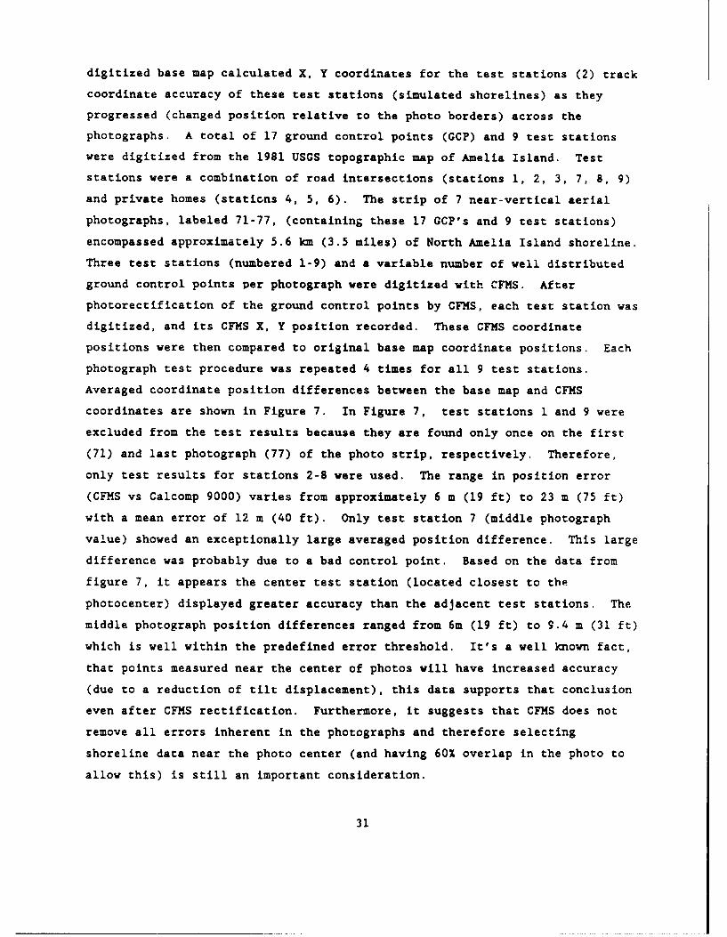
coordinates are shown in Figure 7. In Figure 7, test stations 1 and 9 were

excluded from the test results because they are found only once on the first

(71) and last photograph (77) of the photo strip, respectively. Therefore,

only test results for stations 2-8 were used. The range in position error

(CFMS vs Calcomp 9000) varies from approximately 6 m (19 ft) to 23 m (75 ft)

with a mean error of 12 m (40 ft). Only test station 7 (middle photograph

value) showed an exceptionally large averaged position difference. This large

difference was probably due to a bad control point. Based on the data from

figure 7, it appears the center test station (located closest to the

photocenter) displayed greater accuracy than the adjacent test stations. The

middle photograph position differences ranged from 6m (19 ft) to 9.4 m (31 ft)

which is well within the predefined error threshold. It's a well known fact,

that points measured near the center of photos will have increased accuracy

(due to a reduction of tilt displacement), this data supports that conclusion

even after CFMS rectification. Furthermore, it suggests that CFMS does not

remove all errors inherent in the photographs and therefore selecting

shoreline data near the photo center (and having 60% overlap in the photo to

allow this) is still an important consideration.

31

0I-

00

,__ _m 0 c

a.-, a 1. Od

LI.

1 Ct) N I)

0 >

LU)0 00

LU =..

a. 0 A w

0 0 0 A

*0 -

C u

0 0

0 00..a. a.

00000000

32

THE BRIDGING CONCEPT

50. Pristine areas of coastal shorelines often lack sufficient ground

control points, and large scale photos have limited ground control coverage,

prohibiting accurate digitization of the shoreline. Selection of improper

control points will adversely affect the accuracy of shoreline measurements.

Objects selected for reference points (ground control points) have to have

stable locations that do not move with time from natural or man-made causes.

Selection of these reference points can be accomplished by the naked eye, or

by stereoscopic equipment, when necessary. An example of good ground control

points are intersecting centerlines of paved street road intersections,

sidewalks and/or the corners of buildings at ground level.

51. Bridging allows a maximum of three photographs, with insufficient

ground control, to be "passed" over without sacrificing accuracy needed to

compute the shoreline position. Those areas lacking sufficient ground control

are assigned "pass" points, providing continuous continuity to the photo

strip. A pass point is any non &round control point (tree, rocks, etc.) which

can be found from one photograph to the next photograph (passed). inis

bridging process is superceded by a procedure called Collect. Collect permits

the measurement of photo coordinates of control and pass points from air

photos in a strip. Ground control and pass points are first assigned

sequential identification numbers. All points and photos must be numb-red

correctly and consistently, and all photo measurements must be as accurate as

possible. Errors introduced in this step, will be passed on to subsequent

steps (i.e. Bridge). These ground coordinates are then used in Bridge to

extend or densify the ground coordinate network. The CFMS users manual' gives

the following explanation of bridging: "Bridge connects the photo coordinates

to form a strip and then computes ground coordinates for each measured pass

point. Bridge performs a least squares transformation to create a set of

common coordinates for the entire strip. Finally, individual GCP files are

created which contain the coordinates of all points found on a given photo.

These files can then used to produce map overlays from the photos. Bridge

1 Center for Remote Sensing and Mapping Science, Department of Geography,University of Georgia, 1989, COASTAL FEATURES MAPPING SYSTEM, Athens Georgia.

33

does not perform a full aerotriangulation solution based on X, Y and Z terrain

coordinates. Consequently, the program does not account for terrain relief or

correct for earth curvature effects". For this reason, accuracy of the

solution is most reliable when strips are limited in size to 5 photographs and

terrain relief is minimal. Two of the five photographs (one on each end) must

have stable GCP's. The bridging across the three remaining photographs is

performed with a combination of pass and ground control points.

Bridgin2 (Ground control points on both ends)

52. As suggested above, a maximum of 3 photographs can be bridged.

This bridging process for 3 photographs, actually involves 5 photographs. The

first and fifth photographs contain ground control points (at least, 4 each),

tied together by the 3 middle photographs being bridged. A mosaic of 5

photographs were assembled to test CFMS's ability to calculate X, Y

coordinates for 5 test stations (2-6) on the bridged photos. Figure 8 bridges

5 photographs. Figure 9 bridges 4 photographs, and Figure 10 bridges 3

photographs. iiL general, results from these three bridging tests are

consistently within +/- 12m (40 ft) (accuracy of original base map), with

directional errors similar to results found in Figure 8 (GCP's on all

photographs). This suggests, that position coordinate accuracy is not lost by

the bridging process.

Bridaing (Ground control points on one end)

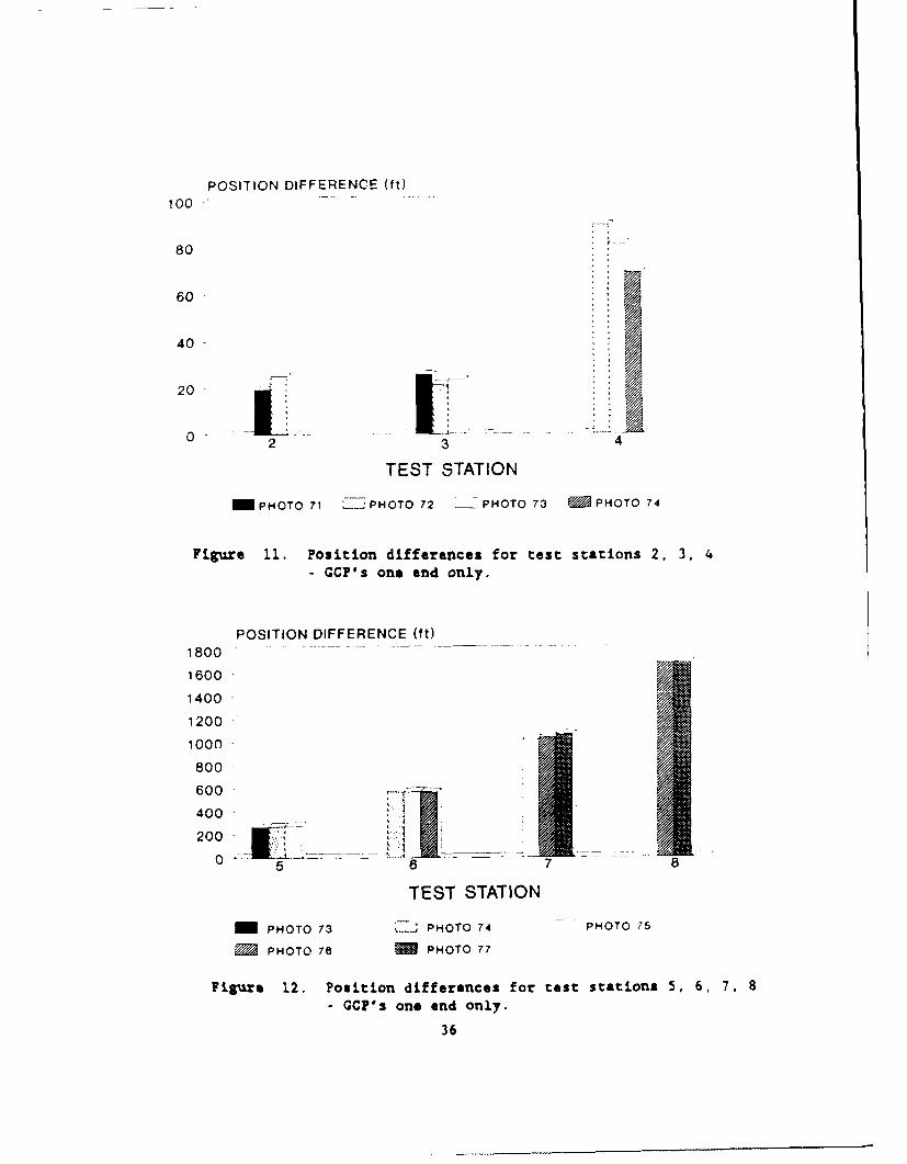
53. The CFMS bridging program was designed for situations where control

points could be located at each end of the photo strip. Control points on one

end only, cause coordinate position errors to increase rapidly with distance

from ground control points. As an experiment, a strip of 7 photographs were

bridged (in one direction) with 7 control points starting on the first

photograph. As you move away from the first photo, the number of GCP's become

smaller eventually terminating, leaving only pass points to calculate X, Y

positions of test stations. The results are shown in Figures 11 and 12.

Position differences from test stations 2, 3, 4 range from 6 m (19 ft) to 27 m

34

POSITION OIFFERENCE 111)80

80

40

20

0 i 2 3 5

TEST STATION

m PHOTO 71 Z PHOTO 72 PHOTO 73

M PHOTO 74 PHOTO 75

Figure 8. Position differences-Bridging 5 photographs

POSITION DIFFERENCE (t)80-

60

2 3 4

TEST STATION

M PHOTO 71 =PHOTO 72 - PHOTO 73 PHOTO 74

Figure 9. Position differences-Bridging 4 photographs

POSITION DIFFERENCE (t0

so -

80

20

40

3 4

TEST STATION

PHOTO 71 = PHOTO 72 PHOTO 73

Figure 10. Position differences-Bridging 3 photographs

35

POSITION DIFFERENCE 00t100

80

60

40

20

L0Lo2 3 4

TEST STATION

=PHOTO 71 ~.PHOTO 72 ~PHOTO 73 ~PHOTO 74

Figure 11. Position differences for test stations 2, 3. 4- GCP's one end only.

POSITION DIFFERENCE (ft)1800

1600

1400

1 200

1000

800

600

0

TEST STATION

MPHOTO 73 =j PHOTO 74 PHOTO 75

M PHOTO 76 20PHOTO 77

Figure 1.2. Position differences for test stations 5, 6, 7. 8- GCP's one end only.

36

(90 ft) and test stations 5, 6, 7, 8 range from 61 m (200 ft) to approximately

503 m (1650 ft) respectively. Clearly, one ended bridging should be limited

to 2-3 photos beyond the original ground control point photograph and should

be performed only when no other option exists.

37

PART V: SUMMARY AND CONCLUSIONS

54. In any mapping task, the accuracy of the final map producc and its

usefulness for quantitative analysis are determined in large part by the

quality of ground control points (GCP's) employed during compilation. Since

many coastal areas are subject to frequent change, it is often difficult to

fulfill the optimum requirements for ground control when mapping from aerial

photographs. For this reason, a series of tests was devised to evaluate the

accuracy of the Coastal Feature Mapping System (CFMS) for typical shoreline

mapping applications encountered by the Corps of Engineers. Major variables

tested included the number of ground control points employed in the solution

and their distribution. Ground control point3 digitized from 1:24,000 scale

USGS topographic maps were used in various combinations to orient 1:9600 scale

aerial photographs for coordinate retrieval. It was found that the accuracy

of X, Y coordinates determined from the photos is governed by the distribution

and accuracy of GCP's. Maximum accuracy is obtained when all measured points

are within the area bounded by the GCP's. Although at least four GCP's are

required for the solution, additional points allow possible mistakes to be

identified and corrected interactively. In all tests, the errors were

consistent with those associated with 1:24,000 scale base map as defined by

National Map Accuracy Standards. Measurements of shoreline points contained

in a strip of several photographs indicated that directional errors were

smaller for points located near the center of each photograph. This suggests

that positions of shorelines and other features digitized in the central

portions of the photographs are likely to be more accurate than those measured

on the margins. The unique capability of the CFMS to "bridge" measurements

across areas with little or no ground control was also evaluated. The tests

demonstrated that positional accuracy of digitized points could be maintained

over as many as three photographs as long as the photos on both ends of the

strip were well-controlled. Bridging beyond the control is not recommended.

The CFMS solution relies entirely upon the accuracy of the GCP's employed, the

photo scale and photo coordinate measurement error. With this in mind,

several basic principles must be recognized during a mapping operation: (1)

the accuracy of base map GCP location is a major factor controlling accuracy

of the CFMS solution, (2) minimum of four well-defined GCP's located in the

38

corners or margins of the photo are required to orient the photograph, and (3)

each GCP location should be digitized several times and the coordinates

averaged so as to minimize inaccuracies and errors in measurement. The users

guide (Welch, 1990) contained adequate information about overall program

operation, but lacked sufficient guidance for first time users. It assumes

the operator is knowledgeable about basic photogrammetric and aerial photo

mapping procedures. For more information on CFMS contact the Coastal Geology

Unit, Coastal Structures and Evaluation Branch, Engineering Development

Division, Coastal Engineering Research Center, U.S. Army Engineer Waterways

Experiment Station, Vicksburg, MS.

39

REFERENCES

Anders, F.J. and S.P. Leatherman, 1982. "Mapping Techniques and HistoricalShoreline Analysis - Nauset Spit, Massachusetts", In O.C. Farquhar, ed.,Geotechnology in Massachusetts, Amherst, MA, p 501-509.

Anders, F.J., D.W. Reed, and E.P. Meisburger, 1990. "Shoreline Movements,

Report 3: Tybee Island Georgia, to Cape Fear, North Carolina, 1851 - 1983", US

Army Engineers, Technical Report, CERC-83-1, 177 pg.

Byrnes, M.R., K.J. Gingerich, S.M. Kimball, and G.R. Thomas, 1989. "Temporal

and Spatial Variations in Shoreline Migration Rates, Metompkin Island,Virginia", In Barrier Islands: Process and Management, D.K. Stauble and O.T

Magoon editors, Coastal Zone 89, ASCE, pg 78-92.

Ellis, Melvin Y., editor, 1978. "Coastal Mapping Handbook", U.S. Dept. of theInterior, Geological Survey; U.S. Dept. of Commerce, National Ocean Survey;U.S. Gov't Printing Office, 199 pg.

Everts, C.H., J.P. Battley, and P.N. Gibson, 1983. "Shoreline Movements,Report 1: Cape Henry, Virginia, to Cape Hatteras, North Carolina, 1849-1980",US Army Engineers, Technical Report, CERC-83-1, 111 pg.

Knowles, S.C. and L.T. Gorman, (in press). "Summary and Assessment ofHistoric Data: St. Marys Entrance and Vicinity, Florida-Georgia", US Army

Engineers, Technical Report, CERC-90-

Langfelder, L.J., D.B. Stafford, and M. Amein, 1970. "Coastal Erosion inNorth Carolina", ASCE Jour. Waterways and Harbors Div, WW2, p 531-545.

Leatherman, Stephen P., 1983. "Shoreline Mapping: A Comparison of

Techniques", Shore and Beach, No. 7, p 28-33.

Moffitt, Francis H., 1969. "History of Shore Growth from Aerial Photographs",

Shore and Beach, No. 4, p 23-27.

Shalowitz, Aaron L., 1964. "Shoreline and Sea Boundaries", V 1, Pub. 10-1, USDept. of Commerce, Coast and Geodetic Survey, US. Gov't Printing Office, 420

pg.

Wong, K.W., 1980. "Basic Mathematics of Photogrammetry", In: Slama, ChesterC. editor, Manual of Photogrammetry, 4th Ed., American Soc. of Photogrammetry,

Falls Church, VA., 1056 pg.

Stafford, D.B. and Langfelder, J., 1971. "Air Photo Survey of CoastalErosion", Photogrammetric Engineering, V. 37, p 565-575.

Stafford, Donald B., 1971. "An Aerial Photographic Technique for Beach

Erosion Surveys in North Carolina", US Army Engineers, CERC, TM-36, 115 pg.

40

Tanner, William F., 1978. "Standards for Measuring Shoreline Change",

Proceedings of a Workshop, Florida State Univ., 85 pg.

Wolf, Paul R., 1983. Elements of Photogrammetry, 2nd Ed., New York, McGraw-

Hill, 628 pg.

Welch, R.A., 1990. "Coastal Features Mapping System (CFMS)," The Center for

Remote Sensing and Mapping Sciences, The University of Georgia, Athens,

Georgia.

U.S. Army Corps of Engineers, 1984. "Feasibility Report with Environmental

Impact Statement for Beach Erosion Control, Nassau County, Florida (Amelia

Island)," Corps of Engineers, South Atlantic Div., Jacksonville District, FL.

41

APPENDIX A: Shoreline Change Along a Developed Coast:

North Amelia Island, i7lorida

The Study Area

55. In order to evaluate CFMS, a section of shoreline along the

northern end of Amelia Island, Florida was digitized and mapped. Aerial

photography obtained in 1988 was the primary data source used in this

evaluation. The shoreline mapped from this photography was compared with

historical shorelines developed from maps and other near vertical photo sets.

The base map used in this application was the 1981 (photorevised 1988) US

Geological Survey 1:24,000 topographic map (Fernandina Quadrangle). The site,

photography, and base map represent typical information available for Corps of

Engineers shoreline change mapping applications.

56. St. Marys Entrance is a tidal inlet separating Cumberland Island,

Georgia and Amelia Island, Florida (Figure 2). The inlet is about 48 km (30

miles) north northeast of Jacksonville Florida, and 48 km (30 miles) south of

Brunswick, Georgia. A federally maintained e.,--anca .hannel, accessing the

Intracoastal Waterway, ports at Fernandina, Florida and St. Marys, Georgia,

and the U.S. Naval Submarine Base at Kings Bay. Historically the main ebb

tidal channel for St.Hary's Inlet hugged the shore of Amelia Island. By the

1870's the channel bifurcated around a sand bar deposited across the inlet.

This bar was located 3.2 km (2 miles) offshore at about the 2.4 m (8 ft) depth

contour. Inlet stabilization began with construction of the north jetty in

1881. Major changes in inlet configuration had occurred by 1905 when the

jetties were complete. One main channel was confined between the jetties and

the northern channel was cutoff by the north jetty. Kings Bay Naval Submarine

Support Base continuously grew since the 1950's and by 1980 the channel depth

was increased to -12 m (-40 ft) low water (MLW). In order for larger Trident-

class submarines to use the Kings Bay facilities, project channel dimensions

had to be modified. By the mid-1980's, channel dimensions were increased to a

depth of -15 m (-49 ft) MLW, a width of 150 m (500 ft), and a channel length

of 15087 m (49,500 ft). As a result, 1.68 million cu m (2.2 million cu yds)

of sand, was placed along 5.8 km (3.6 miles) of north Amelia Island beach

(Knowles and Gorman, in press).

57. The project area is part of the southeast Atlantic Coastal Plain

Al

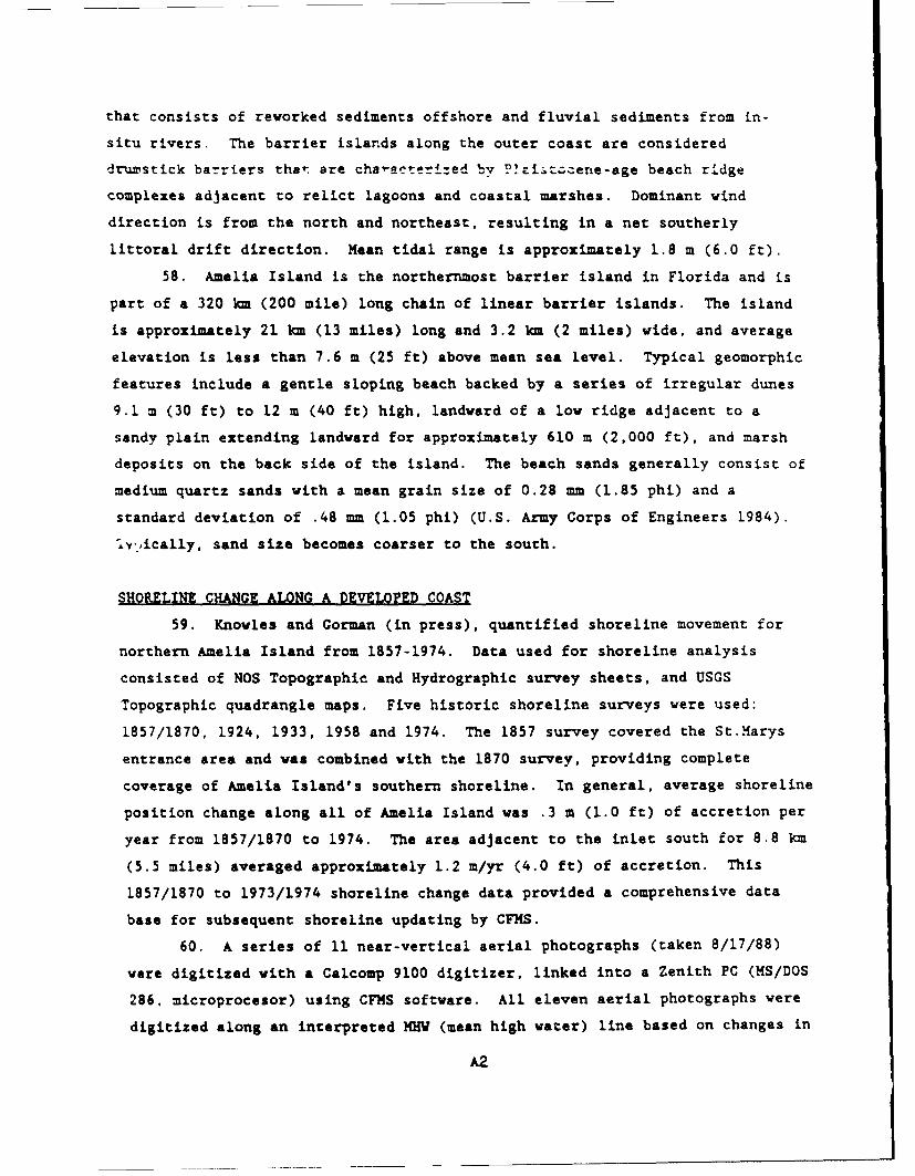
that consists of reworked sediments offshore and fluvial sediments from in-

situ rivers. The barrier islands along the outer coast are considered

drumstick barriers tha' are cha-acterized by F!zi cene-age beach ridge

complexes adjacent to relict lagoons and coastal marshes. Dominant wind

direction is from the north and northeast, resulting in a net southerly

littoral drift direction. Mean tidal range is approximately 1.8 m (6.0 ft).

58. Amelia Island is the northernmost barrier island in Florida and is

part of a 320 km (200 mile) long chain of linear barrier islands. The island

is approximately 21 km (13 miles) long and 3.2 km (2 miles) wide, and average

elevation is less than 7.6 m (25 ft) above mean sea level. Typical geomorphic

features include a gentle sloping beach backed by a series of irregular dunes

9.1 m (30 ft) to 12 m (40 ft) high, landward of a low ridge adjacent to a

sandy plain extending landward for approximately 610 m (2,000 ft), and marsh

deposits on the back side of the island. The beach sands generally consist of

medium quartz sands with a mean grain size of 0.28 mm (1.85 phi) and a

standard deviation of .48 mm (1.05 phi) (U.S. Army Corps of Engineers 1984).

l.v'ically, sand size becomes coarser to the south.

SHORELINE CHANGE ALONG A DEVELOPED COAST

59. Knowles and Gorman (in press), quantified shoreline movement for

northern Amelia Island from 1857-1974. Data used for shoreline analysis

consisted of NOS Topographic and Hydrographic survey sheets, and USGS

Topographic quadrangle maps. Five historic shoreline surveys were used:

1857/1870, 1924, 1933, 1958 and 1974. The 1857 survey covered the St.Marys

entrance area and was combined with the 1870 survey, providing complete

coverage of Amelia Island's southern shoreline. In general, average shoreline

position change along all of Amelia Island was .3 m (1.0 ft) of accretion per

year from 1857/1870 to 1974. The area adjacent to the inlet south for 8.8 km

(5.5 miles) averaged approximately 1.2 m/yr (4.0 ft) of accretion. This

1857/1870 to 1973/1974 shoreline change data provided a comprehensive data

base for subsequent shoreline updating by CFMS.

60. A series of 11 near-vertical aerial photographs (taken 8/17/88)

were digitized with a Calcomp 9100 digitizer, linked into a Zenith PC (MS/DOS

286, microprocesor) using CFMS software. All eleven aerial photographs were

digitized along an interpreted MHW (mean high water) line based on changes in

A2

color as described by Langfelder and Stafford 1971. Standard aerial

photography provides approximately 60 percent overlap from one photograph to

the next. If the entire shoreline on each photo is di.itize 4 , this rhoreline

overlap must be edited out after digitization is complete. This editing

procedure, produces a single continuous set of X, Y coordinates representing

the 1988 shoreline position. All shoreline data was then entered into COAST

(discussed earlier). Shoreline position change statistics were calculated

along transects spaced 300 feet along the "average shoreline". Figure 13

shows a 1988 CFKS digitized shoreline, along with COAST generated shoreline

statistics. Segmented shoreline data for 1857/1870 were appended together to

represent one continous coastline for this time period. The mean shoreline

movement, from St. Marys Inlet south (8 km, 5.5 miles) from 1974-1988 was

approximately 1.43 m (4.7 feet) accretion per year. This accretion may

represent landward movement of ebb-tidal shoals after jetty construction,

and/or subsequent sand placement of beach material during St. Marys entrance

channel deepening for the larger Trident-class submarines. Standard deviation

reflects variablik , 'oo,it the average mean change rate. Along northern

Amelia Island, adjacent to the jetties, standard deviation values are large.

Where standard deviations are high, shorelines tend to be variable, thus

usefulness of average rate for pxedicting future shoreline position is

reduced. Because of the variable accuracy, results from shoreline position

change analysis are more suited for characterizing general trends and relative

comparison of coastal reaches. Quantitative use of the analysis results

should be used with caution.

A3

AMELIA ISLAND STUDY

MEAN SHORELINE S) 1REUNE MOVEMENTSHOREUNE MOVEMENT MOVEMENT FEET PER YEAR

FROM 1857-1986 FT. PER YEAR STANDARD DEVIATION 1974 VS 1988

-30 0 30 -30 0 30 -30 0 30a

- "'..8174

187-174 -11157-1974

V1 AMELIA!13 ISLAND

2L

4-\

7:7

-/

Figure 13. Updated 1988 Amelia Island shoreline, Mean ShorelineMovement, Standard Deviation, and Absolute ShorelineMovement.

A4