by Didier Besnard, Francis H. Harlow, Rick Rauenzahn, · by Didier Besnard, w hen the interface between two materials experiences strong accelerative Francis H. Harlow, or shearing

by Didier Besnard, w hen the interface between two materials experiences strong accelerative

Francis H. Harlow, or shearing forces, the inevitable results are instability, turbulence, andthe mixing of materials, momentum, and energy. One of the most impor-

Norman L. Johnson, tant and exciting breakthroughs in our understanding of these disruptive

Rick Rauenzahn, processes has been the recent discovery that the features of the processes often are

and Jonathan Wolfe independent of the initial interface perturbations. This discovery is so important thatscientists at Los Alamos National Laboratory, the California Institute of Technology,

Los Alamos Science Special Issue 1987

the Atomic Weapons Research Establishment in Great Britain, Lawrence LivermoreNational Laboratory, as well as scientists in France, and no doubt in the Soviet Union,are working hard to confirm and extend this new understanding experimentally.

Theoretical analyses are likewise showing a firm basis for this astonishing dis-covery. Two types of theory are being employed, gradually combined, and evenproved essentially equivalent. These are the multifield-interpenetration approach andthe single-field turbulence approach. Even brute-force hydrodynamics calculations aredemonstrating this same property of independence from initial perturbation.

The consequences for developments in such main-line Laboratory projects asinertial-confinement fusion are profound. Our entire view of material mixing, tur-bulence shear impedance, and energy transport has undergone a revolutionary shift toqualitatively different directions.

What is the physical essence of this new way of thinking? No matter how

145

Turbulence

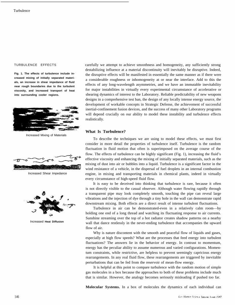
TURBULENCE EFFECTS

Fig. 1. The effects of turbulence include in-

creased mixing of initially separated materi-

als, an increase in shear impedance of fluid

near rough boundaries due to the turbulent

viscosity, and increased transport of heat

into surrounding cooler regions.

Increased Mixing of Materials

Increased Shear Impedance

Increased Heat Diffusion

carefully we attempt to achieve smoothness and homogeneity, any sufficiently strongdestabilizing influence at a material discontinuity will inevitably be disruptive. Indeed,the disruptive effects will be manifested in essentially the same manner as if there werea considerable roughness or inhomogeneity at or near the interface. Add to this theeffects of any long-wavelength asymmetries, and we have an immutable inevitabilityfor major instabilities in virtually every experimental circumstance of accelerative orshearing dynamics of interest to the Laboratory. Reliable predictability of new weaponsdesigns in a comprehensive test ban, the design of any locally intense energy source, thedevelopment of workable concepts in Strategic Defense, the achievement of successfulinertial-confinement fusion devices, and the success of many other Laboratory programswill depend crucially on our ability to model these instability and turbulence effectsrealistically.

What Is Turbulence?

To describe the techniques we are using to model these effects, we must firstconsider in more detail the properties of turbulence itself. Turbulence is the randomfluctuation in fluid motion that often is superimposed on the average course of the

flow. The effects of turbulence can be highly significant (Fig. 1), increasing the fluid’seffective viscosity and enhancing the mixing of initially separated materials, such as themixing of dust into air or bubbles into a liquid. Turbulence is a significant factor in thewind resistance of a vehicle, in the dispersal of fuel droplets in an internal combustionengine, in mixing and transporting materials in chemical plants, indeed in virtuallyevery circumstance of high-speed fluid flow.

It is easy to be deceived into thinking that turbulence is rare, because it oftenis not directly visible to the casual observer. Although water flowing rapidly througha transparent pipe may look completely smooth, touching the pipe can reveal largevibrations and the injection of dye through a tiny hole in the wall can demonstrate rapiddownstream mixing. Both effects are a direct result of intense turbulent fluctuations.

Turbulence in air can be demonstrated-even in a relatively calm room—byholding one end of a long thread and watching its fluctuating response to air currents.Sunshine streaming over the top of a hot radiator creates shadow patterns on a nearbywall that dance restlessly in the never-ending turbulence that accompanies the upwardflow of air.

Why is nature discontent with the smooth and peaceful flow of liquids and gases,especially at high flow speeds? What are the processes that feed energy into turbulentfluctuations? The answers lie in the behavior of energy. In contrast to momentum,energy has the peculiar ability to assume numerous and varied configurations. Momen-tum constraints, while restrictive, are helpless to prevent seemingly capricious energyrearrangements. In any real fluid flow, these rearrangements are triggered by inevitableperturbations that can be fed from the reservoir of mean-flow energy.

It is helpful at this point to compare turbulence with the random motion of simplegas molecules in a box because the approaches to both of these problems include muchthat is similar. However, the analogy becomes seriously misleading if pushed too far.

Molecular Systems. In a box of molecules the dynamics of each individual can

146

Turbulence

be described quite accurately by Newton’s laws. Yet we seldom try to analyze thecomplex interactions of all the trajectories, which are seemingly capable of very chaoticbehavior. Instead, we appeal to the remarkably organized mean properties of the motion,identifying such useful variables as density, pressure, temperature, and fluid velocity.

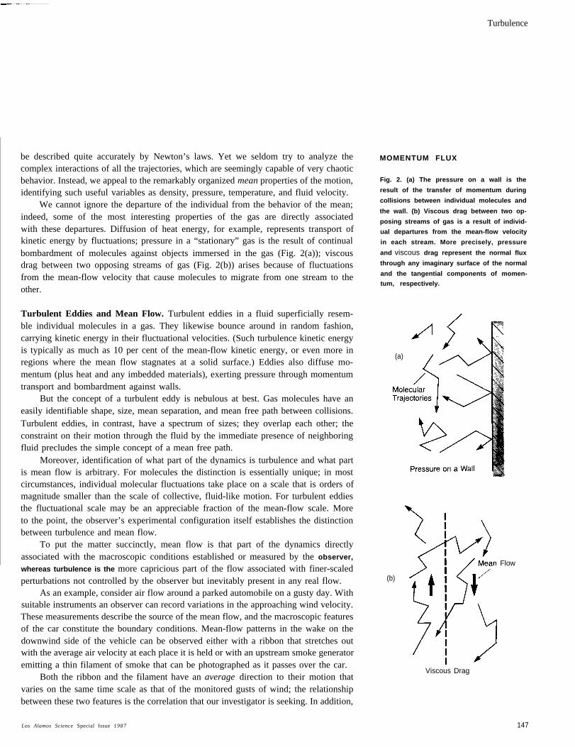
We cannot ignore the departure of the individual from the behavior of the mean;indeed, some of the most interesting properties of the gas are directly associatedwith these departures. Diffusion of heat energy, for example, represents transport ofkinetic energy by fluctuations; pressure in a “stationary” gas is the result of continualbombardment of molecules against objects immersed in the gas (Fig. 2(a)); viscousdrag between two opposing streams of gas (Fig. 2(b)) arises because of fluctuationsfrom the mean-flow velocity that cause molecules to migrate from one stream to theother.

Turbulent Eddies and Mean Flow. Turbulent eddies in a fluid superficially resem-ble individual molecules in a gas. They likewise bounce around in random fashion,carrying kinetic energy in their fluctuational velocities. (Such turbulence kinetic energyis typically as much as 10 per cent of the mean-flow kinetic energy, or even more inregions where the mean flow stagnates at a solid surface.) Eddies also diffuse mo-mentum (plus heat and any imbedded materials), exerting pressure through momentumtransport and bombardment against walls.

But the concept of a turbulent eddy is nebulous at best. Gas molecules have aneasily identifiable shape, size, mean separation, and mean free path between collisions.Turbulent eddies, in contrast, have a spectrum of sizes; they overlap each other; theconstraint on their motion through the fluid by the immediate presence of neighboringfluid precludes the simple concept of a mean free path.

Moreover, identification of what part of the dynamics is turbulence and what partis mean flow is arbitrary. For molecules the distinction is essentially unique; in mostcircumstances, individual molecular fluctuations take place on a scale that is orders ofmagnitude smaller than the scale of collective, fluid-like motion. For turbulent eddiesthe fluctuational scale may be an appreciable fraction of the mean-flow scale. Moreto the point, the observer’s experimental configuration itself establishes the distinctionbetween turbulence and mean flow.

To put the matter succinctly, mean flow is that part of the dynamics directlyassociated with the macroscopic conditions established or measured by the observer,

whereas turbulence is the more capricious part of the flow associated with finer-scaledperturbations not controlled by the observer but inevitably present in any real flow.

As an example, consider air flow around a parked automobile on a gusty day. Withsuitable instruments an observer can record variations in the approaching wind velocity.These measurements describe the source of the mean flow, and the macroscopic featuresof the car constitute the boundary conditions. Mean-flow patterns in the wake on thedownwind side of the vehicle can be observed either with a ribbon that stretches outwith the average air velocity at each place it is held or with an upstream smoke generatoremitting a thin filament of smoke that can be photographed as it passes over the car.

Both the ribbon and the filament have an average direction to their motion thatvaries on the same time scale as that of the monitored gusts of wind; the relationshipbetween these two features is the correlation that our investigator is seeking. In addition,

MOMENTUM FLUX

Fig. 2. (a) The pressure on a wall is the

result of the transfer of momentum during

collisions between individual molecules and

the wall. (b) Viscous drag between two op-

posing streams of gas is a result of individ-

ual departures from the mean-flow velocity

in each stream. More precisely, pressure

and viscous drag represent the normal flux

through any imaginary surface of the normal

and the tangential components of momen-

tum, respectively.

(a)

(b)

Viscous Drag

Flow

Los Alamos Science Special Issue 1987 147

Turbulence

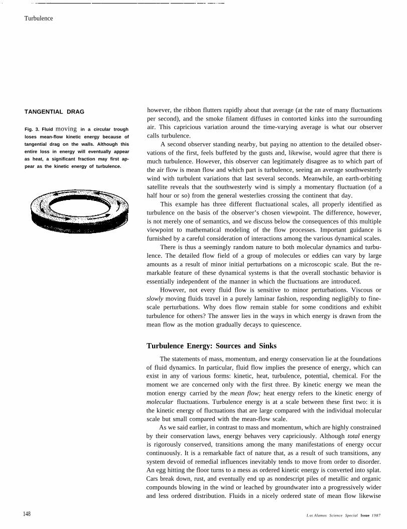
TANGENTIAL DRAG

Fig. 3. Fluid moving in a circular trough

loses mean-flow kinetic energy because of

tangential drag on the walls. Although this

entire loss in energy will eventually appear

as heat, a significant fraction may first ap-

pear as the kinetic energy of turbulence.

however, the ribbon flutters rapidly about that average (at the rate of many fluctuationsper second), and the smoke filament diffuses in contorted kinks into the surroundingair. This capricious variation around the time-varying average is what our observercalls turbulence.

A second observer standing nearby, but paying no attention to the detailed obser-vations of the first, feels buffeted by the gusts and, likewise, would agree that there ismuch turbulence. However, this observer can legitimately disagree as to which part ofthe air flow is mean flow and which part is turbulence, seeing an average southwesterlywind with turbulent variations that last several seconds. Meanwhile, an earth-orbitingsatellite reveals that the southwesterly wind is simply a momentary fluctuation (of ahalf hour or so) from the general westerlies crossing the continent that day.

This example has three different fluctuational scales, all properly identified asturbulence on the basis of the observer’s chosen viewpoint. The difference, however,is not merely one of semantics, and we discuss below the consequences of this multipleviewpoint to mathematical modeling of the flow processes. Important guidance isfurnished by a careful consideration of interactions among the various dynamical scales.

There is thus a seemingly random nature to both molecular dynamics and turbu-lence. The detailed flow field of a group of molecules or eddies can vary by largeamounts as a result of minor initial perturbations on a microscopic scale. But the re-markable feature of these dynamical systems is that the overall stochastic behavior isessentially independent of the manner in which the fluctuations are introduced.

However, not every fluid flow is sensitive to minor perturbations. Viscous orslowly moving fluids travel in a purely laminar fashion, responding negligibly to fine-scale perturbations. Why does flow remain stable for some conditions and exhibitturbulence for others? The answer lies in the ways in which energy is drawn from themean flow as the motion gradually decays to quiescence.

Turbulence Energy: Sources and Sinks

The statements of mass, momentum, and energy conservation lie at the foundationsof fluid dynamics. In particular, fluid flow implies the presence of energy, which canexist in any of various forms: kinetic, heat, turbulence, potential, chemical. For themoment we are concerned only with the first three. By kinetic energy we mean themotion energy carried by the mean flow; heat energy refers to the kinetic energy ofmolecular fluctuations. Turbulence energy is at a scale between these first two: it isthe kinetic energy of fluctuations that are large compared with the individual molecularscale but small compared with the mean-flow scale.

As we said earlier, in contrast to mass and momentum, which are highly constrainedby their conservation laws, energy behaves very capriciously. Although total energyis rigorously conserved, transitions among the many manifestations of energy occurcontinuously. It is a remarkable fact of nature that, as a result of such transitions, anysystem devoid of remedial influences inevitably tends to move from order to disorder.An egg hitting the floor turns to a mess as ordered kinetic energy is converted into splat.Cars break down, rust, and eventually end up as nondescript piles of metallic and organiccompounds blowing in the wind or leached by groundwater into a progressively widerand less ordered distribution. Fluids in a nicely ordered state of mean flow likewise

148 L oS Alamos Science Special Issue 1987

Turbulence

Mean-Flow Kinetic Energy I

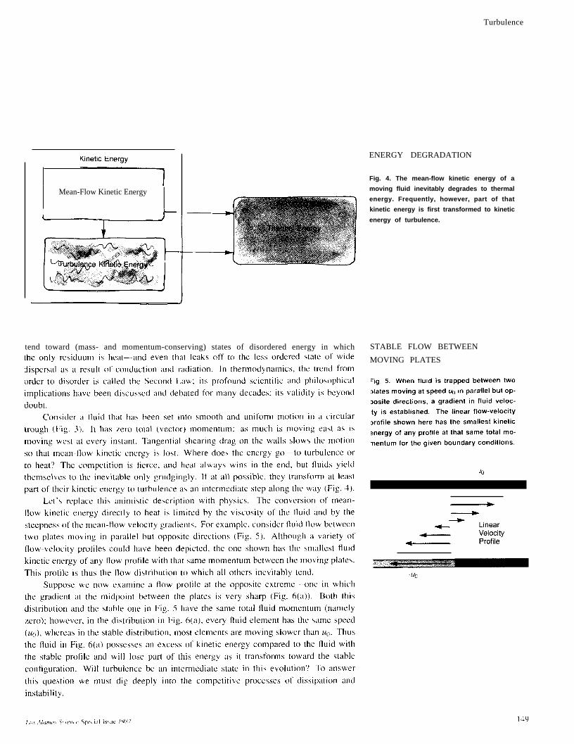
tend toward (mass- and momentum-conserving) states of disordered energy in which

ENERGY DEGRADATION

Fig. 4. The mean-flow kinetic energy of a

moving fluid inevitably degrades to thermal

energy. Frequently, however, part of that

kinetic energy is first transformed to kinetic

energy of turbulence.

STABLE FLOW BETWEEN

MOVING PLATES

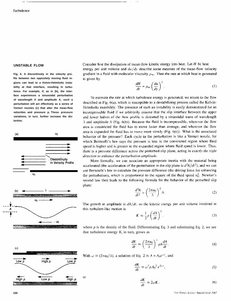
UNSTABLE FLOW

Fig, 6. A discontinuity in the velocity pro-

file between two oppositely moving fluid re-

gions can lead to a Kelvin-Helmholtz insta-

bility at that interface, resulting in turbu-

lence. For example, if, as in (b), the inter-

face experiences a sinusoidal perturbation

of wavelength X and amplitude A, such a

perturbation will act effectively as a series of

Venturi nozzles (c) that alter the mean-flow

velocities and pressure p. These pressure

variations, in turn, further increase the dis-

tortion.

(c)

where p is the density of the fluid. Differentiating Eq. 3 and substituting Eq. 2, we seethat turbulence energy K, in turn, grows as

or

(4)

(5)

150

Turbulence

(7)

Local InitialReynolds Pertur-Number bation

LOS Alamos Science Special Issue 1987 151

Turbulence

ReynoldsNumber

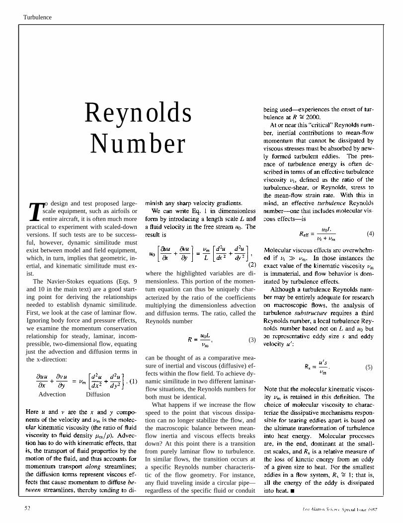
To design and test proposed large-scale equipment, such as airfoils orentire aircraft, it is often much more

practical to experiment with scaled-downversions. If such tests are to be success-ful, however, dynamic similitude mustexist between model and field equipment,which, in turn, implies that geometric, in-ertial, and kinematic similitude must ex-ist.

The Navier-Stokes equations (Eqs. 9and 10 in the main text) are a good start-ing point for deriving the relationshipsneeded to establish dynamic similitude.First, we look at the case of laminar flow.Ignoring body force and pressure effects,we examine the momentum conservationrelationship for steady, laminar, incom-pressible, two-dimensional flow, equatingjust the advection and diffusion terms inthe x-direction:

Advection Diffusion

where the highlighted variables are di-mensionless. This portion of the momen-tum equation can thus be uniquely char-acterized by the ratio of the coefficientsmultiplying the dimensionless advectionand diffusion terms. The ratio, called theReynolds number

(3)

can be thought of as a comparative mea-sure of inertial and viscous (diffusive) ef-fects within the flow field. To achieve dy-namic similitude in two different laminar-flow situations, the Reynolds numbers forboth must be identical.

What happens if we increase the flowspeed to the point that viscous dissipa-tion can no longer stabilize the flow, andthe macroscopic balance between mean-flow inertia and viscous effects breaksdown? At this point there is a transitionfrom purely laminar flow to turbulence.In similar flows, the transition occurs ata specific Reynolds number characteris-tic of the flow geometry. For instance,any fluid traveling inside a circular pipe—regardless of the specific fluid or conduit

(4)

(5)

Turbulence

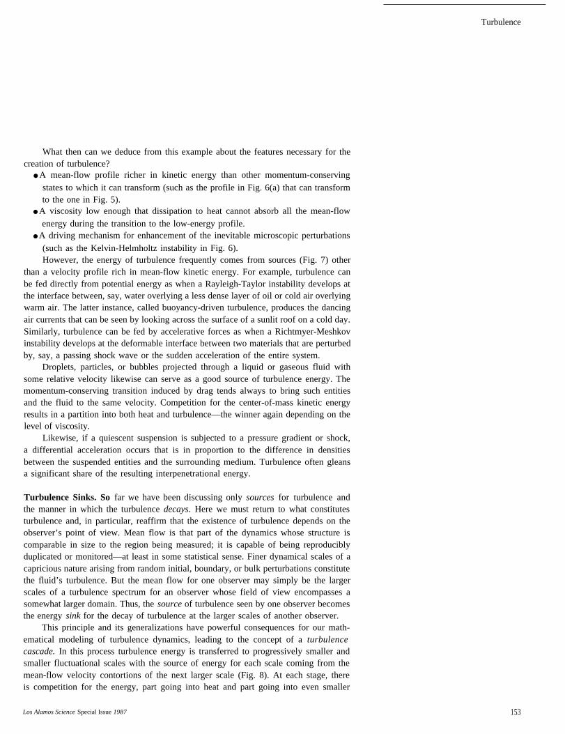
What then can we deduce from this example about the features necessary for thecreation of turbulence?

● A mean-flow profile richer in kinetic energy than other momentum-conservingstates to which it can transform (such as the profile in Fig. 6(a) that can transformto the one in Fig. 5).

● A viscosity low enough that dissipation to heat cannot absorb all the mean-flowenergy during the transition to the low-energy profile.

● A driving mechanism for enhancement of the inevitable microscopic perturbations(such as the Kelvin-Helmholtz instability in Fig. 6).However, the energy of turbulence frequently comes from sources (Fig. 7) other

than a velocity profile rich in mean-flow kinetic energy. For example, turbulence canbe fed directly from potential energy as when a Rayleigh-Taylor instability develops atthe interface between, say, water overlying a less dense layer of oil or cold air overlyingwarm air. The latter instance, called buoyancy-driven turbulence, produces the dancingair currents that can be seen by looking across the surface of a sunlit roof on a cold day.Similarly, turbulence can be fed by accelerative forces as when a Richtmyer-Meshkovinstability develops at the deformable interface between two materials that are perturbedby, say, a passing shock wave or the sudden acceleration of the entire system.

Droplets, particles, or bubbles projected through a liquid or gaseous fluid withsome relative velocity likewise can serve as a good source of turbulence energy. Themomentum-conserving transition induced by drag tends always to bring such entitiesand the fluid to the same velocity. Competition for the center-of-mass kinetic energyresults in a partition into both heat and turbulence—the winner again depending on thelevel of viscosity.

Likewise, if a quiescent suspension is subjected to a pressure gradient or shock,a differential acceleration occurs that is in proportion to the difference in densitiesbetween the suspended entities and the surrounding medium. Turbulence often gleansa significant share of the resulting interpenetrational energy.

Turbulence Sinks. So far we have been discussing only sources for turbulence andthe manner in which the turbulence decays. Here we must return to what constitutesturbulence and, in particular, reaffirm that the existence of turbulence depends on theobserver’s point of view. Mean flow is that part of the dynamics whose structure iscomparable in size to the region being measured; it is capable of being reproduciblyduplicated or monitored—at least in some statistical sense. Finer dynamical scales of acapricious nature arising from random initial, boundary, or bulk perturbations constitutethe fluid’s turbulence. But the mean flow for one observer may simply be the largerscales of a turbulence spectrum for an observer whose field of view encompasses asomewhat larger domain. Thus, the source of turbulence seen by one observer becomesthe energy sink for the decay of turbulence at the larger scales of another observer.

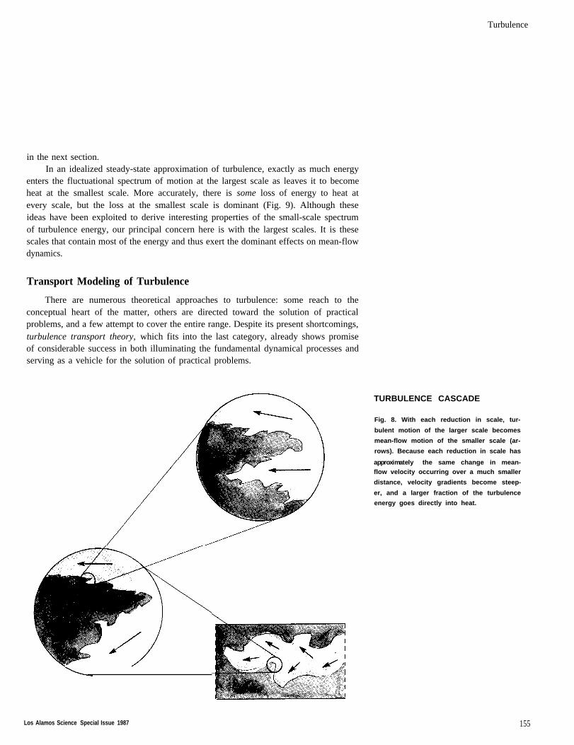
This principle and its generalizations have powerful consequences for our math-ematical modeling of turbulence dynamics, leading to the concept of a turbulencecascade. In this process turbulence energy is transferred to progressively smaller andsmaller fluctuational scales with the source of energy for each scale coming from themean-flow velocity contortions of the next larger scale (Fig. 8). At each stage, thereis competition for the energy, part going into heat and part going into even smaller


Turbulence

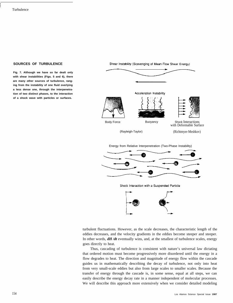
SOURCES OF TURBULENCE

Fig. 7. Although we have so far dealt only

with shear instabilities (Figs. 5 and 6), there

are many other sources of turbulence, rang-

ing from the instability of one fluid overlying

a less dense one, through the interpenetra-

tion of two distinct phases, to the interaction

of a shock wave with particles or surfaces.

Body Force Buoyancy

(Rayleigh-Taylor)

Shock Interactionswith Deformable Surface

(Richtmyer-Meshkov)

Energy from Relative Interpenetration (Two-Phase Instability)

turbulent fluctuations. However, as the scale decreases, the characteristic length of theeddies decreases, and the velocity gradients in the eddies become steeper and steeper.In other words, dH /dt eventually wins, and, at the smallest of turbulence scales, energygoes directly to heat.

Thus, cascading of turbulence is consistent with nature’s universal law dictatingthat ordered motion must become progressively more disordered until the energy in aflow degrades to heat. The direction and magnitude of energy flow within the cascadeguides us in mathematically describing the decay of turbulence, not only into heatfrom very small-scale eddies but also from large scales to smaller scales. Because thetransfer of energy through the cascade is, in some sense, equal at all steps, we caneasily describe the energy decay rate in a manner independent of molecular processes.We will describe this approach more extensively when we consider detailed modeling

154 Los Alamos Science Special Issue 1987

Turbulence

in the next section.In an idealized steady-state approximation of turbulence, exactly as much energy

enters the fluctuational spectrum of motion at the largest scale as leaves it to becomeheat at the smallest scale. More accurately, there is some loss of energy to heat atevery scale, but the loss at the smallest scale is dominant (Fig. 9). Although theseideas have been exploited to derive interesting properties of the small-scale spectrumof turbulence energy, our principal concern here is with the largest scales. It is thesescales that contain most of the energy and thus exert the dominant effects on mean-flowdynamics.

Transport Modeling of Turbulence

There are numerous theoretical approaches to turbulence: some reach to theconceptual heart of the matter, others are directed toward the solution of practicalproblems, and a few attempt to cover the entire range. Despite its present shortcomings,turbulence transport theory, which fits into the last category, already shows promiseof considerable success in both illuminating the fundamental dynamical processes andserving as a vehicle for the solution of practical problems.

TURBULENCE CASCADE

Fig. 8. With each reduction in scale, tur-

bulent motion of the larger scale becomes

mean-flow motion of the smaller scale (ar-

rows). Because each reduction in scale has

approximately the same change in mean-flow velocity occurring over a much smaller

distance, velocity gradients become steep-

er, and a larger fraction of the turbulence

energy goes directly into heat.


Turbulence

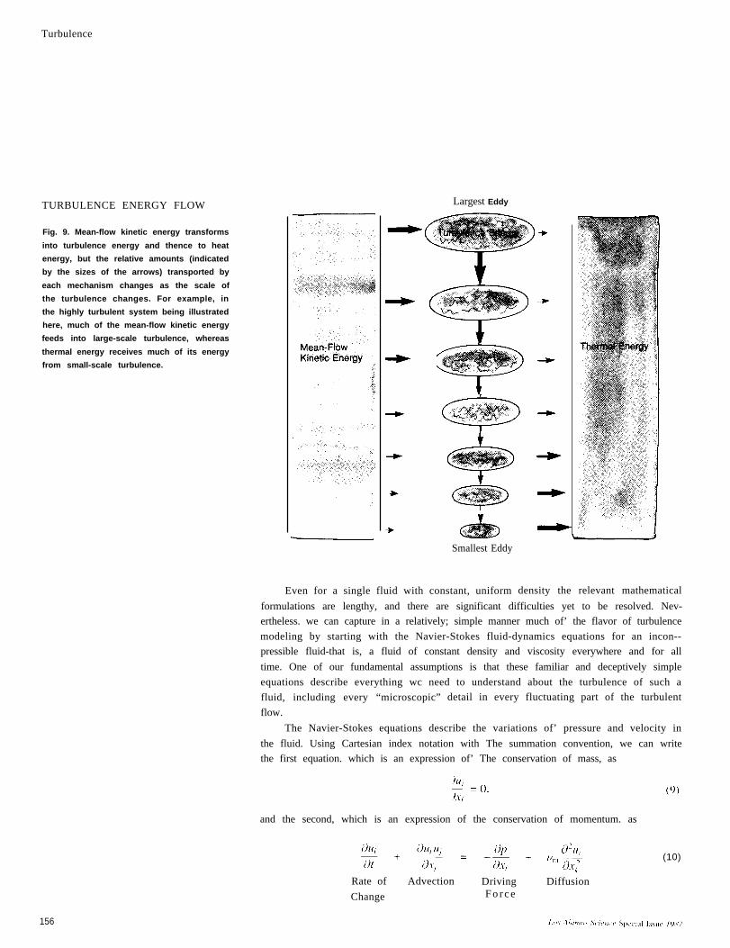
TURBULENCE ENERGY FLOW Largest Eddy

Fig. 9. Mean-flow kinetic energy transforms

into turbulence energy and thence to heat

energy, but the relative amounts (indicated

by the sizes of the arrows) transported by

each mechanism changes as the scale of

the turbulence changes. For example, in

the highly turbulent system being illustrated

here, much of the mean-flow kinetic energy

feeds into large-scale turbulence, whereas

thermal energy receives much of its energy

from small-scale turbulence.

Smallest Eddy

Even for a single fluid with constant, uniform density the relevant mathematical

formulations are lengthy, and there are significant difficulties yet to be resolved. Nev-

ertheless. we can capture in a relatively; simple manner much of’ the flavor of turbulence

modeling by starting with the Navier-Stokes fluid-dynamics equations for an incon--

pressible fluid-that is, a fluid of constant density and viscosity everywhere and for all

time. One of our fundamental assumptions is that these familiar and deceptively simple

equations describe everything wc need to understand about the turbulence of such a

fluid, including every “microscopic” detail in every fluctuating part of the turbulent

flow.

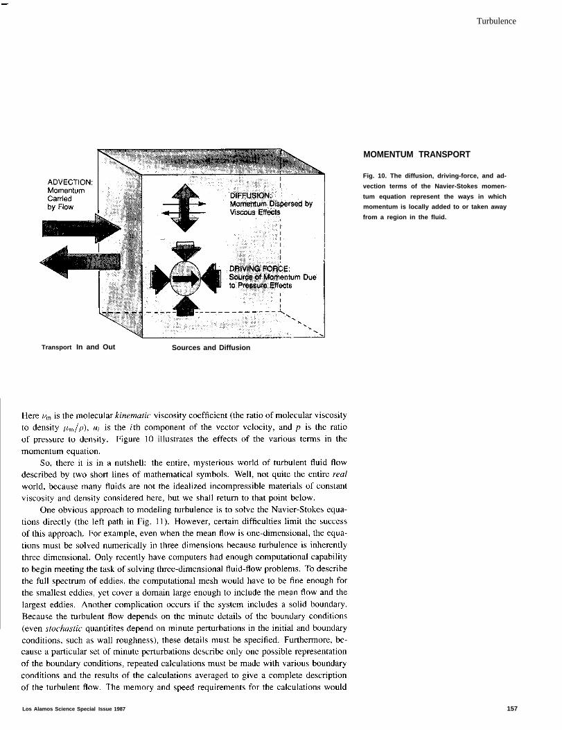
The Navier-Stokes equations describe the variations of’ pressure and velocity in

the fluid. Using Cartesian index notation with The summation convention, we can write

the first equation. which is an expression of’ The conservation of mass, as

and the second, which is an expression of the conservation of momentum. as

Rate of Advection Driving Diffusion

Change F o r c e

(10)

156

Turbulence

MOMENTUM TRANSPORT

Fig. 10. The diffusion, driving-force, and ad-

vection terms of the Navier-Stokes momen-

tum equation represent the ways in which

momentum is locally added to or taken away

from a region in the fluid.

Transport In and Out Sources and Diffusion


Turbulence

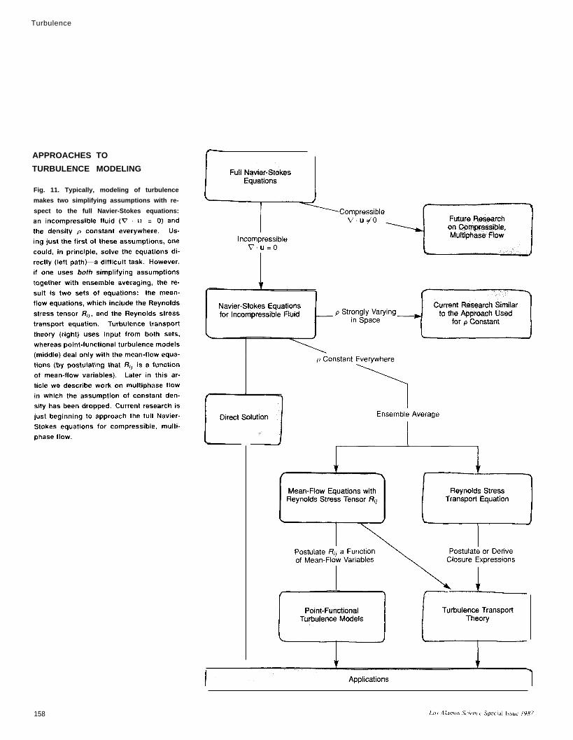
APPROACHES TO

TURBULENCE MODELING

Fig. 11. Typically, modeling of turbulence

makes two simplifying assumptions with re-

spect to the full Navier-Stokes equations:

158

Turbulence

Experiment 4

tax even the most powerful of our modem computers. If these calculations could beaccomplished, however, the advantage of a direct calculation of turbulence would bethat no approximations or empirical postulates are required.

Ensemble Averages. Largely for the reasons given above, almost all theoretical ap-proaches to turbulence modeling use some type of averaging--either temporal, spatial,or ensemble. With the proper statistical treatment, the solution of turbulent flow prob-lems need not resolve the full spectrum of eddies, initial and boundary conditions neednot be specified in minute detail, and a flow whose mean velocity is one-dimensionalcan be numerically calculated in one dimension even though the resolved turbulence isthree-dimensional. However, with these advantages for turbulence transport modelingcome the disadvantages of assumptions and approximations needed to obtain a set ofsolvable equations.

What is meant by the average of any flow variable in a turbulent flow? Timeaverages are easy to understand. We say that fluid flow is statistically steady if the timeaverage of many fluctuations at some point in space is independent of the averagingperiod chosen. Spatial averages, likewise, are easy to visualize but are relevant onlywhen the structural scale of the turbulence is very small compared with that of themean-flow fluctuations-a relatively rare condition. Here we will focus on ensembleaveraging, which is the most general type of averaging with the fewest restrictions.

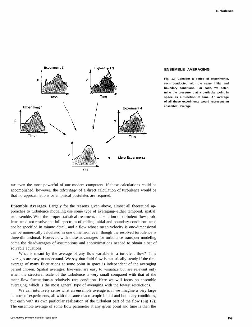
We can intuitively sense what an ensemble average is if we imagine a very largenumber of experiments, all with the same macroscopic initial and boundary conditions,but each with its own particular realization of the turbulent part of the flow (Fig 12).The ensemble average of some flow parameter at any given point and time is then the

ENSEMBLE AVERAGING

Fig. 12. Consider a series of experiments,

each conducted with the same initial and

boundary conditions. For each, we deter-

mine the pressure p at a particular point in

space as a function of time. An average

of all these experiments would represent an

ensemble average.


Reynolds-Stress Transport Equation. One of these fluctuational products, theReynolds stress tensor, is especially important; it is defined by

and

Then we take the ensemble average of these equations (commuting averages andderivatives where necessary and remembering that the average of a single fluctuatingvariable is zero) and obtain the mean-flow equations:

and

(13)


Turbulence

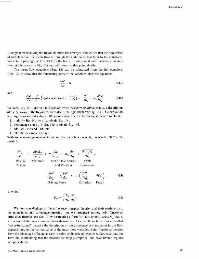
A single term involving the Reynolds stress has emerged, and we see that the only effectof turbulence on the mean flow is through the addition of that term to the equations.We note in passing that Eqs. 13 form the basis of point-functional turbulence models(the middle branch in Fig. 11) and will return to this point shortly.

The mean-flow equations (Eqs. 13) can be subtracted from the full equations(Eqs. 12) to show that the fluctuating parts of the variables obey the equations

(14a)

Rate ofChange

Advection Mean-Flow Source Tripleand Rotation Correlation

Driving Force

in which

Diffusion Decay

(16)

a function of the mean-flow variables themselves. As a result, such theories are called“point-functional” because the description of the turbulence at some point in the flowdepends only on the current value of the mean-flow variables. Point-functional theorieshave the advantage of being as easy to solve as the original Navier-Stokes equations buthave the shortcoming that the theories are largely empirical and have limited regionsof applicability.


Turbulence

TURBULENCE TRANSPORT

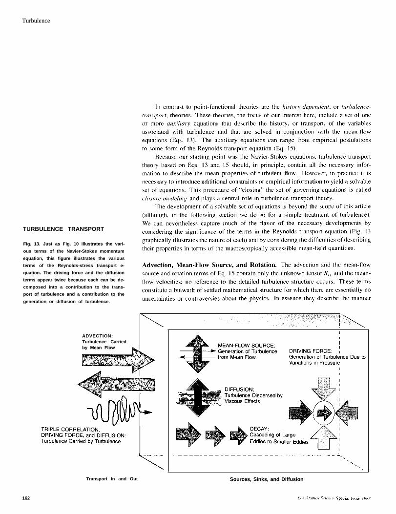
Fig. 13. Just as Fig. 10 illustrates the vari-

ous terms of the Navier-Stokes momentum

equation, this figure illustrates the various

terms of the Reynolds-stress transport e-

quation. The driving force and the diffusion

terms appear twice because each can be de-

composed into a contribution to the trans-

port of turbulence and a contribution to the

generation or diffusion of turbulence.

ADVECTION:Turbulence Carriedby Mean Flow

Transport In and Out

162

Sources, Sinks, and Diffusion

Turbulence

in which the mean flow moves turbulence from one place to another by translation,rotation, and stretching or contraction of the fluid.

(17)

Decomposing the variables into mean and fluctuating parts and taking the ensembleaverage (as we did before with Eqs. 12 and 13), we find that

(18)

The proportionality constant is a function of the turbulence intensity; indeed, moredetailed considerations indicate that

in which s is the length scale of the turbulence. It follows that

(20)

(21)

In this manner, we see what is meant by closure modeling, that is, the eliminationof any residual reference to details of the turbulence. For our purposes we need notdelve any deeper into this aspect of turbulence modeling; the example is sufficient toindicate some of the heuristic and empirical procedures we inevitably have been forcedto employ.

Driving Force. The pressure-velocity correlation terms (the first two terms on the rightside of Eq. 15) are especially important to the transport modeling of turbulence. Theydescribe one of the principal driving forces by which mean-flow energy finds its way


Turbulence

(22)

Diffusion and Decay. Of the last two terms in Eq. 15, the first is usually negligibleand represents diffusion of turbulence by molecular viscosity, which requires no furthermodeling. The second involves the tensor D i,, for which the usual procedure hasbeen to derive a horrendously complicated transport equation and attempt to solve thissimultaneously with the Reynolds transport equation. Such a procedure introduces ahost of additional correlation terms to be modeled, and much appeal to “intuition” isinvoked in the process.

Bypassing the fascinating but tedious discussion of these derivations, we cannevertheless describe several interesting properties of this second term. First, itscontraction

(23)


Turbulence

the eddies, which decay first by cascading to smaller eddies before converting to thermalenergy (Fig. 9). Thus, an alternative to the usual modeling of the behavior of D ij hasrecently emerged. We can get the same results by treating the decay of the large-scaleeddies as the energy source of the small-scale eddies. For this purpose the large-scale eddies are momentarily thought of as being “mean flow.” In some complicatingcircumstances, such as interpenetration of particles, this alternative modeling techniquehas proven so far to be the only tractable approach.

Simpler Transport Models and Examples of Their Application

Some problems do not warrant the degree of complexity and closure approximationrequired to numerically solve the full Reynolds-stress transport equation. A more con-ventional and practical approach uses the following approximation (called Boussinesq’sapproximation) for turbulence stresses in an incompressible fluid:

(24)

intois

(25)

(26)


Turbulence

Reynolds NumberRevisited

(1)

166

Turbulence

of thiskinetickinetic

167

Turbulence

THREE SIMPLIFIED

TURBULENCE CALCULATIONS

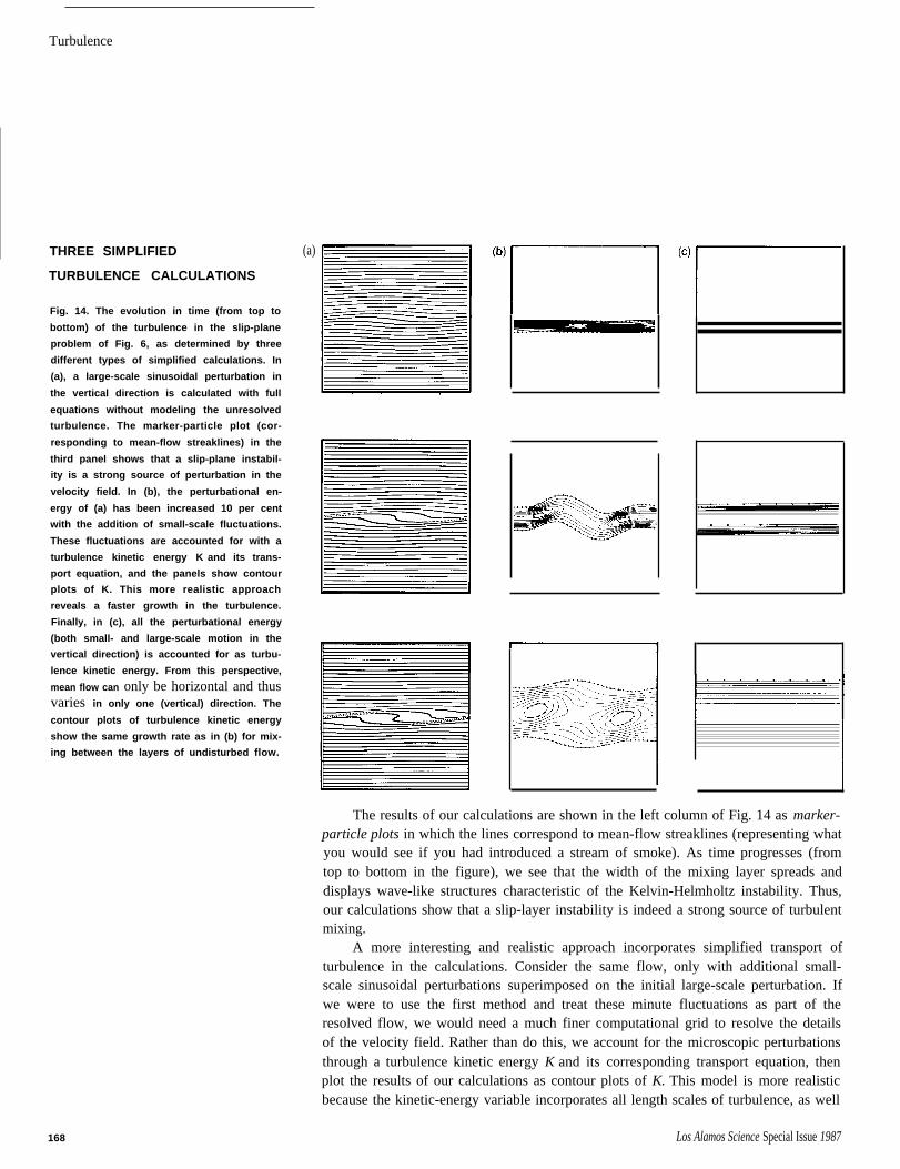
Fig. 14. The evolution in time (from top to

bottom) of the turbulence in the slip-plane

problem of Fig. 6, as determined by three

different types of simplified calculations. In

(a), a large-scale sinusoidal perturbation in

the vertical direction is calculated with full

equations without modeling the unresolved

turbulence. The marker-particle plot (cor-

responding to mean-flow streaklines) in the

third panel shows that a slip-plane instabil-

ity is a strong source of perturbation in the

velocity field. In (b), the perturbational en-

ergy of (a) has been increased 10 per cent

with the addition of small-scale fluctuations.

These fluctuations are accounted for with a

turbulence kinetic energy K and its trans-

port equation, and the panels show contour

plots of K. This more realistic approach

reveals a faster growth in the turbulence.

Finally, in (c), all the perturbational energy

(both small- and large-scale motion in the

vertical direction) is accounted for as turbu-

lence kinetic energy. From this perspective,

mean flow can only be horizontal and thusvaries in only one (vertical) direction. The

contour plots of turbulence kinetic energy

show the same growth rate as in (b) for mix-

ing between the layers of undisturbed flow.

168

(a)

The results of our calculations are shown in the left column of Fig. 14 as marker-particle plots in which the lines correspond to mean-flow streaklines (representing whatyou would see if you had introduced a stream of smoke). As time progresses (fromtop to bottom in the figure), we see that the width of the mixing layer spreads anddisplays wave-like structures characteristic of the Kelvin-Helmholtz instability. Thus,our calculations show that a slip-layer instability is indeed a strong source of turbulentmixing.

A more interesting and realistic approach incorporates simplified transport ofturbulence in the calculations. Consider the same flow, only with additional small-scale sinusoidal perturbations superimposed on the initial large-scale perturbation. Ifwe were to use the first method and treat these minute fluctuations as part of theresolved flow, we would need a much finer computational grid to resolve the detailsof the velocity field. Rather than do this, we account for the microscopic perturbationsthrough a turbulence kinetic energy K and its corresponding transport equation, thenplot the results of our calculations as contour plots of K. This model is more realisticbecause the kinetic-energy variable incorporates all length scales of turbulence, as well


Turbulence

Current Research

So far we have concentrated on turbulence in a single incompressible fluid withdensity perfectly constant in position and time (the downward branches of Fig. 11).Recently, our research has included additional features that are of interest to many ofthe new scientific and engineering directions at Los Alamos and other laboratories.These features are

. Two-phase flow interactions: the sources, sinks, and effects of turbulence in a fluid

containing particles, droplets, or bubbles of another material.● Density gradients: turbulence in an incompressible fluid for which variations of

temperature or the presence of some dissolved substance cause large variations indensity.

● Supersonic turbulence: the effects of high-speed processes on turbulence.In all cases, we continue to use the basic philosophy of transport modeling, which,despite some obvious difficulties, seems at present to be by far the most promisingapproach for the solution of practical problems.

Two-Phase Flow. Particles, drops, or bubbles suspended in a fluid-whether that fluidis a liquid or a gas-can significantly alter the turbulence and its effects. Intuitively,

Los Alamos .Science Special Issue 1987 169

Turbulence

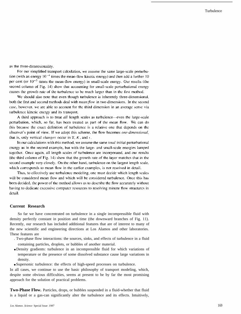
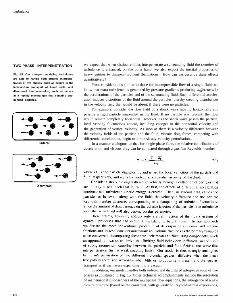
TWO-PHASE INTERPENETRATION

Fig. 15. Our transport modeling techniques

are able to handle both ordered interpene-

tration of two phases, such as occurs in the

laminar-flow transport of blood cells, and

disordered interpenetration, such as occurs

in a rapidly moving gas that contains sus-

pended particles.

we expect that when distinct entities interpenetrate a surrounding fluid the creation ofturbulence is enhanced; on the other hand, we also expect the inertial properties ofheavy entities to dampen turbulent fluctuations. How can we describe these effectsquantitatively?

From considerations similar to those for incompressible flow of a single fluid, weknow that extra turbulence is generated by pressure gradients producing differences inthe accelerations of the particles and of the surrounding fluid. Such differential acceler-ation induces distortions of the fluid around the particles, thereby creating disturbancesin the velocity field that would be absent if there were no particles.

For example, consider the flow field of a shock wave moving horizontally andpassing a rigid particle suspended in the fluid. If no particle was present, the flowwould remain completely horizontal. However, as the shock wave passes the particle,local velocity fluctuations appear, including changes in the horizontal velocity andthe generation of vertical velocity. As soon as there is a velocity difference betweenthe velocity fields of the particle and the fluid, viscous drag forces, competing withdifferential acceleration, begin to diminish any velocity perturbations.

In a manner analogous to that for single-phase flow, the relative contributions ofacceleration and viscous drag can be compared through a particle Reynolds number

transport as if each were expanding into a vacuum.In addition, our model handles both ordered and disordered interpenetration of two

phases as illustrated in Fig. 15. Other technical accomplishments include the resolutionof mathematical ill-posedness of the multiphase flow equations, the emergence of a newclosure principle (based on the constraint, with generalized Reynolds-stress expressions,

170 Los Alamos Science Special Issue /987

Turbulence

of exactly neutral stability for the mean-flow equations), and the development ofpractical modeling equations.

The modeling of turbulent flow with dispersed particles, droplets, or bubbles isof interest to a wide variety of scientific projects at the Laboratory. For example, to

model the transport of dust and debris by volcanic eruptions, one must concentrateon the interactions between particulate and hot-gas flows. To improve the design ofinternal combustion engines, one needs an accurate prediction of both the combustionefficiency and the spatial distribution of heat generation, which, in turn, requiresknowing the details of the mixing of fuel droplets and air. Although flow withinthe body’s circulatory system is normally not turbulent, the transport of blood cellscan be analyzed by using the equations for ordered two-field interpenetration. Otherapplications include modeling of the flow within nuclear reactors and the analysis ofshock-wave motion in a gas that contains suspended particles.

Density Gradients. The second area we are currently striving to understand withtransport modeling is turbulent mixing generated by strong density gradients that aresustained by large variations in thermal or material composition. Coupled with pressuregradients, such density gradients can lead to strongly contorted flow with intensevorticity near the steepest density variations. Again, the proper basis for deriving ageneralized Reynolds stress lies in decomposing the momentum rather than the velocity.

Among the most important configurations to be studied are those for which adjacentmaterials—initially quiescent and of very different densities—are rapidly acceleratedby a strong pressure gradient or heated by a sudden influx of radiation. The ensuingfluid instability (Richtmyer-Meshkov if the shock is going from heavy to light material,Rayleigh-Taylor for the opposite case (Fig. 7)) can act as a strong source for theturbulent mixing of the two materials.

For example, consider an experiment in which a plane shock wave progressesdown a closed cylindrical tube divided into two sections by a permeable membranewith air in the first section and helium in the second. As the shock passes from thedense to the less-dense gas, the air-helium interface is accelerated. Later, the interfaceis repeatedly decelerated by reflections from the rigid wall at the end of the tube.Interface instabilities lead to turbulent mixing of the two gases, and the initially sharpplane separating the gases becomes smeared and indistinct. Our work allows predictionof the average concentration across any strip of fluid taken normal to the nominalstreaming direction and calculation of velocity and density profiles within the turbulentmixing zone.

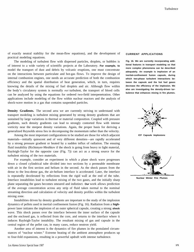
Instabilities driven by density gradients are important to the study of the implosiondynamics of pellets used in inertial confinement fusion (Fig. 16). Radiation from a high-power laser initiates the implosion of an outer spherical capsule, creating a strong shock

wave. This shock passes over the interface between the inner surface of the capsuleand the enclosed gas, is reflected from the core, and returns to the interface where itinduces Rayleigh-Taylor instability. The resultant mixing of gas and capsule in thecentral region of the pellet can, in many cases, reduce neutron yield.

Another area of interest is the dynamics of fire plumes in the postulated circum-stances of “nuclear winter.” Extreme heating of the ambient atmosphere produces upto four-fold expansions, resulting in a powerful updraft with intense turbulence.


CURRENT APPLICATIONS

Fig. 16. We are currently incorporating addi-

tional features in transport modeling so that

more complex phenomena can be described

adequately. An example is implosion of an

inertial-confinement fusion capsule, during

which two-phase turbulent interactions be-

tween the capsule and the hot fuel gases

decrease the efficiency of the implosion. We

also are investigating the density-driven tur-

bulence that enhances mixing in fire plumes.

ICF Capsule Implosions

Nuclear Winter Fire Plumes

171

Turbulence

Supersonic Turbulence. Mach-number effects often can be ignored, but, in somecases (such as the high-Mach-number mitigation of a Kelvin-Helmholtz instability),such effects are significant. Thus, a third feature of our recent work has been to in-clude the principal phenomena resulting from supersonic flow speeds. These effectsarise across shock waves, in the shear layers behind Mach-reflection triple-shock inter-sections, and in the shear layers behind shock waves normal to a deformable wall.

An unexpected result of our work is the discovery that laminar instability theory(as sketched out in the section entitled “Turbulence Energy: Sources and Sinks”) isapplicable to the study of supersonic turbulence. Despite the seeming inconsistency,this theory is providing highly relevant guidance to our early modeling efforts.

Concluding Remarks

A pertinent question is: What good is all this? Not only has our discussionillustrated several ways in which turbulence transport theory is heuristic or empirical,but the current large inventory of undetermined “universal” dimensionless parametersin its formulation is disturbing. Moreover, full expression of the theory is long andcomplicated, involving numerous coupled nonlinear partial differential equations. As aresult, a transport calculation requires either costly numerical solutions or questionableapproximations, or both.

What are the alternatives? There is no way to resolve turbulence in sufficientdetail for numerical calculations based on turbulence transport theory to representthe effects of any but the simplest circumstances. Mixing-length theories and otherpoint-functional approaches are hopelessly limited in their applicability. Fundamentalapproaches purporting to describe turbulence without empiricism are, in general, alsorestricted to highly idealized circumstances. Yet we are faced with the task of solvingan endless variety of fluid-flow problems, a large fraction of which include significantturbulence effects. We need to supply answers to old questions and guidance for newdevelopments in a meaningful way. At present, there seems to be no better approachto these challenging analytical tasks than that provided by turbulence transport theory.

Despite the shadows cast by these comments, the situation is actually far fromgloomy. Turbulence transport theory seems to be functioning far better than we haveany right to expect. There are at least four reasons for this good performance.

First, complex processes of nature often display a near universality in the collectiveeffects that are of most interest. Just as gas molecules almost always have a nearlyMaxwell-Boltzmann velocity distribution, it appears that turbulence tends toward asimilar universality in its stochastic structure. The success of the few-variable (orcollective, or moment) approach to turbulence modeling relies strongly on the validityof this contention. Although the extent to which universal behavior underlies most of therandom processes of nature is currently a matter of intense scientific and philosophicaldiscussion, much evidence supports the ubiquitous nature of this property. Perhaps,eventually, such universalities will help to successfully model such diverse instancesas thoughts in a brain, activities of groups of organisms (such as mobs of people), andthe dynamics of galaxies.

Next, turbulence transport modeling pays close attention to the binding constraintsof real physics: conservation of mass, momentum, and energy, as well as rotational and

172

Turbulence

translational invariance. Such modeling also accounts for history-dependent variationslacking in many other turbulence theories.

We have also paid great care to physically meaningful closure modeling. Auxiliaryderivations (like those of laminar instability analysis) combine with new formulationsof mathematical restrictions (like that of precisely neutral mean-flow stability in thepresence of generalized Reynolds-stress terms) to constrain our modeling proceduresin the most physically meaningful manner possible at each stage of the development.

Finally, investigators throughout the world have made numerous comparisonswith experiments, leading to corrections, improvements, and ultimately to considerableconfidence in the broad applicability of the results.

Future research will concentrate on several significant aspects of the theory. Clo-sure modeling, of course, continually needs strengthening, especially by first-principletechniques that decrease our reliance on empiricism. The numerical techniques needgreater stability, accuracy, and efficiency for a host of larger and more complicatedproblems.

But the most intriguing challenge is how to incorporate new and different physicalprocesses into our theories. For example, with dispersed-entity flow, we have scarcelybegun to understand the effects of a spectrum of entity sizes or the deformation ofindividual entities (including their fragmentation and coalescence) or the modificationsthat arise when the entities become close-packed (as they do, for example, duringdeposition and scouring of river-bed sand). The dispersal of turbulence energy throughacoustic or electromagnetic radiation is another interesting topic that needs considerabledevelopment. Deriving, testing, and applying the appropriate models will keep manyinvestigators busy for a long time. ■

Further Reading

B. J. Daly and F. H, Harlow. 1970. Transport equations in turbulence. Physics of Fluids 13: 2634–2649

B. E. Launder and D. B. Spalding, 1974. The numerical computation of turbulent flows. Computer Methodsin Applied Mechanics and Engineering 3: 269–289.

C. J. Chen and C. P, Nikitopoulos. 1979. On the near field characteristics of axisymmetric turbulent buoyantjets in a uniform environment. International Journal of Heat and Mass Transfer 22: 245–255.

D. Besnard and F. H. Harlow, 1985, Turbulence in two-field incompressible flow. Los Alamos NationalLaboratory report LA-10187–MS.

F. H. Harlow, D. L. Sandoval, and H, M. Ruppel. 1986. Mathematical modeling of biological ensembles.Los Alamos National Laboratory report LA–10765–MS.

D. Besnard, F. H. Harlow, and R. M. Rauenzahn. 1987. Conservation and transport properties of turbulencewith large density gradients. Los Alamos National Laboratory report LA–10911–MS,

D. Besnard and F, H. Harlow. Turbulence in multiphase flow. Submitted for publication in InternationalJournal of Multiphase Flow.


Turbulence

Authors

Didier Besnard is a frequent visitor to Los Alamosfrom the Commissariats a l’Energie Atomiquc inFrance. He is the recipient of several advanceddegrees in the fields of applied mathematics andengineering and has been employed since 1979 atthe Centre d’Etudes de Limeil-Valenton, near Paris,where he is head of the Groupe Interaction et Turbu-lence. He is especially active in the analytical andnumerical solution of problems in plasma physicsand the high-speed dynamics of compressible mate-rials. At Los Alamos he has worked in the Centerfor Nonlinear Studies and been a Visiting Scientistin the Theoretical Fluid Dynamics Group, collab-orating in the development of turbulence transporttheories, especially for multiphase flows and fluidswith large density variations. An avid rock climber,hiker, and skier, he enjoys frequent excursions tothe backwoods areas of both New Mexico and theFrench Alps. His wife, Anne, and daughter, Gaelle,join him in being a truly international family, spend-ing at least a month in New Mexico each summer.

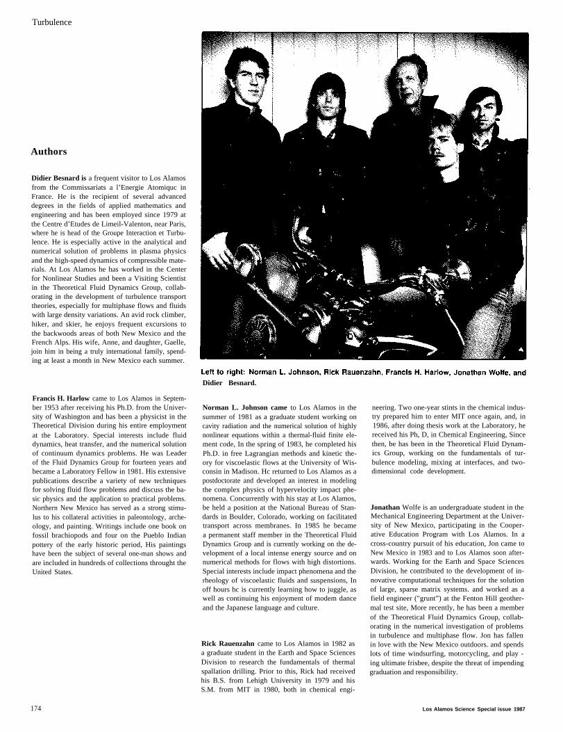
Didier Besnard.

Francis H. Harlow came to Los Alamos in Septem-ber 1953 after receiving his Ph.D. from the Univer-sity of Washington and has been a physicist in theTheoretical Division during his entire employmentat the Laboratory. Special interests include fluiddynamics, heat transfer, and the numerical solutionof continuum dynamics problems. He was Leaderof the Fluid Dynamics Group for fourteen years andbecame a Laboratory Fellow in 1981. His extensivepublications describe a variety of new techniquesfor solving fluid flow problems and discuss the ba-sic physics and the application to practical problems.Northern New Mexico has served as a strong stimu-lus to his collateral activities in paleontology, arche-ology, and painting. Writings include one book onfossil brachiopods and four on the Pueblo Indianpottery of the early historic period, His paintingshave been the subject of several one-man shows andare included in hundreds of collections throught theUnited States.

Norman L. Johnson came to Los Alamos in thesummer of 1981 as a graduate student working oncavity radiation and the numerical solution of highlynonlinear equations within a thermal-fluid finite ele-ment code, In the spring of 1983, he completed hisPh.D. in free Lagrangian methods and kinetic the-ory for viscoelastic flows at the University of Wis-consin in Madison. Hc returned to Los Alamos as apostdoctorate and developed an interest in modelingthe complex physics of hypervelocity impact phe-nomena. Concurrently with his stay at Los Alamos,be held a position at the National Bureau of Stan-dards in Boulder, Colorado, working on facilitatedtransport across membranes. In 1985 he becamea permanent staff member in the Theoretical FluidDynamics Group and is currently working on the de-velopment of a local intense energy source and onnumerical methods for flows with high distortions.Special interests include impact phenomena and therheology of viscoelastic fluids and suspensions, Inoff hours hc is currently learning how to juggle, aswell as continuing his enjoyment of modem danceand the Japanese language and culture.

Rick Rauenzahn came to Los Alamos in 1982 asa graduate student in the Earth and Space SciencesDivision to research the fundamentals of thermalspallation drilling. Prior to this, Rick had receivedhis B.S. from Lehigh University in 1979 and hisS.M. from MIT in 1980, both in chemical engi-

neering. Two one-year stints in the chemical indus-try prepared him to enter MIT once again, and, in1986, after doing thesis work at the Laboratory, hereceived his Ph, D, in Chemical Engineering, Sincethen, be has been in the Theoretical Fluid Dynam-ics Group, working on the fundamentals of tur-bulence modeling, mixing at interfaces, and two-dimensional code development.

Jonathan Wolfe is an undergraduate student in theMechanical Engineering Department at the Univer-sity of New Mexico, participating in the Cooper-ative Education Program with Los Alamos. In across-country pursuit of his education, Jon came toNew Mexico in 1983 and to Los Alamos soon after-wards. Working for the Earth and Space SciencesDivision, he contributed to the development of in-novative computational techniques for the solutionof large, sparse matrix systems. and worked as afield engineer ("grunt”) at the Fenton Hill geother-mal test site, More recently, he has been a memberof the Theoretical Fluid Dynamics Group, collab-orating in the numerical investigation of problemsin turbulence and multiphase flow. Jon has fallenin love with the New Mexico outdoors. and spendslots of time windsurfing, motorcycling, and play -ing ultimate frisbee, despite the threat of impendinggraduation and responsibility.

174 Los Alamos Science Special issue 1987

Documents

by Didier Besnard, Francis H. Harlow, Rick Rauenzahn, · by Didier Besnard, w hen the interface between two materials experiences strong accelerative Francis H. Harlow, or shearing