Embed Size (px)
Citation preview
Brigham Young University Brigham Young University
BYU ScholarsArchive BYU ScholarsArchive
Theses and Dissertations
2020-06-05
BYU Diesel Engine Lab Setup and Parasitic Losses of the Water BYU Diesel Engine Lab Setup and Parasitic Losses of the Water
Pump and Vacuum Pump on a Cummins 2.8L Engine Pump and Vacuum Pump on a Cummins 2.8L Engine
Eric Ashton Jessup Brigham Young University
Follow this and additional works at: https://scholarsarchive.byu.edu/etd
Part of the Engineering Commons
BYU ScholarsArchive Citation BYU ScholarsArchive Citation Jessup, Eric Ashton, "BYU Diesel Engine Lab Setup and Parasitic Losses of the Water Pump and Vacuum Pump on a Cummins 2.8L Engine" (2020). Theses and Dissertations. 8446. https://scholarsarchive.byu.edu/etd/8446
This Thesis is brought to you for free and open access by BYU ScholarsArchive. It has been accepted for inclusion in Theses and Dissertations by an authorized administrator of BYU ScholarsArchive. For more information, please contact [email protected], [email protected].
BYU Diesel Engine Lab Setup and Parasitic Losses of the Water Pump
and Vacuum Pump on a Cummins 2.8 L Engine
Eric Ashton Jessup
A thesis submitted to the faculty of Brigham Young University
in partial fulfillment of the requirements for the degree of
Master of Science
Dale R. Tree, Chair Bradley R. Adams Brian D. Iverson
Department of Mechanical Engineering
Brigham Young University
Copyright © 2020 Eric Ashton Jessup
All Rights Reserved
ABSTRACT
BYU Diesel Engine Lab Setup and Parasitic Losses of the Water Pump and Vacuum Pump on a Cummins 2.8 L Engine
Eric Ashton Jessup
Department of Mechanical Engineering, BYU Master of Science
The need to minimize carbon dioxide (CO2) emissions is becoming increasingly important with the total number of vehicles throughout the world exceeding one billion. Carbon dioxide emissions can be reduced by improving vehicle fuel efficiency. While electric transportation is gaining popularity, most passenger vehicles are still powered by gasoline or diesel engines. The main objective of this work was to provide opportunities for studying and improving the fuel efficiency of internal combustion engines (ICE). This was achieved by 1) Designing, building and testing auxiliary systems necessary to run a Cummins 2.8 L engine in a an engine test cell; 2) Creating educational labs for the ICE class; and 3) Measuring the parasitic losses of the vacuum pump and water pump on the installed Cummins 2.8 L diesel engine. All auxiliary systems were completed at a hardware cost of $8100 and are rated to support an engine with the power output capacity of 233 kW (312 hp). The educational laboratories enable future engineers to measure and assess the efficiency of internal combustions engines. The parasitic losses of the vacuum pump and water pump were found to impact the relative brake fuel conversion efficiency by 1.3% and 1.5% respectively over the Federal Test Procedure (FTP) cycle.
Keywords: parasitic losses, water pump, vacuum pump, internal combustion engine (ICE)

ACKNOWLEDGEMENTS
I am very grateful for the opportunity that I have had to pursue a master’s degree in
mechanical engineering from Brigham Young University. My experience has been filled with
hands on research, real world design, and problem solving. I learned to think more critically,
understand fundamental principles, design experiments, and clearly express technical results in
writing. I feel more confident in my ability to make a difference in any engineering role I accept
upon graduation.
I am grateful for my graduate advisor Dr. Tree and for his continual guidance,
mentorship, and review of my work and documents. I am grateful for the support of my fellow
graduate students. Additionally, I am grateful for the help of Caleb Brown, who volunteered to
help me as a part of his physics capstone design project. I am also grateful for Kevin Cole, who
provided critical data acquisition support for testing. Finally, I am grateful for the projects lab,
which aided me in the design and manufacture of auxiliary engine system components.
iv
TABLE OF CONTENTS ABSTRACT .................................................................................................................................... ii
ACKNOWLEDGEMENTS ........................................................................................................... iii
TABLE OF CONTENTS ............................................................................................................... iv
LIST OF TABLES ........................................................................................................................ vii
LIST OF FIGURES ..................................................................................................................... viii
1 Introduction ............................................................................................................................... 1
2 Literature Review...................................................................................................................... 5
Measurements of Water Pump Parasitic Losses ................................................................. 6
Measurements of Vacuum Pump Parasitic Losses ............................................................. 8
Anticipated Contributions ................................................................................................... 9
3 Background ............................................................................................................................. 10
AC Dynamometer Capabilities ......................................................................................... 10
4 Methods................................................................................................................................... 14
Engine Auxiliary Facilities Design Method ..................................................................... 14
4.1.1 Design Constraints by the Room ......................................................................... 16
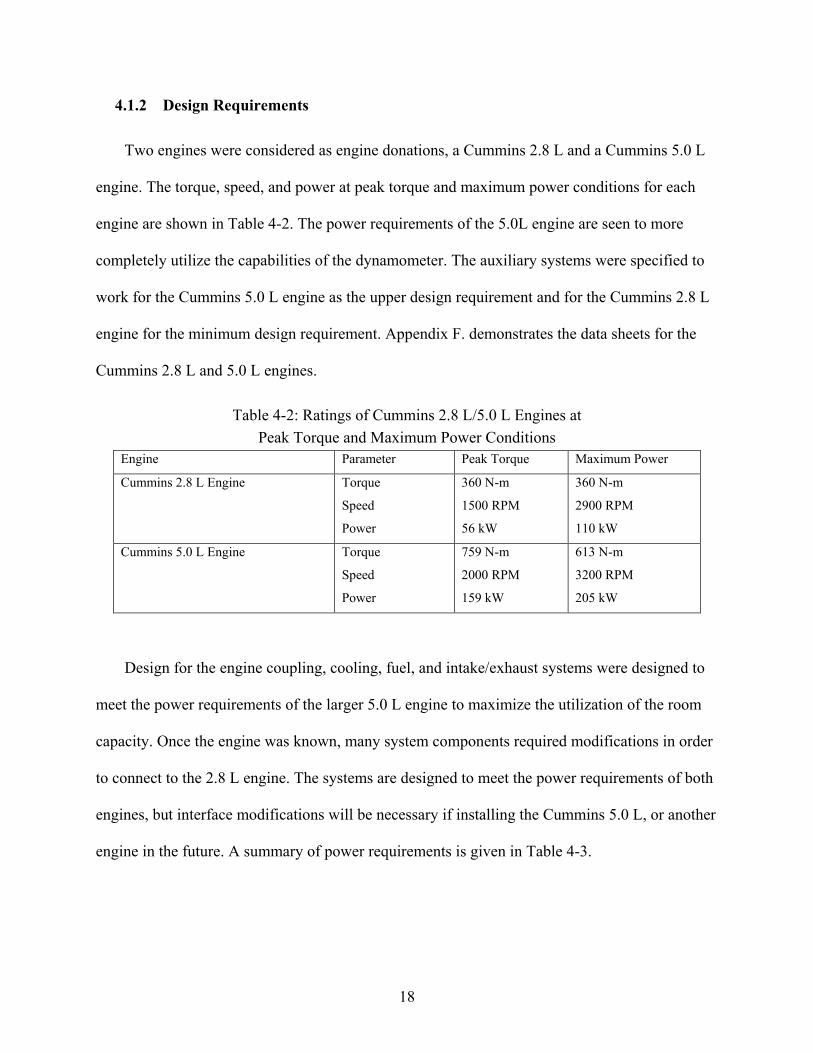
4.1.2 Design Requirements .......................................................................................... 18
4.1.3 Design Options, Analysis, and Selection ............................................................ 19
4.1.4 Final Options Selected ........................................................................................ 23
Lab Testing Methods ........................................................................................................ 24
Measuring Parasitic Losses of the Water Pump ............................................................... 24
Measuring Parasitic Losses of the Vacuum Pump ............................................................ 27
5 Results and Discussion ........................................................................................................... 30
Engine Lab Setup .............................................................................................................. 30
v
Driveline Coupling System ............................................................................................... 32
5.2.1 Driveline Coupling Description .......................................................................... 32
5.2.2 Driveline Coupling Rated Performance .............................................................. 35
5.2.3 Driveline Coupling Measured Performance ........................................................ 35
Coolant System ................................................................................................................. 35
5.3.1 Coolant System Description ................................................................................ 35
5.3.2 Coolant System Rated Performance .................................................................... 36
5.3.3 Coolant System Measured Performance ............................................................. 37
Intake/Exhaust System ...................................................................................................... 37
5.4.1 Intake/Exhaust System Description .................................................................... 37
5.4.2 Intake/Exhaust System Rated Performance ........................................................ 38
5.4.3 Intake/Exhaust System Measured Performance .................................................. 39
Fuel System ....................................................................................................................... 40
5.5.1 Fuel System Description ..................................................................................... 40
5.5.2 Fuel System Rated Performance ......................................................................... 41
5.5.3 Fuel System Measured Performance ................................................................... 42
Controls/DAQ System ...................................................................................................... 42
5.6.1 Controls/DAQ System Description ..................................................................... 42
5.6.2 Controls/DAQ System Rated Performance ......................................................... 43
5.6.3 Controls/DAQ System Measured Performance .................................................. 43
Summary of Engine Auxiliary Setup Ratings and Measured Performance ...................... 44
Example Coursework Engine Lab Testing ....................................................................... 47
Measuring Parasitic Losses of the Water Pump ............................................................... 50
vi
5.9.1 Open Thermostat ................................................................................................. 50
5.9.2 Closed Thermostat ............................................................................................... 57
Measuring Parasitic Losses of the Vacuum Pump ............................................................ 61
Combined Parasitic Losses ............................................................................................... 64
6 Summary and Conclusions ..................................................................................................... 73
Appendix A. Bill of Materials for Engine Setup .......................................................................... 76
Appendix B. Coupling Assembly Drawings ................................................................................. 82
Appendix C. Heat Exchanger Specifications and Drawing .......................................................... 93
Appendix D. Wiring Diagram for Controls/ Data Acquisition ..................................................... 95
Appendix E. Engine Lab Power Capacity Calculations ............................................................... 96
Appendix F. Data Sheets for Cummins 2.8 L and 5.0 L engines ................................................. 98
Appendix G. Diesel Engine Operating Instructions ................................................................... 102
Appendix H. Diesel Engine Laboratory Experiment Instructions and Sample Data .................. 105
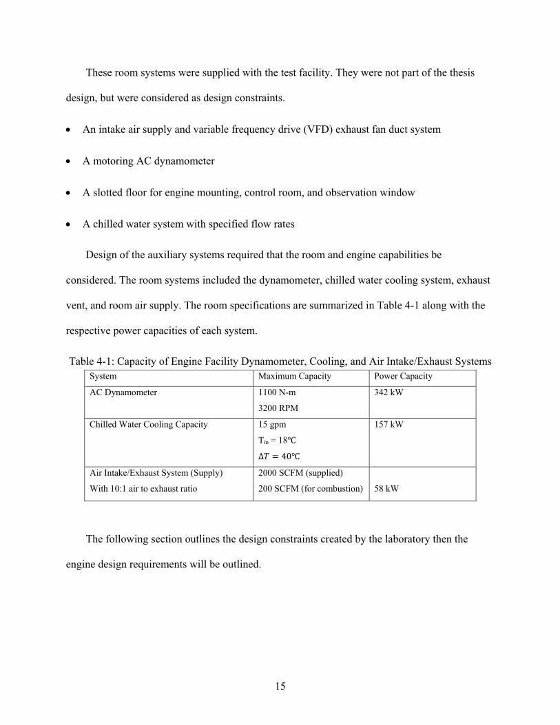
vii
LIST OF TABLES Table 4-1: Capacity of Engine Facility Dynamometer, Cooling, and Air Intake/Exhaust Systems
..................................................................................................................................... 15
Table 4-2: Ratings of Cummins 2.8 L/5.0 L Engines at ............................................................... 18
Table 4-3: Design Requirement Targets for Engine Auxiliary Systems ...................................... 19
Table 4-4: Coupling Options Considered ..................................................................................... 20
Table 4-5: Auxiliary Systems Selected Options ........................................................................... 23
Table 4-6: Specifications for Sensors Used to Test Parasitic Losses ........................................... 26
Table 4-7: Vacuum Pump Test Variations .................................................................................... 29
Table 5-1: Rated and Demonstrated Results for Key Component Parameters. ............................ 45
Table 5-2: Relative and absolute brake fuel conversion efficiency improvements possible for
various drive cycles by removing the vacuum and water pumps from the Cummins
2.8 L engine. ............................................................................................................... 71
Table A-1: Bill of Materials for Engine Coupling System ........................................................... 76
Table A-2: Bill of Materials for Engine Coolant System ............................................................. 77
Table A-3: Bill of Materials for Engine Intake and Exhaust System ........................................... 78
Table A-4: Bill of Materials for Engine Fuel System ................................................................... 79
Table A-5: Bill of Materials for Engine Controls and Data Acquisition System ......................... 80
Table A-6: Bill of Materials for Miscellaneous Lab Components ............................................... 81
viii
LIST OF FIGURES
Figure 1-1: Schematic showing how fuel energy is used, or lost, during combustion in an ICE
vehicle. .......................................................................................................................... 3
Figure 2-1: Methods used in the literature to measure water pump parasitic losses using pump
shaft torque.................................................................................................................... 7
Figure 4-1: Dyne Systems AC Dynamometer Torque and Power Curves ................................... 16
Figure 4-2: Diagram of the Water Pump Test Setup .................................................................... 25
Figure 4-3: Actual Water Pump Parasitic Loss Test Setup ........................................................... 27
Figure 4-4: Actual Vacuum Pump Parasitic Loss Test Setup ....................................................... 28
Figure 5-1: Schematic of Engine Test Cell Setup with Auxiliary Systems .................................. 31
Figure 5-2: Final Engine Lab Setup with Installed Auxiliary Systems ........................................ 32
Figure 5-3: Final Engine to Dynamometer Coupling Components .............................................. 33
Figure 5-4: Installed Engine to Dynamometer Coupling Assembly ............................................. 34
Figure 5-5: Installed Plate Heat Exchanger with Coolant Lines Labelled .................................... 36
Figure 5-6: Intake and Exhaust System Components ................................................................... 38
Figure 5-7: Installed Fuel System Components ............................................................................ 40
Figure 5-8: Left: Engine bay - Engine control unit and data acquisition system. Right: Control
room - dynamometer control box, computer with LabVIEW data recording software.
..................................................................................................................................... 43
Figure 5-9: Schematic of engine test cell set-up with rated power capacity limitations. ............. 46
Figure 5-10: Sample data set for brake torque as a function of fuel flow rate at a constant speed
of 1500 RPM. Error bars represent 1 standard deviation of 4 data points. ................. 47
ix
Figure 5-11: Sample data set for brake power as a function of fuel flow rate at a constant speed
of 1500 RPM. Error bars represent 1 standard deviation of 4 data points. ................. 48
Figure 5-12: Sample data set for brake fuel conversion efficiency as a function of fuel flow rate
at a constant speed of 1500 RPM. Error bars represent 1 standard deviation for 4 data
points. .......................................................................................................................... 49
Figure 5-13: Sample data set and rough trend lines for emissions concentrations as a function of
fuel flow for Cummins 2.8 L engine running at 1500 RPM. Error bars represent 1
standard deviation for 4 data points. ........................................................................... 50
Figure 5-14: Volume flow rate of the water pump as a function of engine speed for an open
thermostat condition.................................................................................................... 51
Figure 5-15: Pressure changes across water pump, engine, and return (radiator) for open
thermostat tests............................................................................................................ 52
Figure 5-16: Torque required by water pump shaft to pump water through open thermostat loop
as a function of water pump speed. ............................................................................. 54
Figure 5-17: Water pump power input and output for the open thermostat speed sweeps as a
function of water pump speed. .................................................................................... 55
Figure 5-18: Water pump efficiency as a function of water pump speed for the open thermostat
water pump speed sweeps. .......................................................................................... 56
Figure 5-19: Pressure changes across water pump, engine, and return (bypass) for closed
thermostat tests............................................................................................................ 57
Figure 5-20: Water pump shaft torque as a function of water pump speed for open and closed
thermostat test sweeps................................................................................................. 58
Figure 5-21: Correlation of volume flow rate as a function of pressure drop across the engine. . 59
x
Figure 5-22: Predicted volume flow rate as a function of water pump speed for the closed
thermostat. ................................................................................................................... 59
Figure 5-23: Water pump power input and output for the open and closed thermostat sweeps as a
function of water pump speed. Powers are for a ‘new’ engine and radiator with little
restrictions. Power requirements will be larger with more restrictions or fouling in
the engine. ................................................................................................................... 60
Figure 5-24: Water pump efficiency as a function of water pump speed for the open and closed
thermostat cases. ......................................................................................................... 61
Figure 5-25: Torque input required as a function of vacuum pump speed ................................... 62
Figure 5-26: Average torque required to power vacuum pump for various test cases. ................ 63
Figure 5-27: Vacuum pump power input as a function of vacuum pump speed. ......................... 63
Figure 5-28: Vacuum pressure as a function of time required to reduce the pressure in a 2 L
container open to atmosphere and closed. .................................................................. 64
Figure 5-29: Shaft torque required by the vacuum and water pumps as a function of engine
speed. .......................................................................................................................... 65
Figure 5-30: Shaft power required by the vacuum and water pumps as a function of engine
speed. .......................................................................................................................... 66
Figure 5-31: Percent of engine power consumed by the vacuum pump as a function of engine
speed. Different curves represent different engine fuel load conditions. ................... 67
Figure 5-32: Percent of engine power consumed by the water pump as a function of engine
speed. Different curves represent different engine fuel load conditions. ................... 68
xi
Figure 5-33: Engine power load for the FTP cycle and corresponding power consumption of the
water pump and vacuum pump. (Note that pump power is shown on a scale 10 times
smaller than engine power in order to display trends) ................................................ 70
Figure B1: Side View of Driveline Coupling Assembly .............................................................. 83
Figure B2: Dodge PH-131 Flexible Element Specifications ........................................................ 85
Figure B3: Drawing for Flywheel Modifications (SAE 11.5 Modified) ...................................... 86
Figure B4: MSI Shaft to Flange Adapter ...................................................................................... 87
Figure B5: Drawing of Driveline Shaft ........................................................................................ 88
Figure B6: Drawing of Front Motor Mounts ................................................................................ 89
Figure B7: Drawing of Rear Motor Mounts ................................................................................. 90
Figure B8: Drawing of Motor Mount Water Jet Pattern ............................................................... 91
Figure B9: Drawing for Driveline Guard ...................................................................................... 92
Figure C1: Specifications for TTS Heat Exchanger ..................................................................... 93
Figure C2: Drawing for TTS Heat Exchanger .............................................................................. 94
Figure D1: Wiring Diagram for Controls and Data Acquisition System...................................... 95
Figure E1: Cummins 2.8 L Data Sheet ......................................................................................... 99
Figure E2: Cummins 5.0 L Data Sheet ....................................................................................... 101
1
1 INTRODUCTION
Internal Combustion Engine (ICE) powered vehicles provide an inexpensive and convenient
mode of transportation for hundreds of millions of people in the United States. During
combustion, the gasoline or diesel fuel used to power an ICE reacts with air to release energy and
is converted into carbon dioxide (CO2) and water (H2O). Carbon dioxide is a greenhouse gas,
which is considered a contributor to global climate change and is therefore a global pollutant. If a
vehicle is more efficient, it uses less fuel, saves money, and emits less CO2 into the atmosphere.
In 2012, the Environmental Protection Agency, Department of Transportation, and
National Highway Traffic Safety Administrations issued regulations requiring automotive
manufacturers to meet emissions levels culminating in “an average industry fleet-wide level of
163 grams/mile of CO2 in model year 2025, which is equivalent to 54.5 miles per gallon (mpg)”
[1]. While these targets are currently under political and legal evaluation [2], [3], reduction of
CO2 emissions is clearly a national interest.
Engines are complex systems that have been under development for over a century. In order
for efficiency improvements to be made, engineers should seek to understand the fundamental
principles of operation and have opportunities to explore changes through experimental work.
BYU has the opportunity to contribute to future engine design and research through the use of a
new facility designed for internal combustion engine testing and research. The facility provided
2
space, an AC motoring dynamometer, a 2.8 L Cummins diesel engine, chilled water supply, air
supply, and exhaust fans. The facility provided an opportunity for several objectives.
The first objective was to design, fabricate and test the auxiliary systems necessary run the
Cummins engine in the test cell. Fulfillment of this objective required the design and installation
of the following engine auxiliary systems: 1) Engine coupling system, 2) Cooling system, 3)
Intake and Exhaust system, 4) Fuel system, 5) Controls and Data Acquisition system.
The second objective was to set up instructional laboratories for the internal combustion
engines (ICE) class. One lab was to demonstrate the brake fuel conversion efficiency of a diesel
engine at a constant speed and variable loads (fuel flow rates). A second lab was to demonstrate
the emissions of the engine for the same speed and loads. The understanding of the correlation
between fuel efficiency and emissions will enable current, and future, students to become
informed engineers that will make efficiency improvements in the future.
The third objective was to measure the parasitic losses of the water pump and vacuum pump
on the Cummins 2.8 L diesel engine. The water pump and vacuum pumps were selected for
parasitic loss testing in compliance to a request from Cummins, who donated the engine.
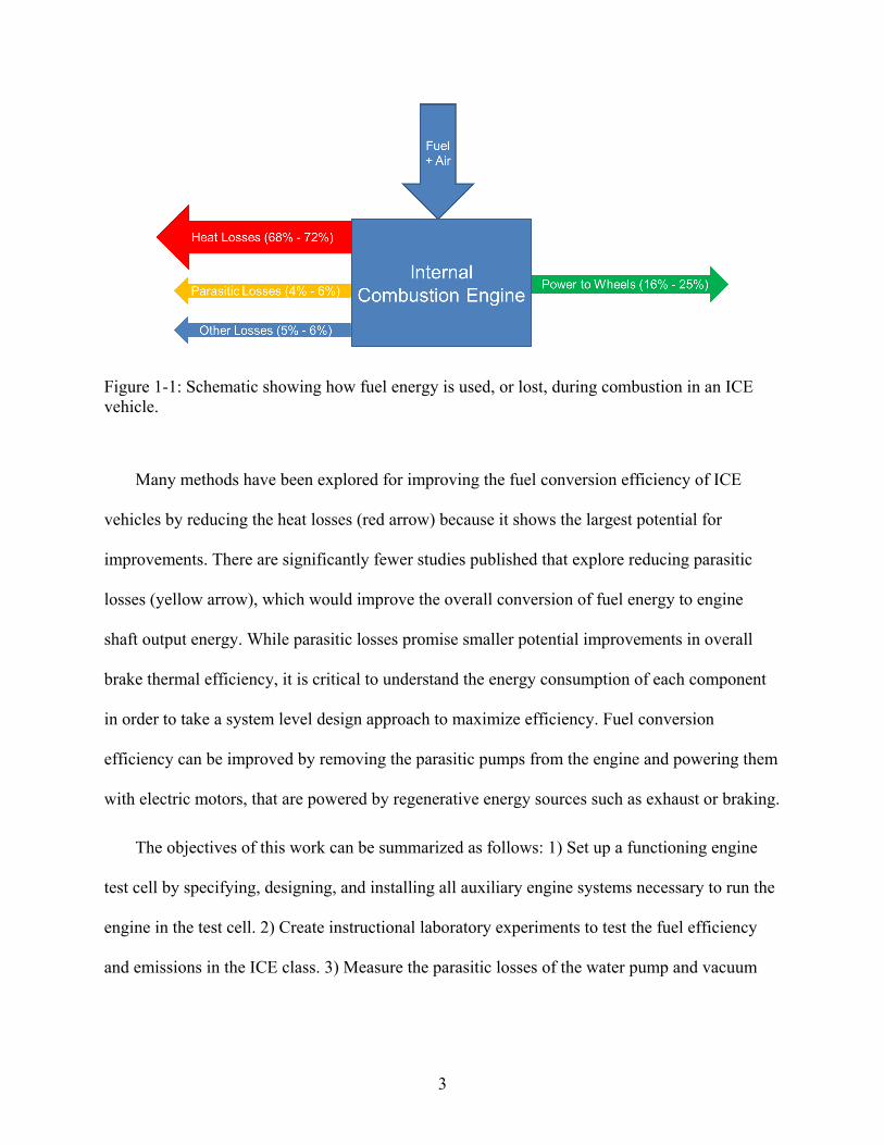
Figure 1-1 [4] is a schematic demonstrating how fuel energy is used in an internal
combustion engine. Fuel enters the engine (top arrow) and is combusted, 16% - 25% of that
energy is used to propel the vehicle forward (green arrow), while the rest of the energy is lost.
Most energy, 68% - 72%, (red arrow) is lost as heat. Other vehicle losses such as wind drag
remove 5% - 6% (blue arrow on left). The last 4% - 6% of the energy is considered parasitic
losses (yellow arrow). Parasitic losses consist of auxiliary pumps that remove energy from the
engine; examples of these are water pumps, vacuum pumps, oil pumps, and AC compressors.
3
Figure 1-1: Schematic showing how fuel energy is used, or lost, during combustion in an ICE vehicle.
Many methods have been explored for improving the fuel conversion efficiency of ICE
vehicles by reducing the heat losses (red arrow) because it shows the largest potential for
improvements. There are significantly fewer studies published that explore reducing parasitic
losses (yellow arrow), which would improve the overall conversion of fuel energy to engine
shaft output energy. While parasitic losses promise smaller potential improvements in overall
brake thermal efficiency, it is critical to understand the energy consumption of each component
in order to take a system level design approach to maximize efficiency. Fuel conversion
efficiency can be improved by removing the parasitic pumps from the engine and powering them
with electric motors, that are powered by regenerative energy sources such as exhaust or braking.
The objectives of this work can be summarized as follows: 1) Set up a functioning engine
test cell by specifying, designing, and installing all auxiliary engine systems necessary to run the
engine in the test cell. 2) Create instructional laboratory experiments to test the fuel efficiency
and emissions in the ICE class. 3) Measure the parasitic losses of the water pump and vacuum

4
pump on a Cummins 2.8 L diesel engine to determine the brake fuel conversion efficiency
improvement possible by removing the vacuum pump and water pump from the engine.
5
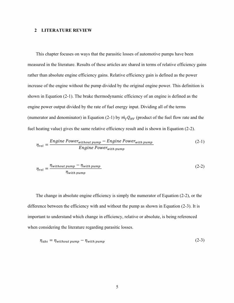
2 LITERATURE REVIEW
This chapter focuses on ways that the parasitic losses of automotive pumps have been
measured in the literature. Results of these articles are shared in terms of relative efficiency gains
rather than absolute engine efficiency gains. Relative efficiency gain is defined as the power
increase of the engine without the pump divided by the original engine power. This definition is
shown in Equation (2-1). The brake thermodynamic efficiency of an engine is defined as the
engine power output divided by the rate of fuel energy input. Dividing all of the terms
(numerator and denominator) in Equation (2-1) by 𝑚𝑚𝑓𝑓 𝑄𝑄𝐻𝐻𝐻𝐻 (product of the fuel flow rate and the
fuel heating value) gives the same relative efficiency result and is shown in Equation (2-2).
𝜂𝜂𝑟𝑟𝑟𝑟𝑟𝑟 =𝐸𝐸𝐸𝐸𝐸𝐸𝐸𝐸𝐸𝐸𝐸𝐸 𝑃𝑃𝑃𝑃𝑃𝑃𝐸𝐸𝑃𝑃𝑤𝑤𝑤𝑤𝑤𝑤ℎ𝑜𝑜𝑜𝑜𝑤𝑤 𝑝𝑝𝑜𝑜𝑝𝑝𝑝𝑝 − 𝐸𝐸𝐸𝐸𝐸𝐸𝐸𝐸𝐸𝐸𝐸𝐸 𝑃𝑃𝑃𝑃𝑃𝑃𝐸𝐸𝑃𝑃𝑤𝑤𝑤𝑤𝑤𝑤ℎ 𝑝𝑝𝑜𝑜𝑝𝑝𝑝𝑝
𝐸𝐸𝐸𝐸𝐸𝐸𝐸𝐸𝐸𝐸𝐸𝐸 𝑃𝑃𝑃𝑃𝑃𝑃𝐸𝐸𝑃𝑃𝑤𝑤𝑤𝑤𝑤𝑤ℎ 𝑝𝑝𝑜𝑜𝑝𝑝𝑝𝑝 (2-1)
𝜂𝜂𝑟𝑟𝑟𝑟𝑟𝑟 =𝜂𝜂𝑤𝑤𝑤𝑤𝑤𝑤ℎ𝑜𝑜𝑜𝑜𝑤𝑤 𝑝𝑝𝑜𝑜𝑝𝑝𝑝𝑝 − 𝜂𝜂𝑤𝑤𝑤𝑤𝑤𝑤ℎ 𝑝𝑝𝑜𝑜𝑝𝑝𝑝𝑝
𝜂𝜂𝑤𝑤𝑤𝑤𝑤𝑤ℎ 𝑝𝑝𝑜𝑜𝑝𝑝𝑝𝑝 (2-2)
The change in absolute engine efficiency is simply the numerator of Equation (2-2), or the
difference between the efficiency with and without the pump as shown in Equation (2-3). It is
important to understand which change in efficiency, relative or absolute, is being referenced
when considering the literature regarding parasitic losses.
𝜂𝜂𝑎𝑎𝑎𝑎𝑎𝑎 = 𝜂𝜂𝑤𝑤𝑤𝑤𝑤𝑤ℎ𝑜𝑜𝑜𝑜𝑤𝑤 𝑝𝑝𝑜𝑜𝑝𝑝𝑝𝑝 − 𝜂𝜂𝑤𝑤𝑤𝑤𝑤𝑤ℎ 𝑝𝑝𝑜𝑜𝑝𝑝𝑝𝑝 (2-3)
6
Measurements of Water Pump Parasitic Losses
The water pump moves coolant through the engine and the radiator to cool engine
components and prevent engine failure; it is normally run off of a belt and is a multiple of engine
speed regardless of how much pumping power is needed to cool the engine. There were six
studies found that measured parasitic losses associated with the water pump on an engine. One
measured the fuel consumption of a 2011 Mercedes Sprinter van with a 3.0 L V6 diesel engine
that was driven on a chassis dyno with a dual mode (electrical/mechanical) water pump; this
study showed a 2.3% relative fuel efficiency improvement [5]. Two additional studies
demonstrated the potential to improve fuel economy by 5% by electrifying the water pump and
cooling fan [6] [7]. However, one of these studies shows that 95.5% of this efficiency gain is
achieved by electrifying the cooling fan, while only 4.5% is attributed to electrifying the water
pump; this would equate to a 0.4% relative fuel efficiency improvement from the electric water
pump [6]. Another study measured the water pump parasitic losses on a 280kW diesel bus engine
to be 0.4% by measuring the torque and speed on the water pump shaft during the normal bus
drive cycle [8]. Finally, one paper demonstrated a method for measuring parasitic losses of the
water pump by driving the pump shaft with an external motor and measuring pump speed and
torque; this study shows a 0.3-1.3% relative brake thermal efficiency improvement for a 15 L
Cummins Engine [9].
The range of parasitic loss results displayed by these papers is large; obtaining more
parasitic loss data will help narrow down this wide range of results. Three of these papers used
methods of measuring fuel consumption or brake torque on a vehicle in order to quantify
parasitic losses [5] [6] [7]. The problem with this method is that parasitic losses are very small
7
compared to total engine output power. It is very difficult to accurately measure a small change
by measuring the difference between two relatively large numbers.
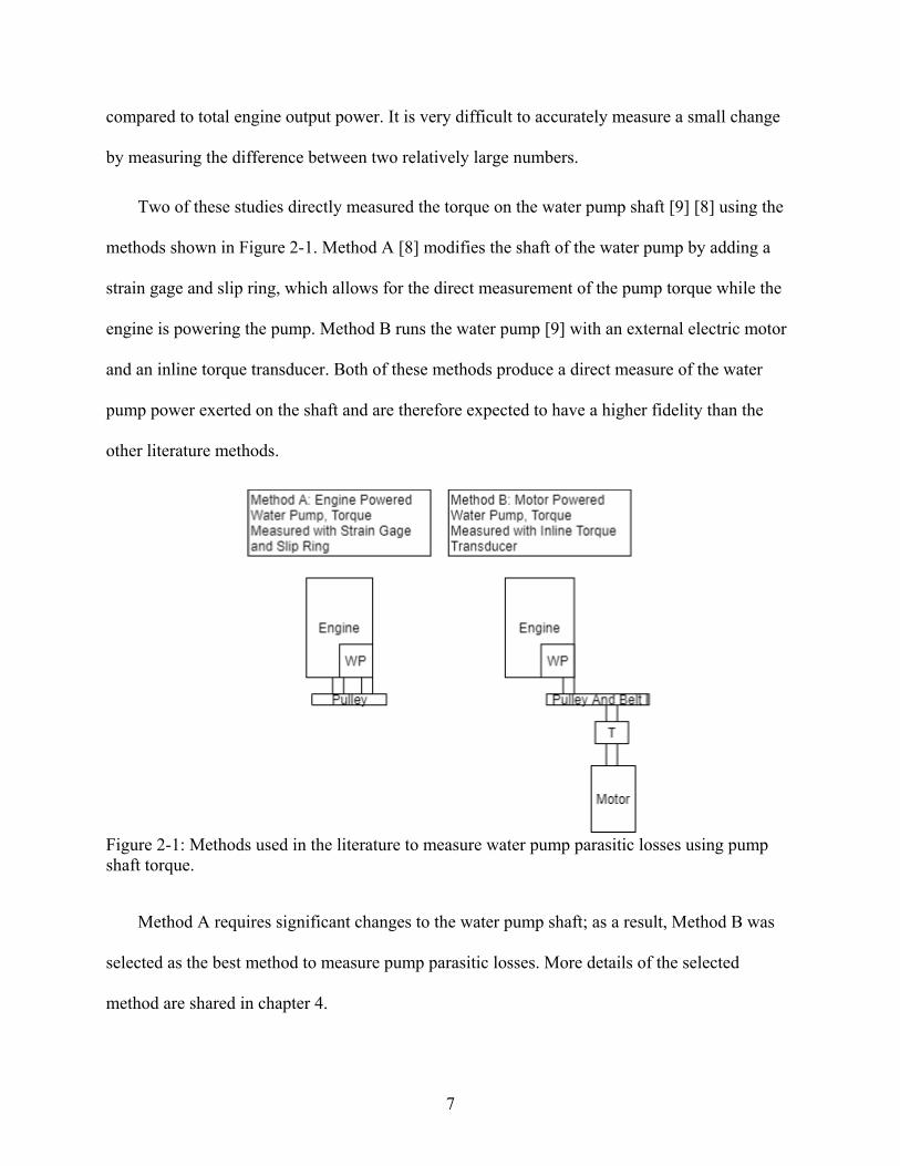
Two of these studies directly measured the torque on the water pump shaft [9] [8] using the
methods shown in Figure 2-1. Method A [8] modifies the shaft of the water pump by adding a
strain gage and slip ring, which allows for the direct measurement of the pump torque while the
engine is powering the pump. Method B runs the water pump [9] with an external electric motor
and an inline torque transducer. Both of these methods produce a direct measure of the water
pump power exerted on the shaft and are therefore expected to have a higher fidelity than the
other literature methods.
Figure 2-1: Methods used in the literature to measure water pump parasitic losses using pump shaft torque.
Method A requires significant changes to the water pump shaft; as a result, Method B was
selected as the best method to measure pump parasitic losses. More details of the selected
method are shared in chapter 4.
8
Findings from the six studies suggest that the parasitic losses of the water pump will be
between 0.4% – 2.3 % relative fuel efficiency improvement. It is important to note that a small
efficiency improvement (0.4% - 2.3%) holds the potential to save hundreds of millions of gallons
of fuel in the United States alone, if this improvement was applied to every vehicle. This simple
illustration shows why even a 1% improvement in fuel efficiency is of interest.
Measurements of Vacuum Pump Parasitic Losses
The vacuum pump supplies vacuum to a reservoir that is used to actuate the brakes on
vehicles and perform other functions; it is normally run off the camshaft at half the engine speed
regardless of how much vacuum is needed. Two studies were found that quantify the parasitic
power losses of a mechanical vacuum pump. One of these simply tested the fuel economy over a
typical drive cycle for a car and a larger utility vehicle respectively with a mechanical and
electric vacuum pump. The data were then generalized to a yearly distance of 20,000 km and
showed the potential to save 14 L of diesel fuel in a year. The results of this study showed a fuel
efficiency improvement with an electrified vacuum pump, but it did not quantify the total
parasitic load of the vacuum pump [10].
The second study removed the vacuum pump from the engine and powered it with an
electric motor as it filled a 10 L container with vacuum. The torque on the vacuum pump shaft
was measured with an inline torque transducer. These results showed the potential for a 1.5%
relative fuel efficiency improvement [11].
The lack of published research in this area suggests additional data could be impactful by
providing further quantification of vacuum pump parasitic losses.
9
Anticipated Contributions
The purpose of this thesis is to make a contribution in the area of fuel efficiency of internal
combustion engines. This purpose will be met in multiple ways.
The first objective is to set up an operational engine test lab (outfitted with all necessary
auxiliary systems), while not exceeding a hardware budget of $20,000. This lab will be capable
of being used for ICE class labs, capstone projects, and future research. Each of these uses will
provide students with a way to familiarize themselves with engine operation, efficiency, and
emissions. Education is a critical step for improving efficiency and reducing emissions in the
future.
The second objective is to create experimental labs for students in the ICE class to run and
learn about fuel efficiency and emissions of a diesel engine. Deliverables will include
instructions on how to run the engine and take data for the respective labs. This will further
enhance the ability of students to learn about ICEs.
The third and final objective is to measure the total parasitic losses of the water pump and
vacuum pump on the Cummins 2.8 L engine. The deliverable will be a report outlining these
findings. (See section 5.11) The parasitic losses of these pumps represent the total potential for
fuel efficiency improvements by removing the pumps from the engine and powering them with
regenerative energy sources. This testing will provide additional insights into parasitic losses as
few studies are publicly available. It also has the potential to provide automotive manufacturers
with key information needed to take a system level approach to improve vehicle fuel efficiency.
10
3 BACKGROUND
This chapter provides information useful for understanding how an AC dynamometer (an
apparatus used to test an engine) works when connected to an engine to achieve the torque,
speed, and power data that is required for the engine laboratory experiments.
AC Dynamometer Capabilities
Equation (3-1) shows the relationship between the forces acting on the engine crankshaft
from combustion, friction, and the dynamometer.
The first term on the left side is the power generated by the engine, ��𝑊𝑟𝑟𝑒𝑒𝑒𝑒, on the crankshaft.
The engine produces work in each cycle (two rotations) dependent on the amount of fuel injected
and burned. The work produced in a cycle and the torque produced on the connecting rod are
proportional and differ only by a constant. Thus, an operator may produce more work or torque
by increasing the amount of fuel injected per cycle up to the point that there is no longer enough
air to burn the fuel. At this point the engine is at 100% of its rated load. The pedal position can
represent the amount of fuel injected per cycle. When the engine is at idle, the pedal position is
somewhere near 5-10% of the full load or full pedal position. The engine power produced within
the cylinder is proportional to the product of the fuel injected per cycle (or work per cycle) and
engine speed (cycles/second) and is called the indicated power.
The second term in the equation, ��𝑊𝑓𝑓𝑟𝑟𝑤𝑤𝑓𝑓, represents the losses in power from the crankshaft
due to friction, pumps, compressors, and the alternator. These are termed parasitic losses or
friction power. The loss in a given cycle tends to be proportional to engine speed. As engine
speed increases, the friction loss per cycle increases. The friction power is the product of the
11
engine speed and the friction work per cycle and is therefore proportional to the engine speed
squared.
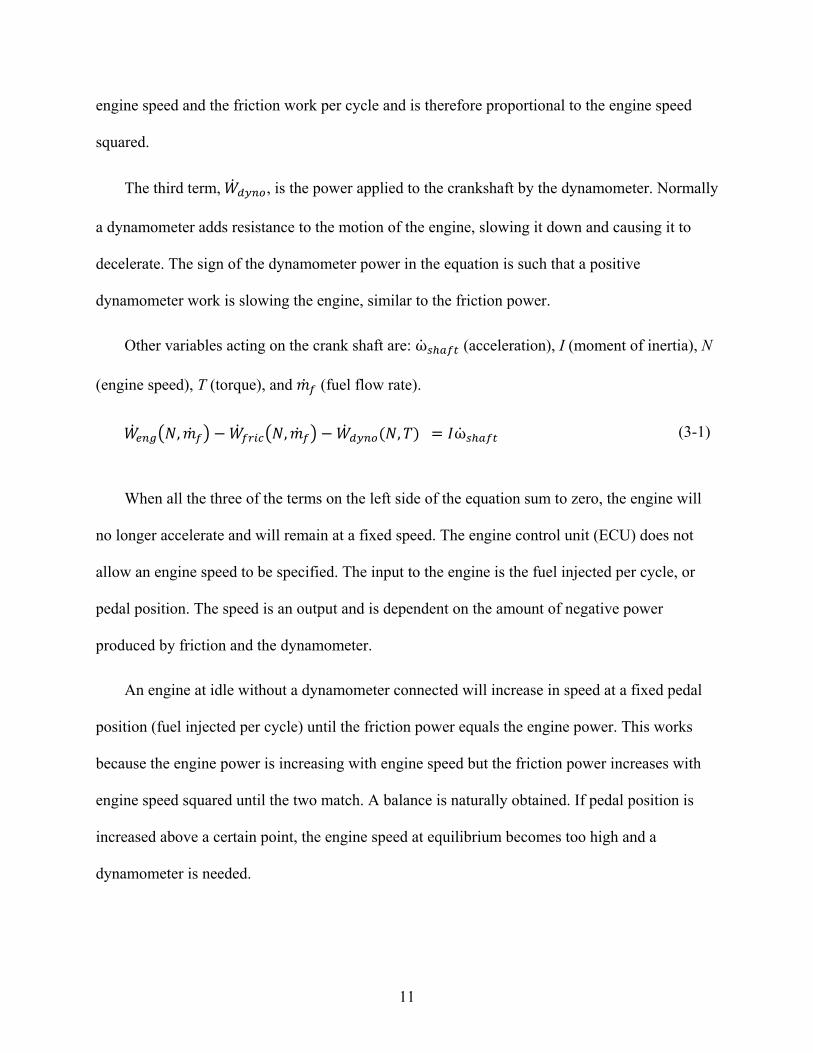
The third term, ��𝑊𝑑𝑑𝑑𝑑𝑒𝑒𝑜𝑜, is the power applied to the crankshaft by the dynamometer. Normally
a dynamometer adds resistance to the motion of the engine, slowing it down and causing it to
decelerate. The sign of the dynamometer power in the equation is such that a positive
dynamometer work is slowing the engine, similar to the friction power.
Other variables acting on the crank shaft are: ω𝑎𝑎ℎ𝑎𝑎𝑓𝑓𝑤𝑤 (acceleration), I (moment of inertia), N
(engine speed), T (torque), and ��𝑚𝑓𝑓 (fuel flow rate).
��𝑊𝑟𝑟𝑒𝑒𝑒𝑒�𝑁𝑁, ��𝑚𝑓𝑓� − ��𝑊𝑓𝑓𝑟𝑟𝑤𝑤𝑓𝑓�𝑁𝑁, ��𝑚𝑓𝑓� − ��𝑊𝑑𝑑𝑑𝑑𝑒𝑒𝑜𝑜(𝑁𝑁,𝑇𝑇) = 𝐼𝐼ω𝑎𝑎ℎ𝑎𝑎𝑓𝑓𝑤𝑤 (3-1)
When all the three of the terms on the left side of the equation sum to zero, the engine will
no longer accelerate and will remain at a fixed speed. The engine control unit (ECU) does not
allow an engine speed to be specified. The input to the engine is the fuel injected per cycle, or
pedal position. The speed is an output and is dependent on the amount of negative power
produced by friction and the dynamometer.
An engine at idle without a dynamometer connected will increase in speed at a fixed pedal
position (fuel injected per cycle) until the friction power equals the engine power. This works
because the engine power is increasing with engine speed but the friction power increases with
engine speed squared until the two match. A balance is naturally obtained. If pedal position is
increased above a certain point, the engine speed at equilibrium becomes too high and a
dynamometer is needed.
12
The custom built AC motoring dynamometer, purchased from Dyne Systems (formerly
known as Taylor Dynamometer), has two modes of operation. A “motoring mode” which allows
the dynamometer power to be added or subtracted to the system (��𝑊𝑑𝑑𝑑𝑑𝑒𝑒𝑜𝑜 can be positive or
negative) and “absorb only” mode where the dynamometer power is always working opposite
the engine. Either of these modes can be selected from the “Dyno Control” menu where the
engine speed is also selected.
When the engine is in absorb only mode, it can be controlled in one of two ways. First, the
user specifies the desired output speed of the system and the pedal position of fuel injected per
cycle. The dynamometer controller then adjusts the amount of torque, or braking force, required
to make the brake power produce a net power of zero. Second, the user specifies the desired
engine output speed and fixes the braking force (torque) desired and the dynamometer controller
adjusts the pedal position until the power is at a net of zero for the specified speed. Note that for
both cases, speed is an input to the dynamometer, not the engine.
To use the first control method, the user selects “throttle position” on the Dyne systems
control menu and specifies a number between 0 and 100%. The term throttle position applies to
spark ignition engines which use a throttle to control the fuel added per cycle. Diesel engines do
not have throttles and so the user should think of this command as pedal position. To use the
second method of control, the user should select “torque control” and specify the output torque
desired.
For purposes of relating a dynamometer to every day experience, consider the dynamometer
as a hill. If you desire to run a car at 2000 RPM, you can adjust the pedal position while driving
down the road until the car is at 2000 RPM. This allows the engine to be studied at a fixed
engine speed. Going up a hill requires an increase in pedal position to reach the same speed. The
13
dynamometer is like a variable hill allowing different pedal positions (fuel flows) to be studied.
The Dyne Systems controls allow the user to specify the steepness of the hill (both uphill or
downhill are possible) and adjusts the pedal position to produce the desired speed for that hill; or
it allows the user to specify the pedal position and adjusts the hill steepness to produce the
desired speed.
14
4 METHODS
This chapter first outlines the methods used to design the engine auxiliary systems with the
$20,000 hardware budget. Second, it outlines the methods used to create the instructional
laboratories for the ICE class. Finally, it outlines the methods used to test the parasitic losses of
the water pump and vacuum pump.
Engine Auxiliary Facilities Design Method
An engine test cell is a laboratory used for testing an engine; it is outfitted with an engine
connected to a dynamometer and all auxiliary systems necessary to run the engine The method
for designing the engine auxiliary systems was to first identify the design requirements and
constraints; second, produce potential system designs; third, analyze and evaluate designs; and
finally, select and test the design. Installation of the engine into the test cell will require the
design of the following auxiliary systems:
• Coupling system – driveline to connect the engine to the dynamometer
• Coolant system – A heat exchanger or radiator
• Intake and exhaust system – An air supply, intercooler, and a means of expelling exhaust
from the room
• Fuel system – A fuel tank and means of supplying and measuring fuel to the engine
• Controls and data acquisition system – At a minimum, a means of controlling pedal or
throttle position. Ideally, a system to measure and control a large number of engine
parameters
15
These room systems were supplied with the test facility. They were not part of the thesis
design, but were considered as design constraints.
• An intake air supply and variable frequency drive (VFD) exhaust fan duct system
• A motoring AC dynamometer
• A slotted floor for engine mounting, control room, and observation window
• A chilled water system with specified flow rates
Design of the auxiliary systems required that the room and engine capabilities be
considered. The room systems included the dynamometer, chilled water cooling system, exhaust
vent, and room air supply. The room specifications are summarized in Table 4-1 along with the
respective power capacities of each system.
Table 4-1: Capacity of Engine Facility Dynamometer, Cooling, and Air Intake/Exhaust Systems System Maximum Capacity Power Capacity
AC Dynamometer 1100 N-m
3200 RPM
342 kW
Chilled Water Cooling Capacity 15 gpm
Tin = 18℃
∆𝑇𝑇 = 40℃
157 kW
Air Intake/Exhaust System (Supply)
With 10:1 air to exhaust ratio
2000 SCFM (supplied)
200 SCFM (for combustion)
58 kW
The following section outlines the design constraints created by the laboratory then the
engine design requirements will be outlined.
16
4.1.1 Design Constraints by the Room
The room contained the AC dynamometer, air intake and exhaust fans, and chilled water
cooling systems. Each of these subsystems was evaluated to understand the engine power that
could be enabled based on the respective system specifications.
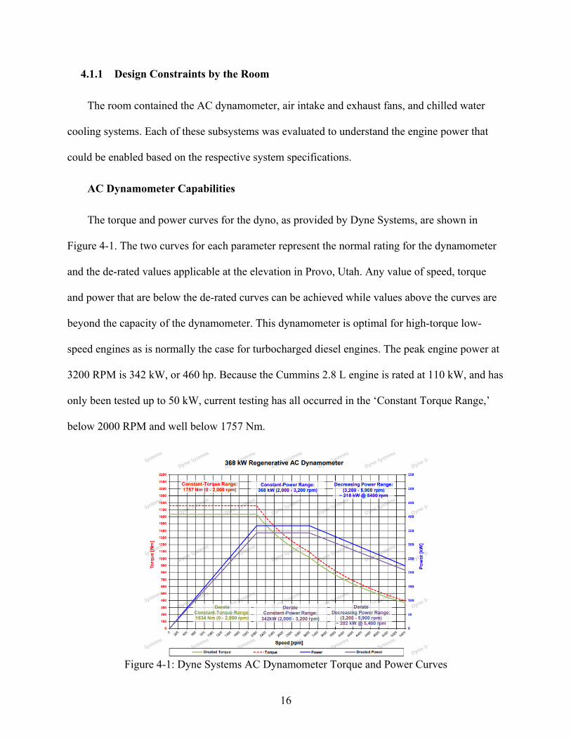
AC Dynamometer Capabilities
The torque and power curves for the dyno, as provided by Dyne Systems, are shown in
Figure 4-1. The two curves for each parameter represent the normal rating for the dynamometer
and the de-rated values applicable at the elevation in Provo, Utah. Any value of speed, torque
and power that are below the de-rated curves can be achieved while values above the curves are
beyond the capacity of the dynamometer. This dynamometer is optimal for high-torque low-
speed engines as is normally the case for turbocharged diesel engines. The peak engine power at
3200 RPM is 342 kW, or 460 hp. Because the Cummins 2.8 L engine is rated at 110 kW, and has
only been tested up to 50 kW, current testing has all occurred in the ‘Constant Torque Range,’
below 2000 RPM and well below 1757 Nm.
Figure 4-1: Dyne Systems AC Dynamometer Torque and Power Curves
17
Chilled Water Cooling System
The test cell room is supplied with chilled cooling water that is returned to a building heat
exchanger and cooled by the universities central heating and cooling plant. The water flow
capacity for the current regulator in the room is 56.85 L/min (15 gpm). Assuming a maximum
allowable temperature rise of 40 oC, the heating capacity for the average temperature of water,
and the mass flow, the maximum cooling capacity of the heat exchanger was calculated to be
157 kW. Detailed engine lab power capacity calculations can be found in Appendix E.
Air and Exhaust Fan Capacity
The air capacity for the room was specified to be 2000 SCFM, which is large enough to
supply a 570 kW diesel engine running at max load. This was the power originally thought
capable for the room.
After running the installed engine, it was discovered that the exhaust duct work required the
air be diluted with additional air in order to keep the exhaust temperature below 70 oC. An
assumption was made that the exhaust would need to be diluted at a ratio of 10:1 parts air to
exhaust. This leaves the air flow available for combustion use in the engine to be 200 SCFM.
Diesel engines are never run at a stoichiometric (14.7:1) air to fuel ratio, so a conservative value
just over two times larger than the stoichiometric mass flow of air to mass flow of fuel ratio of
30:1 was used to calculate the amount of fuel that could be burned with the 200 SCFM supply.
This calculation showed the power capacity of the intake/exhaust system to be 58 kW. If the
room rollup-door is opened, the supply is increased and higher powers are enabled. Detailed
calculations of engine lab power capacity as a result of intake and exhaust system components
can be found in Appendix E.
18
4.1.2 Design Requirements
Two engines were considered as engine donations, a Cummins 2.8 L and a Cummins 5.0 L
engine. The torque, speed, and power at peak torque and maximum power conditions for each
engine are shown in Table 4-2. The power requirements of the 5.0L engine are seen to more
completely utilize the capabilities of the dynamometer. The auxiliary systems were specified to
work for the Cummins 5.0 L engine as the upper design requirement and for the Cummins 2.8 L
engine for the minimum design requirement. Appendix F. demonstrates the data sheets for the
Cummins 2.8 L and 5.0 L engines.
Table 4-2: Ratings of Cummins 2.8 L/5.0 L Engines at Peak Torque and Maximum Power Conditions
Engine Parameter Peak Torque Maximum Power
Cummins 2.8 L Engine Torque
Speed
Power
360 N-m
1500 RPM
56 kW
360 N-m
2900 RPM
110 kW
Cummins 5.0 L Engine Torque
Speed
Power
759 N-m
2000 RPM
159 kW
613 N-m
3200 RPM
205 kW
Design for the engine coupling, cooling, fuel, and intake/exhaust systems were designed to
meet the power requirements of the larger 5.0 L engine to maximize the utilization of the room
capacity. Once the engine was known, many system components required modifications in order
to connect to the 2.8 L engine. The systems are designed to meet the power requirements of both
engines, but interface modifications will be necessary if installing the Cummins 5.0 L, or another
engine in the future. A summary of power requirements is given in Table 4-3.
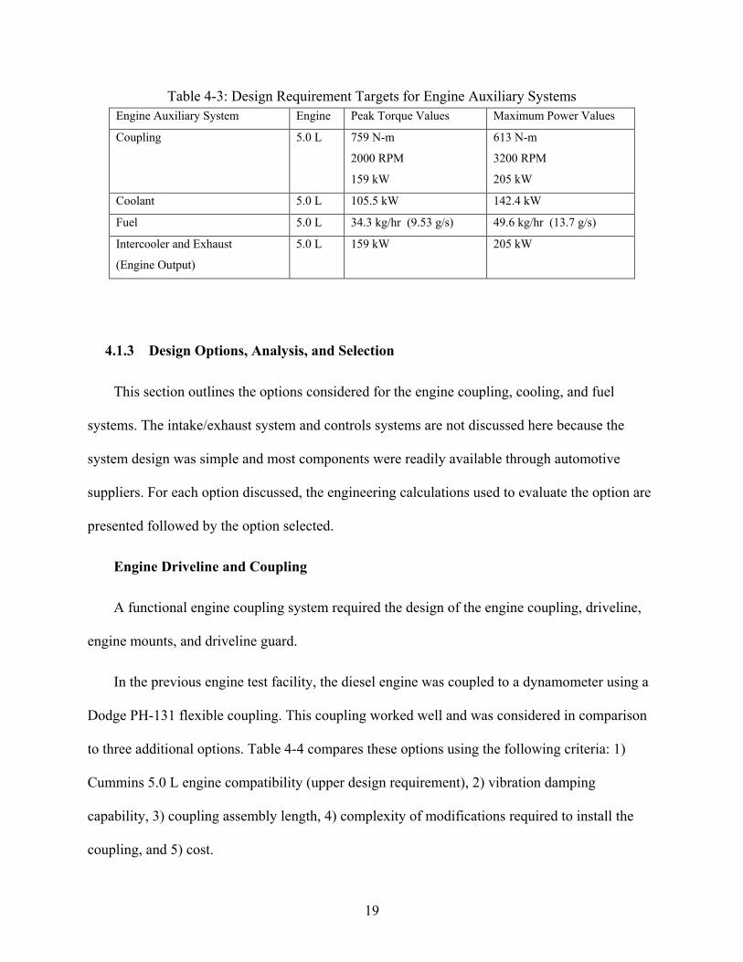
19
Table 4-3: Design Requirement Targets for Engine Auxiliary Systems Engine Auxiliary System Engine Peak Torque Values Maximum Power Values
Coupling 5.0 L 759 N-m
2000 RPM
159 kW
613 N-m
3200 RPM
205 kW
Coolant 5.0 L 105.5 kW 142.4 kW
Fuel 5.0 L 34.3 kg/hr (9.53 g/s) 49.6 kg/hr (13.7 g/s)
Intercooler and Exhaust
(Engine Output)
5.0 L 159 kW 205 kW
4.1.3 Design Options, Analysis, and Selection
This section outlines the options considered for the engine coupling, cooling, and fuel
systems. The intake/exhaust system and controls systems are not discussed here because the
system design was simple and most components were readily available through automotive
suppliers. For each option discussed, the engineering calculations used to evaluate the option are
presented followed by the option selected.
Engine Driveline and Coupling
A functional engine coupling system required the design of the engine coupling, driveline,
engine mounts, and driveline guard.
In the previous engine test facility, the diesel engine was coupled to a dynamometer using a
Dodge PH-131 flexible coupling. This coupling worked well and was considered in comparison
to three additional options. Table 4-4 compares these options using the following criteria: 1)
Cummins 5.0 L engine compatibility (upper design requirement), 2) vibration damping
capability, 3) coupling assembly length, 4) complexity of modifications required to install the
coupling, and 5) cost.
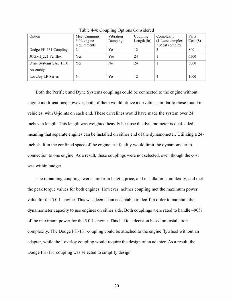
20
Table 4-4: Coupling Options Considered Option Meet Cummins
5.0L engine requirements
Vibration Damping
Coupling Length (in)
Complexity (1 Least complex 5 Most complex)
Parts Cost ($)
Dodge PH-131 Coupling No Yes 12 3 800
JCGMI_221 Periflex Yes Yes 24 1 6500
Dyne Systems SAE 1550
Assembly
Yes No 24 1 5000
LoveJoy LF-Series No Yes 12 4 1000
Both the Periflex and Dyne Systems couplings could be connected to the engine without
engine modifications; however, both of them would utilize a driveline, similar to those found in
vehicles, with U-joints on each end. These drivelines would have made the system over 24
inches in length. This length was weighted heavily because the dynamometer is dual-sided,
meaning that separate engines can be installed on either end of the dynamometer. Utilizing a 24-
inch shaft in the confined space of the engine test facility would limit the dynamometer to
connection to one engine. As a result, these couplings were not selected, even though the cost
was within budget.
The remaining couplings were similar in length, price, and installation complexity, and met
the peak torque values for both engines. However, neither coupling met the maximum power
value for the 5.0 L engine. This was deemed an acceptable tradeoff in order to maintain the
dynamometer capacity to use engines on either side. Both couplings were rated to handle ~90%
of the maximum power for the 5.0 L engine. This led to a decision based on installation
complexity. The Dodge PH-131 coupling could be attached to the engine flywheel without an
adapter, while the LoveJoy coupling would require the design of an adapter. As a result, the
Dodge PH-131 coupling was selected to simplify design.
21
Some design modifications were needed in order to connect the engine to the dynamometer
with the PH-131 coupling. 1) The existing flywheel had to be drilled and tapped with an SAE
11.5 bolt pattern to attach the flexible element. 2) A shaft was designed to transmit power
between the engine and dynamometer. 3) Engine mounts needed to be adjustable to align the
engine and dynamometer shafts, and 4) Finally, a driveline guard needed to be designed and
fabricated for safety.
Driveline Shaft Design
A simple keyed shaft was designed to connect the PH-131 Flexible coupling to the HBM
T40B adapter. Calculations were performed to obtain a minimum diameter for a mild steel shaft
to sustain the maximum torque of 759 N-m. The equation for maximum torque on a solid shaft
was solved for minimum shaft diameter and is shown in Equation (4-1), where D is diameter, T
is torque, and 𝜏𝜏 is shear stress of the shaft material.
𝐷𝐷𝑝𝑝𝑤𝑤𝑒𝑒 = �
16𝜏𝜏𝑝𝑝𝑎𝑎𝑚𝑚
𝜋𝜋𝑇𝑇𝑝𝑝𝑎𝑎𝑚𝑚�1/3
(4-1)
These calculations showed a minimum shaft diameter of 1.20-inches to support 759 N-m. A
larger 2.5-inch shaft was selected to achieve a single diameter shaft that could connect to the
flexible element on one side, and the HBM T40 B adapter on the other.
Engine Mount Design
The flexible rubber coupling was specified to support up to 1° of angular misalignment
between the engine crankshaft and the dynamometer; Equation (4-2) shows the allowable
misalignment as a function of the shaft length. For the selected shaft length of 12.5-inch, the total
allowable misalignment is 0.21-inches.
22
𝑦𝑦 = 𝐿𝐿 ∗ 𝑇𝑇𝑇𝑇𝐸𝐸(1°) (4-2)
In order to keep engine vibrations from causing excess shaft misalignment, the motor
mounts were designed to be solid, rather than absorptive. This will minimize the stress
transmitted to the dynamometer. The engine stands and mounts must allow for adjustment to
ensure that the engine can be aligned with the dynamometer.
Driveline Guard Design
The requirement for the driveline guard was to surround the length of the driveshaft from
the engine to the dynamometer in order to reduce the possibility of items contacting, or being
caught in the driveshaft. The driveshaft guard will also shield bolts or small parts that might
come loose or be dispelled from the driveshaft from a free trajectory across the room. The shield
should remove energy from the driveshaft should it come loose from the coupling, but it is not
intended to completely contain the shaft.
Engine Cooling System Design
Two options were considered for the engine cooling system. A radiator (water to air heat
exchanger) or a water to water heat exchanger. A radiator would reject heat from the coolant into
the test lab further increasing the temperature in the exhaust duct. The water to water heat
exchanger was considered a better option because the building provides chilled water that would
remove the heat from the room.
The engine cooling system design was centered around the purchase of a heat exchanger
capable of removing the maximum heat load from the Cummins 5.0 L engine of 142.4 kW.
Approximate thermodynamic calculations were performed to verify supplier quotes and a
commercial heat exchanger was identified by working with the Thermal Transfer Systems
23
(TTS), a supplier that was used for the previous diesel engine heat exchanger. Quotes for both a
shell and tube heat exchanger and a plate heat exchanger were received. Both heat exchangers
were similar in cost, but the plate heat exchanger was selected because of its lower pressure drop.
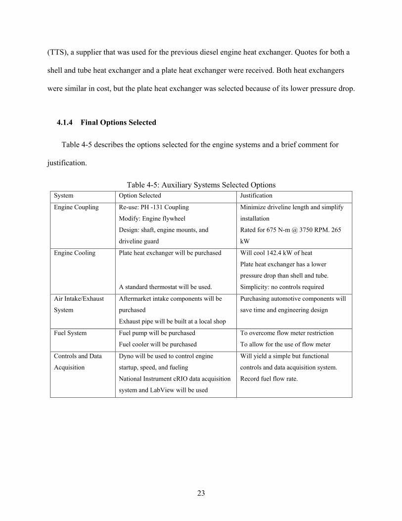
4.1.4 Final Options Selected
Table 4-5 describes the options selected for the engine systems and a brief comment for
justification.
Table 4-5: Auxiliary Systems Selected Options System Option Selected Justification
Engine Coupling Re-use: PH -131 Coupling
Modify: Engine flywheel
Design: shaft, engine mounts, and
driveline guard
Minimize driveline length and simplify
installation
Rated for 675 N-m @ 3750 RPM. 265
kW
Engine Cooling Plate heat exchanger will be purchased
A standard thermostat will be used.
Will cool 142.4 kW of heat
Plate heat exchanger has a lower
pressure drop than shell and tube.
Simplicity: no controls required
Air Intake/Exhaust
System
Aftermarket intake components will be
purchased
Exhaust pipe will be built at a local shop
Purchasing automotive components will
save time and engineering design
Fuel System Fuel pump will be purchased
Fuel cooler will be purchased
To overcome flow meter restriction
To allow for the use of flow meter
Controls and Data
Acquisition
Dyno will be used to control engine
startup, speed, and fueling
National Instrument cRIO data acquisition
system and LabView will be used
Will yield a simple but functional
controls and data acquisition system.
Record fuel flow rate.
24
Lab Testing Methods
The objectives of the instructional laboratories for the ICE class are to measure engine brake
torque, power, fuel flow, and emissions as a function of fuel flow rate, or pedal position, at a
constant engine speed. This was accomplished by running the engine at 1500 RPM, taking fuel
flow, torque, and speed data at increasing fuel loads and calculating brake fuel conversion
efficiency. See Appendix G. for the diesel engine operating instructions.
Measuring Parasitic Losses of the Water Pump
A method was developed to test the power input and output of the Cummins 2.8 L water
pump corresponding to an engine speed range of 300 - 3000 RPM. A torque transducer and
speed encoder were used to quantify power input; a flow meter and three individual pressure
transducers were used to quantify the water pump power output. The ratio of power output to
power input was used to calculate a pump efficiency. Both open and closed thermostat cases
were simulated.
Figure 4-2 is a schematic diagram of the water pump test setup. The left side of the figure
shows the water flow route used to simulate open and closed thermostat cases while the right
side shows how data were recorded. The heat exchanger normally used to cool the coolant
exiting the engine was replaced with a radiator to simulate the pressure drop of a functioning
engine. The open thermostat test case was simulated by removing the thermostat and plugging
the bypass tube, which forced the entire water flow to return through the radiator. There was no
pressure drop across the thermostat, because it was removed, so reported values represent the
minimum pumping work required to push a fluid across the radiator. The closed thermostat test
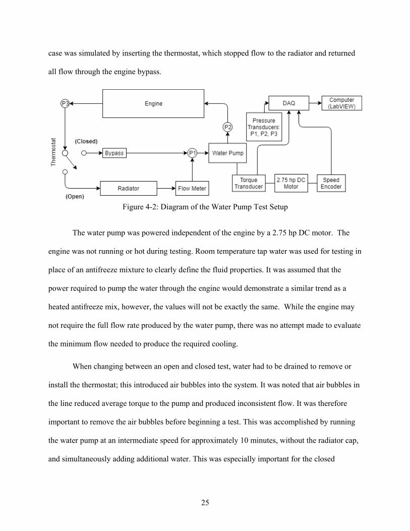
25
case was simulated by inserting the thermostat, which stopped flow to the radiator and returned
all flow through the engine bypass.
Figure 4-2: Diagram of the Water Pump Test Setup
The water pump was powered independent of the engine by a 2.75 hp DC motor. The
engine was not running or hot during testing. Room temperature tap water was used for testing in
place of an antifreeze mixture to clearly define the fluid properties. It was assumed that the
power required to pump the water through the engine would demonstrate a similar trend as a
heated antifreeze mix, however, the values will not be exactly the same. While the engine may
not require the full flow rate produced by the water pump, there was no attempt made to evaluate
the minimum flow needed to produce the required cooling.
When changing between an open and closed test, water had to be drained to remove or
install the thermostat; this introduced air bubbles into the system. It was noted that air bubbles in
the line reduced average torque to the pump and produced inconsistent flow. It was therefore
important to remove the air bubbles before beginning a test. This was accomplished by running
the water pump at an intermediate speed for approximately 10 minutes, without the radiator cap,
and simultaneously adding additional water. This was especially important for the closed
26
thermostat scenarios. The radiator cap was opened between tests to ensure a consistent starting
pressure.
As seen in the right side of Figure 4-2, pressure, torque, and speed data were sent to a
DAQ system and recorded. See Table 4-6 for DAQ and sensor details. Data were taken at a
frequency of 100 Hz and averaged for 2 seconds (200 sampled points); the average and standard
deviation were displayed on a monitor. When standard deviation of the water pump speed for the
200 sampled points was less than 2 RPM, the system was assumed to be at steady state and the
average pressures were recorded. A sweep of pump speeds was performed with one averaged
point recorded at each speed. Multiple sweeps were then collected for the open and closed
conditions on multiple days for a range of speeds that varied from below the engine idle speed to
the speed at maximum power.
A table of sensors and transducers used for the measurements along with the measurement
range and resolution is given in Table 4-6. The measurement equipment was borrowed from the
Department of Mechanical Engineering.
Table 4-6: Specifications for Sensors Used to Test Parasitic Losses Component Range Resolution
Schlenker Ent. Torque Transducer 0-20 N-m ±0.2% FS (0.04 N-m)
Quadrature Speed Encoder TRD-SH1000BD 0-6000 RPM 1000 PPR, 200 kHz response
National Instruments DAQ cRIO-9074 8-Slot 100 MHz CPU, 128 MB DRAM
Absolute Pressure Transducer (S/N 12506) 0-50 psi ±0.2% FS (0.1 psi) @ 500 Hz
Copal Electronics PA-500-502G Pressure
Transducers (2)
0-490 kPa ±0.5% FS (2.5 kPa) @ 1000 Hz
Digiten Water Flow Sensor Model: FL-1608 10-200 L/min ±0.2% FS (4 L/min) @ 40 Hz
27
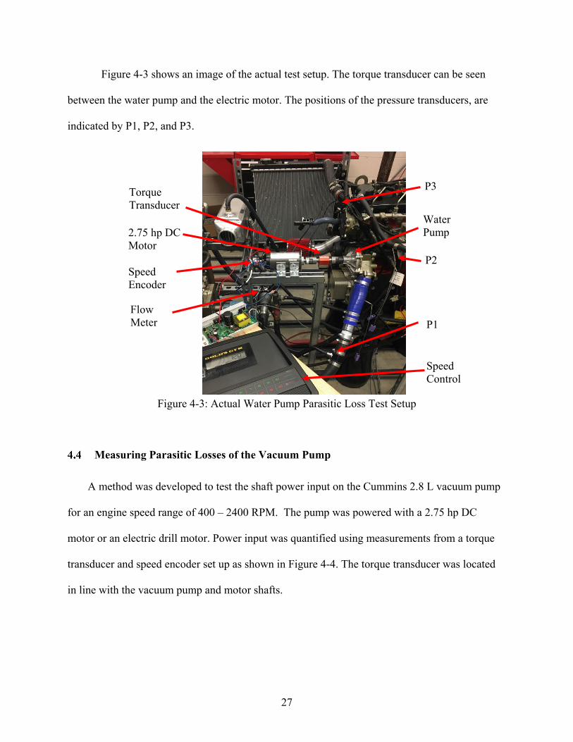
Figure 4-3 shows an image of the actual test setup. The torque transducer can be seen
between the water pump and the electric motor. The positions of the pressure transducers, are
indicated by P1, P2, and P3.
Figure 4-3: Actual Water Pump Parasitic Loss Test Setup
Measuring Parasitic Losses of the Vacuum Pump
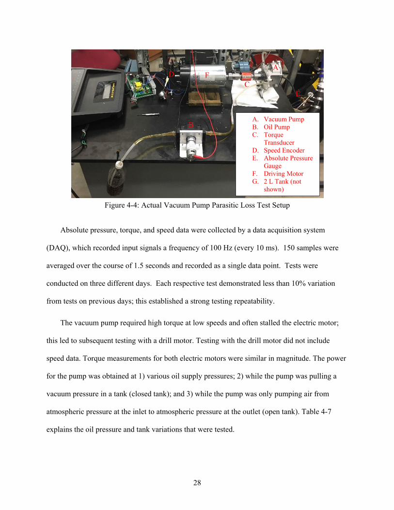
A method was developed to test the shaft power input on the Cummins 2.8 L vacuum pump
for an engine speed range of 400 – 2400 RPM. The pump was powered with a 2.75 hp DC
motor or an electric drill motor. Power input was quantified using measurements from a torque
transducer and speed encoder set up as shown in Figure 4-4. The torque transducer was located
in line with the vacuum pump and motor shafts.
P1
P2
P3
Speed Control
Torque Transducer
Speed Encoder
Flow Meter
2.75 hp DC Motor
Water Pump
28
Figure 4-4: Actual Vacuum Pump Parasitic Loss Test Setup
Absolute pressure, torque, and speed data were collected by a data acquisition system
(DAQ), which recorded input signals a frequency of 100 Hz (every 10 ms). 150 samples were
averaged over the course of 1.5 seconds and recorded as a single data point. Tests were
conducted on three different days. Each respective test demonstrated less than 10% variation
from tests on previous days; this established a strong testing repeatability.
The vacuum pump required high torque at low speeds and often stalled the electric motor;
this led to subsequent testing with a drill motor. Testing with the drill motor did not include
speed data. Torque measurements for both electric motors were similar in magnitude. The power
for the pump was obtained at 1) various oil supply pressures; 2) while the pump was pulling a
vacuum pressure in a tank (closed tank); and 3) while the pump was only pumping air from
atmospheric pressure at the inlet to atmospheric pressure at the outlet (open tank). Table 4-7
explains the oil pressure and tank variations that were tested.
A
B
C D
E
F
A. Vacuum Pump B. Oil Pump C. Torque
Transducer D. Speed Encoder E. Absolute Pressure
Gauge F. Driving Motor G. 2 L Tank (not
shown)
29
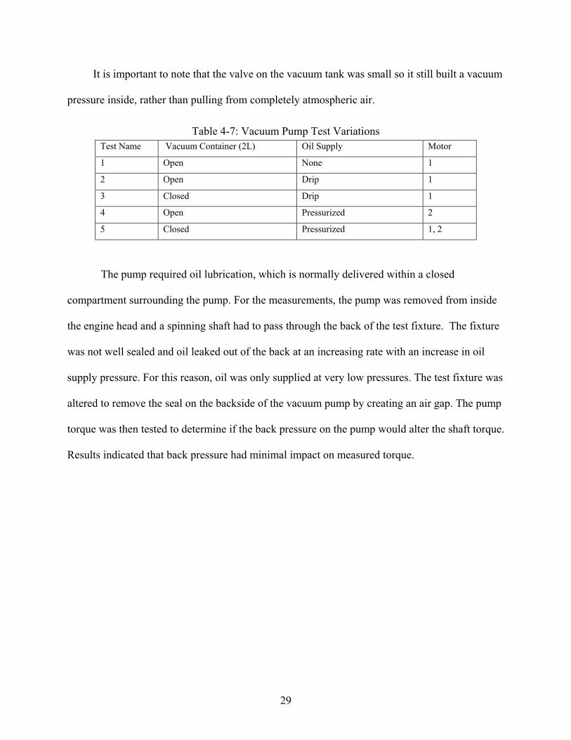
It is important to note that the valve on the vacuum tank was small so it still built a vacuum
pressure inside, rather than pulling from completely atmospheric air.
Table 4-7: Vacuum Pump Test Variations Test Name Vacuum Container (2L) Oil Supply Motor
1 Open None 1
2 Open Drip 1
3 Closed Drip 1
4 Open Pressurized 2
5 Closed Pressurized 1, 2
The pump required oil lubrication, which is normally delivered within a closed
compartment surrounding the pump. For the measurements, the pump was removed from inside
the engine head and a spinning shaft had to pass through the back of the test fixture. The fixture
was not well sealed and oil leaked out of the back at an increasing rate with an increase in oil
supply pressure. For this reason, oil was only supplied at very low pressures. The test fixture was
altered to remove the seal on the backside of the vacuum pump by creating an air gap. The pump
torque was then tested to determine if the back pressure on the pump would alter the shaft torque.
Results indicated that back pressure had minimal impact on measured torque.
30
5 RESULTS AND DISCUSSION
This chapter presents results for the major objectives of this work. First, the resulting engine
test cell auxiliary system setup is presented; total hardware costs for these systems totaled $8,100
of the $20,000 budget. A system schematic of the implemented systems, provides a description
of each system, shows rated performance of individual systems components, and ends with
measured performance results demonstrating a working setup. Second, the capacity of the system
to take fuel flow, torque, power, and speed data for the engine labs is demonstrated with sample
plots. Finally, the results for parasitic losses for the water and vacuum pumps are presented and
compared to vehicle drive cycles to explore the overall efficiency improvements possible by
removing the pumps.
Engine Lab Setup
A schematic diagram of the test cell setup is shown in Figure 5-1. The setup is divided into
five systems: 1) a driveline coupling system (which includes the guard and motor mounts), 2) an
engine cooling system, 3) an air intake and exhaust system, 4) a fuel system, and 5) a controls
and data acquisition system. The schematic of the setup is a view of the engine from above, with
the top of the figure being the east side of the room; the building coolant system is closest to the
control room. The fuel system is located on the bottom of the figure, or the west side of the
room. The diagram shows the general location of auxiliary system components and the direction
of flow for coolant, air, exhaust, and fuel.
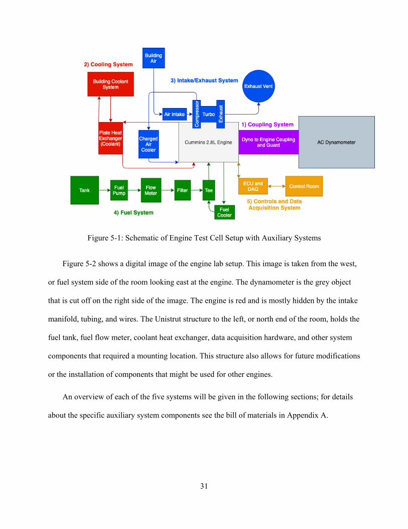
31
Figure 5-1: Schematic of Engine Test Cell Setup with Auxiliary Systems
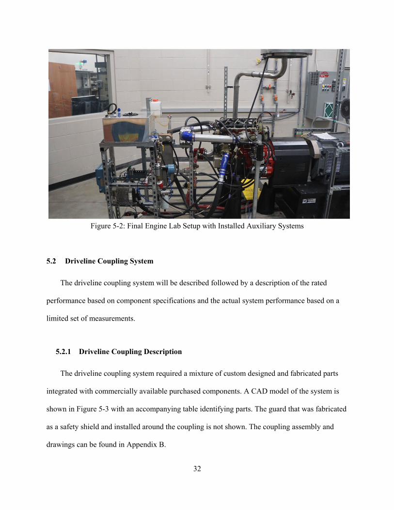
Figure 5-2 shows a digital image of the engine lab setup. This image is taken from the west,
or fuel system side of the room looking east at the engine. The dynamometer is the grey object
that is cut off on the right side of the image. The engine is red and is mostly hidden by the intake
manifold, tubing, and wires. The Unistrut structure to the left, or north end of the room, holds the
fuel tank, fuel flow meter, coolant heat exchanger, data acquisition hardware, and other system
components that required a mounting location. This structure also allows for future modifications
or the installation of components that might be used for other engines.
An overview of each of the five systems will be given in the following sections; for details
about the specific auxiliary system components see the bill of materials in Appendix A.
32
Figure 5-2: Final Engine Lab Setup with Installed Auxiliary Systems
Driveline Coupling System
The driveline coupling system will be described followed by a description of the rated
performance based on component specifications and the actual system performance based on a
limited set of measurements.
5.2.1 Driveline Coupling Description
The driveline coupling system required a mixture of custom designed and fabricated parts
integrated with commercially available purchased components. A CAD model of the system is
shown in Figure 5-3 with an accompanying table identifying parts. The guard that was fabricated
as a safety shield and installed around the coupling is not shown. The coupling assembly and
drawings can be found in Appendix B.
33
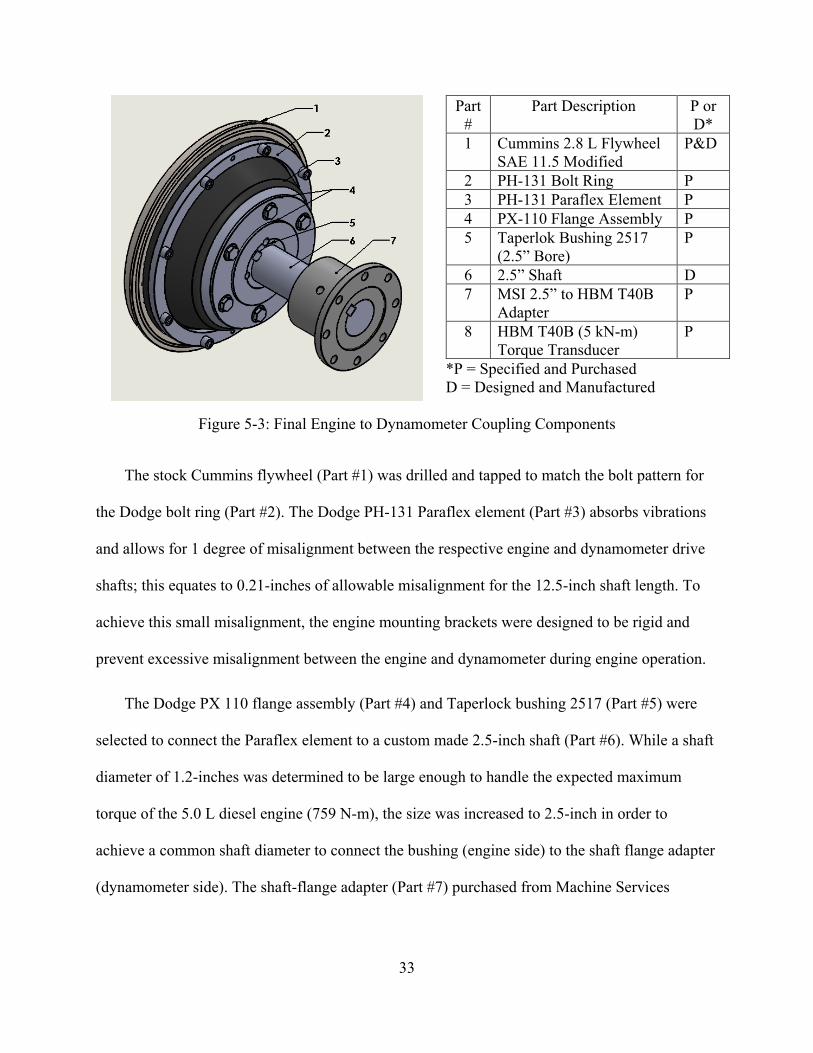
Part #
Part Description P or D*
1 Cummins 2.8 L Flywheel SAE 11.5 Modified
P&D
2 PH-131 Bolt Ring P 3 PH-131 Paraflex Element P 4 PX-110 Flange Assembly P 5 Taperlok Bushing 2517
(2.5” Bore) P
6 2.5” Shaft D 7 MSI 2.5” to HBM T40B
Adapter P
8 HBM T40B (5 kN-m) Torque Transducer
P
*P = Specified and Purchased D = Designed and Manufactured
Figure 5-3: Final Engine to Dynamometer Coupling Components
The stock Cummins flywheel (Part #1) was drilled and tapped to match the bolt pattern for
the Dodge bolt ring (Part #2). The Dodge PH-131 Paraflex element (Part #3) absorbs vibrations
and allows for 1 degree of misalignment between the respective engine and dynamometer drive
shafts; this equates to 0.21-inches of allowable misalignment for the 12.5-inch shaft length. To
achieve this small misalignment, the engine mounting brackets were designed to be rigid and
prevent excessive misalignment between the engine and dynamometer during engine operation.
The Dodge PX 110 flange assembly (Part #4) and Taperlock bushing 2517 (Part #5) were
selected to connect the Paraflex element to a custom made 2.5-inch shaft (Part #6). While a shaft
diameter of 1.2-inches was determined to be large enough to handle the expected maximum
torque of the 5.0 L diesel engine (759 N-m), the size was increased to 2.5-inch in order to
achieve a common shaft diameter to connect the bushing (engine side) to the shaft flange adapter
(dynamometer side). The shaft-flange adapter (Part #7) purchased from Machine Services
34
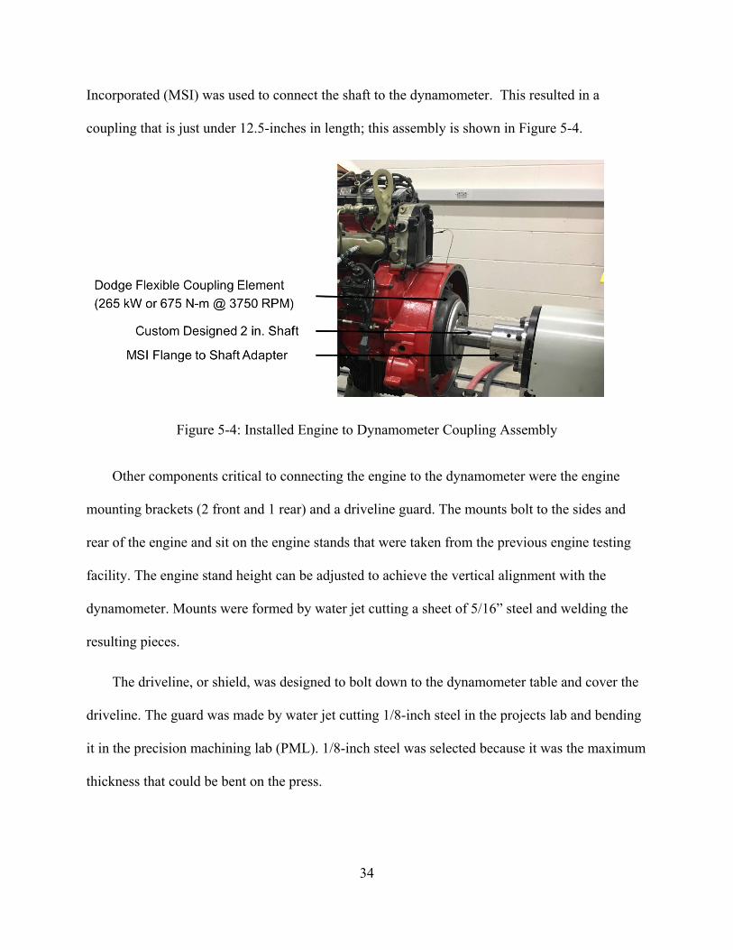
Incorporated (MSI) was used to connect the shaft to the dynamometer. This resulted in a
coupling that is just under 12.5-inches in length; this assembly is shown in Figure 5-4.
Figure 5-4: Installed Engine to Dynamometer Coupling Assembly
Other components critical to connecting the engine to the dynamometer were the engine
mounting brackets (2 front and 1 rear) and a driveline guard. The mounts bolt to the sides and
rear of the engine and sit on the engine stands that were taken from the previous engine testing
facility. The engine stand height can be adjusted to achieve the vertical alignment with the
dynamometer. Mounts were formed by water jet cutting a sheet of 5/16” steel and welding the
resulting pieces.
The driveline, or shield, was designed to bolt down to the dynamometer table and cover the
driveline. The guard was made by water jet cutting 1/8-inch steel in the projects lab and bending
it in the precision machining lab (PML). 1/8-inch steel was selected because it was the maximum
thickness that could be bent on the press.
35
5.2.2 Driveline Coupling Rated Performance
The engine coupling assembly is limited by thePH-131 flexible element, which is rated for
265 kW, or 675 N-m at 3750 RPM. This flexible element is anticipated to be the first component
to fail in the case of a coupling failure, based on component ratings; element pieces should be
contained within the shield and people are not allowed in the room during operation so safety
should be maintained. It is recommended that the element cracks be checked routinely and the
coupling be replaced if necessary.
5.2.3 Driveline Coupling Measured Performance
The installed driveline coupling has been used to run the engine up to 325 N-m @ 1500
RPM (50 kW). The flexible element showed a series of cracks even though the torque and speed
were below the rated capacity. These cracks are attributed to excessive torque on the coupling
bolts during installation. These bolts were backed off to the correct torque and further testing
showed no lengthening of the cracks. However, due to the need to run the engine labs for the
internal combustion engine class without risk of failure it was decided to not test the maximum
torque and speed of the engine coupling. These cracks should be monitored regularly to know if
the coupling should be replaced.
Coolant System
5.3.1 Coolant System Description
Building coolant passes through a plate heat exchanger and cools the engine water when the
engine thermostat is open. The building coolant and engine coolant enter adjoining, but separate,
channels of the heat exchanger and cools the engine coolant; the two fluids are not mixed. This
36
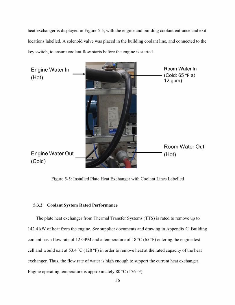
heat exchanger is displayed in Figure 5-5, with the engine and building coolant entrance and exit
locations labelled. A solenoid valve was placed in the building coolant line, and connected to the
key switch, to ensure coolant flow starts before the engine is started.
Figure 5-5: Installed Plate Heat Exchanger with Coolant Lines Labelled
5.3.2 Coolant System Rated Performance
The plate heat exchanger from Thermal Transfer Systems (TTS) is rated to remove up to
142.4 kW of heat from the engine. See supplier documents and drawing in Appendix C. Building
coolant has a flow rate of 12 GPM and a temperature of 18 oC (65 ℉) entering the engine test
cell and would exit at 53.4 oC (128 oF) in order to remove heat at the rated capacity of the heat
exchanger. Thus, the flow rate of water is high enough to support the current heat exchanger.
Engine operating temperature is approximately 80 oC (176 oF).
37
5.3.3 Coolant System Measured Performance
At peak torque (360 N-m @ 1500 RPM [56 kW]), the cooling requirement of the engine is
rated at 32.9 kW, or 58% of the engine power output. The engine was tested up to 325 N-m @
1500 RPM [51 kW], or 91% of total power at peak torque. Because it was operated so close to
the power at peak torque, a conservative assumption was made that the heat rejected by the heat
exchanger was 91% of the 32.9 kW, or 30 kW. The systems cooling capacity could be observed
by monitoring the engine coolant temperature on the Cummins Calterm software; the coolant
temperature fluctuated between 77-86 ℃ as the thermostat opened and closed. It appears that the
thermostat opens completely and closes completely because the temperature can be seen to
increase slowly then decrease rapidly in a matter of approximately 10-15 seconds as the
thermostat opens and the water is cooled in the heat exchanger.
Intake/Exhaust System
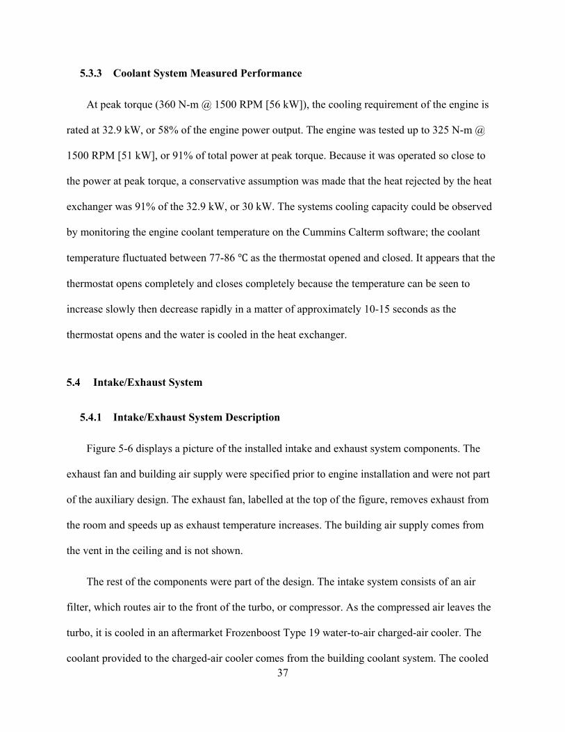
5.4.1 Intake/Exhaust System Description
Figure 5-6 displays a picture of the installed intake and exhaust system components. The
exhaust fan and building air supply were specified prior to engine installation and were not part
of the auxiliary design. The exhaust fan, labelled at the top of the figure, removes exhaust from
the room and speeds up as exhaust temperature increases. The building air supply comes from
the vent in the ceiling and is not shown.
The rest of the components were part of the design. The intake system consists of an air
filter, which routes air to the front of the turbo, or compressor. As the compressed air leaves the
turbo, it is cooled in an aftermarket Frozenboost Type 19 water-to-air charged-air cooler. The
coolant provided to the charged-air cooler comes from the building coolant system. The cooled
38
and charged air then enters the engine at a higher density. The actual temperature of the air
before and after the cooler was not measured, but was checked by touching the hot side and the
cool side after running the engine; the charged air-line upstream of the cooler could only be
touched briefly because of the high temperature while the charged air-line downstream of the
cooler was cool to the touch.
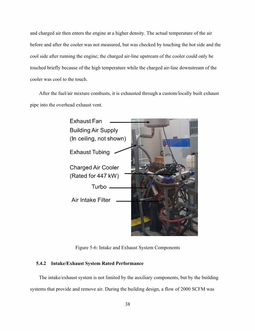
After the fuel/air mixture combusts, it is exhausted through a custom/locally built exhaust
pipe into the overhead exhaust vent.
Figure 5-6: Intake and Exhaust System Components
5.4.2 Intake/Exhaust System Rated Performance
The intake/exhaust system is not limited by the auxiliary components, but by the building
systems that provide and remove air. During the building design, a flow of 2000 SCFM was
39
specified for the test cell. Assuming that the lab is built to specifications and that 10 parts of air
are used to cool one part of exhaust in the exhaust vent, the maximum theoretical power of the
engine with this flow, and the rollup door closed, would be 58.3 kW. The building air supply and
amount needed for dilution is the limiting factor for engine operation currently.
5.4.3 Intake/Exhaust System Measured Performance
It was observed that during engine operation that loads above 2.6 g/s of fuel flow could not
be maintained without opening the roll-up door and allowing outside air to enter the test cell.
This corresponds to a tested engine power limitation of 40 kW. With the roll-up door open, a
higher performance of the test cell design could be evaluated and the Cummins 2.8 L engine was
tested up to a value of 50 kW. (The engine was not tested above 50 kW during development of
the laboratory experiments) These test results demonstrate that the exhaust fan is removing more
air (��𝑚𝐸𝐸𝑚𝑚 𝐻𝐻𝑟𝑟𝑒𝑒𝑤𝑤) than is supplied to the room (��𝑚𝐵𝐵𝑜𝑜𝑤𝑤𝑟𝑟𝑑𝑑𝑤𝑤𝑒𝑒𝑒𝑒 𝑆𝑆𝑜𝑜𝑝𝑝𝑝𝑝𝑟𝑟𝑑𝑑) as shown in Equation (5-1).
��𝑚𝐸𝐸𝑚𝑚 𝐻𝐻𝑟𝑟𝑒𝑒𝑤𝑤 > ��𝑚𝐵𝐵𝑜𝑜𝑤𝑤𝑟𝑟𝑑𝑑𝑤𝑤𝑒𝑒𝑒𝑒 𝑆𝑆𝑜𝑜𝑝𝑝𝑝𝑝𝑟𝑟𝑑𝑑
(5-1)
A portion of the mass air flow delivered to the room enters the engine through the intake,
while the remaining portion exits the room through the exhaust vent and helps dilute, or cool, the
exhaust in the duct; this relationship can be seen in Equation (5-2). The current workaround to
this problem is to increase ��𝑚𝐼𝐼𝑒𝑒𝑤𝑤𝑎𝑎𝐼𝐼𝑟𝑟 by opening the roll-up door. In the future, ��𝑚𝐷𝐷𝑤𝑤𝑟𝑟𝑜𝑜𝑤𝑤𝑤𝑤𝑜𝑜𝑒𝑒 could be
decreased by reducing the exhaust speed, or cooling the exhaust with an additional heat
exchanger.
��𝑚𝐸𝐸𝑚𝑚 𝐻𝐻𝑟𝑟𝑒𝑒𝑤𝑤 > ��𝑚𝐼𝐼𝑒𝑒𝑤𝑤𝑎𝑎𝐼𝐼𝑟𝑟 + ��𝑚𝐷𝐷𝑤𝑤𝑟𝑟𝑜𝑜𝑤𝑤𝑤𝑤𝑜𝑜𝑒𝑒 (5-2)
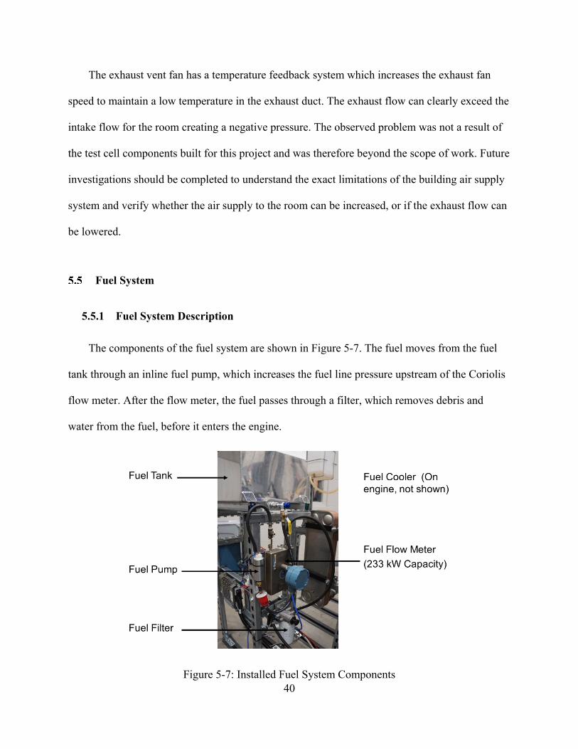
40
The exhaust vent fan has a temperature feedback system which increases the exhaust fan
speed to maintain a low temperature in the exhaust duct. The exhaust flow can clearly exceed the
intake flow for the room creating a negative pressure. The observed problem was not a result of
the test cell components built for this project and was therefore beyond the scope of work. Future
investigations should be completed to understand the exact limitations of the building air supply
system and verify whether the air supply to the room can be increased, or if the exhaust flow can
be lowered.
Fuel System
5.5.1 Fuel System Description
The components of the fuel system are shown in Figure 5-7. The fuel moves from the fuel
tank through an inline fuel pump, which increases the fuel line pressure upstream of the Coriolis
flow meter. After the flow meter, the fuel passes through a filter, which removes debris and
water from the fuel, before it enters the engine.
Figure 5-7: Installed Fuel System Components
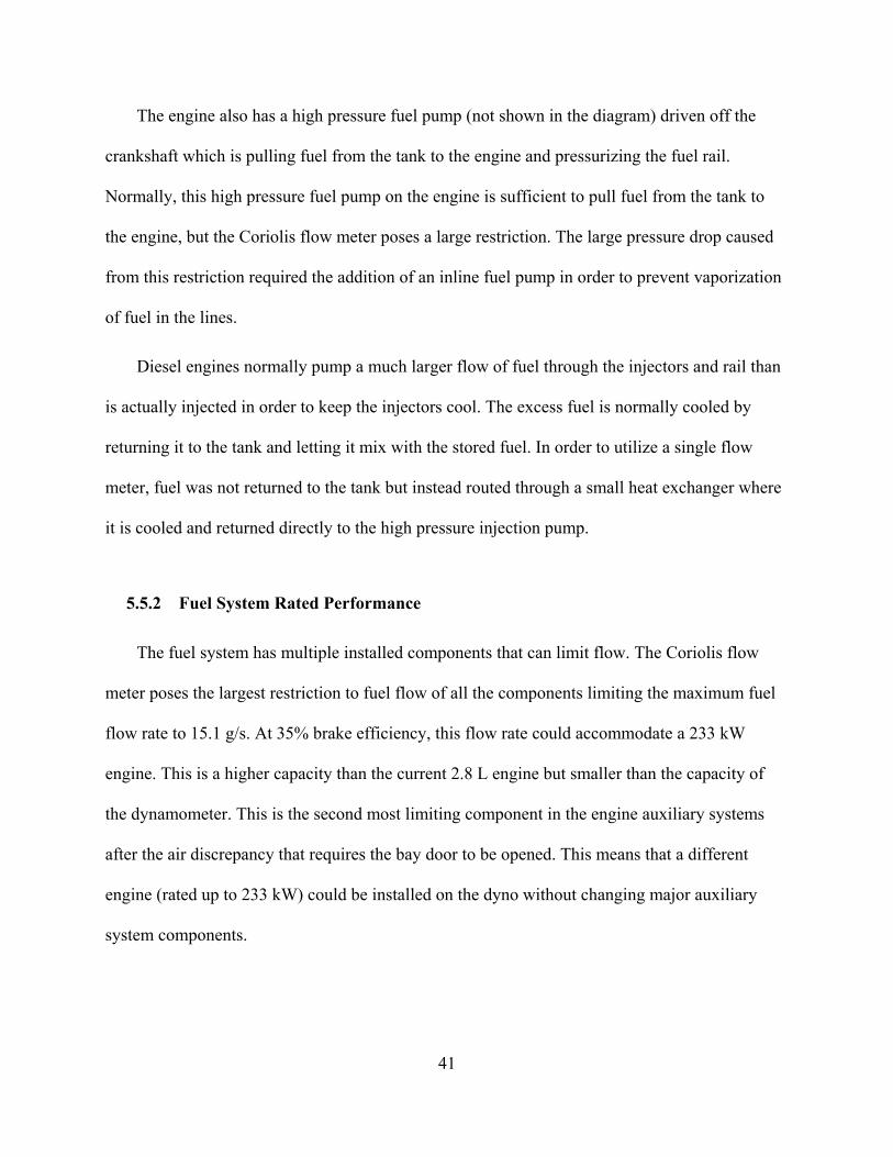
41
The engine also has a high pressure fuel pump (not shown in the diagram) driven off the
crankshaft which is pulling fuel from the tank to the engine and pressurizing the fuel rail.
Normally, this high pressure fuel pump on the engine is sufficient to pull fuel from the tank to
the engine, but the Coriolis flow meter poses a large restriction. The large pressure drop caused
from this restriction required the addition of an inline fuel pump in order to prevent vaporization
of fuel in the lines.
Diesel engines normally pump a much larger flow of fuel through the injectors and rail than
is actually injected in order to keep the injectors cool. The excess fuel is normally cooled by
returning it to the tank and letting it mix with the stored fuel. In order to utilize a single flow
meter, fuel was not returned to the tank but instead routed through a small heat exchanger where
it is cooled and returned directly to the high pressure injection pump.
5.5.2 Fuel System Rated Performance
The fuel system has multiple installed components that can limit flow. The Coriolis flow
meter poses the largest restriction to fuel flow of all the components limiting the maximum fuel
flow rate to 15.1 g/s. At 35% brake efficiency, this flow rate could accommodate a 233 kW
engine. This is a higher capacity than the current 2.8 L engine but smaller than the capacity of
the dynamometer. This is the second most limiting component in the engine auxiliary systems
after the air discrepancy that requires the bay door to be opened. This means that a different
engine (rated up to 233 kW) could be installed on the dyno without changing major auxiliary
system components.
42
5.5.3 Fuel System Measured Performance
Initially, the fuel system was installed without the inline fuel pump. This allowed the engine
to run, but the response time for the Coriolis flow meter was approximately three minutes. With
the pump installed, response times decreased to approximately 30 seconds. It is clear that the fuel
pump has an effect on the dynamic response of the fuel system. It is not clear what portion of the
slow response can be attributed to the flow meter and what is now attributed to the fuel system
dynamics. The maximum fuel flow tested on the engine was 3.06 g/s; higher flows can be tested
in the future.
Controls/DAQ System
5.6.1 Controls/DAQ System Description
Figure 5-8 shows various components contributing to the controls and data acquisition
system. The picture on the left displays the components in the test cell. First, there is the
Cummins engine control unit (ECU), which is the primary control for the engine. Second, Fuel
flow data is currently collected from the Coriolis flow meter via a National Instruments cRIO
9074 data acquisition module and read with a LabVIEW program on the computer in the control
room.
The Control room is shown on the right in the figure and contains the computer and
dynamometer control box. The dynamometer has a control box that is connected to the ECU; this
control box receives torque and speed feedback data from the torque transducer on the
dynamometer and varies the commands to the ECU based on the torque or pedal position
specified by the user. This allows for simple control of the engine with the dynamometer control
box (located in the control room). Brake torque and engine speed are displayed on the control
43
box. Emissions data was taken using a stand-alone gas analyzer. See Appendix D. for the wiring
diagram to connect sensors, data acquisition system, and controls.
Figure 5-8: Left: Engine bay - Engine control unit and data acquisition system. Right: Control room - dynamometer control box, computer with LabVIEW data recording software.
5.6.2 Controls/DAQ System Rated Performance
The HBM T40B torque transducer mounted on the dynamometer is rated to measure torque
up to 5000 N-m, which is much larger than the max rating of 1750 N-m of the dynamometer.
The torque transducer was selected by the dynamometer supplier without appropriate oversight
by BYU before delivery. It was not changed after dynamometer delivery due to cost
considerations.
5.6.3 Controls/DAQ System Measured Performance
Torque and engine speed were successfully measured, displayed, and recorded by hand from
the dynamometer control box. A torque uncertainty of ±3.5 N-m was measured by checking the
44
standard deviation of torque measurements during testing; this uncertainty is due to the torque
transducer’s large measuring range.
Fuel flow rate was collected through the LabVIEW program; in the future, additional sensor
data can be collected through the National Instruments cRIO 9074 expansion slots. Currently
engine torque and speed are shown on the dyno control box and fuel data are read into
LabVIEW.
The Cummins Calterm software limited license allows for the reading of engine data such as
engine temperature and diagnostic codes. Some variables, such as fueling, can be temporarily
altered in the Calterm software, but any long-term calibration changes must be conducted by
Cummins. Using the Calterm software for more than simple monitoring of engine sensors
requires a learning curve as it is Cummins specific and not designed for third parties. For this
reason, Calterm is currently used only to monitor the engine coolant temperature while engine
control is conducted with the dynamometer control box.
Summary of Engine Auxiliary Setup Ratings and Measured Performance
This section summarizes the rated and measured performance of the auxiliary systems (See
Table 5-1) to enable readers to understand necessary changes that would be required to install a
different engine in the test cell. All of the current components are shown to function above the
operating range of the current 2.8 L engine except for the flexible element in the coupling
assembly, which is rated for the engine but was potentially damaged during installation. The
current system has been demonstrated to work for the ICE class laboratory experiments and
capstone design projects. Some power ratings are taken from applicable supplier documents, and
others are calculated in Appendix E.
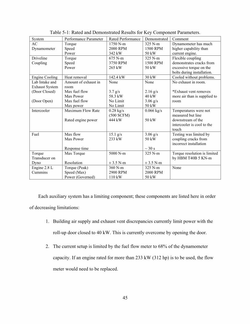
45
Table 5-1: Rated and Demonstrated Results for Key Component Parameters. System Performance Parameter Rated Performance Demonstrated Comment AC Dynamometer
Torque Speed Power
1750 N-m 2000 RPM 342 kW
325 N-m 1500 RPM 50 kW
Dynamometer has much higher capability than current engine.
Driveline Coupling
Torque Speed Power
675 N-m 3750 RPM 265 kW
325 N-m 1500 RPM 50 kW
Flexible coupling demonstrates cracks from excessive torque on the bolts during installation.
Engine Cooling Heat removal 142.4 kW 30 kW Cooled without problems. Lab Intake and Exhaust System (Door Closed) (Door Open)
Amount of exhaust in room Max fuel flow Max Power Max fuel flow Max power
None 3.7 g/s 58.3 kW No Limit No Limit
None 2.16 g/s 40 kW 3.06 g/s 50 kW
No exhaust in room. *Exhaust vent removes more air than is supplied to room
Intercooler Maximum Flow Rate Rated engine power
0.28 kg/s (500 SCFM) 444 kW
0.066 kg/s 50 kW
Temperatures were not measured but line downstream of the intercooler is cool to the touch
Fuel Max flow Max Power Response time
15.1 g/s 233 kW
3.06 g/s 50 kW ~ 30 s
Testing was limited by coupling cracks from incorrect installation
Torque Transducer on Dyno
Max Torque Resolution
5000 N-m ± 3.5 N-m
325 N-m ± 3.5 N-m
Torque resolution is limited by HBM T40B 5 KN-m
Engine 2.8 L Cummins
Torque (Peak) Speed (Max) Power (Governed)
360 N-m 2900 RPM 110 kW
325 N-m 2000 RPM 50 kW
None
Each auxiliary system has a limiting component; these components are listed here in order
of decreasing limitations:
1. Building air supply and exhaust vent discrepancies currently limit power with the
roll-up door closed to 40 kW. This is currently overcome by opening the door.
2. The current setup is limited by the fuel flow meter to 68% of the dynamometer
capacity. If an engine rated for more than 233 kW (312 hp) is to be used, the flow
meter would need to be replaced.
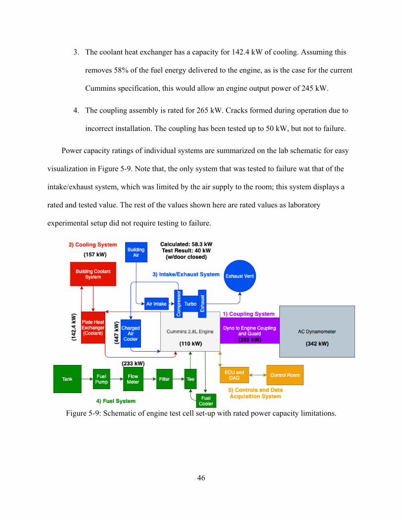
46
3. The coolant heat exchanger has a capacity for 142.4 kW of cooling. Assuming this
removes 58% of the fuel energy delivered to the engine, as is the case for the current
Cummins specification, this would allow an engine output power of 245 kW.
4. The coupling assembly is rated for 265 kW. Cracks formed during operation due to
incorrect installation. The coupling has been tested up to 50 kW, but not to failure.
Power capacity ratings of individual systems are summarized on the lab schematic for easy
visualization in Figure 5-9. Note that, the only system that was tested to failure wat that of the
intake/exhaust system, which was limited by the air supply to the room; this system displays a
rated and tested value. The rest of the values shown here are rated values as laboratory
experimental setup did not require testing to failure.
Figure 5-9: Schematic of engine test cell set-up with rated power capacity limitations.
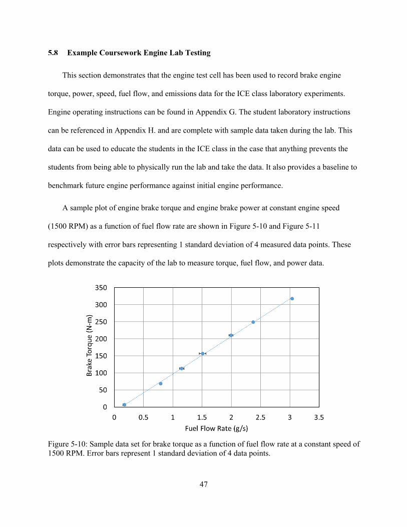
47
Example Coursework Engine Lab Testing
This section demonstrates that the engine test cell has been used to record brake engine
torque, power, speed, fuel flow, and emissions data for the ICE class laboratory experiments.
Engine operating instructions can be found in Appendix G. The student laboratory instructions
can be referenced in Appendix H. and are complete with sample data taken during the lab. This
data can be used to educate the students in the ICE class in the case that anything prevents the
students from being able to physically run the lab and take the data. It also provides a baseline to
benchmark future engine performance against initial engine performance.
A sample plot of engine brake torque and engine brake power at constant engine speed
(1500 RPM) as a function of fuel flow rate are shown in Figure 5-10 and Figure 5-11
respectively with error bars representing 1 standard deviation of 4 measured data points. These
plots demonstrate the capacity of the lab to measure torque, fuel flow, and power data.
Figure 5-10: Sample data set for brake torque as a function of fuel flow rate at a constant speed of 1500 RPM. Error bars represent 1 standard deviation of 4 data points.
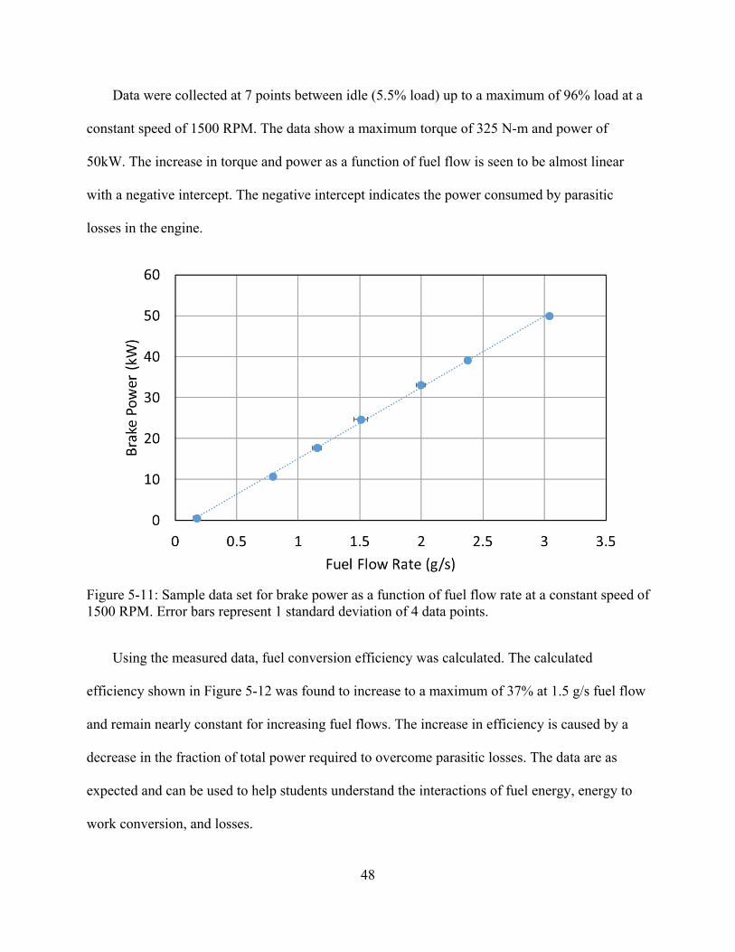
48
Data were collected at 7 points between idle (5.5% load) up to a maximum of 96% load at a
constant speed of 1500 RPM. The data show a maximum torque of 325 N-m and power of
50kW. The increase in torque and power as a function of fuel flow is seen to be almost linear
with a negative intercept. The negative intercept indicates the power consumed by parasitic
losses in the engine.
Figure 5-11: Sample data set for brake power as a function of fuel flow rate at a constant speed of 1500 RPM. Error bars represent 1 standard deviation of 4 data points.
Using the measured data, fuel conversion efficiency was calculated. The calculated
efficiency shown in Figure 5-12 was found to increase to a maximum of 37% at 1.5 g/s fuel flow
and remain nearly constant for increasing fuel flows. The increase in efficiency is caused by a
decrease in the fraction of total power required to overcome parasitic losses. The data are as
expected and can be used to help students understand the interactions of fuel energy, energy to
work conversion, and losses.
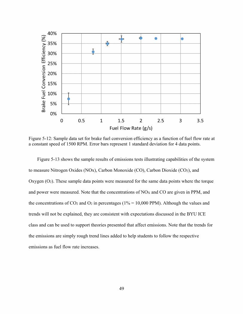
49
Figure 5-12: Sample data set for brake fuel conversion efficiency as a function of fuel flow rate at a constant speed of 1500 RPM. Error bars represent 1 standard deviation for 4 data points.
Figure 5-13 shows the sample results of emissions tests illustrating capabilities of the system
to measure Nitrogen Oxides (NOx), Carbon Monoxide (CO), Carbon Dioxide (CO2), and
Oxygen (O2). These sample data points were measured for the same data points where the torque
and power were measured. Note that the concentrations of NOX and CO are given in PPM, and
the concentrations of CO2 and O2 in percentages (1% = 10,000 PPM). Although the values and
trends will not be explained, they are consistent with expectations discussed in the BYU ICE
class and can be used to support theories presented that affect emissions. Note that the trends for
the emissions are simply rough trend lines added to help students to follow the respective
emissions as fuel flow rate increases.
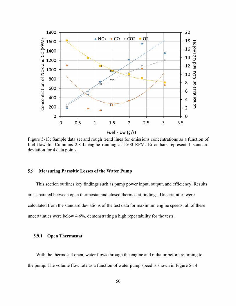
50
Figure 5-13: Sample data set and rough trend lines for emissions concentrations as a function of fuel flow for Cummins 2.8 L engine running at 1500 RPM. Error bars represent 1 standard deviation for 4 data points.
Measuring Parasitic Losses of the Water Pump
This section outlines key findings such as pump power input, output, and efficiency. Results
are separated between open thermostat and closed thermostat findings. Uncertainties were
calculated from the standard deviations of the test data for maximum engine speeds; all of these
uncertainties were below 4.6%, demonstrating a high repeatability for the tests.
5.9.1 Open Thermostat
With the thermostat open, water flows through the engine and radiator before returning to
the pump. The volume flow rate as a function of water pump speed is shown in Figure 5-14.
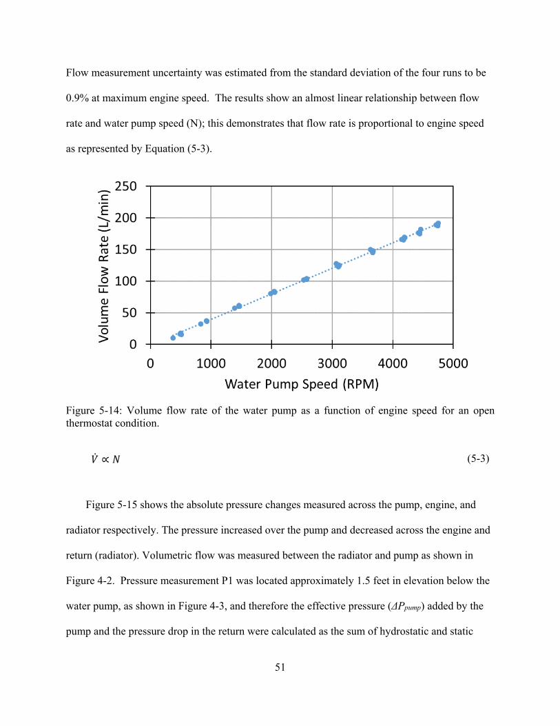
51
Flow measurement uncertainty was estimated from the standard deviation of the four runs to be
0.9% at maximum engine speed. The results show an almost linear relationship between flow
rate and water pump speed (N); this demonstrates that flow rate is proportional to engine speed
as represented by Equation (5-3).
Figure 5-14: Volume flow rate of the water pump as a function of engine speed for an open thermostat condition.
��𝑉 ∝ 𝑁𝑁 (5-3)
Figure 5-15 shows the absolute pressure changes measured across the pump, engine, and
radiator respectively. The pressure increased over the pump and decreased across the engine and
return (radiator). Volumetric flow was measured between the radiator and pump as shown in
Figure 4-2. Pressure measurement P1 was located approximately 1.5 feet in elevation below the
water pump, as shown in Figure 4-3, and therefore the effective pressure (ΔPpump) added by the
pump and the pressure drop in the return were calculated as the sum of hydrostatic and static
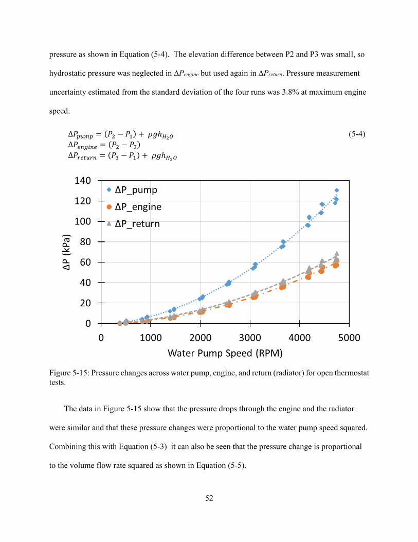
52
pressure as shown in Equation (5-4). The elevation difference between P2 and P3 was small, so
hydrostatic pressure was neglected in ∆Pengine but used again in ∆Preturn. Pressure measurement
uncertainty estimated from the standard deviation of the four runs was 3.8% at maximum engine
speed.
∆𝑃𝑃𝑝𝑝𝑜𝑜𝑝𝑝𝑝𝑝 = (𝑃𝑃2 − 𝑃𝑃1) + 𝜌𝜌𝐸𝐸ℎ𝐻𝐻2𝑂𝑂 ∆𝑃𝑃𝑟𝑟𝑒𝑒𝑒𝑒𝑤𝑤𝑒𝑒𝑟𝑟 = (𝑃𝑃2 − 𝑃𝑃3) ∆𝑃𝑃𝑟𝑟𝑟𝑟𝑤𝑤𝑜𝑜𝑟𝑟𝑒𝑒 = (𝑃𝑃3 − 𝑃𝑃1) + 𝜌𝜌𝐸𝐸ℎ𝐻𝐻2𝑂𝑂
(5-4)
Figure 5-15: Pressure changes across water pump, engine, and return (radiator) for open thermostat tests.
The data in Figure 5-15 show that the pressure drops through the engine and the radiator
were similar and that these pressure changes were proportional to the water pump speed squared.
Combining this with Equation (5-3) it can also be seen that the pressure change is proportional
to the volume flow rate squared as shown in Equation (5-5).
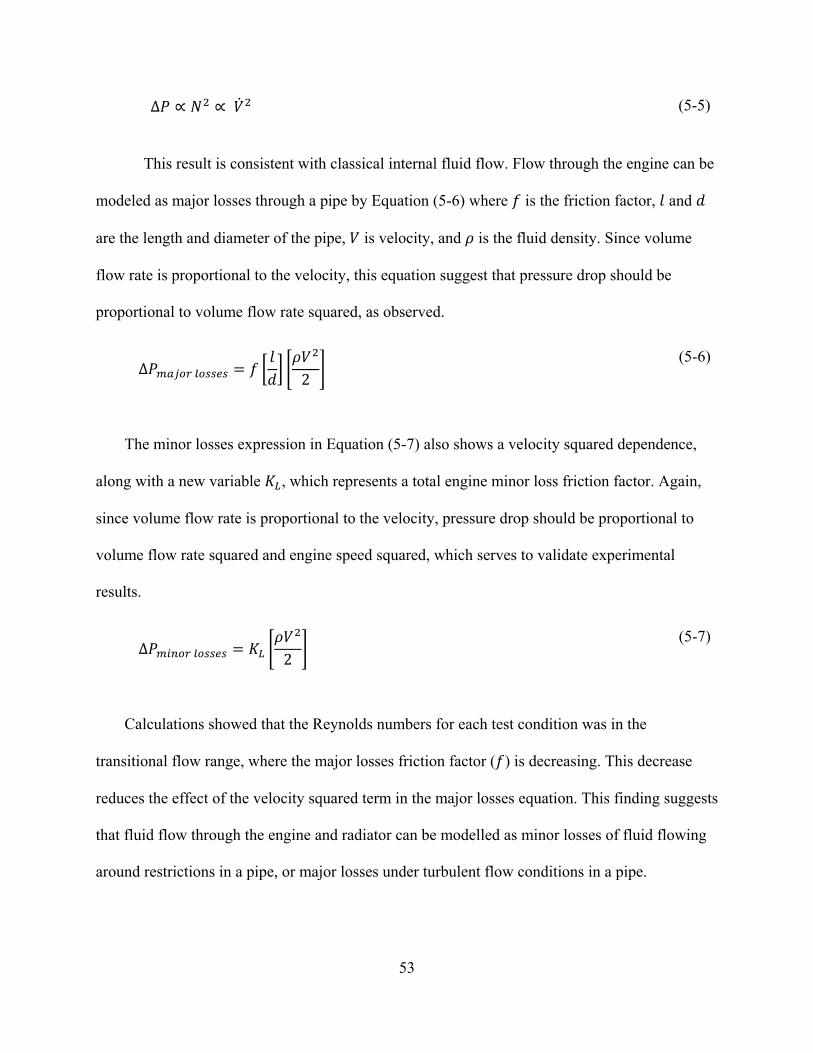
53
∆𝑃𝑃 ∝ 𝑁𝑁2 ∝ ��𝑉2 (5-5)
This result is consistent with classical internal fluid flow. Flow through the engine can be
modeled as major losses through a pipe by Equation (5-6) where 𝑓𝑓 is the friction factor, 𝑙𝑙 and 𝑑𝑑
are the length and diameter of the pipe, 𝑉𝑉 is velocity, and 𝜌𝜌 is the fluid density. Since volume
flow rate is proportional to the velocity, this equation suggest that pressure drop should be
proportional to volume flow rate squared, as observed.
∆𝑃𝑃𝑝𝑝𝑎𝑎𝑚𝑚𝑜𝑜𝑟𝑟 𝑟𝑟𝑜𝑜𝑎𝑎𝑎𝑎𝑟𝑟𝑎𝑎 = 𝑓𝑓 �
𝑙𝑙𝑑𝑑� �𝜌𝜌𝑉𝑉2
2 � (5-6)
The minor losses expression in Equation (5-7) also shows a velocity squared dependence,
along with a new variable 𝐾𝐾𝐿𝐿, which represents a total engine minor loss friction factor. Again,
since volume flow rate is proportional to the velocity, pressure drop should be proportional to
volume flow rate squared and engine speed squared, which serves to validate experimental
results.
∆𝑃𝑃𝑝𝑝𝑤𝑤𝑒𝑒𝑜𝑜𝑟𝑟 𝑟𝑟𝑜𝑜𝑎𝑎𝑎𝑎𝑟𝑟𝑎𝑎 = 𝐾𝐾𝐿𝐿 �
𝜌𝜌𝑉𝑉2
2 � (5-7)
Calculations showed that the Reynolds numbers for each test condition was in the
transitional flow range, where the major losses friction factor (𝑓𝑓) is decreasing. This decrease
reduces the effect of the velocity squared term in the major losses equation. This finding suggests
that fluid flow through the engine and radiator can be modelled as minor losses of fluid flowing
around restrictions in a pipe, or major losses under turbulent flow conditions in a pipe.
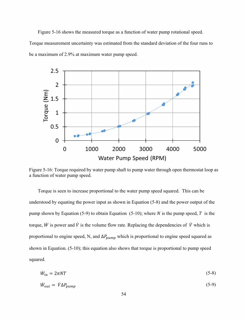
54
Figure 5-16 shows the measured torque as a function of water pump rotational speed.
Torque measurement uncertainty was estimated from the standard deviation of the four runs to
be a maximum of 2.9% at maximum water pump speed.
Figure 5-16: Torque required by water pump shaft to pump water through open thermostat loop as a function of water pump speed.
Torque is seen to increase proportional to the water pump speed squared. This can be
understood by equating the power input as shown in Equation (5-8) and the power output of the
pump shown by Equation (5-9) to obtain Equation (5-10); where 𝑁𝑁 is the pump speed, 𝑇𝑇 is the
torque, ��𝑊 is power and ��𝑉 is the volume flow rate. Replacing the dependencies of ��𝑉 which is
proportional to engine speed, N, and ∆𝑃𝑃𝑝𝑝𝑜𝑜𝑝𝑝𝑝𝑝 which is proportional to engine speed squared as
shown in Equation. (5-10); this equation also shows that torque is proportional to pump speed
squared.
��𝑊𝑤𝑤𝑒𝑒 = 2𝜋𝜋𝑁𝑁𝑇𝑇
(5-8)
��𝑊𝑜𝑜𝑜𝑜𝑤𝑤 = ��𝑉∆𝑃𝑃𝑝𝑝𝑜𝑜𝑝𝑝𝑝𝑝 (5-9)
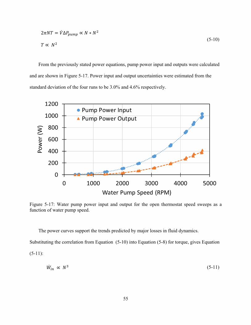
55
2𝜋𝜋𝑁𝑁𝑇𝑇 = ��𝑉∆𝑃𝑃𝑝𝑝𝑜𝑜𝑝𝑝𝑝𝑝 ∝ 𝑁𝑁 ∗ 𝑁𝑁2 𝑇𝑇 ∝ 𝑁𝑁2
(5-10)
From the previously stated power equations, pump power input and outputs were calculated
and are shown in Figure 5-17. Power input and output uncertainties were estimated from the
standard deviation of the four runs to be 3.0% and 4.6% respectively.
Figure 5-17: Water pump power input and output for the open thermostat speed sweeps as a function of water pump speed.
The power curves support the trends predicted by major losses in fluid dynamics.
Substituting the correlation from Equation (5-10) into Equation (5-8) for torque, gives Equation
(5-11):
��𝑊𝑤𝑤𝑒𝑒 ∝ 𝑁𝑁3 (5-11)
56
These findings suggest that for the setup used, fluid flow through the engine and radiator can
be modelled as fluid flowing through a pipe.
The pump efficiency was calculated with Equation (5-12), and a plot of efficiency as a
function of pump speed is shown in Figure 5-18. The pump efficiency is near zero at low speeds
and increases until it asymptotes at 38% above pump speeds of 3500 RPM. This shows that the
pump spins at low speed without flowing any fluid, perhaps due to the need to overcome
hydrostatic forces. Once water is flowing, the mechanical friction and hydrostatic forces become
a smaller fraction of the total force required, and the pump losses become a constant fraction of
the total power at high speed.
𝜂𝜂 =
��𝑊𝑜𝑜𝑜𝑜𝑤𝑤
��𝑊𝑤𝑤𝑒𝑒
(5-12)
Figure 5-18: Water pump efficiency as a function of water pump speed for the open thermostat water pump speed sweeps.
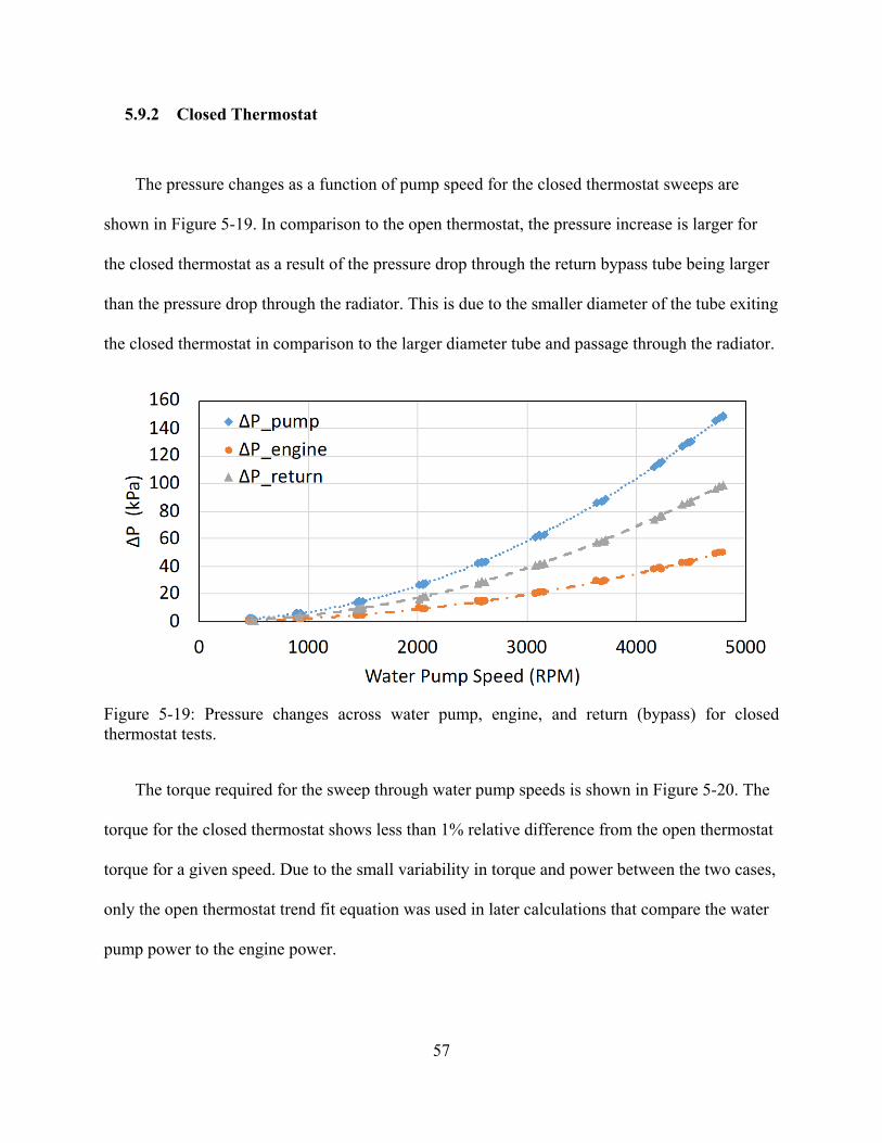
57
5.9.2 Closed Thermostat
The pressure changes as a function of pump speed for the closed thermostat sweeps are
shown in Figure 5-19. In comparison to the open thermostat, the pressure increase is larger for
the closed thermostat as a result of the pressure drop through the return bypass tube being larger
than the pressure drop through the radiator. This is due to the smaller diameter of the tube exiting
the closed thermostat in comparison to the larger diameter tube and passage through the radiator.
Figure 5-19: Pressure changes across water pump, engine, and return (bypass) for closed thermostat tests.
The torque required for the sweep through water pump speeds is shown in Figure 5-20. The
torque for the closed thermostat shows less than 1% relative difference from the open thermostat
torque for a given speed. Due to the small variability in torque and power between the two cases,
only the open thermostat trend fit equation was used in later calculations that compare the water
pump power to the engine power.
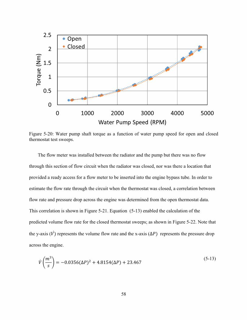
58
Figure 5-20: Water pump shaft torque as a function of water pump speed for open and closed thermostat test sweeps.
The flow meter was installed between the radiator and the pump but there was no flow
through this section of flow circuit when the radiator was closed, nor was there a location that
provided a ready access for a flow meter to be inserted into the engine bypass tube. In order to
estimate the flow rate through the circuit when the thermostat was closed, a correlation between
flow rate and pressure drop across the engine was determined from the open thermostat data.
This correlation is shown in Figure 5-21. Equation (5-13) enabled the calculation of the
predicted volume flow rate for the closed thermostat sweeps; as shown in Figure 5-22. Note that
the y-axis (𝑉𝑉) represents the volume flow rate and the x-axis (∆𝑃𝑃) represents the pressure drop
across the engine.
��𝑉 �
𝑚𝑚3
𝑠𝑠� = −0.0356(∆𝑃𝑃)2 + 4.8154(∆𝑃𝑃) + 23.467
(5-13)
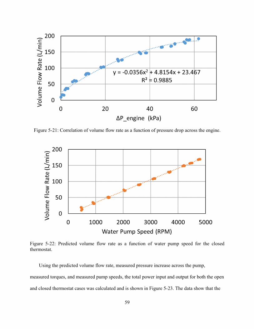
59
Figure 5-21: Correlation of volume flow rate as a function of pressure drop across the engine.
Figure 5-22: Predicted volume flow rate as a function of water pump speed for the closed thermostat.
Using the predicted volume flow rate, measured pressure increase across the pump,
measured torques, and measured pump speeds, the total power input and output for both the open
and closed thermostat cases was calculated and is shown in Figure 5-23. The data show that the
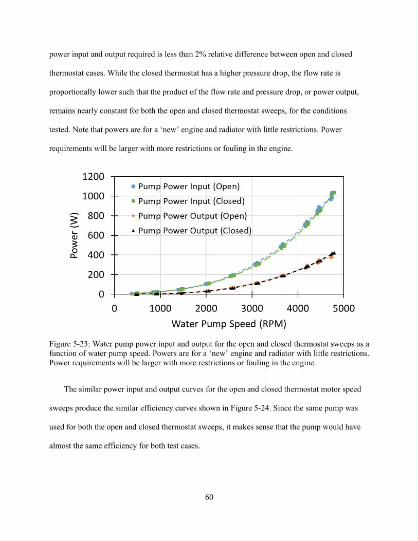
60
power input and output required is less than 2% relative difference between open and closed
thermostat cases. While the closed thermostat has a higher pressure drop, the flow rate is
proportionally lower such that the product of the flow rate and pressure drop, or power output,
remains nearly constant for both the open and closed thermostat sweeps, for the conditions
tested. Note that powers are for a ‘new’ engine and radiator with little restrictions. Power
requirements will be larger with more restrictions or fouling in the engine.
Figure 5-23: Water pump power input and output for the open and closed thermostat sweeps as a function of water pump speed. Powers are for a ‘new’ engine and radiator with little restrictions. Power requirements will be larger with more restrictions or fouling in the engine.
The similar power input and output curves for the open and closed thermostat motor speed
sweeps produce the similar efficiency curves shown in Figure 5-24. Since the same pump was
used for both the open and closed thermostat sweeps, it makes sense that the pump would have
almost the same efficiency for both test cases.
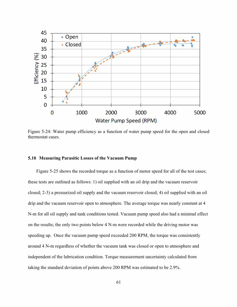
61
Figure 5-24: Water pump efficiency as a function of water pump speed for the open and closed thermostat cases.
Measuring Parasitic Losses of the Vacuum Pump
Figure 5-25 shows the recorded torque as a function of motor speed for all of the test cases;
these tests are outlined as follows: 1) oil supplied with an oil drip and the vacuum reservoir
closed; 2-3) a pressurized oil supply and the vacuum reservoir closed; 4) oil supplied with an oil
drip and the vacuum reservoir open to atmosphere. The average torque was nearly constant at 4
N-m for all oil supply and tank conditions tested. Vacuum pump speed also had a minimal effect
on the results; the only two points below 4 N-m were recorded while the driving motor was
speeding up. Once the vacuum pump speed exceeded 200 RPM, the torque was consistently
around 4 N-m regardless of whether the vacuum tank was closed or open to atmosphere and
independent of the lubrication condition. Torque measurement uncertainty calculated from
taking the standard deviation of points above 200 RPM was estimated to be 2.9%.
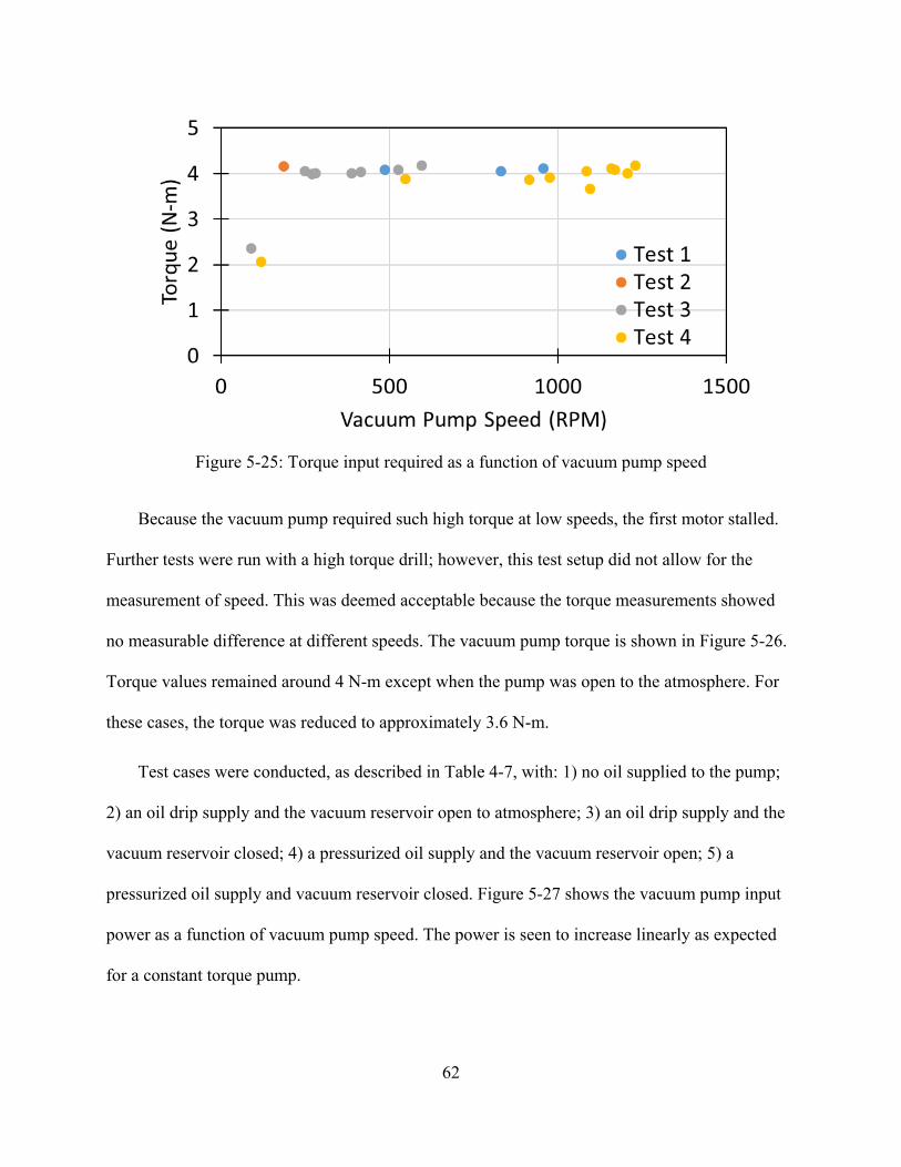
62
Figure 5-25: Torque input required as a function of vacuum pump speed
Because the vacuum pump required such high torque at low speeds, the first motor stalled.
Further tests were run with a high torque drill; however, this test setup did not allow for the
measurement of speed. This was deemed acceptable because the torque measurements showed
no measurable difference at different speeds. The vacuum pump torque is shown in Figure 5-26.
Torque values remained around 4 N-m except when the pump was open to the atmosphere. For
these cases, the torque was reduced to approximately 3.6 N-m.
Test cases were conducted, as described in Table 4-7, with: 1) no oil supplied to the pump;
2) an oil drip supply and the vacuum reservoir open to atmosphere; 3) an oil drip supply and the
vacuum reservoir closed; 4) a pressurized oil supply and the vacuum reservoir open; 5) a
pressurized oil supply and vacuum reservoir closed. Figure 5-27 shows the vacuum pump input
power as a function of vacuum pump speed. The power is seen to increase linearly as expected
for a constant torque pump.
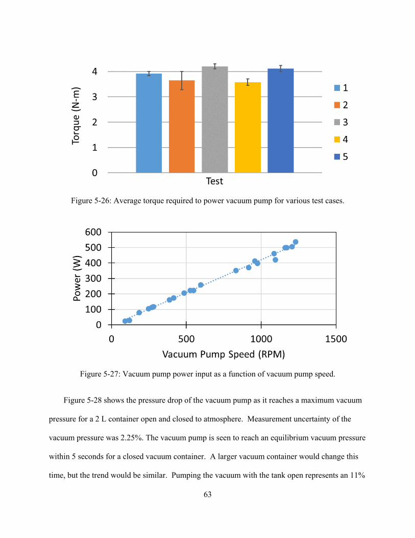
63
Figure 5-26: Average torque required to power vacuum pump for various test cases.
Figure 5-27: Vacuum pump power input as a function of vacuum pump speed.
Figure 5-28 shows the pressure drop of the vacuum pump as it reaches a maximum vacuum
pressure for a 2 L container open and closed to atmosphere. Measurement uncertainty of the
vacuum pressure was 2.25%. The vacuum pump is seen to reach an equilibrium vacuum pressure
within 5 seconds for a closed vacuum container. A larger vacuum container would change this
time, but the trend would be similar. Pumping the vacuum with the tank open represents an 11%
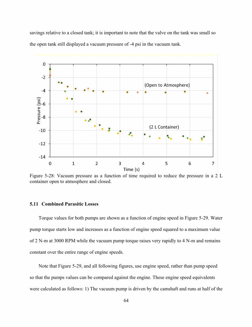
64
savings relative to a closed tank; it is important to note that the valve on the tank was small so
the open tank still displayed a vacuum pressure of -4 psi in the vacuum tank.
Figure 5-28: Vacuum pressure as a function of time required to reduce the pressure in a 2 L container open to atmosphere and closed.
Combined Parasitic Losses
Torque values for both pumps are shown as a function of engine speed in Figure 5-29. Water
pump torque starts low and increases as a function of engine speed squared to a maximum value
of 2 N-m at 3000 RPM while the vacuum pump torque raises very rapidly to 4 N-m and remains
constant over the entire range of engine speeds.
Note that Figure 5-29, and all following figures, use engine speed, rather than pump speed
so that the pumps values can be compared against the engine. These engine speed equivalents
were calculated as follows: 1) The vacuum pump is driven by the camshaft and runs at half of the
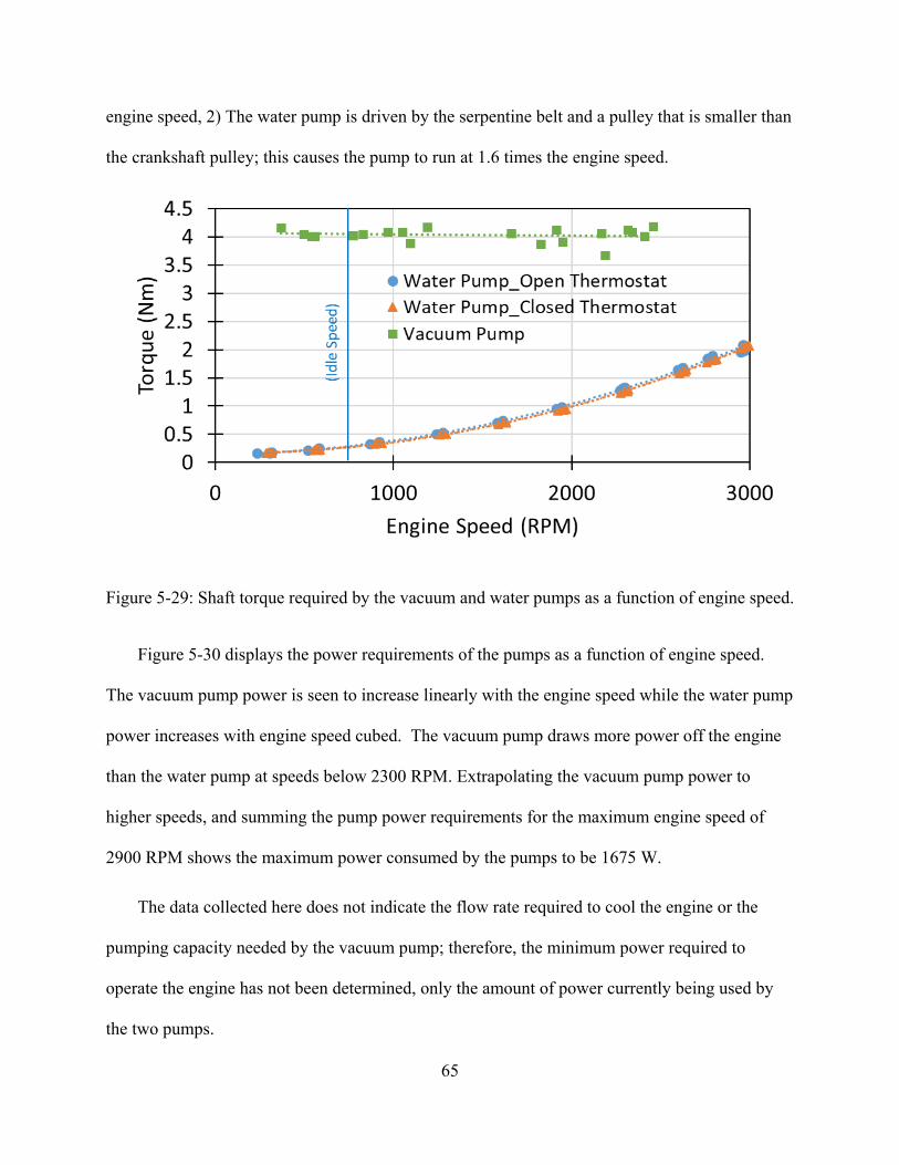
65
engine speed, 2) The water pump is driven by the serpentine belt and a pulley that is smaller than
the crankshaft pulley; this causes the pump to run at 1.6 times the engine speed.
Figure 5-29: Shaft torque required by the vacuum and water pumps as a function of engine speed.
Figure 5-30 displays the power requirements of the pumps as a function of engine speed.
The vacuum pump power is seen to increase linearly with the engine speed while the water pump
power increases with engine speed cubed. The vacuum pump draws more power off the engine
than the water pump at speeds below 2300 RPM. Extrapolating the vacuum pump power to
higher speeds, and summing the pump power requirements for the maximum engine speed of
2900 RPM shows the maximum power consumed by the pumps to be 1675 W.
The data collected here does not indicate the flow rate required to cool the engine or the
pumping capacity needed by the vacuum pump; therefore, the minimum power required to
operate the engine has not been determined, only the amount of power currently being used by
the two pumps.
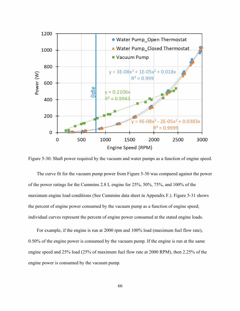
66
Figure 5-30: Shaft power required by the vacuum and water pumps as a function of engine speed.
The curve fit for the vacuum pump power from Figure 5-30 was compared against the power
of the power ratings for the Cummins 2.8 L engine for 25%, 50%, 75%, and 100% of the
maximum engine load conditions (See Cummins data sheet in Appendix F.). Figure 5-31 shows
the percent of engine power consumed by the vacuum pump as a function of engine speed;
individual curves represent the percent of engine power consumed at the stated engine loads.
For example, if the engine is run at 2000 rpm and 100% load (maximum fuel flow rate),
0.50% of the engine power is consumed by the vacuum pump. If the engine is run at the same
engine speed and 25% load (25% of maximum fuel flow rate at 2000 RPM), then 2.25% of the
engine power is consumed by the vacuum pump.
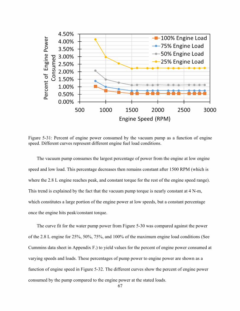
67
Figure 5-31: Percent of engine power consumed by the vacuum pump as a function of engine speed. Different curves represent different engine fuel load conditions.
The vacuum pump consumes the largest percentage of power from the engine at low engine
speed and low load. This percentage decreases then remains constant after 1500 RPM (which is
where the 2.8 L engine reaches peak, and constant torque for the rest of the engine speed range).
This trend is explained by the fact that the vacuum pump torque is nearly constant at 4 N-m,
which constitutes a large portion of the engine power at low speeds, but a constant percentage
once the engine hits peak/constant torque.
The curve fit for the water pump power from Figure 5-30 was compared against the power
of the 2.8 L engine for 25%, 50%, 75%, and 100% of the maximum engine load conditions (See
Cummins data sheet in Appendix F.) to yield values for the percent of engine power consumed at
varying speeds and loads. These percentages of pump power to engine power are shown as a
function of engine speed in Figure 5-32. The different curves show the percent of engine power
consumed by the pump compared to the engine power at the stated loads.
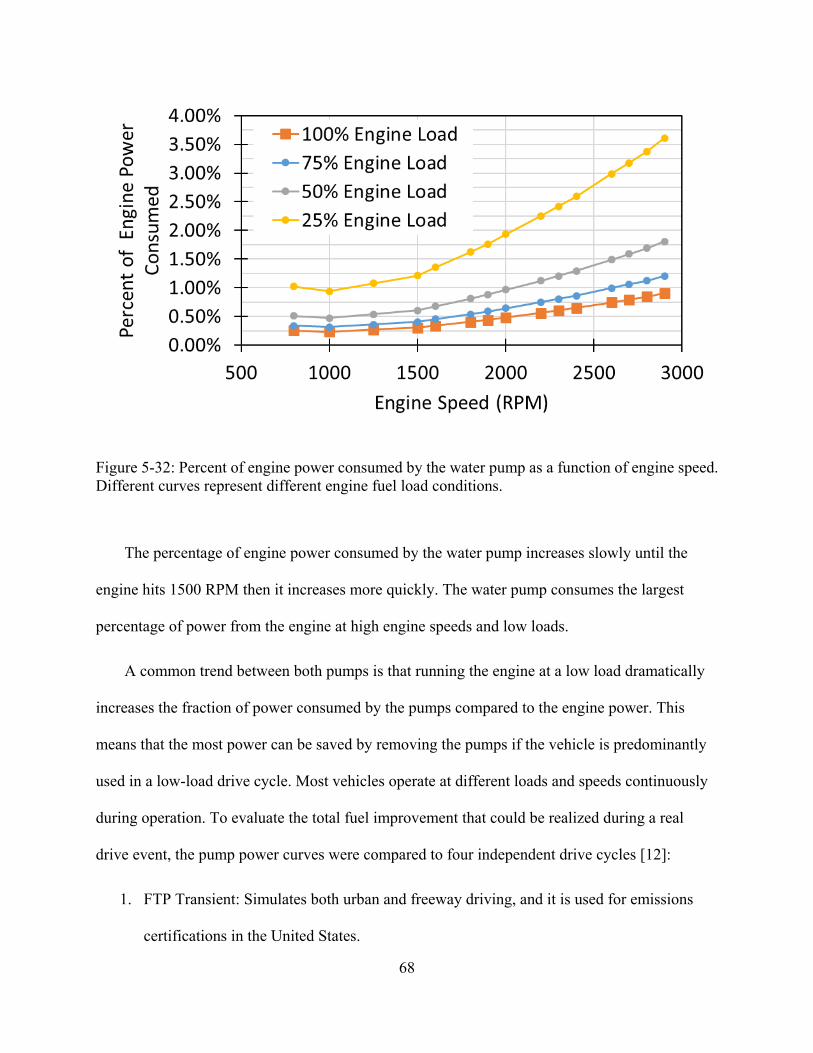
68
Figure 5-32: Percent of engine power consumed by the water pump as a function of engine speed. Different curves represent different engine fuel load conditions.
The percentage of engine power consumed by the water pump increases slowly until the
engine hits 1500 RPM then it increases more quickly. The water pump consumes the largest
percentage of power from the engine at high engine speeds and low loads.
A common trend between both pumps is that running the engine at a low load dramatically
increases the fraction of power consumed by the pumps compared to the engine power. This
means that the most power can be saved by removing the pumps if the vehicle is predominantly
used in a low-load drive cycle. Most vehicles operate at different loads and speeds continuously
during operation. To evaluate the total fuel improvement that could be realized during a real
drive event, the pump power curves were compared to four independent drive cycles [12]:
1. FTP Transient: Simulates both urban and freeway driving, and it is used for emissions
certifications in the United States.
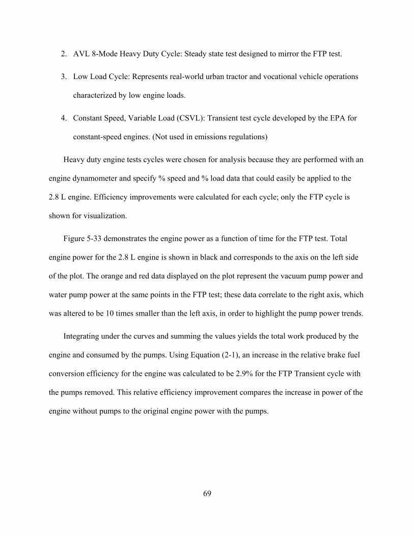
69
2. AVL 8-Mode Heavy Duty Cycle: Steady state test designed to mirror the FTP test.
3. Low Load Cycle: Represents real-world urban tractor and vocational vehicle operations
characterized by low engine loads.
4. Constant Speed, Variable Load (CSVL): Transient test cycle developed by the EPA for
constant-speed engines. (Not used in emissions regulations)
Heavy duty engine tests cycles were chosen for analysis because they are performed with an
engine dynamometer and specify % speed and % load data that could easily be applied to the
2.8 L engine. Efficiency improvements were calculated for each cycle; only the FTP cycle is
shown for visualization.
Figure 5-33 demonstrates the engine power as a function of time for the FTP test. Total
engine power for the 2.8 L engine is shown in black and corresponds to the axis on the left side
of the plot. The orange and red data displayed on the plot represent the vacuum pump power and
water pump power at the same points in the FTP test; these data correlate to the right axis, which
was altered to be 10 times smaller than the left axis, in order to highlight the pump power trends.
Integrating under the curves and summing the values yields the total work produced by the
engine and consumed by the pumps. Using Equation (2-1), an increase in the relative brake fuel
conversion efficiency for the engine was calculated to be 2.9% for the FTP Transient cycle with
the pumps removed. This relative efficiency improvement compares the increase in power of the
engine without pumps to the original engine power with the pumps.
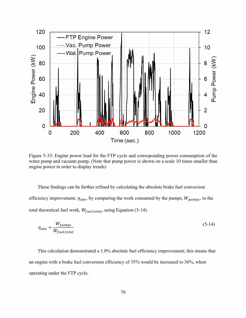
70
Figure 5-33: Engine power load for the FTP cycle and corresponding power consumption of the water pump and vacuum pump. (Note that pump power is shown on a scale 10 times smaller than engine power in order to display trends)
These findings can be further refined by calculating the absolute brake fuel conversion
efficiency improvement, 𝜂𝜂𝑎𝑎𝑎𝑎𝑎𝑎, by comparing the work consumed by the pumps, 𝑊𝑊 𝑝𝑝𝑜𝑜𝑝𝑝𝑝𝑝𝑎𝑎, to the
total theoretical fuel work, 𝑊𝑊𝑓𝑓𝑜𝑜𝑟𝑟𝑟𝑟,𝑤𝑤𝑜𝑜𝑤𝑤𝑎𝑎𝑟𝑟, using Equation (5-14).
𝜂𝜂𝑎𝑎𝑎𝑎𝑎𝑎 = 𝑊𝑊 𝑝𝑝𝑜𝑜𝑝𝑝𝑝𝑝𝑎𝑎 𝑊𝑊𝑓𝑓𝑜𝑜𝑟𝑟𝑟𝑟,𝑤𝑤𝑜𝑜𝑤𝑤𝑎𝑎𝑟𝑟
(5-14)
This calculation demonstrated a 1.0% absolute fuel efficiency improvement; this means that
an engine with a brake fuel conversion efficiency of 35% would be increased to 36%, when
operating under the FTP cycle.
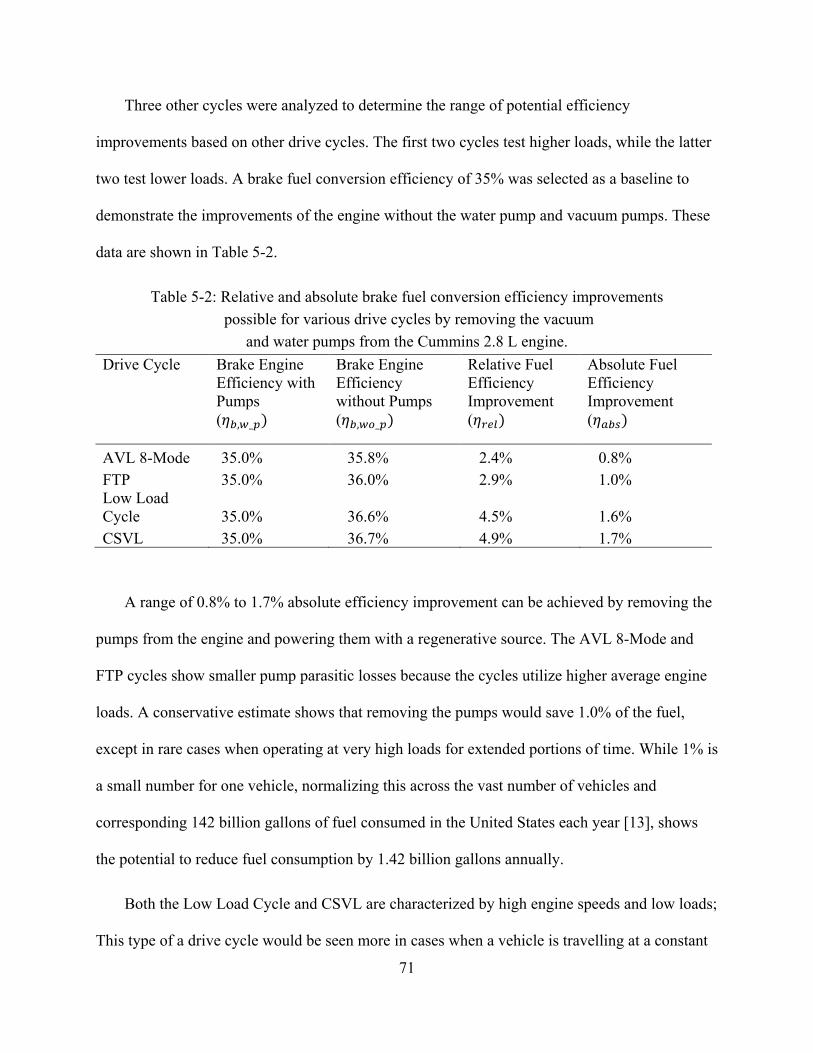
71
Three other cycles were analyzed to determine the range of potential efficiency
improvements based on other drive cycles. The first two cycles test higher loads, while the latter
two test lower loads. A brake fuel conversion efficiency of 35% was selected as a baseline to
demonstrate the improvements of the engine without the water pump and vacuum pumps. These
data are shown in Table 5-2.
Table 5-2: Relative and absolute brake fuel conversion efficiency improvements possible for various drive cycles by removing the vacuum
and water pumps from the Cummins 2.8 L engine. Drive Cycle Brake Engine
Efficiency with Pumps (𝜂𝜂𝑎𝑎,𝑤𝑤_𝑝𝑝)
Brake Engine Efficiency without Pumps (𝜂𝜂𝑎𝑎,𝑤𝑤𝑜𝑜_𝑝𝑝)
Relative Fuel Efficiency Improvement (𝜂𝜂𝑟𝑟𝑟𝑟𝑟𝑟)
Absolute Fuel Efficiency Improvement (𝜂𝜂𝑎𝑎𝑎𝑎𝑎𝑎)
AVL 8-Mode 35.0% 35.8% 2.4% 0.8% FTP 35.0% 36.0% 2.9% 1.0% Low Load Cycle 35.0% 36.6% 4.5% 1.6% CSVL 35.0% 36.7% 4.9% 1.7%
A range of 0.8% to 1.7% absolute efficiency improvement can be achieved by removing the
pumps from the engine and powering them with a regenerative source. The AVL 8-Mode and
FTP cycles show smaller pump parasitic losses because the cycles utilize higher average engine
loads. A conservative estimate shows that removing the pumps would save 1.0% of the fuel,
except in rare cases when operating at very high loads for extended portions of time. While 1% is
a small number for one vehicle, normalizing this across the vast number of vehicles and
corresponding 142 billion gallons of fuel consumed in the United States each year [13], shows
the potential to reduce fuel consumption by 1.42 billion gallons annually.
Both the Low Load Cycle and CSVL are characterized by high engine speeds and low loads;
This type of a drive cycle would be seen more in cases when a vehicle is travelling at a constant
72
speed and low load the majority of the time as opposed to the more stop-and-go FTP and AVL 8-
Mode drive cycles. Lower load cycles showed the potential to increase absolute brake fuel
conversion efficiency by up to 1.7%. This is more than a 0.5% increase over the other drive
cycles. This demonstrates that removing the pumps will make a larger difference for vehicles
that normally operate at low loads. One optimal application might be long-haul semi-tractor
trailer trucks that travel large distances each year on the freeway.
The real world implications of these results can be demonstrated by applying the FTP 2.9%
relative efficiency improvement (which correlates to a 1% absolute efficiency improvement) to a
car that currently achieves 33 mpg. The resulting fuel economy with the vacuum pump and water
pump removed (powered by a regenerative source such as exhaust or braking) would be 34 mpg.
Repeating this calculation for the same vehicle on the Low Load Cycle would yield a 34.5 mpg
vehicle.
73
6 SUMMARY AND CONCLUSIONS
A diesel engine test cell has been commissioned with a Cummins 2.8 L diesel engine
connected to an AC motoring dynamometer. The auxiliary coupling, cooling, intake and exhaust,
fuel, and controls/data acquisitions systems are fully operational. Power ratings of key
components are outlined in Figure 5-9 and Table 5-1; the test cell has been demonstrated on the
2.8 L diesel engine up to a brake power of 50 kW, and is designed to run the current engine at
110 kW. The bill of materials, applicable drawings, and wiring diagrams can be referenced in the
Appendices.
The test cell has been used for ICE class instructional labs that measure brake engine speed,
torque, power, fuel consumption, and emissions. Diesel engine operating instructions have been
developed, tested, and are included in Appendix G. Additionally, laboratory instructions have
been developed and used to run two separate lab experiments for 40 students. The laboratory
instructions are included in Appendix H. and are complete with sample data taken from the labs.
This data can be used in the future in the case that the lab cannot be physically run; it can also be
used to benchmark future engine performance against initial operating performance.
The parasitic losses of the vacuum pump and water pump have been measured. These results
have been analyzed to reveal power trends for the respective pumps. The respective pump
parasitic power requirements have been compared against various drive cycles to understand the
overall potential improvement in brake fuel conversion efficiency of the engine by removing the
pumps. Conclusions from the parasitic loss results are as follows:
1. The water pump torque increases proportional to engine speed squared. This finding
suggests that fluid flow through the engine and radiator can be modelled as minor losses
74
of fluid flowing around restrictions in a pipe, or major losses under turbulent flow
conditions in a pipe. Water pump power consumption increases proportional to engine
speed cubed.
2. Vacuum pump torque was measured and found to be nearly constant at 4 N-m for all
vacuum pump conditions tested. The vacuum pump power consumption increases
linearly with engine speed.
3. The percent power consumed by the pumps with regards to engine power has been
demonstrated for various engine loads and speeds. (See Figure 5-31 and Figure 5-32)
4. Finally, pump power consumption has been applied to 4 heavy duty engine drive cycles
and relative and absolute fuel conversion efficiencies have been calculated. Relative
brake fuel conversion efficiency improvements possible by removing both pumps range
from 2.4% to 4.9%. Absolute brake fuel conversion efficiency improvements possible by
removing both pumps range from 0.8% to 1.7%. Efficiency improvements are
maximized for vehicles operating at low engine loads and high engine speeds.
75
REFERENCES
[1] EPA, NHTSA, "2017 and Later Model Year Light-Duty Vehicle Greenhouse Gas Emissions and Corporate Average Fuel Economy Standards"," Federal Register, 2010.
[2] Government, "Federal Register 06576," 2017.
[3] CNBC, "Trump Administration rolls back plans to raise fuel economy standards," 02 08 2018. [Online]. Available: https://www.cnbc.com/2018/08/02/trump-administration-rolls-back-plans-to-raise-fuel-economy-standards.html .
[4] F. Economy.gov, "fueleconomy.gov," [Online]. Available: https://www.fueleconomy.gov/feg/atv.shtml. [Accessed 2020].
[5] J. P. R. Shutty, "Advanced Thermal Management Strategies," SAE, vol. 36, no. Fig 19, p. 542, 2013.
[6] R. A. D. Chalgren, "Light Duty Diesel Advanced Thermal Management," SAE Intl., vol. 01, p. 2020, 2005.
[7] R. M. S. N. R. Babu, "Electrical Operated Fan for Cooling System on Agricultural Tractors," SAE International, vol. 26, p. 0079, 2019.
[8] M. D. B. K. Y. Lyu, "A Study of Vehicle Fuel Economy Improvement Potential by Optimization of the Cooling and Ancillary Systems of a Heavy Duty Engine," SAE International, vol. 01, p. 1772, 2007.
[9] D. M. J. Bitsis, "Optimization of Heavy Duty Diesel Engine Lubricant and Coolant Pumps for Parasitic Loss Reduction," SAE International, vol. 01, p. 0980, 2018.
[10] N. Anandakumaran, "Development of an Electrcally Operated Vacuum Pump," SAE International, vol. 28, p. 1772, 2007.
[11] D. Scopacasa, "Effects of Supplemental Vacuum Production to Support Pump," SAE International, vol. 01, p. 2528, 2014.
[12] DieselNet, "Dieselnet.com," [Online]. Available: https://dieselnet.com/standards/cycles/index.php#us-hden. [Accessed 2020].
[13] E. I. Administration, "eia.gov," [Online]. Available: https://www.eia.gov/tools/faqs/faq.php?id=23&t=10.
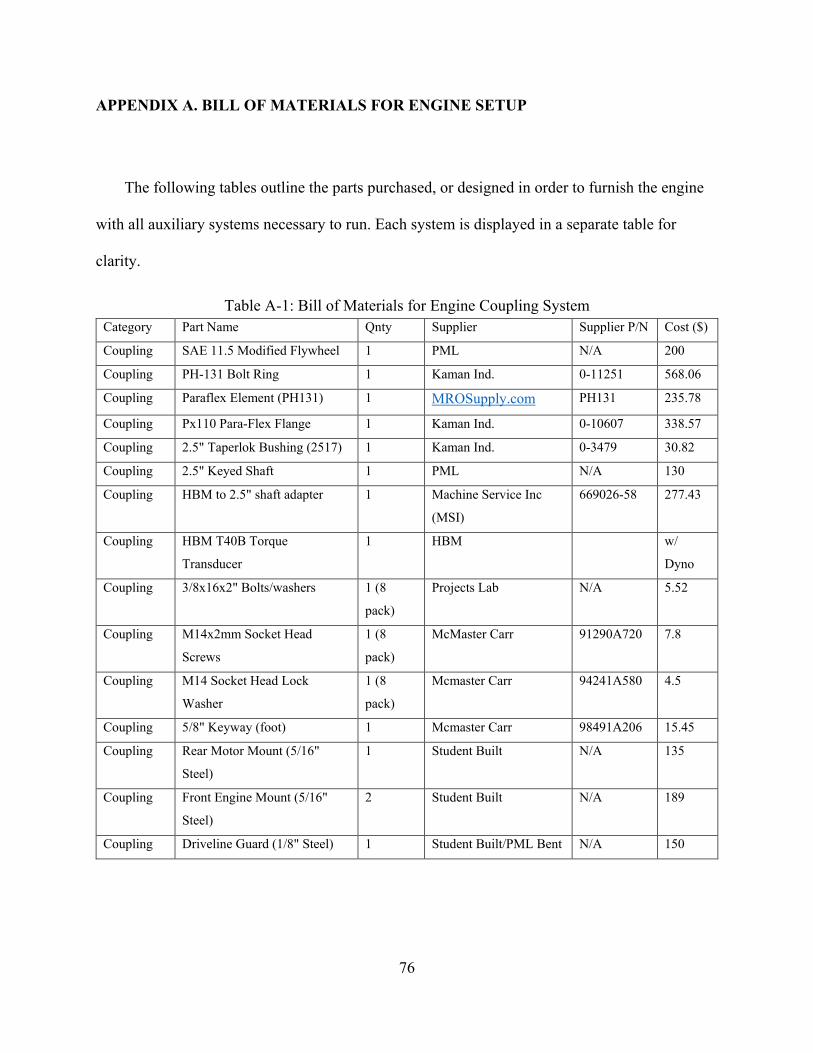
76
APPENDIX A. BILL OF MATERIALS FOR ENGINE SETUP
The following tables outline the parts purchased, or designed in order to furnish the engine
with all auxiliary systems necessary to run. Each system is displayed in a separate table for
clarity.
Table A-1: Bill of Materials for Engine Coupling System Category Part Name Qnty Supplier Supplier P/N Cost ($)
Coupling SAE 11.5 Modified Flywheel 1 PML N/A 200
Coupling PH-131 Bolt Ring 1 Kaman Ind. 0-11251 568.06
Coupling Paraflex Element (PH131) 1 MROSupply.com
PH131 235.78
Coupling Px110 Para-Flex Flange 1 Kaman Ind. 0-10607 338.57
Coupling 2.5" Taperlok Bushing (2517) 1 Kaman Ind. 0-3479 30.82
Coupling 2.5" Keyed Shaft 1 PML N/A 130
Coupling HBM to 2.5" shaft adapter 1 Machine Service Inc
(MSI)
669026-58 277.43
Coupling HBM T40B Torque
Transducer
1 HBM
w/
Dyno
Coupling 3/8x16x2" Bolts/washers 1 (8
pack)
Projects Lab N/A 5.52
Coupling M14x2mm Socket Head
Screws
1 (8
pack)
McMaster Carr 91290A720 7.8
Coupling M14 Socket Head Lock
Washer
1 (8
pack)
Mcmaster Carr 94241A580 4.5
Coupling 5/8" Keyway (foot) 1 Mcmaster Carr 98491A206 15.45
Coupling Rear Motor Mount (5/16"
Steel)
1 Student Built N/A 135
Coupling Front Engine Mount (5/16"
Steel)
2 Student Built N/A 189
Coupling Driveline Guard (1/8" Steel) 1 Student Built/PML Bent N/A 150
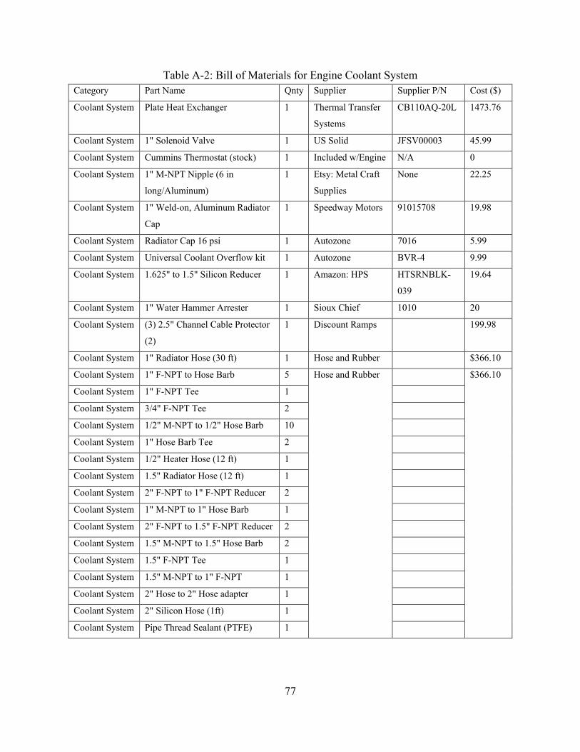
77
Table A-2: Bill of Materials for Engine Coolant System Category Part Name Qnty Supplier Supplier P/N Cost ($)
Coolant System Plate Heat Exchanger 1 Thermal Transfer
Systems
CB110AQ-20L 1473.76
Coolant System 1" Solenoid Valve 1 US Solid JFSV00003 45.99
Coolant System Cummins Thermostat (stock) 1 Included w/Engine N/A 0
Coolant System 1" M-NPT Nipple (6 in
long/Aluminum)
1 Etsy: Metal Craft
Supplies
None 22.25
Coolant System 1" Weld-on, Aluminum Radiator
Cap
1 Speedway Motors 91015708 19.98
Coolant System Radiator Cap 16 psi 1 Autozone 7016 5.99
Coolant System Universal Coolant Overflow kit 1 Autozone BVR-4 9.99
Coolant System 1.625" to 1.5" Silicon Reducer 1 Amazon: HPS HTSRNBLK-
039
19.64
Coolant System 1" Water Hammer Arrester 1 Sioux Chief 1010 20
Coolant System (3) 2.5" Channel Cable Protector
(2)
1 Discount Ramps 199.98
Coolant System 1" Radiator Hose (30 ft) 1 Hose and Rubber $366.10
Coolant System 1" F-NPT to Hose Barb 5 Hose and Rubber $366.10
Coolant System 1" F-NPT Tee 1 Coolant System 3/4" F-NPT Tee 2 Coolant System 1/2" M-NPT to 1/2" Hose Barb 10 Coolant System 1" Hose Barb Tee 2 Coolant System 1/2" Heater Hose (12 ft) 1 Coolant System 1.5" Radiator Hose (12 ft) 1 Coolant System 2" F-NPT to 1" F-NPT Reducer 2 Coolant System 1" M-NPT to 1" Hose Barb 1 Coolant System 2" F-NPT to 1.5" F-NPT Reducer 2 Coolant System 1.5" M-NPT to 1.5" Hose Barb 2 Coolant System 1.5" F-NPT Tee 1 Coolant System 1.5" M-NPT to 1" F-NPT 1 Coolant System 2" Hose to 2" Hose adapter 1 Coolant System 2" Silicon Hose (1ft) 1 Coolant System Pipe Thread Sealant (PTFE) 1
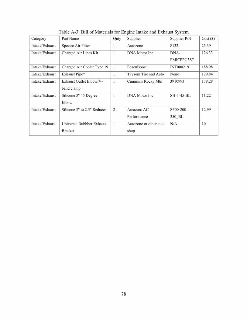
78
Table A-3: Bill of Materials for Engine Intake and Exhaust System Category Part Name Qnty Supplier Supplier P/N Cost ($)
Intake/Exhaust Spectre Air Filter 1 Autozone 8132 25.39
Intake/Exhaust Charged Air Lines Kit 1 DNA Motor Inc DNA-
FMICPPU3ST
126.33
Intake/Exhaust Charged Air Cooler Type 19 1 FozenBoost INT000219 188.98
Intake/Exhaust Exhaust Pipe* 1 Taysom Tire and Auto None 129.84
Intake/Exhaust Exhaust Outlet Elbow/V-
band clamp
1 Cummins Rocky Mtn 3910993 178.28
Intake/Exhaust Silicone 3" 45 Degree
Elbow
1 DNA Motor Inc SH-3-45-BL 11.22
Intake/Exhaust Silicone 3" to 2.5" Reducer 2 Amazon: AC
Performance
SP00-200-
250_BL
12.99
Intake/Exhaust Universal Rubbber Exhaust
Bracket
1 Autozone or other auto
shop
N/A 10
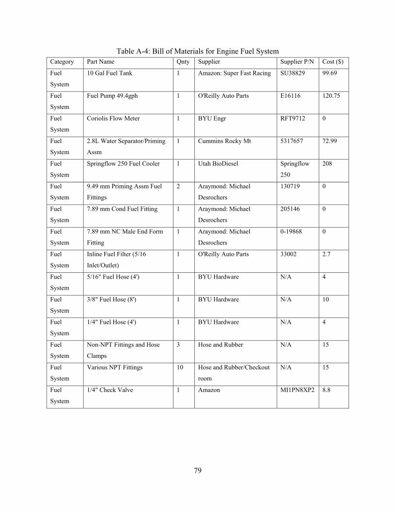
79
Table A-4: Bill of Materials for Engine Fuel System Category Part Name Qnty Supplier Supplier P/N Cost ($)
Fuel
System
10 Gal Fuel Tank 1 Amazon: Super Fast Racing SU38829 99.69
Fuel
System
Fuel Pump 49.4gph 1 O'Reilly Auto Parts E16116 120.75
Fuel
System
Coriolis Flow Meter 1 BYU Engr RFT9712 0
Fuel
System
2.8L Water Separator/Priming
Assm
1 Cummins Rocky Mt 5317657 72.99
Fuel
System
Springflow 250 Fuel Cooler 1 Utah BioDiesel Springflow
250
208
Fuel
System
9.49 mm Priming Assm Fuel
Fittings
2 Araymond: Michael
Desrochers
130719 0
Fuel
System
7.89 mm Cond Fuel Fitting 1 Araymond: Michael
Desrochers
205146 0
Fuel
System
7.89 mm NC Male End Form
Fitting
1 Araymond: Michael
Desrochers
0-19868 0
Fuel
System
Inline Fuel Filter (5/16
Inlet/Outlet)
1 O'Reilly Auto Parts 33002 2.7
Fuel
System
5/16" Fuel Hose (4') 1 BYU Hardware N/A 4
Fuel
System
3/8" Fuel Hose (8') 1 BYU Hardware N/A 10
Fuel
System
1/4" Fuel Hose (4') 1 BYU Hardware N/A 4
Fuel
System
Non-NPT Fittings and Hose
Clamps
3 Hose and Rubber N/A 15
Fuel
System
Various NPT Fittings 10 Hose and Rubber/Checkout
room
N/A 15
Fuel
System
1/4" Check Valve 1 Amazon MI1PN8XP2 8.8
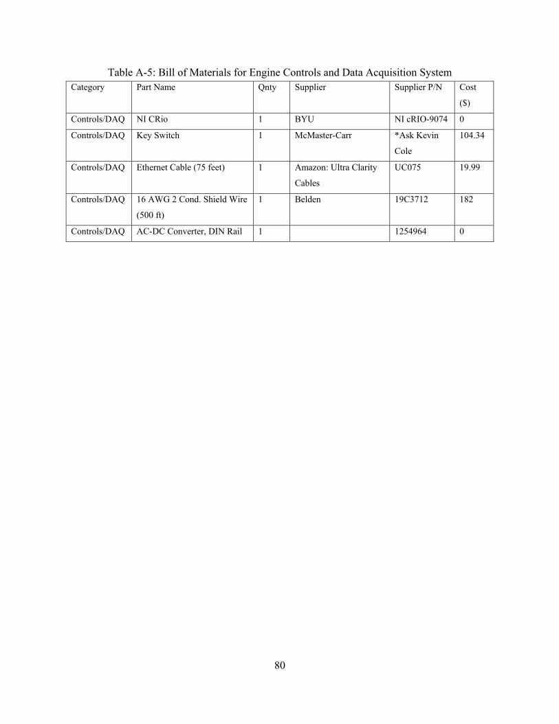
80
Table A-5: Bill of Materials for Engine Controls and Data Acquisition System Category Part Name Qnty Supplier Supplier P/N Cost
($)
Controls/DAQ NI CRio 1 BYU NI cRIO-9074 0
Controls/DAQ Key Switch 1 McMaster-Carr *Ask Kevin
Cole
104.34
Controls/DAQ Ethernet Cable (75 feet) 1 Amazon: Ultra Clarity
Cables
UC075 19.99
Controls/DAQ 16 AWG 2 Cond. Shield Wire
(500 ft)
1 Belden 19C3712 182
Controls/DAQ AC-DC Converter, DIN Rail 1
1254964 0
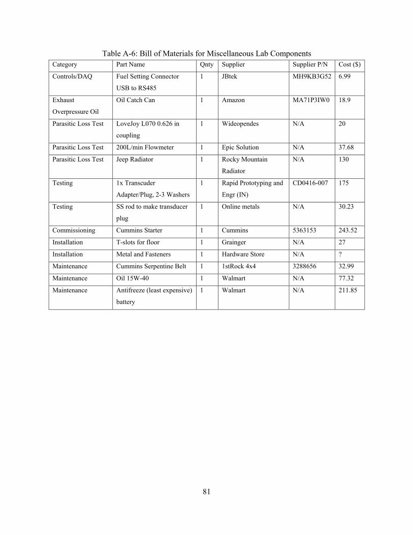
81
Table A-6: Bill of Materials for Miscellaneous Lab Components Category Part Name Qnty Supplier Supplier P/N Cost ($)
Controls/DAQ Fuel Setting Connector
USB to RS485
1 JBtek MH9KB3G52 6.99
Exhaust
Overpressure Oil
Oil Catch Can 1 Amazon MA71P3IW0 18.9
Parasitic Loss Test LoveJoy L070 0.626 in
coupling
1 Wideopendes N/A 20
Parasitic Loss Test 200L/min Flowmeter 1 Epic Solution N/A 37.68
Parasitic Loss Test Jeep Radiator 1 Rocky Mountain
Radiator
N/A 130
Testing 1x Transcuder
Adapter/Plug, 2-3 Washers
1 Rapid Prototyping and
Engr (IN)
CD0416-007 175
Testing SS rod to make transducer
plug
1 Online metals N/A 30.23
Commissioning Cummins Starter 1 Cummins 5363153 243.52
Installation T-slots for floor 1 Grainger N/A 27
Installation Metal and Fasteners 1 Hardware Store N/A ?
Maintenance Cummins Serpentine Belt 1 1stRock 4x4 3288656 32.99
Maintenance Oil 15W-40 1 Walmart N/A 77.32
Maintenance Antifreeze (least expensive)
battery
1 Walmart N/A 211.85
82
APPENDIX B. COUPLING ASSEMBLY DRAWINGS
This appendix outlines the coupling components purchased or designed.
• The flexible coupling and flange to shaft adapter were both purchased and supplier
documents are included.
• The flywheel was modified to enable connection to the flexible element; a drawing
outlining these modifications is included.
• Drawings for designed components (2.5-inch shaft, motor mounts, and driveline guard) are
included.
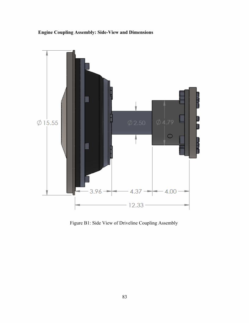
83
Figure B1: Side View of Driveline Coupling Assembly
Engine Coupling Assembly: Side-View and Dimensions
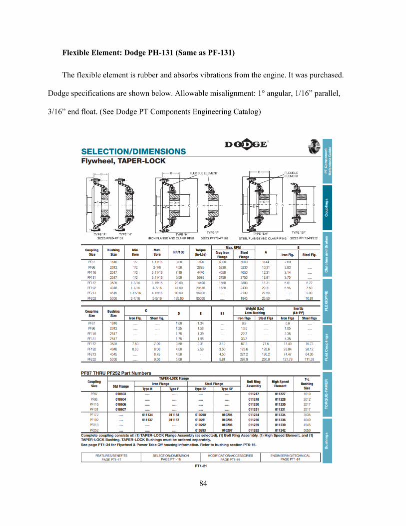
84
Flexible Element: Dodge PH-131 (Same as PF-131)
The flexible element is rubber and absorbs vibrations from the engine. It was purchased.
Dodge specifications are shown below. Allowable misalignment: 1° angular, 1/16” parallel,
3/16” end float. (See Dodge PT Components Engineering Catalog)
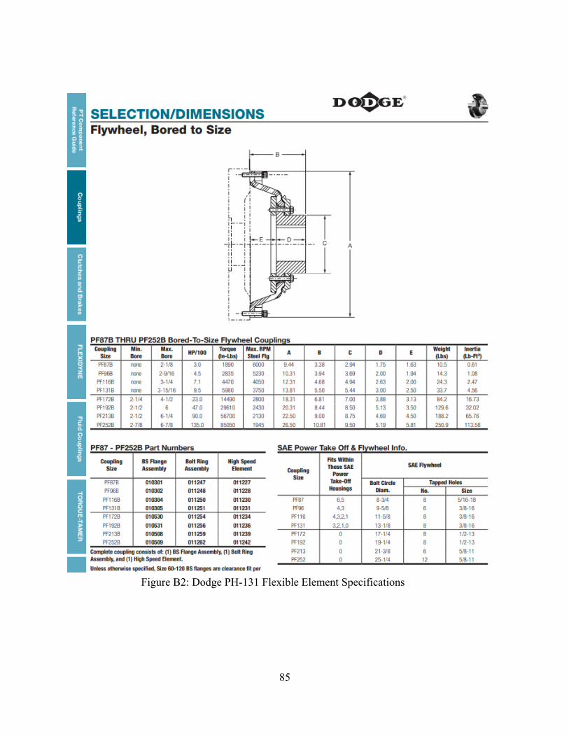
85
Figure B2: Dodge PH-131 Flexible Element Specifications
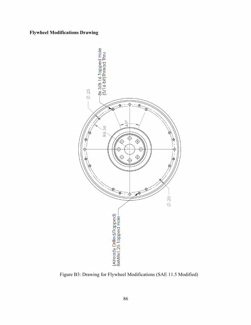
86
Figure B3: Drawing for Flywheel Modifications (SAE 11.5 Modified)
Flywheel Modifications Drawing
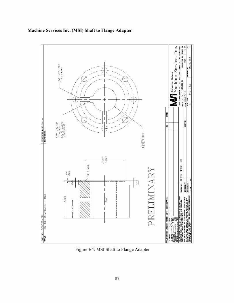
87
Figure B4: MSI Shaft to Flange Adapter
Machine Services Inc. (MSI) Shaft to Flange Adapter
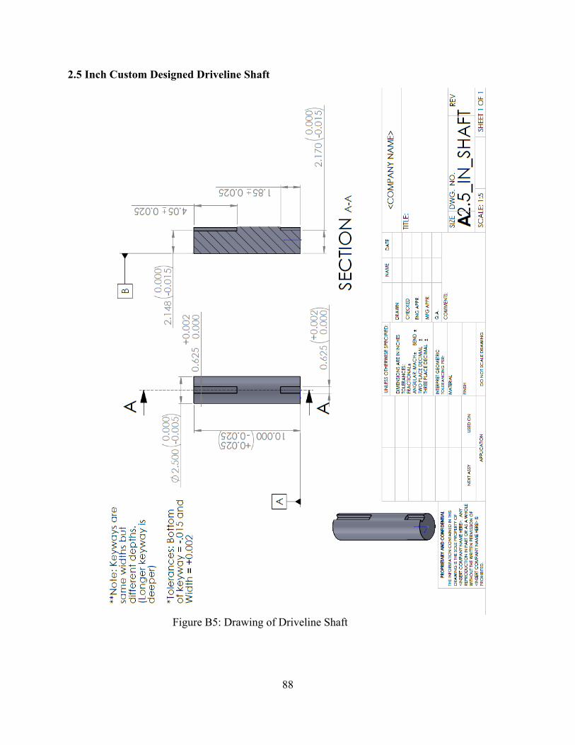
88
Figure B5: Drawing of Driveline Shaft
2.5 Inch Custom Designed Driveline Shaft
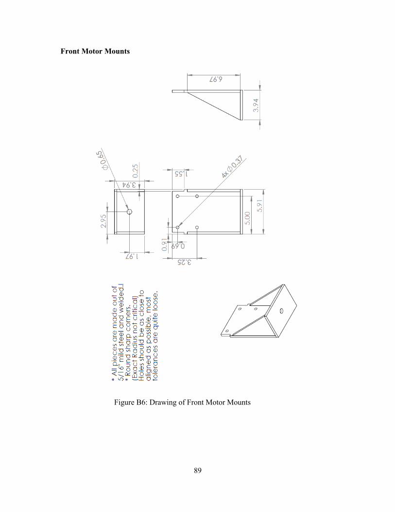
89
Figure B6: Drawing of Front Motor Mounts
Front Motor Mounts
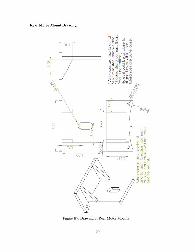
90
Figure B7: Drawing of Rear Motor Mounts
Rear Motor Mount Drawing
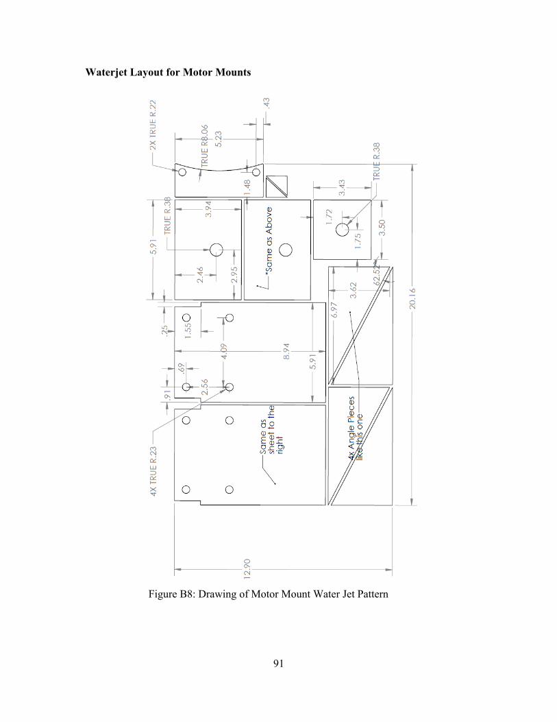
91
Figure B8: Drawing of Motor Mount Water Jet Pattern
Waterjet Layout for Motor Mounts
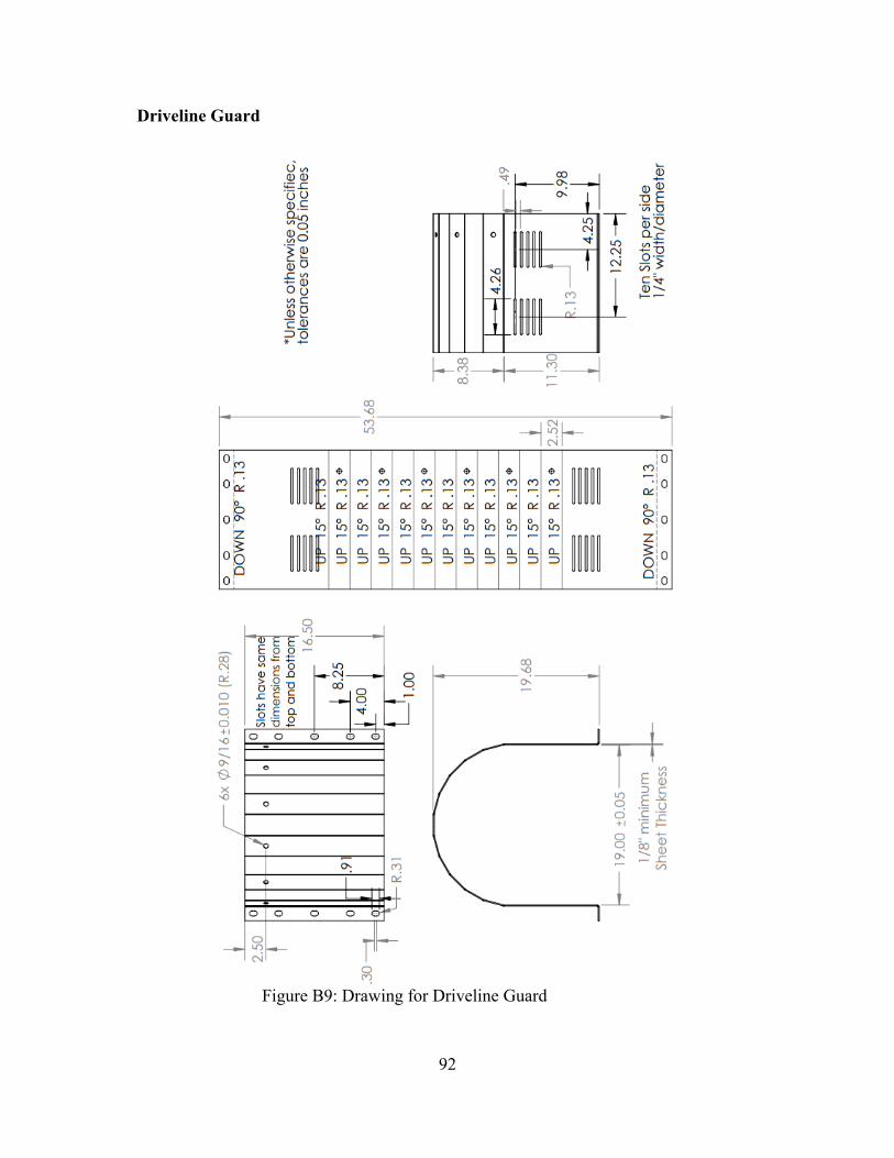
92
Figure B9: Drawing for Driveline Guard
Driveline Guard
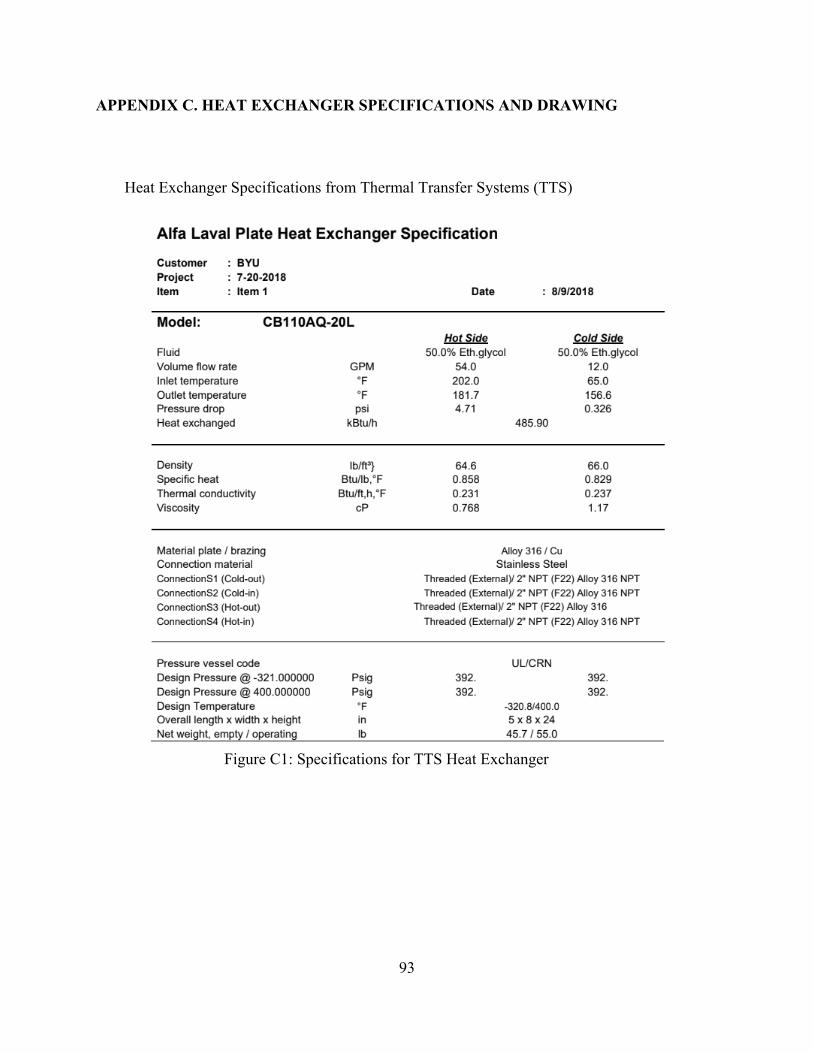
93
Figure C1: Specifications for TTS Heat Exchanger
APPENDIX C. HEAT EXCHANGER SPECIFICATIONS AND DRAWING
Heat Exchanger Specifications from Thermal Transfer Systems (TTS)
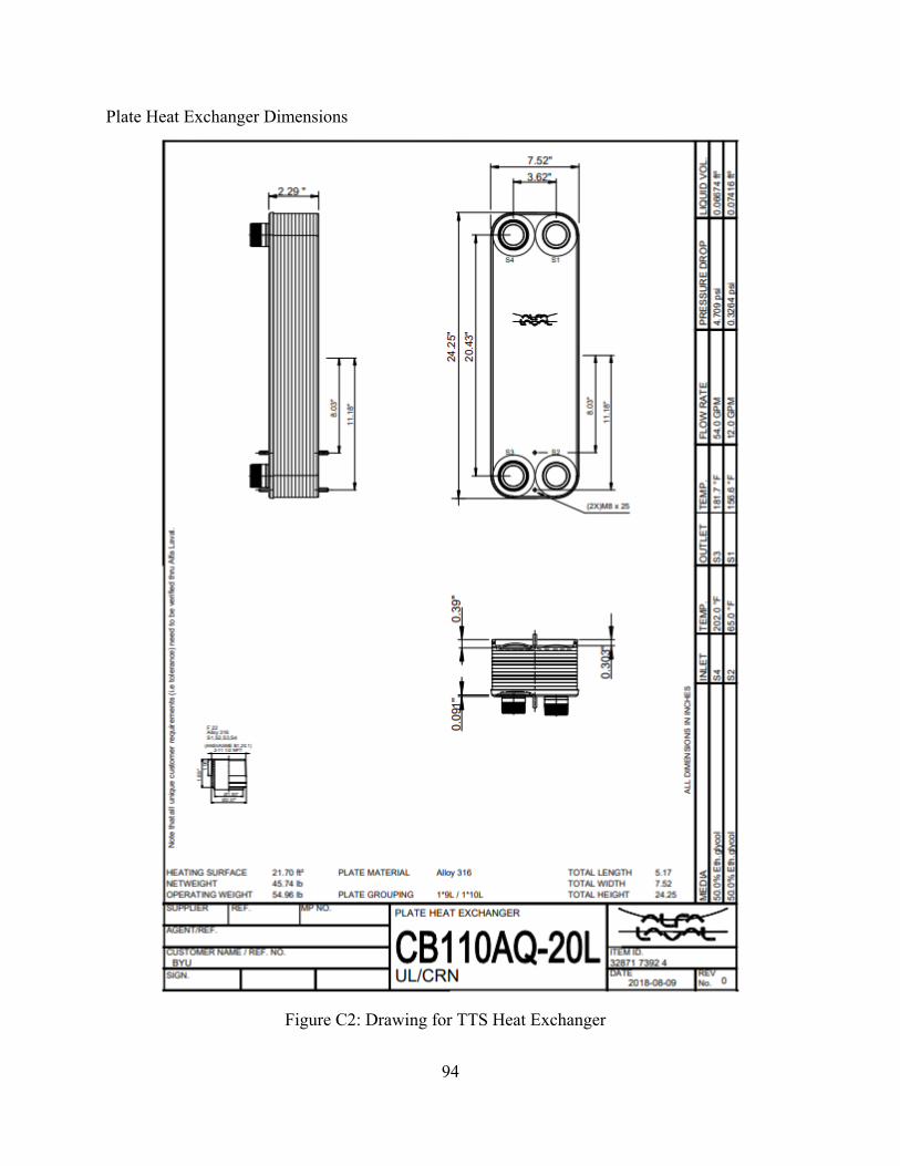
94
Figure C2: Drawing for TTS Heat Exchanger
Plate Heat Exchanger Dimensions
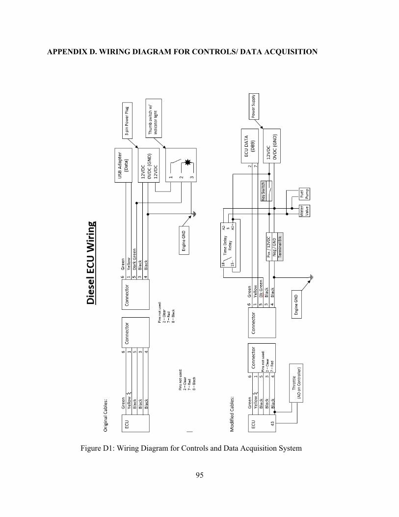
95
Figure D1: Wiring Diagram for Controls and Data Acquisition System
APPENDIX D. WIRING DIAGRAM FOR CONTROLS/ DATA ACQUISITION
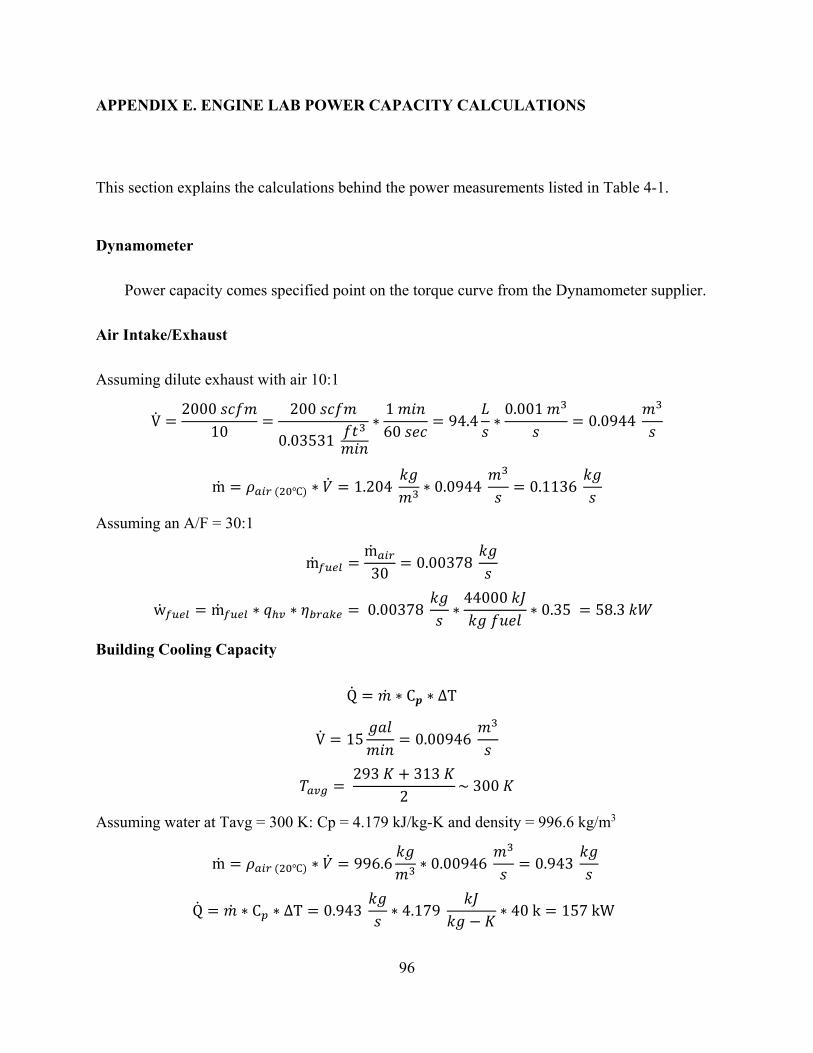
96
APPENDIX E. ENGINE LAB POWER CAPACITY CALCULATIONS
This section explains the calculations behind the power measurements listed in Table 4-1.
Dynamometer
Power capacity comes specified point on the torque curve from the Dynamometer supplier.
Air Intake/Exhaust
Assuming dilute exhaust with air 10:1
V =2000 𝑠𝑠𝑠𝑠𝑓𝑓𝑚𝑚
10=
200 𝑠𝑠𝑠𝑠𝑓𝑓𝑚𝑚
0.03531 𝑓𝑓𝑓𝑓3
𝑚𝑚𝐸𝐸𝐸𝐸
∗1 𝑚𝑚𝐸𝐸𝐸𝐸60 𝑠𝑠𝐸𝐸𝑠𝑠
= 94.4𝐿𝐿𝑠𝑠∗
0.001 𝑚𝑚3
𝑠𝑠= 0.0944
𝑚𝑚3
𝑠𝑠
m = 𝜌𝜌𝑎𝑎𝑤𝑤𝑟𝑟 (20℃) ∗ ��𝑉 = 1.204 𝑘𝑘𝐸𝐸𝑚𝑚3 ∗ 0.0944
𝑚𝑚3
𝑠𝑠= 0.1136
𝑘𝑘𝐸𝐸𝑠𝑠
Assuming an A/F = 30:1
m𝑓𝑓𝑜𝑜𝑟𝑟𝑟𝑟 =m𝑎𝑎𝑤𝑤𝑟𝑟
30= 0.00378
𝑘𝑘𝐸𝐸𝑠𝑠
w𝑓𝑓𝑜𝑜𝑟𝑟𝑟𝑟 = m𝑓𝑓𝑜𝑜𝑟𝑟𝑟𝑟 ∗ 𝑞𝑞ℎ𝑣𝑣 ∗ 𝜂𝜂𝑎𝑎𝑟𝑟𝑎𝑎𝐼𝐼𝑟𝑟 = 0.00378 𝑘𝑘𝐸𝐸𝑠𝑠∗
44000 𝑘𝑘𝑘𝑘𝑘𝑘𝐸𝐸 𝑓𝑓𝑓𝑓𝐸𝐸𝑙𝑙
∗ 0.35 = 58.3 𝑘𝑘𝑊𝑊
Building Cooling Capacity
Q = ��𝑚 ∗ C𝒑𝒑 ∗ ΔT
V = 15𝐸𝐸𝑇𝑇𝑙𝑙𝑚𝑚𝐸𝐸𝐸𝐸
= 0.00946 𝑚𝑚3
𝑠𝑠
𝑇𝑇𝑎𝑎𝑣𝑣𝑒𝑒 = 293 𝐾𝐾 + 313 𝐾𝐾
2~ 300 𝐾𝐾
Assuming water at Tavg = 300 K: Cp = 4.179 kJ/kg-K and density = 996.6 kg/m3
m = 𝜌𝜌𝑎𝑎𝑤𝑤𝑟𝑟 (20℃) ∗ ��𝑉 = 996.6𝑘𝑘𝐸𝐸𝑚𝑚3 ∗ 0.00946
𝑚𝑚3
𝑠𝑠= 0.943
𝑘𝑘𝐸𝐸𝑠𝑠
Q = ��𝑚 ∗ C𝑝𝑝 ∗ ΔT = 0.943 𝑘𝑘𝐸𝐸𝑠𝑠∗ 4.179
𝑘𝑘𝑘𝑘𝑘𝑘𝐸𝐸 − 𝐾𝐾
∗ 40 k = 157 kW
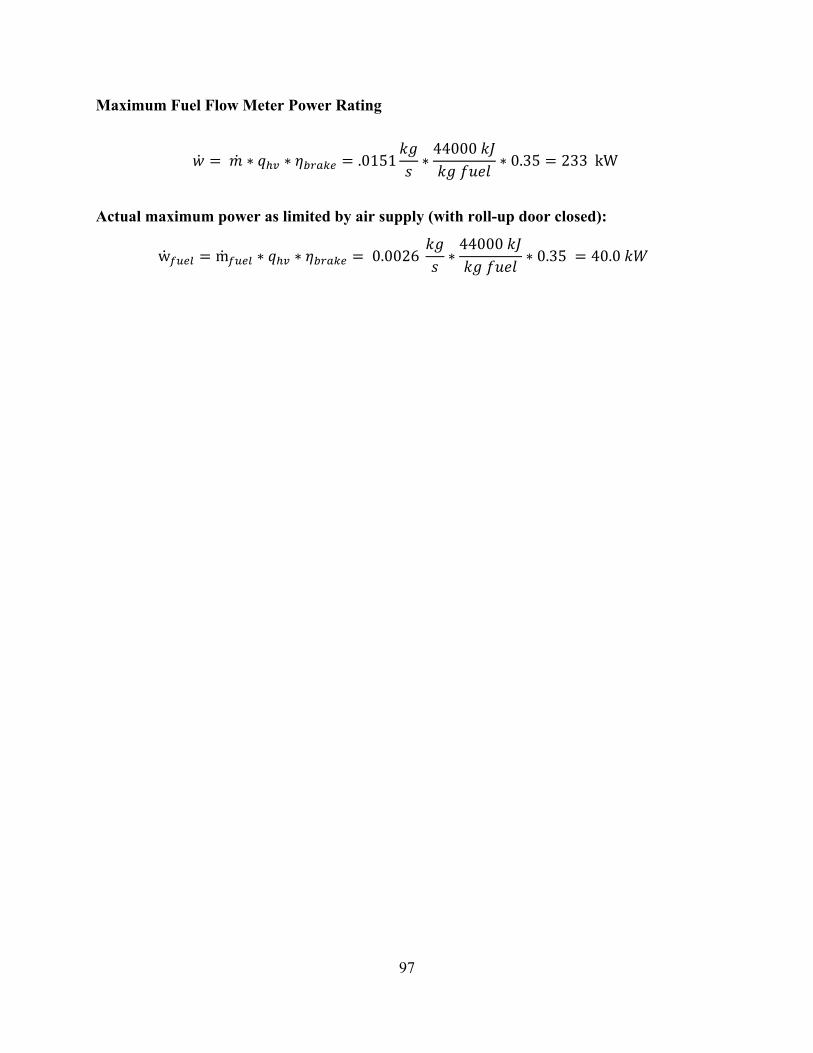
97
Maximum Fuel Flow Meter Power Rating
��𝑃 = ��𝑚 ∗ 𝑞𝑞ℎ𝑣𝑣 ∗ 𝜂𝜂𝑎𝑎𝑟𝑟𝑎𝑎𝐼𝐼𝑟𝑟 = .0151𝑘𝑘𝐸𝐸𝑠𝑠∗
44000 𝑘𝑘𝑘𝑘𝑘𝑘𝐸𝐸 𝑓𝑓𝑓𝑓𝐸𝐸𝑙𝑙
∗ 0.35 = 233 kW
Actual maximum power as limited by air supply (with roll-up door closed):
w𝑓𝑓𝑜𝑜𝑟𝑟𝑟𝑟 = m𝑓𝑓𝑜𝑜𝑟𝑟𝑟𝑟 ∗ 𝑞𝑞ℎ𝑣𝑣 ∗ 𝜂𝜂𝑎𝑎𝑟𝑟𝑎𝑎𝐼𝐼𝑟𝑟 = 0.0026 𝑘𝑘𝐸𝐸𝑠𝑠∗
44000 𝑘𝑘𝑘𝑘𝑘𝑘𝐸𝐸 𝑓𝑓𝑓𝑓𝐸𝐸𝑙𝑙
∗ 0.35 = 40.0 𝑘𝑘𝑊𝑊
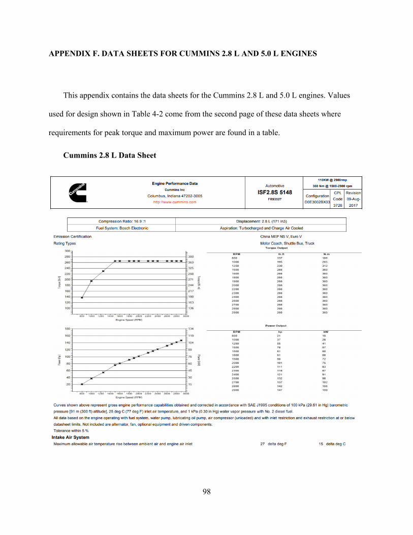
98
APPENDIX F. DATA SHEETS FOR CUMMINS 2.8 L AND 5.0 L ENGINES
This appendix contains the data sheets for the Cummins 2.8 L and 5.0 L engines. Values
used for design shown in Table 4-2 come from the second page of these data sheets where
requirements for peak torque and maximum power are found in a table.
Cummins 2.8 L Data Sheet
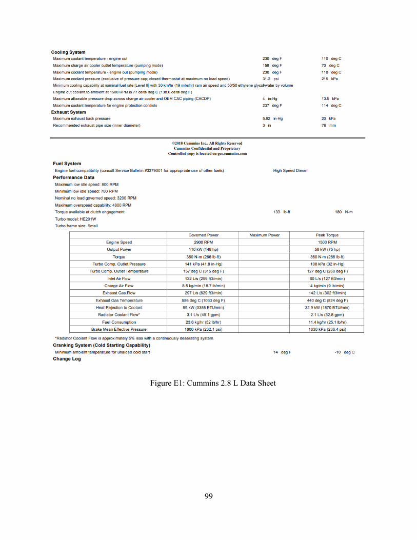
99
Figure E1: Cummins 2.8 L Data Sheet
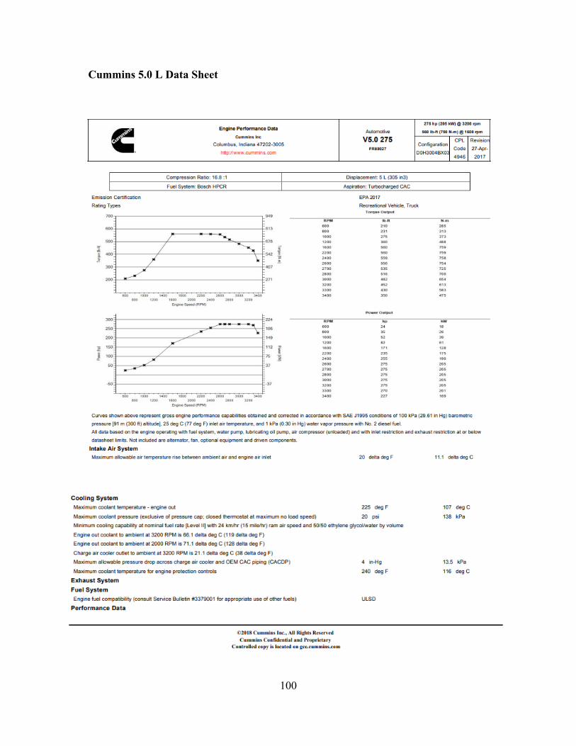
100
Cummins 5.0 L Data Sheet
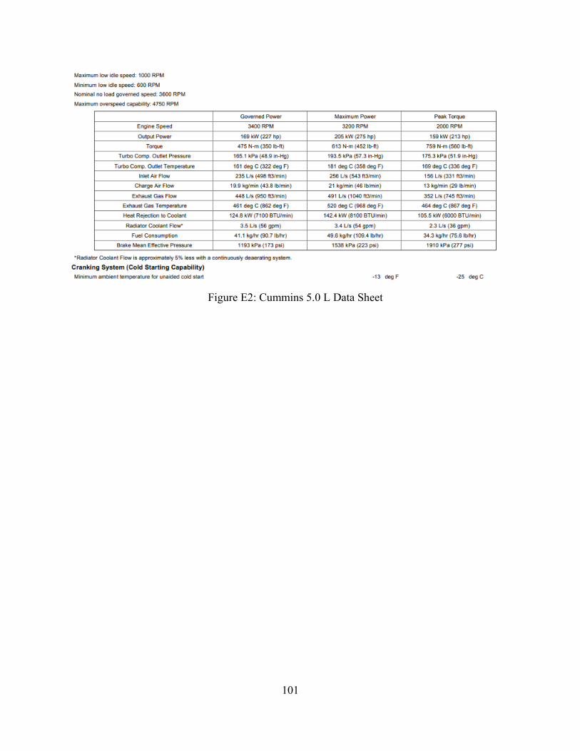
101
Figure E2: Cummins 5.0 L Data Sheet
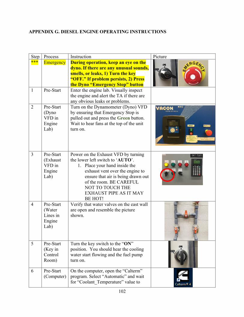
102
APPENDIX G. DIESEL ENGINE OPERATING INSTRUCTIONS
Step Process Instruction Picture *** Emergency During operation, keep an eye on the
dyno. If there are any unusual sounds, smells, or leaks, 1) Turn the key “OFF.” If problem persists, 2) Press the Dyno “Emergency Stop” button
1 Pre-Start Enter the engine lab. Visually inspect the engine and alert the TA if there are any obvious leaks or problems.
2 Pre-Start (Dyno VFD in Engine Lab)
Turn on the Dynamometer (Dyno) VFD by ensuring that Emergency Stop is pulled out and press the Green button. Wait to hear fans at the top of the unit turn on.
3 Pre-Start
(Exhaust VFD in Engine Lab)
Power on the Exhaust VFD by turning the lower left switch to ‘AUTO’.
1. Place your hand inside the exhaust vent over the engine to ensure that air is being drawn out of the room. BE CAREFUL NOT TO TOUCH THE EXHAUST PIPE AS IT MAY BE HOT!
4 Pre-Start (Water Lines in Engine Lab)
Verify that water valves on the east wall are open and resemble the picture shown.
5 Pre-Start (Key in Control Room)
Turn the key switch to the “ON” position. You should hear the cooling water start flowing and the fuel pump turn on.
6 Pre-Start
(Computer) On the computer, open the “Calterm” program. Select “Automatic” and wait for “Coolant_Temperature” value to
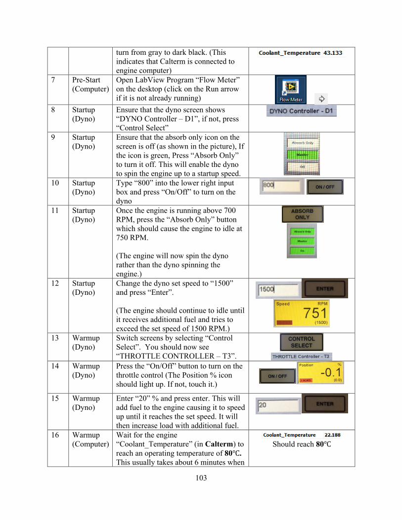
103
turn from gray to dark black. (This indicates that Calterm is connected to engine computer)
7 Pre-Start (Computer)
Open LabView Program “Flow Meter” on the desktop (click on the Run arrow if it is not already running)
8 Startup (Dyno)
Ensure that the dyno screen shows “DYNO Controller – D1”, if not, press “Control Select”
9
Startup (Dyno)
Ensure that the absorb only icon on the screen is off (as shown in the picture), If the icon is green, Press “Absorb Only” to turn it off. This will enable the dyno to spin the engine up to a startup speed.
10 Startup (Dyno)
Type “800” into the lower right input box and press “On/Off” to turn on the dyno
11 Startup (Dyno)
Once the engine is running above 700 RPM, press the “Absorb Only” button which should cause the engine to idle at 750 RPM. (The engine will now spin the dyno rather than the dyno spinning the engine.)
12 Startup (Dyno)
Change the dyno set speed to “1500” and press “Enter”. (The engine should continue to idle until it receives additional fuel and tries to exceed the set speed of 1500 RPM.)
13 Warmup (Dyno)
Switch screens by selecting “Control Select”. You should now see “THROTTLE CONTROLLER – T3”.
14 Warmup (Dyno)
Press the “On/Off” button to turn on the throttle control (The Position % icon should light up. If not, touch it.)
15 Warmup
(Dyno) Enter “20” % and press enter. This will add fuel to the engine causing it to speed up until it reaches the set speed. It will then increase load with additional fuel.
16 Warmup (Computer)
Wait for the engine “Coolant_Temperature” (in Calterm) to reach an operating temperature of 80℃. This usually takes about 6 minutes when
Should reach 80℃
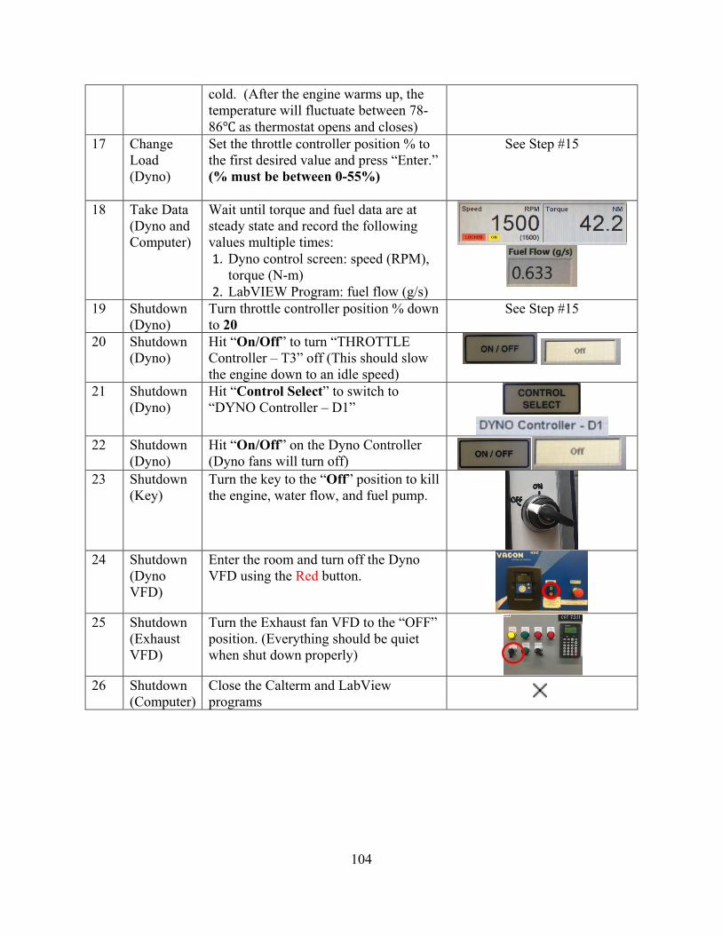
104
cold. (After the engine warms up, the temperature will fluctuate between 78-86℃ as thermostat opens and closes)
17 Change Load (Dyno)
Set the throttle controller position % to the first desired value and press “Enter.” (% must be between 0-55%)
See Step #15
18 Take Data (Dyno and Computer)
Wait until torque and fuel data are at steady state and record the following values multiple times: 1. Dyno control screen: speed (RPM),
torque (N-m) 2. LabVIEW Program: fuel flow (g/s)
19 Shutdown (Dyno)
Turn throttle controller position % down to 20
See Step #15
20 Shutdown (Dyno)
Hit “On/Off” to turn “THROTTLE Controller – T3” off (This should slow the engine down to an idle speed)
21 Shutdown (Dyno)
Hit “Control Select” to switch to “DYNO Controller – D1”
22 Shutdown
(Dyno) Hit “On/Off” on the Dyno Controller (Dyno fans will turn off)
23 Shutdown (Key)
Turn the key to the “Off” position to kill the engine, water flow, and fuel pump.
24 Shutdown
(Dyno VFD)
Enter the room and turn off the Dyno VFD using the Red button.
25 Shutdown
(Exhaust VFD)
Turn the Exhaust fan VFD to the “OFF” position. (Everything should be quiet when shut down properly)
26 Shutdown
(Computer) Close the Calterm and LabView programs
105
APPENDIX H. DIESEL ENGINE LABORATORY EXPERIMENT INSTRUCTIONS AND SAMPLE DATA
Key for - Diesel Lab 1: Diesel Brake Work, Power, and Efficiency
Assignment
1. Run the lab to take data for Torque and Fuel Flow Rate 2. Calculate the Brake Power (kW) and Fuel Power Efuel (kW) per cycle for each operating
condition. 3. Plot torque as a function of fuel flow rate with a single point as the average and error bars
showing one standard deviation for the four data points you collected (may not be able to see it if data has a small spread and values are large)
4. Plot the brake fuel conversion efficiency as a function of fuel flow rate (load) showing a single data point for the average and error bars representing plus or minus one standard deviation of the data collected.
5. Discuss why the brake fuel conversion efficiency increases with increasing load?
106
Answers
The Answers should resemble, the following data, though the lab data will not include the 60 and 70% Pedal Positions. Data (Taken on 9/27/19)
1. Run the lab to take data for Torque and Fuel Flow Rate 2. Calculate the Brake Power (kW) and Fuel Power Efuel (kW) per cycle for each operating
condition.
Power Data Calculated Values
RPM % Throttle Torque (N-m)
m_dot (g/s) Power (kW)
Heating Power (kW) Efficiency
750 0 5 0.188 0.39269908 8.272 0.047473 0 6 0.2 0.4712389 8.8 0.05355 0 7 0.149 0.54977871 6.556 0.083859 0 10 0.159 0.78539816 6.996 0.112264 1500 15 51.2 0.717 8.04247719 31.548 0.254928 15 53.2 0.663 8.35663646 29.172 0.286461 15 52.2 0.686 8.19955683 30.184 0.271652 15 52.8 0.71 8.29380461 31.24 0.265487 1500 20 68 0.811 10.681415 35.684 0.299333 20 69.6 0.774 10.9327424 34.056 0.321023 20 67.2 0.809 10.5557513 35.596 0.296543 20 69.4 0.774 10.9013265 34.056 0.3201 1500 30 113 1.195 17.7499985 52.58 0.337581 30 111.7 1.12 17.545795 49.28 0.356043 30 112.6 1.171 17.6871666 51.524 0.34328 30 114.2 1.125 17.9384941 49.5 0.362394 1500 40 157.4 1.445 24.7243342 63.58 0.38887 40 156.7 1.528 24.6143784 67.232 0.366111 40 158 1.485 24.818582 65.34 0.379837 40 156 1.577 24.5044227 69.388 0.353151 1500 50 211 1.95 33.1438025 85.8 0.386291 50 209 2.001 32.8296432 88.044 0.372878 50 210 1.995 32.9867229 87.78 0.375789 50 211.8 2.033 33.2694662 89.452 0.371925 1500 55 227 2.18 35.6570766 95.92 0.371738 55 224.5 2.15 35.2643775 94.6 0.372774 55 226.5 2.17 35.5785368 95.48 0.372628 55 225 2.14 35.3429174 94.16 0.37535
107
3. Plot torque as a function of fuel flow rate with a single point as the average and error bars showing one standard deviation for the four data points you collected (may not be able to see it if data has a small spread and values are large)
4. Plot the brake fuel conversion efficiency as a function of fuel flow rate (load) showing a single data point for the average and error bars representing plus or minus one standard deviation of the data collected.
108
5. Discuss why the brake fuel conversion efficiency increases with increasing load?
𝜂𝜂𝑎𝑎 = ��𝑃𝑎𝑎
𝑞𝑞ℎ𝑣𝑣 ∗ 𝑚𝑚𝑓𝑓=��𝑃𝑤𝑤,𝑒𝑒 − ��𝑃𝑝𝑝 − ��𝑃𝑓𝑓
𝑞𝑞ℎ𝑣𝑣 ∗ 𝑚𝑚𝑓𝑓=
��𝑃𝑤𝑤,𝑒𝑒𝑞𝑞ℎ𝑣𝑣 ∗ 𝑚𝑚𝑓𝑓
−��𝑃𝑝𝑝
𝑞𝑞ℎ𝑣𝑣 ∗ 𝑚𝑚𝑓𝑓−
��𝑃𝑓𝑓𝑞𝑞ℎ𝑣𝑣 ∗ 𝑚𝑚𝑓𝑓
Of the Terms on the right side, the left term is nearly constant as both the numerator and denominator increase. The middle term is nearly 0 for a diesel engine with no pumping work (or that term even becomes a slight positive for turbocharged engine. The right term decreases or the friction becomes a smaller portion due to the fact that the friction remains nearly constant for a constant engine speed and the denominator keeps increasing with increasing fuel flow.
Additional Plots for Reference
109
Key for - Diesel Lab 2: Diesel Emissions, Brake Work, and Efficiency
Assignment
1. Run the lab to take data for Torque, Fuel Flow Rate, NOx, CO, CO2, O2. 2. Plot the emissions concentrations as a function of fuel flow with error bars. (Plot both
PPM and Vol % on the same chart. Plot PPM (NOx, SO2, CO) on the left axis and Vol% (CO2 and O2) on the right axis and differentiate each with a legend. If printing in black and white, change the points to stars, boxes, … to clearly differentiate the concentrations.)
3. Discuss trends in emissions verses fuel flow rate (load). Some observations should include:
a. The scale of NO and CO compared to O2, CO2? b. The relationship between CO2 and O2 with change in fuel flow? c. How does NOx change with fuel flow? d. How does O2 change with fuel flow? e. How does CO2 change with fuel flow? f. How does CO change with change in fuel flow?
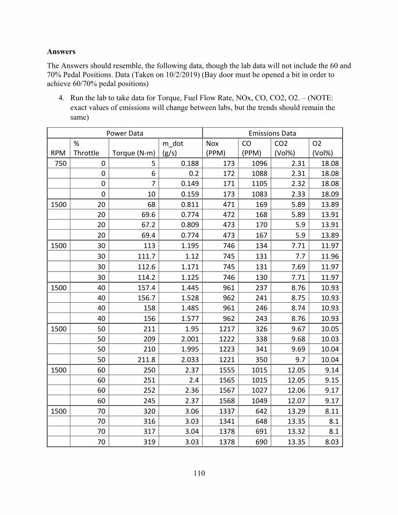
110
Answers
The Answers should resemble, the following data, though the lab data will not include the 60 and 70% Pedal Positions. Data (Taken on 10/2/2019) (Bay door must be opened a bit in order to achieve 60/70% pedal positions)
4. Run the lab to take data for Torque, Fuel Flow Rate, NOx, CO, CO2, O2. – (NOTE: exact values of emissions will change between labs, but the trends should remain the same)
Power Data Emissions Data
RPM % Throttle Torque (N-m)
m_dot (g/s)
Nox (PPM)
CO (PPM)
CO2 (Vol%)
O2 (Vol%)
750 0 5 0.188 173 1096 2.31 18.08 0 6 0.2 172 1088 2.31 18.08 0 7 0.149 171 1105 2.32 18.08 0 10 0.159 173 1083 2.33 18.09 1500 20 68 0.811 471 169 5.89 13.89 20 69.6 0.774 472 168 5.89 13.91 20 67.2 0.809 473 170 5.9 13.91 20 69.4 0.774 473 167 5.9 13.89 1500 30 113 1.195 746 134 7.71 11.97 30 111.7 1.12 745 131 7.7 11.96 30 112.6 1.171 745 131 7.69 11.97 30 114.2 1.125 746 130 7.71 11.97 1500 40 157.4 1.445 961 237 8.76 10.93 40 156.7 1.528 962 241 8.75 10.93 40 158 1.485 961 246 8.74 10.93 40 156 1.577 962 243 8.76 10.93 1500 50 211 1.95 1217 326 9.67 10.05 50 209 2.001 1222 338 9.68 10.03 50 210 1.995 1223 341 9.69 10.04 50 211.8 2.033 1221 350 9.7 10.04 1500 60 250 2.37 1555 1015 12.05 9.14 60 251 2.4 1565 1015 12.05 9.15 60 252 2.36 1567 1027 12.06 9.17 60 245 2.37 1568 1049 12.07 9.17 1500 70 320 3.06 1337 642 13.29 8.11 70 316 3.03 1341 648 13.35 8.1 70 317 3.04 1378 691 13.32 8.1 70 319 3.03 1378 690 13.35 8.03
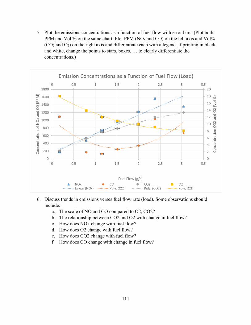
111
5. Plot the emissions concentrations as a function of fuel flow with error bars. (Plot both PPM and Vol % on the same chart. Plot PPM (NOx and CO) on the left axis and Vol% (CO2 and O2) on the right axis and differentiate each with a legend. If printing in black and white, change the points to stars, boxes, … to clearly differentiate the concentrations.)
6. Discuss trends in emissions verses fuel flow rate (load). Some observations should
include: a. The scale of NO and CO compared to O2, CO2? b. The relationship between CO2 and O2 with change in fuel flow? c. How does NOx change with fuel flow? d. How does O2 change with fuel flow? e. How does CO2 change with fuel flow? f. How does CO change with change in fuel flow?
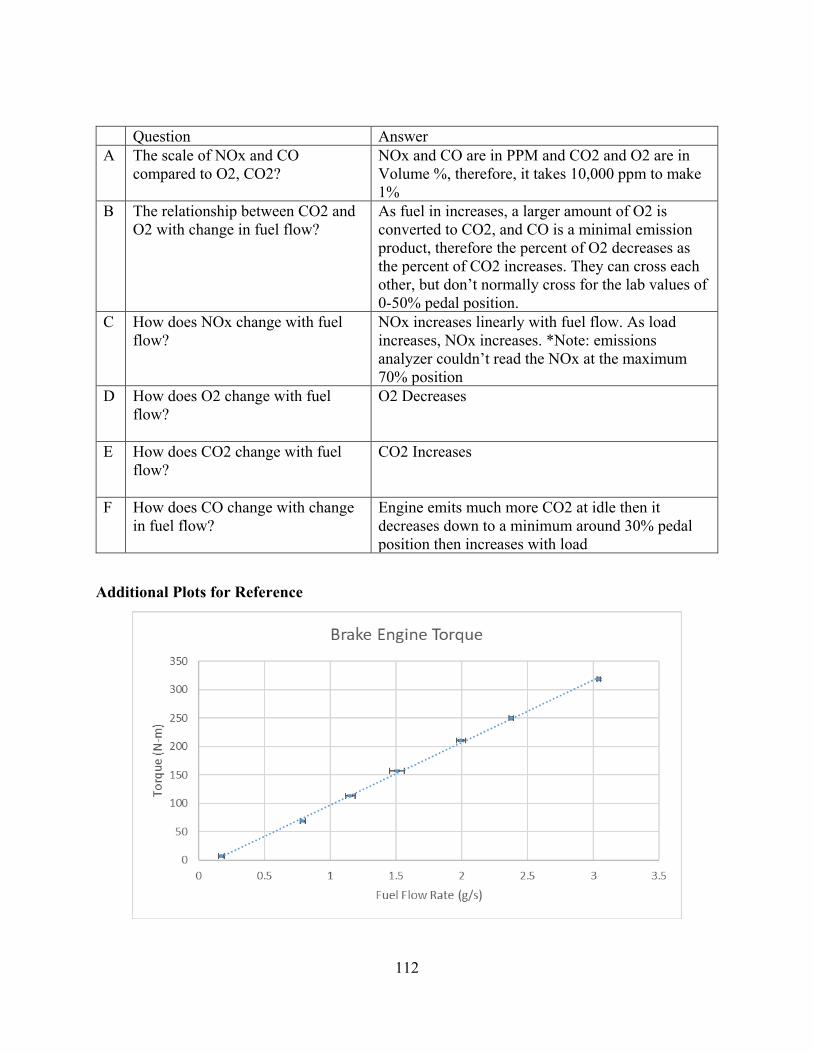
112
Question Answer A The scale of NOx and CO
compared to O2, CO2? NOx and CO are in PPM and CO2 and O2 are in Volume %, therefore, it takes 10,000 ppm to make 1%
B The relationship between CO2 and O2 with change in fuel flow?
As fuel in increases, a larger amount of O2 is converted to CO2, and CO is a minimal emission product, therefore the percent of O2 decreases as the percent of CO2 increases. They can cross each other, but don’t normally cross for the lab values of 0-50% pedal position.
C How does NOx change with fuel flow?
NOx increases linearly with fuel flow. As load increases, NOx increases. *Note: emissions analyzer couldn’t read the NOx at the maximum 70% position
D How does O2 change with fuel flow?
O2 Decreases
E How does CO2 change with fuel flow?
CO2 Increases
F How does CO change with change in fuel flow?
Engine emits much more CO2 at idle then it decreases down to a minimum around 30% pedal position then increases with load
Additional Plots for Reference
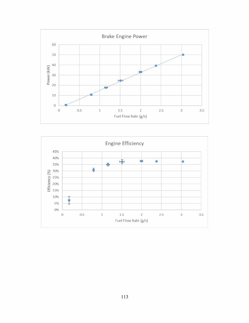
113