Accepted by Biomaterials on 09/27/01, In press, 2002

Constitutive Modeling of Ultra-High Molecular Weight Polyethylene Under Large-Deformation and Cyclic Loading

Conditions

J.S. Bergström*1, S.M. Kurtz1, C.M. Rimnac2, A.A. Edidin3

1Exponent, Inc., 21 Strathmore Rd, Natick, MA

2Orthopaedic Implant Retrieval Analysis Laboratory, Departments of Orthopaedics and Mechanical and Aerospace Engineering, Case Western Reserve University, Cleveland, OH

3Howmedica Osteonics Corp., 59 Route 17, Allendale, NJ

*Corresponding Author:

Jörgen S. Bergström Exponent, Inc. 21 Strathmore Rd. Natick, MA 01760 Tel: 508-652-8500 Fax: 508-647-1899 Email: jbergstrom@exponent.com

Submitted: May, 2001

New Contact Email: Jorgen@PolymerFEM.com

3

Abstract

When subjected to a monotonically increasing deformation state, the mechanical behavior of

UHMWPE is characterized by a linear elastic response followed by distributed yielding and strain

hardening at large deformations. During the unloading phases of an applied cyclic deformation process,

the response is characterized by nonlinear recovery driven by the release of stored internal energy. A

number of different constitutive theories can be used to model these experimentally observed events.

We compare the ability of the J2-plasticity theory, the “Arruda-Boyce” model, the “Hasan-Boyce”

model, and the “Bergström-Boyce” model to reproduce the observed mechanical behavior of

UHMWPE. In addition a new hybrid model is proposed, which incorporates many features of the

previous theories. This hybrid model is shown to most effectively predict the experimentally observed

mechanical behavior of UHMWPE.

Key Words: constitutive modeling, UHMWPE, time-dependence, cyclic loading

4

Introduction

For more than 35 years ultra-high molecular weight polyethylene (UHMWPE) has been used

successfully as a bearing material in total joint replacement components [1]. As an example, in 1998

approximately 1.4 million patients worldwide underwent total joint replacement surgery for treatment of

degenerative joint disease [2]. It has been recognized that wear damage to UHMWPE total joint

components is a significant clinical problem limiting the lifetime of joint arthroplasties. Long-term

complications in total joint replacement, such as loosening and infection, have been correlated to the

foreign body reaction to the UHMWPE debris found in the surrounding tissues and produced from

wear damage to the articulating surfaces [3-5]. Although the wear mechanisms appear to be different in

knee and hip components, the plastic flow behavior of UHMWPE [6-10] has been related to the

clinical performance in both types of joint replacement components.

The true stress strain relationship provides useful information about the yielding and plastic flow

behavior of polymers [11-26]. Therefore, in this work the description of the stress-strain response is

expressed in terms of true stress and true strain, where for uniaxial loading true stress is defined as

applied force divided by current area (this stress measure is also referred to as Cauchy stress) and true

strain is defined by the logarithm of the current specimen length divided by the original specimen length

(also referred to as Hencky strain). A detailed understanding of the yielding and plastic flow behavior,

particularly under multiaxial loading conditions, is needed to further develop micromechanical wear and

fracture models of UHMWPE [6,8].

A number of different finite element models have been developed that predict the multiaxial

stress state at the articulating surface and beneath the center of contact in UHMWPE acetabular, tibial,

and patellar components [27-33]. A necessary component in the development of the models is an

accurate prediction of the true stress-strain behavior. In the past this relation has been represented

using classical isotropic, rate independent plasticity using a Mises yield criterion to approximate the

nonlinear mechanical response of the polymer [34]. In classical plasticity theory, the total strain is

calculated as the sum of elastic and plastic strains, and the plastic deformation is assumed to be

5

incompressible. It has been experimentally observed that during elastic processes the Poisson’s ratio of

UHMWPE is about 0.46 [35]. The assumption that the plastic deformation of UHMWPE is

incompressible has also been verified [36].

A number of different finite element analyses of UHMWPE components from both hip and knee

replacements have been conducted to predict the effect of load, geometry and material properties on

the stress and strain distributions in these components [27,30,37-39]. Early models only incorporated

monotonic loading and were based on bilinear elastic or elastic-plastic approximations of the stress-

strain behavior of UHMWPE. These simulations of total joint replacements generally adopted a

deviatoric rate-independent plasticity approach with a Mises yield surface with an associated flow rule

followed by isotropic hardening (this model approach is referred to as classical J2 plasticity theory in the

following) to model UHMWPE [27,29-33,36,38]. For example, Estupiñan et al. [38] recently

simulated the effect of a moving cyclic load on the stress distributions near the surface of an idealized,

two dimensional UHMWPE block, intended to represent a generic tibial component of a total knee

replacement. The UHMWPE was modeled using a quadrilinear approximation of the yielding behavior

up to a true strain of 0.12, and was simulated by classical isotropic J2 plasticity theory [27]. The

researchers observed that cyclic stability (“shakedown”) occurred within five cycles of loading, and that

residual tensile stresses developed the articulating surface.

However, investigation of unloading behavior and studies of permanent plastic deformations in

UHMWPE has shown that classical plasticity theory greatly overpredicts the permanent strains upon

unloading [36]. Thus, using classical plasticity theory to simulate cyclic loading in UHMWPE implants

may lead to exaggerated predictions in residual strains and stresses [36].

An investigation of cyclic contact behavior of UHMWPE tibial knee components has also been

performed by Ishikawa et al. [39]. In their study, they modeled the UHMWPE using a constitutive

model for cyclic plasticity, but the parameters of the model were based on cyclic strain experiments with

a strain amplitude of only 2%. Ishikawa’s model further assumed that the stress-strain behavior of

UHMWPE reached cyclic stability or shakedown after three cycles of loading, regardless of the strain

amplitude.

6

Thus, previous studies highlight the need to establish and validate accurate constitutive theories

for UHMWPE in order to be able to better predict the stress and strain distributions in a component

undergoing in vivo cyclic loading. A family of physically-inspired constitutive theories have been

established which incorporate viscoplasticity, as well as viscoelasticity, based upon fundamental,

statistically-based deformation mechanisms in polymers [40-42]. These constitutive theories, which will

be referred to as “Arruda-Boyce” (“AB” [42]), “Hasan-Boyce” (“HB” [40]), and “Bergström-Boyce”

(“BB” [41]) models for viscoelastic/viscoplastic behavior in polymers, have thus far not been widely

applied to UHMWPE. In addition to these existing models, a newly developed constitutive framework

is also presented here. This new model will be referred to as the “hybrid model” (“HM”).

The goal of the present study was to evaluate the feasibility of the J2- plasticity, AB, BB, HB,

and HM constitutive theories for simulating the mechanical behavior of virgin UHMWPE under

monotonic and cyclic loading conditions. To compare these different constitutive theories, predictions

of five different experimental data sets (small, intermediate, and large monotonic deformation, cyclic

deformation, and the combined set of all experimental data) were computed. For each model and each

loading case the most appropriate material parameters were found and the quality of the predicted

response compared to the experimental behavior was quantified with the coefficient of determination, r2.

Constitutive Theories for Polymers

The mechanical behavior of glassy polymeric materials is time- and temperature-dependent, and

the stress-strain behavior even prior to yield is often nonlinear due to the distribution and evolution in

plastic shear strength with deformation. Thus, constitutive relationships for polymeric materials should

incorporate a continuous description of material response as it transitions from linear elastic to

viscoelastic/viscoplastic behavior.

A large number of different constitutive models for glassy polymers have been developed

throughout the years, significantly more than can be summarized in this paper. The approach taken here

is to compare some of the models that have recently been used in the literature to predict the behavior

of UHMWPE (J2-plasticity, and the BB model [41]), and also compare some promising models that

7

have not yet been applied to UHMWPE (AB, HB). In Appendix B, these different models are

described in detail using a unified and consistent nomenclature (following Gurtin [43] and Silhavý [44]),

enabling a direct comparison between the different model frameworks. Note that the presented models

are not necessarily identical to the original developments; a unified nomenclature is introduced and by

considering the particular behavior of UHMWPE it has been possible to simplify certain expressions.

In addition to the existing models, a newly developed model for UHMWPE has been

developed. This model is presented in the next section.

The Hybrid Model (HM)

It has been shown that the deformational resistance of the amorphous phase of a semi-

crystalline polymer, such as UHMWPE, is lower than the deformational resistance of the crystalline

phase [22]. Consequently, at small applied strains, the applied deformation will be localized into the

amorphous phase and the lamellar crystals will remain relatively undeformed. At larger strains the

microstructure changes from randomly oriented lamellae to a more oriented structure with alternating

crystalline and amorphous layers. The morphological changes that occur with applied deformation are

difficult to quantify for a semicrystalline polymer. Therefore, the approach taken here is to conceptually

homogenize the microstructure into one phase whose internal micromechanical state is tracked as a

function of applied deformation. The kinematic framework used for doing this is similar to the AB and

HB models in that the applied deformation gradient is decomposed into elastic and plastic components,

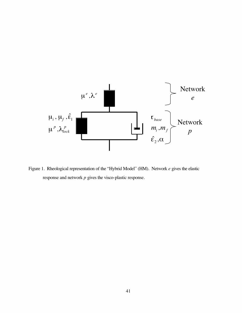
F = F eF p , see Figure 1. Hence, the Cauchy stress acting on the system can be obtained from the

linear elastic relationship presented in Equation (1):

( )1 2 tre e e eeJ

µ λ = + T E E 1 , (1)

where ln[ ]e e=E V is the logarithmic true strain, det[ ]e eJ = F , and µe ,λe are Lamé’s constants.

The influence of the lamellae in the crystalline phase, however, is not only to enhance the stress

and strain in the amorphous matrix but also to alter the amorphous phase in the vicinity of the crystals

[22] and to contribute energetically to the deformation resistance. The influence of this behavior can be

8

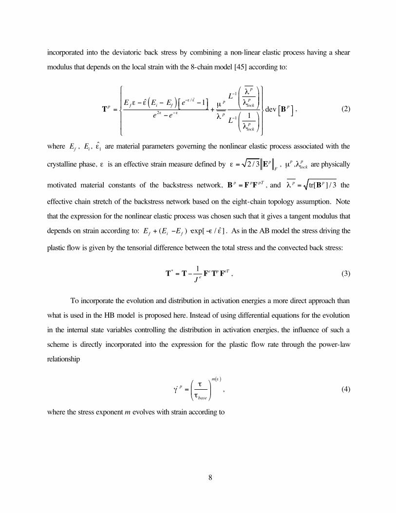
incorporated into the deviatoric back stress by combining a non-linear elastic process having a shear

modulus that depends on the local strain with the 8-chain model [45] according to:

( )

1ˆ/

21

ˆ 1dev

1

p

pplockf i fp p

p

plock

LE E E e

e eL

ε ε

ε ε

λλε ε µ

λλ

−

−

−−

− − − = + −

T B , (2)

where Ef , Ei , ˆ ε 1 are material parameters governing the nonlinear elastic process associated with the

crystalline phase, ε is an effective strain measure defined by 2 / 3 pF

ε = E , µp ,λlockp are physically

motivated material constants of the backstress network, p p pT=B F F , and tr[ ] / 3p pλ = B the

effective chain stretch of the backstress network based on the eight-chain topology assumption. Note

that the expression for the nonlinear elastic process was chosen such that it gives a tangent modulus that

depends on strain according to: ˆ( ) exp[ / ]f i fE E E ε ε+ − ⋅ − . As in the AB model the stress driving the

plastic flow is given by the tensorial difference between the total stress and the convected back stress:

* 1 e p eTeJ

= −T T F T F , (3)

To incorporate the evolution and distribution in activation energies a more direct approach than

what is used in the HB model is proposed here. Instead of using differential equations for the evolution

in the internal state variables controlling the distribution in activation energies, the influence of such a

scheme is directly incorporated into the expression for the plastic flow rate through the power-law

relationship

( )m

p

base

ετ

γτ

=

& , (4)

where the stress exponent m evolves with strain according to

9

( ) ( ) 22

ˆ1 , if ˆ

, otherwise

f i f

f

m m mm

m

αε

ε εε ε

+ − − < =

(5)

and mi , m f , 2ε̂ , α are material constants and ε has the same definition as before, i.e.

2 /3 | | ||pFε = E . This relationship gives very similar behavior as the Arrhenius-type exponential

representation that is used in the Arruda-Boyce model, with the additional benefit that the flow rate goes

to zero as the driving shear stress goes to zero. Here, for numerical efficiency and ease of finding the

necessary material coefficients, the power-law exponent m is taken to evolve with the local strain from

an initial value of mi in an undeformed local strain state to a value of m f at large local strains. The key

feature of Equation (5) is that it enables a distributed yielding process by implicitly incorporating the

evolution in the activation behavior.

Materials and Methods

The proposed constitutive theories were tested against previously collected stress-strain data in

monotonic tension, monotonic compression, and fully reversed cyclic tension-compression [36,46].

The previous data were collected at two institutions using bulk cylindrical specimens fabricated from

extruded rods of UHMWPE converted using the same resin grade (GUR 4150 HP, Ticona, Bayport,

TX). The experiments were all conducted at room temperature on unirradiated UHMWPE employing a

variety of strain rates and strain ranges, as summarized in Table 1.

The four data sets contained the results of “small strain,” “intermediate strain,” “large strain,” and

“cyclic strain” experiments (Table 1, [36,46]). The first three sets included data from monotonic loading

experiments, whereas the fourth set contained the results of one cycle of fully reversed, cyclic tension-

compression [46]. The “small strain” data set (collected in uniaxial compression) was of greatest

relevance for the strain ranges subjected to artificial hip components [30], whereas the “intermediate

strain” set (collected in uniaxial tension and compression) contained data of relevance to knee

components, which may be subjected to effective true strains of up to 0.12 [30]. The “intermediate

10

strain” set also contained data collected at two different strain rates (0.01 and 0.1 s-1). The “large strain”

set contained uniaxial tensile data to failure at a constant crosshead displacement rate (30 mm/s), and

was considered to be relevant for localized damage modes related to plastic deformation and wear

[36]. The four individual data sets outlined in Table 1 were therefore applicable to a wide range of

potential clinically relevant orthopaedic applications. Ideally, a suitable constitutive theory should predict

the mechanical behavior of UHMWPE for all of these experimental test conditions. Consequently, a fifth

combined data set was created, which contained all of the data for the “small strain,” “intermediate

strain,” “large strain,” and “cyclic strain” sets.

The constitutive theories presented in the previous section were implemented in Matlab

(Mathworks, Natick, MA). An initial set of material parameters was determined for each theory by

following the procedures outlined in the original papers [41,47]. For each model, an optimal set of

material parameters was then found from the initial set by using a numerical unconstrained nonlinear

optimization algorithm based on the Nelder-Mead simplex search method. The objective function used

to rank different sets of material parameters was defined as the sum of the squared differences between

the experimental and predicted data. The advantage of this objective function is that it gives the optimal

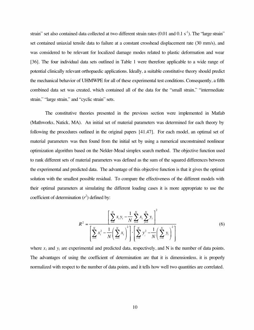
solution with the smallest possible residual. To compare the effectiveness of the different models with

their optimal parameters at simulating the different loading cases it is more appropriate to use the

coefficient of determination (r2) defined by:

2

1 1 122 2

2 2

1 1 1 1

1

1 1i

N N N

i i i ii i j

N N N N

i i ii i i i

x y x yN

R

x x y yN N

= = =

= = = =

−

= − ⋅ −

∑ ∑ ∑

∑ ∑ ∑ ∑ (6)

where xi and yi are experimental and predicted data, respectively, and N is the number of data points.

The advantages of using the coefficient of determination are that it is dimensionless, it is properly

normalized with respect to the number of data points, and it tells how well two quantities are correlated.

11

Results

The material parameters used in the J2-plasticity model are summarized in Table 3. In this table

the material parameters giving the best overall predictions of each data set are given. The predicted

behavior using the J2-plasticity model is piecewise linear, and for practical purposes the number of

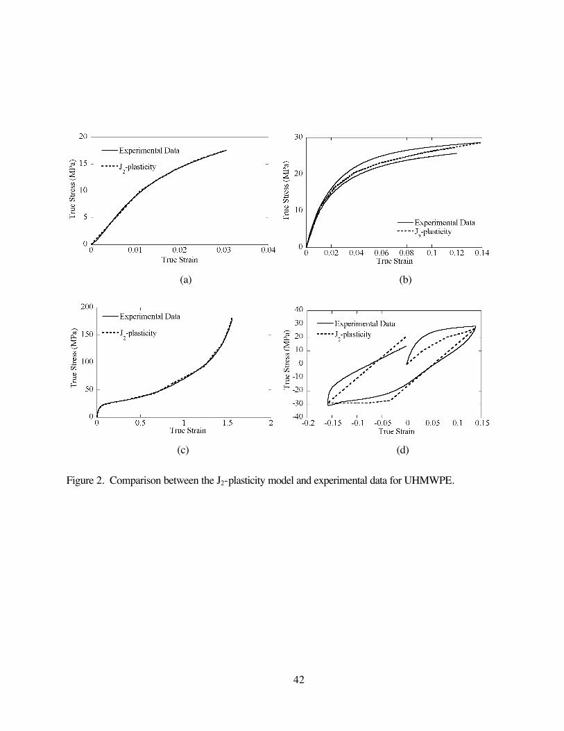
material parameters was limited to 15 or less. As is illustrated in Figure 2, both the small strain and the

large strain experimental data are well predicted, and both sets have an r2-value that exceeds 0.999.

The intermediate strain data is less well predicted since the J2-plasticity model does not incorporate

strain-rate effects. The r2-value of the intermediate strain data is 0.976. Also the cyclic strain data is

rather poorly predicted, having an r2-value of 0.951. The reason for the poor prediction of the cyclic

data is the experimentally observed gradual change in unloading slope after strain reversals, a feature

that the J2-plasticity model cannot capture. As a final test of the J2-plasticity model was also the

combined set of all experimental data evaluated. In this case was one set of optimal parameters used to

predict the experimental data giving a r2-value of the combined set of 0.877.

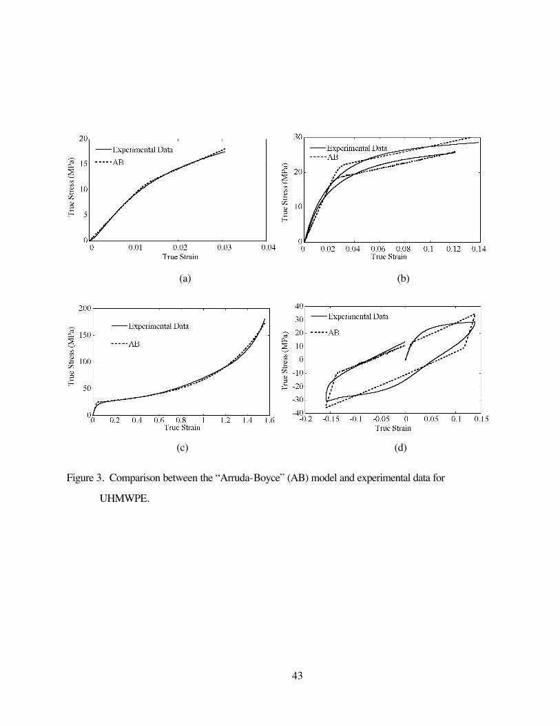
The optimal material parameters for the AB-model are summarized in Table 4 and the predicted

behavior is shown in Figure 3. Similar to the J2-plasticity model, the AB-model is also capable of

predicting both small strain and large strain monotonic loading. The r2-values for these two cases are

0.999 and 0.996, respectively. The behavior under monotonic intermediate strains at different strain

rates is relatively well predicted by the AB-model. In particular, the influence of strain rates is well

captured but the experimentally observed non-linear behavior prior to yield is not captured. This

weakness of the AB-model has been addressed in the HB-model. The prediction of cyclic strain data is

better than the corresponding prediction from the J2-plasticity model, but the quality of the prediction is

still rather crude (having a r2-value of 0.971). Also the prediction of the combined set of experimental

data is better than the J2-plasticity prediction, having a r2-value of 0.966 compared to 0.877 for the J2-

plasticity model.

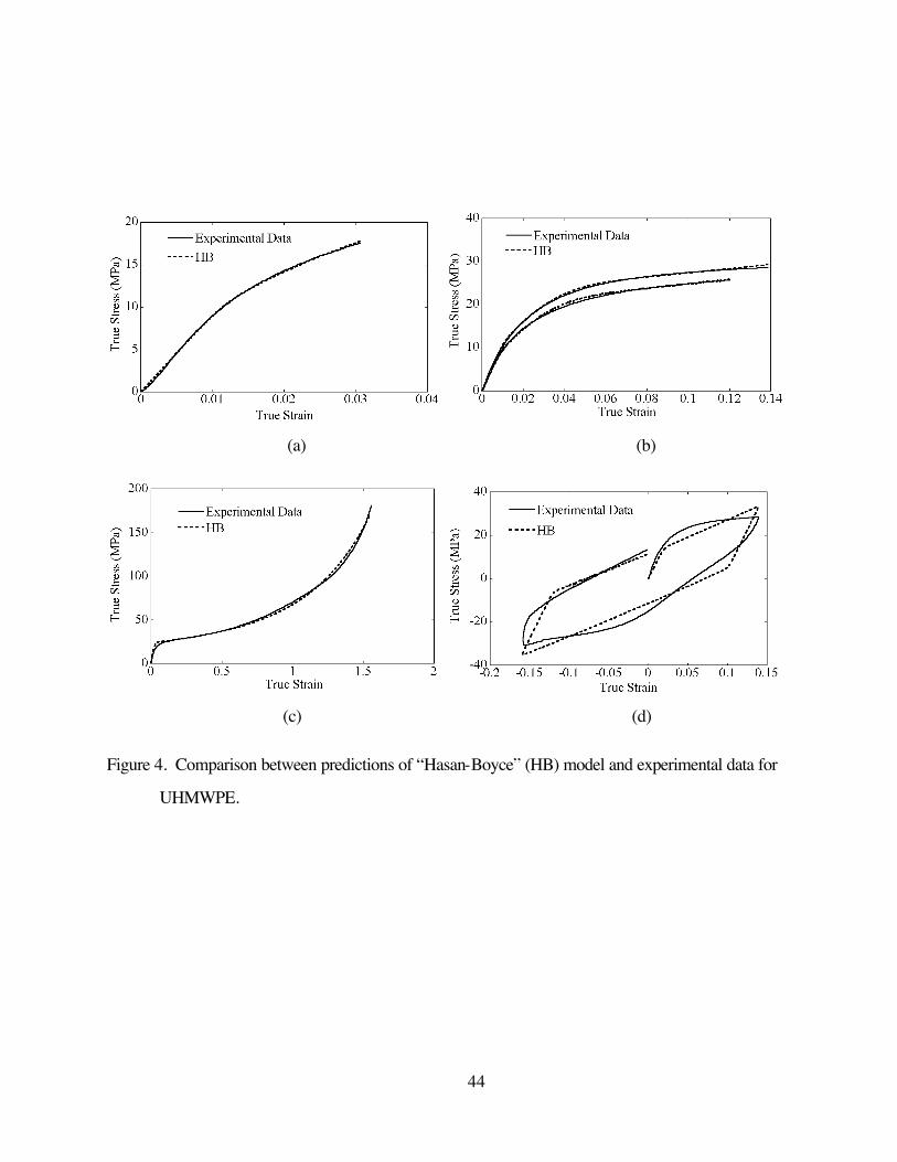
The predicted behavior of the HB-model is depicted in Figure 4 together with the experimental

data. The material parameters used in the HB-model for the different test cases are summarized in

Table 5. As is shown in Figure 4, the HB-model gives good predictions under monotonic loading

12

independent of strain rates and final strain level. For example, the predicted response at intermediate

strain rates is well predicted as indicated by the high r2-value of 0.998. The predicted behavior under

the cyclic strain loading case, however, still only has the same quality as the AB-model. Furthermore,

under cyclic loading conditions the model also behaves very similar to the AB-model in that it captures

the overall magnitudes of the stress response but the gradual transition in behavior between loading and

unloading is modeled well. For this case both the AB and the HB model predictions have r2-values

0.97. As shown in Table 2, the predicted response of the combined set is similar to the AB-model.

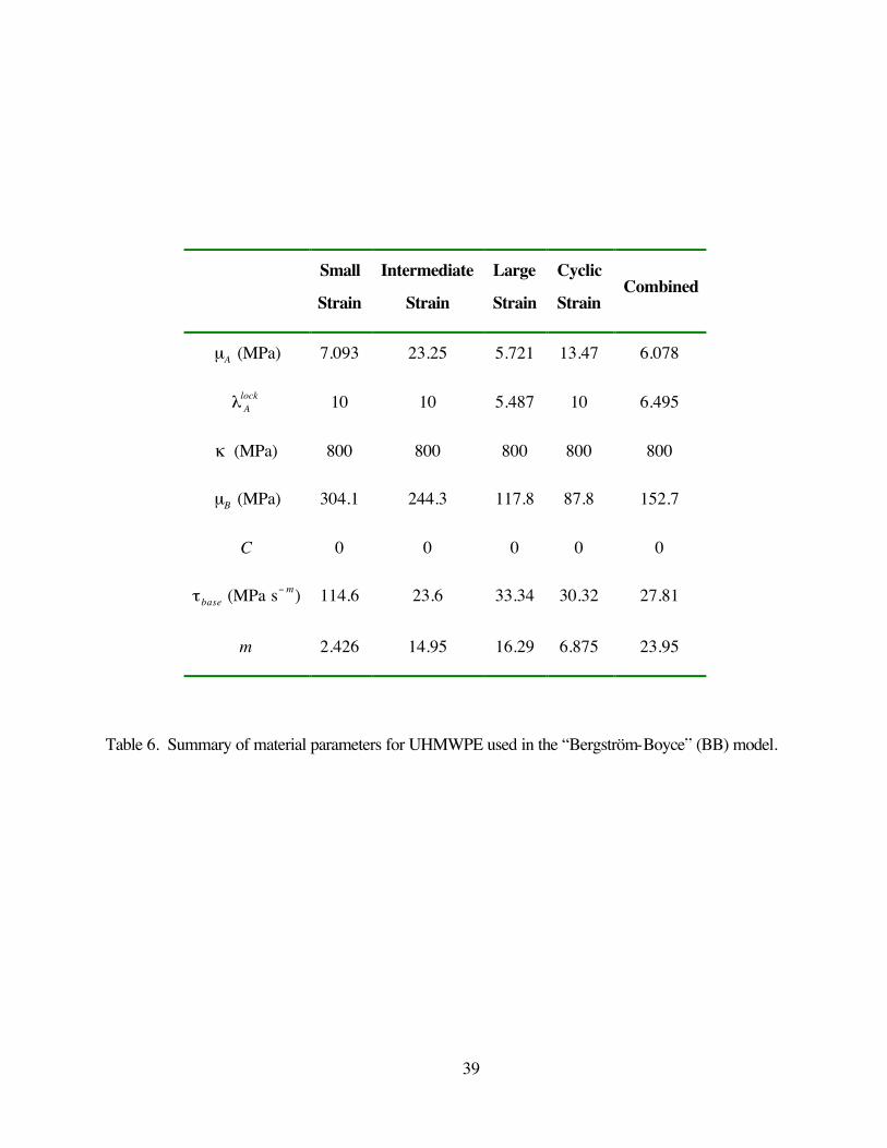
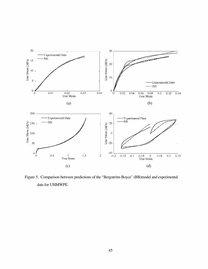
Figure 5 shows that predicted response of the BB-model when subjected to the different strain

data sets. The optimal parameters used in the BB-model are summarized in Table 6. It is interesting to

note that in all test cases the optimal value of the material parameter C is 0. Hence the magnitude of the

plastic flow rate is not dependent on the strain level. This is quite different from elastomeric materials

where the constant C often has a value close to –1 [41]. The quality of the predictions under both

monotonic and cyclic loading conditions are quite similar to the AB-model. The predicted cyclic loading

case, although having a similar r2-value as the AB and HB models, has a different characteristic shape of

the stress-strain response. The combined data set prediction is also similar to the AB and HB

predictions.

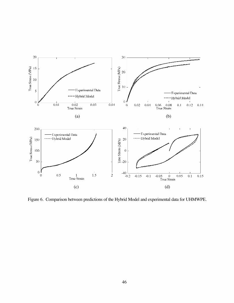
The last model tested was the hybrid model and the predicted results from the model are shown

in Figure 6 and the material parameters used in the different test cases are summarized in Table 7. By

comparing the model predictions with the experimental data it is clear that the hybrid model accurately

predicts all different test cases studied. In all cases the r2-value of the predicted response is 0.997 or

higher.

The most comprehensive test of the different constitutive models is to compare them to the

complete set of experimental data. The results of this comparison are presented in Table 2 and shows

that the hybrid model is clearly the most successful in predicting the behavior of UHMWPE (having a

r2-value of 0.998). Of the other models, the AB, BB, and HB models are about equally good at

predicting the experimental behavior (having an r2-value of about 0.965). Table 2 also shows that the

J2-plasticity model is comparatively poor at predicting the complete set of experimental data of

13

UHMWPE (having a r2-value of 0.613).

Discussion

The results of this study suggest that all five material models tested may be suitable for

describing the mechanical behavior of UHMWPE in monotonic loading at one fixed strain rate. To

predict the behavior at different strain rates the physically inspired polymer models (AB, HB, BB, and

HM) are more suitable, since the J2-plasticity model is strain rate independent. Also, the four physically

inspired polymer models provide better predictions of cyclic loading behavior than the J2-plasticity

model, which is currently the state-of the art material model for UHMWPE. Of the four polymer

models the newly developed hybrid model shows the most promise in describing the mechanical

behavior of UHMWPE. Based on the available data for unirradiated UHMWPE, the hybrid model is

superior to the other models in all test cases. The difference between the quality of the AB, HB, and BB

model predictions is subtle, and based on the results obtained in this study it appears that the added

complexity of the HB model compared to the AB or BB models is not justified based on sufficient

improvements in the predicted results. Since the hybrid model requires a larger number of material

parameters than the AB or BB models it will to some extent be more time consuming to find the optimal

material properties for a new material. Thus, depending on the application, one of the simpler theories

(e.g. AB or BB) may provide an adequate description of the mechanical behavior of virgin UHMWPE,

even though the hybrid model appears to be the most powerful.

The determination of the material parameters used in the constitutive models examined in this

work can be a challenging task. Since none of the models under normal conditions can perfectly predict

the discrete experimental data, for example due to experimental errors, a unique solution does not exist.

Mathematically, the task of finding the material parameters can be regarded as an optimization problem.

This means that the actual method of determining the material parameters, whether each parameter is

isolated and determined individually or if the parameters are found through a computer algorithm is of

secondary interest relative to the issue of validation. The only way to determine if a particular set of

material parameters is relevant or not is by comparing the predictions of the resulting model with

14

experimental data. The model parameters may be considered to be validated if they can be used to

successfully predict mechanical behavior under different loading conditions than that under which they

were determined.

The approach used in this work to find the material parameters needed in the different

constitutive models was based on two techniques. First an initial set of parameters was determined

using insight from the models and how they work. For example, in the AB, HB, and HM models the

initial slope of the experimentally determined stress-strain response directly gives the Young’s modulus

of network e. Similar “graphical” techniques can be used to determine the majority of the needed

parameters [41,47]. A few of the parameters, however, are difficult to obtain in this manner and it is

therefore often common to have to use known values of similar materials in combination with empirical

estimates. The second technique used in this work to determine the material parameters was based on

a numerical optimization algorithm. Note that to use this approach effectively it is still necessary to use a

good set of starting values of the material parameters. The advantage of this method is that it reduces

the empiricism associated with the parameter estimation.

An important motivation for using a physically based constitutive theory to represent the

mechanical behavior of a polymer is that the response of the material is then likely to be predictable

under a wider range of loading conditions. These conditions can include complexities such as multiaxial

deformation states, cyclic loading histories, and arbitrary changes in strain rate and temperature. By

incorporating the proper physics into the theory, the model can be calibrated through the use of a

relatively small number of simple mechanical tests. Again, this approach has advantages over methods

that simply attempt to mathematically parameterize or “fit” the material behavior to a large number of

experiments performed under various loading/environmental conditions in that it can reliably be used to

predict behavior outside of the conditions from which the parameters are determined. A multiaxial

deformation comparison between the different constitutive theories examined in this paper is under way

and will be reported in a later communication.

The data sets used in this study were derived from physical experiments on a single type of

UHMWPE (GUR 4150 HP), which, until recently, was commonly used to fabricate total joint

15

replacement components [1]. GUR 4150 HP contains calcium stearate, a processing and whitening aid

[1]. Recently, orthopedic manufacturers have shifted to grades of UHMWPE that do not contain added

calcium stearate. Because of its high melt viscosity, UHMWPE is processed using ram extrusion or

compression molding. These different processing methods may influence the mechanical properties of

the polymer because of their different thermal and pressure histories [1]. Furthermore, prior to

implantation, UHMWPE is commonly subjected to ionizing radiation (gamma and electron beam) for

sterilization and crosslinking of the polymer for improved wear resistance [1]. Irradiation doses may

range from 25 to 40 kGy for sterilization and up to 100 kGy for crosslinking modifications to the

polymer. All of these factors can be expected to result in changes to the mechanical behavior of

UHMWPE, and will require an extensive testing program to quantify the effects of resin grade,

processing route, and radiation exposure on the constitutive model. Thus, the data for unirradiated, ram

extruded GUR 4150 HP relied upon for the present study provided the necessary initial basis for

verification of the constitutive theories, but a more extensive database based on different forms of

UHMWPE will be needed for comprehensive validation of our approach. Therefore, studies are

currently underway to determine whether the constitutive theories outlined herein are sufficiently general

to be applicable for a wide range of UHMWPE materials used in total joint replacements.

Acknowledgements

Special thanks to Professor Mary Boyce from the Massachusetts Institute of Technology and to

Tim Harrigan, Exponent, Inc., for many helpful discussions. Supported by NIH Grant 1 R01 AR 47192

and by a research grant from Howmedica Osteonics Corp.

16

Appendix A. List of Symbols

α Power exponent used in the hybrid model

ε Scalar effective strain

ε f Limiting scalar effective strain

1 2ˆ ˆ ˆ, ,ε ε ε Reference scalar effective strain

φ x( ) Distribution function for activation energies

pγ& Magnitude of plastic flow rate

0γ& Pre-exponential factor

iγ& Combined pre-exponential factor

Bγ& Magnitude of plastic flow rate of network B

κ Bulk modulus

λe Second Lamé constant

λ lockp Locking chain stretch of the back stress network

λ Alock Locking chain stretch of network A

λp Effective chain stretch of back stress network

λ* Effective chain stretch

pBλ Effective chain stretch of the viscous component of the deformation of network

B

L−1 x( ) Inverse Langevin function

µe Elastic shear modulus

µp Shear modulus of the back stress network

µA Initial shear modulus of network A

µB Shear modulus of network B

17

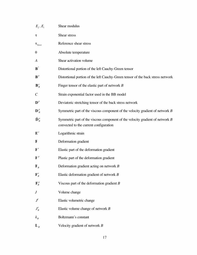
Ef , Ei Shear modulus

τ Shear stress

τbase Reference shear stress

θ Absolute temperature

A Shear activation volume

B* Distortional portion of the left Cauchy-Green tensor

B p Distortional portion of the left Cauchy-Green tensor of the back stress network

eBB Finger tensor of the elastic part of network B

C Strain exponential factor used in the BB model

D p Deviatoric stretching tensor of the back stress network

D Bp Symmetric part of the viscous component of the velocity gradient of network B

pBD% Symmetric part of the viscous component of the velocity gradient of network B

convected to the current configuration

E e Logarithmic strain

F Deformation gradient

F e Elastic part of the deformation gradient

F p Plastic part of the deformation gradient

FB Deformation gradient acting on network B

FBe Elastic deformation gradient of network B

pBF Viscous part of the deformation gradient B

J Volume change

Je Elastic volumetric change

JBe Elastic volume change of network B

kB Boltzmann’s constant

LB Velocity gradient of network B

18

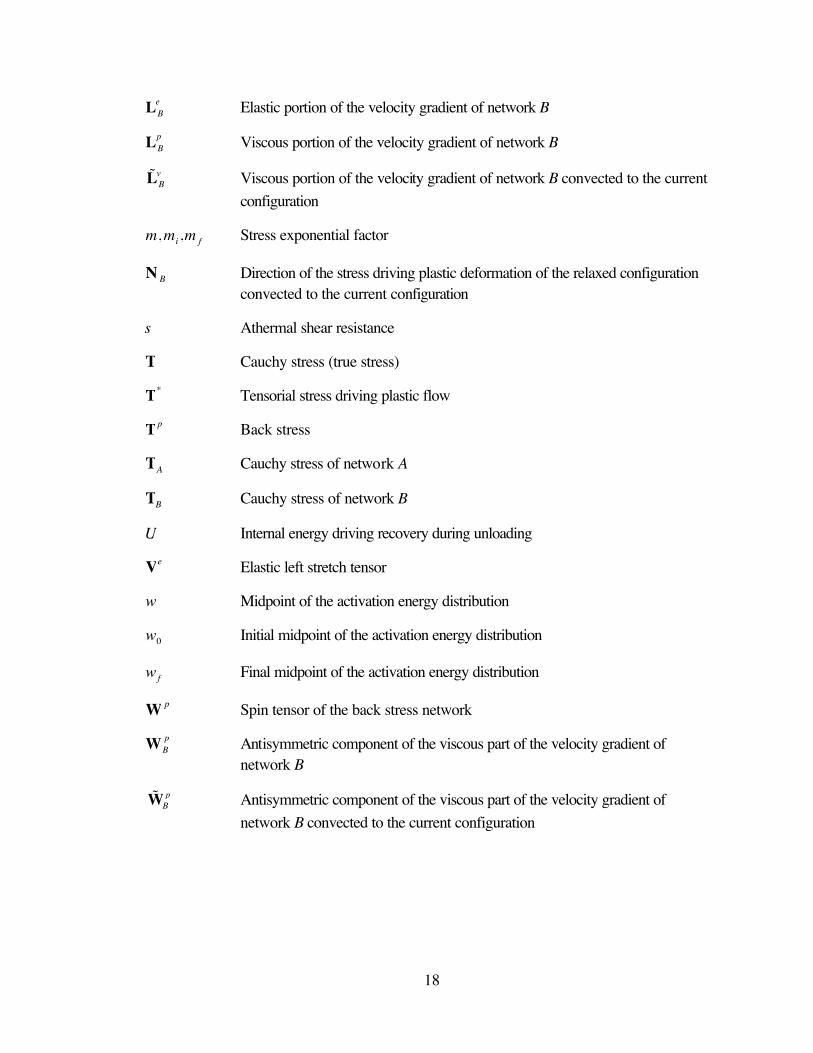
LBe Elastic portion of the velocity gradient of network B

LBp Viscous portion of the velocity gradient of network B

vBL% Viscous portion of the velocity gradient of network B convected to the current

configuration

m, mi ,m f Stress exponential factor

N B Direction of the stress driving plastic deformation of the relaxed configuration convected to the current configuration

s Athermal shear resistance

T Cauchy stress (true stress)

T* Tensorial stress driving plastic flow

T p Back stress

TA Cauchy stress of network A

TB Cauchy stress of network B

U Internal energy driving recovery during unloading

Ve Elastic left stretch tensor

w Midpoint of the activation energy distribution

w0 Initial midpoint of the activation energy distribution

wf Final midpoint of the activation energy distribution

W p Spin tensor of the back stress network

WBp Antisymmetric component of the viscous part of the velocity gradient of

network B

pBW% Antisymmetric component of the viscous part of the velocity gradient of

network B convected to the current configuration

19

Appendix B. Constitutive Models for Polymers

This section summarizes four different constitutive theories than can be used to predict the

mechanical behavior of UHMWPE. The models examined are the J2-plasticity model, the Bergstrom-

Boyce model, the Arruda-Boyce model, and the Hasan-Boyce model.

Isotropic (J2) Plasticity

One example of incorporating considerations of the physics of material behavior into a

constitutive model is the use of classical metal plasticity theory. This theory, often referred to as J2-flow

theory, is based on Mises yield surface with an associated flow rule, followed by rate-independent

isotropic hardening. Physically, plastic flow in metals is a result of dislocation motion, a mechanism

known to be driven by shear stresses and being insensitive to hydrostatic pressure. One consequence

of this is that metals are observed to be nearly incompressible during plastic deformation. The

incorporation of these ideas into the theory allows it to capture the essential physics of this class of

materials and gives it good predictive power. The necessary material parameters needed to predict the

behavior under arbitrary states of deformation can be obtained from uniaxial deformation data.

For materials where the basic physics of deformation is different from that described above, the

J2-plasticity model often performs quite poorly when applied to complex loading conditions. This

occurs, for example, in material systems that develop texture or other forms of anisotropy during

deformation. The mechanisms governing the plastic deformation for polymeric materials are quite

different from those of metals. For example, the deformation resistance of amorphous polymers in the

glassy regime is determined by a combination of thermally activated segmental rearrangements [48]

(primarily responsible for the plastic behavior at small to moderate strains) and orientation induced strain

hardening due to polymer chain stretching and alignment (primarily responsible for the deformation

resistance at large strains [49]). In addition, in the case of semi-crystalline polymers such as

UHMWPE, mechanisms associated with crystallographic slip, twinning, martensitic transformations, and

crystallite/lamellar rotation also play a role [22].

20

The Arruda-Boyce (AB) Model

The Arruda-Boyce (AB) model was developed [42,50,51] for predicting the large strain, time-

and temperature-dependent response of glassy polymers. The behavior of this class of materials when

subjected to gradually increasing loads is characterized by an initial linear elastic response followed by

yielding and then strain hardening at large deformations. This evolution in material response with applied

loads is directly incorporated into the AB model.

In the AB framework, the total deformation gradient is decomposed into elastic and plastic

components, F = F eF p . As is shown in the one-dimensional rheological representation in Figure B1,

this decomposition can be interpreted as two networks acting in series: one elastic network (e) and one

plastic network (p). Using this decomposition of the deformation gradient the Cauchy stress can be

calculated from the linear elastic relationship:

T =1J e 2 µeE e + λe tr E e[ ]1( ), (B.1)

where E e = ln[ Ve ] is the logarithmic true strain, Je = det[Fe] , and µe ,λe are Lamé’s constants. The

stress driving the plastic flow is given by the tensorial difference between the total stress and the

convected back stress

* 1 e p eTeJ

= −T T F T F , (B.2)

where the deviatoric back stress is given by the incompressible 8-chain model which can be written

[45,52]

Tp =µp

λp

L−1 λp

λlockp

L−1 1λlock

p

dev Bp[ ] (B.3)

with µp ,λlockp being physically motivated material constants, B p = F pF pT , ( )tr / 3p pλ = B the

effective chain stretch based on the eight-chain topology assumption, and L(x) = coth( x) −1/ x the

Langevin function.

21

In the original work [42,50,51] the plastic flow rate was given by

5/6

0 exp 1p

B

Ask s

τγ γ

θ

− = − & & , (B.4)

where 0 , ,A sγ& are material constants, kB is Boltzmann’s constant, and θ is the absolute temperature.

It has been shown by Hasan and Boyce [40] that the difference in behavior between a stress exponent

of 5/6 and 1 is very small. By taking the stress exponent to be 1 and grouping material constants

together the expression for the plastic flow rate can be simplified to

exp exppo i

base base

sτ τγ γ

τ τγ

−= =

& && , (B.5)

where /base Bk Aτ θ= , and ( )0 exp /i basesγ γ τ= −& & , which is the expression used here. The focus of the

current work is on isothermal deformation histories, to explicitly include temperature effects the

parameter τbase can be replaced by kBθ / A . The scalar equivalent stress τ is here taken as the

Frobenius norm of the deviatoric part of the driving stress τ = || dev T*[ ]||F , where || A ||F = (AijAij)1/ 2 .

The rate of plastic deformation is given by

*D devp

p γ

τ = T

& (B.6)

and the plastic spin is taken to be zero [53], i.e. 0p =W , which uniquely specifies the rate kinematics.

Note that the original Boyce model also allows for modeling of strain softening through an

evolution equation of the athermal shear resistance, s. As will be shown in the Results section, however,

UHMWPE does not exhibit strain softening and this extra feature of the constitutive model is

unnecessary to model UHMWPE.

The Hasan-Boyce (HB) Model

The Hasan-Boyce (HB) model is an extension of the Arruda-Boyce model and is based on the

same kinematic framework. The main difference between the two models is that in the HB approach a

distribution and evolution of activation energies is incorporated into the expression for the magnitude of

22

the plastic deformation rate ( pγ& ). To illustrate the approach taken in the HB model consider the

following expression for the plastic deformation rate:

( )0 exp .p

base

xx dx

τγ γ φ

τ

+∞

−∞

−=

∫& & (B.7)

Note that this equation becomes identical to the original Equation (B.5) if ( ) ( )x x sφ δ= − . The

function ( )xφ can here be interpreted as a probability distribution function for the athermal shear

resistance as a function of stress. In the Arruda-Boyce model there was only one shear resistance, s ,

here captured with the delta function ( ) ( )x x sφ δ= − . Hasan and Boyce argue [40] that a more

physically-based distribution in shear resistances is given by

( )

( )

1

2

1 1

1 2 2

3sin , where , if 43

( ) sin , where , if 4

0, otherwise

e x s w s w x sw

x C e x s w s x s ww

π

πφ

Λ

Λ

Λ Λ = − + − < <

= Λ Λ = − − < < +

(B.8)

where

( )1

3( )4 2exp(3 /4) 1

C ww

π

π=

+ (B.9)

is chosen such that the area under the distribution function becomes unity.

By including both forward and backward flow in addition to the storage of inelastic energy the

expression for the plastic deformation rate proposed by Hasan and Boyce can be written

0( ) ( )

( ) exp exp .p

base base

x x Ux dx

τ τγ γ φ

τ τ

+∞

−∞

− − − + + = −

∫& & (B.10)

By integrating this equation and only consider dominant terms the following approximation can be

obtained (see Appendix C for details)

23

( 2 ) /

2

1exp

1 1.2( / )

baseUp

ibase base

e ww

τ τ τγ γ

τ τ

− + − +≈ +

& & . (B.11)

In the original HB model, the parameters U, s, and w were all evolved with the applied deformation

through a set of coupled non-linear differential equations. Besides being computationally expensive, this

approach also makes it difficult to systematically obtain the material parameters used when evolving the

ordinary differential equations (ODEs). Instead of evolving the internal state variables through a set of

ODEs, it is proposed here to use one explicit algebraic equation to capture the evolving state. This

equation determines the width of the probability distribution function as a function of the applied strain,

and thereby fulfills the same functionality as the original HB approach:

( )0 0

ˆexp( / ) 1 , if ˆexp( / ) 1

, otherwise

f ff

f

w w ww

w

ε εε ε

ε ε

− −+ − ≤

− −=

(B.12)

where || ||pFε = E . Using this expression the equation for the plastic strain rate can be simplified to

2 /

2

1exp

1 1.2( / )

basep

ibase base

e ww

τ τ τγ γ

τ τ

− − += +

& & (B.13)

Note that the influence of the internal energy U is not directly taken into account as in the original HB

model, instead the internal energy is here implicitly considered through the width of the probability

distribution function for the activation energy. The simplifications used in obtaining Equation (B.13)

makes the proposed model easier to use and more computationally efficient then the original HB-model.

At the same time, however, the proposed model is less powerful than the original HB framework.

The Bergström-Boyce (BB) Model

Another recently developed model is the Bergström-Boyce (BB) model [41]. This model was

developed for predicting time-dependence and hysteresis of crosslinked polymers above their glass

transition temperature, i.e. elastomeric materials. Although UHMWPE is not an elastomeric material,

there are reasons why this model might still predict the behavior of UHMWPE. As a characteristic of

elastomers, the glass transition temperature of UHMWPE is rather low (Tg = −80°C) compared to

24

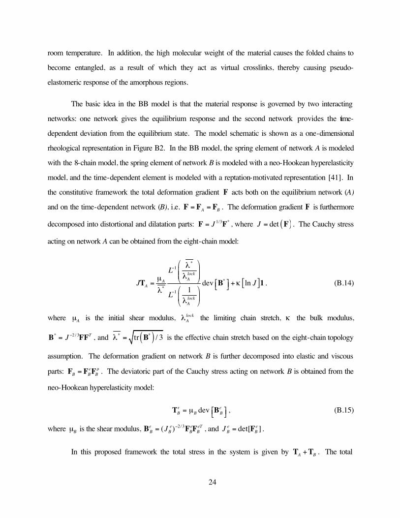
room temperature. In addition, the high molecular weight of the material causes the folded chains to

become entangled, as a result of which they act as virtual crosslinks, thereby causing pseudo-

elastomeric response of the amorphous regions.

The basic idea in the BB model is that the material response is governed by two interacting

networks: one network gives the equilibrium response and the second network provides the time-

dependent deviation from the equilibrium state. The model schematic is shown as a one-dimensional

rheological representation in Figure B2. In the BB model, the spring element of network A is modeled

with the 8-chain model, the spring element of network B is modeled with a neo-Hookean hyperelasticity

model, and the time-dependent element is modeled with a reptation-motivated representation [41]. In

the constitutive framework the total deformation gradient F acts both on the equilibrium network (A)

and on the time-dependent network (B), i.e. A B= =F F F . The deformation gradient F is furthermore

decomposed into distortional and dilatation parts: 1/3 *J=F F , where ( )detJ = F . The Cauchy stress

acting on network A can be obtained from the eight-chain model:

[ ]

*1

**

1

dev ln1

lockAA

A

lockA

LJ J

L

λλµ

κλ

λ

−

−

= +

T B 1 . (B.14)

where µA is the initial shear modulus, lockAλ the limiting chain stretch, κ the bulk modulus,

* 2 / 3 TJ −=B FF , and ( )* *tr / 3λ = B is the effective chain stretch based on the eight-chain topology

assumption. The deformation gradient on network B is further decomposed into elastic and viscous

parts: e pB B B=F F F . The deviatoric part of the Cauchy stress acting on network B is obtained from the

neo-Hookean hyperelasticity model:

dev eB B Bµ′ = T B , (B.15)

where µB is the shear modulus, 2/3( )e e e eTB B B BJ −=B F F , and det[ ]e e

B BJ = F .

In this proposed framework the total stress in the system is given by A B+T T . The total

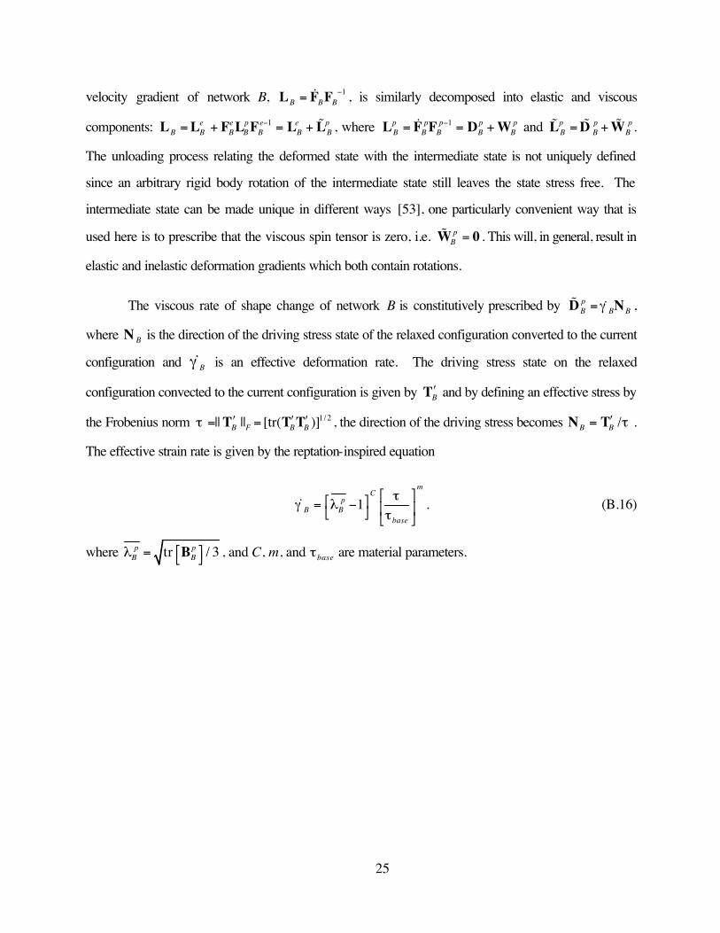
25

velocity gradient of network B, 1B B B

−=L F F& , is similarly decomposed into elastic and viscous

components: 1e e p e e pB B B B B B B

−= + = +L L F L F L L% , where 1p p p p pB B B B B

−= = +L F F D W& and p p pB B B= +L D W% % % .

The unloading process relating the deformed state with the intermediate state is not uniquely defined

since an arbitrary rigid body rotation of the intermediate state still leaves the state stress free. The

intermediate state can be made unique in different ways [53], one particularly convenient way that is

used here is to prescribe that the viscous spin tensor is zero, i.e. pB =W 0% . This will, in general, result in

elastic and inelastic deformation gradients which both contain rotations.

The viscous rate of shape change of network B is constitutively prescribed by pB B Bγ=D N% & ,

where N B is the direction of the driving stress state of the relaxed configuration converted to the current

configuration and Bγ& is an effective deformation rate. The driving stress state on the relaxed

configuration convected to the current configuration is given by B′T and by defining an effective stress by

the Frobenius norm 1/2|| || [tr( )]B F B Bτ ′ ′ ′= =T T T , the direction of the driving stress becomes /B B τ′=N T .

The effective strain rate is given by the reptation-inspired equation

1m

Cp

B Bbase

τγ λ

τ

= − & . (B.16)

where tr / 3p pB Bλ = B , and C, m, and τbase are material parameters.

26

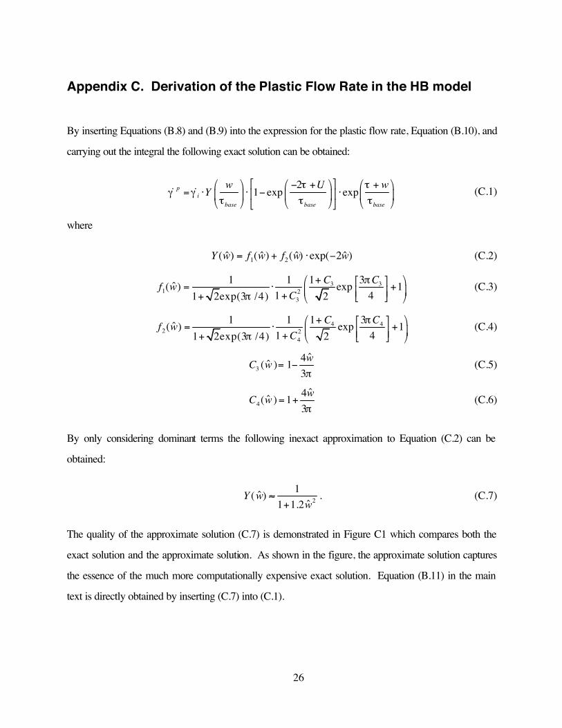
Appendix C. Derivation of the Plastic Flow Rate in the HB model

By inserting Equations (B.8) and (B.9) into the expression for the plastic flow rate, Equation (B.10), and

carrying out the integral the following exact solution can be obtained:

21 exp expp

ibase base base

w U wY

τ τγ γ

τ τ τ

− + += ⋅ ⋅ − ⋅

& & (C.1)

where

1 2ˆ ˆ ˆ ˆ( ) ( ) ( ) exp( 2 )Y w f w f w w= + ⋅ − (C.2)

3 31 2

3

1 31 1ˆ( ) exp 11 41 2exp(3 /4) 2

C Cf wC

π

π

+ = ⋅ + ++ (C.3)

4 42 2

4

1 1 1 3ˆ( ) exp 11 41 2exp(3 /4) 2

C Cf wC

π

π

+ = ⋅ + ++ (C.4)

3ˆ4ˆ( ) 1

3wC wπ

= − (C.5)

4ˆ4ˆ( ) 1

3wC wπ

= + (C.6)

By only considering dominant terms the following inexact approximation to Equation (C.2) can be

obtained:

21ˆ( )

ˆ1 1.2Y w

w≈

+. (C.7)

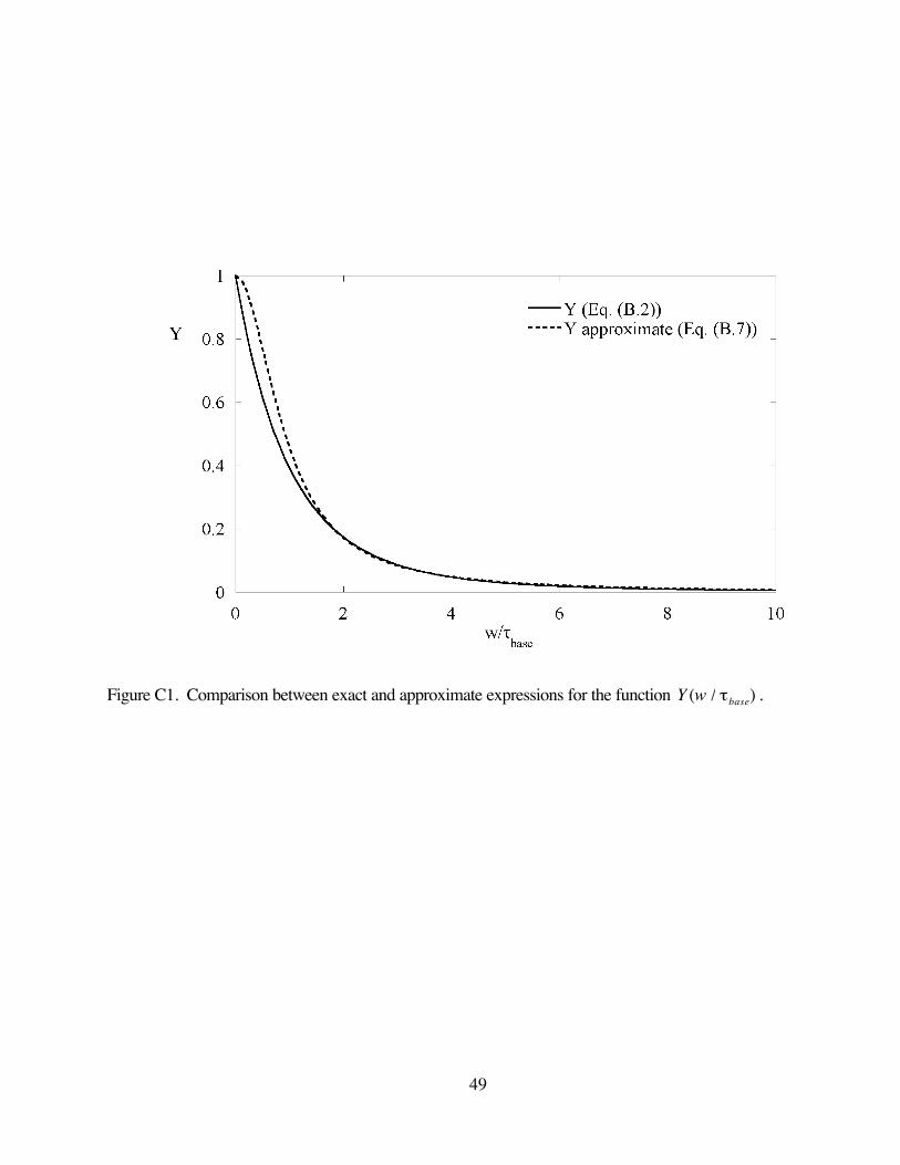
The quality of the approximate solution (C.7) is demonstrated in Figure C1 which compares both the

exact solution and the approximate solution. As shown in the figure, the approximate solution captures

the essence of the much more computationally expensive exact solution. Equation (B.11) in the main

text is directly obtained by inserting (C.7) into (C.1).

27

References

[1] Kurtz SM, Muratoglu OK, Evans M, Edidin AA. Advances in the processing, sterilization, and

crosslinking of ultra- high molecular weight polyethylene for total joint arthroplasty. Biomaterials

1999;20: 1659-1688.

[2] Orthopaedic Products. In: R.C. Smith, M.A. Geier, J. Reno, J. Sarasohn-Kahn, editors. 1999-

2000 Medical & Healthcare Marketplace Guide. New York: IDD Enterprises, L.P., 1998.

[3] Dannenmaier WC, Haynes DW, Nelson CL. Granulomatous reaction and cystic bony destruction

associated with high wear rates in a total knee prosthesis. Clin Orthop Rel Res 1985;198: 224-

230.

[4] Howie DW, Vernon-Roberts B, Oakeshott R, Manthey B. A rat model of resorption of bone at

the cement-bone interface in the presence of polyethylene wear particles. J Bone Joint Surg Am

1988;70A: 257-263.

[5] Mirra JM, Marder RA, Amstutz HC. The pathology of failed total joint arthroplasty. Clin Orthop

Rel Res 1982;170: 175-183.

[6] Wang A, Stark C, Dumbleton JH. Role of cyclic plastic deformation in the wear of UHMWPE

acetabular cups. J Biomed Mater Res 1995;29: 619-626.

[7] Jasty M, Goetz DD, Bragdon CR, Lee KR, Hanson AE, Elder JR, Harris WH. Wear of

polyethylene acetabular components in total hip arthroplasty. An analysis of one hundred and

twenty-eight components retrieved at autopsy or revision operations. J Bone Joint Surg Am

1997;79: 349-358.

[8] Pascaud RS, Evans WT. Critical assessment of methods for evaluating Jic for a medical grade

ultra-high molecular weight polyethylene. Polymer Eng. Sci 1997;37: 11.

[9] Wrona M, Mayor MB, Collier JP, Jensen RE. The correlation between fusion defects and

28

damage in tibial polyethylene bearings. Clin Orthop 1994;299: 92-103.

[10] Blunn GW, Lilley PA, Walker PS. Variability of the wear of ultra high molecular weight

polyethylene in simulated TKR. Transactions of the 40th Orthopedic Research Society 1994;

177.

[11] Bartczak Z, Cohen RE, Argon AS. Evolution of the crystalline texture of high-density

polyethylene during uniaxial compression. Macromolecules 1992;25: 4692-4704.

[12] G'Sell C, Jonas JJ. Determination of the plastic behaviour of solid polymers at constant true strain

rate. J. Materials Sci. 1979;14: 583.

[13] G'Sell C, Boni S, Shrivastava S. Application of the plane simple shear test for determination of the

plastic deformation of solid polymers at large strains. J. Materials Sci. 1983;18: 903-918.

[14] G'Sell C, Hiver JM, Dahoun A, Souahi A. Video-controlled tensile testing of polymers and metals

beyond the necking point. J Mat Sci 1992;27: 5031-5039.

[15] G'Sell C, Dahoun A. Evolution of microstructure in semi-crystalline polymers under large plastic

deformations. Mat Sci Eng 1994;A175: 183-199.

[16] G'Sell C, Paysant-Le Roux B, Dahoun A, Cunat C, von Stebut J, Mainard D. Plastic behaviour

and resistance to wear of ultra-high molecular weight polyethylene. Deformation, Yield and

Fracture of Polymers 1997; 57-60.

[17] Galeski A, Bartczak Z, Cohen RE, Argon AS. Morphological alterations during texture-

producing plastic plane strain compression of high density polyethylene. Macromolecules

1992;25: 5705-5718.

[18] Katagiri T, Sugimoto M, Nakanishi E, Hibi S. Orientation behavior of crystallites in cylindrical

polyethylene rods under tension-torsion combined stress. Polymer 1993;34: 487-493.

[19] Kitagawa M, Onoda T, Mizutani K. Stress-strain behavior at finite strains for various strain paths

in polyethylene. J. Materials Sci. 1992;27: 13-23.

29

[20] Kitagawa M, Zhou D, Qiu J. Stress-strain curves for solid polymers. Polymer Eng. Sci. 1995;35:

1725-1732.

[21] Lee BJ, Argon AS, Parks DM, Ahzi S, Bartczak Z. Simulation of large strain plastic deformation

and texture evolution in high density polyethylene. Polymer 1993;34: 3555-3575.

[22] Lin L, Argon AS. Review: Structure and plastic deformation of polyethylene. J. Mat. Sci.

1994;29: 294-323.

[23] Meinel G, Peterlin A. Plastic deformation of polyethylene II. Change in mechanical properties

during drawing. J Polymer Sci 1971;9: 67-83.

[24] Peterlin A. Molecular model of drawing polyethylene. J Polymer Sci 1971;6: 490-508.

[25] Rodriguez-Cabello JC, Merion JC, Jawhari T, Pastor JM. Rheo-optical Raman study of chain

deformation in uniaxially stretched bulk polyethylene. Polymer 1995;36: 4233-4238.

[26] Vincent PI. The necking and cold-drawing of rigid plastics. Polymer 1960;1: 7-19.

[27] Bartel DL, Rawlinson JJ, Burstein AH, Ranawat CS, Flynn WF, Jr. Stresses in polyethylene

components of contemporary total knee replacements. Clin Orthop 1995;317: 76-82.

[28] Kurtz SM, Jewett CW, Crane D, Pruitt L, Foulds JR, Edidin AA. Ultimate properties and

crystalline morphology of ultra-high molecular weight polyethylene during uniaxial and biaxial

tension. Trans 24th Soc Biomater 1998; 125.

[29] Kurtz SM, Rimnac CM, Santner TJ, Bartel DL. Exponential model for the tensile true stress-

strain behavior of as-irradiated and oxidatively degraded ultra high molecular weight polyethylene.

J Orthop Res 1996;14: 755-761.

[30] Kurtz SM, Bartel DL, Rimnac CM. Post-irradiation aging affects the stresses and strains in

UHMWPE components for total joint replacement. Clin Orthop 1998;350: 209-220.

[31] Scifert CF, Brown TD, Pedersen DR, Callaghan JJ. Effects of acetabular component lip design

on dislocation resistance in THA. Trans ASME Bioengineering (Winter) 1997; 295-296.

30

[32] Petrella AJ, Rubash HE, Miller MC. The effect of femoral component rotation on the stresses in

an UHMWPE patellar prosthesis-a finite element study. Trans ASME Bioengineering (Winter)

1997; 309-310.

[33] Elbert K, Bartel D, Wright T. The effect of conformity on stresses in dome-shaped polyethylene

patellar components. Clin Orthop 1995;317: 71-75.

[34] Hughes TJR. Numerical implementation of constitutive models: rate-independent deviatoric

plasticity. In: S. Nemat-Nasser, R.J. Asaro, G.A. Hegemier, editors. Theoretical Foundation for

Large-Scale Computations for Nonlinear Material Behavior. Dordrecht: Martinus Nijhoff

Publishers, 1984.

[35] Wright TM, Gunsallus KL, Rimnac CM, Bartel DL, Klein RW. Design considerations from an

acetabular component made from an enhanced form of ultra high molecular weight polyethylene.

Transactions of the 37th Orthopedic Research Society 1991; 248.

[36] Kurtz SM, Pruitt L, Jewett CW, Crawford RP, Crane DJ, Edidin AA. The yielding, plastic flow,

and fracture behavior of ultra-high molecular weight polyethylene used in total joint replacements.

Biomaterials 1998;19: 1989-2003.

[37] Bartel DL, Bicknell VL, Wright TM. The effect of conformity, thickness, and material on stresses

in ultra-high molecular weight components for total joint replacement. J Bone Joint Surg [Am]

1986;68: 1041-1051.

[38] Estupiñán JA, Bartel DL, Wright TM. Residual stresses in ultra-high molecular weight

polyethylene loaded cyclically by a ridid moving indenter in nonconforming geometries. J Orthop

Res 1998;16: 80-88.

[39] Ishikawa H, Fujiki H, Yasuda K. Contact analysis of ultrahigh molecular weight polyethylene

articular plate in artificial knee joint during gait movement. J Biomech Eng 1996;118: 377-386.

[40] Hasan OA, Boyce MC. A Constitutive Model for the Nonlinear Viscoplastic Behavior of Glassy

Polymers. Polym. Eng. Sci. 1995;35: 331-344.

31

[41] Bergström JS, Boyce MC. Constitutive Modelling of the Large Strain Time-Dependent Behavior

of Elastomers. J. Mech. Phys. Solids 1998;46: 931-954.

[42] Arruda EM, Boyce MC. Evolution of Plastic Anisotropy in Amorphous Polymers during Finite

Straining. Int. J. Plast. 1993;9: 697-720.

[43] Gurtin ME. An introduction to continuum mechanics (Academic Press, Inc., 1981).

[44] Silhavý M. The mechanics and thermodynamics of continuous media (Springer-Verlag, 1997).

[45] Arruda EM, Boyce MC. A Three-Dimensional Constitutive Model for the Large Stretch

Behavior of Rubber Elastic Materials. J. Mech. Phys. Solids 1993;41: 389-412.

[46] Krzypow DJ, Rimnac CM. Cyclic steady state stress-strain behavior of UHMW polyethylene [In

Process Citation]. Biomaterials 2000;21: 2081-2087.

[47] Arruda EM, Boyce MC. Effects of strain rate, temperature and thermomechanical coupling on the

finite strain deformation of glassy polymers. Mech. Mater. 1995;19: 193-212.

[48] Argon AS. A theory for the low temperature plastic deformation of glassy polymers. Philos. Mag.

1973;28: 839-865.

[49] Haward RN. Physics of Glassy Polymers. Appl Sci. Pub. 1973; Essex.

[50] Boyce MC, Argon AS, Parks DM. Mechanical Properties of Compliant Particles Effective in

Toughening Glassy Polymers. Polymer 1987;28: 1680-1694.

[51] Boyce MC, Parks DM, Argon AS. Large Inelastic Deformation of Glassy Polymers, Part I: Rate-

Dependent Constitutive Model. Mech. Mater. 1988;7: 15-33.

[52] Bergström JS, Boyce MC. Large strain time-dependent behavior of filled elastomers. Mech.

Mater. 2000;32: 627-644.

[53] Boyce MC, Weber GG, Parks DM. On the Kinematics of Finite Strain Plasticity. J. Mech. Phys.

Solids 1989;37: 647-665.

32

Figure Captions

Figure 1. Rheological representation of the “Hybrid Model” (HM). Network e gives the elastic

response and network p gives the visco-plastic response.

Figure 2. Comparison between the J2-plasticity model and experimental data for UHMWPE.

Figure 3. Comparison between the “Arruda-Boyce” (AB) model and experimental data for

UHMWPE.

Figure 4. Comparison between predictions of “Hasan-Boyce” (HB) model and experimental data for

UHMWPE.

Figure 5. Comparison between predictions of the “Bergström-Boyce” (BB)model and experimental

data for UHMWPE.

Figure 6. Comparison between predictions of the Hybrid Model and experimental data for UHMWPE.

Figure B1. Rheological representation of the “Arruda-Boyce” (AB) model. Network e gives the elastic

response and network p gives the visco-plastic response.

Figure B2. Rheological representation of the “Bergström Boyce” (BB) model. Spring 1 gives the

equilibrium response and spring 2 and dashpot 3 give the time-dependent response.

Figure C1. Comparison between exact and approximate expressions for the function Y (w / τbase) .

33

Table Captions

Table 1. Experimental data from previous studies used to validate the constitutive theories for

UHMWPE [36,46].

Table 2. Performance comparison of the different material models (“Arruda-Boyce”, “Hasan-Boyce”,

“Bergström-Boyce”, and “Hybrid Model”) for predicting the mechanical behavior of

UHMWPE in terms of the coefficient of determination (r2).

Table 3. Summary of material parameters used in the J2-plasticity model.

Table 4. Summary of material parameters for UHMWPE used in the “Arruda-Boyce” (AB)-model.

Table 5. Summary of material parameters for UHMWPE used in the “Hasan-Boyce” (HB)-model.

Table 6. Summary of material parameters for UHMWPE used in the “Bergström-Boyce” (BB) model.

Table 7. Summary of material parameters for UHMWPE used in the hybrid model (HM).

34

Data Set Load/Unload Strain Range Strain Rate Reference

Small Monotonic 0 to 0.03 0.01 s-1 [36]

Intermediate Monotonic 0 to 0.15 0.01 and 0.1 s-1 [36,46]

Large Strain Monotonic 0 to 1.51 30 mm/s [36]

Cyclic Strain Cyclic -0.15 to 0.15 0.1 s-1 [46]

Table 1. Experimental data from previous studies used to validate the constitutive theories for

UHMWPE [36,46].

35

Data Set J2-Plasticity AB HB BB HM

Small 0.999 0.999 0.999 0.999 0.999

Intermediate 0.976 0.977 0.998 0.975 0.999

Large Strain 0.999 0.996 0.997 0.997 0.999

Cyclic Strain 0.951 0.971 0.969 0.964 0.997

Combined 0.877 0.966 0.965 0.966 0.998

Average 0.960 0.982 0.986 0.980 0.998

Table 2. Performance comparison of the different material models (“Arruda-Boyce”, “Hasan-Boyce”,

“Bergström-Boyce”, and “Hybrid Model”) for predicting the mechanical behavior of

UHMWPE in terms of the coefficient of determination (r2).

36

Small

Strain

E = 900 MPa

ε p = [0, 1, 3, 5, 10]×10−3

σY = [10.0, 12.0, 14.2, 15.7, 18.0] MPa

Intermediate

Strain

E=1000 MPa

ε p = [0, 5, 15, 30, 40, 60, 120] ×10 -3

σY = [11.0, 16.5, 20.5, 23.0, 24.0, 26.0, 30.0] MPa

Large

Strain

E=1051 MPa

ε p = [0, 0.030, 0.105, 0.554, 0.980, 1.090, 1.339]

σY = [11.8, 21.4, 25.0, 44.0, 92.4, 135.0, 515.0] MPa

Cyclic

Strain

E=315 MPa

ε p = [ 0, 3, 4, 10, 30, 40, 75] ×10-3

σY = [10.0, 14.5, 14.8, 20.2, 23.9, 27.1, 29.0] MPa

Combined

E=1051 MPa

ε p = [0, 0.03, 0.11, 0.55, 0.98, 1.09, 1.34]

σY = [12.1, 21.4, 23.8, 44.0, 92.4, 135.0, 515.0] MPa

Table 3. Summary of material parameters used in the J2-plasticity model.

37

Small

Strain

Intermediate

Strain

Large

Strain

Cyclic

Strain Combined

µe (MPa) 313.5 276.5 251.7 391.8 163.3

λe (MPa) 3,605 3,179 2,894 4,506 1,878

µp (MPa) 205.40 27.35 6.52 62.84 7.624

λ lockp 10 10 2.92 10 2.48

iγ& (1/s) 1.203 ×10−7 1.078 ×10−7 1.182 ×10−7 1.284 ×10−7 1.327 ×10−7

τbase (MPa) 1.051 1.620 2.182 0.962 1.983

Table 4. Summary of material parameters for UHMWPE used in the “Arruda-Boyce” (AB)-model.

38

Small

Strain

Intermediate

Strain

Large

Strain

Cyclic

Strain Combined

µe (MPa) 313.8 371.6 498.0 251.8 166.5

λe (MPa) 3,609 4,273 5,726 2,896 1,915

µp (MPa) 16.63 16.19 6.402 64.96 7.255

λ lockp 10 10 3.928 10 2.47

iγ& (1/s) 1.523 ×10−9 3.423 ×10−10 2.105 ×10−11 2.01 ×10−9 7.129 ×10−12

τbase (MPa) 1.387 1.231 1.215 1.435 1.147

w0 (MPa) 17.46 18.59 20.64 18.49 8.439

wf (MPa) 2.443 2.206 2.523 18.05 2.681

ε f 0.05223 0.051 0.0467 0.0470 0.0429

ˆ ε 0.01671 0.01575 0.01347 0.01502 0.0290

Table 5. Summary of material parameters for UHMWPE used in the “Hasan-Boyce” (HB)-model.

39

Small

Strain

Intermediate

Strain

Large

Strain

Cyclic

Strain Combined

µA (MPa) 7.093 23.25 5.721 13.47 6.078

λ Alock 10 10 5.487 10 6.495

κ (MPa) 800 800 800 800 800

µB (MPa) 304.1 244.3 117.8 87.8 152.7

C 0 0 0 0 0

τbase (MPa s−m) 114.6 23.6 33.34 30.32 27.81

m 2.426 14.95 16.29 6.875 23.95

Table 6. Summary of material parameters for UHMWPE used in the “Bergström-Boyce” (BB) model.

40

Small

Strain

Intermediate

Strain

Large

Strain

Cyclic

Strain Combined

µe (MPa) 300.7 344.2 416.5 341.6 301.5

λe (MPa) 3,458 3,958 4,789 3,929 10125

Ei (MPa) 826 532 412.3 58.43 95.5

Ef (MPa) 5.9 6.37 43.8 1.829 1.35

ˆ ε 1 0.01985 0.01956 0.02685 0.0216 0.08891

µp (MPa) 8.791 8.387 2.732 58.17 5.203

λ lockp 10 10 2.85 10 2.892

τbase (MPa) 18.78 19.06 30.03 44.2481 22.42

mi 9.962 10.72 4.748 3.1777 10.44

m f 1.717 1.741 0.856 1.3592 2.425

ˆ ε 2 0.2126 0.2259 0.4403 0.1268 0.0985

α 0.03335 0.03219 1.009 1.3921 0.8588

Table 7. Summary of material parameters for UHMWPE used in the hybrid model (HM).

41

2

,ˆ ,

base

i fm mτ

ε α

1̂, ,

,i f

p plock

µ µ ε

µ λ

,e eµ λ Network

e

Network p

Figure 1. Rheological representation of the “Hybrid Model” (HM). Network e gives the elastic

response and network p gives the visco-plastic response.

42

(a) (b)

(c) (d)

Figure 2. Comparison between the J2-plasticity model and experimental data for UHMWPE.

43

(a) (b)

(c) (d)

Figure 3. Comparison between the “Arruda-Boyce” (AB) model and experimental data for

UHMWPE.

44

(a) (b)

(c) (d)

Figure 4. Comparison between predictions of “Hasan-Boyce” (HB) model and experimental data for

UHMWPE.

45

(a) (b)

(c) (d)

Figure 5. Comparison between predictions of the “Bergström-Boyce” (BB)model and experimental

data for UHMWPE.

46

(a) (b)

(c) (d)

Figure 6. Comparison between predictions of the Hybrid Model and experimental data for UHMWPE.

47

i

base

γ

τ

&,p plockµ λ

,e eµ λ Network

e

Network p

Figure B1. Rheological representation of the “Arruda-Boyce” (AB) model. Network e gives the elastic

response and network p gives the visco-plastic response.

48

BµAlockA

µ

λ

κ

Network A

, ,baseC mτ

Network B

Figure B2. Rheological representation of the “Bergström Boyce” (BB) model. Spring 1 gives the

equilibrium response and spring 2 and dashpot 3 give the time-dependent response.

49

Figure C1. Comparison between exact and approximate expressions for the function Y (w / τbase) .