J Math Chem (2009) 45:161–174DOI 10.1007/s10910-008-9374-7

ORIGINAL PAPER

Calculating the surface tension between a flat solidand a liquid: a theoretical and computer simulation studyof three topologically different methods

Uriel Octavio Moreles Vázquez · Wataru Shinoda ·Preston B. Moore · Chi-cheng Chiu ·Steven O. Nielsen

Received: 10 August 2007 / Accepted: 15 November 2007 / Published online: 18 June 2008© Springer Science+Business Media, LLC 2008

Abstract We discuss three topologically different methods for calculating thesurface tension between a flat solid and a liquid from theoretical and computer sim-ulation viewpoints. The first method, commonly used in experiments, measures thecontact angle at which a static droplet of liquid rests on a solid surface. We present anew analysis algorithm for this method and explore the effects of line tension on thecontact angle. The second method, commonly used computer simulations, uses thepressure tensor through the virial in a system where a thick, infinitely extended slabof liquid rests on a solid surface. The third method, which is original to this paper andis closest to the thermodynamic definition of surface tension, applies to a sphericalsolid in contact with liquid in which the flat solid is recovered by extrapolating thesphere radius to infinity. We find that the second and third methods agree with eachother, while the first method systematically underestimates surface tension values.

Keywords Surface tension · Solvation free energy · Solid/liquid interface ·Contact angle · Line tension

U. O. M. VázquezUniversidad de Guanajuato, Facultad de Matemáticas, A.P. 402, Guanajuato 36240 Gto., Mexico

W. ShinodaResearch Institute for Computational Sciences, National Institute of Advanced Industrial Science andTechnology (AIST), Central 2, 1-1-1, Umezono, Tsukuba, Ibaraki 305-8568, Japan

P. B. MooreDepartment of Chemistry & Biochemistry, University of the Sciences in Philadelphia, Philadelphia,PA 19104, USA

C.-c. Chiu · S. O. Nielsen (B)Department of Chemistry, The University of Texas at Dallas, 2601 North Floyd Road, Richardson,TX 75080, USAe-mail: steven.nielsen@utdallas.eduURL: http://www.utdallas.edu/!son051000

123

162 J Math Chem (2009) 45:161–174

1 Introduction

The surface tension, ! , between a liquid and a solid is a fundamental ingredient in thebehavior and control of a wide range of systems. For example, nanoparticles can bedirected to self-assemble into thin films at an oil/water interface by manipulating thesolid/water and solid/oil surface tensions [1]. Since these assemblies stabilize water-in-oil or oil-in-water droplets, they hold great promise for encapsulation and tunabledelivery strategies [2].

Although the solid/liquid surface tensions are thought to be the most fundamen-tal ingredient in controlling these systems, it is not possible to directly measurewater/nanoparticle and oil/nanoparticle surface tensions by experiment. This is dis-cussed by Binks and Clint [3], who estimate the surface tensions on theoretical grounds.However, such estimates are approximate due to the many assumptions used. In con-trast, computer simulations offer the possibility of accurately computing such surfacetensions. This article uses three methods to compute the solid/liquid surface tensionfor flat solids. The focus is on implementation in molecular dynamics (MD) com-puter simulations. The third method also allows the calculation of the surface tensionbetween a solid spherical nanoparticle and a liquid, which makes a direct link to themotivating example given above. In what follows we present the three methods anddiscuss the relationships between them. Along these same lines, we would like to bringto the reader’s attention the elegant paper by Salomons [4].

2 Method 1: contact angle

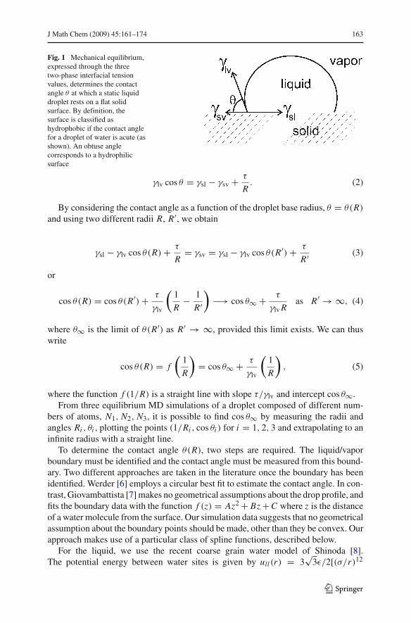
The contact angle of a static droplet of liquid on a flat solid surface represents a state ofmechanical equilibrium, and as such is determined by a balance between three interfa-cial tensions: the liquid/vapor surface tension, !lv, the solid/vapor surface tension, !sv,and the solid/liquid interfacial tension, !sl (see Fig. 1). Each pair of phases meets on atwo-manifold called an interface, and all three phases meet on a one-manifold calledthe three-phase line. For each point on the three-phase line there are three vectors,one for each interface, that act perpendicularly to the three-phase line and tangentiallyto their corresponding interface. The equilibrium relation between these vectors isknown as Young’s equation, where " is the Young contact angle.1

!lv cos " = !sl " !sv. (1)

However, Young’s equation is only valid for macroscopic droplets. For microscopicdroplets, the contact angle is influenced by the three-phase solid/liquid/vapor contactline, which contributes an additional energy per unit length called the line tension #

[5]. The modified Young’s equation accounts for the effect of line tension, where R isthe radius of the base of the droplet (in contact with the solid).

1 Note that some authors define the Young contact angle as ($ " " ), which changes the Young equation ina trivial manner.

123

J Math Chem (2009) 45:161–174 163

Fig. 1 Mechanical equilibrium,expressed through the threetwo-phase interfacial tensionvalues, determines the contactangle " at which a static liquiddroplet rests on a flat solidsurface. By definition, thesurface is classified ashydrophobic if the contact anglefor a droplet of water is acute (asshown). An obtuse anglecorresponds to a hydrophilicsurface

!lv cos " = !sl " !sv + #

R. (2)

By considering the contact angle as a function of the droplet base radius, " = "(R)

and using two different radii R, R#, we obtain

!sl " !lv cos "(R) + #

R= !sv = !sl " !lv cos "(R#) + #

R# (3)

or

cos "(R) = cos "(R#) + #

!lv

!1R

" 1R#

""$ cos "% + #

!lv Ras R# $ %, (4)

where "% is the limit of "(R#) as R# $ %, provided this limit exists. We can thuswrite

cos "(R) = f!

1R

"= cos "% + #

!lv

!1R

", (5)

where the function f (1/R) is a straight line with slope #/!lv and intercept cos "%.From three equilibrium MD simulations of a droplet composed of different num-

bers of atoms, N1, N2, N3, it is possible to find cos "% by measuring the radii andangles Ri , "i , plotting the points (1/Ri , cos "i ) for i = 1, 2, 3 and extrapolating to aninfinite radius with a straight line.

To determine the contact angle "(R), two steps are required. The liquid/vaporboundary must be identified and the contact angle must be measured from this bound-ary. Two different approaches are taken in the literature once the boundary has beenidentified. Werder [6] employs a circular best fit to estimate the contact angle. In con-trast, Giovambattista [7] makes no geometrical assumptions about the drop profile, andfits the boundary data with the function f (z) = Az2 + Bz + C where z is the distanceof a water molecule from the surface. Our simulation data suggests that no geometricalassumption about the boundary points should be made, other than they be convex. Ourapproach makes use of a particular class of spline functions, described below.

For the liquid, we use the recent coarse grain water model of Shinoda [8].The potential energy between water sites is given by ull(r) = 3

&3%/2[(&/r)12

123

164 J Math Chem (2009) 45:161–174

"(&/r)4], where r is the distance between the sites, and where % = 0.895 kcal/mol,& = 0.437 nm. We choose N1 = 11, 000, N2 = 22, 000, and N3 = 44, 000 for thenumber of water sites in a liquid droplet. The potential energy between an infinitelyextended flat solid and a liquid particle is given by [9] Usl(d) = a%& 9d"6 "b%& 6d"3,with a = 0.0338, b = 0.118, and & = 0.4 nm. The value of % determines whether,and to what extent, the solid object is hydrophobic or hydrophilic. d is the distancebetween the liquid particle and the solid. The droplet base radius Ri and contact angle"i = "(Ri ) are measured from a room temperature MD simulation as follows: afterthe droplet has equilibrated from an initial hemispherical geometry where the solidoccupies the region z ' 0 (1 ns), the spatial coordinates of all the liquid atoms aresaved every 40 ps. To determine Ri , we choose a small % > 0 and project the liquidparticles in the region 0 < z < % onto the plane z = 0 for each set of coordinates,giving a diffuse circle. We then identify the boundary of this circle, which is the three-phase contact line, by applying the following algorithm: every point on the boundaryhas the special property that there is a line passing through it which divides the planez = 0 into two regions: a region containing all the other points, and an empty region.We note that this boundary algorithm is valid for convex sets only, and that in practiceone must allow a few points in the “empty” region due to thermal fluctuations.

For a circle of radius R centered at the origin, the distance to a point (x j , y j )

on the circular boundary identified above is |(x2j + y2

j )1/2 " R|. In order to find

the radius which best fits these points, we need to minimize the function f (R) =#Nj=1((x2

j + y2j )

1/2 " R)2 where N is the number of points on the boundary. The

minimum is R = #Nj=1(x2

j + y2j )

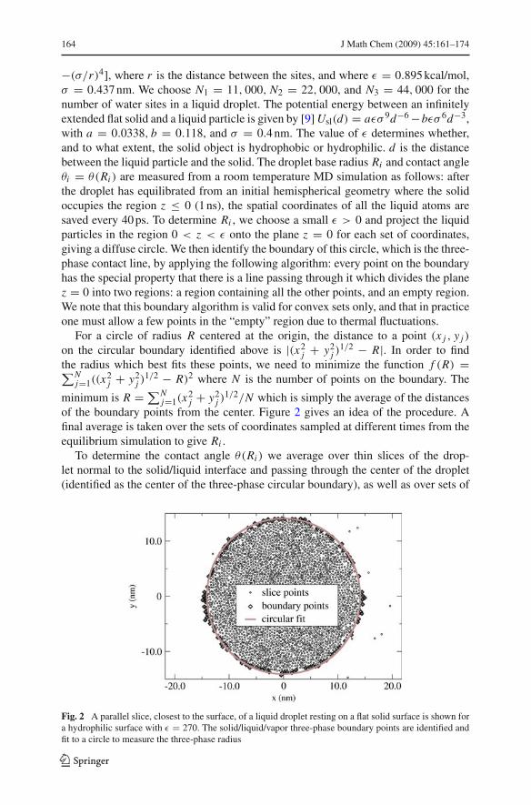
1/2/N which is simply the average of the distancesof the boundary points from the center. Figure 2 gives an idea of the procedure. Afinal average is taken over the sets of coordinates sampled at different times from theequilibrium simulation to give Ri .

To determine the contact angle "(Ri ) we average over thin slices of the drop-let normal to the solid/liquid interface and passing through the center of the droplet(identified as the center of the three-phase circular boundary), as well as over sets of

Fig. 2 A parallel slice, closest to the surface, of a liquid droplet resting on a flat solid surface is shown fora hydrophilic surface with % = 270. The solid/liquid/vapor three-phase boundary points are identified andfit to a circle to measure the three-phase radius

123

J Math Chem (2009) 45:161–174 165

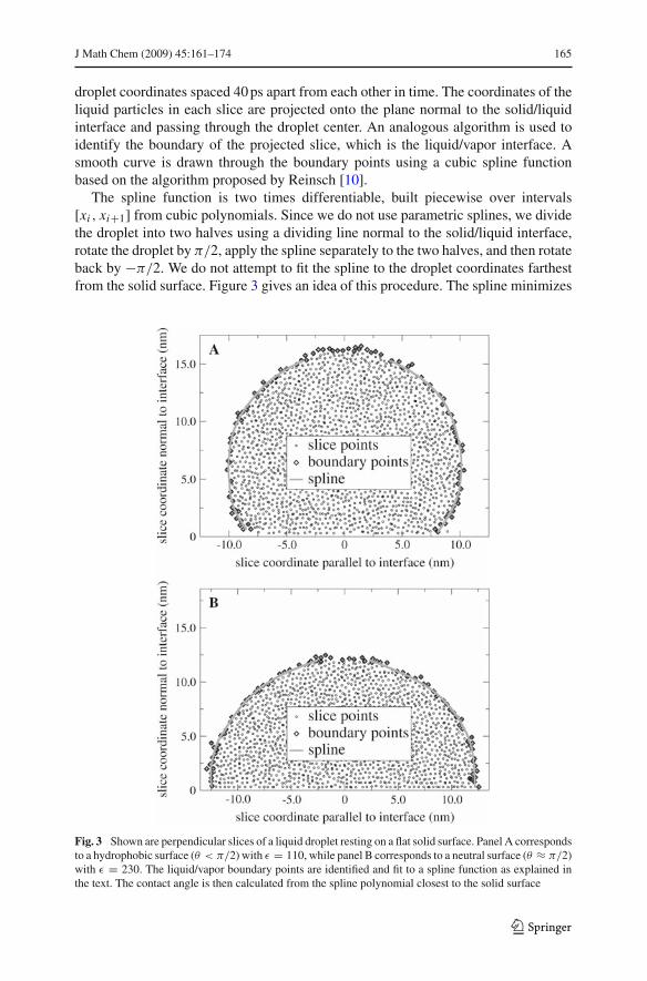
droplet coordinates spaced 40 ps apart from each other in time. The coordinates of theliquid particles in each slice are projected onto the plane normal to the solid/liquidinterface and passing through the droplet center. An analogous algorithm is used toidentify the boundary of the projected slice, which is the liquid/vapor interface. Asmooth curve is drawn through the boundary points using a cubic spline functionbased on the algorithm proposed by Reinsch [10].

The spline function is two times differentiable, built piecewise over intervals[xi , xi+1] from cubic polynomials. Since we do not use parametric splines, we dividethe droplet into two halves using a dividing line normal to the solid/liquid interface,rotate the droplet by $/2, apply the spline separately to the two halves, and then rotateback by "$/2. We do not attempt to fit the spline to the droplet coordinates farthestfrom the solid surface. Figure 3 gives an idea of this procedure. The spline minimizes

Fig. 3 Shown are perpendicular slices of a liquid droplet resting on a flat solid surface. Panel A correspondsto a hydrophobic surface (" < $/2) with % = 110, while panel B corresponds to a neutral surface (" ( $/2)with % = 230. The liquid/vapor boundary points are identified and fit to a spline function as explained inthe text. The contact angle is then calculated from the spline polynomial closest to the solid surface

123

166 J Math Chem (2009) 45:161–174

$ xn

x0

g##(x)2 dx (6)

among all functions g(x) such that

n%

i=0

!g(xi ) " yi

'yi

"2

' S, g ) C2[x0, xn], (7)

where 'yi and S are parameters that control the smoothness of the curve. We takeS = N " (2N )1/2 where N is the number of points that the spline is approximat-ing (the number of boundary points in the left or right hand side of one slice). This isconsistent with the value range recommended by Reinsch [10], namely N "(2N )1/2 'S ' N + (2N )1/2.

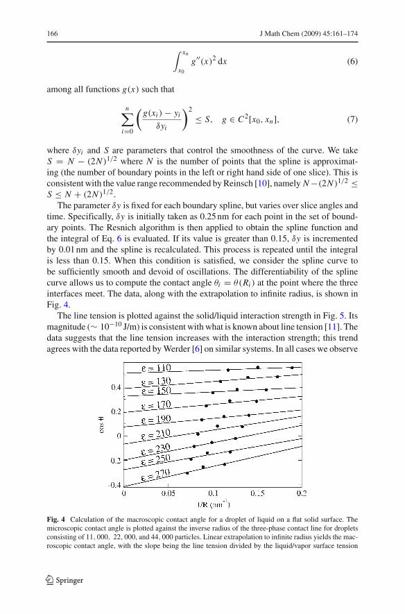
The parameter 'y is fixed for each boundary spline, but varies over slice angles andtime. Specifically, 'y is initially taken as 0.25 nm for each point in the set of bound-ary points. The Resnich algorithm is then applied to obtain the spline function andthe integral of Eq. 6 is evaluated. If its value is greater than 0.15, 'y is incrementedby 0.01 nm and the spline is recalculated. This process is repeated until the integralis less than 0.15. When this condition is satisfied, we consider the spline curve tobe sufficiently smooth and devoid of oscillations. The differentiability of the splinecurve allows us to compute the contact angle "i = "(Ri ) at the point where the threeinterfaces meet. The data, along with the extrapolation to infinite radius, is shown inFig. 4.

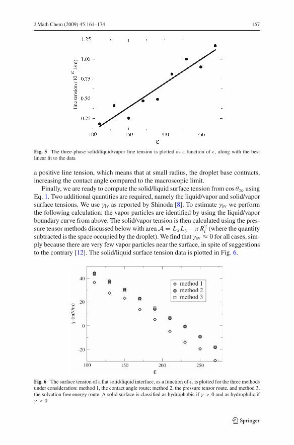
The line tension is plotted against the solid/liquid interaction strength in Fig. 5. Itsmagnitude (! 10"10 J/m) is consistent with what is known about line tension [11]. Thedata suggests that the line tension increases with the interaction strength; this trendagrees with the data reported by Werder [6] on similar systems. In all cases we observe

Fig. 4 Calculation of the macroscopic contact angle for a droplet of liquid on a flat solid surface. Themicroscopic contact angle is plotted against the inverse radius of the three-phase contact line for dropletsconsisting of 11, 000, 22, 000, and 44, 000 particles. Linear extrapolation to infinite radius yields the mac-roscopic contact angle, with the slope being the line tension divided by the liquid/vapor surface tension

123

J Math Chem (2009) 45:161–174 167

Fig. 5 The three-phase solid/liquid/vapor line tension is plotted as a function of %, along with the bestlinear fit to the data

a positive line tension, which means that at small radius, the droplet base contracts,increasing the contact angle compared to the macroscopic limit.

Finally, we are ready to compute the solid/liquid surface tension from cos "% usingEq. 1. Two additional quantities are required, namely the liquid/vapor and solid/vaporsurface tensions. We use !lv as reported by Shinoda [8]. To estimate !sv we performthe following calculation: the vapor particles are identified by using the liquid/vaporboundary curve from above. The solid/vapor tension is then calculated using the pres-sure tensor methods discussed below with area A = Lx L y "$ R2

i (where the quantitysubtracted is the space occupied by the droplet). We find that !sv ( 0 for all cases, sim-ply because there are very few vapor particles near the surface, in spite of suggestionsto the contrary [12]. The solid/liquid surface tension data is plotted in Fig. 6.

Fig. 6 The surface tension of a flat solid/liquid interface, as a function of %, is plotted for the three methodsunder consideration: method 1, the contact angle route; method 2, the pressure tensor route, and method 3,the solvation free energy route. A solid surface is classified as hydrophobic if ! > 0 and as hydrophilic if! < 0

123

168 J Math Chem (2009) 45:161–174

3 Method 2: pressure tensor

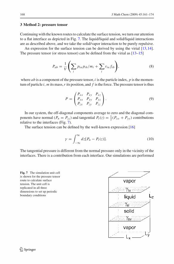
Continuing with the known routes to calculate the surface tension, we turn our attentionto a flat interface as depicted in Fig. 7. The liquid/liquid and solid/liquid interactionsare as described above, and we take the solid/vapor interaction to be purely repulsive.

An expression for the surface tension can be derived by using the virial [13,14].The pressure tensor (or stress tensor) can be defined from the virial as [13–15]

Pab = 1V

&%

i

pia pib/mi +%

i

ria fib

'

, (8)

where ab is a component of the pressure tensor, i is the particle index, p is the momen-tum of particle i, m its mass, r its position, and f is the force. The pressure tensor is thus

P =

(

)Pxx Pxy PxzPyx Pyy PyzPzx Pzy Pzz

*

+ . (9)

In our system, the off-diagonal components average to zero and the diagonal com-ponents have normal (Pn = Pzz) and tangential Pt (z) = 1

2 (Pxx + Pyy) contributionsrelative to the interfaces (Fig. 7).

The surface tension can be defined by the well-known expression [16]

! =$ %

"%dz[Pn " Pt (z)]. (10)

The tangential pressure is different from the normal pressure only in the vicinity of theinterfaces. There is a contribution from each interface. Our simulations are performed

Fig. 7 The simulation unit cellis shown for the pressure tensorroute to calculate surfacetension. The unit cell isreplicated in all threedimensions to set up periodicboundary conditions

123

J Math Chem (2009) 45:161–174 169

in an orthorhombic box as depicted in Fig. 7 with sides Lx , L y, Lz , where the area ofthe interface is A = Lx L y . The total surface tension can be rewritten as

! = Lz(Pn " P̄t ), (11)

where P̄t is the average tangential pressure Pt (z). Note that the box size dependenceof Eq. 11 is 1/A since V = Lx L y Lz .

We can divide the total surface tension into contributions from the individual surfacetensions as [17]

! = !sl + !lv + !sv. (12)

This is possible because the interfaces are separated from each other and do not inter-act—i.e., there is a bulk phase region between each interface. From previous work,we have !lv = 71 mN/m [8]. Also, !sv ( 0, because the surface is constructed to bepurely repulsive on the vapor side.

Thus we can determine !sl as

!sl = *Pn " Pt + " !lv. (13)

The resulting solid/liquid surface tension data is plotted in Fig. 6.

4 Method 3: solvation free energy

In this section we introduce a new method to calculate solid/liquid surface tension,based on the thermodynamic definition of surface tension, ! , given by [18]

! ,!

(G(A

"

N ,P,T, (14)

where G is the Gibbs free energy and A is the interfacial area.Motivated by this definition, we will compute the solvation free energy of a spher-

ical solid of radius R and recover the flat result by taking the limit as R $ %. Inorder to do this, we must adapt the flat potential Usl(d) = a%& 9d"6 " b%& 6d"3 to acurved solid geometry. This is straightforward, and is done as follows [19].

Suppose that an individual atomic crystal lattice site in the solid interacts with aparticle in the liquid via a distance-dependent potential energy u(r). Approximatingthe solid as a continuum with number density ) = N/V that occupies the semi-infiniteregion z ' 0, a liquid particle at height z > 0 interacts with the entire solid object as

U (z) =$ %

zdr

$ 2$

0d"

$ $

$"cos"1(z/r)d* r2 sin * )u(r)

= 2$)

$ %

zru(r)[r " z]dr. (15)

123

170 J Math Chem (2009) 45:161–174

Two derivatives yield

u(+) = U ##(+)

2$)+. (16)

Using expressions (16) and Usl(d) = a%& 9d"6 " b%& 6d"3, we obtain

usl(r) = 21a%& 9

$)r"9 " 6b%& 6

$)r"6 (17)

as the potential energy between a particle in the liquid and a particle in the solid. Now,we once again approximate the solid as a continuum with number density ) = N/V ,but this time as a sphere of radius R. A liquid particle interacts with the entire solidsphere as

U (d, R) =$ R

0dr

$ 2$

0d"

$ $

0d*)r2 sin *u([r2+(d + R)2 " 2r cos *(d + R)]1/2)

= 4a%& 9 R3

5d6

35d4 + 140Rd3 + 252R2d2 + 224R3d + 80R4

(d + R)(d + 2R)6

" 8b%& 6 R3

d3(d + 2R)3 , (18)

where d is the distance between the liquid particle and the solid.We now change variables from U (d, R) to U (r, R) where r = d + R, the distance

between the centers of mass of the solid sphere and the liquid particle. Let us now con-sider the significance of the two partial derivatives (U/(r and (U/( R. First, "(U/(r(the gradient of the potential) gives the force that acts between the two particles ontheir respective centers of mass. This is the force used to move the particles during amolecular dynamics simulation. Second,

#i "(U/( R, summed over all liquid par-

ticles i , represents the force acting on the sphere radius. However, the sphere radiusis fixed and hence does not experience this force. Conceptually, to balance this forceso that the sphere radius experiences a net force of zero, we should apply an externalforce to the sphere radius of

#i (U/( R at each step of the simulation. However, we

do not actually apply this external force since the sphere radius is in no danger ofchanging. Nonetheless, we may calculate the required external restoring force on thesphere radius, known as the force of constraint, and record its value during a computersimulation. Its average value over an equilibrium simulation is called the mean forceof constraint; let us denote it by PMF(R). By performing separation simulations withspheres of different radii, we can integrate PMF(R) starting from R = 0 to obtainthe solvation free energy G(R). G(R) can be thought of as the free energy cost of“growing” the sphere into water. It can also be thought of as the free energy cost oftransferring a spherical solid of radius R from an ideal gas reference state to a liquid.We have verified the validity of the PMF route to G(R) by performing free energycalculations corresponding to the later interpretation, where a radius R sphere is pulled

123

J Math Chem (2009) 45:161–174 171

from the vapor phase, through the liquid/vapor interface, and into the liquid phase ina simulation system of an infinitely extended, thick, slab of liquid.

From the definition of surface tension in Eq. 14, we have

limR$%

G(R)

4$ R2 = ! . (19)

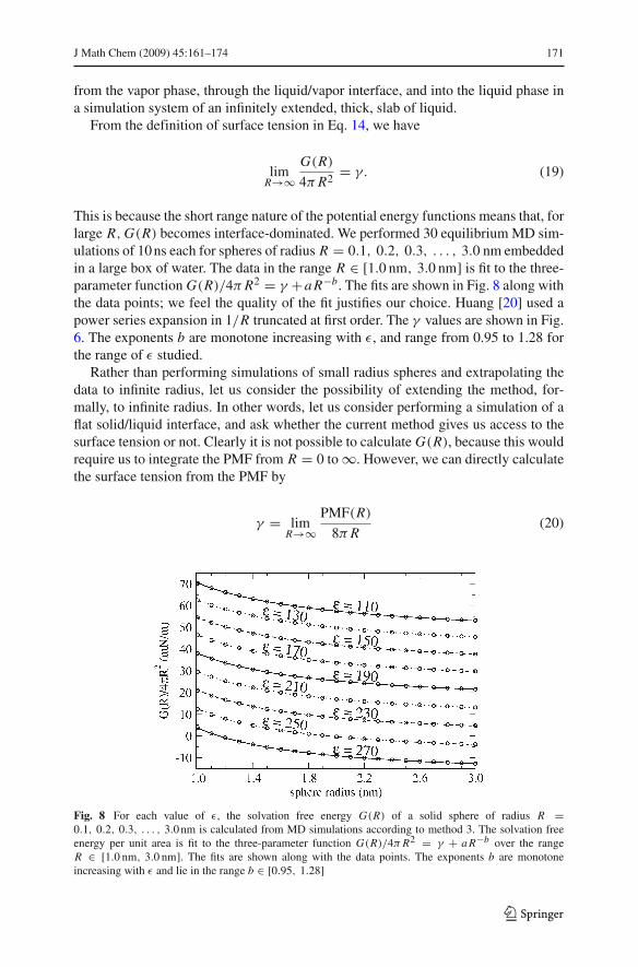
This is because the short range nature of the potential energy functions means that, forlarge R, G(R) becomes interface-dominated. We performed 30 equilibrium MD sim-ulations of 10 ns each for spheres of radius R = 0.1, 0.2, 0.3, . . . , 3.0 nm embeddedin a large box of water. The data in the range R ) [1.0 nm, 3.0 nm] is fit to the three-parameter function G(R)/4$ R2 = ! +a R"b. The fits are shown in Fig. 8 along withthe data points; we feel the quality of the fit justifies our choice. Huang [20] used apower series expansion in 1/R truncated at first order. The ! values are shown in Fig.6. The exponents b are monotone increasing with %, and range from 0.95 to 1.28 forthe range of % studied.

Rather than performing simulations of small radius spheres and extrapolating thedata to infinite radius, let us consider the possibility of extending the method, for-mally, to infinite radius. In other words, let us consider performing a simulation of aflat solid/liquid interface, and ask whether the current method gives us access to thesurface tension or not. Clearly it is not possible to calculate G(R), because this wouldrequire us to integrate the PMF from R = 0 to %. However, we can directly calculatethe surface tension from the PMF by

! = limR$%

PMF(R)

8$ R(20)

Fig. 8 For each value of %, the solvation free energy G(R) of a solid sphere of radius R =0.1, 0.2, 0.3, . . . , 3.0 nm is calculated from MD simulations according to method 3. The solvation freeenergy per unit area is fit to the three-parameter function G(R)/4$ R2 = ! + a R"b over the rangeR ) [1.0 nm, 3.0 nm]. The fits are shown along with the data points. The exponents b are monotoneincreasing with % and lie in the range b ) [0.95, 1.28]

123

172 J Math Chem (2009) 45:161–174

for the following reason: writing G(R)/4$ R2 = ! + h(R), where h(R) $ 0 asR $ %, we have PMF(R)/8$ R = ! + h(R) + Rh#(R)/2 since PMF is the deriv-ative of G(R). Equation 20 is valid if Rh#(R)/2 $ 0 as R $ %, which holds sincewe estimated numerically that h(R) = a R"b with b ) (0.95, 1.28).

The limiting expressions for the potential energy and its derivatives are also well-defined: for example it is straightforward to verify that Eq. 18 reduces to Usl(d) =a%& 9d"6 "b%& 6d"3, limR$% U (d, R) = Usl(d). Unfortunately, there are two prob-lems blocking the use of the sphere method for flat interfaces. The first problem is thescaling of PMF(R) with R, and the second problem arises from the use of periodicboundary conditions in computer simulations. We will now discuss these problems indetail.

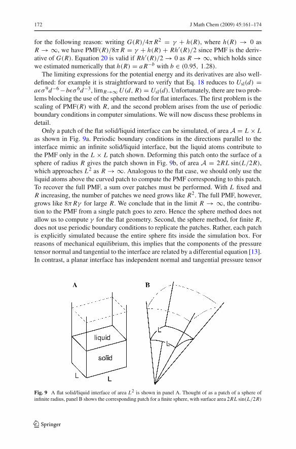
Only a patch of the flat solid/liquid interface can be simulated, of area A = L - Las shown in Fig. 9a. Periodic boundary conditions in the directions parallel to theinterface mimic an infinite solid/liquid interface, but the liquid atoms contribute tothe PMF only in the L - L patch shown. Deforming this patch onto the surface of asphere of radius R gives the patch shown in Fig. 9b, of area A = 2RL sin(L/2R),which approaches L2 as R $ %. Analogous to the flat case, we should only use theliquid atoms above the curved patch to compute the PMF corresponding to this patch.To recover the full PMF, a sum over patches must be performed. With L fixed andR increasing, the number of patches we need grows like R2. The full PMF, however,grows like 8$ R! for large R. We conclude that in the limit R $ %, the contribu-tion to the PMF from a single patch goes to zero. Hence the sphere method does notallow us to compute ! for the flat geometry. Second, the sphere method, for finite R,does not use periodic boundary conditions to replicate the patches. Rather, each patchis explicitly simulated because the entire sphere fits inside the simulation box. Forreasons of mechanical equilibrium, this implies that the components of the pressuretensor normal and tangential to the interface are related by a differential equation [13].In contrast, a planar interface has independent normal and tangential pressure tensor

Fig. 9 A flat solid/liquid interface of area L2 is shown in panel A. Thought of as a patch of a sphere ofinfinite radius, panel B shows the corresponding patch for a finite sphere, with surface area 2RL sin(L/2R)

123

J Math Chem (2009) 45:161–174 173

values, which is why they both appear explicitly in Eq. 11; the sphere method lacksany explicit contributions from tangential forces.

5 Conclusions

We have presented three topologically different methods for computing the surfacetension between a liquid and a flat solid. In method 1, a hemispherical droplet of liquidsurrounded by vapor rests on a flat solid surface. The surface tension is obtained bymeasuring the angle at which the liquid/vapor boundary meets the solid surface. Theline tension associated with the three-phase boundary is calculated and is shown to beproportional to the strength of the solid/liquid interaction. In method 2, all three phasesare also present, but only meet in pairs at planar interfaces. The pressure tensor is usedto compute the surface tension. In method 3, a spherical solid is surrounded by liquid,and the vapor phase is absent. The solvation free energy of the solid, which is usedto obtain the surface tension, is calculated by a novel method based on constrainedmolecular dynamics. Although method 2 is the most efficient because no extrapolationis required, it also gives the least amount of information. Method 1 allows the linetension to be computed, which is crucial to understanding the behavior of nanoscalesystems with three-phase boundaries. Method 3 gives access to spherical solids, open-ing the door to colloid science. Methods 2 and 3 are in perfect agreement, whereasmethod 1 systematically underestimates the surface tension as a function of the hydro-phobicity/hydrophilicity of the surface (see Fig. 6). We do not understand why thisdiscrepancy exists. We will continue to work on this problem.

Acknowledgements The authors acknowledge the Donors of the American Chemical Society PetroleumResearch Fund for partial support of this research. Dr. Moore would like to acknowledge that this researchwas supported in part by a gift from the H.O. West Foundation, a grant from the University of the Sci-ences in Philadelphia (USP), a grant from the National Institute of Health (1R15GM075990-01), and grantsfrom the National Science Foundation (CHE-0420556 and CCF-0622162). The authors would also liketo acknowledge the Texas Advanced Computing Center (TACC) at The University of Texas at Austin forproviding HPC resources that have contributed to the research results reported within this paper.

References

1. Y. Lin, H. Skaff, T. Emrick, A.D. Dinsmore, T.P. Russell, Science 299, 226–229 (2003)2. D. Wang, H. Duan, H. Möhwald, Soft Matter 1, 412–416 (2005)3. B.P. Binks, J.H. Clint, Languir 18, 1270–1273 (2002)4. E. Salomons, M. Mareschal, J. Phys. Condens. Matter 3, 3645–3661 (1991)5. J.Y. Wang, S. Betelu, B.M. Law, Phys. Rev. E 63, 031601 (2001)6. T. Werder, J.H. Walther, R.L. Jaffe, T. Halicioglu, P. Koumoutsakos, J. Phys. Chem. B 107, 1345–1352

(2003)7. N. Giovambattista, P.G. Debenedetti, P.J. Rossky, J. Phys. Chem. B 111, 9581–9587 (2007)8. W. Shinoda, R. Devane, M.L. Klein, Mol. Simul. 33, 27–36 (2007)9. S.O. Nielsen, G. Srinivas, M.L. Klein, J. Chem. Phys. 123, 124907 (2005)

10. C.H. Reinsch, Numer. Math. 10, 177–183 (1967); 16, 451–454 (1971)11. J. Drelich, Colloids Surf. A 116, 43–54 (1996)12. S.M. Dammer, D. Lohse, Phys. Rev. Lett. 96, 206101 (2006)13. M.P. Allen, D.J. Tildesley, Computer Simulations of Liquids (Oxford University Press, Oxford, 1987)14. J.H. Irving, J.G. Kirkwood, J. Chem. Phys. 18, 817–829 (1950)

123

174 J Math Chem (2009) 45:161–174

15. Y. Zhang, S.E. Feller, B.R. Brooks, R.W. Pastor, J. Chem. Phys. 103, 10252–10266 (1995)16. T.L. Hill, Statistical Thermodynamics (Addison-Wesley, Reading, MA 1962)17. S.E. Feller, Y. Zhang, R.W. Pastor, J. Chem. Phys. 103, 10267–10276 (1995)18. W.J. Moore, Physical Chemistry, 4th edn. (Prentice-Hall, New Jersey, 1972)19. S.O. Nielsen, G. Srinivas, C.F. Lopez, M.L. Klein, Phys. Rev. Lett. 94, 228301 (2005)20. D.M. Huang, P.L. Geissler, D. Chandler, J. Phys. Chem. B 105, 6704–6709 (2001)

123