Calculation of Invariant Manifold for

Isothermal Spatially Homogeneous

Reactions with Detailed Kinetics

By: Clayton R. Swope

For: Drs. Joseph M. Powers, Samuel Paolucci

AME 499: Undergraduate Research

Department of Aerospace and Mechanical Engineering

University of Notre Dame

Notre Dame, IN 46556

August 2003

2

Abstract

The objective of this research was to determine the concentrations of the

intermediate molecular species with respect to time during the isothermal spatially

homogeneous decomposition of ozone in order to identify the invariant manifold for

the system. The fourteen elementary reactions of the decomposition process were

identified, and the reaction rates of each constituent intermediate species were

formulated from these reactions. The steady-state equilibrium conditions and an

additional six non-physical critical points were determined and locally classified

using eigensystem analysis. The reaction rate equations were numerically solved to

produce the system response so as to predict the concentrations of the intermediate

species as a function of time. The one-dimensional manifold that stretched from the

stable physical steady-state equilibrium to a non-physical unstable source was

identified and analyzed. The resulting analysis yielded a description of the physical

reaction process for specific physical initial concentrations of the constituent

elements as the elements approached the one-dimensional manifold and steady-

state conditions.

3

1 Introduction

1.1 Combustion

The chemical processes involved in the combustion process is the focus of much

study; for without a complete understanding of how the major species involved in

oxidation interact over time, it is difficult to accurately model an event. The

simplicity of the stoichiometric balance equations used to represent many high-

temperature combustion processes, such as the decomposition of ozone, is rather

deceptive in that this representation assumes the products of such a reaction are

solely mixtures of ideal products. True high-temperature combustion processes

usually produce numerous minor species – some in relatively large quantities – of

the associated chemical components as the major chemical species tend to dissociate.

An understanding of the equilibrium or steady-state of a chemical combustion

process requires an understanding of how the properties of a chemical system vary

with time and initial conditions.

The manner in which the amounts of the components involved in a combustion

process change over time is controlled and influenced by the chemical reaction rates

of the system under study. The study of these reactions and their associated

chemical reaction rates is referred to as chemical kinetics. The goal of chemical

kinetics is to define the specific pathways of a chemical system from initial reactants

to final equilibrium products and define their reactions rates along this path.

Numerical solutions that take into account the chemistry of a system are generally

required to solve for these rates and generate the corresponding reaction response.

4

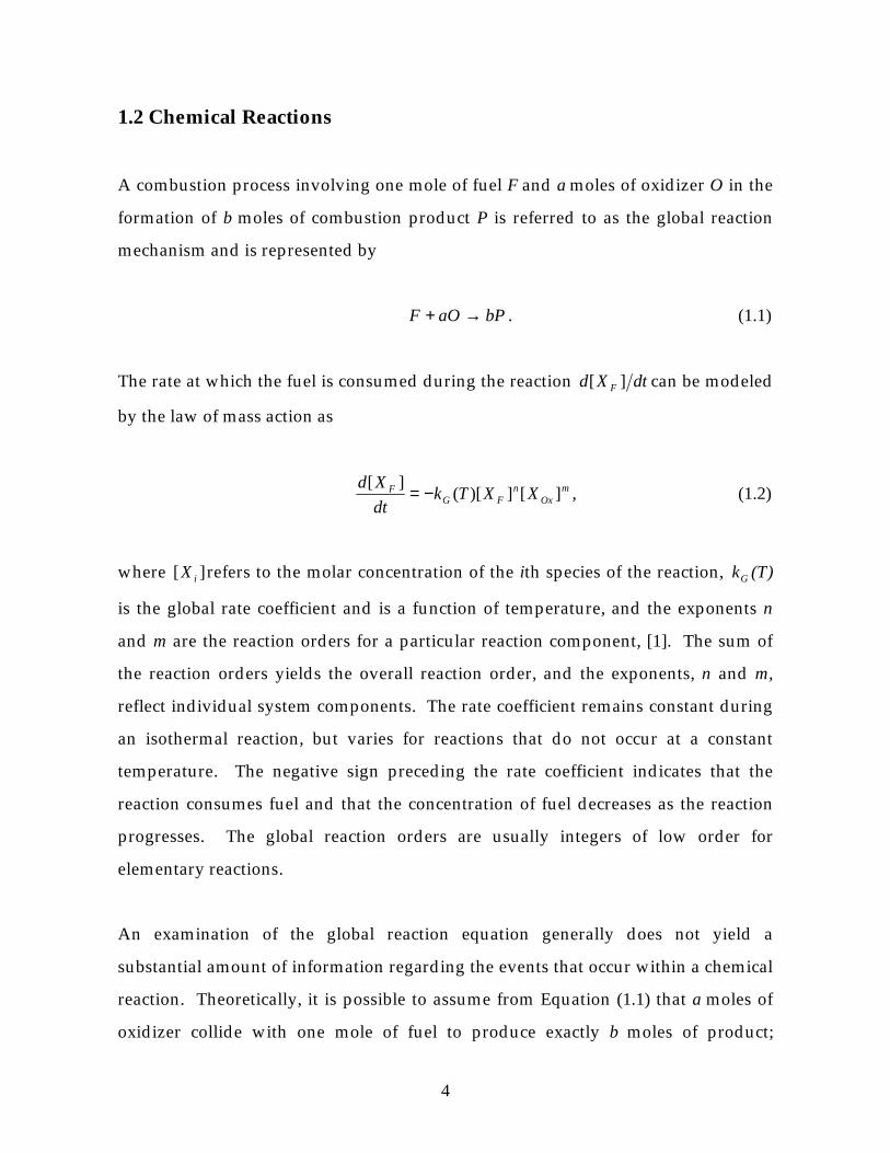
1.2 Chemical Reactions

A combustion process involving one mole of fuel F and a moles of oxidizer O in the

formation of b moles of combustion product P is referred to as the global reaction

mechanism and is represented by

bPaOF →+ . (1.1)

The rate at which the fuel is consumed during the reaction dtXd F ][ can be modeled

by the law of mass action as

mOx

nFG

F XXTkdt

Xd][])[(

][−= , (1.2)

where ][ iX refers to the molar concentration of the ith species of the reaction, Gk (T)

is the global rate coefficient and is a function of temperature, and the exponents n

and m are the reaction orders for a particular reaction component, [1]. The sum of

the reaction orders yields the overall reaction order, and the exponents, n and m,

reflect individual system components. The rate coefficient remains constant during

an isothermal reaction, but varies for reactions that do not occur at a constant

temperature. The negative sign preceding the rate coefficient indicates that the

reaction consumes fuel and that the concentration of fuel decreases as the reaction

progresses. The global reaction orders are usually integers of low order for

elementary reactions.

An examination of the global reaction equation generally does not yield a

substantial amount of information regarding the events that occur within a chemical

reaction. Theoretically, it is possible to assume from Equation (1.1) that a moles of

oxidizer collide with one mole of fuel to produce exactly b moles of product;

5

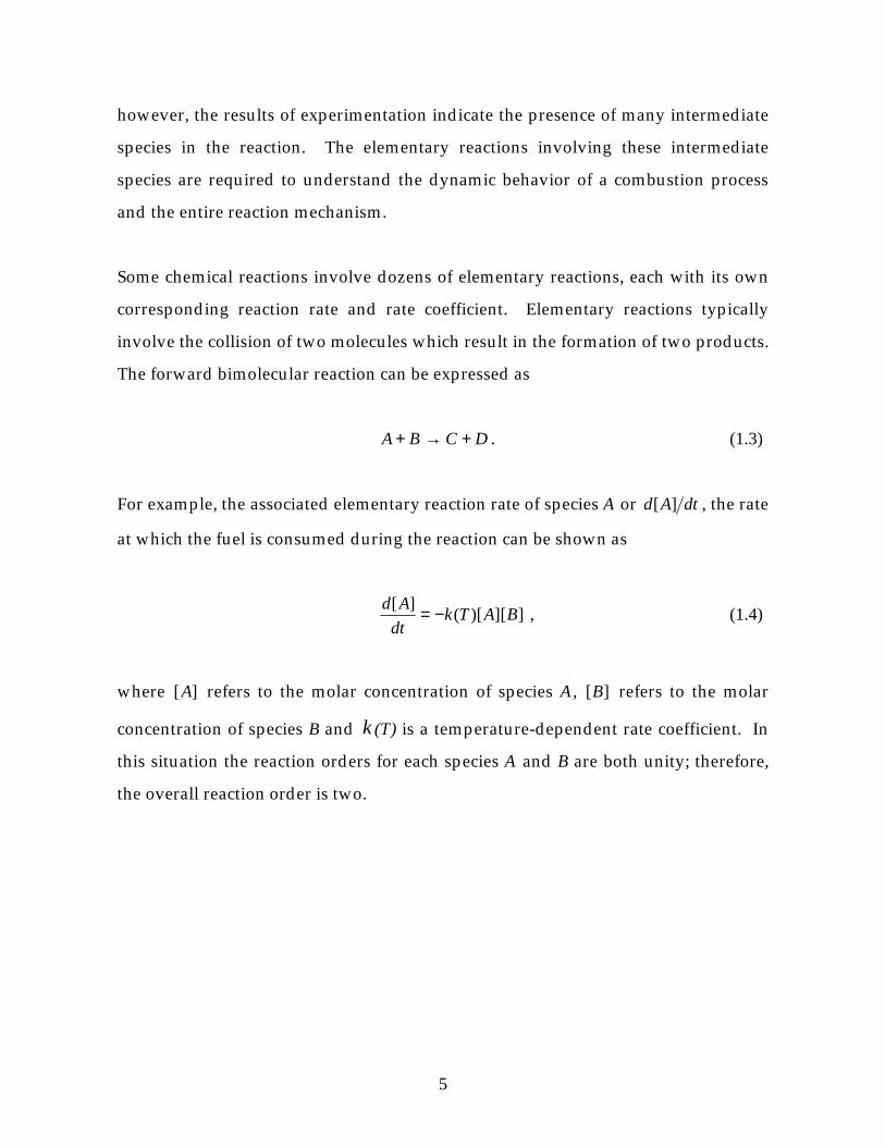
however, the results of experimentation indicate the presence of many intermediate

species in the reaction. The elementary reactions involving these intermediate

species are required to understand the dynamic behavior of a combustion process

and the entire reaction mechanism.

Some chemical reactions involve dozens of elementary reactions, each with its own

corresponding reaction rate and rate coefficient. Elementary reactions typically

involve the collision of two molecules which result in the formation of two products.

The forward bimolecular reaction can be expressed as

DCBA +→+ . (1.3)

For example, the associated elementary reaction rate of species A or dtAd ][ , the rate

at which the fuel is consumed during the reaction can be shown as

]][)[(][

BATkdt

Ad −= , (1.4)

where ][A refers to the molar concentration of species A, ][B refers to the molar

concentration of species B and k (T) is a temperature-dependent rate coefficient. In

this situation the reaction orders for each species A and B are both unity; therefore,

the overall reaction order is two.

6

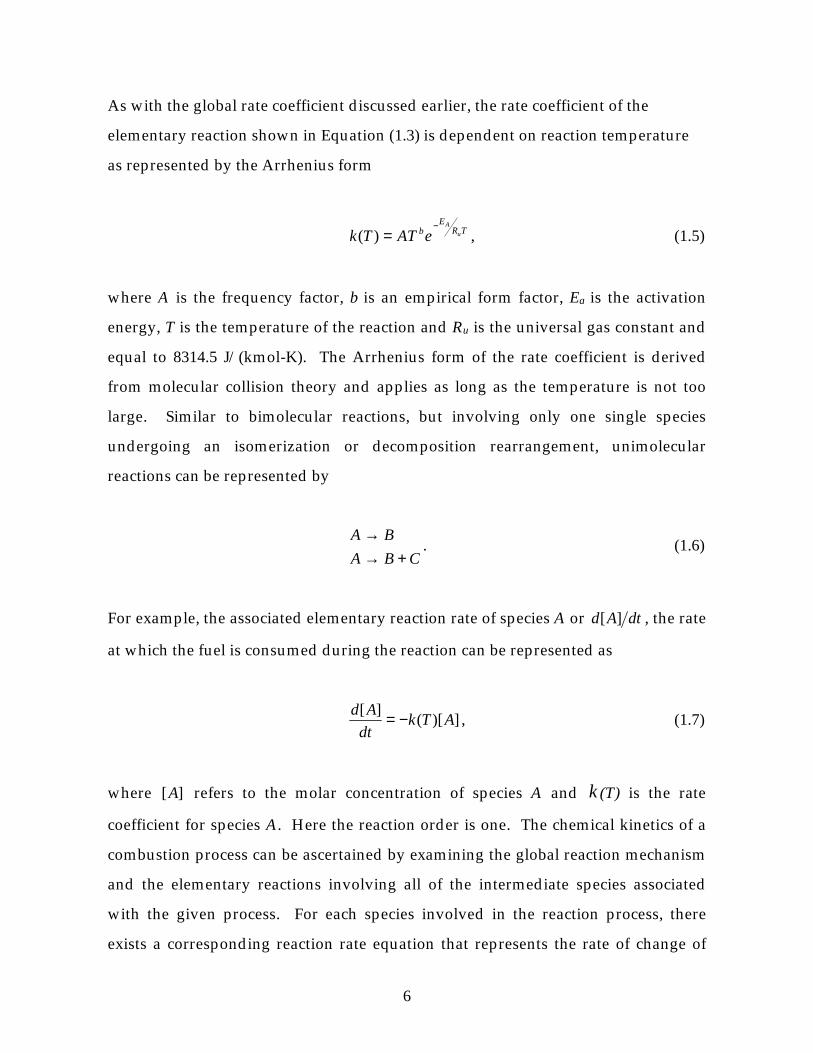
As with the global rate coefficient discussed earlier, the rate coefficient of the

elementary reaction shown in Equation (1.3) is dependent on reaction temperature

as represented by the Arrhenius form

TRE

b u

A

eATTk−

=)( , (1.5)

where A is the frequency factor, b is an empirical form factor, Ea is the activation

energy, T is the temperature of the reaction and Ru is the universal gas constant and

equal to 8314.5 J/(kmol-K). The Arrhenius form of the rate coefficient is derived

from molecular collision theory and applies as long as the temperature is not too

large. Similar to bimolecular reactions, but involving only one single species

undergoing an isomerization or decomposition rearrangement, unimolecular

reactions can be represented by

CBA

BA

+→→

. (1.6)

For example, the associated elementary reaction rate of species A or dtAd ][ , the rate

at which the fuel is consumed during the reaction can be represented as

])[(][

ATkdt

Ad −= , (1.7)

where ][A refers to the molar concentration of species A and k (T) is the rate

coefficient for species A. Here the reaction order is one. The chemical kinetics of a

combustion process can be ascertained by examining the global reaction mechanism

and the elementary reactions involving all of the intermediate species associated

with the given process. For each species involved in the reaction process, there

exists a corresponding reaction rate equation that represents the rate of change of

7

that particular species over time based directly on the elementary reactions involved

in the combustion process.

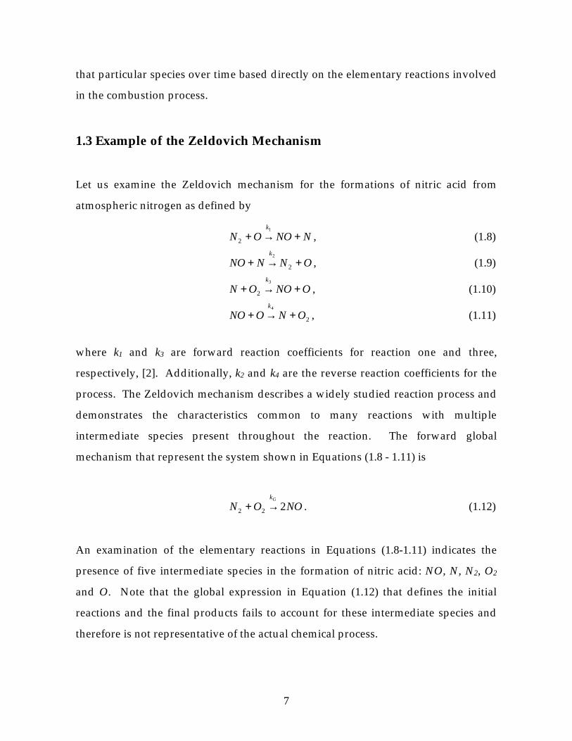
1.3 Example of the Zeldovich Mechanism

Let us examine the Zeldovich mechanism for the formations of nitric acid from

atmospheric nitrogen as defined by

NNOONk

+→+1

2 , (1.8)

ONNNOk

+→+ 2

2

, (1.9)

ONOONk

+→+3

2 , (1.10)

2

4

ONONOk

+→+ , (1.11)

where k1 and k3 are forward reaction coefficients for reaction one and three,

respectively, [2]. Additionally, k2 and k4 are the reverse reaction coefficients for the

process. The Zeldovich mechanism describes a widely studied reaction process and

demonstrates the characteristics common to many reactions with multiple

intermediate species present throughout the reaction. The forward global

mechanism that represent the system shown in Equations (1.8 - 1.11) is

NOONGk

222 →+ . (1.12)

An examination of the elementary reactions in Equations (1.8-1.11) indicates the

presence of five intermediate species in the formation of nitric acid: NO, N, N2, O2

and O. Note that the global expression in Equation (1.12) that defines the initial

reactions and the final products fails to account for these intermediate species and

therefore is not representative of the actual chemical process.

8

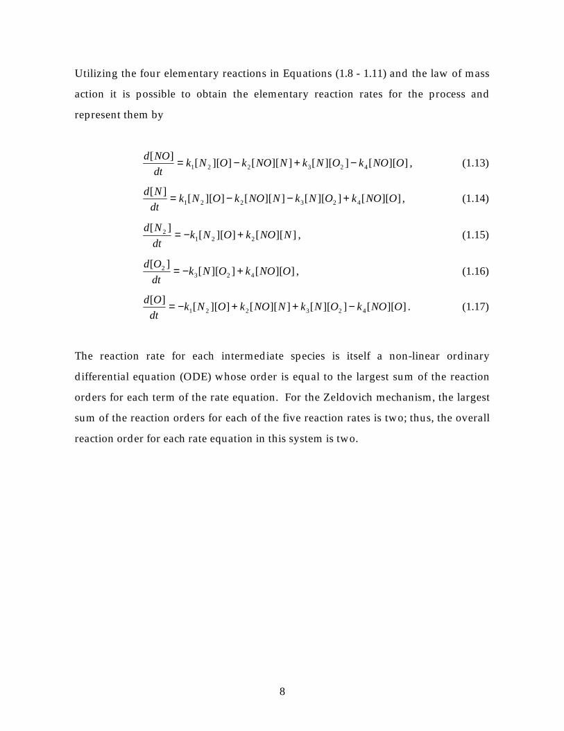
Utilizing the four elementary reactions in Equations (1.8 - 1.11) and the law of mass

action it is possible to obtain the elementary reaction rates for the process and

represent them by

]][[]][[]][[]][[][

423221 ONOkONkNNOkONkdt

NOd −+−= , (1.13)

]][[]][[]][[]][[][

423221 ONOkONkNNOkONkdt

Nd +−−= , (1.14)

]][[]][[][

2212 NNOkONk

dt

Nd +−= , (1.15)

]][[]][[][

4232 ONOkONk

dt

Od +−= , (1.16)

]][[]][[]][[]][[][

423221 ONOkONkNNOkONkdt

Od −++−= . (1.17)

The reaction rate for each intermediate species is itself a non-linear ordinary

differential equation (ODE) whose order is equal to the largest sum of the reaction

orders for each term of the rate equation. For the Zeldovich mechanism, the largest

sum of the reaction orders for each of the five reaction rates is two; thus, the overall

reaction order for each rate equation in this system is two.

9

2 Analysis Techniques

2.1 Ordinary Differential Equations

The evolution of species concentration during any reaction, like the Zeldovich

mechanism, is determined by a system of ODEs. Combustion processes can be

described by a system of ODEs representing the reaction rates of the intermediate

species derived from the elementary reaction equations and the law of mass action.

A complete solution for the ODEs will yield a description of the chemical kinetics of

system evolution over time. And as with the Zeldovich mechanism, the ODEs that

make up the representative system are usually stable and non-linear in nature. They

also typically lack explicit, closed form, solutions. In these situations, where no

closed form solution to the system is obtainable, it is necessary to compute

numerical solutions to the differential equations.

Numerical solutions to systems of ODEs cannot provide an exact closed functional

form to the given problem and instead produce a subset of points from the solution

space. These points contain numerical errors based upon the integration routine

used to perform the calculations; however, this error can be minimized by varying

several computational parameters, especially the length of the time steps used in the

integration and acceptable error tolerances of the routine. To obtain convergence

between the theoretical closed-form solution – and mimic the real-life behavior of a

chemical reaction – the distance between the individual points of the numerical

solution must be small enough to reflect all variations in the system at all times

scales of the reaction. Since these time-scales vary with time during any given

reaction, it is important to take into account the smallest to ensure an accurate

representation of the solution.

10

Stable systems approach a finite steady-state, while unstable systems approach

infinity as time progresses. Combustion processes begin at some initial state with

the initial reactants at some starting quantity and progress to steady-state over a

given time. The steady-state occurs as time approaches infinity as

combustion processes in closed systems can be shown to be stable. When no further

changes occur in the dependent variables of the system for continued changes of the

independent variables, the equilibrium state has been reached. For combustion

processes, the independent variable is time and the dependent variables are the

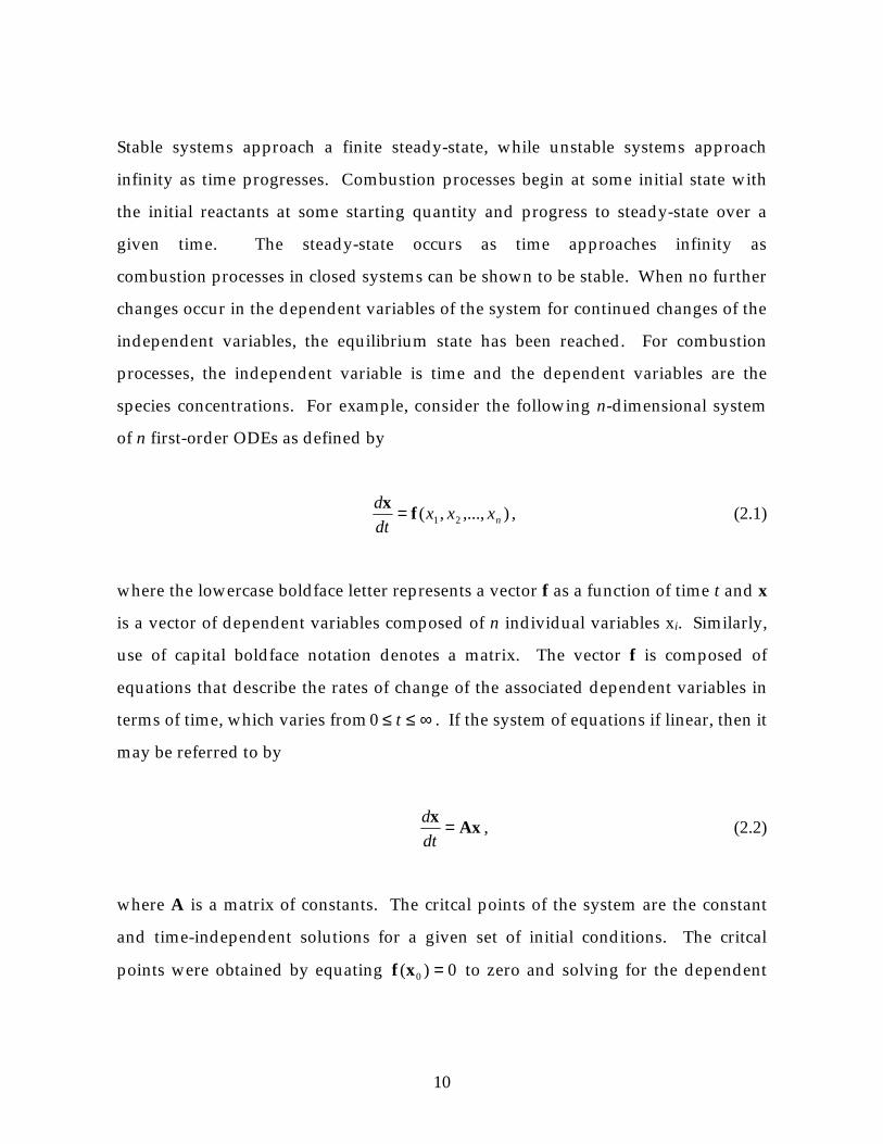
species concentrations. For example, consider the following n-dimensional system

of n first-order ODEs as defined by

),...,,( 21 nxxxdt

df

x = , (2.1)

where the lowercase boldface letter represents a vector f as a function of time t and x

is a vector of dependent variables composed of n individual variables xi. Similarly,

use of capital boldface notation denotes a matrix. The vector f is composed of

equations that describe the rates of change of the associated dependent variables in

terms of time, which varies from ∞≤≤ t0 . If the system of equations if linear, then it

may be referred to by

Axx =

dt

d, (2.2)

where A is a matrix of constants. The critcal points of the system are the constant

and time-independent solutions for a given set of initial conditions. The critcal

points were obtained by equating 0)( 0 =xf to zero and solving for the dependent

11

variables at this condition. And when 0)( 0 =xf , the rate of change is consequently

zero at critical point x0. The critical points may vary with intial conditions.

2.2 Eigenvalue and Eigenvector Analysis

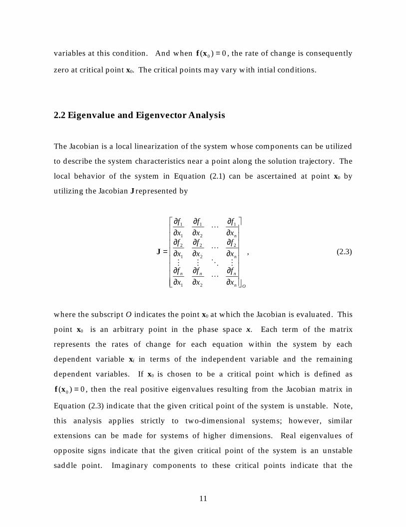
The Jacobian is a local linearization of the system whose components can be utilized

to describe the system characteristics near a point along the solution trajectory. The

local behavior of the system in Equation (2.1) can be ascertained at point x0 by

utilizing the Jacobian J represented by

On

nnn

n

n

x

f

x

f

x

f

x

f

x

f

x

fx

f

x

f

x

f

∂∂

∂∂

∂∂

∂∂

∂∂

∂∂

∂∂

∂∂

∂∂

=

L

MOMM

L

L

21

2

2

2

1

2

1

2

1

1

1

J , (2.3)

where the subscript O indicates the point x0 at which the Jacobian is evaluated. This

point x0 is an arbitrary point in the phase space x. Each term of the matrix

represents the rates of change for each equation within the system by each

dependent variable xi in terms of the independent variable and the remaining

dependent variables. If x0 is chosen to be a critical point which is defined as

0)( 0 =xf , then the real positive eigenvalues resulting from the Jacobian matrix in

Equation (2.3) indicate that the given critical point of the system is unstable. Note,

this analysis applies strictly to two-dimensional systems; however, similar

extensions can be made for systems of higher dimensions. Real eigenvalues of

opposite signs indicate that the given critical point of the system is an unstable

saddle point. Imaginary components to these critical points indicate that the

12

solution possesses an oscillatory component near the critical point with either a

stable or unstable spiral depending on the sign of the real part of the eigenvalues.

Real negative or positive eigenvalues indicate that the given point of the system is a

sink or source, respectively.

As mentioned before, the physical combustion processes modeled by a system of

ODEs are stable and thus approach some final equilibrium condition; however, the

differential equations used to model these physical processes may in fact possess

additional critical points that may lie in the non-physical region of the phase space.

For example, a system of ODEs that models a given combustion process may contain

a stable equilibrium with one or more negative coordinates in the phase plane. Even

though laboratory experiments could never produce negative species

concentrations, understanding these non-physical critical points can yield important

insights that relate to the physical behavior of the combustion process represented

within the physical region of the space.

The amount of computational time and effort required to execute a numerical

solution depends directly on the exact nature of the ODE system, especially its

stiffness. I am restricting my discussion to systems with strictly real eigenvalues

and that suitable extensions exist for systems with complex eigenvalues; therefore,

nλλλ ,...,, 21 are the eigenvalues of a system of ODEs, the stiffness S is

λλ

min

max=S . (2.4)

2.3 System Time-Scale and Manifold Identification

The local set of time-scales that describe the reaction rates of the elementary

reactions that occur within a combustion process are represented by the eigenvalues

13

of the Jacobian of the ODE system. For systems with real eigenvalues the reaction

time scales are equal to the reciprocals of the eigenvalues of the Jacobian matrix.

The solution x(t) with respect of time t resulting from a system of two ODEs with

two non-equal eigenvalues is

tt BeAetx 21)( λλ += , (2.5)

where A and B are constants. Negative eigenvalues indicates that the system

exponentially approaches a steady-state value. Positive eigenvalues indicates that

the system exponentially grows towards some an infinite unstable value. The non-

zero imaginary components of the eigenvalues, if they exist, define the frequency

and the time-scale of the oscillatory component of the system near that point. The

eigenvectors of the Jacobian indicates the instantaneous direction of the solution

trajectory at a certain point in the phase space.

In instances where the difference between the smallest and longest time-scale is on

the order of several magnitudes, the information contained in the solution for the

reaction rate equation relating to the smallest time-scale is the most important and

can be used to classify the behavior of the entire system. The behavior of the system

characterized by the slowest time-scale is often the most important of the system

because it is that behavior that is most easily observed in the physical results and

represented in laboratory data for a given combustion process. The fastest time-

scale components of the system equilibrate onto what is termed a low-dimensional

manifold; therefore, since it is the slow time-scale components that determine the

nature of this low-dimensional manifold, the slow time-scale components uniquely

define the long term system response.

Consider that an n-dimensional manifold is a space in n dimensions. A point is a

zero-dimensional manifold, while a line is a one-dimensional manifold. For

14

example, the solution trajectories that describe the species concentration for a

combustion reaction throughout time begin at time zero at a set of given initial

concentrations. Those initial concentrations determine the unique behavior and

characteristics of the solution trajectories in the phase space of the system as the

concentrations approach a steady-state for those specific initial conditions. For any

initial conditions within a certain region of the phase space, all the solution

trajectories approach the steady-state equilibrium point. This equilibrium condition,

a point in the phase space, is the zero-dimensional manifold for the system and

achieved as time approaches infinity.

The solution trajectories approach a one-dimensional manifold, or the one-

dimensional path, at times when the slowest of the system time-scales dominates the

response. The one dimensional path is common to all solutions, for a given set of

initial conditions, in a certain region of the phase space. The two-dimensional

manifold is the two-dimensional surface that the trajectories approach from the

same initial conditions when the two longest time-scale dominate the responses.

The three-dimensional manifold and other higher order manifolds are defined

similarly and depend on the relative magnitude of the time-scales that currently

dominate the system response at each point.

As time approaches infinity, the location of the solution trajectories become confined

to smaller dimensions – as long as all initial conditions reside in a similar region of

the phase space – until all trajectories end at one point, the equilibrium condition.

The ability of a manifold to accurately describe a particular solution is determined

by the dimension of the manifold and related directly to the time that has passed in

the reaction. The system response of a stable system initially dominated by a fast

time-scale will approach a low-dimensional manifold as time progresses and finally

reach the steady-state, the zero-dimensional manifold.

15

In general, as time progresses, the solution trajectories approach the manifolds more

closely, but never actually lie on the manifold itself. This observation holds true for

all initial conditions that fall within the region of the phase space where trajectories

approach the same equilibrium condition as time approaches infinity. Initial

conditions in different regions of the phase space may approach different

equilibrium conditions with different solution trajectories and associated manifolds.

The only instance when a solution trajectory falls on the manifold itself occurs when

the initial conditions lie on the manifold. The solution trajectory for a set of initial

conditions on the manifold never leaves the manifold as the system approaches the

equilibrium state.

For a given set of initial conditions, all trajectories eventually approach a zero-

dimensional manifold, or equilibrium condition, as time approaches infinity and if a

set of initial conditions happens to reside on a manifold, the resulting solution

trajectory will never leave that manifold. Thus if a set of initial conditions happens

to correspond to an equilibrium point of a system, the solution trajectory will simply

remain at that point. The equilibrium condition is the initial condition. For a

combustion process, the initial species concentration will not change, regardless of

how much time elapses for the reaction process. Accordingly, if a set of initial

conditions lies on the one-dimensional manifold, it will follow the one-dimensional

path of that manifold to the equilibrium point assuming a stable equilibrium.

16

3 Analysis of Ozone Decomposition

3.1 Reaction Characteristics

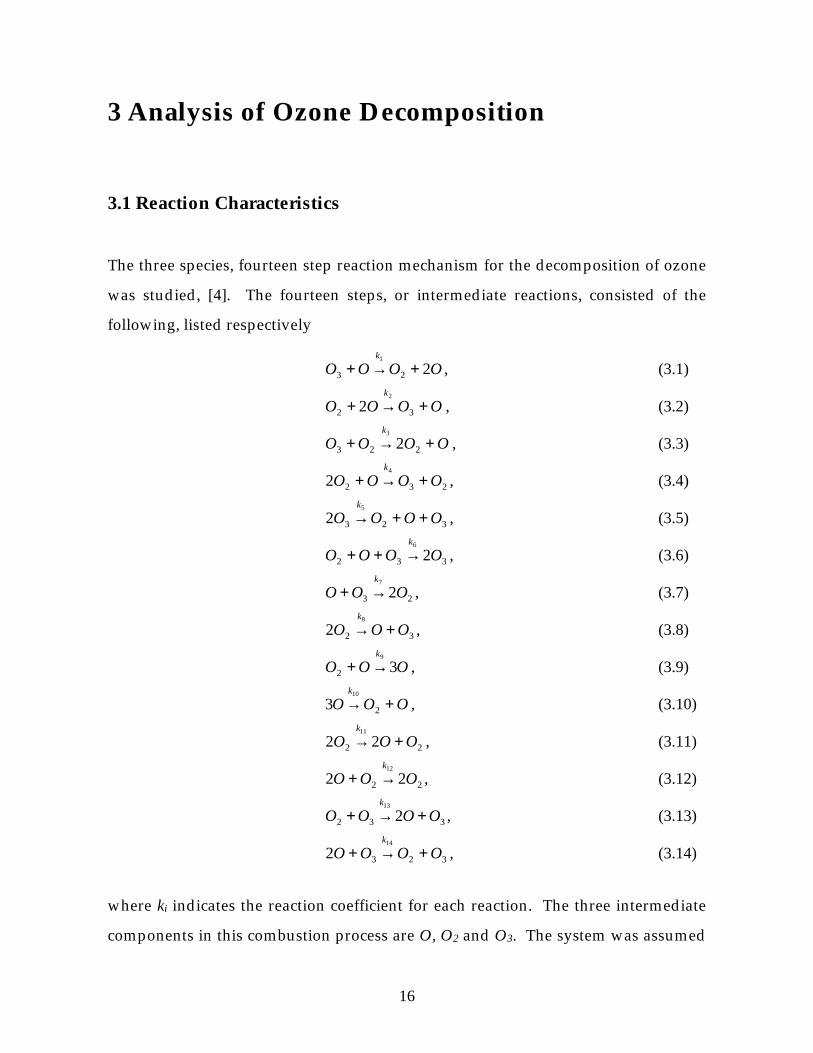
The three species, fourteen step reaction mechanism for the decomposition of ozone

was studied, [4]. The fourteen steps, or intermediate reactions, consisted of the

following, listed respectively

OOOOk

223

1

+→+ , (3.1)

OOOOk

+→+ 32

2

2 , (3.2)

OOOOk

+→+ 223 23

, (3.3)

232

4

2 OOOOk

+→+ , (3.4)

323

5

2 OOOOk

++→ , (3.5)

332 26

OOOOk

→++ , (3.6)

23 27

OOOk

→+ , (3.7)

32

8

2 OOOk

+→ , (3.8)

OOOk

39

2 →+ , (3.9)

OOOk

+→ 2

10

3 , (3.10)

22 2211

OOOk

+→ , (3.11)

22 2212

OOOk

→+ , (3.12)

332 213

OOOOk

+→+ , (3.13)

323

14

2 OOOOk

+→+ , (3.14)

where ki indicates the reaction coefficient for each reaction. The three intermediate

components in this combustion process are O, O2 and O3. The system was assumed

17

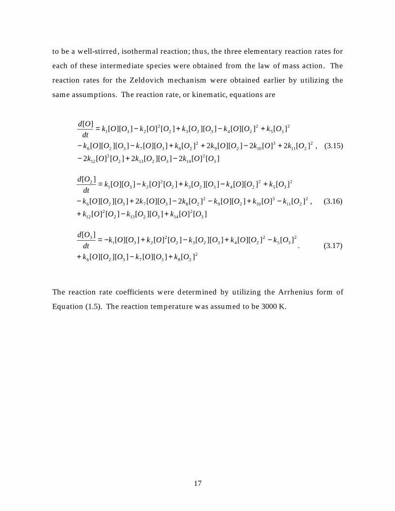
to be a well-stirred, isothermal reaction; thus, the three elementary reaction rates for

each of these intermediate species were obtained from the law of mass action. The

reaction rates for the Zeldovich mechanism were obtained earlier by utilizing the

same assumptions. The reaction rate, or kinematic, equations are

][][2]][[2][][2

][2][2]][[2][]][[]][][[

][]][[]][[][][]][[][

32

14321322

12

2211

31029

22837326

235

2243232

2231

OOkOOkOOk

OkOkOOkOkOOkOOOk

OkOOkOOkOOkOOkdt

Od

−+−

+−++−−

+−+−=

, (3.15)

][][]][[][][

][][]][[][2]][[2]][][[

][]][[]][[][][]][[][

32

14321322

12

2211

31029

22837326

235

2243232

2231

2

OOkOOkOOk

OkOkOOkOkOOkOOOk

OkOOkOOkOOkOOkdt

Od

+−+

−+−−+−

+−+−=

, (3.16)

2

2837326

235

2243232

2231

3

][]][[]][][[

][]][[]][[][][]][[][

OkOOkOOOk

OkOOkOOkOOkOOkdt

Od

+−+

−+−+−=. (3.17)

The reaction rate coefficients were determined by utilizing the Arrhenius form of

Equation (1.5). The reaction temperature was assumed to be 3000 K.

18

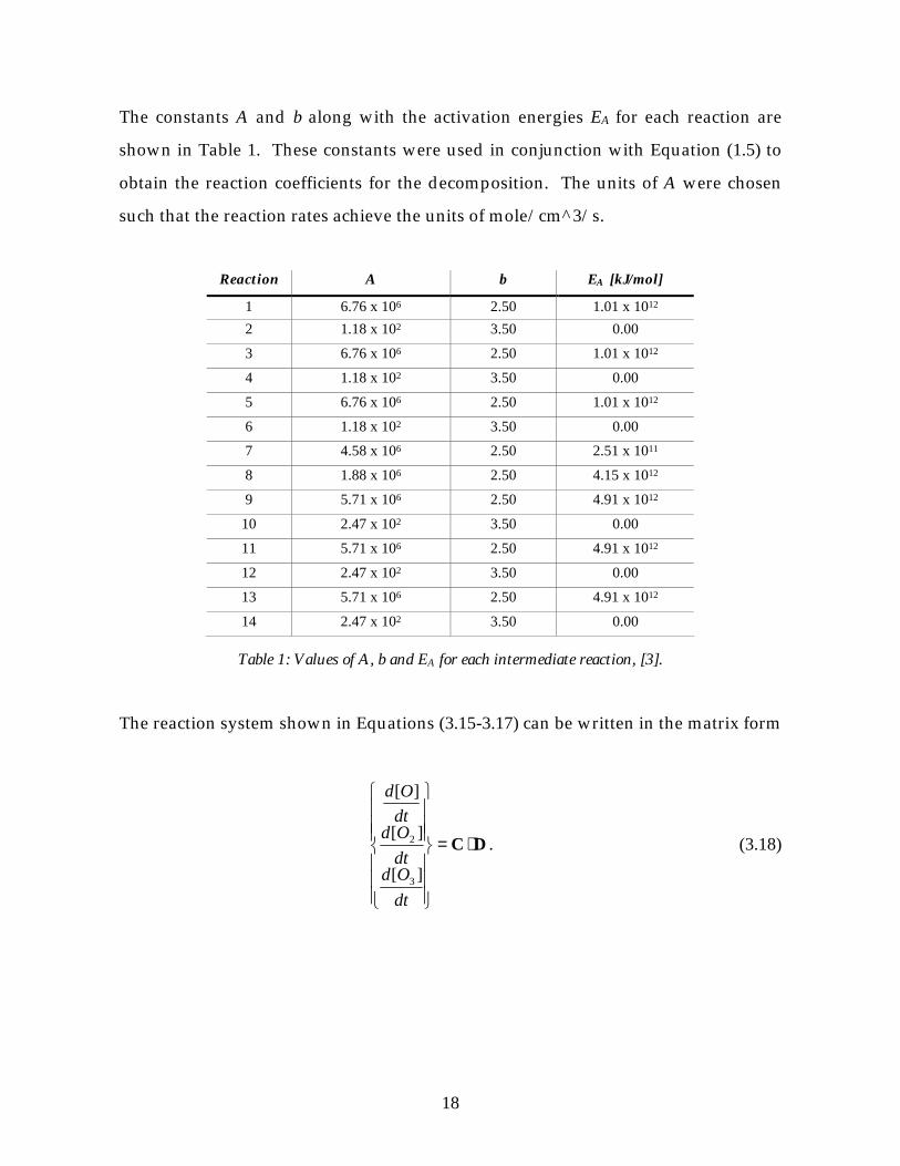
The constants A and b along with the activation energies EA for each reaction are

shown in Table 1. These constants were used in conjunction with Equation (1.5) to

obtain the reaction coefficients for the decomposition. The units of A were chosen

such that the reaction rates achieve the units of mole/cm^3/s.

Reaction A b EA [kJ/mol]

1 6.76 x 106 2.50 1.01 x 1012

2 1.18 x 102 3.50 0.00

3 6.76 x 106 2.50 1.01 x 1012

4 1.18 x 102 3.50 0.00

5 6.76 x 106 2.50 1.01 x 1012

6 1.18 x 102 3.50 0.00

7 4.58 x 106 2.50 2.51 x 1011

8 1.88 x 106 2.50 4.15 x 1012

9 5.71 x 106 2.50 4.91 x 1012

10 2.47 x 102 3.50 0.00

11 5.71 x 106 2.50 4.91 x 1012

12 2.47 x 102 3.50 0.00

13 5.71 x 106 2.50 4.91 x 1012

14 2.47 x 102 3.50 0.00

Table 1: Values of A, b and EA for each intermediate reaction, [3].

The reaction system shown in Equations (3.15-3.17) can be written in the matrix form

DC ⋅=

dt

Oddt

Oddt

Od

][

][

][

3

2 . (3.18)

19

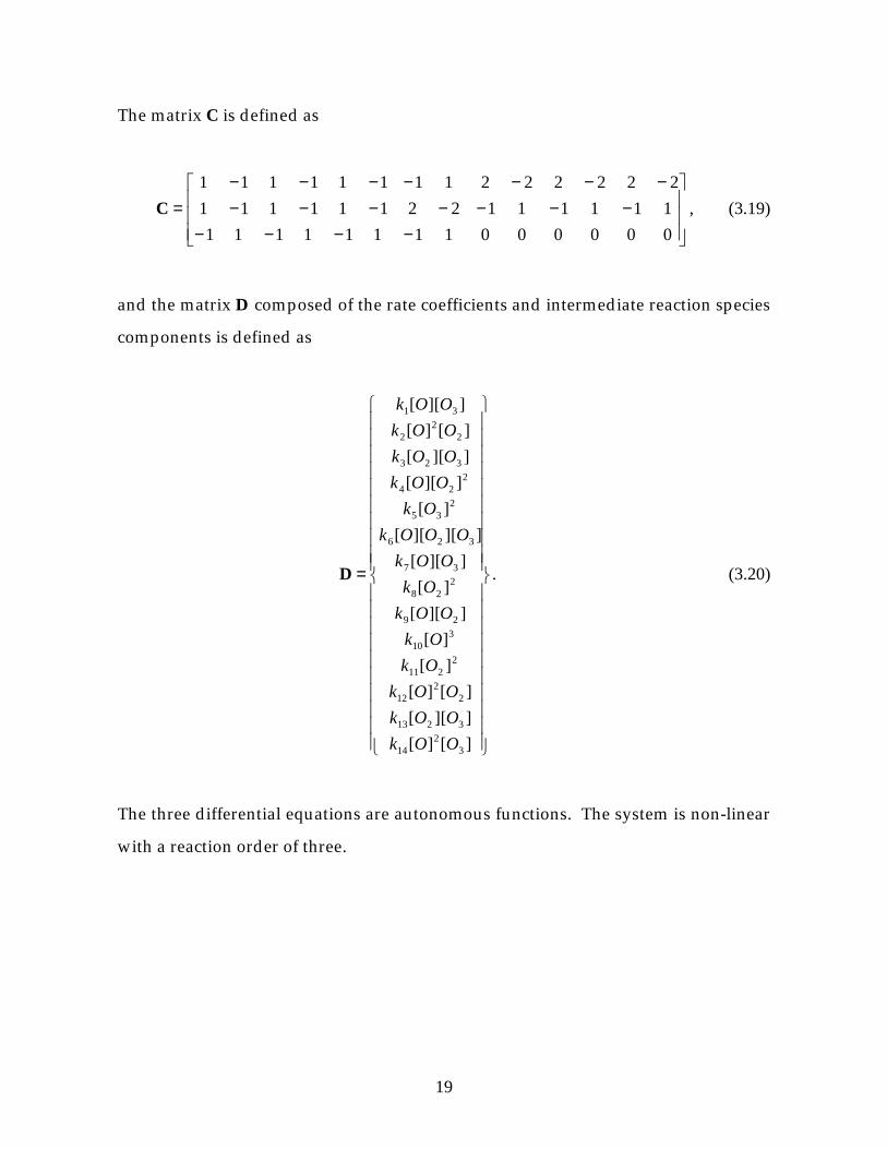
The matrix C is defined as

−−−−−−−−−−−

−−−−−−−=

00000011111111

11111122111111

22222211111111

C , (3.19)

and the matrix D composed of the rate coefficients and intermediate reaction species

components is defined as

=

][][

]][[

][][

][

][

]][[

][

]][[

]][][[

][

]][[

]][[

][][

]][[

32

14

3213

22

12

2211

310

29

228

37

326

235

224

323

22

2

31

OOk

OOk

OOk

Ok

Ok

OOk

Ok

OOk

OOOk

Ok

OOk

OOk

OOk

OOk

D . (3.20)

The three differential equations are autonomous functions. The system is non-linear

with a reaction order of three.

20

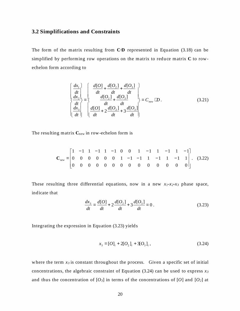
3.2 Simplifications and Constraints

The form of the matrix resulting from C·D represented in Equation (3.18) can be

simplified by performing row operations on the matrix to reduce matrix C to row-

echelon form according to

DC

dt

Od

dt

Od

dt

Oddt

Od

dt

Oddt

Od

dt

Od

dt

Od

dt

dxdt

dxdt

dx

new ⋅=

++

+

++

=

][3

][2

][

][][

][][][

32

32

32

3

2

1

. (3.21)

The resulting matrix Cnew in row-echelon form is

−−−−

−−−−−−=

00000000000000

11111111000000

11111100111111

newC . (3.22)

These resulting three differential equations, now in a new x1-x2-x3 phase space,

indicate that

0][

3][

2][ 323 =++=

dt

Od

dt

Od

dt

Od

dt

dx. (3.23)

Integrating the expression in Equation (3.23) yields

iii OOOx ][3][2][ 323 ++= , (3.24)

where the term x3 is constant throughout the process. Given a specific set of initial

concentrations, the algebraic constraint of Equation (3.24) can be used to express x3

and thus the concentration of [O3] in terms of the concentrations of [O] and [O2] at

21

any time during the combustion process. The value of x3 at the initial conditions can

be obtained by utilizing Equation (3.24) for a given set of initial concentration and

according to Equation (3.23) and Equation (3.24), that value remains constant

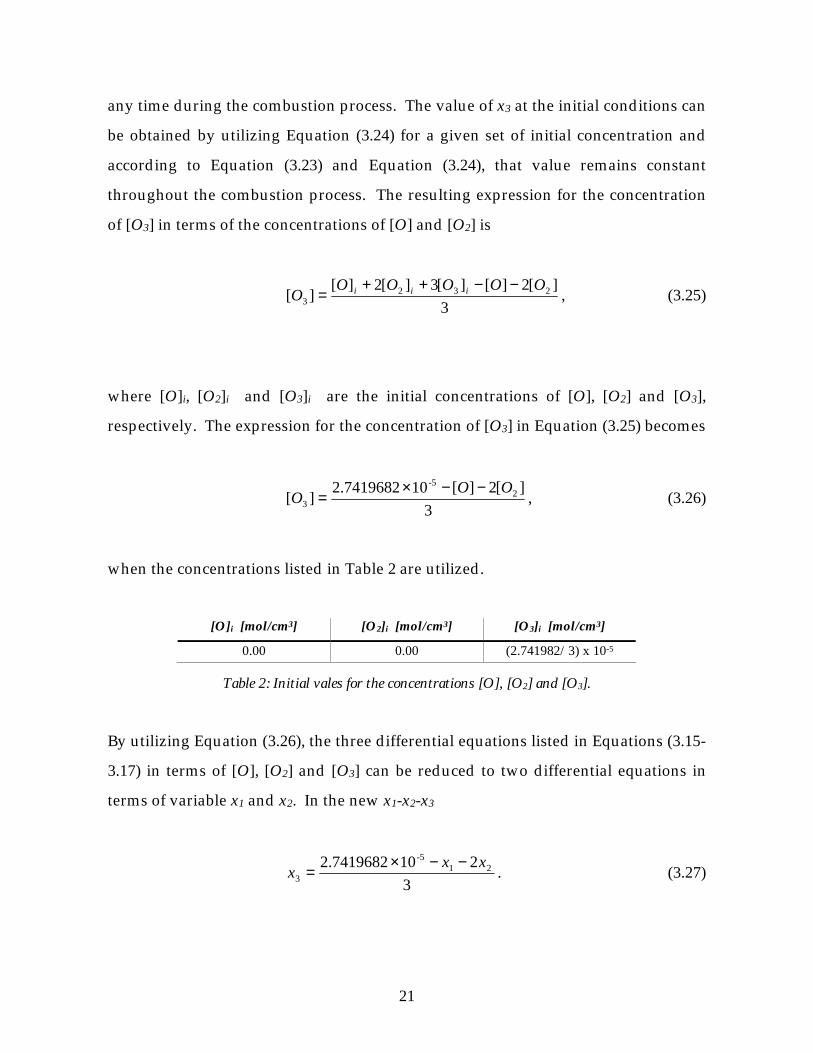
throughout the combustion process. The resulting expression for the concentration

of [O3] in terms of the concentrations of [O] and [O2] is

3

][2][][3][2][][ 232

3

OOOOOO iii −−++

= , (3.25)

where [O]i, [O2]i and [O3]i are the initial concentrations of [O], [O2] and [O3],

respectively. The expression for the concentration of [O3] in Equation (3.25) becomes

3

][2][102.7419682][ 2

-5

3

OOO

−−×= , (3.26)

when the concentrations listed in Table 2 are utilized.

[O]i [mol/cm3] [O2]i [mol/cm3] [O3]i [mol/cm3]

0.00 0.00 (2.741982/3) x 10-5

Table 2: Initial vales for the concentrations [O], [O2] and [O3].

By utilizing Equation (3.26), the three differential equations listed in Equations (3.15-

3.17) in terms of [O], [O2] and [O3] can be reduced to two differential equations in

terms of variable x1 and x2. In the new x1-x2-x3

3

2102.7419682 21-5

3

xxx

−−×= . (3.27)

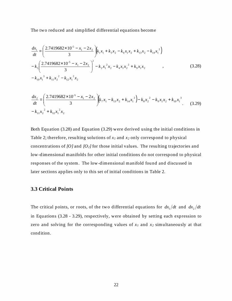
22

The two reduced and simplified differential equations become

( )

22

1122

2113

110

2192

21422

12

2

215-

5

21142132162311

21-5

1

3

2102.7419682

3

2102.7419682

xxkxkxk

xxkxxkxxkxx

k

xkxkxxkxkxkxx

dt

dx

−+−

+−−

−−×−

−+−+

−−×=

, (3.28)

( )2

2112

2211

3110219

228

211421317

21-5

2

3

2102.7419682

xxkxk

xkxxkxkxkxkxkxx

dt

dx

+−

+−−+−

−−×=

. (3.29)

Both Equation (3.28) and Equation (3.29) were derived using the initial conditions in

Table 2; therefore, resulting solutions of x1 and x2 only correspond to physical

concentrations of [O] and [O2] for those initial values. The resulting trajectories and

low-dimensional manifolds for other initial conditions do not correspond to physical

responses of the system. The low-dimensional manifold found and discussed in

later sections applies only to this set of initial conditions in Table 2.

3.3 Critical Points

The critical points, or roots, of the two differential equations for dtdx1 and dtdx2

in Equations (3.28 - 3.29), respectively, were obtained by setting each expression to

zero and solving for the corresponding values of x1 and x2 simultaneously at that

condition.

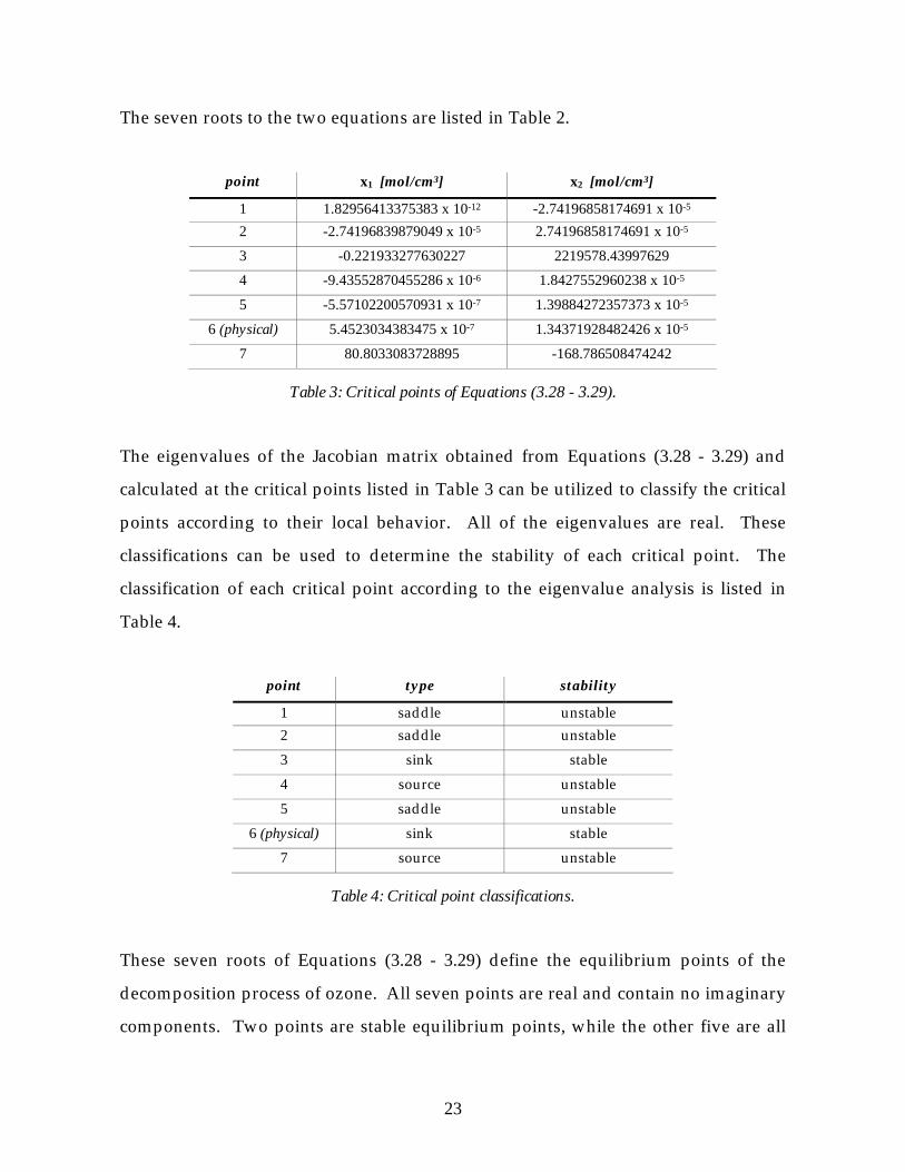
23

The seven roots to the two equations are listed in Table 2.

point x1 [mol/cm3] x2 [mol/cm3]

1 1.82956413375383 x 10-12 -2.74196858174691 x 10-5

2 -2.74196839879049 x 10-5 2.74196858174691 x 10-5

3 -0.221933277630227 2219578.43997629

4 -9.43552870455286 x 10-6 1.8427552960238 x 10-5

5 -5.57102200570931 x 10-7 1.39884272357373 x 10-5

6 (physical) 5.4523034383475 x 10-7 1.34371928482426 x 10-5

7 80.8033083728895 -168.786508474242

Table 3: Critical points of Equations (3.28 - 3.29).

The eigenvalues of the Jacobian matrix obtained from Equations (3.28 - 3.29) and

calculated at the critical points listed in Table 3 can be utilized to classify the critical

points according to their local behavior. All of the eigenvalues are real. These

classifications can be used to determine the stability of each critical point. The

classification of each critical point according to the eigenvalue analysis is listed in

Table 4.

point type stability

1 saddle unstable

2 saddle unstable

3 sink stable

4 source unstable

5 saddle unstable

6 (physical) sink stable

7 source unstable

Table 4: Critical point classifications.

These seven roots of Equations (3.28 - 3.29) define the equilibrium points of the

decomposition process of ozone. All seven points are real and contain no imaginary

components. Two points are stable equilibrium points, while the other five are all

24

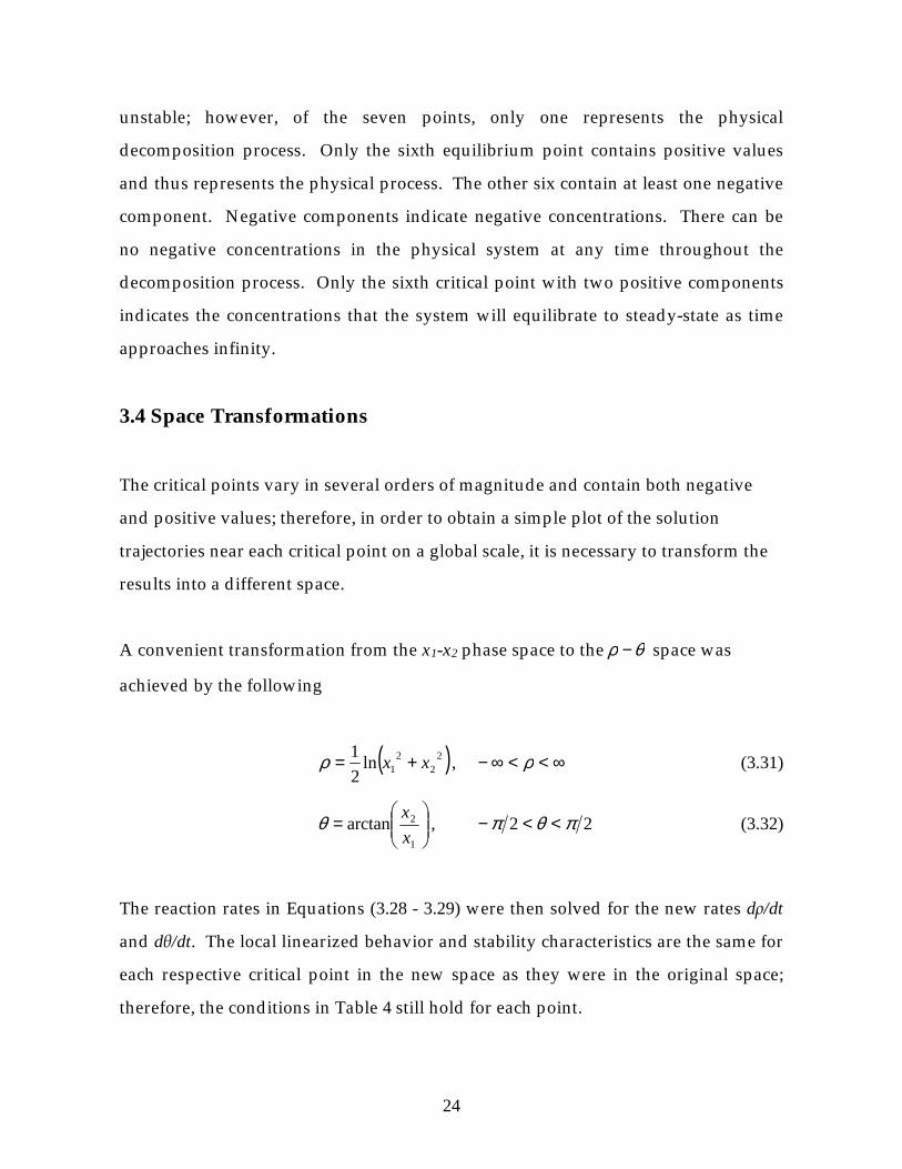
unstable; however, of the seven points, only one represents the physical

decomposition process. Only the sixth equilibrium point contains positive values

and thus represents the physical process. The other six contain at least one negative

component. Negative components indicate negative concentrations. There can be

no negative concentrations in the physical system at any time throughout the

decomposition process. Only the sixth critical point with two positive components

indicates the concentrations that the system will equilibrate to steady-state as time

approaches infinity.

3.4 Space Transformations

The critical points vary in several orders of magnitude and contain both negative

and positive values; therefore, in order to obtain a simple plot of the solution

trajectories near each critical point on a global scale, it is necessary to transform the

results into a different space.

A convenient transformation from the x1-x2 phase space to the θρ − space was

achieved by the following

( )22

21ln

2

1xx +=ρ , ∞<<∞− ρ (3.31)

=

1

2arctanx

xθ , 22 πθπ <<− (3.32)

The reaction rates in Equations (3.28 - 3.29) were then solved for the new rates dρ/dt

and dθ/dt. The local linearized behavior and stability characteristics are the same for

each respective critical point in the new space as they were in the original space;

therefore, the conditions in Table 4 still hold for each point.

25

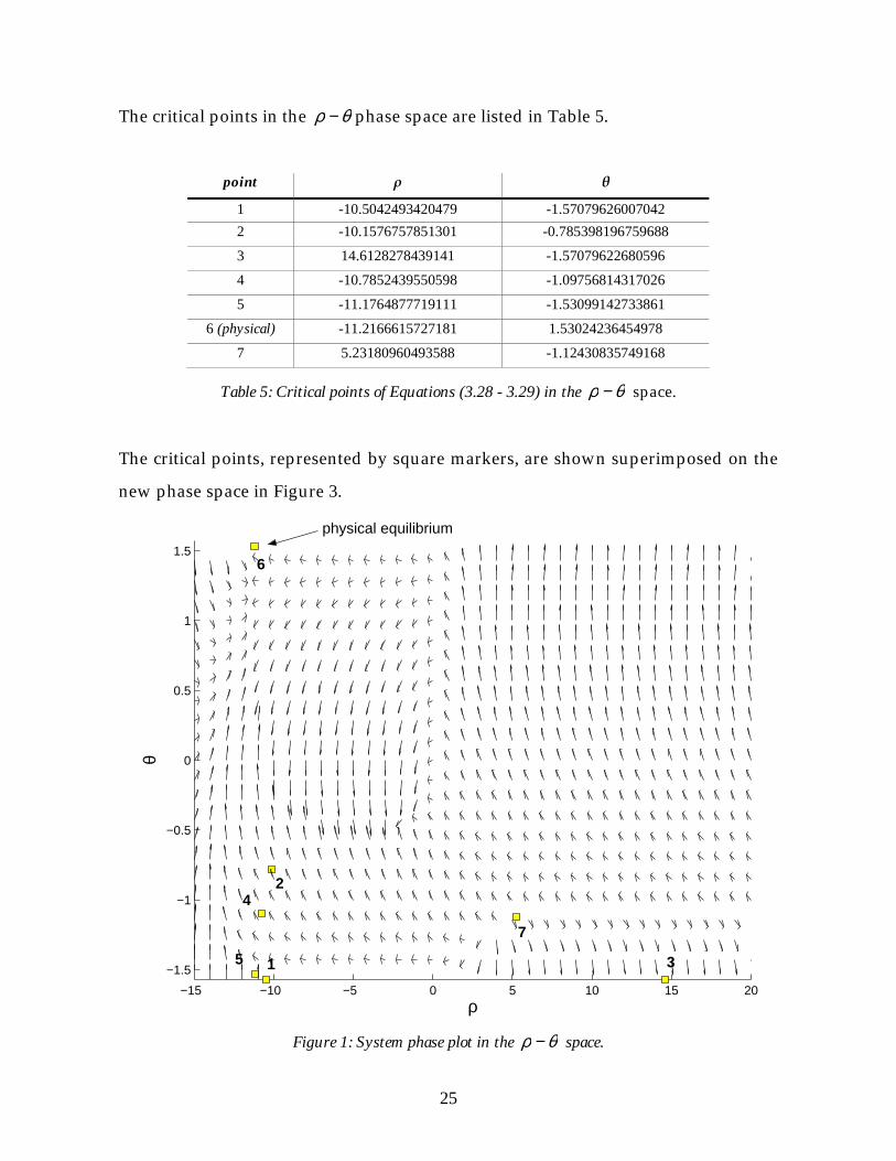
The critical points in the θρ − phase space are listed in Table 5.

point ρ θ

1 -10.5042493420479 -1.57079626007042

2 -10.1576757851301 -0.785398196759688

3 14.6128278439141 -1.57079622680596

4 -10.7852439550598 -1.09756814317026

5 -11.1764877719111 -1.53099142733861

6 (physical) -11.2166615727181 1.53024236454978

7 5.23180960493588 -1.12430835749168

Table 5: Critical points of Equations (3.28 - 3.29) in the θρ − space.

The critical points, represented by square markers, are shown superimposed on the

new phase space in Figure 3.

−15 −10 −5 0 5 10 15 20

−1.5

−1

−0.5

0

0.5

1

1.5

ρ

θ

physical equilibrium

6

24

7

1 5 3

Figure 1: System phase plot in the θρ − space.

26

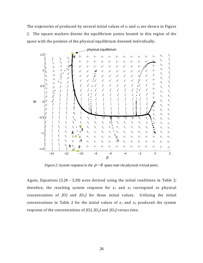
The trajectories of produced by several initial values of x1 and x2 are shown in Figure

2. The square markers denote the equilibrium points located in this region of the

space with the position of the physical equilibrium denoted individually.

−14 −12 −10 −8 −6 −4 −2 0 2

−1.5

−1

−0.5

0

0.5

1

1.5

ρ

θ

4 2

5 1

6

physical equilibrium

Figure 2: System response in the θρ − space near the physical critical point.

Again, Equations (3.28 - 3.29) were derived using the initial conditions in Table 2;

therefore, the resulting system response for x1 and x2 correspond to physical

concentrations of [O] and [O2] for those initial values. Utilizing the initial

concentrations in Table 2 for the initial values of x1 and x2 produced the system

response of the concentrations of [O], [O2] and [O3] versus time.

27

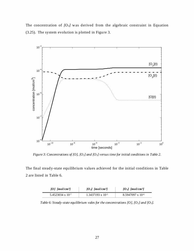
The concentration of [O3] was derived from the algebraic constraint in Equation

(3.25). The system evolution is plotted in Figure 3.

10−10

10−8

10−6

10−4

10−2

100

10−8

10−7

10−6

10−5

10−4

time [seconds]

conc

entr

atio

n [m

ol/c

m3 ]

[O2](t)

[O3](t)

[O](t)

Figure 3: Concentrations of [O], [O2] and [O3] versus time for initial conditions in Table 2.

The final steady-state equilibrium values achieved for the initial conditions in Table

2 are listed in Table 6.

[O] [mol/cm3] [O2] [mol/cm3] [O3] [mol/cm3]

5.4523034 x 10-7 1.3437193 x 10-5 8.5947097 x 10-6

Table 6: Steady-state equilibrium vales for the concentrations [O], [O2] and [O3].

28

3.5 System Response

The trajectories all approach the same steady-state equilibrium point as time

increases. This point is the one physical equilibrium point. This point is a stable

sink, meaning that for any set of physical initial values of x1 and x2, the values of x1

and x2 will approach the physical equilibrium values as time approaches infinity

since the system models the real combustion process of ozone. Physical initial

concentrations will not lead to negative non-physical results in the laboratory. The

eigenvalues and associated eigenvectors evaluated at the physical equilibrium point

indicate the time-scale and approach direction of the trajectories near the

equilibrium point. This same analysis technique applied at each time increment

along the solution trajectory will yield the time-scale at each point on the trajectory.

As time approaches infinity, the corresponding time-scale increases towards a finite

value as the corresponding eigenvalue approaches a finite negative value. The

solution approaches the zero-dimension manifold, one point, in the phase space.

Before the trajectories in Figure 2 reach the zero-dimensional manifold, the

equilibrium point, they approach the one-dimensional manifold. This manifold is a

line in the phase space and observable in Figure 2. The trajectories approach this

line when slow time-scales dominate the system. As the dominat time-scale length

decreases, the resulting manifolds increase in dimension and become impossible to

represent via the phase plot; therefore, the most important manifold and most easily

understood is a low-dimensional manifold.

None of the initial conditions used to generate the trajectories displayed in Figure 2

lie on the low-dimensional manifold. If an initial value lies on a manifold, the

resulting solution response will not deviate from that manifold. For example, if a set

of initial conditions corresponded precisely with the physical equilibrium point, the

resulting solution trajectory would never deviate from that point at any time. The

29

solution trajectory would be simply a point. Similarly, if a set of initial conditions

corresponded to a point on the manifold, the resulting solution trajectory would

mimic the space, a curve in this case, that defines that particular manifold.

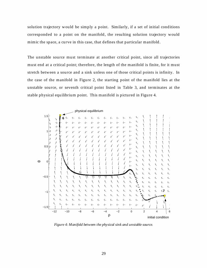
The unstable source must terminate at another critical point, since all trajectories

must end at a critical point; therefore, the length of the manifold is finite, for it must

stretch between a source and a sink unless one of those critical points is infinity. In

the case of the manifold in Figure 2, the starting point of the manifold lies at the

unstable source, or seventh critical point listed in Table 3, and terminates at the

stable physical equilibrium point. This manifold is pictured in Figure 4.

−12 −10 −8 −6 −4 −2 0 2 4 6

−1.5

−1

−0.5

0

0.5

1

1.5

ρ

θ

physical equilibrium

6

initial condition

7

Figure 4: Manifold between the physical sink and unstable source.

30

As discussed earlier, trajectories approach this manifold when the response is

dominated by slowest time-scales. The solution components with faster time-scales

are thus dominated by the slowest time-scale component and quickly approach the

low-dimensional manifold. The eigenvectors at each point in the space indicate the

local system response direction. Given that the magnitude of the time-scale

corresponds to the inverse of each component of the associated eigenvalues, the

largest eigenvalue corresponding to the slowest time-scale of the system would

indicate the local behavior – notably the direction of the trajectory – for the response.

3.6 Manifold Description

To determine the nature of the manifold between the stable physical equilibrium

and the unstable source, the initial concentrations must be such that they nearly, but

not precisely, equal to the coordinates of the source in the space. Since the source is

a critical point of the system, it is also a zero-dimensional manifold; yet, unlike the

physical sink, this manifold is in fact repelling and can be demonstrated so by

calculating the eigenvectors at that point. The initial conditions must thus fall

slightly away from this critical point.

A local linearized perturbation was used to obtain a new set of initial conditions. If

the initial x1 is selected arbitrarily by utilizing a small change between this condition

and the x1 condition at the source, the corresponding x2 can be determined by setting

the slope for a line. For this point to reside on the one-dimensional manifold as

desired, the slope must be equal to that of the eigenvector which has the least

negative eigenvalue indicative of the slowest time-scale. Since the eigenvalues are

inversely proportional to the time-scales, the smallest of the eigenvalues would

correspond to the slowest time-scale. And since the sink is repelling, the eigenvector

is negative and the slope of the line is indeed negative as well. The sink location and

initial conditions located on the one-dimensional manifold are listed in Table 7.

31

point ρ θ

7 (sink) 5.23180960493587 -1.12430835749168

initial conditions 5.23167169426310 -1.12424400000000

Table 7: Sink location and initial conditions located on the one-dimensional manifold.

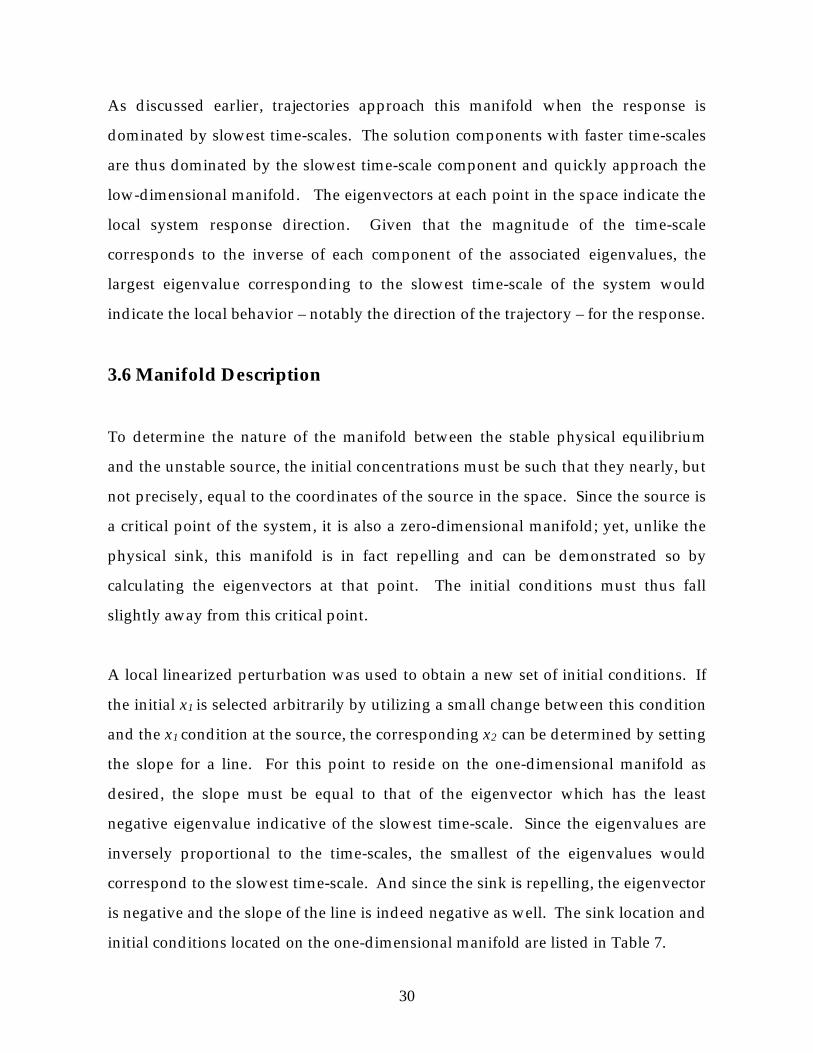
The manifold extending from the unstable source to the stable sink is shown in

Figure 4. The evolution of the ρ and θ concentrations in θρ − space versus time for

initial conditions in Table 7 is shown in Figure 5.

Figure 5: The concentrations in θρ − space versus time for initial conditions in Table 7.

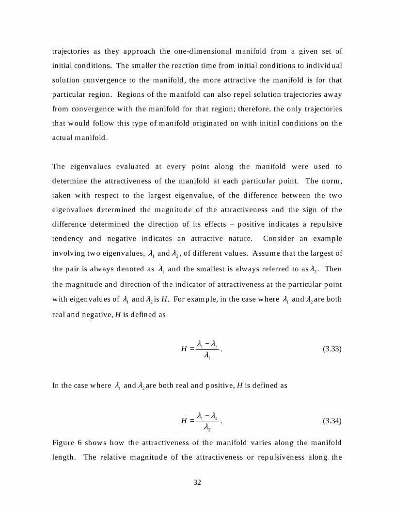
Regions of the manifold can be classified according to their relative attractiveness.

The attractiveness of the manifold is reflected in the size of the time-scales for the

32

trajectories as they approach the one-dimensional manifold from a given set of

initial conditions. The smaller the reaction time from initial conditions to individual

solution convergence to the manifold, the more attractive the manifold is for that

particular region. Regions of the manifold can also repel solution trajectories away

from convergence with the manifold for that region; therefore, the only trajectories

that would follow this type of manifold originated on with initial conditions on the

actual manifold.

The eigenvalues evaluated at every point along the manifold were used to

determine the attractiveness of the manifold at each particular point. The norm,

taken with respect to the largest eigenvalue, of the difference between the two

eigenvalues determined the magnitude of the attractiveness and the sign of the

difference determined the direction of its effects – positive indicates a repulsive

tendency and negative indicates an attractive nature. Consider an example

involving two eigenvalues, 1λ and 2λ , of different values. Assume that the largest of

the pair is always denoted as 1λ and the smallest is always referred to as 2λ . Then

the magnitude and direction of the indicator of attractiveness at the particular point

with eigenvalues of 1λ and 2λ is H. For example, in the case where 1λ and 2λ are both

real and negative, H is defined as

1

21

λλλ −

=H . (3.33)

In the case where 1λ and 2λ are both real and positive, H is defined as

2

21

λλλ −

=H . (3.34)

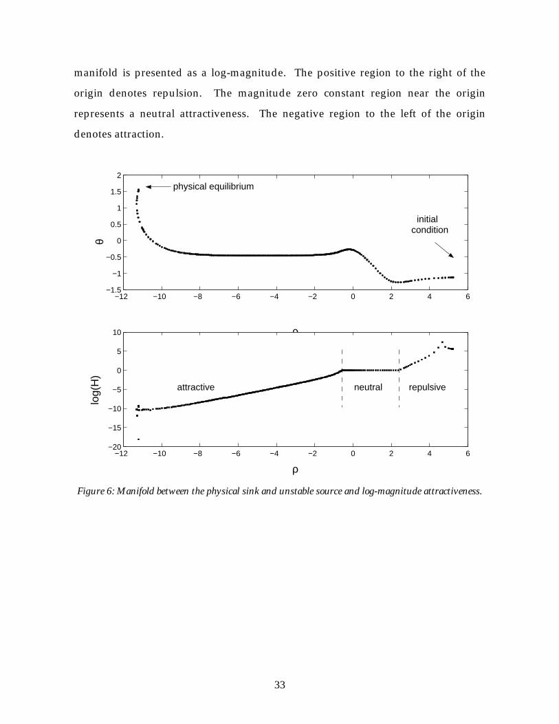
Figure 6 shows how the attractiveness of the manifold varies along the manifold

length. The relative magnitude of the attractiveness or repulsiveness along the

33

manifold is presented as a log-magnitude. The positive region to the right of the

origin denotes repulsion. The magnitude zero constant region near the origin

represents a neutral attractiveness. The negative region to the left of the origin

denotes attraction.

−12 −10 −8 −6 −4 −2 0 2 4 6−1.5

−1

−0.5

0

0.5

1

1.5

2

ρ

θ

−12 −10 −8 −6 −4 −2 0 2 4 6−20

−15

−10

−5

0

5

10

ρ

log(

H)

physical equilibrium

initial condition

attractive neutral repulsive

Figure 6: Manifold between the physical sink and unstable source and log-magnitude attractiveness.

34

3 Conclusions

The concentrations of the intermediate molecular species with respect to time during

the isothermal spatially homogeneous decomposition of ozone were utilized to

identify and determine the behavior of the invariant manifold for the system located

between the unstable source and stable physical equilibrium conditions. The

eigensystem analysis used to ascertain the attractiveness of the manifold at every

point along this manifold indicates that the manifold contains a repulsive tendency

near the source and gradually increases in attractiveness as the system response

approaches the physical equilibrium, or steady-state condition.

The reduction of the three elementary reaction rate equations for the three

intermediate elements of the reaction into two equations and the utilization of the

algebraic constraint obtained from linear operations on the elementary reaction rate

equations greatly simplified the integration routine. The algebraic constraint

reduced the number of dependent variables from three representing the

concentrations of O, O2 and O3 to two representing the concentrations of O and O2

for the prescribed initial conditions used in the algebraic constraint to simplify the

equations. This simplification also reduced the size of the phase space and confined

the system trajectories to a two-dimensional plane whereas before the system

response existed in three-dimensional space. Since numerical integration techniques

were used to obtain the system response, the approach discussed and outlined

herein provides a representation of the chemical kinetics of a combustion process of

the system represented by two non-linear ODEs.

Analysis indicated the existence of seven critical points of the elementary reaction

rate equations. All were wholly real without any imaginary components and two

points were stable sinks. Only one point represented an actual physical state that

35

the reaction may achieve. This equilibrium point represented the steady-state

condition for the reaction. The system response and critical points were transformed

from the x1-x2 phase space into the new θρ − space to facilitate the analysis on a

global level. System response trajectories were generated in the phase space and

utilized to determine the location and appearance the one-dimensional manifold

between the physical stable sink and unstable source. The computational time

required to perform the numerical integrations was minimal due to the simplified

nature of the rate equations through the imposition of the algebraic constraint and

reduction in dependent variables. This technique provided an accurate picture of

the system response and invariant manifold characteristics for the decomposition of

ozone, as the only error introduced into the system response arose from the

precision limitations of the computational routine.

36

References

1. Turns, S. R., An Introduction to Combustion: Concepts and Applications, pp. 111-

143, McGraw-Hill, (2000).

2. Glassmaker, N. J., “ILDM Method for Rational Simplification of Chemical

Kinetics,” AME 499 Fluids Report, University of Notre Dame, (1999).

3. Singh, S., Powers, J. M., Paolucci, S., “On Slow Manifolds of Chemically

Reactive Systems,” Journal of Chemical Physics, Vol. 117, pp. 1492-1496, (2002).

4. Margolis, S. B., “Time Dependent Solution of a Premixed Laminar Flame,”

Journal of Computational Physics, Vol. 27, pp. 410-427, (1978).