Embed Size (px)
Citation preview
Calculus for Everyone (Chapters 1 - 11)
S. R. Kingan
c© 2018, S. R. Kingan
All right reserved.
Contents
Preface iii
Chapter 1. What is a Limit? 1
Chapter 2. Continuous Functions 16
Chapter 3. Techniques for Finding Limits 22
Chapter 4. What is a Derivative? 33
Chapter 5. Derivative Rules and Formulas 47
Chapter 6. More Derivative Formulas 63
Chapter 7. Implicit Di�erentiation 75
Chapter 8. L'Hôpital's Rule 84
Chapter 9. Related Rates 90
Chapter 10. Maxima and Minima 100
Chapter 11. Optimization 113
ii

Preface
As its camp�res glow against the dark, every culture tells stories to itselfabout how the gods lit up the morning sky and set the wheel of beinginto motion. The great scienti�c culture of the west - our culture - is noexception. The calculus is the story this world �rst told itself as it becamethe modern world. - David Berlinski
But how is one to make a scientist understand that there is somethingunalterably deranged about di�erential calculus, quantum theory, or theobscene and so inanely liturgical ordeals of the precession of the equinoxes.- Antonin Artaud (said tongue-in-cheek no doubt)
Regardless of your Calculus pursuasion, like Shakespeare's plays everyone should seeCalculus at least once in their schooling. Caculus is the language of movement. Anyone whowishes to learn Calculus can learn it. However, not everyone can read a Calculus textbook.This is because most math textbooks are written for the instructor, not the student. Theyare comprehensive tomes, often over 500 pages, and written so that an instructor can makea selection of material for a semester based on personal taste. This book is for the studenttaking Calculus. The selection of material is already made. All the material presented isessential (besides the nerdy jokes and cultural asides).
The advantage of having a book like this as the textbook is that the instructor canexpect the students to actually read the material and come prepared to class having donethe �readings.� Every e�ort is made to make the book readable. The standard textbookformat where Chapter 1 is divided into sections, and sections into subsections and so on,is eschewed in favor of a more narrative style. The standard format with examples labeled1.3.1.2 is good for an instructor who uses the textbook as a reference manual, but to thestudent it reads like a dry code manual. In this book there are no sections and subsections,just chapters like in a novel.
The graphs in this book are produced using wolframalpha.com which is the free versionof Mathematica. This website has a Google like interface. An equation or function can beentered into the box somewhat imprecisely and it will understand and solve it or sketchit. This is a bigger advantage than it sounds. Having to know precise codes for everythingmakes using graphic calculators and computer algebra systems tedious. Even one bracketout of place causes an error. Free software that is intelligent enough to understand whatthe user intends to type is a game-changer in the way students can learn Precalculus andCalculus.
Figures in the book have a simple appearance to emphasize that they can be drawn byhand. Modern textbook have an impressive array of pictures and �gures that are not only
iii

iv PREFACE
attention-de�cit inducing, but also leave the reader with the sense that he could never drawthe �gures himself. Conventional wisdom supposes that some people understand informationbetter when it is presented with words, whereas others prefer a more visual approach. Butin mathematics, the visual approach is not just an alternate pedagogical approach, it isessential. We understand mathematical objects in terms of pictures. For example, theobject y = x2 is not really meaningful unless it is recognized as the parabola with vertex(0, 0) that is symmetric about the y-axis. Arguably we use words to convey the pictures wehave in mind.
Right from the beginning students are encouraged to �nd solutions to problems on theirown using freely available resources. The exercises do not come with a solution sheet. Inmost cases students can use wolframalpha.com to get the solutions. Students should learn towork with friends to check their solution and with practice become con�dent that their workis correct. This book works well for teaching strategies such as �collaborative learning� and�team-based learning,� which emphasize working in groups. It also works well for the ��ippedclassroom,� where the students have to read and understand each chapter independentlybefore it is presented in the classroom and class-time is spent discussing the material notteaching it. It may not be a good idea to completely forgo the old-fashioned lecture styleof teaching mathematics in favor of a new strategy. However, including active learningcomponents like allowing students to ask questions, requiring them to read ahead and comeprepared to discuss the material, and giving team-based quizzes are e�ective teaching andlearning tools.
This book has few word problems. Word problems in math textbooks are proxy forreal-world applications. They are contrived and often confusing paragraphs that supposedlycapture a situation where math is applied to a real-world situation, but they manage toremove all the fun out of both the math and the application. The di�culty with doingapplications properly in a math class is that the applications are discipline speci�c andreqire considerable subject knowledge. There is no time in the mathematics classroom togive students a solid application from another discipline, without sacr�cing something, andthat something is usually rigor. The best course of action for students is to �rst work througha few carefully worded problems like the ones in this book to get the ideas straight. As Hardysaid in his 1941 book �A Mathematician's Apology,�
A mathematician, like a painter or a poet, is a maker of patterns. If hispatterns are more permanent than theirs, it is because they are made withideas.
Then, based on interest, follow up by looking at one of the websites that specialize in appli-cations that use Calculus. Don't waste time on arti�cal real-word problems (the oxymoron isunavoidable). Theory and applications must go hand-in-hand despite an educational systemseemingly set up to make this impossible.
Typically Chapters 1 to 12 (chapter 12 is still unwritten) covering limits and derivativescorresponds to a 3 or 4 credit Calculus I course lasting 15 weeks, and integration and series iscovered in a Calculus II course. There is considerable sca�olding of topics to gradually movestudents toward a stronger understanding, ultimately making them independent learners.This is why the proofs of theorems appear in a separate chapter at the end. These proofs are

PREFACE v
essential for Calculus II, but not essential for a student who just wants a taste of Caculus.The proofs become more meaningful after they are used in problem solving. So the focusthroughout is solving problems.
Many students require only a Calculus I course. Putting students who require onlyCalculus I in the same class as those who require Calculus I and II causes major problems.If limits and derivatives are covered rigorously, then students never see the beauty andimportance of integration. If a non-rigorous approach is adopted, then the students goingon to Calculus II have too weak a background to succeed. It is better to o�er studentswho require only one calculus course a �Survey of Calculus� that covers both derviatives andintegrals and is known from the beginning to be a �mile-wide and inch-deep.� This bookcan be used for such a course by studying limits without emphasizing techniques for �ndingthem, omitting all proofs as well as the more complicated derivatives and integrals, andcompletely omitting series. Throughout there are footnotes to help students navigate thematerial in a non-rigourous fashion. The hope is that such students become interested inknowing things thoroughly when they realize they can read a math textbook on their own.
We will end with Steven Strogatz's description of Calculus taken from his wonderful NewYork Times article �Change we can believe in� that should be required reading for everyone.
Calculus is the mathematics of change. It describes everything from thespread of epidemics to the zigs and zags of a well-thrown curveball. Thesubject is gargantuan - and so are its textbooks. Many exceed 1,000 pagesand work nicely as doorstops. But within that bulk you'll �nd two ideasshining through. All the rest, as Rabbi Hillel said of the Golden Rule, is justcommentary. Those two ideas are the �derivative� and the �integral.� Eachdominates its own half of the subject, named in their honor as di�erentialand integral calculus. Roughly speaking, the derivative tells you how fastsomething is changing; the integral tells you how much it's accumulating.They were born in separate times and places: integrals, in Greece around250 B.C.; derivatives, in England and Germany in the mid-1600s. Yet in atwist straight out of a Dickens novel, they've turned out to be blood relatives- though it took almost two millennia to see the family resemblance.
The author thanks Professor Miriam Deutch for taking the lead on OpenSource@CUNY, thefaculty and technical sta� on the team, and Brooklyn College for giving a 3-credit courserelease to write yet another commentary on one of the greatest discoveries of humanity.
CHAPTER 1
What is a Limit?
Calculus is the study of change. It is a way of making sense of the world we live in. If thisutilitarian argument doesn't appeal to you, then learn Calculus because it is one of the greatachievements of humanity. Study it like you would a great piece of artwork, except that itisn't tangible and gets drawn in your head with the help of ideas. It does, however, haveconsiderable prerequistes including algebra, geometry, and trigonometry grouped togetherunder the umbrella term �Precalculus.� So, assuming you have taken a Precalculus courselet's begin, as the King of Hearts from Alice in Wonderland said, �at the beginning.� whichreally isn't the begining at all as we will see later on, but we have to start somewhere.
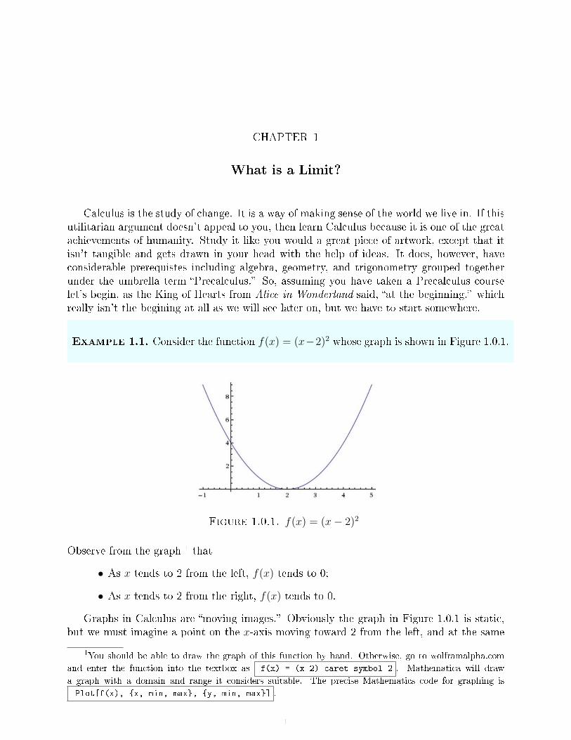
Example 1.1. Consider the function f(x) = (x−2)2 whose graph is shown in Figure 1.0.1.
Figure 1.0.1. f(x) = (x− 2)2
Observe from the graph 1 that
• As x tends to 2 from the left, f(x) tends to 0;
• As x tends to 2 from the right, f(x) tends to 0.
Graphs in Calculus are �moving images.� Obviously the graph in Figure 1.0.1 is static,but we must imagine a point on the x-axis moving toward 2 from the left, and at the same
1You should be able to draw the graph of this function by hand. Otherwise, go to wolframalpha.com
and enter the function into the textbox as f(x) = (x-2) caret symbol 2 . Mathematica will draw
a graph with a domain and range it considers suitable. The precise Mathematics code for graphing is
Plot[f(x), {x, min, max}, {y, min, max}] .
1

2 1. WHAT IS A LIMIT?
time a point on the graph of f(x) moving along the curve toward 0. We use the symbol 2−
to denote the phrase �2 from the left� and 2+ to denote the phrase �2 from the right.� Weuse → for the phrase �tends to.� The above observation in symbols becomes
• As x −→ 2−, f(x) −→ 0;
• As x −→ 2+, f(x) −→ 0.
We further shorten it using the �limit� notation as follows:
• limx→2−
f(x) = 0 (read as �limit as x tends to 2 minus of f of x is 0�);
• limx→2+
f(x) = 0.
We call limx→2−
f(x) = 0 the left limit and limx→2+
f(x) = 0 the right limit. Observe that the
left limit and right limit both exist and are equal. So
limx→2−
f(x) = limx→2+
f(x) = 0.
In this case we say the limit exists and we write
limx→2
f(x) = 0.
Example 1.2. Consider the piecewise function g(x) =
{3x if x 6= 2
8 if x = 2whose graph is shown
in Figure 1.0.2.
Figure 1.0.2. The piecewise function g(x) with a hole at 2
A piecewise function is de�ned in di�erent pieces on the domain; hence the name. Thisfunction g(x) is the line y = 3x with a �hole� in it. The hole exists because 3(2) = 6 but atx = 2 the function takes the value 8. 2
2Piecewise functions have to be entered precisely using Mathematica Code. Enter g(x) as
g(x) = Piecewise[{{3x, x[NotEqual]2}, {8, x=2}}] .
1. WHAT IS A LIMIT? 3
Observe thatlimx→2−
g(x) = 6 and limx→2+
g(x) = 6.
So,limx→2−
g(x) = limx→2+
g(x) = 6.
We say the limit exists and we write
limx→2
g(x) = 6.
Observe that, in the �rst example limx→2
f(x) = f(2) and in the second example limx→2
g(x) 6= g(2)
because limx→2
g(x) = 6 and g(2) = 8. However, in both cases the limit exists.
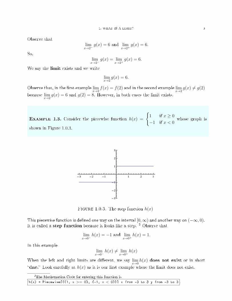
Example 1.3. Consider the piecewise function h(x) =
{1 if x ≥ 0
−1 if x < 0whose graph is
shown in Figure 1.0.3.
Figure 1.0.3. The step function h(x)
This piecewise function is de�ned one way on the interval [0,∞) and another way on (−∞, 0).It is called a step function because it looks like a step. 3 Observe that
limx→0−
h(x) = −1 and limx→0+
h(x) = 1.
In this examplelimx→0−
h(x) 6= limx→0+
h(x)
When the left and right limits are di�erent, we say limx→0
h(x) does not exist or in short
�dne.� Look carefully at h(x) as it is our �rst example where the limit does not exist.
3The Mathematica Code for entering this function is
h(x) = Piecewise[{{1, x >= 0}, {-1, x < 0}}] x from -3 to 3 y from -3 to 3 .
4 1. WHAT IS A LIMIT?
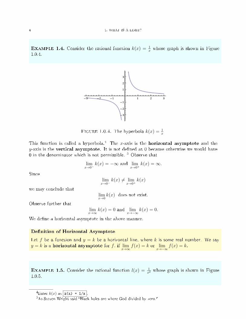
Example 1.4. Consider the rational function k(x) = 1xwhose graph is shown in Figure
1.0.4.
Figure 1.0.4. The hyperbola k(x) = 1x
This function is called a hyperbola.4 The x-axis is the horizontal asymptote and they-axis is the vertical asymptote. It is not de�ned at 0 because otherwise we would have0 in the denominator which is not permissible. 5 Observe that
limx→0−
k(x) = −∞ and limx→0+
k(x) =∞.
Sincelimx→0−
k(x) 6= limx→0+
k(x)
we may conclude thatlimx→0
k(x) does not exist.
Observe further thatlimx→∞
k(x) = 0 and limx→−∞
k(x) = 0.
We de�ne a horizontal asymptote in the above manner.
De�nition of Horizontal Asymptote
Let f be a function and y = k be a horizontal line, where k is some real number. We sayy = k is a horizontal asymptote for f , if lim
x→∞f(x) = k or lim
x→−∞f(x) = k.
Example 1.5. Consider the rational function l(x) = 1x2
whose graph is shown in Figure1.0.5.
4Enter k(x) as k(x) = 1/x .5As Steven Wright said �Black holes are where God divided by zero."

1. WHAT IS A LIMIT? 5
Figure 1.0.5. The hyperbola l(x) = 1x2
Observe thatlimx→0−
l(x) =∞ and limx→0+
l(x) =∞.
In this example, since the left and right limits exist and are the same,
limx→0
l(x) =∞
Note that we are abusing notation slightly when we say the limit is equal to∞ since in�nityis not a number. Some textbooks prefer to use words saying �the limit tends to in�nity.�Other textbooks prefer to be brief and (mis)use the ∞ notation. We will adopt the latterconvention.
We are now ready to formulate a working de�nition of limits.
De�nition of Limit
Let f(x) be a real-valued function de�ned on an open interval containing point a, exceptpossibly at a, and let L be a real number.
(1) If f(x) tends to L as x tends to a from the left, then the left limit exists and wewrite lim
x→a−f(x) = L
(2) If f(x) tends to L as x tends to a from the right, then the right limit exists andwe write lim
x→a+f(x) = L
(3) If the left and right limit both exists and are equal, then the limit exists and wewrite lim
x→af(x) = L
(4) If f(x) tends to L as x tends to ∞, then limx→∞
f(x) = L
This de�nition is what we call an informal de�nition. It will do for now, but soon wewill see why it is inadequate. Let us see some more examples.

6 1. WHAT IS A LIMIT?
Example 1.6. Find the following limits:
(1) limx→2
5
(2) limx→2
3x+ 7
(3) limx→−∞
2x
(4) limx→0
ln(x)
(5) limx→π
2
tanx
(6) limx→0
cotx
(7) limx→0
cscx
(8) limx→∞
tan−1 x
Solution.
(1) The graph of y = 5 is a horizontal straight line (see Figure 1.0.6). No matter whatvalue x takes, whether it is 2 or something else, y is always 5. So lim
x→25 = 5
Figure 1.0.6. The horizontal line y = 5
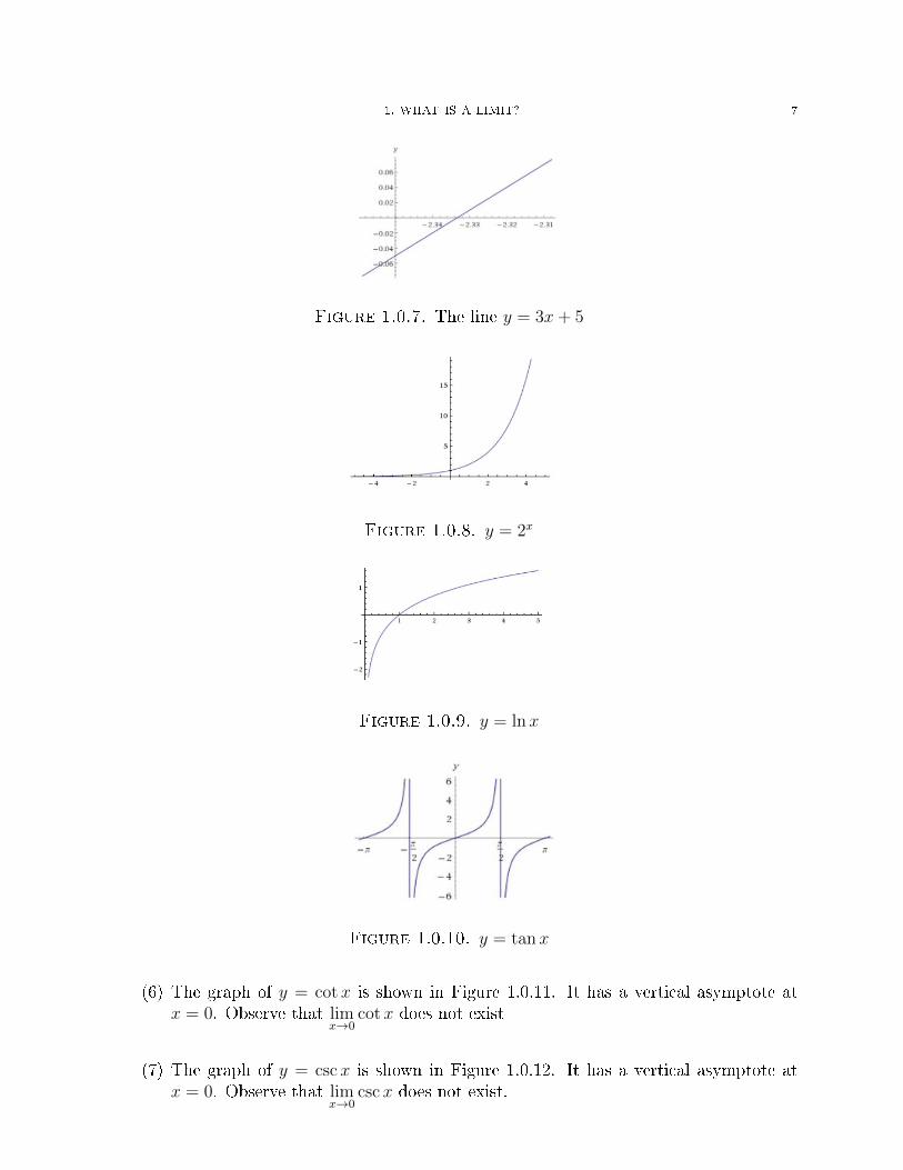
(2) The graph of y = 3x + 7 is the straight line shown in Figure 1.0.7. Observe thatlimx→2
3x+ 7 = 3(2) + 7 = 13.
(3) The graph of y = 2x is shown in Figure 1.0.8. Observe that the x-axis is thehorizontal asymptote. So lim
x→−∞2x = 0.
(4) The graph of y = ln x is shown in Figure 1.0.9. Observe that the y-axis is thevertical asymptote. So lim
x→0lnx = −∞.
(5) The graph of y = tanx is shown in Figure 1.0.10. It has a vertical asymptote atx = π
2. Observe that lim
x→π2−
tanx = −∞ and limx→π
2+
tanx = ∞. So limx→π
2
tan−1 x does
not exist.
1. WHAT IS A LIMIT? 7
Figure 1.0.7. The line y = 3x+ 5
Figure 1.0.8. y = 2x
Figure 1.0.9. y = lnx
Figure 1.0.10. y = tanx
(6) The graph of y = cotx is shown in Figure 1.0.11. It has a vertical asymptote atx = 0. Observe that lim
x→0cotx does not exist
(7) The graph of y = cscx is shown in Figure 1.0.12. It has a vertical asymptote atx = 0. Observe that lim
x→0cscx does not exist.
8 1. WHAT IS A LIMIT?
Figure 1.0.11. y = cotx
Figure 1.0.12. y = cscx
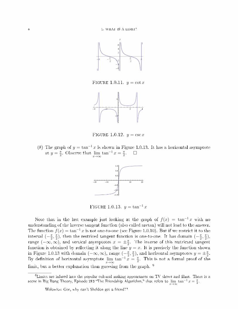
(8) The graph of y = tan−1 x is shown in Figure 1.0.13. It has a horizontal asymptoteat y = π
2. Observe that lim
x→∞tan−1 x = π
2. �
Figure 1.0.13. y = tan−1 x
Note that in the last example just looking at the graph of f(x) = tan−1 x with nounderstanding of the inverse tangent function (also called arctan) will not lead to the answer.The function f(x) = tan−1 x is not one-to-one (see Figure 1.0.10). But if we restrict it to theinterval (−π
2, π2), then the restriced tangent function is one-to-one. It has domain (−π
2, π2),
range (−∞,∞), and vertical asymptotes x = ±π2. The inverse of this restricted tangent
function is obtained by re�ecting it along the line y = x. It is precisely the function shownin Figure 1.0.13 with domain (−∞,∞), range (−π
2, π2), and horizontal asymptotes y = ±π
2.
By de�nition of horizontal asymptote limx→∞
tan−1 x = π2. This is not a formal proof of the
limit, but a better explanation than guessing from the graph. 6
6Limits are infused into the popular cultural making appearances on TV shows and �lms. There is ascene in Big Bang Theory, Episode 213 �The Friendship Algorithm," that refers to lim
x→∞tan−1 x = π
2 .
Wolowitz: Gee, why can't Sheldon get a friend?"

1. WHAT IS A LIMIT? 9
x y = sinxx
±0.1 0.998334166±0.01 0.99998333±0.001 0.999998333±0.0001 0.9999995±0.00001 1.0±0.000001 1.0
Table 1. The behavior of f(x) = sinxx
near x = 0
So far we adopted a highly visual approach to limits. But drawing graphs is not alwayspossible.
Example 1.7. Consider the function f(x) = sinxx
whose graph is shown in Figure 1.0.14(but don't look now).
This is not a function with a well-known shape like the previous functions. How shouldwe �nd lim
x→0
sinxx? One approach is to take values of x closer and closer to 1 and �nd the
corresponding values of sinxx. This is the computational approach and it is illustrated in
Table 1. Observe that as x tends to 0, sinxx
tends to 1. The computational approach suggests
thatlimx→0
sinx
x= 1.
But, how do we know something strange doesn't happen very close to 0. There is clearlysomething stronger than computation needed to say conclusively that the limit is 1.
As mentioned earlier, the graph of f(x) = sinxx
is shown in Figure 1.0.14. The graphsupports our computational intuition that the limit is 1. Are we correct? The answer is yesin this case, and it is quite clear from the graph. However, we are left with a vague sensethat more is needed.
The previous example may suggest that using graphing software will always help in�nding limits. Unfortunately, this is not the case.
Example 1.8. Consider the function f(x) = sin πxwhose graph is shown in Figure 1.0.15.
Judging by this graph, we might hesitantly venture a guess that limx→0
sin πxis 0. Table 2 shows
that our guess is bolstered by computational evidence. If we tried to zoom in to get a clearerpicture of the function's behavior near zero we would get Figure 1.0.16, which is no morehelpful. So are we correct? The answer is no.
limx→0
sinπ
xdoes not exist.
Sheldon: What part of an inverse tangent approaching an asymptote don't you under-stand?

10 1. WHAT IS A LIMIT?
Figure 1.0.14. f(x) = sinxx
Figure 1.0.15. f(x) = sin πx
Figure 1.0.16. A zoomed in view of f(x) = sin πxnear 0
This is because no matter how close x gets to 0 the function f(x) oscillates wildly from -1 to1. This is not based on visual intuition nor computational intuition. A stronger de�nitionis needed and that is the formal de�nition of the limit.

1. WHAT IS A LIMIT? 11
x y = sin πx
1 012
013
014
015
016
0
Table 2. The behavior of f(x) = sin πxnear x = 0
Formal De�nition of Limit
Let f(x) be a real-valued function de�ned on an open interval containing a point a, exceptpossibly at a, and let L be a real number. The statement
limx→a
f(x) = L
means that for every ε > 0, there exists δ > 0, such that
if 0 < |x− a| < δ then |f(x)− L| < ε.
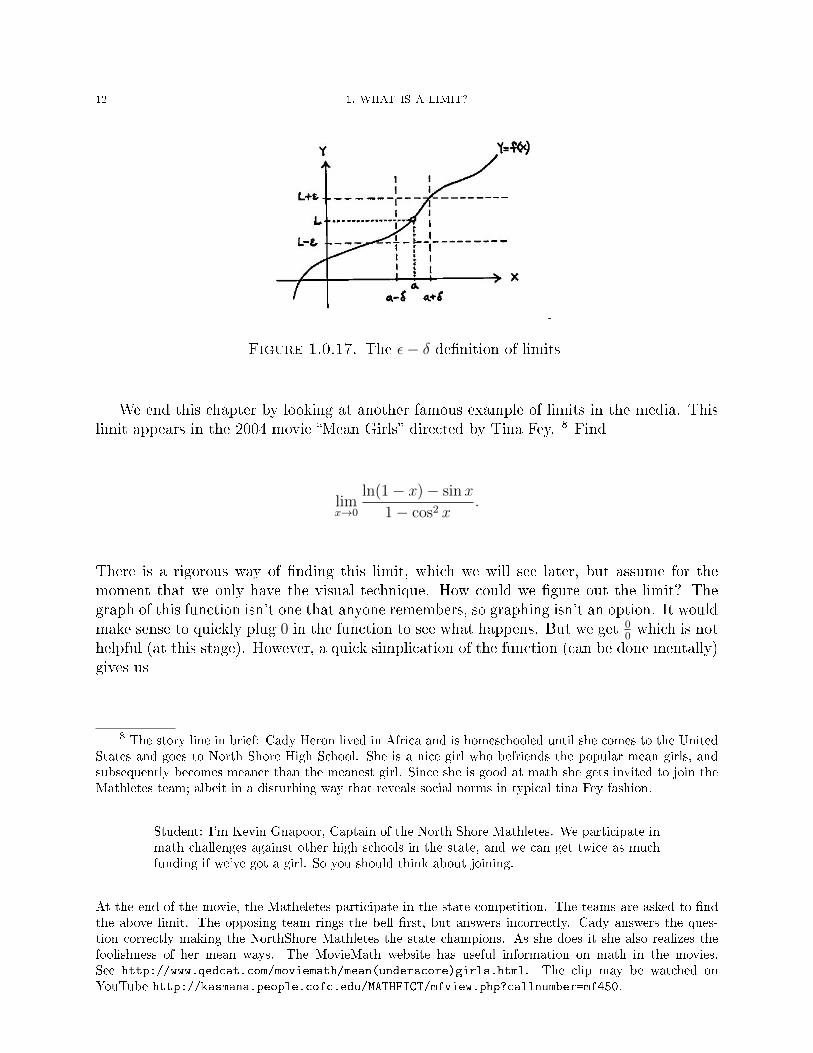
Figure 1.0.17 7 explains the de�nition. For every small number ε such that the distance off(x) to L is less than ε, there is a small number δ such that the distance between x and a isless than δ. Note that |x− a| < δ means x is in the interval (a− δ, a+ δ) and |f(x)−L| < εmeans f(x) is in the interval (L− ε, L+ ε). As the interval around L on the y-axis shrinks,the interval around a on the x-axis shrinks. The box in the center of the �gure also shrinksand captures the limit inside it.
The formal de�nition of limits is mostly outside the scope of this course, but it helps tohave some understanding of it (you will begin an Advanced Calculus with this de�nition).As usual the way to understand something is to work out some examples. The exampleshere are �proofs" and we postpone it till Chapter 12. At this junction it is enough to realizethat something stronger than the visual and computation approach to limits is needed.
7 This �gure is taken from https://www.math.ucdavis.edu/ kouba/CalcOneDIRECTORY, which alsohas several examples of how the formal de�nition of limits is used to �nd limits and prove that the limitdoes not exist.
12 1. WHAT IS A LIMIT?
Figure 1.0.17. The ε− δ de�nition of limits
We end this chapter by looking at another famous example of limits in the media. Thislimit appears in the 2004 movie �Mean Girls� directed by Tina Fey. 8 Find
limx→0
ln(1− x)− sinx
1− cos2 x.
There is a rigorous way of �nding this limit, which we will see later, but assume for themoment that we only have the visual technique. How could we �gure out the limit? Thegraph of this function isn't one that anyone remembers, so graphing isn't an option. It wouldmake sense to quickly plug 0 in the function to see what happens. But we get 0
0which is not
helpful (at this stage). However, a quick simplication of the function (can be done mentally)gives us
8 The story line in brief: Cady Heron lived in Africa and is homeschooled until she comes to the UnitedStates and goes to North Shore High School. She is a nice girl who befriends the popular mean girls, andsubsequently becomes meaner than the meanest girl. Since she is good at math she gets invited to join theMathletes team; albeit in a disturbing way that reveals social norms in typical tina Fey fashion.
Student: I'm Kevin Gnapoor, Captain of the North Shore Mathletes. We participate inmath challenges against other high schools in the state, and we can get twice as muchfunding if we've got a girl. So you should think about joining.
At the end of the movie, the Matheletes participate in the state competition. The teams are asked to �ndthe above limit. The opposing team rings the bell �rst, but answers incorrectly. Cady answers the ques-tion correctly making the NorthShore Mathletes the state champions. As she does it she also realizes thefoolishness of her mean ways. The MovieMath website has useful information on math in the movies.See http://www.qedcat.com/moviemath/mean(underscore)girls.html. The clip may be watched onYouTube http://kasmana.people.cofc.edu/MATHFICT/mfview.php?callnumber=mf450.

1. WHAT IS A LIMIT? 13
limx→0
ln (1− x)− sinx
1− cos2 x= lim
x→0
ln (1− x)− sinx
sin2 x
= limx→0
ln (1− x)
sin2 x− sinx
sin2 x
= limx→0
ln (1− x)
sin2 x− 1
sinx
= limx→0
ln (1− x)
sin2 x− cscx
We should know the graph of y = csc x from memory (see Figure 1.0.13) and by looking atthe graph we can conclude
limx→0
cscx does not exist.
Therefore it is reasonable (if not precisely accurate) to conclude that
limx→0
ln (1− x)− sinx
1− cos2 xdoes not exist.
It is easy to see from the graph that the limit does not exist. See Figure 1.0.18. 9
Figure 1.0.18. The limit problem in the competition
Practice Problems
(1) Draw the graph of the function using your �by-hands� graphing techniques and �ndthe following limits. If the limit does not exist, explain why using your graph.
9Enter this function as Plot [(ln(1-x)-sinx)/(1-cos(caretsymbol)2(x))] . This function has its
real and imaginary parts closely intertwined; hence the blue and red curves.
14 1. WHAT IS A LIMIT?
a) limx→2 3x+ 1
b) limx→101x
c) limx→∞1x
d) limx→−∞1x
e) limx→01x
f) limx→01x3
g) limx→21
x−2
h) limx→∞1
x−2
i) limx→01x
+ 5
j) limx→∞1x
+ 5
k) limx→∞1x− 7
l) limx→0 sinx
m) limx→0 cosx
n) limx→π2
tanx
o) limx→2|x|x
p) limx→0|x|x
q) limx→0+√x
r) limx→0+ log2 x
(2) Draw the graphs using software and �nd the following limits. If the limit does notexist, explain why using your graph.
a) limx→0sinxx
b) limx→0cosxx
c) limx→0 sin 1x
(3) The following functions are piece-wise functions. Draw the graphs using �by-hands�graphing techniques and �nd the following limits.
a) limx→0− f(x) and limx→0+ f(x) where:
f(x) =
{0 x < 0
1 x ≥ 0
b) limx→1 f(x) where:
f(x) =
3− x x < 1
4 x = 1
x2 + 1 x > 1

1. WHAT IS A LIMIT? 15
c) limx→n f(x), where n is an integer and
f(x) =
{x x = n
0 x 6= n
d) limx→n− f(x) and limx→n+ f(x), where n is an integer and f(x) = [x].
e) limx→n− f(x) and limx→n+ f(x), where n is an integer such that n ≤ x ≤ n + 1and f(x) = (−1)n.

CHAPTER 2
Continuous Functions
The continuous function is the only workable and usable function. It aloneis subject to law and the laws of calculation. It is a loyal subject of themathematical kingdom. Other so-called or miscalled functions are freaks,anarchists, disturbers of the peace, malformed curiosities which one and allare of no use to anyone, least of all to the loyal and burden-bearing sub-jects who by keeping the laws maintain the kingdom and make its advancepossible. - E. D. Roe, Jr. (A generalized de�nition of limit, Math. Teacher3(1910) p.47)
In this chapter we will introduce the concept of continuous functions - the nice and well-behaved functions. Returning to the �ve intial examples in Chapter 1, in the �rst example,the left and right limits exist and are both equal to 0 so
limx→2
f(x) = 0 = f(2).
Note that zero is precisely the value of f(2). In the second example, again the left and rightlimits exist and are equal to 6, but g(2) = 8. Here the limit is not equal to the functionvalue at 2. So
limx→2
g(x) = 6 6= g(2).
In the third and fourth example, the left and right limits are di�erent, so limx→0
h(x) and
limx→0
k(x) do not exist.
The �rst function f(x) is called a continuous function. If we traced the graph of f(x)in Figure 1.0.1 we can cover the entire curve without raising pencil from paper. This is notthe case for g(x) because it has a hole in it. The function h(x) has a step at 0 where itjumps from −1 to 1. The pencil must be raised from paper to get from the left side of 0to the right side. For the function k(x), as we approach 0 from the left, the function goesto −∞, and from the right it goes to ∞. It is not a hole in the function as in the secondexample, nor is it a jump as in the third example, but there is a gap at 0 and we must liftpencil from paper. The functions g(x), h(x), and k(x) are not continuous or discontinuousfunctions. We will de�ne continuity formally in terms of limits, but the intuitive de�nitionof not having to lift pencil from paper while tracing the function is very useful.
De�nition of Continuity
Let f be a real-valued function and a be a real number. We say f(x) is continuous at aif lim
x→af(x) = f(a). A function that is continuous at every point in its domain is called a
continuous function.
16

2. CONTINUOUS FUNCTIONS 17
By the above de�nition, f(x) = (x − 2)2 is continuous and the piecewise functions g(x)and h(x) are clearly discontinuous. There is a subtlety for the rational function k(x) = 1
x.
Clearly there is a gap at 0 with one side of the function going o� to −∞ and the other sidegoing o� to ∞. So it is correct to say that k(x) is discontinuous over the interval (−∞,∞)because of its behavior at 0, but it is also correct to say that k(x) is continuous on its domainsince 0 is not in its domain. This is a matter of nomenclature - making clear what is calledwhat. We say f(x) is left continuous at a if lim
x→a−f(x) = f(a) and right continuous at a
if limx→a+
f(x) = f(a). If f(x) is de�ned only on one side of an endpoint of the domain, then
we understand continuous at the end point to mean continuous from that side.
Example 2.1. Consider the function f(x) =√x whose graph is shown in Figure 2.0.1.
The domain of this function is [0,∞). 1 Since it is de�ned only to the right of 0, it doesn'tmake sense to talk of left continuity at 0. We conclude f(x) is a continuous function.
Figure 2.0.1. The square root function f(x) =√x
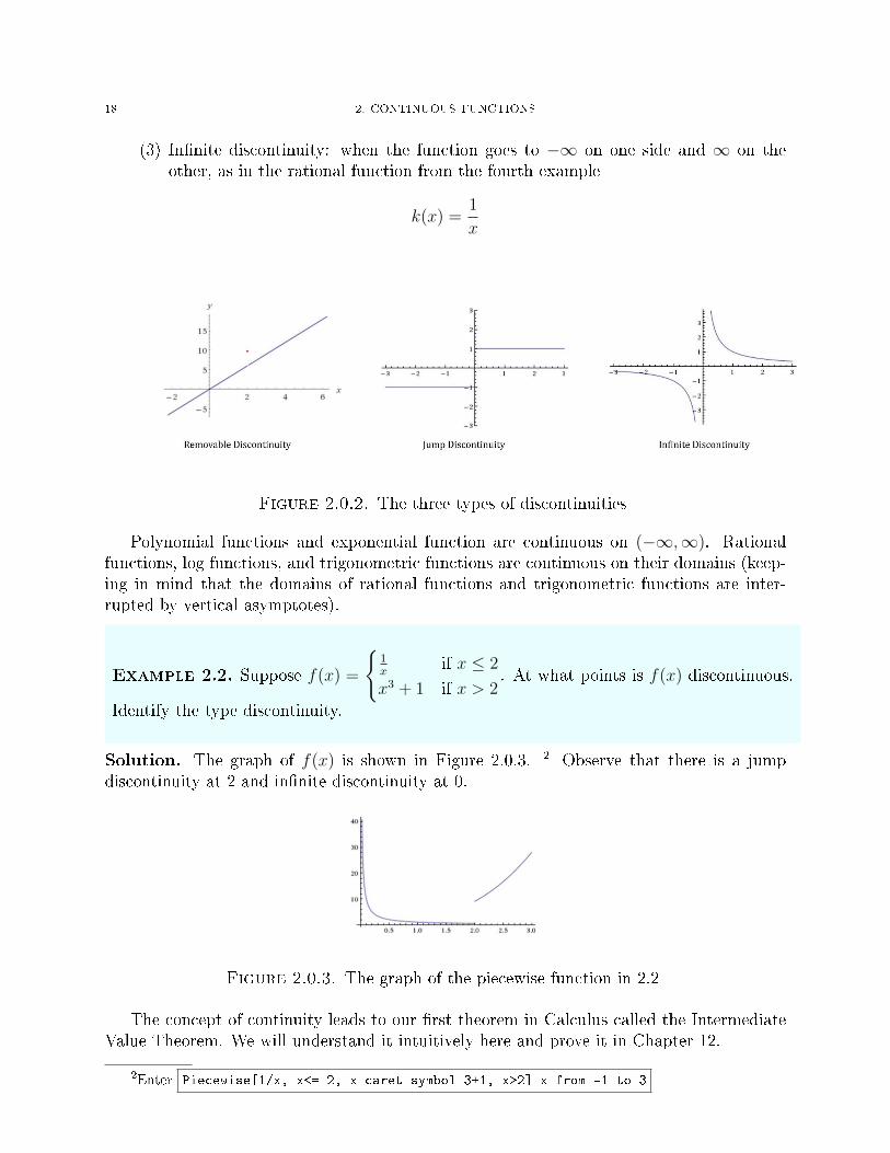
There are three types of discontinuity (see Figure 2.0.2).
(1) Removable discontinuity: when the function has a hole at a point t, but also has alimit at t, as in the piecewise function from the second example
g(x) =
{3x if x 6= 2
8 if x = 2
The function may or may not be de�ned at t.
(2) Jump discontinuity: when the function has a jump at a point t and the limit doesnot exist at t, as in the piecewise function from the third example
h(x) =
{1 if x ≥ 0
−1 if x < 0
1Enter this function in wolframalpha.com as f(x)=sqrt(x) x from 0 to 5 .
18 2. CONTINUOUS FUNCTIONS
(3) In�nite discontinuity: when the function goes to −∞ on one side and ∞ on theother, as in the rational function from the fourth example
k(x) =1
x
Figure 2.0.2. The three types of discontinuities
Polynomial functions and exponential function are continuous on (−∞,∞). Rationalfunctions, log functions, and trigonometric functions are continuous on their domains (keep-ing in mind that the domains of rational functions and trigonometric functions are inter-rupted by vertical asymptotes).
Example 2.2. Suppose f(x) =
{1x
if x ≤ 2
x3 + 1 if x > 2. At what points is f(x) discontinuous.
Identify the type discontinuity.
Solution. The graph of f(x) is shown in Figure 2.0.3. 2 Observe that there is a jumpdiscontinuity at 2 and in�nite discontinuity at 0.
Figure 2.0.3. The graph of the piecewise function in 2.2
The concept of continuity leads to our �rst theorem in Calculus called the IntermediateValue Theorem. We will understand it intuitively here and prove it in Chapter 12.
2Enter Piecewise[1/x, x<= 2, x caret symbol 3+1, x>2] x from -1 to 3

2. CONTINUOUS FUNCTIONS 19
Theorem 2.3. (Intermediate Value theorem) Suppose f is a real-valued function thatis continuous on [a, b] and suppose w is a number such that f(a) ≤ w ≤ f(b). Then, thereexists c ∈ [a, b] such that f(c) = w.
According to the theorem, when the function is continuous, we can choose any numberw between f(a) and f(b) on the y-axis and corresponding to that number w there exists anumber c between a and b on the x-axis such that f(c) = w (See Figure 2.0.4). The theoremdoes not tell us how to �nd the number c, just that there exists such a number. Such resultsare called Existence Theorems. At this stage it is enough to understand the proof of theIntermediate Value Theorem intuitively. The proof is in Chapter 12.
Figure 2.0.4. Picture for Theorem 2.3
The converse is not true. For example, consider the function:
f(x) =
{sin 1
xx 6= 0
0 x = 0
For any interval [a, b] containing 0, f(x) takes on every value between f(a) and f(b)somewhere in [a, b]. But f is not continuous at 0, because limx→0 f(x) does not exist.
As a corollary we obtain the following result whose proof is easy. A root of a function fis a number c such that f(c) = 0. Roots are also called zeros of the function.
Corollary 2.4. (Bolzano's Theorem) Suppose f is a function that is continuous on [a, b]and suppose f(a) and f(b) have opposite signs. Then there exists a root of f in [a, b].
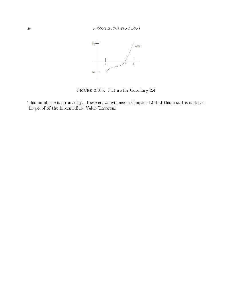
According to the corollary, if f(a) is negative and f(b) is positive and we can draw thefunction without lifting pencil from paper, then at some point the pencil will cross the x-axis(See Figure 2.0.5). That is precisely where a root or zero of the function occurs.
The proof of the above result follows easily from the Intermediate Value Theorem. Sincef is continuous and f(a) and f(b) have opposite signs, the number 0 lies between f(a) andf(b). By the Intermediate Value Theorem, there is a number c in [a, b] such that f(c) = 0.
20 2. CONTINUOUS FUNCTIONS
Figure 2.0.5. Picture for Corollary 2.4
This number c is a root of f . However, we will see in Chapter 12 that this result is a step inthe proof of the Intermediate Value Theorem.
2. CONTINUOUS FUNCTIONS 21
We will end this chapter with an excerpt from Bertrand Russell's essay �Mathematicsand the Metaphysicians,� 3 Historically, limits and continuity came after the discovery ofCalculus, while mathematicians were trying to make Calculus rigorous. Subsequently, theyare presented �rst for pedagogical reasons, so concepts follow in logical order. Unfortunatelythis has the e�ect of discouraging students because limits is harder to grasp than derivativesand integrals. Moreover, the presentation of limits in many textbooks is made unnecessarilyhard by dwelling on formality. Those who �nd limits challenging should �nd it reassuring toknow that limits were hard for mathematicians too.
Calculus required continuity, and continuity was supposed to require thein�nitely little; but nobody could discover what the in�nitely little mightbe. It was plainly not quite zero, because a su�ciently large number ofin�nitesimals, added together, were seen to make up a �nite whole. Butnobody could point out any fraction which was not zero, and yet not �-nite. Thus there was a deadlock. But at last Weierstrass discovered thatthe in�nitesimal was not needed at all, and that everything could be ac-complished without it. Thus there was no longer any need to suppose thatthere was such a thing. ...
The banishment of the in�nitesimal has all sorts of odd consequences, towhich one has to become gradually accustomed. For example, there is nosuch thing as the next moment. The interval between one moment andthe next would have to be in�nitesimal, since, if we take two momentswith a �nite interval between them, there are always other moments in theinterval. Thus if there are to be no in�nitesimals, no two moments arequite con- secutive, but there are always other moments between any two.Hence there must be an in�nite number of moments between any two ;because if there were a �nite number one would be nearest the �rst of thetwo moments, and therefore next to it.
3Bertrand Russell's book of essays titled Mysticism and Logic is available online athttps://archive.org/details/mysticismlogicot00russ. This particular essay begins on page 74.

CHAPTER 3
Techniques for Finding Limits
In the previous chapter we found limits visually, but we also saw that it is not always theeasiest way nor is it always reliable. In this chapter we learn some techniques for �nding limitsbeginning with the limit rules and formulas. The proofs require the formal epsilon-delta de�-nition of limits. They are given in Chapter 12. The distinction between a forumula and a ruleis minor. A formula applies to a speci�c function and a rule applies to any real-valued func-
tion.
Theorem 3.1. (Limit Formulas) Let a and c be real numbers and n be a naturalnumber.
(1) limx→a
c = c
(2) limx→a
x = a
(3) limx→a
xn = an
(4) limx→a
n√x = n√a
Theorem 3.2. (Limit Rules) Let f(x) and g(x) be two real-valued functions, let a be areal number, and let n be a natural number.
(1) limx→a
[f(x)± g(x)] = limx→a
f(x)± limx→a
g(x)]
(2) limx→a
f(x)g(x) = limx→a
f(x) limx→a
g(x)
(3) limx→a
f(x)g(x)
=limx→a
f(x)
limx→a
g(x)
(4) limx→a
[f(x)]n = [limx→a
f(x)]n
(5) limx→a
n√f(x) = n
√limx→a
f(x), where if n is even, then is a positive natural number
(otherwise we get complex numbers).
For example, using these Formulas (1) and (2) and Rules (1) and (2) we can show that
limx→8
2x+ 5 = limx→8
2x+ limx→8
5 = limx→8
2 limx→8
x+ limx→8
5 = 2x+ 8
22

3. TECHNIQUES FOR FINDING LIMITS 23
But this sort of tedious applications of the rules and formulas is not how we will approachlimit problems. For this example, it makes sense to use the fact that a linear function is acontinuous function. Recall that we de�ned a continuous function as a function f(x) withthe property that lim
x→af(x) = f(a). So for continuous functions �nding the limit at a point a
amounts to �nding the value of the function at a (assuming a is in the domain). Functionslike polynomial functions, rational functions, radical functions, exponential functions, andlog functions are continuous on their domains. We will use this feature to obtain limits.
Example 3.3. The following functions are continuous on their domains. Use this fact to�nd the limits.
(1) limx→1
x5 + 2x3 − 3x2 + 4x− 5
(2) limx→3
2x2+x−5x−1
(3) limx→−2
3x − 5
(4) limx→−2
(3x − 1)2
(5) limx→16
√x+ 5
(6) limx→−27
3√x+ 1
Solutions.
(1) limx→1
x5 + 2x3 − 3x2 + 4x− 5 = 1 + 2− 3 + 4− 5 = −1
(2) limx→3
2x2+x−5x−1 = 2(32)+3−5
3−1 = 162
= 8
(3) limx→−2
3x − 5 = 3−2 − 5 = 19− 5 = −44
9
(4) limx→−2
(3x − 1)2 = (3−2 − 1)2 = (19− 1)2 = (−8
9)2 = 64
81
(5) limx→16
√x+ 5 = lim
x→16
√16 + 5 = 4 + 5 = 9
(6) limx→−27
3√x+ 1 = lim
x→−273√−27 + 1 = −3 + 1 = −2
It isn't hard to use a visual understanding of limits for these functions, but using the notionof continuous functions is much more elegant. This is a short list of a large number oflimit problems that can be solved simply by recognizing that the function is continuous onits domain (and the point a is in the domain). Pay careful attention to rational functionswhich are continuous only on their domains. The roots of the denominator are not in the

24 3. TECHNIQUES FOR FINDING LIMITS
domain. This is where the vertical asymptotes occur. For example, since the domain off(x) = 2x2+x−5
x−1 is all real numbers except 1, the function is continuous everywhere else. 1
Rational functions can have holes in them that are hidden at �rst glance as in the nextexample. In fact, when �nding the limit of a rational function we should �rst check for holesby checking if we get 0
0. Later on, after we study derivatives we will learn a method called
L'Hopital's rule that will work in all situations that give 00. But some rational functions can
be handled quite easily without a fancier technqiue.
Example 3.4. Find limx→1
x2−1x−1 .
Solution. Observe that 1 is a root of the denominator. Check to see if it is also a root ofthe numerator giving the 0
0form.
x2 − 1
x− 1=
0
0.
Thus we must �rst factor out (x− 1) and get
limx→1
x2 − 1
x− 1= lim
x→1
(x− 1)(x+ 1)
x− 1= x+ 1 = 1 + 1 = 2.
�
Note that we can cancel (x− 1) from numerator and denominator because we are saying xtends to 1. We are not saying x = 1. The graph of f(x) = x2−1
x−1 is the straight line y = x+ 1with a hole at 1.
How would we tackle a limit problem involving a rational function where the denominatoris a high degree polynomial? For example, consider the function f(x) = x3−x2+x+5
x7+x4−x3+3x2−4 wherefactoring the denominator to �nd the zeros would be di�cult, to say the least, and possiblyoutside the scope of a Calculus course if the Rational Root Test does not work. Even if theRational Root Test does work it would be unbearably tedious to solve a 7th degree equation.
Example 3.5. Find limx→2
x3−x2+x+5x7+x4−x3+3x2−4 .
Solution. Check to con�rm that 2 is not a root of the polynomial in the denominatorx7 + x4− x3 + 3x2− 4. Plugging x = 2 in it gives 27 + 24− 23 + 3(2)2− 4 = 192. So 2 is nota root of the denominator, and therefore in the domain of the rational function. Now theproblem is just like the previous ones.
limx→2
x3 − x2 + x+ 5
x7 + x4 − x3 + 3x2 − 5=
23 − 22 + 2 + 5
27 + 24 − 23 + 3(2)2 − 4=
11
192
�
1The rest of this chapter may be omitted by students taking a �Survey of Calculus� course
3. TECHNIQUES FOR FINDING LIMITS 25
Let's do the same problem again taking the limit value as 1 instead of 2. So the problemis to �nd
limx→1
x3 − x2 + x+ 5
x7 + x4 − x3 + 3x2 − 4.
Observe that
x3 − x2 + x+ 5
x7 + x4 − x3 + 3x2 − 4=
13 − 12 + 1 + 5
(1)7 + (1)4 − (1)3 + 3(1)2 − 4=
6
0.
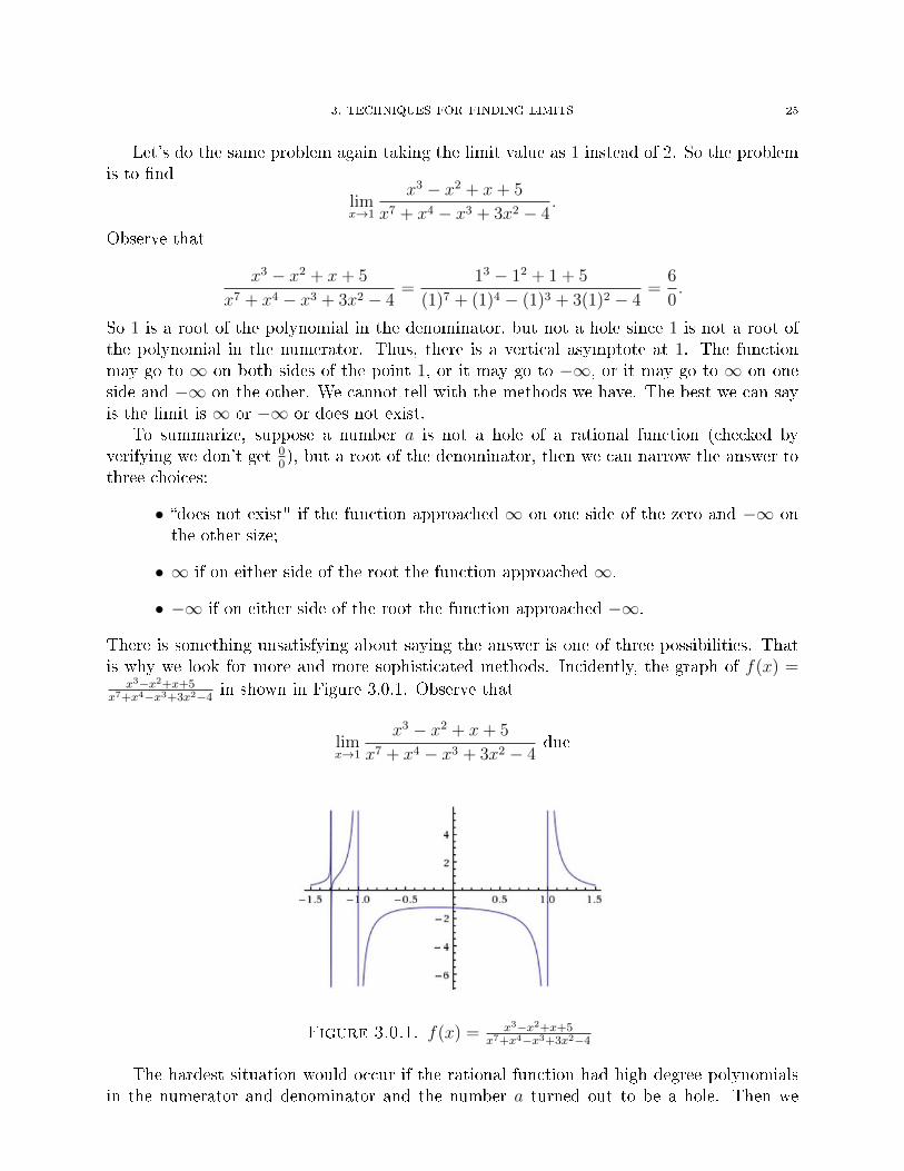
So 1 is a root of the polynomial in the denominator, but not a hole since 1 is not a root ofthe polynomial in the numerator. Thus, there is a vertical asymptote at 1. The functionmay go to ∞ on both sides of the point 1, or it may go to −∞, or it may go to ∞ on oneside and −∞ on the other. We cannot tell with the methods we have. The best we can sayis the limit is ∞ or −∞ or does not exist.
To summarize, suppose a number a is not a hole of a rational function (checked byverifying we don't get 0
0), but a root of the denominator, then we can narrow the answer to
three choices:
• �does not exist" if the function approached ∞ on one side of the zero and −∞ onthe other size;
• ∞ if on either side of the root the function approached ∞.
• −∞ if on either side of the root the function approached −∞.
There is something unsatisfying about saying the answer is one of three possibilities. Thatis why we look for more and more sophisticated methods. Incidently, the graph of f(x) =
x3−x2+x+5x7+x4−x3+3x2−4 in shown in Figure 3.0.1. Observe that
limx→1
x3 − x2 + x+ 5
x7 + x4 − x3 + 3x2 − 4dne
Figure 3.0.1. f(x) = x3−x2+x+5x7+x4−x3+3x2−4
The hardest situation would occur if the rational function had high degree polynomialsin the numerator and denominator and the number a turned out to be a hole. Then we
26 3. TECHNIQUES FOR FINDING LIMITS
would have to divide the numerator and denominator by (x − a), cancel out the commonfactor (x− a) and repeat all over again. Fortunately, later on we will learn L'Hopital's Rulethat can solve the problem in less than a minute.
The second technique we study is an algebraic way of handling rational functions withradicals without graphing them. This technique is called �Rationalizing the denominator."To implement it multiply numerator and denominator by the rational conjugate.
Example 3.6. Find limx→0
√x2+9−3x2
.
Solution.
limx→0
√x2 + 9− 3
x2= lim
x→0
√x2 + 9− 3
x2×√x2 + 9 + 3√x2 + 9 + 3
= limx→0
x2 + 9− 9
x2√
(x2 + 9) + 3
= limx→0
x2
x2√
(x2 + 9) + 3
= limx→0
1√(x2 + 9) + 3
=1
6
Notice how algebraic operations can simplify the function so that plugging 0 in it does notcause problems in the denominator. This method will not work for all radical expressions,but when it works it works well.
The third technique is a more sophisticated method that depends on a theorem. Theproof of this theorem is given in Chapter 12.
Theorem 3.7. (Sandwich Theorem) suppose f(x) ≤ h(x) ≤ g(x), for every x in an openinterval containing a point a except possibly at a. If lim
x→af(x) = lim
x→ag(x) = L, then
limx→a
h(x) = L.
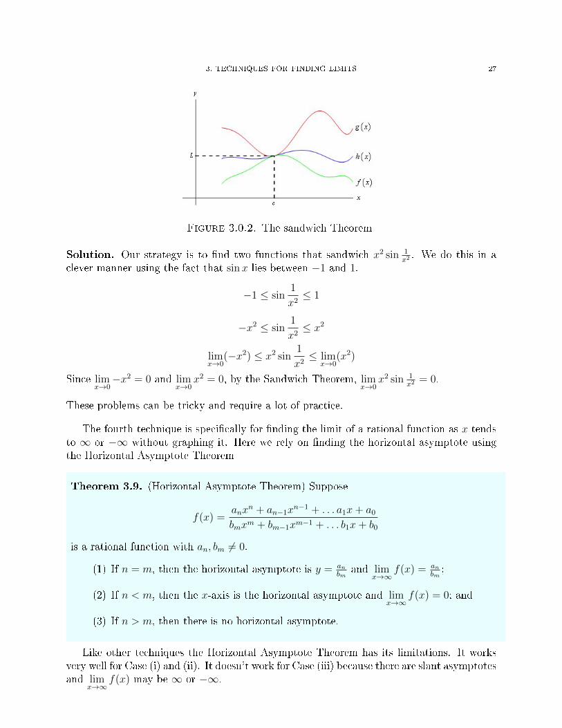
See Figure 3.0.2 to understand this result intuitively. Since f(x) ≤ h(x) ≤ g(x), the limitgets trapped between lim
x→af(x) and lim
x→ag(x) and since both are L, it follows that lim
x→ah(x) is
also L. Hence the name Sandwich Theorem.
Example 3.8. Find limx→0
x2 sin 1x2.
3. TECHNIQUES FOR FINDING LIMITS 27
Figure 3.0.2. The sandwich Theorem
Solution. Our strategy is to �nd two functions that sandwich x2 sin 1x2. We do this in a
clever manner using the fact that sinx lies between −1 and 1.
−1 ≤ sin1
x2≤ 1
−x2 ≤ sin1
x2≤ x2
limx→0
(−x2) ≤ x2 sin1
x2≤ lim
x→0(x2)
Since limx→0−x2 = 0 and lim
x→0x2 = 0, by the Sandwich Theorem, lim
x→0x2 sin 1
x2= 0.
These problems can be tricky and require a lot of practice.
The fourth technique is speci�cally for �nding the limit of a rational function as x tendsto ∞ or −∞ without graphing it. Here we rely on �nding the horizontal asymptote usingthe Horizontal Asymptote Theorem
Theorem 3.9. (Horizontal Asymptote Theorem) Suppose
f(x) =anx
n + an−1xn−1 + . . . a1x+ a0
bmxm + bm−1xm−1 + . . . b1x+ b0
is a rational function with an, bm 6= 0.
(1) If n = m, then the horizontal asymptote is y = anbm
and limx→∞
f(x) = anbm;
(2) If n < m, then the x-axis is the horizontal asymptote and limx→∞
f(x) = 0; and
(3) If n > m, then there is no horizontal asymptote.
Like other techniques the Horizontal Asymptote Theorem has its limitations. It worksvery well for Case (i) and (ii). It doesn't work for Case (iii) because there are slant asymptotesand lim
x→∞f(x) may be ∞ or −∞.

28 3. TECHNIQUES FOR FINDING LIMITS
Example 3.10. Find the limits.
(1) limx→∞
3x+45x+7
(2) limx→∞
2x2−53x2+x+5
(3) limx→∞
x2−1x2+1
(4) limx→∞
x2+3x+13x4−1
Solutions.
(1) limx→∞
3x+45x+7
= 34
Note that, since the degree of the numerator is the same as the degree of the denom-inator, we can give the answer instantly using the Horizontal Asymptote Theorem.
(2) limx→∞
2x2−53x2+x+5
= 23
(3) limx→∞
x2−1x2+1
= 1
(4) limx→∞
x2+3x+13x4−1 = 0
Note that since the degree of the numerator is less than the degree of the denomi-nator, by the Horizontal Asymptote Theorem, the x-axis, i.e. the line y = 0, is thehorizontal asymptote.
�
The ease of answering these limit problems makes the Horizontal Asymptote Theorem apowerful technique and worth understanding thoroughly. So what exactly is going on here?Let's take another look at the �rst example
limx→∞
3x+ 4
5x+ 7
Divide numerator and denominator by the highest power of x, in this case just x, to get
3. TECHNIQUES FOR FINDING LIMITS 29
limx→∞
3x+ 4
5x+ 7= lim
x→∞
3x+4x
5x+7x
= limx→∞
3xx
+ 4x
5xx
+ 7x
= limx→∞
3 + 4x
5 + 7x
=limx→∞
3 + limx→∞
4x
limx→∞
5 + limx→∞
7x
=3 + 0
5 + 0
=3
5
Consider the fourth example again
limx→∞
x2 + 3x+ 1
3x4 − 1
Divide numerator and denominator by the highest power of x, in this case x4, to get
limx→∞
x2 + 3x+ 1
x4 − 1= lim
x→∞
x2
x4+ 3x
x4+ 1
x4
x4
x4− 1
x4
= limx→∞
1x2
+ 3x3
+ 1x4
3− 1x4
=limx→∞
1x2
+ limx→∞
3x3
+ limx→∞
1x4
limx→∞
3− limx→∞
1x4
=0
3= 0
These are all the steps where we carefully apply the limit rules and get the answer. Weare expected to know the graph of y = 1
xand the fact that lim
x→∞1x
= 0. We will prove this
formally in Chapter 12.
Next we will give a proof of the �rst two cases of the Horizontal Asymptote Theorem.The proofs are just like the steps in the above two problems, except that we have arbitrarypolynomials in the numerator and denominator instead of speci�c ones. The third caserequires the formal de�nition of limits and appears in Chapter 12.

30 3. TECHNIQUES FOR FINDING LIMITS
Partial Proof of the Horizontal Asymptote Theorem.
(1) Suppose n = m.
f(x) =anx
n + an−1xn−1 + . . . a1x+ a0
bnxn + bn−1xn−1 + . . . b1x+ b0.
Since the highest power of x is n, divide numerator and denominator by xn to get
f(x) =anxn
xn+ an−1xn−1
xn+ . . . a1x
xn+ a0
xn
bnxn
xn+ bn−1xn−1
xn+ . . . b1x
xn+ b0
xn
Since limit of a quotient is quotient of a limit and limit of a sum is sum of limits,we can take limit of each term. As x tends to ∞ all the terms tend to 0 exceptthe �rst term in the numerator and the �rst term in the denominator where the xn
cancel out. Solimx→∞
f(x) = limx→∞
anbn
=anbn.
(2) Suppose n < m. Then
f(x) =anx
n + an−1xn−1 + . . . a1x+ a0
bmxm + bm−1xm−1 + . . . b1x+ b0.
Since the highest power of x is m, divide numerator and denominator by xm to get
f(x) =anxn
xm+ an−1xn−1
xm+ . . . a1x
xm+ a0
xm
bmxm
xm+ bm−1xm−1
xm+ . . . b1x
xm+ b0
xm
Since limit of a quotient is quotient of a limit and limit of a sum is sum of limits,we can take limit of each term. As x tends to ∞ all the terms tend to 0 except the�rst term in the denominator where the xm cancels out. So
limx→∞
f(x) = limx→∞
0
bm= 0
�
The technique of dividing numerator and denominator by the highest power of x is veryuseful even when the function is not a rational function.
Example 3.11. Find the limits.
(1) limx→∞
√10x2+24x+3

3. TECHNIQUES FOR FINDING LIMITS 31
Solution. Begin by dividing by the highest power of x. Since x2 is under the radical signthe highest power of x is x itself.
limx→∞
√10x2 + 3
4x+ 3= lim
x→∞
√x2(10 + 2
x2)
4x+ 3
= limx→∞
x√
10+ 2x2
x4x+3x
= limx→∞
√10 + 2
x2
4 + 3x
=
√10
4
�
This brings us to the end of Chapter 3. You should think of the techniques for solvinglimits as a set of tools and like any set of tools, the same technique doesn't work for allthe limit problems. With practice it becomes easier to recognize which ones work for whichproblems.
Practice Problems
(1) Find the limits using the limit rules.
a) limx→√2 15
b) limx→−2 x
c) limx→4 3x− 4
d) limx→−2x−54x+3
e) limx→1(−2x+ 5)4
f) limx→−2(3x3 − 2x+ 7)
g) limx→46x−12x−9
h) limx→2x2+x−2(x−2)2
i) limx→−2x3+8x4−16
j) limx→2
1x− 1
2
x−2
k) limx→1
(x2
x−1 −1
x−1
)l) limx→0
4−√x+16x

32 3. TECHNIQUES FOR FINDING LIMITS
m) limx→1x2−x−2x5−1
n) limx→3 x2(3x− 4)(9− x3)
o) limx→5+√x2 − 25 + 3
p) limx→3+
√(x−3)2x−3
(2) Use the Sandwich Theorem to �nd the following limits. Show your work in detail.
a) If 4x− 9 ≤ f(x) ≤ x2 − 4x+ 7 for x ≥ 0, �nd limx→4 f(x).
b) If 2x ≤ g(x) ≤ x4 − x2 + 2 for all x, �nd limx→1 g(x).
c) limx→0
√x3 + x2 sin π
x
d) limx→0 x4 cos 2
x
(3) Find the limit, if it exists, using a technique from this chapter.
a) limx→5−√
5− xb) limx→2
√8− x3
c) limx→13√x3 − 1
d) limx→45
x−4
e) limx→ 52
8(2x+5)3
f) limx→∞1
x(x−3)2
g) limx→∞−x3+2x2x2−3
h) limx→−∞2−x2x+3
i) limx→−∞4x−3√x2−1
j) limx→∞2x2
x2−x−2
k) limx→∞5x2−3x+12x2+4x−7
l) limx→∞3x
(x+8)2
m) limx→−∞4−7x2+3x
n) limx→−∞2x2−34x3+5x
o) limx→∞3
√8+x2
x(x+1)

CHAPTER 4
What is a Derivative?
German mathematician Gottfried Wilhelm von Leibniz (1646 - 1716) and British mathemati-cian Sir Isaac Newton (1642 - 1726) get the credit for discovering Calculus. Poet AlexanderPope beautifully captures the greatness of this discovery as follows:
Nature and nature's laws lay hid in night:
God said, �Let Newton be!� and all was light.
Newton and Leibniz discovered Calculus independently and the ensuing �ght for credit makesfor interesting reading (see Figure 4.0.1). 1
Figure 4.0.1. The fathers of Calculus
Suppose we have to drive from Brooklyn, NY to Niagara Falls, NY. Google shows thatthe distance is 412 miles and it takes 7 hours. Using the well-known formula
distance = speed× time
we may conclude that our speed is
speed =distance
time=
412
7= 58.86 miles/hour.
1Images taken from Wikipedia. This portrait of a 46 year old Newton was painted in 1689 by famouspotrait artist Godfrey Kneller. Leibniz's portrait appears in the Public Library of Hannover.
33

34 4. WHAT IS A DERIVATIVE?
Does this mean we were driving exactly 58.86 miles per hour the entire way? A glanceat the odometer shows that the needle is constantly moving. So the �average speed� maybe 58.86 miles per hour over the entire 7 hour trip, but �instantaneous speed� is changingconstantly. And what exactly is an instant? Is it 1 minute, 1 second, 0.1 second, or smaller?We represent an instant as a point on the number line. A point is an in�nitessimily small0-dimensional entity. In other words it has no length, breadth, or height. Note that wecannot actually draw a point that has no length, breadth, or height, no matter how �ne wemake it, so we must imagine that the dot on the page has no dimension.
There is an inherent di�culty capturing the concept of motion at an instant. Arguably atan instant there is no motion because if we take a photo of a moving car we will get a pictureof a motionless car. Zeno of Elea (c. 490 BC - 430 BC) was grappling with these conceptsin the 3rd century BC. He was a member of the Eleatic School founded by the philosopherParmenides (c. 515 BC - 460 BC), who is famous for his poem on the impermeance ofchange. 2
Mortals have made up their minds to name two forms, one of which theyshould not name, and that is where they go astray from the truth. Theyhave distinguished them as opposite in form, and have assigned to themmarks distinct from one another. To the one they allot the �re of heaven,gentle, very light, in every direction the same as itself, but not the same asthe other. The other is just the opposite to it, dark night, a compact andheavy body. Of these I tell you the whole arrangement as it seems likely;for so no thought of mortals will ever outstrip you.
Zeno wrote a set of three paradoxes that appear in Aristotle's Physics. We will dicuss the�rst two later; the third is relevant at this junction.
If everything when it occupies an equal space is at rest, and if that which isin locomotion is always occupying such a space at any moment, the �yingarrow is therefore motionless.
In this ��ying arrow is motionless� paradox, Zeno is trying to make arguments in support ofParmenides's doctrine that our senses cannot be trusted; change, and motion in particular,is just an illusion. Zeno was arguing that an object �occupies� a small space at an instant,and is therefore motionless at an instant. Aristotle rejected Zeno's reasoning in no uncertainterms.
Zeno's reasoning, however, is fallacious, when he says that if everythingwhen it occupies an equal space is at rest, and if that which is in locomo-tion is always occupying such a space at any moment, the �ying arrow is
2 Parmenides wrote a poem On Nature explaining his philosophy. The �rst part calledProem is the introduction, the second called The Way of Truth gives his view on reality, andthe third called The Way of Opinion explains the deceptive nature of reality as it appears tous. The complete version has not been found, but other philosophers were greatly in�uencedby it and wrote extensively about it. It somewhat mind-bending to read, the poem is fullof interesting philosophical ideas. See http://www.mycrandall.ca/courses/grphil/parmenides.htm andhttp://plato.stanford.edu/entries/parmenides/ for more information.

4. WHAT IS A DERIVATIVE? 35
therefore motionless. This is false, for time is not composed of indivisiblemoments any more than any other magnitude is composed of indivisibles.
However, Zeno has the last laugh, and if Aristotle had not so resolutely rejected his attemptsto understand motion, perhaps Calculus might have been invented earlier.
The fresco in Figure 4.0.2 shows Plato and Aristotle in the center under the arch, Euclidon the right holding a compass, Zeno on the far left, Phythagorous reading a book, andParmenides in an orange robe looking down at him. It was drawn in 1511 by the famouspainter Raphael in the Sistine Chapel at the Vatican, Italy 3
Figure 4.0.2. School Of Athens
There is some paradox in trying to quantify motion at an instant because when the focusis on a single moment the motion stops. Sir Issac Newton's and independently GottfriedWilhelm Leibniz's brilliant approach to motion was to stop looking for a way to de�ne motionat an instant, but instead to look at smaller and smaller intervals containing that instant.Consider Figure 4.0.3 that gives the distance the car every hour for the 7 hour trip fromBrooklyn to Niagara Falls. The overall distance covered is 412 hours in 7 hours. As notedearlier the average speed is 412
7= 58.86 miles per hour. The graph on the right of the table
is a plot of time on the x-axis and distance on the y-axis.Consider a di�erent scenario: throw an apple straight up in the air. Suppose it hits
the ground in 7 seconds. The table in Figure 4.0.4 gives the height of the apple at eachsecond. The graph next to it is the graph of time versus height of the orange (not to beconfused with the path the apple takes). Observe that the apple starts at 6 feet assuming
3 Image taken from Wikipedia

36 4. WHAT IS A DERIVATIVE?
Figure 4.0.3. Distance traveled by a car
the person throwing the apple up is 6 feet tall. It reaches a highest point of 50 feet afterwhich it falls back down reaching the ground in 7 seconds. What now is the average heightsince technically at the end the apple has height 0? The speed in this scenario has direction.When the apple is going up the speed is positive and when it is coming down the speed isnegative. Speed with direction (positive or negative) is called velocity. From now on wewill use the term velocity.
Figure 4.0.4. Height of an apple thrown up
Instead of trying to de�ne velocity at an instant of time, consider a small interval (a, b)around an instant t and de�ne average velocity as follows:
Average velocity at t =change in distancechange in time
=f(b)− f(a)
b− a...................(1)
Observe that f(b)−f(a)b−a is the slope of the line that passes through the points (a, f(a)) and
(b, f(b)). It is called the secant line. If we let
b− a = h,
thenb = a+ h.
We can write (1) as
Average velocity at t =f(a+ h)− f(a)
h..................(2)
As the interval shrinks, in other words as h tends to 0, the point a+h merges with the pointa and we can write (2) as
Instantaneous velocity at a = limh→0
f(a+ h)− f(a)
h
4. WHAT IS A DERIVATIVE? 37
This is the derivative at a. The secant line becomes the tangent line at a.
There is nothing special about distance, time, and velocity (other than this is how it allstarted). We can de�ne this concept for any function. Let f be any continuous functionde�ned on an open interval (a, b). Consider the secant line joining points (a, f(a)) and(b, f(b)). The slope of this secant line is
slope =f(b)− f(a)
b− a.
Let b = a+ h and write the interval as (a, a+ h) so the slope can be written as
slope =f(a+ h)− f(a)
h.
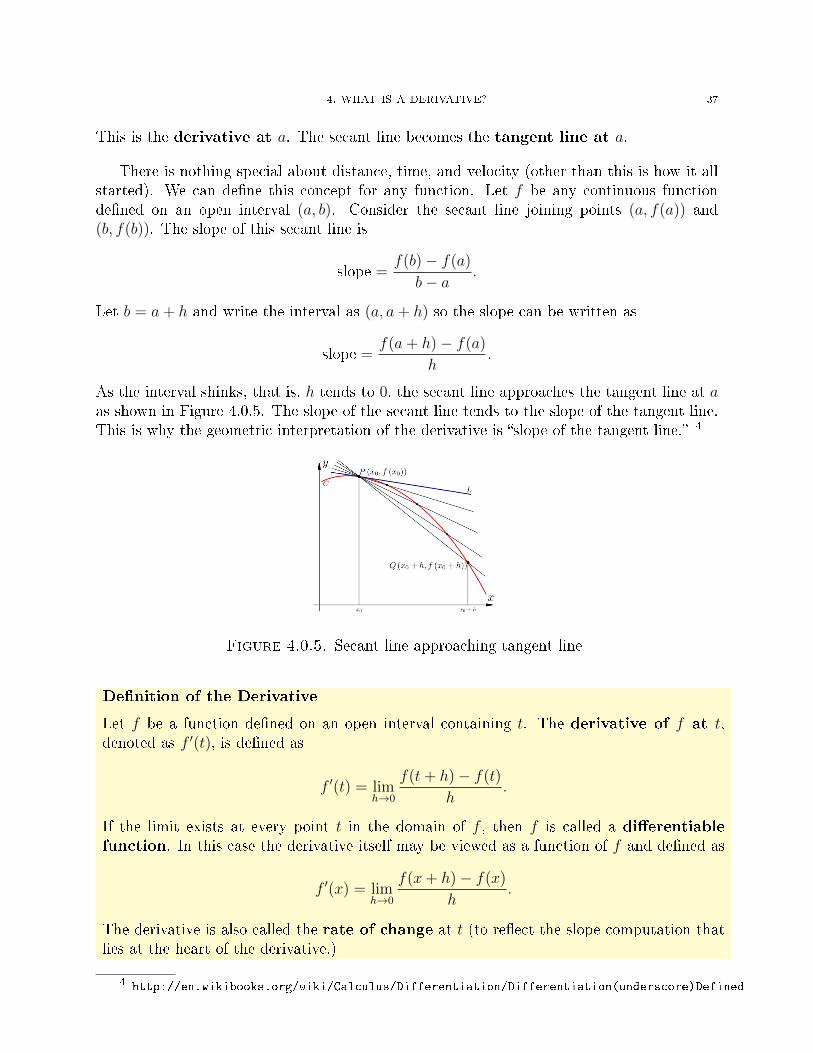
As the interval shinks, that is, h tends to 0, the secant line approaches the tangent line at aas shown in Figure 4.0.5. The slope of the secant line tends to the slope of the tangent line.This is why the geometric interpretation of the derivative is �slope of the tangent line.� 4
Figure 4.0.5. Secant line approaching tangent line
De�nition of the Derivative
Let f be a function de�ned on an open interval containing t. The derivative of f at t,denoted as f ′(t), is de�ned as
f ′(t) = limh→0
f(t+ h)− f(t)
h.
If the limit exists at every point t in the domain of f , then f is called a di�erentiablefunction. In this case the derivative itself may be viewed as a function of f and de�ned as
f ′(x) = limh→0
f(x+ h)− f(x)
h.
The derivative is also called the rate of change at t (to re�ect the slope computation thatlies at the heart of the derivative.)
4 http://en.wikibooks.org/wiki/Calculus/Differentiation/Differentiation(underscore)Defined
38 4. WHAT IS A DERIVATIVE?
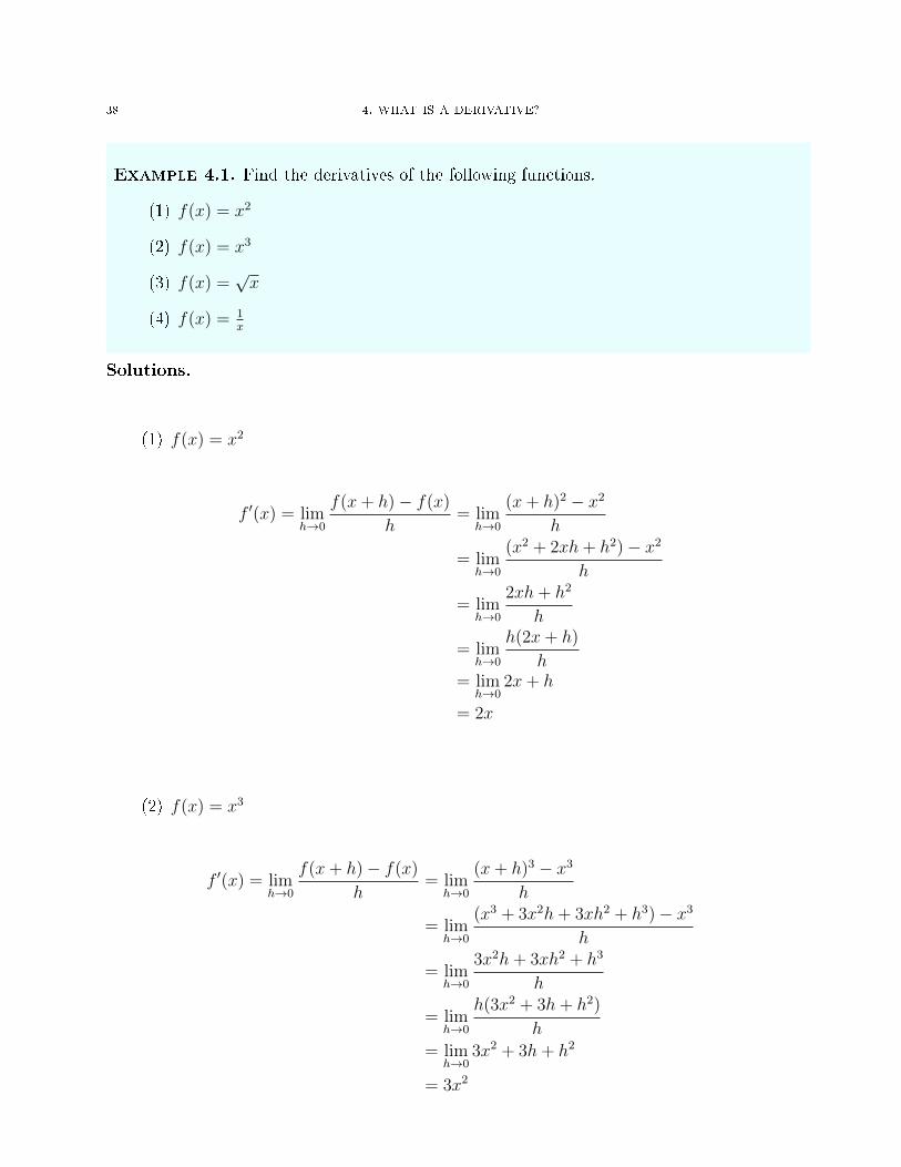
Example 4.1. Find the derivatives of the following functions.
(1) f(x) = x2
(2) f(x) = x3
(3) f(x) =√x
(4) f(x) = 1x
Solutions.
(1) f(x) = x2
f ′(x) = limh→0
f(x+ h)− f(x)
h= lim
h→0
(x+ h)2 − x2
h
= limh→0
(x2 + 2xh+ h2)− x2
h
= limh→0
2xh+ h2
h
= limh→0
h(2x+ h)
h= lim
h→02x+ h
= 2x
(2) f(x) = x3
f ′(x) = limh→0
f(x+ h)− f(x)
h= lim
h→0
(x+ h)3 − x3
h
= limh→0
(x3 + 3x2h+ 3xh2 + h3)− x3
h
= limh→0
3x2h+ 3xh2 + h3
h
= limh→0
h(3x2 + 3h+ h2)
h
= limh→0
3x2 + 3h+ h2
= 3x2

4. WHAT IS A DERIVATIVE? 39
(3) f(x) =√x
f ′(x) = limh→0
f(x+ h)− f(x)
h= lim
h→0
√x+ h−
√x
h
= limh→0
√x+ h−
√x
h×√x+ h+
√x√
x+ h+√x
= limh→0
x+ h− xh(√x+ h+
√x)
= limh→0
h
h(√x+ h+
√x)
= limh→0
1√x+ h+
√x
=1
2√x
(4) f(x) = 1x
f ′(x) = limh→0
f(x+ h)− f(x)
h= lim
h→0
1x+h− 1
x
h
= limh→0
x−(x+h)x(x+h)
h
= limh→0
hx(x+h)
h
= limh→0
−hhx(x+ h)
= limh→0
−1
x(x+ h)
= − 1
x2
�
Suppose the function is not known and we just have some data as in Table 4 and weknow that x is the independent variable and y is the dependent variable. Then we cannot�nd the derivative using a formula and we have to adopt a computational approach.
We can compute the slope at each consecutive pairs of points to obtain the approximatederivative at each point. The third row in Table 2 strongly suggests that f ′(2) is in thevicinity of 12. We cannot say for sure it is 12, but we had to make an educated guess wewould say the derivative at 2 is roughly 12.
The above function is in fact f(x) = x3 and we calculated its derivative precisely earlieras f ′(x) = 3x2. Observe that f ′(2) = 3(22) = 12. So there is merit to this computationalapproach. It is very handy for real-world data that does not �t into a neat well-known

40 4. WHAT IS A DERIVATIVE?
x y = f(x)1.98 7.7623921.99 7.880599
2 82.01 8.1206012.02 8.242408
Table 1. Data on two related variables x and y
x y y2−y1x2−x1
1.98 7.7623921.99 7.880599 7.880599−7.762392
1.99−1.98 = 11.8207
2 8 8−7.8805992−1.99 = 11.9401
2.01 8.120601 8.120601−82.01−2 = 12.0601
2.02 8.242408 8.242408−8.1206012.02−2.01 = 12.1807
Table 2. Rate of change of y
functions. For example, house prices or the Standard and Poor 500 index cannot be modeledby any function. But we can certainly calculate the derivative or rate of change just basedon the data. The next example further illustrates the computational approach.
Example 4.2. Find the rate of change of Ph.ds awarded in science and engineering fromthe data shown in Figure 4.0.6. Interpret your results. Repeat the exercise for non-scienceand engineering Ph.ds. 5
Figure 4.0.6. Doctorates awarded: 1998 - 2008
Solution. Observe from Figure 4.0.6 that when the rate of change is negative the graph is
decreasing on the interval and when the rate of change is positive the graph is increasing.

4. WHAT IS A DERIVATIVE? 41
Year Science and engineering y2−y1x2−x1
1998 272741999 25931 -13432000 25966 352001 25529 - 4372002 24608 -9212003 25282 6742004 26274 9922005 27986 17122006 29863 18772007 31800 19372008 32827 1027
Table 3. Rate of change of doctorates awarded
From 2003 to 2007 the rate of change was increasing, but in 2008 the rate of change decreased(even though the number of doctorates awarded is 1027 more than those awarded in 2007).�
Next, we will look at an example where the derivative does not exist. But �rst let's layerin two more terms: the left derivative and the right derivative. We de�ne them in a mannersimilar to left and right limits.
De�nition of Left and Right Derivative
The left derivative of f at t, denoted as f ′−(t) is de�ned as
f ′−(t) = limh→0−
f(t+ h)− f(t)
h.
The right derivative of f at t, denoted as f ′+(t) is de�ned as
f ′+(t) = limh→0+
f(t+ h)− f(t)
h.
If the left and right derivative both exist and are equal then the derivative exists and is equalto the left (and right) derivative.
Calculating left and right derivatives and showing they are unequal is a way of showingthe derivative does not exist.
Example 4.3. Show that the derivative of f(x) = |x| does not exist at 0.

42 4. WHAT IS A DERIVATIVE?
Solution.
f ′(0) = limh→0
f(0 + h)− f(0)
h= lim
h→0
|h| − 0
h
= limh→0
|h|h
The function y = |x|xis the same as the step function
y =
{−1 if x < 0
1 if x > 0
Revisiting its graph shown in Figure 1.0.3 we see that
limx→0
|x|x
dne
since the left and right limits are not the same. Therefore, f ′(0) does not exist. �
Informally, we can recognize points where the derivative does not exist by looking at thegraph of f(x) = |x| itself. See the left graph in Figure 4.0.7. Let us try zooming in near 0(graph on the right in Figure 4.0.7). Observe that the zoomed in graph on the right looksexactly the same as the original graph on the left. In fact, the only indication that theseare not the exact same �gures appears on the x-axis. No matter how much we zoom in thesharp point at 0 will be present in f(x) = |x|.
Figure 4.0.7. f(x) = |x|
Constrast this with the function f(x) = x2 where as you zoom in closer and closer around0 the curve will look like more and more like a straight line. In fact, this goes to the heartof the derivative notion as slope of the tangent line at a point. In a �smooth� curve like anypolynomial function, if you zoom in at a point it will look a straight line. But for a functionlike f(x) = |x| with a sharp point at 0, there is an abrupt change occuring. The function isnot smooth. 6 The next example is another example of a function where the derivative doesnot exist and in this case the reason is quite di�erent.
Example 4.4. Show that the derivative of f(x) = x13 does not exist at 0.
6Smooth is a technical term that means the derivatives of all orders exist. We will discuss it later.
4. WHAT IS A DERIVATIVE? 43
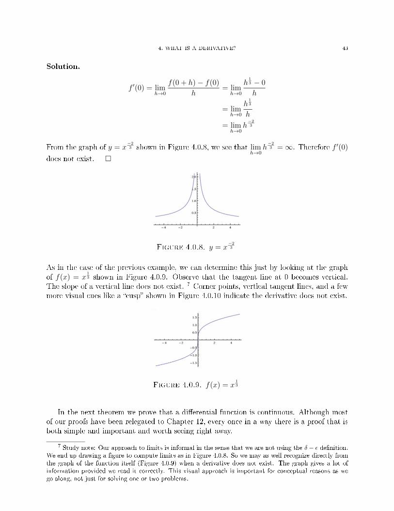
Solution.
f ′(0) = limh→0
f(0 + h)− f(0)
h= lim
h→0
h13 − 0
h
= limh→0
h13
h
= limh→0
h−23
From the graph of y = x−23 shown in Figure 4.0.8, we see that lim
h→0h−23 =∞. Therefore f ′(0)
does not exist. �
Figure 4.0.8. y = x−23
As in the case of the previous example, we can determine this just by looking at the graphof f(x) = x
13 shown in Figure 4.0.9. Observe that the tangent line at 0 becomes vertical.
The slope of a vertical line does not exist. 7 Corner points, vertical tangent lines, and a fewmore visual cues like a �cusp� shown in Figure 4.0.10 indicate the derivative does not exist.
Figure 4.0.9. f(x) = x13
In the next theorem we prove that a di�erential function is continuous. Although mostof our proofs have been relegated to Chapter 12, every once in a way there is a proof that isboth simple and important and worth seeing right away.
7 Study note: Our approach to limits is informal in the sense that we are not using the δ − ε de�nition.We end up drawing a �gure to compute limits as in Figure 4.0.8. So we may as well recognize directly fromthe graph of the function itself (Figure 4.0.9) when a derivative does not exist. The graph gives a lot ofinformation provided we read it correctly. This visual approach is important for conceptual reasons as wego along, not just for solving one or two problems.

44 4. WHAT IS A DERIVATIVE?
Figure 4.0.10. f(x) =3√x2
Theorem 4.5. If a function f is di�erentiable at a, then f is continuous at a.
Proof. To prove that f is continuous at a, we must show that limx→a
f(x) = f(a). Observe
that we can write f(x) algebraically as
f(x) =f(x)− f(a)
x− a(x− a) + f(a)
To see this simplify the right side of the above expression and we get precisely f(x). So
limx→a
f(x) = limx→a
f(x)− f(a)
x− a(x− a) + f(a)
= limx→a
f(x)− f(a)
x− alimx→a
(x− a) + limx→a
f(a)
= f ′(a)(a− a) + f(a)
= f(a)
�
The converse of Theorem 4.5 is not true. We already saw that f(x) = |x| is a functionthat is continuous everywhere, but not di�erentiable at 0. The general thinking amongmathematicians of the 18th century was that a continuous function would have just a fewnon-di�erentiable points. Then German mathematician Karl Weierstrass (1815 - 1897) founda function that was continuous everywhere and di�erentiable nowhere. The function is givenin the format of a power series (which we will study later). It is given by
f(x) =∞∑k=1
ak cos bkπx
where 0 < a < 1 and b is any odd interger such that ab > 3π2
+ 1. A speci�c example of sucha function where a = 1
2, b = 3 and n = 3 is given below and its graph is shown in Figure
4.0.11. 8 The graph on the left of Figure 4.0.11 is a zoomed in version of the graph on the
8Enter this function as f(x) = cos(3*x*pi)/2 + cos(9*x*pi)/4 + cos(27*x*pi)/8.
4. WHAT IS A DERIVATIVE? 45
right.
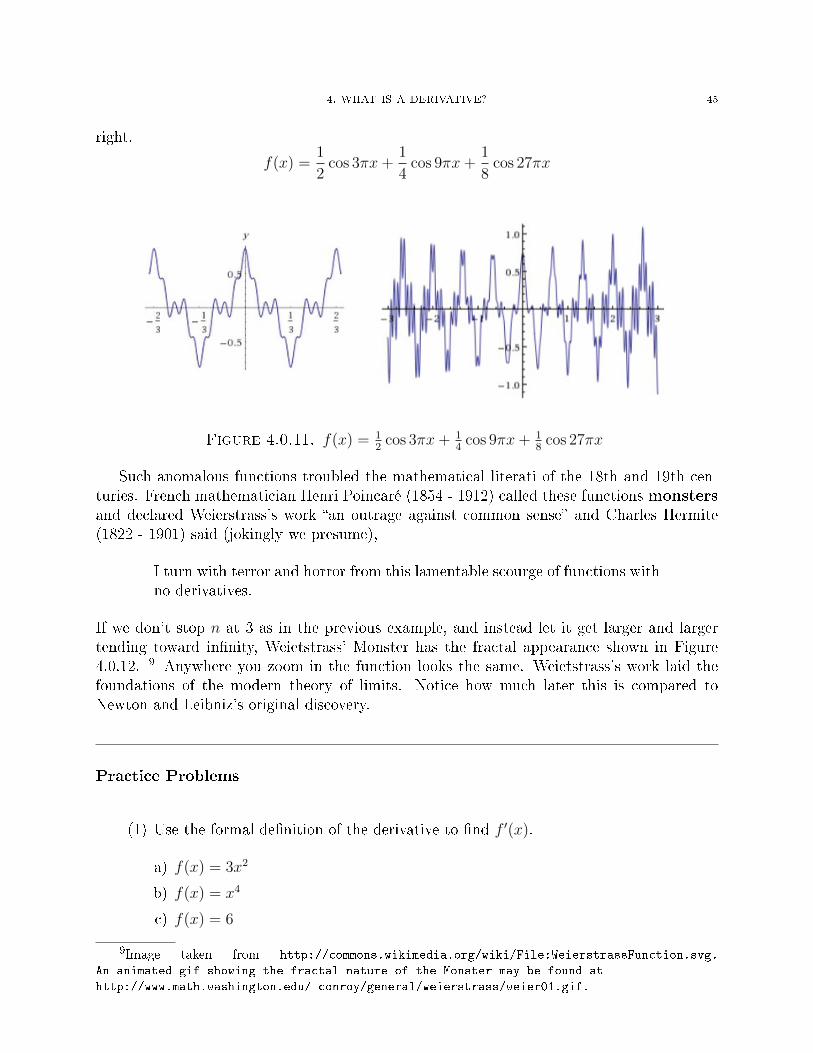
f(x) =1
2cos 3πx+
1
4cos 9πx+
1
8cos 27πx
Figure 4.0.11. f(x) = 12
cos 3πx+ 14
cos 9πx+ 18
cos 27πx
Such anomalous functions troubled the mathematical literati of the 18th and 19th cen-turies. French mathematician Henri Poincaré (1854 - 1912) called these functions monstersand declared Weierstrass's work �an outrage against common sense� and Charles Hermite(1822 - 1901) said (jokingly we presume),
I turn with terror and horror from this lamentable scourge of functions withno derivatives.
If we don't stop n at 3 as in the previous example, and instead let it get larger and largertending toward in�nity, Weietstrass' Monster has the fractal appearance shown in Figure4.0.12. 9 Anywhere you zoom in the function looks the same. Weietstrass's work laid thefoundations of the modern theory of limits. Notice how much later this is compared toNewton and Leibniz's original discovery.
Practice Problems
(1) Use the formal de�nition of the derivative to �nd f ′(x).
a) f(x) = 3x2
b) f(x) = x4
c) f(x) = 6
9Image taken from http://commons.wikimedia.org/wiki/File:WeierstrassFunction.svg.
An animated gif showing the fractal nature of the Monster may be found at
http://www.math.washington.edu/ conroy/general/weierstrass/weier01.gif.

46 4. WHAT IS A DERIVATIVE?
Figure 4.0.12. Weietstrass' Monster
d) f(x) = c, where c is a constant
e) f(x) = x
f) f(x) =√x+ 2
g) f(x) = 1x
h) f(x) = 1x2
i) f(x) = xx+1
j) f(x) = 13x−1
k) f(x) = 12x+1
l) f(x) = 42−3x
m) f(x) =√
3− 6x
(2) Determine where the function is not di�erentiable. Explain your answer by drawinga graph and writing a sentence or two.
a) f(x) = |x|b) f(x) =
√x
c) f(x) = 3√x
d) f(x) = |x− 2|+ 3
e) f(x) =√x+ 5
f) f(x) =√
4− x2
CHAPTER 5
Derivative Rules and Formulas
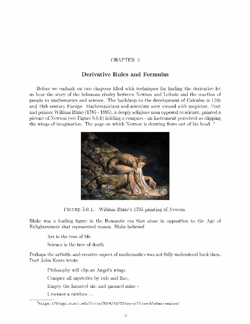
Before we embark on two chapters �lled with techniques for �nding the derivative letus hear the story of the infamous rivalry between Newton and Leibniz and the reaction ofpeople to mathematics and science. The backdrop to the development of Calculus is 17thand 18th century Europe. Mathematicians and scientists were viewed with suspicion. Poetand painter William Blake (1785 - 1895), a deeply religious man opposed to science, painted apicture of Newton (see Figure 5.0.1) holding a compass - an instrument perceived as clippingthe wings of imagination. The page on which Newton is drawing �ows out of his head. 1
Figure 5.0.1. William Blake's 1795 painting of Newton
Blake was a leading �gure in the Romantic era that arose in opposition to the Age ofEnlightenment that represented reason. Blake believed
Art is the tree of life.
Science is the tree of death
Perhaps the artisitic and creative aspect of mathematics was not fully understood back then.Poet John Keats wrote
Philosophy will clip an Angel's wings
Conquer all mysteries by rule and line,
Empty the haunted air, and gnomed mine -
Unweave a rainbow ...
1https://blogs.stsci.edu/livio/2014/10/22/on-william-blakes-newton/
47
48 5. DERIVATIVE RULES AND FORMULAS
and in�uenced Edger Allen Poe to write his famous sonnet �To Science,� 2
Science! true daughter of Old Time thou art!
Who alterest all things with thy peering eyes.
Why preyest thou thus upon the poet's heart,
Vulture, whose wings are dull realities?
One cannot say this era has completely dissapeared. An article in the Guardian titled �Whatmakes some people so suspicious of the �ndings of science?� provides a straightforwardanswer. 3
The scienti�c method leads us to truths that are less than self-evident,often mind-blowing and sometimes hard to swallow. In the early 17thcentury, when Galileo claimed that the Earth spins on its axis and orbitsthe sun, he wasn't just rejecting church doctrine. He was asking peopleto believe something that de�ed common sense - because it sure looks likethe sun's going around the Earth, and you can't feel the Earth spinning.Galileo was put on trial and forced to recant. Two centuries later, CharlesDarwin escaped that fate. But his idea that all life on Earth evolved from aprimordial ancestor and that we humans are distant cousins of apes, whalesand even deep-sea molluscs is still a big ask for a lot of people.
In his lifetime, Newton got into a bitter rivalry with Leibniz that lasted till his death. Thiswas somewhat unusual because Newton was also quite humble judging by his most famousquote, �If I have seen further than others, it is by standing upon the shoulders of giants.�He died feeling robbed of his greatest achievement. In this he appears to have been aidedby well-meaning but trouble-making friends.
In 1695 Newton received a letter from his Oxford mathematician friend JohnWallis, containing news that cast a cloud over the rest of his life. Writing aboutNewton's early mathematical discoveries, Wallis warned him that in Holland�your notions� are known as �Leibniz's Calculus Di�erentialis,� and he urgedNewton to take steps to protect his reputation. At that time the relations betweenNewton and Leibniz were still cordial and mutually respectful. However, Wallis'sletters soon curdled the atmosphere, and initiated the most prolonged, bitter,and damaging of all scienti�c quarrels: the famous (or infamous) Newton-Leibnizpriority controversy over the invention of calculus.
It is now well established that each man developed his own form of calculusindependently of the other, that Newton was �rst by 8 or 10 years but did notpublish his ideas, and that Leibniz's papes of 1684 and 1686 were the earliestpublications on the subject. However, what are now perceived as simple factswere not nearly so clear at the time. There were ominous minor rumblings foryears after Wallis' letters, as the storm gathered.
2These selections should in no way diminish the greatness of these poets in non-scienti�c matters.3�http://www.theguardian.com/science/2015/feb/27/science-facts-findings-method-scepticism.

5. DERIVATIVE RULES AND FORMULAS 49
What began as mindless innuendoes rapidly escalated into blunt chargesof plagiarism on both sides. Egged on by followers anxious to win areputation under his auspices, Newton allowed himself to be drawn intothe centre of the fray and once his temper was aroused by accusationsof dishonesty, his anger was beyond constraint. Leibniz's conduct ofthe controversy was not pleasant, and yet it paled beside that of New-ton. Although he never appeared in public, Newton wrote most of thepieces that appeared in his defense, publishing them under the namesof his yound men, who never demurred. As president of Royal Soci-ety, he appointed an �impartial" committee to investigate the issue,secretly wrote the report o�cially published by the society [in 1712],and reviewed it anonymously in the Philosophical Transactions. EvenLeibniz's death could not allay Newton's wrath, and he continued topursue the enemy beyond the grave. The battle with Leibniz, the ir-repressible need to e�ace the charge of dishonesty, dominated the �nal25 years of Newton's life. Almost any paper on any subject from thoseyears is apt to be interrupted by a furious paragraph against the Ger-man philosopher as he honed the instruments of his fury ever morekeenly (Richard S. Westfall, in Encyclopaedia Britannica).
All this was bad enough, but the disastrous e�ect of the controversy on Britishscience and mathematics was much more serious. It became a matter of patrioticloyalty for the British to use Newton's geometrical methods and clumsy calculusnotations, and to look down their noses at the upstart work being done on theContinent. However, Leibniz's analytical methods proved to be far more fruitfuland e�ective, and it was his followers who were the moving spirits in the richestperiod of development in mathematical history. What has been called �the GreatSulk� continued; for the British, the work of the Bernoullis, Euler, Lagrange,Laplace, Gauss, and Riemann remained a closed book; and British mathemati-cians sank into a coma of impotence and irrelevancy that lasted through most ofthe eighteenth and nineteeth centuries.
Theorem 5.1. (The Formulas)
(1) Let f(x) = c where c is a real number, then f ′(x) = 0
(2) Let f(x) = ax+ b where a and b are real numbers, then f ′(x) = a
(3) (Power Rule) Let f(x) = xn where n is a real number, then f ′(x) = nxn−1
(4) Let f(x) = ex, then f ′(x) = ex
(5) Let f(x) = ln x, then f ′(x) = 1x
(6) Let f(x) = bx, where b is a real number, then f ′(x) = bx ln b
(7) Let f(x) = logb x where b is a real number, then f ′(x) = 1x ln b

50 5. DERIVATIVE RULES AND FORMULAS
Theorem 5.2. The Rules
(1) (Sum Rule) If k(x) = f(x) + g(x), then k′(x) = f ′(x) + g′(x)
(2) (Product Rule) If k(x) = f(x)g(x), then k′(x) = f(x)g′(x) + g(x)f ′(x)
(3) (Quotient Rule) If k(x) = f(x)g(x)
, then k′(x) = g(x)f ′(x)−f(x)g′(x)[g(x)]2
(4) (Chain Rule) If k(x) = (f ◦ g)(x), then k′(x) = f ′(g(x))g′(x)
We will prove all of these rules and formulas except for a portion of Formula (3), Formula (4),and Rule (4) because their proofs are slightly more complicated. We save them for Chapter12. 4
Proofs of Formulas (1) (2) and Part of (3)
(1) Let f(x) = c. Then, by de�nition
f ′(x) = limh→0
f(x+ h)− f(x)
h= lim
h→0
c− ch
= 0
(2) Let f(x) = ax+ b. Then, by de�nition
f ′(x) = limh→0
f(x+ h)− f(x)
h
= limh→0
a(x+ h) + b− (ax+ b)
h
= limh→0
ax+ ah+ b− ax− bh
= limh→0
ah
h= a
(3) Let f(x) = xn. We will break this proof into three parts: suppose n is a naturalnumber; suppose n is a negative natural number; and suppose n is a real number.
The proof for each sub-part is di�erent. We will prove the �rst part and save theother two for later. Observe that if n = 0, then we get f(x) = x0 = 1, so f ′(x) = 0.The formula still holds since nxn−1 = 0x0−1 = 0.
Proof of Formula (3a): Suppose f(x) = xn, where n is a natural number. We willuse the Binomial Theorem. Let n be a natural number and a, b be real numbers.
(a+ b)n = an +
(n
1
)an−1b+
(n
2
)an−2b2 + . . .
(n
n− 1
)abn−1 + bn
4 A student taking �Survey of Calculus� may omit all proofs and go straight to Examples 5.1 and 5.2.

5. DERIVATIVE RULES AND FORMULAS 51
f ′(x) = limh→0
f(x+ h)− f(x)
h
= limx→0
(x+ h)n − xn
h
= limh→0
xn +(n1
)xn−1h+
(n2
)xn−2h2 +
(n3
)xn−3h3 + . . . hn − xn
h
= limh→0
(n1
)xn−1h+
(n2
)xn−2h2 +
(n3
)xn−3h3 + . . . hn
h
= limh→0
h[(n1
)xn−1 +
(n2
)xn−2h+
(n3
)xn−3h2 + . . . hn−1]
h
= limh→0
(n
1
)xn−1 +
(n
2
)xn−2h+
(n
3
)xn−3h2 + . . . hn−1
=
(n
1
)xn−1
= nxn−1
Proof of Rules (1) (2) and (3)
(1) Let k(x) = f(x) + g(x).
k′(x) = limh→0
k(x+ h)− k(x)
h
= limh→0
f(x+ h) + g(x+ h)− [f(x) + g(x)]
h
= limh→0
f(x+ h)− f(x)
h+ lim
h→0
g(x+ h)− g(x)
h= f ′(x) + g′(x)
(2) Let k(x) = f(x)g(x).
k′(x) = limh→0
k(x+ h)− k(x)
h
= limh→0
f(x+ h)g(x+ h)− f(x)g(x)
h
= limh→0
f(x+ h)g(x+ h)− f(x+ h)g(x) + f(x+ h)g(x)− f(x)g(x)
h
= limh→0
f(x+ h)g(x+ h)− g(x)
h+ lim
h→0g(x)
f(x+ h)− f(x)
h
= limh→0
f(x+ h) limh→0
g(x+ h)− g(x)
h+ lim
h→0g(x) lim
h→0
f(x+ h)− f(x)
h= f(x)g′(x) + g(x)f ′(x)

52 5. DERIVATIVE RULES AND FORMULAS
(3) Let k(x) = f(x)g(x)
.
k′(x) = limh→0
k(x+ h)− k(x)
h
= limh→0
f(x+h)g(x+h
− f(x)g(x)
h
= limh→0
f(x+ h)g(x)− f(x)g(x+ h)
hg(x+ h)g(x)
= limh→0
f(x+ h)g(x)− f(x)g(x) + f(x)g(x)− f(x)g(x+ h)
hg(x+ h)g(x)
= limh→0
g(x)f(x+h)−f(x)h
− f(x)g(x+h)−g(x)h
g(x+ h)g(x)
=limh→0
g(x)f(x+h)−f(x)h
− limh→0
f(x)g(x+h)−g(x)h
limh→0
g(x+ h)g(x)
=g(x)f ′(x)− f(x)g′(x)
[g(x)]2
Note that in the third line of Proof (2) we add and subtract f(x+h)g(x). This clever andperfectly legitimate algebraic trick makes the proof work. Proof (3) also has such a trick.We add and subtract f(x)g(x) in the third line.
There is one more piece of notation to introduce and that is the dydx
notation. Theexpression dy represents a small change in y and dx represents a small change in x. Puttogether dy
dxrepresents the slope of a small secant line, and as we know, when the interval
around a point shrinks, the secant line becomes the tangent line at the point. So as thesecant line tends toward the tangent line, the slope of the secant line tends toward the slopeof the tangent line. This notation is much better than the f ′(x) notation when using therules and is a good example of how the right kind of notation makes things easier.
Example 5.3. Find the derivatives for the following functions:
(1) y = x8 + 12x5 + 10x3 − 6x+ 5
(2) y =√x
(3) y = x2+2x3−5x
(4) y = (x2 + 2x− 5)10
(5) y =√
3x+ 1
(6) y =√x(2x+ 3)5

5. DERIVATIVE RULES AND FORMULAS 53
Solutions.
(1) y = x8 + 12x5 + 10x3 − 6x+ 5
dy
dx=
d
dx(x8 + 12x5 + 10x3 − 6x+ 5)
=d
dxx8 +
d
dx12x5 +
d
dx10x3 − d
dx6x+
d
dx5 Sum Rule
=d
dxx8 + 12
d
dxx5 + 10
d
dxx3 − 6
d
dxx+
d
dx5 Formula 2
= 8x7 + 12(5x4) + 10(3x2)− 6 + 0 Formulas 1 and 3
= 8x7 + 60x4 + 30x2 − 6
Note: The Sum Rule and Formulas 1, 2, and 3 are used in this problem. This, beingthe �rst example, we wrote all the steps. In practice, all of the steps are done inthe head. 5 We write directly
dy
dx= 8x7 + 60x4 + 30x2 − 6
(2) y =√x
dy
dx=
1
2x−
12 =
1
2√x
Formula 1
(3) y = x2+2x3−5x
dy
dx=
(x3 − 5x) ddx
(x2 + 2)− (x2 + 2) ddx
(x3 − 5x)
(x3 − 5)2Quotient Rule
=(x3 − 5x)(2x)− (x2 + 2)(3x2 − 5)
(x3 − 5)2
(4) y = (x2 + 2x− 5)10
dy
dx= 10(x2 + 2x− 5)9
d
dx(x2 + 2x− 5) Formula 1 and Chain Rule
= 10(x2 + 2x− 5)9(2x+ 2)
5There is an art to which steps must be written and which may be omitted. Everyone agrees thatskipping too many steps leads to mistakes, but writing too much also makes things di�cult and boring.There is no reason to show implementation of the rules separately step by step.
54 5. DERIVATIVE RULES AND FORMULAS
(5) y =√
3x+ 1
dy
dx=
1
2(3x+ 1)−
12d
dx(3x+ 1) Formula 1 and Chain Rule
=1
2√
3x+ 1(3)
=3
2√
3x+ 1
(6) y =√x(2x+ 3)5
dy
dx=√xd
dx(2x+ 3)5 + (2x+ 3)5
d
dx
√x Product Rule
dy
dx=√x[5(2x+ 3)4]
d
dx(2x+ 3) + (2x+ 3)5
1
2(x−
12 ) Formula 3 and Chain Rule
=√x[5(2x+ 3)4]2 + (2x+ 3)5
1
2√x
= 10√x(2x+ 3)4 +
(2x+ 3)5
2√x
�
With the Quotient Rule we can easily prove the second part of Formula (3), when n is anegative integer.
Proof of Formula (3b) Suppose f(x) = x−n, where n is a natural number. Then f(x) = 1xn.
So we can apply the Quotient Rule.
f ′(x) =xn d
dx(1)− (1) d
dx(xn)
(xn)2
=xn(0)− (1)nxn−1)
(xn)2
=−nxn−1
x2n
=−nxn−1
x2n
= −n(xn−1−2n)
= −nx−n−1
�

5. DERIVATIVE RULES AND FORMULAS 55
Returning to the formulas, the proof that the derivative of ex is itself is more complicatedthan one would expect. We give an informal proof here and postpone the formal proof untilChapter 12. 6
Informal Proof of Rule (4)
Let f(x) = ex. Then,
f ′(x) = limh→0
ex+h − ex
h
= limh→0
exeh − ex
h
= limh→0
ex(eh − 1)
h
= limh→0
ex limh→0
eh − 1
h
= ex limh→0
eh − 1
h
Observe from Figure 5.0.2 that limx→0
ex−1x
= 1. So
f ′(x) = ex
Figure 5.0.2. y = ex−1x
The fact that the derivative of ex is ex was discovered by Jacob Bernoulli in 1683. Thisis quite an amazing fact indeed! French chemical engineer and writer Francois le Lionnais(1901 - 1984) 7 describes how awe-inspiring it is as follows:
6There is considerable value in informal proofs as it gives the proof idea. Knowing the di�erence betweena proof idea and a formal proof is an important skill that comes only after seeing many proofs. Informalproofs are �ne as long as one is aware they are informal.
7Francois le Lionnais was a founder of the Oulipo style of writing. A group of French writers andmathematicians got together and devised ways of writing with constraints, often mathematical constraints,that were meant to trigger creativity. For example, writing an essay without a speci�c letter of the alphabet.His quote appears in Great Currents of Mathematical Thought, vol. 1, Dover Publications.
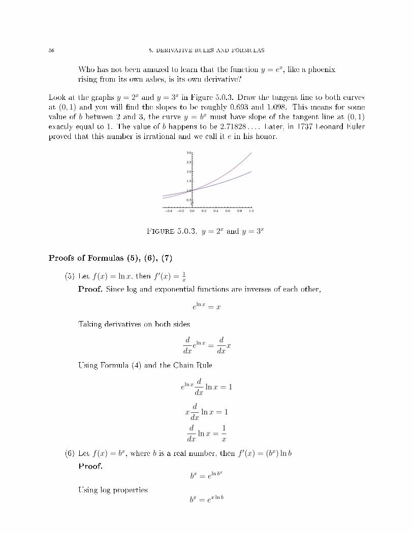
56 5. DERIVATIVE RULES AND FORMULAS
Who has not been amazed to learn that the function y = ex, like a phoenixrising from its own ashes, is its own derivative?
Look at the graphs y = 2x and y = 3x in Figure 5.0.3. Draw the tangent line to both curvesat (0, 1) and you will �nd the slopes to be roughly 0.693 and 1.098. This means for somevalue of b between 2 and 3, the curve y = bx must have slope of the tangent line at (0, 1)exactly equal to 1. The value of b happens to be 2.71828 . . . . Later, in 1737 Leonard Eulerproved that this number is irrational and we call it e in his honor.
Figure 5.0.3. y = 2x and y = 3x
Proofs of Formulas (5), (6), (7)
(5) Let f(x) = ln x, then f ′(x) = 1x
Proof. Since log and exponential functions are inverses of each other,
elnx = x
Taking derivatives on both sides
d
dxelnx =
d
dxx
Using Formula (4) and the Chain Rule
elnxd
dxlnx = 1
xd
dxlnx = 1
d
dxlnx =
1
x
(6) Let f(x) = bx, where b is a real number, then f ′(x) = (bx) ln b
Proof.bx = eln b
x
Using log propertiesbx = ex ln b

5. DERIVATIVE RULES AND FORMULAS 57
Taking derivatives on both sides and using Formula (4) and the Chain Rule
d
dxbx =
d
dxex ln b
= ex ln bd
dxx ln b
= ex ln b(lnb)
= eln bx
(lnb)
= bx(lnb)
(7) Let f(x) = logb x where b is a real number, then f ′(x) = 1x ln b
Proof.blogb x = x
Taking derivatives on both sides
d
dxblogb x =
d
dxx
Using Formula (6) and the Chain Rule
blogb x ln b(d
dxlogb x) = 1
x ln b(d
dxlogb x) = 1
d
dxlogb x =
1
x ln b�
Next, we give a short alternate proof of Formula (7) using the Change of Baseformula for logs. If we know logb x then we can �nd loga x for any desired base a asfollows:
loga x =logb x
logb a.
Alternate Proof of Formula (7). We have to �nd the derivative of f(x) = logb x.Using the Change of Base formula, we can change the base to e as follows:
f(x) = logb x =lnx
ln b= (
1
ln b) lnx
Using Formula (5) and the fact that ln b is a constant
f ′(x) =1
x ln b.
�
That's it! As promised it is a short proof.

58 5. DERIVATIVE RULES AND FORMULAS
Example 5.4. Find the derivatives of the following functions:
(1) y = xex
(2) y = x2ex
(3) y = x2bx
(4) y = (x2 + 2x+ 1) lnx
(5) y = logb xx2+1
Solutions.
(1) y = xex
dy
dx= x
d
dxex + ex
d
dxx
= xex + ex = ex(x+ 1)
(2) y = x2ex
dy
dx= x2
d
dxex + ex
d
dxx2
= x2ex + ex(2x) = xex(x+ 2)
(3) y = x2bx
dy
dx= x2
d
dxbx + bx
d
dxx2
= x2bx ln b+ bx(2x) = xbx(x ln b+ 2)
(4) y = (x2 + 2x+ 1) lnx
dy
dx= (x2 + 2x+ 1)
d
dxlnx+ (lnx)
d
dx(x2 + 2x+ 1)
= (x2 + 2x+ 1)1
x+ (lnx)(2x+ 2)

5. DERIVATIVE RULES AND FORMULAS 59
(5) y = logb xx2+1
=d
dx
(x2 + 1) ddx
logb x− (logb x) ddx
(x2 + 1)
(x2 + 1)2
=(x2 + 1) 1
x ln b− (logb x)(2x)
(x2 + 1)2
�
The second derivative of a function is the derivative of the derivative. The third derivativeis the derivative taken three times, and so on. The nth derivative is denoted as d2y
dx2. These
derivatives are called higher order derivatives.
Example 5.5. Find the second derivative of the following functions:
(1) y = x3 + 5x2 − 2x− 1
(2) y = xex
Solutions.
(1) y = x3 + 5x2 − 2x− 1dy
dx= 3x2 + 10x− 2
d2y
dx2= 6x+ 10
(2) y = xex
dy
dx= xex + ex = ex(x+ 1)
d2x
dy2= ex
d
dx(x+ 1) + (x+ 1)
d
dxex
= ex + (x+ 1)ex
= ex(x+ 2)
Former President of the American Mathematical Society Hugo Rossi noted in a columnin the AMS Notices Vol. 43 No. 10:
In the fall of 1972 President Nixon announced that the rate of increase ofin�ation was decreasing. This was the �rst time a sitting president usedthe third derivative to advance his case for reelection...Was President Nixon
60 5. DERIVATIVE RULES AND FORMULAS
telling us that the economy was getting better? Did his listeners understandthat in fact the in�ation rate was still increasing and thus the economy stillworsening?
In�ation is de�ned as a sustained increase in the general price level of goods and servicesin an economy over a period of time. So if x represents goods and services and y their prices,in�ation is the rate of change in price. In other words in�ation is the �rst derivative. Therate of change of in�ation is the second derivative, and the rate of change of the rate ofchange of in�ation is the third derivative.
Practice Problems
(1) Di�erentiate using the sum, di�erence, product and quotient rules.
a) y = x4 + 3x2 − 2
b) y = (1 + 4x)(x2 + x)
c) y = x2+1x2−1
d) y = x2+4x+3√x
e) y = x3
1−x2
f) y = x2+2x4−3x2+1
(2) Di�erentiate. In addition to the above rules, the Chain Rule is needed for theseproblems.
a) y = (x4 + 3x2 − 2)2
b) y = (4x− x2)100
c) y = 4√x3 + 2x+ 1
d) y = (x4 + 1)23
e) y = 1(x4+1)3
f) y = (1 + 4x)5(3 + x− x2)8
g) y =(x2+1x2−1
)3h) y =
√x−1x+1
(3) Di�erentiate.
a) y = e2x
b) y = e1−x
5. DERIVATIVE RULES AND FORMULAS 61
c) y = ex2−2x
d) y = e−x2
e) y = e−3x2
f) y = xex
g) y = ex
x+1
h) y = (ex + e−x)3
i) y = ex−e−x2
j) y = x2ex
k) y = x2ex − 2xex + 2ex
l) y = 32x
m) y = 21−x
n) y = 5x2−2x
o) y = 2−x2
p) y = 2−3
x2
q) y = x3x
r) y = 2x
x+1
(4) Di�erentiate.
a) y = ln 2x
b) y = log10 2x
c) y = log10 x3
d) y = ln(x2 + 5x)
e) y = log3(x2 + 5x)
f) y = lnxln 2x+1
g) y = lnxx2
h) y = 1+lnx1−lnx
i) y = 1lnx
(5) Find the equation of the tangent line to the curve at the indicated point.
a) y = x2 at (3, 9)
b) y = 1xat (1, 1)
c) y = x52 at (3, 3
52 )

62 5. DERIVATIVE RULES AND FORMULAS
(6) The equation of motion of a particle is given by y = 40t− 16t2 where y is in metersand t is in seconds. Velocity is the rate of change of distance (it is speed with adirection). Acceleration is the rate of change of velocity.
a) Find the velocity as a function of t.
b) Find the velocity when t = 2.
c) Find the acceleration as a function of t.
d) Find the acceleration when t = 2.
(7) Suppose a rock is thrown straight up in the air with an initial velocity of 40 feet persecond. Its height after t seconds is given by y = 40t− 16t2.
a) Find the velocity when t = 2.
b) At what time will the rock hit the surface?
c) With what velocity will the rock hit the surface?
CHAPTER 6
More Derivative Formulas
This chapter is essentially a continuation of the previous chapter with more formulas. Wewill study the derivatives of the six trigonometric functions and the six inverse trigonometricfunctions adding twelve more formulas to the previous list of six formulas and four rules. 1
British author William Somerset Maugham said
There are three rules for writing a novel.Unfortunately, no one knows what they are.
Fortunately, we have many wonderful rules for �nding derivatives that make things quiteeasy. We don't always get so lucky, not in math, not in anything else. So when there arerules that work why not study them for their own sake and �nd pleasure in the symmetryand beauty of the rules? From now on we will use the dy
dxnotation most of the time.
Theorem 6.1. (Derivatives of the six trigonometric functions)
(1) ddx
sinx = cosx
(2) ddx
cosx = − sinx
(3) ddx
tanx = sec2 x
(4) ddx
cotx = − csc2 x
(5) ddx
secx = secx tanx
(6) ddx
cscx = − cscx cotx
We will give an informal proof for (1) since it involves two limits that cannot be found bythe techniques in Chapter 3 and formal proofs for the rest. The formal proof of (1) appearsin Chapter 12. The proofs of Formulas (2) to (6) use the following trignometic identities:
• sin (π2− x) = cos x
• tanx = sinxcosx
• cotx = 1tanx
= cosxsinx
• secx = 1cosx
1 A student taking a course in Survey of Calculus or Business Calculus should focus on the twelveformulas and the two examples based on them, omitting all proofs.
63

64 6. MORE DERIVATIVE FORMULAS
• cscx = 1sinx
.
• sin2 x+ cos2 x = 1
• sec2 x− tan2 x = 1
• csc2 x− cot2 x = 1
But before looking at the proofs let us use these formulas in examples.
Example 6.2. Find the derivatives of the following functions:
(1) y = x2 sinx
(2) y = ecosx
(3) y = esec 3x
(4) y = secx1+tanx
Solutions.
(1) y = x2 sinx
dy
dx= x2
dy
dxsinx+ sinx
d
dxx2
= (x2)(cosx) + (sin x)(2x)
(2) y = ecosx
dy
dx= esec 3x
d
dxsec 3x
= esec 3x(sec 3x tan 3x)d
dx3x
= esec 3x(sec 3x tan 3x)(3)
(3) y = esec 3x
dy
dx= ecosx
d
dxcosx
= ecosx(− sinx)

6. MORE DERIVATIVE FORMULAS 65
(4) y = secx1+tanx
dy
dx=
(1 + tan x) ddx
secx− (secx) ddx
(1 + tanx)
(1 + tan x)2
=(1 + tan x) secx tanx− (secx) sec2 x
(1 + tanx)2
=(1 + tan x) secx tanx− sec3 x
(1 + tan x)2
�
Note that it may be possible to simply further using identities and get an elegant �nalanswer, but for the most part, this much simpli�cation is enough. However, if we have to�nd the second derivative, then more simplication is needed to get an expression easier todi�erentiate again.
Informal Proof of (1). Using the de�nition of the derivative
d
dxsinx =
sin(x+ h)− sinx
h
= limh→0
sinx cosh+ cosx sinh− sinx
h
= limh→0
sinx cosh− sinx+ cosx sinh
h
= limh→0
sinx(cosh− 1) + cos x sinh
h
= limh→0
sinx limh→0
cosh− 1
h+ lim
h→0cosx lim
h→0
sinh
h
We saw the graph of y = sinxx
in Figure 1.0.14. Recall that limx→0
sinxx
= 1. Similarly, the graph
of y = cosx−1x
is shown in Figure 6.0.1. Observe that limx→0
cosx−1x
= 0. So
d
dxsinx = lim
h→0sinx lim
h→0
cosh− 1
h+ lim
h→0cosx lim
h→0
sinh
h= (sinx)(0) + (cos x)(1)
= cosx.
�
Formal Proofs of (2) to (6).
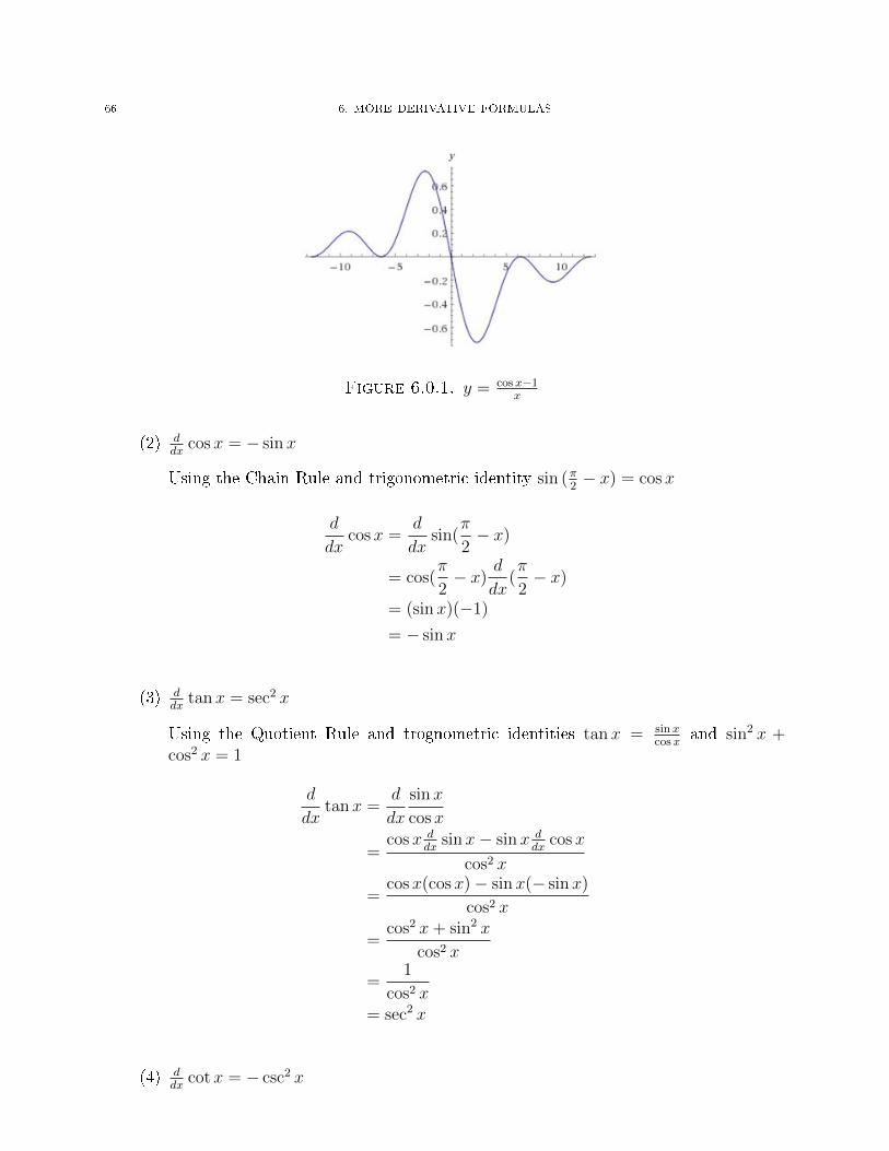
66 6. MORE DERIVATIVE FORMULAS
Figure 6.0.1. y = cosx−1x
(2) ddx
cosx = − sinx
Using the Chain Rule and trigonometric identity sin (π2− x) = cos x
d
dxcosx =
d
dxsin(
π
2− x)
= cos(π
2− x)
d
dx(π
2− x)
= (sinx)(−1)
= − sinx
(3) ddx
tanx = sec2 x
Using the Quotient Rule and trognometric identities tanx = sinxcosx
and sin2 x +cos2 x = 1
d
dxtanx =
d
dx
sinx
cosx
=cosx d
dxsinx− sinx d
dxcosx
cos2 x
=cosx(cosx)− sinx(− sinx)
cos2 x
=cos2 x+ sin2 x
cos2 x
=1
cos2 x= sec2 x
(4) ddx
cotx = − csc2 x

6. MORE DERIVATIVE FORMULAS 67
Using the Quotient Rule and trogonometric identities cotx = cosxsinx
and sin2 x +cos2 x = 1
d
dxcotx =
d
dx
cosx
sinx
=sinx d
dxcosx− cosx d
dxsinx
sin2 x
=sinx(− sinx)− cosx(− cosx)
cos2 x
=−(sin2 x+ cos2 x)
cos2 x
=1
sin2 x= csc2 x
(5) ddx
secx = secx tanx
Using the Power Rule and trigonometric identity secx = 1cosx
d
dxsecx =
d
dx
1
cosx
=d
dx(cosx)−1
= −(cosx)−2d
dxcosx
= − 1
cos2 x(− sinx)
=1
cosx
sinx
cosx= secx tanx
(6) ddx
cscx = − cscx cotx
Using the Power Rule and trigonometric identity cscx = 1sinx
d
dxcscx =
d
dx
1
sinx
=d
dx(sinx)−1
= −(sinx)−2d
dxsinx
= − 1
sin2 xcosx
= − 1
sinx
cosx
sinx= − cscx cotx
68 6. MORE DERIVATIVE FORMULAS
�
Theorem 6.3. (Derivatives of the six inverse trigonometric functions)
(1) ddx
sin−1 x = 1√1−x2
(2) ddx
cos−1 x = − 1√1−x2
(3) ddx
tan−1 x = 11+x2
(4) ddx
cot−1 x = − 1(1+x2)
(5) ddx
sec−1 x = 1|x|√x2−1
(6) ddx
csc−1 x = − 1|x|√x2−1
Example 6.4. Find the derivative:
(1) y = x tan−1 x
(2) y = x tan−1√x
(3) y = 1sin−1 x
Solutions.
(1) y = x tan−1 x
dy
dx= x
d
dxtan−1 x+ tan−1 x
d
dxx
= x1
1 + x2+ (tan−1 x)(1) =
x
1 + x2+ tan−1 x
(2) y = x tan−1√x
dy
dx= x
d
dxtan−1
√x+ tan−1
√xd
dxx
= x1
1 + x2d
dx
√x+ tan−1
√x
=x
1 + x21√x
+ tan−1√x
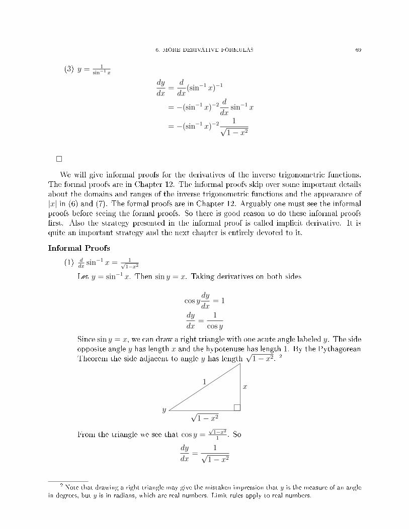
6. MORE DERIVATIVE FORMULAS 69
(3) y = 1sin−1 x
dy
dx=
d
dx(sin−1 x)−1
= −(sin−1 x)−2d
dxsin−1 x
= −(sin−1 x)−21√
1− x2
�
We will give informal proofs for the derivatives of the inverse trigonometric functions.The formal proofs are in Chapter 12. The informal proofs skip over some important detailsabout the domains and ranges of the inverse trigonometric functions and the appearance of|x| in (6) and (7). The formal proofs are in Chapter 12. Arguably one must see the informalproofs before seeing the formal proofs. So there is good reason to do these informal proofs�rst. Also the strategy presented in the informal proof is called implicit derivative. It isquite an important strategy and the next chapter is entirely devoted to it.
Informal Proofs
(1) ddx
sin−1 x = 1√1−x2
Let y = sin−1 x. Then sin y = x. Taking derivatives on both sides
cos ydy
dx= 1
dy
dx=
1
cos y
Since sin y = x, we can draw a right triangle with one acute angle labeled y. The sideopposite angle y has length x and the hypotenuse has length 1. By the PythagoreanTheorem the side adjacent to angle y has length
√1− x2. 2
y
1x
√1− x2
From the triangle we see that cos y =√1−x21
. So
dy
dx=
1√1− x2
2 Note that drawing a right triangle may give the mistaken impression that y is the measure of an anglein degrees, but y is in radians, which are real numbers. Limit rules apply to real numbers.

70 6. MORE DERIVATIVE FORMULAS
(2) ddx
cos−1 x = − 1√1−x2
Let y = cos−1 x. Then cos y = x. Taking derivatives on both sides
− sin ydy
dx= 1
dy
dx= − 1
sin y
Since cos y = x, we can draw a right triangle with one acute angle labeled y. Theside adjacent to angle y has length x and the hypotenuse has length 1. By thePythagorean Theorem the side opposite angle y has length
√1− x2.
y
1 √1− x2
x
From the triangle we see that cos y =√1−x21
. So
dy
dx= − 1√
1− x2
(3) ddx
tan−1 x = 11+x2
Let y = tan−1 x. Then tan y = x. Taking derivatives on both sides
sec2 ydy
dx= 1
dy
dx=
1
sec2 y
Since tan y = x, we can draw a right triangle with one acute angle labeled y. Theside opposite angle y has length x and the side adjacent to angle y has length 1. Bythe Pythagorean Theorem the hypotenuse has length 1 + x2.
y
1 + x2x
1
From the triangle we see that sec y = 1+x2
1. So
dy
dx=
1
sec2 y=
1
1 + x2

6. MORE DERIVATIVE FORMULAS 71
(4) ddx
cot−1 x = − 1(1+x2)
Let y = cot−1 x. Then cot y = x. Taking derivatives on both sides
− csc2 ydy
dx= 1
dy
dx= − 1
csc2 y
Since cot y = x, we can draw a right triangle with one acute angle labeled y. Theside adjacent to angle y has length x and the side opposite angle y has length 1. Bythe Pythagorean Theorem the hypotenuse has length 1 + x2.
y
1 + x21
x
From the triangle we see that csc y = 1+x2
1. So
dy
dx= − 1
csc2 y= − 1
1 + x2
(5) ddx
sec−1 x = 1|x|√x2−1
Let y = sec−1 x. Then sec y = |x|. 3 Taking derivatives on both sides
sec y tan ydy
dx= 1
dy
dx=
1
sec y tan y
Since sec y = |x|, we can draw a right triangle with one acute angle labeled y. Theside adjacent to angle y has length 1 and the hypotenuse has length |x|. By thePythagorean Theorem the side opposite angle y has length
√x2 − 1.
y
|x| √x2 − 1
1
From the triangle we see that sec y = |x|1and tan y =
√x2−11
. So
dy
dx=
1
sec y tan y=
1
|x|√x2 − 1
3To see why we have |x| here were must take a took at the formal proof in Appendix D. Without theformal proof this must be simply believed.

72 6. MORE DERIVATIVE FORMULAS
(6) ddx
csc−1 x = − 1|x|√x2−1
Let y = csc−1 x. Then csc y = |x|.Taking derivatives on both sides
− csc y cot ydy
dx= 1
dy
dx= − 1
csc y cot y
Since csc y = |x|, we can draw a right triangle with one acute angle labeled y. Theside opposite to angle y has length 1 and the hypotenuse has length |x|. By thePythagorean Theorem the side adjacent to angle y has length
√x2 − 1.
y
|x|1
√x2 − 1
From the triangle we see that csc y = |x|1and cot y =
√x2−11
. So
dy
dx= − 1
csc y cot y= − 1
|x|√x2 − 1
�
Practice Problems
(1) Find the derivative:
a) y = cosx
b) y = tanx
c) y = cscx
d) y = secx
e) y = cotx
f) y = sin−1 x
g) y = cos−1 x
h) y = tan−1 x
(2) Find the derivative:
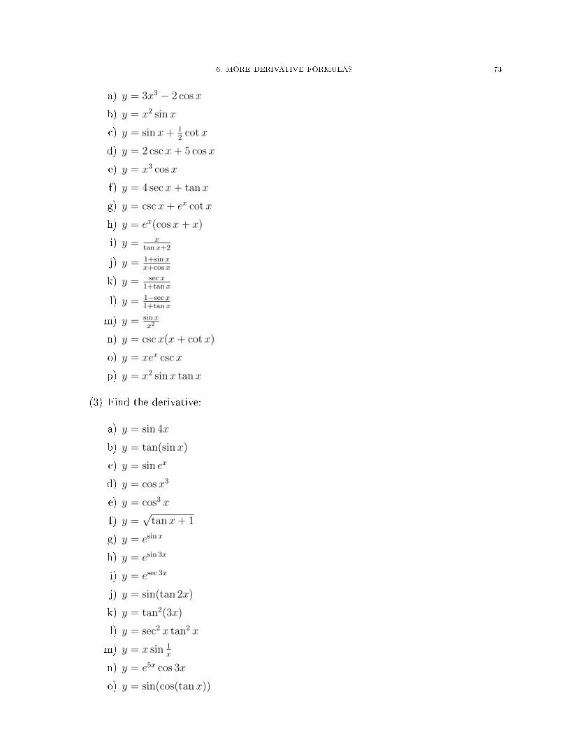
6. MORE DERIVATIVE FORMULAS 73
a) y = 3x3 − 2 cosx
b) y = x2 sinx
c) y = sinx+ 12
cotx
d) y = 2 csc x+ 5 cosx
e) y = x3 cosx
f) y = 4 sec x+ tanx
g) y = cscx+ ex cotx
h) y = ex(cosx+ x)
i) y = xtanx+2
j) y = 1+sinxx+cosx
k) y = secx1+tanx
l) y = 1−secx1+tanx
m) y = sinxx2
n) y = cscx(x+ cotx)
o) y = xex cscx
p) y = x2 sinx tanx
(3) Find the derivative:
a) y = sin 4x
b) y = tan(sinx)
c) y = sin ex
d) y = cosx3
e) y = cos3 x
f) y =√
tanx+ 1
g) y = esinx
h) y = esin 3x
i) y = esec 3x
j) y = sin(tan 2x)
k) y = tan2(3x)
l) y = sec2 x tan2 x
m) y = x sin 1x
n) y = e5x cos 3x
o) y = sin(cos(tanx))
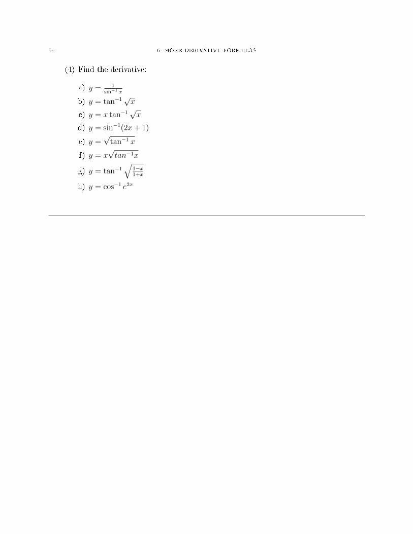
74 6. MORE DERIVATIVE FORMULAS
(4) Find the derivative:
a) y = 1sin−1 x
b) y = tan−1√x
c) y = x tan−1√x
d) y = sin−1(2x+ 1)
e) y =√
tan−1 x
f) y = x√tan−1x
g) y = tan−1√
1−x1+x
h) y = cos−1 e2x
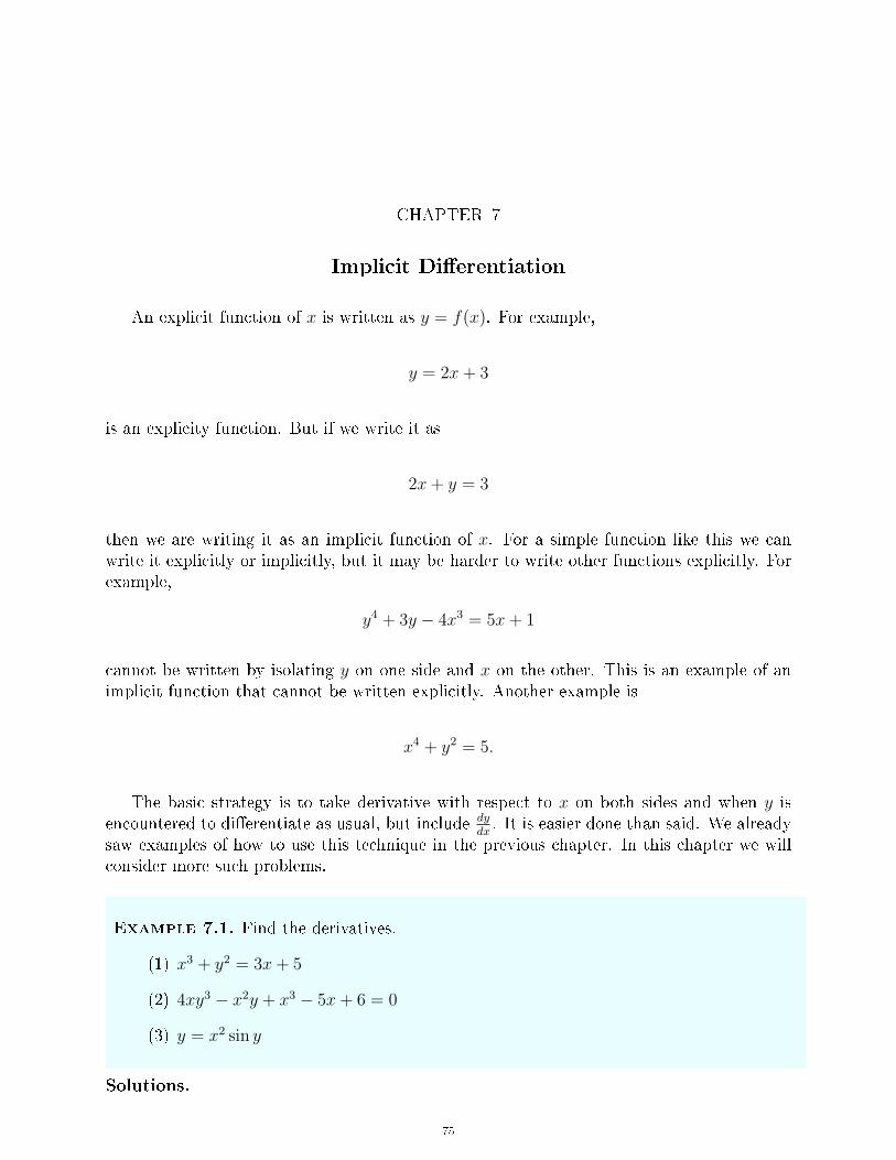
CHAPTER 7
Implicit Di�erentiation
An explicit function of x is written as y = f(x). For example,
y = 2x+ 3
is an explicity function. But if we write it as
2x+ y = 3
then we are writing it as an implicit function of x. For a simple function like this we canwrite it explicitly or implicitly, but it may be harder to write other functions explicitly. Forexample,
y4 + 3y − 4x3 = 5x+ 1
cannot be written by isolating y on one side and x on the other. This is an example of animplicit function that cannot be written explicitly. Another example is
x4 + y2 = 5.
The basic strategy is to take derivative with respect to x on both sides and when y isencountered to di�erentiate as usual, but include dy
dx. It is easier done than said. We already
saw examples of how to use this technique in the previous chapter. In this chapter we willconsider more such problems.
Example 7.1. Find the derivatives.
(1) x3 + y2 = 3x+ 5
(2) 4xy3 − x2y + x3 − 5x+ 6 = 0
(3) y = x2 sin y
Solutions.
75
76 7. IMPLICIT DIFFERENTIATION
(1) x3 + y2 = 3x+ 5
d
dx(x3 + y2) =
d
dx(3x+ 5)
d
dxx3 +
d
dxy2 =
d
dx3x+
d
dx5
3x2 + 2ydy
dx= 3 + 0
2ydy
dx= −3x2 + 3
dy
dx=−3x2 + 3
2y
(2) 4xy3 − x2y + x3 − 5x+ 6 = 0
d
dx(4xy3 − x2y + x3 − 5x+ 6) =
d
dx0
d
dx4xy3 − d
dxx2y +
d
dxx3 − d
dx5x+
d
dx6 =
d
dx0
4xd
dxy3 + y3
d
dx(4x)− [x2
dy
dx− y d
dxx2] + 3x2 + 5 = 0
4x(3y3)dy
dx+ y3(4)− [x2
dy
dx− y(2x)] + 3x2 + 5 = 0
12xy3dy
dx+ 4y3 − x2 dy
dx+ 2xy + 3x2 + 5 = 0
dy
dx[12xy3 − x2] = −4y3 − 2xy − 3x2 − 5
dy
dx=−4y3 − 2xy − 3x2 − 5
12xy3 − x2
(3) y = x2 sin y
dy
dx= x2
d
dxsin y + sin y
d
dxx2
dy
dx= x2 cos y
dy
dx+ (sin y)(2x)
dy
dx(1− x2 cos y) = 2x sin y
dy
dx=
2x sin y
1− x2 cos y
�

7. IMPLICIT DIFFERENTIATION 77
We can use implicit di�erentiation to �nd the derivatives of f(x) = lnx and f(x) = bx.Many would consider these proofs easier than the previous ones in Chapter 5. So it is worthreviwing the next example even though we saw it earlier.
Example 7.2. Find the derivatives.
(1) y = lnx
(2) y = bx
Solutions.
(1) y = lnx
Since y = lnx by de�nitioney = x
Taking derivatives on both sides and using implicit di�erentiation
dy
dxey =
d
dxx
eydy
dx= 1
dy
dx=
1
ey
dy
dx=
1
x
(2) Since y = bx we can take log on both sides to get
ln y = ln bx
Using log propertiesln y = x ln b
Taking derivatives on both sides and using implicit di�erentiation
d
dxln y =
d
dxx ln b
1
y
dy
dx= ln b
dy
dx= y ln b
dy
dx= bx ln b

78 7. IMPLICIT DIFFERENTIATION
�
The technique of taking log on both sides requires some explanation. Suppose f is a one-to-one function, then we can compose f with another one-to-one function g to get g ◦ f . Thisis what we are doing when we take log on both sides. The log function is one-to-one. 1 Thismeans
m = n ⇐⇒ logbm = logbn
The next set of problems involve a new function
f(x) = xx
whose graph is shown in Figure 7.0.1. This is not a power function nor an exponentialfunction. If x = 1, then y = 11 = 1. Between 0 and 1 the function dips and past 1 it rises.The function is not de�ned at 0. When x < 0 the situation is more complicated. For example,if x = −2, y = (−2)( − 2) = 1
(−2)2 = 14. If x = −3, then y = (−3)( − 3) = 1
(−3)3 = 1−27 .
However, if x = 12, then y = (−0.5)( − 0.5) = 1
(−0.5)−0.5 , which is a complex number. It ishard to write the domain since the real and complex values of the function are intermingled.Figure 7.0.1 shows both the real and complex portions of the graph.
Figure 7.0.1. y = xx
Example 7.3. Find the derivatives.
(1) y = xx
(2) y = x√x
(3) y = xcosx
1 A function doesn't have to be one-to-one, but then things get a bit messy and must be analyzed ona case-by-case basis. For example, when solving radical equations, we square both sides and the squaringfunction is not one-to-one. As a result we get extraneaous solutions.
7. IMPLICIT DIFFERENTIATION 79
The strategy here is to take log on both sides and to use the log property
logb xt = t logb x.
Solution.
(1) y = xx
Starting with y = xx, take ln on both sides to get
ln y = lnxx
ln y = x lnx
1
y
dy
dx= x
d
dxlnx+ (lnx)
d
dxx
1
y
dy
dx= x
1
x+ (lnx)(1)
dy
dx= y[1 + ln x]
dy
dx= xx[1 + ln x]
(2) y = x√x
ln y = lnx√x
ln y =√x lnx
1
y
dy
dx=√xd
dxlnx+ (lnx)
d
dx
√x
1
y
dy
dx=√x
1
x+ (lnx)
1
2√x
1
y
dy
dx=
1√x
+ (lnx)1
2√x
1
y
dy
dx=
1√x
[1 +lnx
2]
dy
dx=
y√x
[1 +lnx
2]
dy
dx=x√x
√x
[1 +lnx
2]
80 7. IMPLICIT DIFFERENTIATION
(3) y = xcosx
lny = xcosx
ln y = lnxcosx
ln y = cosx lnx
1
y
dy
dx= cosx
d
dxlnx+ (lnx)
d
dxcosx
1
y
dy
dx= (cosx)(
1
x) + (ln x)(− sinx)
dy
dx= y[
cosx
x+ (lnx)(− sinx)]
dy
dx= xcosx[
cosx
x+ (lnx)(− sinx)]
�
Example 7.4. Find the second derivatives.
(1) x2 + y2 = 10
(2) x4 + y4 = 10
Previously we did not simplify the derivative once we found them since the emphasis wason knowing and using the formulas and rules correctly. Now it makes sense to simplify the�rst derivative as much as possible before �nding the second derivative. So the solutions ofthese problems can get quite long.
Solution.
(1)x2 + y2 = 10
d
dxx2 +
d
dxy2 =
d
dx10
2x+ 2ydy
dx= 0
x+ ydy
dx= 0
dy
dx= −x
y

7. IMPLICIT DIFFERENTIATION 81
d2y
dx2= −
y ddxx− x d
dxy
y2
= −y − x dy
dx
y2Put
dy
dx= −x
y
= −y − x−x
y
y2
= −y2 + x2
y3Put x2 + y2 = 10
= −10
y3
(2)x4 + y4 = 10
d
dxx4 +
d
dxy4 =
d
dx10
4x3 + 4y3dy
dx= 0
x3 + y3dy
dx= 0
dy
dx= −x
3
y3

82 7. IMPLICIT DIFFERENTIATION
d2y
dx2= −
y3 ddxx3 − x3 d
dxy3
y6
= −y33x2 − x33y2 dy
dx
y6Put
dy
dx= −x
3
y3
= −3x2y3 − 3x3y2−x
3
y3
y6
= −3x2y3 + 3x6
y
y6
= −3x2y4 + 3x6
y7
= −3x2(y4 + x4)
y7Put x4 + y4 = 10
= −3x2(10)
y7
= −30x2
y3
�
This chapter concludes the topic of derivatives and how to �nd them. In the next chapterwe will learn a method for �nding limits based on the derivative. In subsequent chapters wewill see some fascinating real world problems.
Practice Problems
(1) Find the derivatives.
a) x2 + y2 = 36
b) x12 + y
12 = 9
c) x3 − xy + y2 = 4
d) x3y3 − y = x
e) x3 − 3x2y + 2xy2 = 12
f) sinx+ 2 cos 2y = 1
g) sinx = x(1 + tan y)
h) y = sin(xy)

7. IMPLICIT DIFFERENTIATION 83
(2) Find the second derivative.
a) y = 4x32
b) y = xx−1
c) y = 3 sin x
d) y = secx
e) 9x2 + y2 − 9
f) x3 + y3 = 1
g) x4 + y4 = 16
h)√x+√y = 1
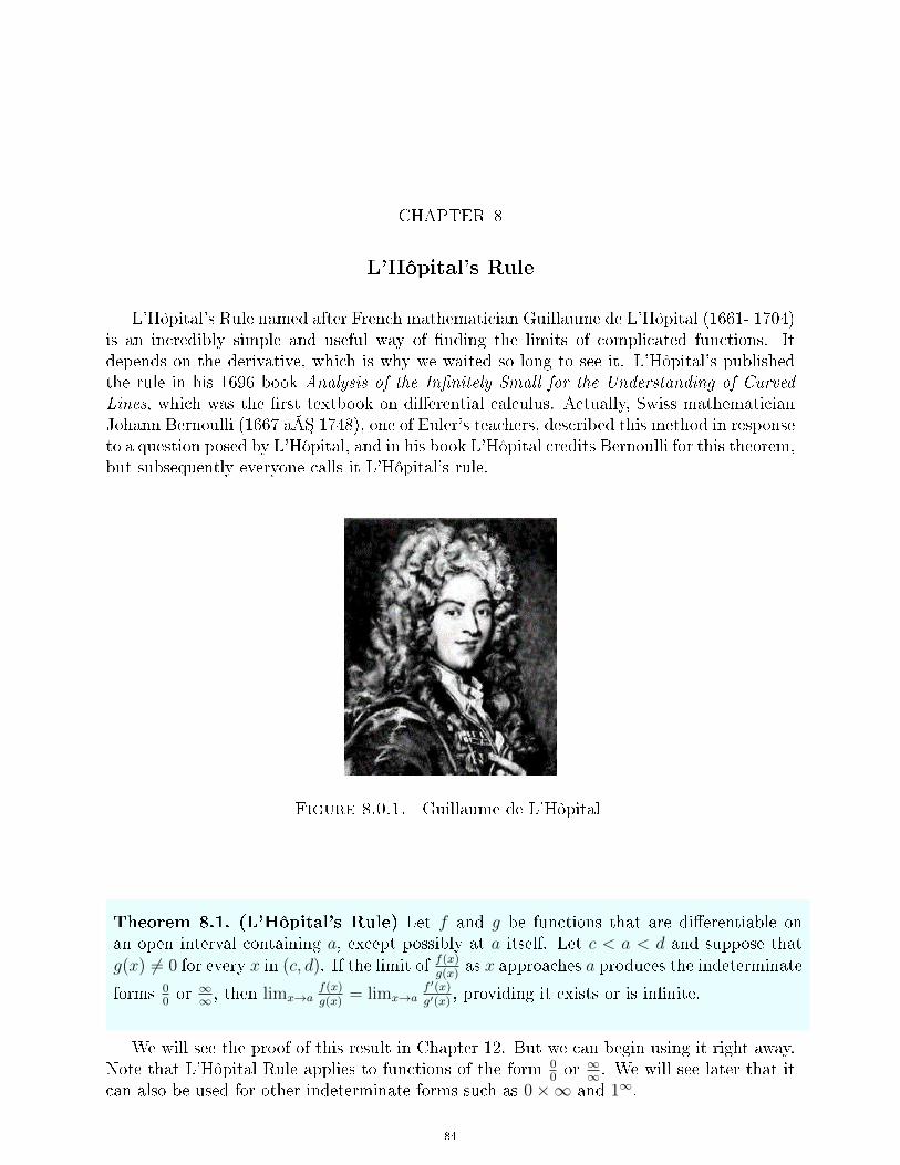
CHAPTER 8
L'Hôpital's Rule
L'Hôpital's Rule named after French mathematician Guillaume de L'Hôpital (1661- 1704)is an incredibly simple and useful way of �nding the limits of complicated functions. Itdepends on the derivative, which is why we waited so long to see it. L'Hôpital's publishedthe rule in his 1696 book Analysis of the In�nitely Small for the Understanding of Curved
Lines, which was the �rst textbook on di�erential calculus. Actually, Swiss mathematicianJohann Bernoulli (1667 â�� 1748), one of Euler's teachers, described this method in responseto a question posed by L'Hôpital, and in his book L'Hôpital credits Bernoulli for this theorem,but subsequently everyone calls it L'Hôpital's rule.
Figure 8.0.1. Guillaume de L'Hôpital
Theorem 8.1. (L'Hôpital's Rule) Let f and g be functions that are di�erentiable onan open interval containing a, except possibly at a itself. Let c < a < d and suppose thatg(x) 6= 0 for every x in (c, d). If the limit of f(x)
g(x)as x approaches a produces the indeterminate
forms 00or ∞∞ , then limx→a
f(x)g(x)
= limx→af ′(x)g′(x)
, providing it exists or is in�nite.
We will see the proof of this result in Chapter 12. But we can begin using it right away.Note that L'Hôpital Rule applies to functions of the form 0
0or ∞∞ . We will see later that it
can also be used for other indeterminate forms such as 0×∞ and 1∞.
84

8. L'HÔPITAL'S RULE 85
Example 8.2. Use L'Hôpital's Rule to �nd the limits, if possible.
(1) limx→1lnxx−1
(2) limx→∞ex
x2
(3) limx→∞lnx3√x
(4) limx→0tanx−xx3
Solution.
(1) Observe that limx→1lnxx−1 has 0
0form. So
limx→1
lnx
x− 1= lim
x→1
1x
1= 1
(2) Observe that limx→∞ex
x2has ∞∞ form. So
limx→∞
ex
x2= lim
x→∞
ex
2x
Now we can apply L'Hôpital Rule's again since limx→∞ex
2xagain has ∞∞ form. So
limx→∞
ex
2x= lim
x→∞
ex
2=∞
.
Putting it all together (without using so many words) we get
limx→∞
ex
x2= lim
x→∞
ex
2x
= limx→∞
ex
2x
= limx→∞
ex
2=∞

86 8. L'HÔPITAL'S RULE
(3) Observe that limx→∞lnx3√x has ∞∞ form. So
limx→∞
lnx3√x
= limx→∞
1x
13x−
23
= limx→∞
3
xx−23
= limx→∞
33√x
= 0
(4) Observe that limx→0tanx−xx3
has 00form.
limx→0
tanx− xx3
= limx→0
sec2 x− 1
3x2
= limx→0
2 sec2 x tanx
6x
=
(1
3limx→0
sec2 x
)·(
limx→0
tanx
x
)=
1
3· limx→0
sec2 x
1
=1
3· 1
=1
3
�
Next, let us consider problems of the type f(x)g(x) where one function tends to zero andthe other tends to ±∞. In such cases, it isn't clear whether f(x) or g(x) will dominate inthe limit. This kind of indeterminate form is of type 0 · ∞. Our strategy is to write f · g asf1g
or g1f
so that it will have either 00or ∞∞ form.
Example 8.3. Find the limits.
(1) limx→0+ x lnx
Solution.
8. L'HÔPITAL'S RULE 87
(1) We write limx→0+ x lnx as limx→0+lnx1x
which is in the −∞∞ form. So L'Hôpital's
Rule applies and we get
limx→0+
x lnx = limx→0+
lnx1x
= limx→0+
1x
− 1x2
= limx→0+
−x
= 0
�
Lastly, consider function of the indeterminate form 1∞. In this case, we take log on bothsides and turn it into a function of the form f(x)g(x) and use the previous approach.
Example 8.4. Find the limits.
(1) limx→∞(1 + 1
x
)x(2) limx→0+ (sinx)x
Solutions.
(1) Let y = limx→∞(1 + 1
x
)xand take ln on both sides
ln y = ln limx→∞
(1 +
1
x
)x= lim
x→∞x ln
(1 +
1
x
)= lim
x→∞
ln(1 + 1
x
)1x
= limx→∞
11+ 1
x
·(− 1x2
)− 1x2
(by L'Hôpital's Rule)
= limx→∞
1
1 + 1x
= 1
Since ln y = 1, it follows that y = e.
(2) Let y = limx→0+ (sinx)x and take ln on both sides.

88 8. L'HÔPITAL'S RULE
ln y = limx→0+
x ln(sinx)
= limx→0+
ln sinx1x
(which has∞∞
form)
= limx→0+
1sinx
cosx
− 1x2
= limx→0+
cotx
− 1x2
= limx→0+
−x2
tanx(which has
0
0form)
= − limx→0+
2x
sec2 x= 0
Since ln y = 0, it follows that y = e0 = 1.
�
Practice Problems
Find the limit if it exists.
(1) limx→1x2−1x2−x
(2) limx→1x9−1x5−1
(3) limx→2x2+x+6x−2
(4) limx→π2+
cosx1−sinx
(5) limx→0sin 4xtan 5x
(6) limx→0ex−1x3
(7) limx→0e3x−1x
(8) limx→∞x+x2
1−2x2
(9) limx→∞lnxx
(10) limx→0+lnxx
8. L'HÔPITAL'S RULE 89
(11) limx→∞ex
x3
(12) limx→0(1− x)1x
(13) limx→0+(tanx)x2
(14) limx→∞(lnx)1x
(15) limx→0+(1 + sin 4x)cotx
(16) limx→∞(ex + x)1x

CHAPTER 9
Related Rates
Related rates is the phrase used to describe the situation when two or more relatedvariables are changing with respect to time. The rate of change, as mentioned earlier, isanother expression for the derivative. For example, suppose water is draining from a conewith a hole in the bottom. We have the �xed height of the cone and the radius of its baseand the changing height of the water and radius of its base. At the begining they are thesame. After, for example, 10 seconds of water draining, the height of the water in the conechanges and will continue changing until all the water is drained out of the cone. The volumeof a cone is given by the formula
V =π
3r2h
shown in Figure 9.0.1 To �nd the volume of a cone and other geometric objects, type �Volumeof a cone� in Google Search and the interactive Google Calculator shown in Figure 9.0.1 willcome up.
Figure 9.0.1. V = π3r2h
There are three variables in this formula, V , r, and h, all changing at di�erent, butrelated, rates with respect to t. Suppose we di�erentiate both sides of the formula implicitlywith respect to t. Then by the product rule we get
dV
dt=π
3
[r2dh
dt+ h
d
dtr2]
dV
dt=π
3
[r2dh
dt+ 2rh
dr
dt
]The above equation is an equation with derivatives. It describes how the rate of change ofvolume V is related to the rates of change of height h and radius r. If we are given r, dr
dt, h
90
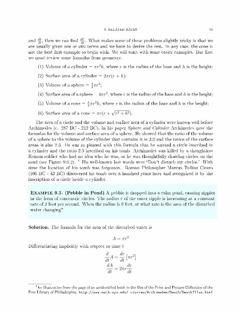
9. RELATED RATES 91
and dhdt, then we can �nd dV
dt. What makes some of these problems slightly tricky is that we
are usually given one or two terms and we have to derive the rest. In any case, the cone isnot the best �rst example to begin with. We will start with some easier examples. But �rstwe must review some formulas from geometry.
(1) Volume of a cylinder = πr2h, where r is the radius of the base and h is the height;
(2) Surface area of a cylinder = 2πr(r + h);
(3) Volume of a sphere = 43πr3;
(4) Surface area of a sphere = 4πr2, where r is the radius of the base and h is the height;
(5) Volume of a cone = π3πr2h, where r is the radius of the base and h is the height;
(6) Surface area of a cone = πr(r +√r2 + h2).
The area of a circle and the volume and surface area of a cylinder were known well beforeArchimedes (c. 287 BC - 212 BC). In his paper Sphere and Cylinder Archimedes gave theformulas for the volume and surface area of a sphere. He showed that the ratio of the volumeof a sphere to the volume of the cylinder that contains it is 2:3 and the ratios of the surfaceareas is also 2:3. He was so pleased with this formula that he wanted a circle inscribed ina cylinder and the ratio 2:3 inscribed on his tomb. Archimedes was killed by a thoughtlessRoman soldier who had no idea who he was, as he was thoughtfully drawing circles on thesand (see Figure 9.0.2). 1 His well-known last words were �Don't disturb my circles.� Withtime the location of his tomb was forgotton. Roman Philosopher Marcus Tullius Cicero(106 BC - 43 BC) discovered his tomb over a hundred years later and recognized it by theinscription of a circle inside a cylinder.
Example 9.1. (Pebble in Pond) A pebble is dropped into a calm pond, causing ripplesin the form of concentric circles. The radius r of the outer ripple is increasing at a constantrate of 2 foot per second. When the radius is 6 feet, at what rate is the area of the disturbedwater changing?
Solution. The formula for the area of the disturbed water is
A = πr2
Di�erentiating implicitly with respect to time t
d
dtA =
dr
dt
[πr2]
dA
dt= 2πr
dr
dt
1An illustration from the page of an unidenti�ed book in the �les of the Print and Picture Collection of theFree Library of Philadelphia. http://www.math.nyu.edu/ crorres/Archimedes/Death/DeathIllus.html
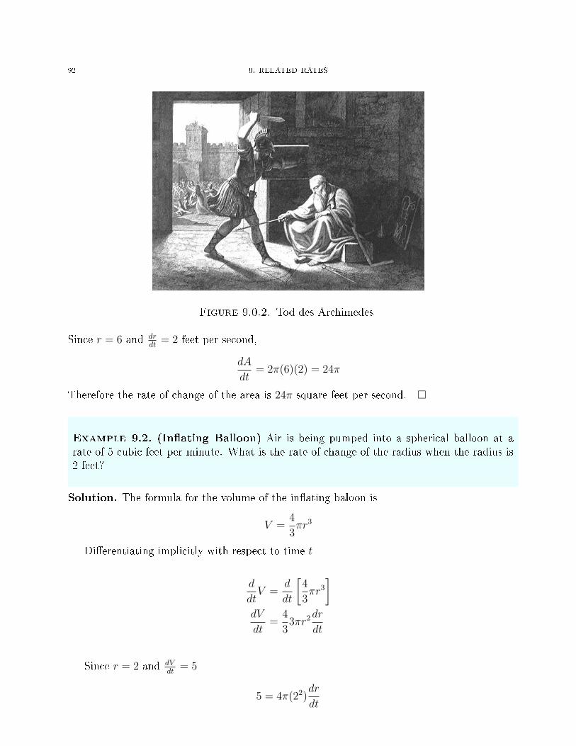
92 9. RELATED RATES
Figure 9.0.2. Tod des Archimedes
Since r = 6 and drdt
= 2 feet per second,
dA
dt= 2π(6)(2) = 24π
Therefore the rate of change of the area is 24π square feet per second. �
Example 9.2. (In�ating Balloon) Air is being pumped into a spherical balloon at arate of 5 cubic feet per minute. What is the rate of change of the radius when the radius is2 feet?
Solution. The formula for the volume of the in�ating baloon is
V =4
3πr3
Di�erentiating implicitly with respect to time t
d
dtV =
d
dt
[4
3πr3]
dV
dt=
4
33πr2
dr
dt
Since r = 2 and dVdt
= 5
5 = 4π(22)dr
dt

9. RELATED RATES 93
5 = 16πdr
dt
dr
dt=
5
16π
Therefore the rate of change of the radius is 516π
square feet per second. �
Example 9.3. (Flying Airplane) An airplane is �ying over a radar tracking station at aheight of 6 miles. Suppose the distance is decreasing at a rate of 400 miles per hour. Whatis the velocity of the plane when the distance is 10 miles?
radar
airplane
zy = 6
x
Solution. Since the triangle is a right triangle, by the Pythagorean Theorem
x2 + y2 = z2
where x is the horizontal distance, y is the vertical distance and the hypotenuse z is thedistance of the airplane from the station. In this problem, x and z are changing, but theheight of the plane is �xed at y = 6. So the equation is
x2 + 62 = z2
Di�erentiating implicitly with respect to time t
d
dtx2 +
d
dt62 =
d
dtz2
2xdx
dt= 2z
dz
dt
xdx
dt= z
dz
dt
We are given that y = 6 (which we already used) and z = 10. By the Pythagorean Theoremwe can �nd x as
x2 = z2 − y2 = 102 − 62 = 64
So x = 8. We are also given dzdt
= −400 (the negative sign stands for decreasing distance).
8dx
dt= 10(−400)
dx
dt= −500

94 9. RELATED RATES
The airplane is approaching the radar station at the rate of 500 miles per hour. �
Example 9.4. (Sliding Ladder) A ladder 10 feet long rests against a vertical wall. Ifthe base of the ladder slides away from the wall at a rate of 1 foot per second, how fast isthe top of the ladder sliding down the wall when the bottom is 6 feet away from the wall?
ladder base
ladder top
z = 10wall y
x
Solution. Since the triangle is a right triangle, by the Pythagorean Theorem
x2 + y2 = z2
where x is the horizontal distance of the ladder from the wall, y is the wall, and the hy-potenuse z is the length of the ladder. In this problem, x and y are changing, but the lengthof the ladder is �xed at z = 10. So the equation is
x2 + y2 = 102
Di�erentiating implicitly with respect to time t
d
dtx2 +
d
dty2 =
d
dt100
2xdx
dt+ 2y
dz
dt= 0
xdx
dt+ y
dz
dt= 0
We are given that z = 10 (which we already used) and x = 8. By the Pythagorean Theoremwe can �nd y as
y2 = z2 − x2 = 102 − 82 = 36
So y = 6. We are also given dxdt
= 1. We must �nd dxdt.
8(1) + 6dy
dt= 0
dy
dt= −8
6
The ladder is sliding down the wall at the rate of 1.3̄ feet per second. �
9. RELATED RATES 95
Example 9.5. (Moving Car) Car A is traveling west at 50 miles per hour and car B istraveling north at 60 miles per hour. Both are headed for the intersection of two roads. Atwhat rate are the cars approaching each other when car A is 0.3 miles from the intersectionand car B is 0.4 miles from the intersection?
Solution. Since the triangle is a right triangle, by the Pythagorean Theorem
x2 + y2 = z2
where x is the horizontal distance west travelled by Car A, y is the vertical distance northtravelled by the Car B, and the hypotenuse z is the distance between the cars, which isshrinking.
x2 + y2 = z2
Di�erentiating implicitly with respect to time t
d
dtx2 +
d
dty2 =
d
dtz2
2xdx
dt+ 2y
dz
dt= 2z
dz
dt
xdx
dt+ y
dz
dt= z
dz
dtWe are given that x = 0.3 and y = 0.4. By the Pythagorean Theorem we can �nd z as
z2 = x2 + y2 = 0.32 + 0.42 = 0.25
So z = 0.5. We are also given dxdt
= −50 miles per hour and dydt
= −60 miles per hour. Thesigns are negative because the cars are �approaching� the intersection. In other words thedistance between the cars and the intersection is decreasing.
xdx
dt+ y
dy
dt= z
dz
dt
0.3(−50) + 0.4(−60) = 0.5dz
dtdz
dt= −78
The cars are approaching each other at 78 miles per hour. �
Example 9.6. (Water Tank) A water tank has the shape of an inverted cone with a baseof radius of 2 meters and height 4 meters. If water is being pumped into the tank at a rateof 2 cubic meters per minute, �nd the rate at which the water level is rising when the wateris 3 meters deep.

96 9. RELATED RATES
Solution. The volume of a cone isV =
π
3r2h
where r is the radius of the base, h is the height of the cone. We are given r = 2 and h = 4.Based on this we can conclude r = h
2. (Note this is true only for this particular problem.)
V =π
3r2h
=π
3(h
2)2h
=πh3
12
Di�erentiate implicitly with respect to t
dV
dt=
3π
12h2dh
dt
2 =π
4h2dh
dtdh
dt=
8
9π
The rate at which the water level is rising is 89π
meters per minute. �
Example 9.7. A man walks along a straight path at a speed of 4 feet per second toward apole with a searchlight on top. The height of the searchlight is 20 feet and it is kept focusedon the man rotating downward as the man moves. At what rate is the searchlight rotatingwhen the man is 15 feet from the pole?
man
search light
zy = 20
x
Solution. From the above triangle
x2 + y2 = z2
where x is the distance of the man from the pole, y = 20 is the height of the searchlight(which is �xed) and the hypotenuse z is the distance of the man from the search light. Theequation to be used here is
tan θ =x
20

9. RELATED RATES 97
since we want the angle of rotation of the searchlight and it rotates downwards toward theman as he approaches the pole. Di�erentiating implicitly with respect to t gives
sec2 θdθ
dt=
1
20
dx
dt
In order to �nd dθdt
we need sec θ and dxdt. We are given that dx
dt= −4 feet per second. The
negative sign appears since the man is approaching the pole. But we have to �nd sec θ fromthe available information. Using the fact that x = 15 and y = 20, by the PythagoreanTheorem
z = x2 + y2 = 152 + 202 = 625
So z = 25 and from the right triangle we get
cos θ =20
25=
4
5
sosec θ =
5
4.
Putting it together we get
dx
dt= 20 sec2 θ
dθ
dt
−4 = 20
(5
4
)2dθ
dt
dθ
dt= − 4
20
(4
5
)2
= − 16
125
The searchlight is rotating at a rate of − 16125
radians per second. �
There are two things to note in the above problem. First the angle is negative since thesearchlight is rotating downward. Moreover, the number is angle measure in radians. Indegrees the angle is
− 16
125× 180
π≈ −7.34◦
Second we could have used x = 15 and y = 20 to write
tan θ =x
y=
15
20
and �nd θ = 36.87◦ using the inverse tangent key on a calculator. Then we could putθ = 36.87◦ in the related rates equation
sec2 θdθ
dt=
1
20
dx
dt

98 9. RELATED RATES
As you can see from the last two problems, if all the information is not directly given inthe statement of the problem itself, then the problem requires more thought. These sorts ofmulti-step problems, where you have to �gure out one thing and use it to get the next thing,and so on, are typical of real-world problems. However, the above problems are contrivedlike cardboard cut-outs of real-world problems. It is worth doing a few of these contrivedproblems to master the techniques and leave it at that.
Practice Problems
(1) A pebble is dropped in a calm pond causing ripples to form in concentric circles.The radius of the outer ripple is increasing at a constant rate of 1 foot per second.When the radius is 4 feet, at what rate is the area of disturbed water changing?
(2) Air is pumped into a spherical balloon at a rate of 5 cubic feet per minute. �nd therate of change of the radius when the radius is 3 feet.
(3) Air is pumped into a spherical balloon so that the volume increases at a rate of 100cubic centimeters per second. How fast is the radius of the balloon increasing whenthe diameter is 50 centimeters?
(4) If a snowball melts so that its surface area decreases at a rate of 2 square centimetersper minute, �nd the rate at which the diameter decrease when the diameter is 10centimeters.
(5) All edges of a cube are expanding at a rate of 3 centimeters per second. How fastis the volume changing when each edge is 10 centimeters?
(6) A water tank has the shape of an inverted circular cone with base radius 2 metersand height 4 meters. If water is being pumped into the tank at a rate of 2 cubicmeters per minute, �nd the rate at which the water level is rising when the wateris 3 meters deep.
(7) Gravel is being dumped from a conveyor belt at a rate of 30 cubic feet per minuteand forms a conical pile whose base diameter and height are equal. How fast is theheight of the pile increasing when the pile is 10 feet high?
(8) Sand is falling o� a conveyor belt onto a conical pile at a rate of 10 cubic feet perminute. The diameter of the base of the cone is three times the height. At whatrate is the height of the pile changing when the pile is 15 feet high?
(9) A conical tank with vertex down is 10 feet across at the top and 12 feet deep. Ifwater is �owing into the tank at a rate of 10 cubic feet per minute, �nd the rate ofchange of the depth of the water when the water is 8 feet deep.
(10) An airplane is �ying over a radar tracking station at a height of 6 miles. If thedistance between the plane and the station is decreasing at a rate of 400 miles perhour, when the distance is 10 miles, what is the speed of the plane?

9. RELATED RATES 99
(11) A ladder 10 feet long rests against a vertical wall. If the bottom of the ladder slidesaway from the wall at a rate of 1 foot per second, how fast is the top of the laddersliding down the wall, when the bottom is 6 feet from the wall?
(12) Car A is traveling west at 50 miles per hour and car B is traveling north at 60 milesper hour headed for the intersection of the two roads. At what rate are the carsapproaching each other when car A is 0.3 miles and car B is 0.4 miles from theintersection?
(13) Two cars start moving from the same point. One travels south at 60 miles per hourand the other travels west at 25 miles per hour. At what rate is the distance betweenthe cars increasing 2 hours later?

CHAPTER 10
Maxima and Minima
Arguably the whole purpose of derivatives is to determine the maximum and minimumof functions. Take a look at Figure 10.0.1. It shows the graph of the quadratic functionf(x) = −x2 + 8x + 20. Reading the graph from left to right, observe how the graph rises(increases) on the left reaches the highest point at the vertex and then falls (decreases) onthe right. Notice how the graph is rapidly increasing at �rst and then as it approaches thevertex, the rate of increase although still positive decreases. The rate of change is the slopeof the tangent line. Imagine small tangent lines draw at various points on the graph. At thevertex the tangent line becomes horizontal (the slope is zero). Then the slope of the tangentline gradually becomes negtive, slowly at �rst, then faster and faster.
Figure 10.0.1. f(x) = −x2 + 8x+ 20
We have an easy formula for �nding the vertex of a quadratic function f(x) = ax2 + bx+ c.The x-coordinate of the vertex is
x = − b
2a.
So the x-coordinate of vertex of f(x) = −x2 + 8x+ 20 is
x = − 8
2(−1)= 4.
The y-coordinate of the vertex is
f(4) = −(4)2 + 8(4) + 20 = −16 + 32 + 20 = 36.
Thus, the vertex of f(x) = −x2 + 8x + 20 is (4, 36). But what if the functions are f(x) =x4 − 8x2 + 16 or g(x) = x5 − 8x3 + 16x whose graphs are shown in Figure 10.0.2. We don't
100

10. MAXIMA AND MINIMA 101
Figure 10.0.2. f(x) = x4 − 8x2 + 16 (left) and g(x) = x5 − 8x3 + 16x (right)
have formulas for the highest and lowest points like we did for quadratic functions. You maythink that zooming into the graph will help, and it might work sometimes, but not always.In his article �Change we can believe in� Steven Strogatz describes local maxima and minimaas follows:
There's a more general principle at work here - things always change slowestat the top or the bottom. It's especially noticeable here in Ithaca. Duringthe darkest depths of winter, the days are not just unmercifully short;they barely improve from one to the next. Whereas now that spring ispopping, the days are lengthening rapidly. All of this makes sense. Changeis most sluggish at the extremes precisely because the derivative is zerothere. Things stand still, momentarily. This zero-derivative property ofpeaks and troughs underlies some of the most practical applications ofcalculus. It allows us to use derivatives to �gure out where a functionreaches its maximum or minimum, an issue that arises whenever we'relooking for the best or cheapest or fastest way to do something.
Let's take a careful look at a very familiar function, namely, f(x) = x2 whose graph isshown in Figure 10.0.3 alongside its derivative f ′(x) = 2x and second derivative f ′′(x) = 2.There is a close relationship between the graph of the function and the graph of its �rst andsecond derivative. Observe that
• Over the interval (−∞, 0), f is decreasing and f ′ is negative;
• Over the interval (0,∞), f is increasing and f ′ is negative;
• f is concave up and f ′′ is positive.
Similarly, the graph of f(x) = −x2 and its derivatives f ′(x) = −2x and f ′′(x) = 2 are shownin Figure 10.0.4. Observe that
• Over the interval (−∞, 0), f is increasing and f ′ is positive;
• Over the interval (0,∞), f is decreasing and f ′ is negative;
• f is concave down and f ′′ is positive.

102 10. MAXIMA AND MINIMA
Figure 10.0.3. f(x) = x2, f ′(x) = 2x, f ′′(x) = 2
Figure 10.0.4. f(x) = −x2, f ′(x) = −2x, f ′′(x) = −2
When the function is increasing, the slope of the tangent line at each point on theincreasing portion is positive. So the derivative (which is the slope of the tangent line) ispositive. When the function is decreasing, slope of the tangent line at each point on thedecreasing portion is negative. So the derivative is negative. Thus it would be reasonable toconclude that
• f is increasing on (a, b) if and only if f ′ is positive on (a, b); and
• f is decreasing on (a, b) if and only if f ′ is negative on (a, b).
Moreover,
• f is concave up on (a, b) if and only if f ′′ is positive on (a, b); and
• f is concave down on (a, b) if and only if f ′′ is negative on (a, b);.
These items are useful for determining the shape of the derivative based on the shapeof the graph. For example, consider the functions f(x) = (x − 5)2, g(x) = x3, and h(x) =−|x+ 4| shown in Figure 10.0.5. Observe that
• f(x) = (x−5)2 is decreasing on (−∞, 5) and increasing on (5,∞). So f ′ is negativeon (−∞, 5) and positive on (5,∞)
• g(x) = x3 is increasing on (−∞,∞). So g′ is positive throughout (−∞,∞).
• h(x) = −|x + 4| is increasing on (−∞,−4) and decreasing on (−4,∞). So h′ ispositive on (−∞,−4) and negative on (−4,∞).

10. MAXIMA AND MINIMA 103
Figure 10.0.5. f(x) = (x− 5)2, g(x) = x3, h(x) = −|x+ 4|
Note how we can describe quite well the shape of the derivative based soley on the graph ofthe function. Now let us introduce some terminology to express these ideas.
De�nition: Critical Point, Local and Global Maxima and Minima
Let f be a real-valued function and p be a point in the domain of f .
(1) We say p is a critical point if either f ′(p) = 0 or f ′(p) is unde�ned.
(2) We say f(p) is a local maximum if f(x) ≤ f(p) for all x in an open interval (a, b)containing p.
(3) We say f(p) is a local minimum if f(x) ≥ f(p) for all x in an open interval (a, b)containing p.
(4) We say f(p) is the global maximum if f(x) ≤ f(p) for all x in the domain of f .
(5) We say f(p) is the global minimum if f(x) ≥ f(p) for all x in the domain of f .
Theorem 10.1. (Rolle's Theorem) Suppose f is continuous on [a, b] and di�erentiableon (a, b). If f(a) = f(b), then f ′(c) = 0 for at least one c ∈ (a, b).
Proof: There are three possibilities: f(x) > f(a); f(x) < f(a); and f(x) = f(a).
(1) Suppose f(x) > f(a) for some x ∈ (a, b). Then the maximum value of f in [a, b] isgreater than f(a) or f(b) and occurs at some c ∈ (a, b). By hypothesis f ′ exists on(a, b), so f ′(c) = 0.
(2) Suppose f(x) < f(a) for some x ∈ (a, b). Then the minimum value of f in [a, b] isless than f(a) or f(b) and occurs at some c ∈ (a, b). Again, since f ′ exists on (a, b),f ′(c) = 0.
(3) Lastly, suppose f(x) = f(a) for all x ∈ (a, b). Then f is a constant function andf ′(c) = 0 for all c ∈ (a, b).
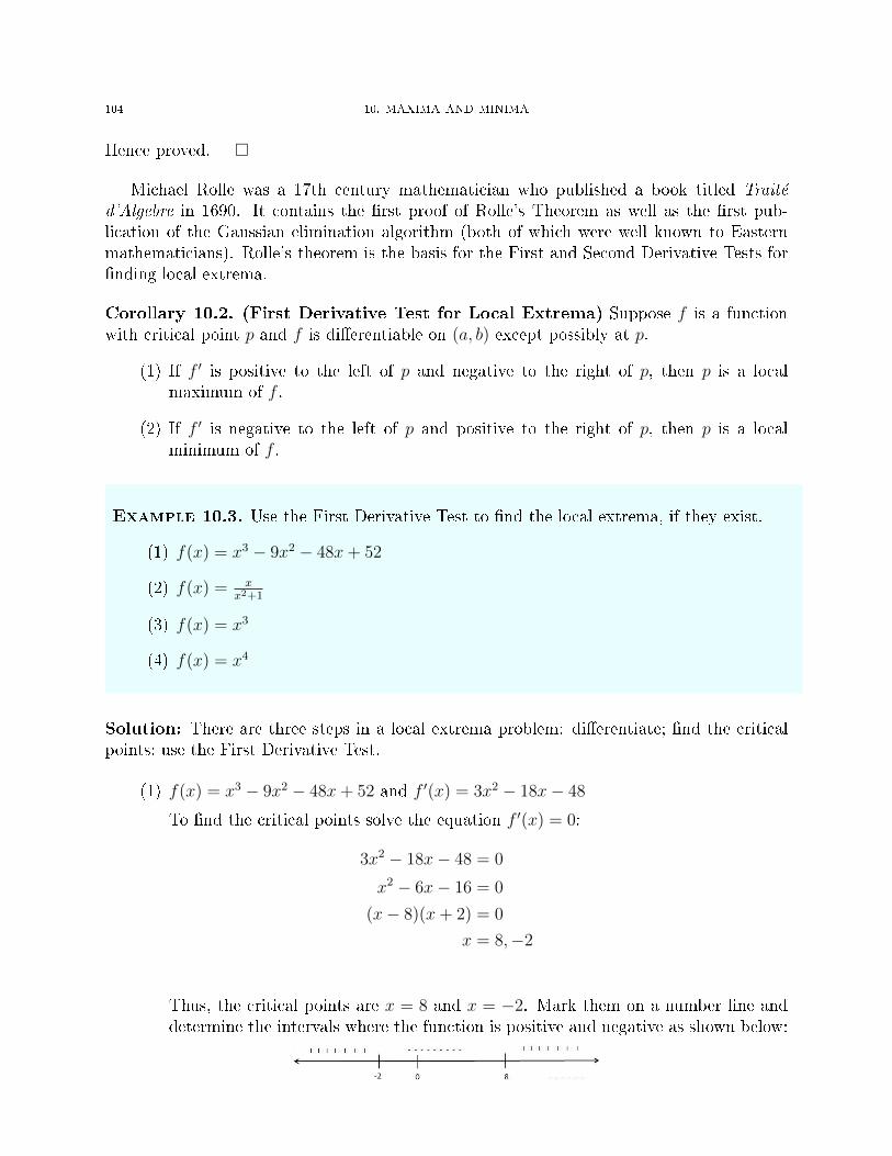
104 10. MAXIMA AND MINIMA
Hence proved. �
Michael Rolle was a 17th century mathematician who published a book titled Traité
d'Algebre in 1690. It contains the �rst proof of Rolle's Theorem as well as the �rst pub-lication of the Gaussian elimination algorithm (both of which were well known to Easternmathematicians). Rolle's theorem is the basis for the First and Second Derivative Tests for�nding local extrema.
Corollary 10.2. (First Derivative Test for Local Extrema) Suppose f is a functionwith critical point p and f is di�erentiable on (a, b) except possibly at p.
(1) If f ′ is positive to the left of p and negative to the right of p, then p is a localmaximum of f .
(2) If f ′ is negative to the left of p and positive to the right of p, then p is a localminimum of f .
Example 10.3. Use the First Derivative Test to �nd the local extrema, if they exist.
(1) f(x) = x3 − 9x2 − 48x+ 52
(2) f(x) = xx2+1
(3) f(x) = x3
(4) f(x) = x4
Solution: There are three steps in a local extrema problem: di�erentiate; �nd the criticalpoints; use the First Derivative Test.
(1) f(x) = x3 − 9x2 − 48x+ 52 and f ′(x) = 3x2 − 18x− 48
To �nd the critical points solve the equation f ′(x) = 0:
3x2 − 18x− 48 = 0
x2 − 6x− 16 = 0
(x− 8)(x+ 2) = 0
x = 8,−2
Thus, the critical points are x = 8 and x = −2. Mark them on a number line anddetermine the intervals where the function is positive and negative as shown below:

10. MAXIMA AND MINIMA 105
Since f ′ is positive to the left of -2 and negative to the right of -2, a local maximumoccurs at −2. The value of the local maximum is
f(−2) = (−2)3 − 9(−2)2 − 48(−2) + 52 = 104.
Since f ′ is negative to the left of 8 and positive to the right of 8, a local minimumoccurs at 8. The value of the local minimum is
f(8) = (8)3 − 9(8)2 − 48(8) + 52 = −396.
(Note that once the technique is mastered the problem can be solved with fewerwords.)
(2)
f(x) =x
x2 + 1
f ′(x) =1− x2
(x2 + 1)2
Critical Points:
1− x2 = 0
x = ±1
Since f ′ is positive to the left of -1 and negative to the right of -1, a local maximumoccurs at −1. The value of the local maximum is
f(−1) = −1
2.
Since f ′ is negative to the left of 1 and positive to the right of 1, a local minimumoccurs at 1. The value of the local minimum is
f(1) =1
2.
(3)f(x) = x3
f ′(x) = 3x2
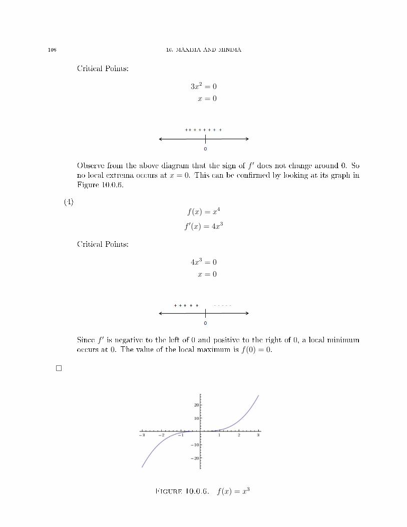
106 10. MAXIMA AND MINIMA
Critical Points:
3x2 = 0
x = 0
Observe from the above diagram that the sign of f ′ does not change around 0. Sono local extrema occurs at x = 0. This can be con�rmed by looking at its graph inFigure 10.0.6.
(4)f(x) = x4
f ′(x) = 4x3
Critical Points:
4x3 = 0
x = 0
Since f ′ is negative to the left of 0 and positive to the right of 0, a local minimumoccurs at 0. The value of the local maximum is f(0) = 0.
�
Figure 10.0.6. f(x) = x3
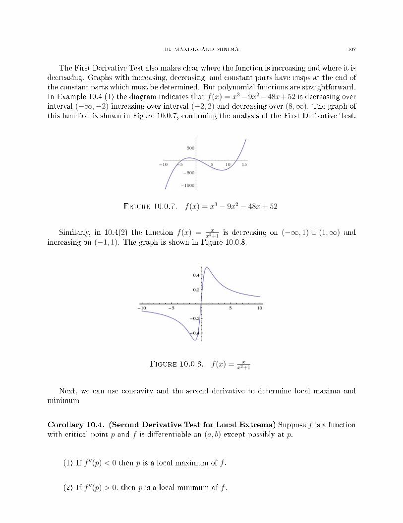
10. MAXIMA AND MINIMA 107
The First Derivative Test also makes clear where the function is increasing and where it isdecreasing. Graphs with increasing, decreasing, and constant parts have cusps at the end ofthe constant parts which must be determined. But polynomial functions are straightforward.In Example 10.4 (1) the diagram indicates that f(x) = x3−9x2−48x+52 is decreasing overinterval (−∞,−2) increasing over interval (−2, 2) and decreasing over (8,∞). The graph ofthis function is shown in Figure 10.0.7, con�rming the analysis of the First Derivative Test.
Figure 10.0.7. f(x) = x3 − 9x2 − 48x+ 52
Similarly, in 10.4(2) the function f(x) = xx2+1
is decreasing on (−∞, 1) ∪ (1,∞) andincreasing on (−1, 1). The graph is shown in Figure 10.0.8.
Figure 10.0.8. f(x) = xx2+1
Next, we can use concavity and the second derivative to determine local maxima andminimum
Corollary 10.4. (Second Derivative Test for Local Extrema) Suppose f is a functionwith critical point p and f is di�erentiable on (a, b) except possibly at p.
(1) If f ′′(p) < 0 then p is a local maximum of f .
(2) If f ′′(p) > 0, then p is a local minimum of f .

108 10. MAXIMA AND MINIMA
Example 10.5. Find the local extrema, if they exist. Use the second derivative test.
(1) f(x) = x3 − 9x2 − 48x+ 52
(2) f(x) = xe−x
(3) f(x) = x+ 1x
Solutions.
(1) f(x) = x3 − 9x2 − 48x+ 52
As we saw in the previous example, f ′(x) = 3x2 − 18x − 48 and f ′′(x) = 6x − 18and f has critical points at x = −2 and x = 8.
Applying the Second Derivative Test, since f ′′(−2) = −30 < 0, f has a localmaximum at −2. Since f ′′(8) = 30 > 0, so f has a local minimum at 8.
(2) f(x) = xe−x
f ′(x) = e−x − xe−x = e−x(1− x)
f ′′(x) = −e−x(1− x)− e−x = e−x(x− 2)
To �nd the critical points set e−x(1− x) = 0 and solve for x. Since the exponentialfunction is never 0, the only way e−x(1− x) can be 0 is when 1− x = 0. So x = 1.Thus f has a critical point at x = 1. Applying the Second Derivative Test, sincef ′′(1) = −e−1 < 0, f has a local maximum at 1.
(3) f(x) = x+ 1x
f ′(x) = 1− 1
x2
f ′′(x) =2
x3
Critical Points:
1− 1
x2= 0
1
x2= 1
x2 = 1
x = ±1
So f has critical points at x = ±1. Applying the Second Derivative Test, sincef ′′(−1) < 0, f has a local maximum at −1. Since f ′′(1) > 0, f has a local minimumat 1.

10. MAXIMA AND MINIMA 109
�
Arguably the Second Derivative Test is faster to use than the First Derivative Test, butonly when the second derivative is easy to �nd and it doesn't always work. For example,consider the function
f(x) = x4
whose local minimal was found to be x = 0 using the First Derivative Test. Observe thatf ′(x) = 4x3 and f has a critical point at x = 0. However, f ′′(x) = 12x2 so f ′′(0) = 0.In this case, the Second Derivative Test failed. The First Derivative Test always works.Moreover, the First Derivative Test also clearly indicates the intervals over which the functionis increasing and decreasing as explained earlier.
Corollary 10.6. (Test for concavity) Suppose f is a function di�erentiable on an openinterval (a, b) containing c and suppose f ′′(c) exists.
(1) If f ′′(c) > 0, then f ′(x) is increasing at c, and f is concave up at c.
(2) If f ′′(c) is negative, then f ′(x) is decreasing at c, and f is concave down at c.
De�nition: An in�ection point is a point on a curve at which a change in the directionof curvature occurs. (The concavity changes.)
Observe that the tangent line to the curve at a point is above the curve for the concavedown portion (or convex portion) and below the curve for the concave up portion. Thein�ection point is where it moves from one side to the other. 1 It can be di�cult todetermine concavity just by looking at the graph, especially if the concavity is slight. TheTest for Concavity gives a precise way of �nding the in�ection points.
Theorem 10.7. (Test for in�ection points) Suppose f is a function di�erentiable on anopen interval (a, b) containing k and suppose f ′′(k) = 0. Then k is an in�ection point if andonly if f ′′ changes signs around k.
Example 10.8. Find the in�ection points, if they exist.
(1) f(x) = x3
(2) f(x) = x3 − 9x2 − 48x+ 52
(3) f(x) = x4 − x
Solutions. We will �nd the �rst and second derivatives and use the Test for Infection points.
1The Wikipedia page for �In�ection Points" has an animated gif showing how the tangent line to thecurve changes from one side of the curve to the other at the in�ection point.
110 10. MAXIMA AND MINIMA
(1) Observe that
f(x) = x3
f ′(x) = 3x2
f ′′(x) = 6x
Candidates for in�ection points are obtained by setting f ′′(x) = 0 and solving.
6x = 0
x = 0
From the diagram above, observe that f ′′ is negative to the left of 0 and positive tothe right of 0. Since the sign of f ′′ changes using the Test for In�ection Points, wecans ay an in�ection point occurs at 0. The infection point is (0, 0).
(2)
f(x) = x3 − 9x2 − 48x+ 52
f ′(x) = 3x2 − 18x− 48
f ′′(x) = 6x− 18
Candidates for infection points:
6x− 18 = 0
x = 3
From the diagram above, since the sign of f ′′ changes about x = 3, an in�ectionpoint occurs at 3. The infection point is (3, f(3)).
(3)
f(x) = x4 − xf ′(x) = 4x3 − 1
f ′′(x) = 12x2
Candidates for infection points:
f ′′(x) = 0
12x2 = 0
x = 0
However, f ′′ does not change sign around x = 0. So x = 0 is not an in�ection point.This function has no in�ection point. See the graph of f(x) = x4 − x in Figure10.0.9.

10. MAXIMA AND MINIMA 111
Figure 10.0.9. f(x) = x4 − x
�
Finding the intervals over which the function is increasing and decreasing, the localextrema, and the in�ection points helps in drawing a good graph. For example take a lookat the graph of f(x) = x3 in Figure 10.0.6 and observe the way the curvature changes atx = 0. In fact, have you ever wondered why f(x) = x3 looks the way it does? After allwe plot by hand just a few points and even though the computer can plot a point for everypixel, it is still just plotting points. There are in�nite real numbers between every pair ofreal numbers, so how do we know something strange does not occur at points to �ne to plot.The shape of the graph is governed by the local extrema and in�ection points.
Practice Problems
(1) For each function �nd the following, if they exist:
i) The critical points
ii) The local extrema using the �rst derivative test
iii) The intervals over which the function is increasing and decreasing
iv) The local extrema using the second derivative test (if possible)
v) The in�ection points
a) f(x) = 5x2 + 4x
b) f(x) = 3x2 − 12x+ 5
c) f(x) = (x2 − 1)3
d) f(x) = x3 + 3x2 − 24x
e) f(x) = x3 + x2 − xf) f(x) = 3x4 + 3x3 − 6x2
112 10. MAXIMA AND MINIMA
g) f(x) = |3x− 4|h) f(x) = x
x2+1
i) f(x) = x−1x2−x+1
j) f(x) = x−1x2+4
k) f(x) =√
1− x2
l) f(x) = x2e−3x
m) f(x) = lnxx2

CHAPTER 11
Optimization
In this chapter we take our new found ability to �nd the maximum and minimum offunctions and apply it to all sorts of real world situations. As Euler said
Since the fabric of the universe is most perfect and the work of a most wiseCreator, nothing at all takes place in the universe in which some rule ofmaximum or minimum does not appear.
We now know the universe is not as predictable as the golden age mathematicians believed itto be. Nonetheless, many real world phenomena can be reduced to a local extrema problem.
Example 11.1. (Maximizing Area) A farmer has 2400 feet of fence and he wants tofence o� a rectangular �eld that borders a straight river. He needs no fence along the river.What are the dimensions of the �eld that has the largest area?
Solution. Suppose l is the length and w is the width of the �eld. The area A of the �eld is
A = lw
and the perimeter P isP = 2w + l
since one side is not fenced (it could be l or w that appears once).
The problem speci�es that the perimeter is �xed at 2400, which is the amount of fencethe farmer has. Using the perimeter formula we get
P = 2w + l
2400 = 2w + l
l = 2400− 2w.
Substitute the value of l in the area formula to get
A = lw = (2400− 2w)w = 2400w − 2w2.
113

114 11. OPTIMIZATION
Since the problem asks for the largest area, the function to maximize is A = 2400w−2w2. Wecan use the First Derivative Test or Second Derivative Test. Let's try the Second DerivativeTest since it is shorter. The derivative is
A′ = 2400− 4w.
The critical point is
A′ = 0
2400− 4w = 0
−4w = 2400
w = 600.
The second derivative isA′′ = −4.
Since the second derivative is negative, A has a maximum at
w = 600.
The corresponding value of l is
l = 2400− 2w = 2400− 2(600) = 1200.
Therefore, the �eld with the largest area has w = 600 feet and l = 1200 feet. �
Example 11.2. (Maximizing Volume) An open box having a square base and a surfacearea of 108 square inches must be constructed. What dimensions will produce a box withmaximum volume?
Solution: Suppose the box has a square base of length x and height h. The volume of thebox is
V = x2h
and the surface area isS = x2 + 4xh.

11. OPTIMIZATION 115
The problem speci�es that the surface area is �xed at 108 square inches. Using thesurface area formula
S = x2 + 4xh
108 = x2 + 4xh
108− x2 = 4xh
h =108− x2
4x.
Substitute the value of h in the volume formula to get
V = x2h = x2(
108− x2
4x
)= 27x− x3
4.
The �rst and second derivatives are
V ′ = 27− 3
4x2
V ′′ = −3
2x
The critical points are
V ′ = 0
27− 3
4x2 = 0
3
4x2 = 27
x2 = 36
x = ±6.
Using the second derivative test, V ′ is negative at x = 6. So V is maximum at
x = 6.
The corresponding value of h is
h =108− 36
36= 2.
Therefore the dimensions giving the maximum volume are x = 6 inches and h = 2 inches.�
Example 11.3. (Maximizing Surface Area) A cylindrical can must be constructedto hold 1000 cubic centimeters of oil. Find the dimensions that minimize the cost of thematerials needed to manufacture the can.

116 11. OPTIMIZATION
Solution: Suppose the radius of the can's base is r and height is h. Volume of the can is
V = πr2h.
The surface area of the can is the area of the top and bottom circles which is 2 × πr2 andthe area of the cylinderical part. This portion unfolds to a rectangle with one side h and theother side 2πr, so its area is 2πr × h. Thus the surface area of a cylinderical can is
S = 2πr2 + 2πrh.
The problem speci�es that the volume is �xed at 1000 cubic centimeters. So
1000 = πr2h
h =1000
πr2.
Substitute h is the surface area formula to get
S = 2πr(r +1000
πr2) = 2πr2 +
2000
r.
The �rst and second derivatives are
S ′ = 4πr − 2000
r2
S ′′ = 4π +4000
r3.
The critical points are obtained by setting
S ′ = 0
4πr − 2000
r2= 0
4πr3 − 2000
r2= 0
11. OPTIMIZATION 117
Setting the numerator zero gives
4πr3 − 2000 = 0
r3 =500
π
r =3
√500
π≈ 5.42.
So the critical point is r = 5.42. 1 Using the Second Derivative Test, observe that A′′ ispositive at r ≈ 5.42. So V is minimum at
r ≈ 5.42.
The corresponding value of h is
h =1000
π3√
5.422≈ 10.84.
Therefore, the dimensions of the can that minimize the surface area (and therefore the costof materials) is r ≈ 5.42 cm and h ≈ 10.84 cm. 2
Example 11.4. A rectangular page must be constructed with 24 square inches of print,with top and bottom margins of 1.5 inches and left and right margins of 1 inch. What shouldthe dimensions of the page be in order to use the least amount of paper?
Solution: Suppose the printed portion has length l and width w. The area of the printedportion is given as 24. So
24 = lw
w =24
l.
1Note that 4πr3−2000r2 = 0 is a rational equation which is zero when the numerator is zero. The numerator
is the cubic equation 4πr3 − 2000. It has one real root and two complex roots. But r cannot be a complex
number so we disregard the complex roots. Further, note that 4πr3−2000r2 = 0 is unde�ned at r = 0 making
it another critical point. But a solution with r = 0 would not make sense, so we can disregard it. Thesereasons must be known for a thorough understanding, even if forgetting them and �nding only the real rootgets you to the �nal answer.
2 See http://samjshah.com/2012/05/31/a-calculus-optimization-poster-project/ for a Calculus Opti-mization project where students can implement this analysis for various grocery items such as soup cans,soda cans etc. to determine how �volume optimized� the cans are.

118 11. OPTIMIZATION
Since the left and right margins are 1 inch each, the length of the printed portion is l− 2and since the top and bottom margins are 1.5 inches each, the width is w − 2. The area ofthe page is
A = (l + 2)(w + 3).
Substituting the value of w in the above formula gives
A = (l + 2)(24
l+ 3) = 30 + 2l +
72
l
The �rst and second derivatives are
A′ = 2− 72
l2
andA′′ =
144
x3.
The critical points are
2− 72
l2= 0
2l2 = 72
l2 = 36
l = ±6.
Since a solution with l = −6 doesn't make sense, we may assume l = 6. Since A′ is positivewhen l = 6, by the Second Derivative Test A′ is minimized at
l = 6.
The corresponding w value is
w =24
l= 4.
Therefore, the dimensions of the printed area using the least paper are l = 6 inches andw = 4 inches. �
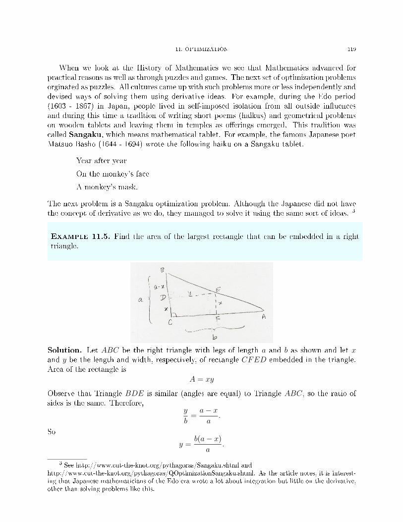
11. OPTIMIZATION 119
When we look at the History of Mathematics we see that Mathematics advanced forpractical reasons as well as through puzzles and games. The next set of optimization problemsorginated as puzzles. All cultures came up with such problems more or less independently anddevised ways of solving them using derivative ideas. For example, during the Edo period(1603 - 1867) in Japan, people lived in self-imposed isolation from all outside in�uencesand during this time a tradition of writing short poems (haikus) and geometrical problemson wooden tablets and leaving them in temples as o�erings emerged. This tradition wascalled Sangaku, which means mathematical tablet. For example, the famous Japanese poetMatsuo Basho (1644 - 1694) wrote the following haiku on a Sangaku tablet.
Year after year
On the monkey's face
A monkey's mask.
The next problem is a Sangaku optimization problem. Although the Japanese did not havethe concept of derivative as we do, they managed to solve it using the same sort of ideas. 3
Example 11.5. Find the area of the largest rectangle that can be embedded in a righttriangle.
Solution. Let ABC be the right triangle with legs of length a and b as shown and let xand y be the length and width, respectively, of rectangle CFED embedded in the triangle.Area of the rectangle is
A = xy
Observe that Triangle BDE is similar (angles are equal) to Triangle ABC, so the ratio ofsides is the same. Therefore,
y
b=a− xa
.
So
y =b(a− x)
a.
3 See http://www.cut-the-knot.org/pythagoras/Sangaku.shtml andhttp://www.cut-the-knot.org/pythagoras/QOptimizationSangaku.shtml. As the article notes, it is interest-ing that Japanese mathematicians of the Edo era wrote a lot about integration but little on the derivative,other than solving problems like this.

120 11. OPTIMIZATION
Substituting the value of y in the area formula gives
A =x
y= x
b(a− x)
a=b
a(ax− x2).
The �rst and second derivatives are
A′ =b
a(a− 2x)
and
A′′ = −2b
aThe critical point is
A′ = 0
b
a(a− 2x) = 0
a− 2x = 0
2x = a
x =a
2
Since A′′ is always negative (a and b are lengths and therefore positive), by the SecondDerivative Test, x = a
2is a local maximum. So A is maximized at
x =a
2
and the corresponding value of y is
y =b
a(a− a
2) =
b
2.
Therefore, the area of the largest rectangle is ab4.
Example 11.6. Find the area of the largest rectangle that can be inscribed in a semi-circleof radius r.
Solution: Draw a circle centered at (0, 0) and radius r and inscribe a rectangle in it asshown. The rectangle has length 2x and width y.
11. OPTIMIZATION 121
The area of the rectangle isA = 2xy.
The equation of the circle isx2 + y2 = r2.
Since the point (x, y) lies on the circle (as shown)
x2 + y2 = r2
y =√r2 − x2
Substituting, the value of y in the area formula gives
A = 2xy = 2x√r2 − x2
The �rst and second derivatives are
A′ = 2
[x
1
2√r2 − x2
(−2x) +√r2 − x2
]= 2
[−x2√r2 − x2
−√r2 − x2
]= 2
[−x2 + r2 − x2√
r2 − x2
]=
2(r2 − 2x2)√r2 − x2
=2r2 − 4x2√r2 − x2
and
A′′ =1
r2 − x2
[√r2 − x2(−8x)− (2r2 − 4x2)
−2x
2√r2 − x2
]=
1
(r2 − x2) 32
[(r2 − x2)(−8x)− (2r2 − 4x2)(−x)
]=
1
(r2 − x2) 32
[−8xr2 + 8x3 + 2xr2 − 4x3
]=
1
(r2 − x2) 32
[−6xr2 + 4x3
]
The critical points are the points where A′ is unde�ned or 0. Observe that A′ is unde�nedwhen x = ±r, but it makes no sense geometrically, so we disregard it. Setting the numerator
122 11. OPTIMIZATION
equal to zero gives
2(r2 − 2x2) = 0
x = ± r√2
Observe that when x = r√2the value of A′
A′ =1
(r2 − r2
2)32
[−6
r√2r2 + 4
r3
8
]=
1
r3
[− 6√
2r3 +
r3
2
]=
1
r3√
2(−11r3)
Since A′ is negative when r√2, by the Second Derivative Test, it is a local maximum. So A
is maximized whenx =
r√2
and the corresponding y value is
y =
√r2 −
(r√2
)2
=r√2.
The area of the largest rectangle is
A =2r√
2
r√2
= r2
�
The di�erentiation in the above problem would have been easier if we were given a speci�cvalue of r. In the next two problems we reduce the generality of the question by talkingabout speci�c geometrical objects and speci�c points.
Example 11.7. Find the point on the line y = 4x+ 7 that is closest to the origin (0, 0).
Solution: Let (x, y) be a point on the line y = 4x+ 7 and let d be the distance from (x, y)to the origin (0, 0).
d =√
(x− 0)2 + (y − 0)2 =√x2 + y2.
It would be di�cult to maximize d, so we maximize d2. (This portion is not obvious and isexplained in further detail after the solution.) Substitute the value of y = 4x+ 7 to get
d2 = x2 + (4x+ 7)2 = x2 + 16x2 + 56x+ 49 = 17x2 + 56x+ 49

11. OPTIMIZATION 123
For the purpose of applying the Second Derivative Test let us call this function
f(x) = 17x2 + 56x+ 49
f ′(x) = 34x+ 56
The critical point is x = −5634≈ −1.65. Since the second derivative is f ′′(x) = 34, which
is positive, x = −1.64 is a minimum. The corresponding y is y = 4x + 7 = 0.41. Thereforethe point on the graph closest to the origin is (−1.65, 0.4). �
Now let us understand in more detail why we can naximize d2 in place of d in the aboveproblem. Intuitively, consider an increasing function f and let g = f 2. Then g is also anincreasing function. So f and g will have the same local extrema. Formally, a functionf is strictly increasing on an interval [a, b] if, for any x1, x2 ∈ [a, b] such that x1 < x2,f(x1) < f(x2).
Theorem 11.8. Suppose f is a di�erentiable function on an interval [a, b] and that g is adi�erentiable, strictly increasing function on the interval [f(a), f(b)]. Let h = g ◦ f , that ish(x) = g(f(x)). Then the local maxima and minima of h are the same as the local maximaand minima of f , respectively.
Proof. Suppose c is a local maximum of f . By de�nition of local maximum for some interval(d, e) containing c,
f(x) < f(c)
for all x ∈ (d, e) distinct from c. Since g is strictly increasing,
g(f(x)) < g(f(c)).
Therefore c is a local maximum for g ◦ f .Similarly, if c is a local minimum of f , then c must also be a local minimum for h. �
Example 11.9. Find the point on the parabola x = y2
2that is closest to the point (1, 4).
Solution: Let (x, y) be a point on the parabola x = y2
2and let f be the square of the
distance of (x, y) from x = y2
2. Observe that
f = (x− 1)2 + (y − 4)2
and replacing x = y2
2gives
f = (1
2y2 − 1)2 + (y − 4)2.

124 11. OPTIMIZATION
The �rst and second derivatives are
f ′ = 2(1
2y2 − 1)y + 2(y − 4) = y3 − 2y + 2y − 8 = y3 − 8
f ′′ = 3y2
The real root of y3 − 8 = 0 is y = 2. So f has a critical point at y = 2. Since f ′′ is positivewhen y = 2, by the Second Derivative Test, y = 2 is a local minimum. So f is minimizedby y = 2 and the corresponding value of x is x = y2
2= 22
2= 2. Therefore the point on the
parabola closest to (1, 2) is (2, 2).
Example 11.10. Find the points on the ellipse 4x2 + y2 = 4 farthest from (1, 0).
Solution: Let (x, y) be a point on the ellipse and let f be the square of the distance from(x, y) to (1, 0). Then
f = (x− 1)2 + y2.
Using the equation of the ellipse, we can write y2 = 4− 4x2, so we can substitute in f toobtain
f = (x− 1)2 + 4− 4x2 = 5− 2x− 3x2
The �rst and second derivatives are
f ′′ = −2− 6x
f ′′(x) = −6.
The critical point is x = −13. Since f ′′ is negative, x = −1
3is a local maximum. The
corresponding y values are
±
√4− 4
(1
9
)= ±
√32
9= ±4
√2
3.
Therefore, the farthest points from (1, 0) on the ellipse are (−13,±4
√2
3). �
Practice Problems

11. OPTIMIZATION 125
(1) Find two positive numbers that satisfy the following constraints:
a) The sum is 100 with maximum product
b) the product is 192 with maximum sum
c) The product is 192 and the sum of the �rst plus three times the second is aminimum
d) The sum of the �rst and twice the second is 100 with maximum product
(2) A farmer as 2400 meters of fencing and wants to fence o� a rectangular �eld thatborders a straight river. He needs no fence along the river. What are the dimensionsof the �eld that has the largest area?
(3) A farmer wants to fence a rectangular pasture adjacent to a river. The pasture mustcontain 180,000 square meters in order to provide enough grass for the herd. Whatdimensions would require the least amount of fencing if no fencing is needed alongthe river?
(4) A manufacturer wants to design an open box having a square base and surface areaof 108 square inches. What dimensions will produce a box with maximum volume?
(5) Find the dimensions of a rectangular solid with a square base of maximum volumeif the surface area is 160 square inches.
(6) A rectangular page has 24 square inches of print. Margins at the top and bottomare 1.5 inches and on the left and right are 1 inch What should the dimensions ofthe page be so that the smallest number of pages are used?
(7) A rectangular page is to contain 30 square inches of print. The margins on each sideare 1 inch. Find the dimensions of the page so that the smallest amount of paper isused.
(8) A cylindrical can is to be made to hold 1000 cubic centimeters of oil. Find thedimensions that minimize the cost of the metal to manufacture the can.
(9) Find the point on the parabola y2 = 2x that is closest to the point (1, 4).
(10) Find the area of the largest rectangle that can be inscribed in a semi-circle of radiusr.
(11) A rectangular box with a square base and no top is to have a volume of 108 cubicinches. Find the dimensions of the box that require the smallest amount of material.