DOE/ID-10844 March 2001

Calendar-Life Studies of Advanced Technology Development Program Gen 1 Lithium Ion Batteries

This report was prepared as an account of work sponsored by an agency of the United States Government. Neither the United States Government nor any agency thereof, nor any of their employees, make any warranty, express or implied, or assumes any legal liability or responsibility for the accuracy, completeness, or usefulness of any information, apparatus, product or process disclosed, or represents that its use would not infringe on privately owned rights. References herein to any specific commercial product, process, or service by trade name, trademark, manufacturer, or otherwise, does not necessarily constitute or imply its endorsement, recommendation, or favoring by the United States Government or any agency thereof. The views and opinions of authors expressed herein do not necessarily state or reflect those of the United States Government or any agency thereof.

DOE/ID-10844

Calendar-Life Studies of Advanced Technology Development Program Gen 1 Lithium Ion Batteries

Randy B. Wright Chester G. Motloch

Published March 2001

Prepared for the U.S. Department of Energy

Assistant Secretary for Energy Efficiency and Renewable Energy (EE) Idaho Operations Office

ii

ABSTRACT

This report presents the test results of a special calendar-life test conducted on 18650-size, prototype, lithium-ion battery cells developed to establish a baseline chemistry and performance for the Advanced Technology Development Program. As part of electrical performance testing, a new calendar-life test protocol was used. The test consisted of a once-per-day discharge and charge pulse designed to have minimal impact on the cell yet establish the performance of the cell over a period of time such that the calendar life of the cell could be determined. The calendar life test matrix included two states of charge (i.e., 60 and 80%) and four temperatures (40, 50, 60, and 70ºC). Discharge and regen resistances were calculated from the test data. Results indicate that both discharge and regen resistance increased nonlinearly as a function of the test time. The magnitude of the discharge and regen resistance depended on the temperature and state of charge at which the test was conducted. The calculated discharge and regen resistances were then used to develop empirical models that may be useful to predict the calendar life of the cells.

iii

iv

EXECUTIVE SUMMARY

The DOE Office of Advanced Automotive Technologies, through the Partnership for a New Generation of Vehicles (PNGV) Advanced Energy Technology Development (ATD) Program, is engaged in the study of 18650-size lithium-ion cells, which baseline the high-power battery chemistry being developed for use in hybrid electric vehicles (HEVs). The cells received for testing were built by a commercial vendor to specifications supplied by the ATD program. These cells contain cathodes of 84 wt% LiNi0.8Co0.2O2, with graphite and carbon black added for electrical conductivity. The anode is a blend of SFG-6 and MCMB-6 carbons. The electrolyte is 1.0 M LiPF6 in 1:1 EC/DEC (ethylene carbonate:diethyl carbonate = 1:1). PVDF [polyvinylidene fluoride, (-CH2-CF2-)n] binder was used in the fabrication of both electrodes. The anode current collector is copper foil; the cathode current collector is aluminum foil. Celgard supplied the separator (polyethylene). The cells, as part of their electrical performance testing, were tested using a new test protocol developed by the ATD program to test calendar-life.

This report presents the test results pertaining to this group of prototype lithium ion batteries. The cells had a nominal capacity of 0.9 A·h at a C/1 discharge rate with a voltage range of 3 to 4.1 V. The cells were assembled into a 18650-size container (64.9 mm high, 18.1 mm diameter). The cells underwent a number of electrical performance tests to determine their electrochemical performance at 25oC. A special calendar-life test was also conducted at elevated temperatures of 40, 50, 60, and 70oC.

The specific test for which the data are presented and discussed in this report was a special calendar-life test conducted once per day for a period of time depending on the test temperature. This test, consisting of specified discharge and charge protocols, was specially designed to have a minimal impact on the cell yet establish the performance of the cell over a period of time such that the calendar life of the cell could be determined. Specific discharge and regen current levels at specific time duration were used at each once-per-day test cycle. The calendar-life test was conducted at 60 and 80% state of charge (SOC). During the calendar-life test, the discharge resistance was determined from the discharge portion of the test; the regen resistance was determined from the regen portion of the test.

The results of the testing indicate that both the discharge and regen resistance increased nonlinearly as a function of the test time. The magnitude of the discharge and regen resistance depended on the temperature and SOC at which the test was conducted. General observations derived from this study are as follows:

1. Both the discharge and regen resistances have a nonlinear increase with respect to time at test temperature.

2. The discharge resistances are greater than the regen resistances at all of the test temperatures of 40, 50, 60, and 70oC.

v

3. For both the discharge and regen resistances, generally the higher the test temperature, the lower the resistance.

4. The 70oC discharge and regen resistance data at 80% SOC do not follow the general trend of the rest of the data in that the resistance at this temperature is slightly greater than that at 60oC. At 60% SOC, the discharge and regen resistance data indicate that a process is occurring that causes the 60oC resistance to be greater than at 50oC. The 70oC data may also be influenced at this SOC. These observations appear to indicate that new physical/chemical processes are occurring that causes an anomalous increase in the resistance. They also indicate that the state of charge at which the test was conducted may influence the temperature at which the onset of these new processes occurs. The exact nature of these processes is not presently known.

5. Both the discharge and regen resistance are greater at 80% SOC than they are at 60% SOC.

6. There are also differences in the rate of increase of the resistances in that the 80% SOC resistance increases faster than at 60% SOC.

A model was developed to account for the time, temperature, and SOC of the batteries during the calendar-life test. The functional form of the model is given by

R(t,T,SOC) = A(T,SOC)F(t) + B(T,SOC)

where t is the time at test temperature, T is the test temperature, and SOC is the state of charge of the cell at the start of the test. A and B are assumed to be functions of the temperature and state of charge; F is assumed to be only a function of the time at test temperature. Using curve fitting techniques for a number of time-dependent functions, it was found that both the discharge and regen resistance were best correlated by a square root of time dependence. These results led to the relationship for the discharge and regen resistance:

R(t,T,SOC) = A(T,SOC)t1/2 + B(T,SOC) .

The square root of time dependence can be accounted for by either a one-dimensional diffusion type of mechanism, presumably of the lithium ions, or by a parabolic growth mechanism for the growth of a thin-film solid electrolyte interface (SEI) layer on the anode and/or cathode. The diffusion type of mechanism would arise from the lithium ions diffusing into or out of the electrodes, through the electrolyte, through the separator, or through the SEI present on the surface of the electrode materials. The growth of a thin film mechanism could be related to the growth of an SEI layer on the anode and/or cathode as a function of test time. The increased thickness of the SEI film would increase the resistance of the cell due to increased hindrance of the transport of lithium ions through the SEI layer to subsequently be intercalated/de-intercalated into the active electrode material. The best physical/chemical model appears at present to be the growth of the SEI layer. The present data, however, cannot determine if the growth of the SEI layer with time occurs at the anode, the

vi

cathode, or both. There are characterization/diagnostic results, in particular electrochemical impedance spectroscopic (EIS) methods, that indicate that the resistance of the cathode is the major contributor to the resistance of the cell as it ages. The temperature dependence of the resistance was then investigated using various model fits to the functions A(T) and B(T). The results of this exercise lead to a functional form for the temperature dependence of the fitting functions having an “Arrhenius-like” form:

A(T) = a[exp(b/T)] and B(T) = c[exp(d/T)]

where a and c are constants, and b and d are related to an activation energy, Eb and Ed, by using the gas constant, R, such that b = Eb/R and d = Ed/R. The values of Eb and Ed were determined and were found to be of the right order of magnitude (several to several tens of kjoules/mole) for the activated transport of lithium ions. It is not known what specific process or processes the determined activation energy values correspond too. The functional form, therefore, for the discharge and regen resistance, including the SOC, is then

R(t,T,SOC) = a(SOC){exp[b(SOC)/T]}t1/2 + c(SOC){exp[d(SOC)/T]} .

The a, b, c, and d parameters are explicitly shown as being functions of the SOC. However, due to the lack of testing at SOC values other than 60 and 80% SOC, the exact form of the SOC dependence could not be determined from the experimental data. Once the values of a, b, c, and d were determined, the function R(t,T,SOC) could then be used to correlate the discharge and regen data and to predict what the resistances would be at different times and test temperatures.

As part of the calendar-life testing, the cells underwent the calendar-life once-per-day test for a specified period of time at a specified test temperature. For test temperatures of 40, 50, and 60oC, the test time was 4 weeks. For the cells tested at 70oC, the test time was 2 weeks. The cells were then cooled to 25oC for conduct of reference performance tests. The cells were then reheated to the specified elevated test temperature, and the calendar-life test was repeated. During conduct of this second, and subsequent calendar life cyclic testing, the discharge and regen resistances were observed to slowly reach the resistance before cool down. After this previous resistance was reached, the resistance continued to increase throughout the test. The above model and one that has a logarithmic in test time at temperature dependence were applied to this resistance regrowth and were found to account for its time and temperature behavior.

Analysis of the C/1 discharge test results allowed determining the leakage current, i.e., the current required to maintain a given voltage on the cell. In this case, the cells where held constant at 4.1 V. The leakage current was found to decrease quite rapidly for new cells, but after aging due to testing, the magnitude of the leakage current as a function of test time increased. The leakage current can be related to a leakage resistance via Ohm’s law. The leakage resistance decreased as the cell aged, which means that more current, i.e., charge, has to be put into the cell to maintain a given voltage. This increased charge results from IR-losses in the battery. The IR-losses increase, due to presently unknown complex processes, as the cell ages.

vii

Further analysis of the C/1 (and C/25) charge and discharge data using the concept of differential capacitance was applied to the test data. This analysis simply takes the derivative of the charge added or removed with respect to the cell voltage, or alternatively the charge added or removed during the test. Peaks in the differential capacitance are believed to relate to intercalation sites within the anode and cathode. As the cell aged with testing, the height of the peaks changed, as did their positions with respect to the cell voltage or charge/discharge state. The exact nature of these sites, and how the testing influences them, is not presently known. This concept of differential capacitance is believed to be useful to research groups conducting characterization/ diagnostic studies on the fresh, as well as aged, cells. The usefulness arises in that it provides information regarding the voltage and state of charge at which the properties of the cell are changing the most due to use.

viii

CONTENTS

ABSTRACT....................................................................................................................................... iii

EXECUTIVE SUMMARY ............................................................................................................... v

ACKNOWLEDGMENTS ................................................................................................................. xi

1. INTRODUCTION................................................................................................................... 1

1.1 Background ................................................................................................................... 1

1.2 Purpose and Applicability ............................................................................................. 1

2. DESCRIPTION OF LITHIUM ION CELLS.......................................................................... 3

3. ELECTRICAL PERFORMANCE TESTS ............................................................................. 5

4. CALENDAR-LIFE TESTS AT 80% SOC ............................................................................. 8

4.1 Discharge Resistance .................................................................................................... 8

4.2 Regen Resistance .......................................................................................................... 17

5. CALENDAR-LIFE TESTS AT 60% SOC ............................................................................. 21

5.1 Discharge Resistance .................................................................................................... 21

5.2 Regen Resistance .......................................................................................................... 22

6. REGROWTH OF RESISTANCE AFTER THE FIRST CALENDAR-LIFE TEST CYCLE.................................................................................................................................... 25

7. EFFECT OF SOC ON THE CALENDAR-LIFE TESTS ....................................................... 27

8. LEAKAGE CURRENT, LEAKAGE RESISTANCE, AND DIFFERENTIAL CAPACITANCE OF ATD GEN 1 CELLS ............................................................................ 29

9. SUMMARY ............................................................................................................................ 35

10. REFERENCES........................................................................................................................ 38

Appendix A—Figures for Calendar-Life and Cycle-Life Discharge and Regen Resistance Tests on ATD Gen 1 Li-Ion Batteries: Experimental Electrical Performance Test Cycles

Appendix B—Figures for Calendar-Life Discharge and Regen Resistance Tests on ATD Gen 1 Li-Ion Batteries: 80% State-of-Charge

Appendix C—Figures for Calendar-Life Discharge and Regen Resistance Tests on ATD Gen 1 Li-Ion Batteries: 60% State-of-Charge

ix

Appendix D—Figures for Calendar-Life Discharge and Regen Resistance Tests on ATD Gen 1 Li-Ion Batteries: Regrowth of Resistance after the First Calendar-Life Test Cycle, and State-of-Charge Dependence of Discharge and Regen Resistance

Appendix E—Figures from Calendar-Life Discharge and Regen Resistance Tests on ATD Gen 1 Li-Ion Batteries: Leakage Current, Leakage Resistance, and Differential Capacitance

TABLES

1. Special calendar-life test pulse profile..................................................................................... 5

2. ATD cycle-life delta 3% SOC pulse profile ............................................................................ 6

3. ATD cycle-life 6% SOC pulse profile..................................................................................... 6

4. ATD cycle-life 9% SOC pulse profile..................................................................................... 7

5. Values of Eact at 80% SOC from analysis of calendar-life test data using the relationship R(t,T) = A(T)t1/2 + B(T), where A(T) = a[exp(Eact,A/RT)], and B(T) = c[exp(Eact,B/RT)]. Eact are activation energies, and a and c are preexponential constants .................................... 20

6. Values of the preexponential constants a and c at 80% SOC from analysis of calendar-life test data analysis using the relationship R(t,T) = A(T)t1/2 + B(T), where A(T) = a[exp(Eact,A/RT)], and B(T) = c[exp(Eact,B/RT)]................................................ 20

7. Values of Eact at 60% SOC from analysis of calendar-life test data using the relationship R(t,T) = A(T)t1/2 + B(T), where A(T) = a[exp(Eact,A/RT)] and B(T) = c[exp(Eact,B/RT)]. Eact are activation energies, and a and c are preexponential constants .................................................................................................................................. 24

8. Values of the preexponential constants a and c at 60% SOC from analysis of calendar-life test data using the relationship R(t,T) = A(T)t1/2 + B(T), where A(T) = a[exp(Eact,A/RT)], and B(T) = c[exp(Eact,B/RT)] .......................................................... 24

x

ACKNOWLEDGMENTS

We wish to acknowledge the assistance of various engineers/scientists at the INEEL, SNL, and ANL. Thanks are due to Chinh Ho and Roger Richardson (INEEL) for conducting the test of the batteries, and to Jeff Belt and Jon Christophersen (INEEL) for calculating the discharge and regen resistances from the experimental data. For the testing and data reduction of their allotment of cells, thanks are due to Herb Case, David Ingersol, and Terry Unkelhaeuser (SNL), and to Ira Bloom at (ANL) for helpful discussions concerning analysis and interpretation of the data.

xi

xii

Calendar-Life Studies of Advanced Technology Development Program Gen 1 Lithium Ion Batteries

1. INTRODUCTION

1.1 Background

The DOE Office of Advanced Automotive Technologies, through the PNGV Advanced Energy Technology Development Program, is engaged in the study of 18650-size lithium-ion cells, which represent the high-power battery chemistry being developed for use in hybrid electric vehicles (HEVs). Concentrating on high-power battery development, the Advanced Energy Technology Development (ATD) Program supports the PNGV, a government-industry partnership striving to develop, by 2004, a mid-size passenger vehicle capable of achieving up to three times the fuel economy of today’s vehicles, while adhering to future emissions standards and maintaining affordability, performance, safety, and comfort. The ATD Program addresses these technical challenges through five major program areas: baseline cell development, diagnostic evaluations, electrochemical improvements, advanced materials development, and low-cost packaging. The major objective of the work is to determine the causes of power fade after these cells are exposed to elevated temperatures and tested under various electrical performance evaluation tests. Another objective is to develop diagnostic analysis methods that can be used to determine the physical/chemical causes for cell degradation.

1.2 Purpose and Applicability

This report presents the electrical performance of lithium-ion cells developed for the ATD program1 during the special pulse-per-day calendar-life testing conducted at various temperatures and states of charge. All these tests were conducted either in the Energy Storage Testing (EST) Laboratory, which is part of the Transportation Technologies and Infrastructure Department at the Idaho National Engineering and Environmental Laboratory (INEEL), or at the Lithium Battery R&D Department 1521 at Sandia National Laboratory (SNL). Also, differential capacitance comparisons were based upon a C/25 constant-current discharge calibration curve provided by the Analysis and Diagnostics Laboratory within the Chemical Technology Division at Argonne National Laboratory (ANL).

The main focus of the report is to present calendar-life test data on the cells developed by the ATD program. Calendar life is of great importance, as battery systems are expected to have a lifetime of approximately ten years if they are to be a viable energy storage/source for the next generation of vehicles. Calendar life has been defined by two general statements. The USABC Electric Vehicles Battery Test Procedures Manual, Revision 22 defines calendar life as “The length of time a battery can undergo some defined operation before failing to meet its specified end-of-life criteria.” This definition is rather nebulous. The specific definition of some defined operation would need to be clarified and stipulated in the test plan for a given battery system. The PNGV Battery Test Manual, Revision 2,3 is also rather terse in its definition of calendar life: “This test is designed to permit the evaluation of cell degradation as a result of the passage of time with minimal usage. It is not a pure shelf-life test, because the cells under test are periodically subjected to reference discharges to determine the changes (if any) in their performance characteristics.” The ATD program1 has attempted to more clearly define what is meant by a calendar-life test. The calendar-life test as used in the ATD program has been designed to have a minimal impact on the cell, yet still subject the cell to a well-specified charge/discharge test sequence over a well-defined period of time.

1

The intent of testing the model lithium-ion cells developed by the ATD program is to characterize the electrical performance and to determine the calendar-life and cycle-life behavior of specially designed lithium ion cells having a nominal capacity of 0.9 A·h. The DOE Office of Advanced Automotive Technologies (OATT) sponsored the testing and with the designated ATD Program Manager also provided oversight. In general, the cells were subjected to the performance and life test procedures defined for the PNGV Program.3

Discussion of the terminology used in this report can be found in Reference 2, USABC Electric Vehicle Battery Test Procedures Manual, Revision 2, and Reference 3, PNGV Battery Test Manual, Revision 2. The entire test procedure used to test the ATD Gen 1 cells is not reproduced here inasmuch as it is given in Reference 1, PNGV Test Plan for ATD 18650 Gen 1 Lithium Ion Cells.

2

2. DESCRIPTION OF LITHIUM ION CELLS

The baseline lithium ion cells had the following specifications, as developed by Argonne National Laboratory (ANL) for the ATD program. Cells produced with these specified materials are referred to as Gen 1 cells.

Positive electrode

LiNi0.8Co0.2O2 (Sumitomo) (84 wt%)

• Electronic additive: acetylene black (4 wt%) + SFG-6 graphite (Timcal) (4 wt%)

• Binder: polyvinylidene fluoride (-CH2-CF2-)n,(PVDF), (Kureha KF-1100 (8 wt%)

Negative electrode

• Blend of MCMB-6-2800 graphite (Osaka Gas) (75 wt%), and SFG-6 (Timcal) (16 wt%)

• Binder: PVDF (Kureha C) (9 wt%)

Electrolyte

• LiPF6/EC (ethylene carbonate)+DEC (diethyl carbonate) 1:1

Separator

• polyethylene (PE) Celgard separator (37 micron thick)

Three hundred cells were built (18650-size; 64.9 mm high, 18.12 mm diameter) and shipped to various national laboratories (ANL, BNL, INEEL, LBNL, and SNL) for electrical performance testing, and physical/chemical diagnostic analysis. The cell distribution is given in the test plan.1 For the various temperature tests, controlled temperature chambers having both heating and cooling capabilities were used. Temperature control was usually ±3oC.

The ATD Gen 1 cell limits are as follows:

Discharge

Minimum discharge voltage: 3.0 V

Maximum discharge current: 2.0 A continuous; 7.2 A (8˚C) for up to an 18-s pulse; and 13.5 A (15˚C) for up to a 2-s pulse

Maximum discharge temperature: 70oC

Charge and Regen

Maximum charge/regen voltage: 4.1 V continuous; 4.3 V for up to a 2-s pulse

Maximum charge/regen current: 0.9 A continuous charge current; 12 A maximum regen current for up to a 2-s pulse

3

Maximum Charge Temperature: 40oC

Maximum Regen Temperature: 70oC

Recharge Procedure

Charge at 0.9 A (C/1) constant current rate to a voltage of 4.1 V; continue to apply a constant voltage of 4.1 V for 2.5 hr total recharge time. All recharging is to begin at 25 ± 3oC.

4

3. ELECTRICAL PERFORMANCE TESTS

Characterization tests were performed on all the cells following a pretest readiness review. The characterization tests included a C/1 static capacity test; low- and medium-current hybrid power pulse characterization (L-HPPC and M-HPPC, respectively) tests at 2.7 A and 7.2 A, respectively; and a 7-day self-discharge test at 3.660 V, which corresponds to 50% state of charge (SOC). Thermal performance tests consisting of the static capacity and low-current HPPC tests were performed on four cells at ambient temperatures of +5 and +40oC. Finally, reference performance tests (RPTs) were conducted on all cells prior to beginning the life testing. The RPTs consisted of a single C/1 constant-current discharge, one medium-current HPPC test (M-HPPC), and impedance measurements at 1 kHz at 100 and 0% SOC. The RPTs were repeated every 4 weeks for the cells at 40, 50, and 60oC, and every 2 weeks for the cells at 70oC.

This report will deal with the calendar-life testing of these cells using a special test developed by the ATD Program. The special calendar-life test is theoretically charge-neutral, so it will not perturb the SOC of the cell any more than absolutely necessary. The magnitude and duration of the test discharge and regen are relatively modest, compared with the corresponding M-HPPC test profile, so it will have minimal effect on the thermal condition of the cell under test. [The magnitude and duration of the discharge pulse for this test (i.e., 3.6 A for 9 s) was set to one-half the corresponding values used for the M-HPPC test.] The test incorporated a somewhat longer-than-normal rest period after the discharge pulse to allow additional time for voltage recovery before the regen pulse. The calendar-life test profile is shown in Table 1 and Figure 1 (see Appendix A). Note that positive values for the current correspond to a constant current discharge.

Each cell tested using the calendar-life test was assigned a temperature and target state of charge, SOC, (either 60 or 80% SOC in this study). The determination of the voltage at a given SOC was determined from a calibration table provided by ANL that showed the voltage at a given SOC, as found by conducting C/25 discharges on a number of test cells. The discharge and regen resistances were calculated using R = ∆V/∆I, i.e., the change of the voltage of the cell at the beginning of the discharge (or charge) to the end of the discharge (or charge) divided by the change in the current during the discharge (or charge). For the calendar-life tests (see Figure 1 and Table 1), the discharge was held constant, but the voltage did change during the course of the discharge or recharge. The test was conducted once per day for a 4-week period for the 40, 50, and 60oC tests, and for a 2-week period for the 70oC test. This is a new calendar-life test designed to obtain additional resistance data at regular intervals without unduly cycling the cells. The idea was to apply a single-pulse profile once per day from which the discharge and regen resistances could be calculated.

Table 1. Special calendar-life test pulse profile.

Step Time (s)

Cumulative Time

(s)

Current

(A)

Charge (A·s)

Cumulative Charge (A·s)

9 9 3.6 32.40 32.40

60 69 0.0 0.00 32.40

2 71 -3.6 -7.20 25.20

2 73 0 0 25.20

47 120 -0.54 25.38 0.18

5

Restating the test sequence: Reference Performance Tests (RPTs) at 25 ± 3oC were conducted on all cells designated for testing, using the calendar- and cycle-life tests, and periodically during life testing. Each set of RPTs consisted of a single C/1 constant current discharge, a medium-current HPPC test, and impedance measurements at 1 kHz at 100 and 0% SOC. Cells undergoing life testing at 40, 50, and 60oC underwent RPTs every four weeks. Cells undergoing life testing at 70oC initially underwent RPTs every two weeks. An end-of-life criterion was set as being when a cell was unable to perform the medium-HPPC test at 60% DOD as specified by falling below the 3-V minimum voltage during the test. RPTs were performed prior too and after the 4-week or 2-week test interval, depending on the calendar- or cycle-life test temperature.

Some of the cells, as mentioned above, were subjected to cycle-life testing as part of their performance evaluation. The test results and modeling for these cells will be published in a separate report. The test profiles are presented here to compare to the calendar-life test described above. The cycle-life test profiles for the delta 3, 6, and 9% SOC are given in Tables 2 through 4, respectively. They are also shown in Figures 2 through 4. These test profiles are charge neutral, as shown. The test profiles were conducted once the cell had reached the test temperature (either 40, 50, 60, or 70oC). Each cell undergoing cycle-life testing was tested at the target temperature and SOC for 100 iterations, with a 1-hr rest period before and after the 100 profiles. The cells underwent the cycle-life test for a 4-week period for the cells tested at 40, 50, and 60oC, and for a 2-week interval for the cells tested at 70oC. As for the calendar-life tests, C/1 and M-HPPC reference tests (at 25oC) were performed before and after the 4-week or 2-week test interval.

Table 2. ATD cycle-life delta 3% SOC pulse profile. Step Time

(s) Cumulative Time

(s) Current

(A) Charge

(A·s) Cumulative Charge

(A·s) 14 14 7.20 100.80 100.80 10 24 0.00 0.00 100.80

2 26 -6.48 -12.96 87.84 2 28 0.00 0.00 87.84

32 60 2.745 -87.84 0.00 20 80 0.00 — —

Table 3. ATD cycle-life 6% SOC pulse profile. Step Time

(s) Cumulative Time

(s) Current

(A) Charge

(A·s) Cumulative Charge

(A·s) 14 14 7.20 100.80 100.80 10 24 0.00 0.00 100.80

2 26 -6.48 -12.96 87.84 2 28 0.00 0.00 87.84

14 42 7.2 100.80 188.64 10 52 0.00 0.00 188.64

2 54 -6.48 -12.96 175.68 2 56 0.00 0.00 175.68

64 120 2.745 -175.68 0.00 40 160 0.00 — —

6

Table 4. ATD cycle-life 9% SOC pulse profile.

Step Time (s)

Cumulative Time (s)

Current(A)

Charge(A·s)

Cumulative Charge(A·s)

14 14 7.20 100.80 100.80

10 24 0.00 0.00 100.80

2 26 -6.48 -12.96 87.84

2 28 0.00 0.00 87.84

14 42 7.20 100.80 188.64

10 52 0.00 0.00 188.64

2 54 -6.48 -12.96 175.68

2 56 0.00 0.00 175.68

14 70 7.20 100.80 276.48

10 80 0.00 0.00 276.48

2 82 -6.48 -12.96 263.52

2 84 0.00 0.00 263.52

96 180 2.745 -263.52 0.00

60 240 0.00 — —

7

4. CALENDAR-LIFE TESTS AT 80% SOC

4.1 Discharge Resistance

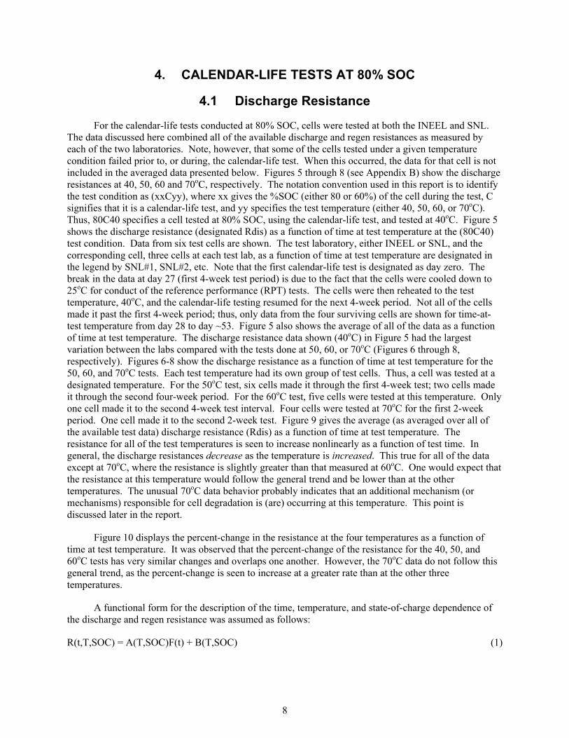
For the calendar-life tests conducted at 80% SOC, cells were tested at both the INEEL and SNL. The data discussed here combined all of the available discharge and regen resistances as measured by each of the two laboratories. Note, however, that some of the cells tested under a given temperature condition failed prior to, or during, the calendar-life test. When this occurred, the data for that cell is not included in the averaged data presented below. Figures 5 through 8 (see Appendix B) show the discharge resistances at 40, 50, 60 and 70oC, respectively. The notation convention used in this report is to identify the test condition as (xxCyy), where xx gives the %SOC (either 80 or 60%) of the cell during the test, C signifies that it is a calendar-life test, and yy specifies the test temperature (either 40, 50, 60, or 70oC). Thus, 80C40 specifies a cell tested at 80% SOC, using the calendar-life test, and tested at 40oC. Figure 5 shows the discharge resistance (designated Rdis) as a function of time at test temperature at the (80C40) test condition. Data from six test cells are shown. The test laboratory, either INEEL or SNL, and the corresponding cell, three cells at each test lab, as a function of time at test temperature are designated in the legend by SNL#1, SNL#2, etc. Note that the first calendar-life test is designated as day zero. The break in the data at day 27 (first 4-week test period) is due to the fact that the cells were cooled down to 25oC for conduct of the reference performance (RPT) tests. The cells were then reheated to the test temperature, 40oC, and the calendar-life testing resumed for the next 4-week period. Not all of the cells made it past the first 4-week period; thus, only data from the four surviving cells are shown for time-at-test temperature from day 28 to day ~53. Figure 5 also shows the average of all of the data as a function of time at test temperature. The discharge resistance data shown (40oC) in Figure 5 had the largest variation between the labs compared with the tests done at 50, 60, or 70oC (Figures 6 through 8, respectively). Figures 6-8 show the discharge resistance as a function of time at test temperature for the 50, 60, and 70oC tests. Each test temperature had its own group of test cells. Thus, a cell was tested at a designated temperature. For the 50oC test, six cells made it through the first 4-week test; two cells made it through the second four-week period. For the 60oC test, five cells were tested at this temperature. Only one cell made it to the second 4-week test interval. Four cells were tested at 70oC for the first 2-week period. One cell made it to the second 2-week test. Figure 9 gives the average (as averaged over all of the available test data) discharge resistance (Rdis) as a function of time at test temperature. The resistance for all of the test temperatures is seen to increase nonlinearly as a function of test time. In general, the discharge resistances decrease as the temperature is increased. This true for all of the data except at 70oC, where the resistance is slightly greater than that measured at 60oC. One would expect that the resistance at this temperature would follow the general trend and be lower than at the other temperatures. The unusual 70oC data behavior probably indicates that an additional mechanism (or mechanisms) responsible for cell degradation is (are) occurring at this temperature. This point is discussed later in the report.

Figure 10 displays the percent-change in the resistance at the four temperatures as a function of time at test temperature. It was observed that the percent-change of the resistance for the 40, 50, and 60oC tests has very similar changes and overlaps one another. However, the 70oC data do not follow this general trend, as the percent-change is seen to increase at a greater rate than at the other three temperatures.

A functional form for the description of the time, temperature, and state-of-charge dependence of the discharge and regen resistance was assumed as follows:

R(t,T,SOC) = A(T,SOC)F(t) + B(T,SOC) (1)

8

Where t is the time at test temperature (in days), T is the test temperature, and SOC is the state of charge of the battery at the start of the calendar-life test. A(T,SOC) and B(T,SOC) are assumed to be functions of the temperature and the state of charge only. The function F(t) is assumed to be only a function of the time at test temperature. The following results will concern the verification of this relationship and to find the functional forms for A(T,SOC), B(T,SOC), and F(t). Once these functions have been determined, then a physical/chemical basis for the functional forms is attempted using the fits to the discharge and regen resistance as a guide.

In an attempt to understand the nonlinear increase in the resistance as a function of time at test temperature (in days), the resistance data were fit to a number of functional forms, as shown in Figures 11 through 17. The reason for plotting the data as various functions of test time is to try and determine not only the time dependence of the resistance increase, but, if the a functional form for the time dependence can be found, to ascertain a physical/chemical process that will account for the resistance increase with time. This information could then be used to understand the process(es) responsible for the cell degradation and in turn suggest possible changes in the construction of the cells. An additional aspect of the determination of the functional form of the time-dependant degradation would be to predict the calendar (and cycle) life of the cells at various test temperatures. In Figures 11 through 17, the data shown in Figure 9 are shown as open symbols, with the best fit (using the listed functional form given in each figure) being represented by dashed lines. Regression analysis for the best fit to the function was obtained using Microsoft Excel. In some of the figures, the coefficients of the fit are given as well. The goodness-of-fit parameter is given by the value R2, which is often referred to as the correlation coefficient. R2 = 1 would be the best correlation of the data to the fitting function. Figure 11 is a linear fit to the time at test temperature. Figure 12 is a quadratic fit. Figure 13 is an exponential fit. Figure 14 is a logarithmic fit. Figure 15 is a fit to the time raised to the 3/2 power (t3/2). Figure 16 is the time at test temperature raised to a power (tn). Figure 17 is the square root of the test time (t1/2). Higher order polynomial fits to the data would, of course, give better fits to the data, but the physical significance would be very hard to explain in terms of a physical/chemical model of the process(es). The functions that correlated the data the best are the square root of test time, and the logarithm of test time. The time raised to a nonintegral power and the quadratic function of the test time also correlate the data well, but a physical/chemical model to account for such time dependence is not known, as is discussed below.

What are the mechanisms responsible for the resistance and increase in the resistance of a lithium ion battery? Zhang et al.5 have discussed the possible mechanisms. The total resistance of the carbon anode and the metal oxide cathode is the sum of the following resistances: (a) electrolyte solution, (b) surface layer, (c) anode and cathode particle to particle contact, (d) anode and cathode to current collector, and (e) charge transfer. The interfacial impedance at the discharged state is larger when compared with the charged state for both the carbon and metal oxide electrodes. Experimental results using electrochemical impedance spectroscopy (EIS) show that the impedance of lithium ion cells, at least with LiCoO2 electrodes, is dominated by the positive electrode, i.e., the cathode. The total cell impedance was found to increases with a decrease in the SOC. Upon consideration of the multitude of possible mechanisms that can lead to resistance increases as the cell ages, the fact that a thin film, often referred too as the SEI (solid electrolyte interface) layer arising from the decomposition of the electrolyte and salt is a likely candidate. When the electrodes are in the charged state, a large portion of the Ni+4 and Co+4 cations will be present in the cathode. These ions have a strong oxidizing power and can react with the electrolyte and salt at the cathode/electrolyte interface. This reaction can cause decomposition of the electrolyte and salt to form a solid electrolyte interface (SEI) layer on the cathode. After extended cycling, the LiNi1-xCoxO2 electrode will be heavily passivated, resulting in a large resistance at the interface. Due to this increase in resistance, the reaction rate will be lower for both lithium ion insertion (intercalation) and deintercalation. The earliest reference to the SEI layer that the authors are aware of is that by Goodenough et al.6, who state that the polymeric surface layer must be in a dynamic state that depends on cell temperature and state of charge, and the extent of aging of the cell. The resistances

9

directly relate to the thickness of the surface layer. The SEI layer that forms on carbonaceous electrode materials consists of many different materials, including LiF, Li2CO3, LiCO-R, Li2O, lithium alkoxides (Li-O-R, where R is a hydrocarbon), nonconductive polymers, and a number of other possible chemical compounds composed of electrolyte and salt decomposition products. The formation of the SEI layer mainly occurs during the initial formation (charging) cycle of the battery. The implication of the SEI layer on the carbon electrode is that it will cause a voltage drop across the layer. This will in turn modify the structure of the double layer at the carbon electrode/electrolyte interface, which generally increases the charge transfer resistance at this interface. Cycling will also cause capacity loss due to damage and disorder in the metal oxide cathode particles. Cycling induces severe strain, high defect densities, and occasional fracture of the particles.5 Severely strained particles exhibit cation disorder. These processes lead to changes in the thermodynamic properties and contact resistance of the metal oxide particles. The accumulation of strain in the particles may cause partial shedding of the electrode material from its current collector. A portion of the lithium ions in the cathode can also become inactive due to cation disorder. However, the main loss in the cathode, for example LiCoO2, is mainly caused by the change in resistance on the surface of the particles.

White et al.7 have also discussed some of the processes known to result in capacity fade in lithium ion cells. These are lithium deposition on the anode (over-charge condition), electrolyte decomposition, anode and/or cathode active material dissolution, phase changes in the anode and cathode materials, and passive film formation over the electrode and current collector surfaces (SEI layer formation). The negative electrode material is metallic (carbon), and, therefore, its contribution to the overall ohmic resistance should be negligible. Its electrical conductivity would not be expected to change with cycling. The metal oxide positive electrode (i.e., the cathode) if composed of LiyCoO2 is a semiconductor. Therefore, its conductivity would be invariant with cycling when it is measured at a certain voltage, i.e., when the lithium-ion content in the cathode solid matrix is kept at a certain level. Ionic conductivity of the electrolyte also does not contribute significantly to the measured conductivity. This was substantiated by the work of Narayanan et al.,8 who state that the process of lithium ion diffusion in the anode and cathode lattice is considerably slower that that in the electrolyte. Therefore, the lithium ion diffusion in the electrode materials would be one of the rate-limiting steps. Thus, the processes affecting the impedance directly relate to the electrode materials and their interactions with the electrolyte, i.e., the SEI layer. Ozawa,9 and Megahed and Scrosati10 have also discussed and confirmed these processes. G. Nagasubramanian,11 using electrochemical impedance spectroscopic (EIS) methods finds that the impedance is mostly due to the cathode. He also found that the interfacial impedance increases as the SOC of the cell decreases. From his measurements, he finds that the cell impedance comes mostly from the cathode/electrolyte interface, not from the anode/electrolyte interface. Guyomard et al.12 also conclude that oxidation of the electrolyte is the main failure mechanism for lithium ion batteries.

The extensive work of Auerbach et al.13, 14 also give an overview of the processes occurring in a lithium ion cell. In parallel to the flux of lithium ions to and into the electrodes, there is a flux of electrons from the current collector to the anode or cathode materials, which balances the charge. This electron flux also has to overcome resistance that exists among the electrode particles, all of which are partially covered by electronically insulating surface films, i.e., an SEI layer. Lithium intercalation into the graphite anode or the metal oxide cathode is a serial multistep process in which lithium ions have to first migrate through the electrolyte and then through the surface films that cover the electrodes. After this migration, insertion into the electrode material is accompanied by a charge transfer at the film/electrode material interface. This is then followed by solid-state diffusion of lithium into the electrode material. Finally, lithium accumulates within crystallographic sites in the bulk electrode material via phase transition(s) between the various intercalation stages. The intercalation stages, particularly for the metal oxide, depend on the crystalline structure of the electrode. The process of charge transfer resistance can be related to three different processes: (1) Li-ion transfer at the solution-surface film interface, (2) Li-ion transfer at the surface film-electrode, and (3) interparticle electron

10

transfer between the particles constituting the electrode material. They also state that the increased resistance observed upon cycling the battery mostly reflects changes in the surface structure of the electrodes. After prolonged cycling, there are phenomena such as expansion and contraction of the electrode material’s volume, which leads to local breakdown of the electrode’s passivation layer (on a microscopic level). This allows continuous reduction and oxidation of the electrolyte species. While the process occurs on a very small scale, it thickens the surface films and consequently the electrode’s impedance increases, particularly in the time constants that relate to lithium ion migration through the surface films, whose increasing thickness upon cycling makes them more resistive. The electrolyte composition has a great impact on the surface films and, depending on its composition, the surface films may be the dominant factor that determines the impedance of the electrode. However, this behavior may not be stable, i.e., the electrode’s impedance, especially in the features that relate to the surface films, increases upon storage and may also change as a result of thermal cycling, and the charging and discharging of the battery.

The above discussion on the processes occurring in a lithium ion battery is only a brief overview of the processes involved. The literature concerning this topic is very extensive. In summary, the overall insertion process of lithium into the battery electrodes is quite complicated. It includes diffusion of lithium ions in the solution phase, their migration through the surface films (SEI layer) covering the electrode particles (which are ionically conducting and electrically insulating), solid state diffusion, accumulation/consumption of lithium in the bulk (accompanied by a flux of electrons that counterbalance the charge), and finally phase transition(s) among the crystalline structures of the electrode materials. Thus, a lithium ion battery is a very dynamic system that depends on its construction, the materials used in its assembly, the rate of charge and discharge, the state of charge, and its temperature. One physical/chemical process that stands out as a candidate for having the greatest impact on the impedance of the cell is the SEI layer, its growth, composition, structure, and thickness.

Looking at possible analogous processes that grow thin films upon a solid surface, one can consider the oxidation of metals. Upon examination of the various reaction rates and corresponding rate equations for the oxidation of metals, it is found that they are functions of a number of factors, such as temperature, oxygen pressure, elapsed time of reaction, surface preparation, and pretreatment of the metal. Although rate equations alone are insufficient for interpretations of oxidation mechanisms, these equations may be used to classify the oxidation of metals and may as such often limit the interpretation to a class of alternative mechanisms. The rate equations most commonly encountered may be classified as logarithmic, parabolic, and linear. They represent only limiting and ideal cases. Deviations from these rate equations and intermediate rate equations are also often encountered. In many instances, it may be difficult to fit rate data to any simple rate equation or combination of rate equations. In the following discussion, an analogy is made between a process occurring at the various surfaces present in a lithium ion battery, the exact nature having been, as yet, not definitively determined, and the growth of an oxide film on a metal surface.15-18

Logarithmic Rate Process. This process is characteristic of the oxidation of a large number of metals at low temperatures where the reaction is initially quite rapid and then drops off to low or negligibly small values. This law is generally found to be applicable for the formation of very thin films of oxide that are between 20 and 40 Angstroms thick and at low temperatures. This behavior is often described by logarithmic rate equations that include the following direct logarithmic rate equation:

Differential form: dx/dt = k/(t + to) (2)

Or

Integral form: x = (k)[Ln(t + to)] + a (3)

11

Where k is the rate constant, to the initial time at which the thickness, x, of the film at time zero from the start of the continued film growth is a. Interpretations of the logarithmic rate law have been based on the adsorption of reactive species, among other processes. Adsorption has been assumed to be the rate determining process during early oxide formation. The processes of adsorption and subsequent nucleation have been shown to lead to the initial nucleation of metal oxide at discrete sites on the metal surface. These oxide islands then proceed to grow rapidly over the metal surface until complete coverage is eventually achieved.

Parabolic Rate Equation. At high temperatures, many metals are found to follow a parabolic time dependence:

Differential form: [dx/dt] = k/x (4)

Integral form: x2 = kt + c (5)

Or

x ∝ t1/2 (6)

Thus, the thickness of the thin film is proportional to the square root of the time that the film growth is occurring. As a general rule, parabolic oxidation signifies that a thermal diffusion process is rate determining.15, 16 Thermal diffusion processes generally have a temperature dependence given by an Arrhenius-like process (discussed later) where the diffusion is given by19

D = Do[exp(-E/RT)] (7)

Where D is the diffusion constant in cm2/sec, Do is the diffusion constant at very high temperature, E is the activation energy associated with the diffusion process, R is the gas constant, and T is the Kelvin temperature. Such a process may include a uniform diffusion of one or both of the reactants through a growing scale, or a uniform diffusion of gas into the metal.

Linear Rate Equation. Linear oxidation may be described by

Differential form: [dx/dt] = k (8)

Or

Integral form: x = kt +c (9)

Where k is the linear rate constant, and c is the integration constant, i.e., the thickness of the film at time t=0. In contrast to the parabolic and logarithmic rate equations, for which the rate of reaction decreases with time, the rate of linear oxidation is constant with time and is thus independent of the amount of gas or metal previously consumed in the reaction. This growth law is found to describe metal oxidation reactions whose rate is controlled by a surface reaction step or by diffusion of one of the reactants to the metal surface.

The analogy to the case of the lithium ion battery is that there would be a film growing on the surface of the anode and/or cathode materials over a period of time that would be temperature dependent. The nature of the thin film would also depend on the electrolyte and the composition of the electrodes. The thickness of this thin film could give rise to an increase in the resistance of the cell as the rate of

12

migration into/out of the anode and/or cathode materials would be impeded by the thin film. The thicker the thin film, the lower the mobility of the lithium ions and, thus, the higher the resistance.

Of the various model fits to the resistance data discussed above, the only ones that have possible physical significance are the logarithm of the test time (shown in Figure 14), the square root of the test time (observed to fit the data quite well as shown in Figure 17), and the test time raised to the first and three-halves power (which are not observed to fit the data, as is shown in Figure 11 or Figure 16). The square root of the test time actually correlates the data the best, as is shown in Figure 17.

The square root of test time could also correspond to a one-dimensional diffusion process.20 to 22 The test time raised to the first power could correspond to a two-dimensional diffusion process, and the test time raised to the 3/2-power to a three dimensional diffusion process.20 to 22 The best fit to the time dependence of the resistance is the square root of the time at test temperature, as the R2 values are quite high, as shown in Figure 17. It may well be that as the cell ages the SEI layer grows in thickness, leading to an increase in the resistance, due to a decrease in the migration rate of the lithium ions into/out of the anode and/or the cathode. The stresses experienced by the cathode particles during change and discharge, and during temperature variation, could lead to fracturing of the particles, as mentioned. This would effectively expose new surfaces on which a SEI layer would grow, thus effectively increasing the cathode resistance. This resistance would be observed as an increase of the discharge and charge resistances measured during the calendar-life test. If the increase in the discharge and regen resistance is proportional to the square root of time at test temperature, then the resistances can be expressed by a function having the form

R(t,T,SOC) = A(T,SOC)t1/2 + B(T,SOC) (10)

Where the discharge and regen resistance, R(t,T,SOC), is a function of time, t, test temperature, T, and state of charge, SOC. That there is a dependence on the SOC is verified by comparing the discharge and regen resistance when the calendar-life test is conducted at 80 or 60% SOC (discussed later in this report). The functions A(T,SOC) and B(T,SOC) are assumed to be functions of the test temperature and SOC. To determine the temperature dependence of the functions A and B, one can plot the fitting coefficients determined from the fits shown in Figure 17 as various function of the test temperature. Shown in Figures 18 and 19 are plots of the function A(T) for the discharge resistance as two different functions of test temperature. Figure 18 plots A as a linear function of temperature (in degrees centigrade). It is obvious that at the test temperatures of 40, 50, and 60oC the A function is fairly linear in temperature, with A decreasing as temperature increases. The value of A at 70oC does not fall on this straight line, which indicates that some additional unknown process is occurring at this temperature that is not a continuation of the process(es) occurring at the lower temperatures. The fitting parameters and the R2 values are given in the figure. In Figure 19, the A parameter is plotted as an inverse function of the temperature (in Kelvins) using an exponential fit, i.e., A =a[exp(b/T)]. This type of function occurs in a number of physical/chemical processes, such as chemical kinetics and in diffusion. A functional form or this kind is generally referred too as Arrhenius-like behavior, as it applies to a chemical reaction or to a diffusion-type of process. Arrhenius initially proposed the following equation for the interpretation of the temperature dependence of chemical reactions. The equation is

k = A[exp(-Ea/RT)] (11)

Where k is the rate of the process, A is a preexponential factor having the same units as k, Ea is an activation energy representative of an energy barrier over which the process (chemical reactant, diffusing species, etc.) must overcome in order to proceed, R is the gas constant, and T is the temperature in Kelvin. For positive values of the activation energy, the rate will increase as the temperature increases. The physical process leading to Arrhenius-like behavior is that the rate of the process requires that an energy

13

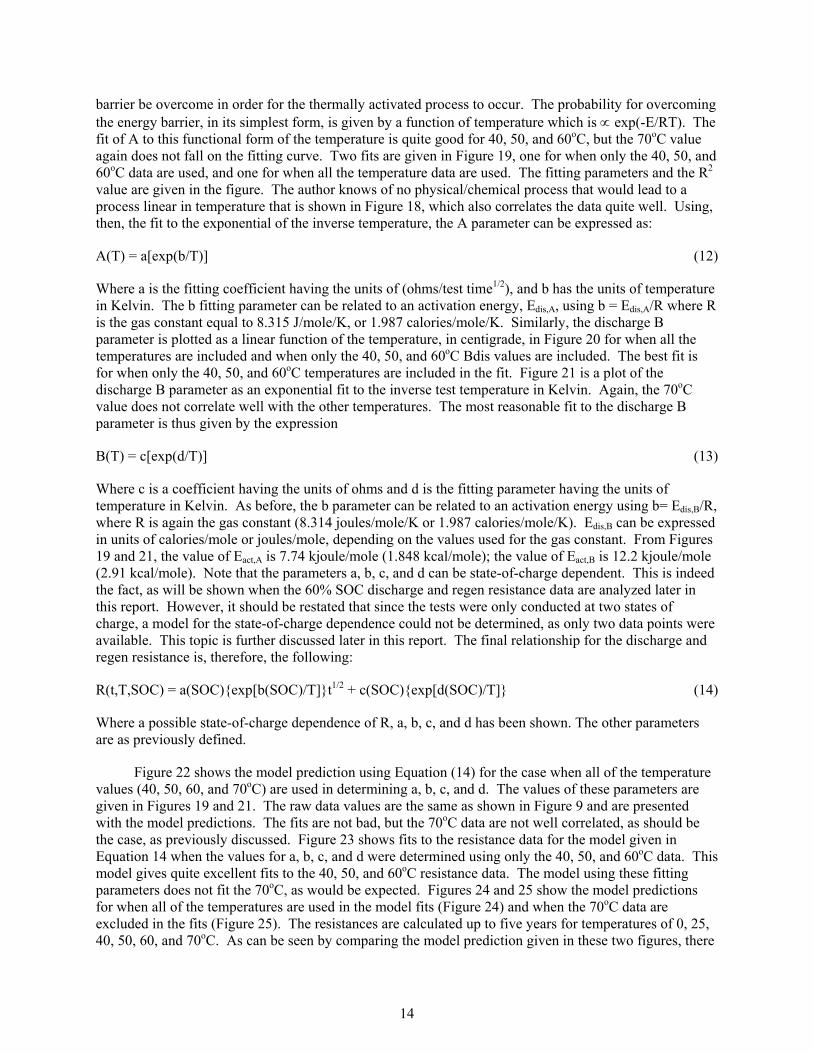
barrier be overcome in order for the thermally activated process to occur. The probability for overcoming the energy barrier, in its simplest form, is given by a function of temperature which is ∝ exp(-E/RT). The fit of A to this functional form of the temperature is quite good for 40, 50, and 60oC, but the 70oC value again does not fall on the fitting curve. Two fits are given in Figure 19, one for when only the 40, 50, and 60oC data are used, and one for when all the temperature data are used. The fitting parameters and the R2 value are given in the figure. The author knows of no physical/chemical process that would lead to a process linear in temperature that is shown in Figure 18, which also correlates the data quite well. Using, then, the fit to the exponential of the inverse temperature, the A parameter can be expressed as:

A(T) = a[exp(b/T)] (12)

Where a is the fitting coefficient having the units of (ohms/test time1/2), and b has the units of temperature in Kelvin. The b fitting parameter can be related to an activation energy, Edis,A, using b = Edis,A/R where R is the gas constant equal to 8.315 J/mole/K, or 1.987 calories/mole/K. Similarly, the discharge B parameter is plotted as a linear function of the temperature, in centigrade, in Figure 20 for when all the temperatures are included and when only the 40, 50, and 60oC Bdis values are included. The best fit is for when only the 40, 50, and 60oC temperatures are included in the fit. Figure 21 is a plot of the discharge B parameter as an exponential fit to the inverse test temperature in Kelvin. Again, the 70oC value does not correlate well with the other temperatures. The most reasonable fit to the discharge B parameter is thus given by the expression

B(T) = c[exp(d/T)] (13)

Where c is a coefficient having the units of ohms and d is the fitting parameter having the units of temperature in Kelvin. As before, the b parameter can be related to an activation energy using b= Edis,B/R, where R is again the gas constant (8.314 joules/mole/K or 1.987 calories/mole/K). Edis,B can be expressed in units of calories/mole or joules/mole, depending on the values used for the gas constant. From Figures 19 and 21, the value of Eact,A is 7.74 kjoule/mole (1.848 kcal/mole); the value of Eact,B is 12.2 kjoule/mole (2.91 kcal/mole). Note that the parameters a, b, c, and d can be state-of-charge dependent. This is indeed the fact, as will be shown when the 60% SOC discharge and regen resistance data are analyzed later in this report. However, it should be restated that since the tests were only conducted at two states of charge, a model for the state-of-charge dependence could not be determined, as only two data points were available. This topic is further discussed later in this report. The final relationship for the discharge and regen resistance is, therefore, the following:

R(t,T,SOC) = a(SOC){exp[b(SOC)/T]}t1/2 + c(SOC){exp[d(SOC)/T]} (14)

Where a possible state-of-charge dependence of R, a, b, c, and d has been shown. The other parameters are as previously defined.

Figure 22 shows the model prediction using Equation (14) for the case when all of the temperature values (40, 50, 60, and 70oC) are used in determining a, b, c, and d. The values of these parameters are given in Figures 19 and 21. The raw data values are the same as shown in Figure 9 and are presented with the model predictions. The fits are not bad, but the 70oC data are not well correlated, as should be the case, as previously discussed. Figure 23 shows fits to the resistance data for the model given in Equation 14 when the values for a, b, c, and d were determined using only the 40, 50, and 60oC data. This model gives quite excellent fits to the 40, 50, and 60oC resistance data. The model using these fitting parameters does not fit the 70oC, as would be expected. Figures 24 and 25 show the model predictions for when all of the temperatures are used in the model fits (Figure 24) and when the 70oC data are excluded in the fits (Figure 25). The resistances are calculated up to five years for temperatures of 0, 25, 40, 50, 60, and 70oC. As can be seen by comparing the model prediction given in these two figures, there

14

are considerable differences in the predictions at longer times at test temperature and also as a function of test temperature. It has been previously acknowledged that the data at 70oC is anomalous due to the onset of different physical/chemical processes at this temperature. This may also be the case at 0oC where the onset of new processes may occur, in particular the decreased ion mobility of the electrolyte.

Upon comparison of the data analysis when the temperature dependence of the resistance is fit using the linear in test temperature relation (see Figures 18 and 20) compared to when the exponential of the inverse temperature is used (see Figures 19 and 21), there arises a difference in the model predictions. The linear temperature model would have the following formula for the resistance as a function of test time at temperature, and test temperature given by

R(t,T) = [eT + f]t1/2 + [gT + h] (15)

The model predictions using this equation are shown in Figure 26. The fit is not bad, excluding the 70oC temperature data. One can also use the logarithm of the test time at temperature to fit the resistance data (see Figure 14). Using the exponential of the inverse of the test temperature, the formula for this correlation is given by the relation

R(t,T) = [i][exp(j/T][Ln(t)] + [k][exp(l/T)] (16)

The model predictions using this form of the model, excluding the 70oC data, to determine i, j, k, and l as before are shown in Figure 27. The fit is not as good, particularly at the shorter times at test temperature.

There arise, of course, differences in the model predictions for longer times at test temperature. These differences are shown in Figure 28. In this figure, the percent difference between the square root of the test time at temperature in combination with the exponential of the inverse temperature, and the approach using the square root of test time at temperature and the linear function of test temperature, are plotted as a function of time at test temperature. The difference between the two approaches is shown over a period of 365 days as a function of the time at test temperature for test temperatures of 25, 40, 50, and 60oC. The model equations used for both approaches are shown in the figure for reference. The data fit for both approaches do not include the fits that include the data at 70oC. This figure shows that there can be considerable differences between the two models (up to ±13%). As there are no data at 25oC or at longer test times, it is currently not possible to verify these predicted differences at these temperatures and test times. Similarly, a comparison can be made with the above three models: square root of test time/exponential of inverse temperature, square-root test time/linear in test temperature, and logarithm of test time/exponential of inverse temperature. The three model predictions for the time at test temperature over a period of 365 days at a test temperature of 25oC are shown in Figure 29 (the model predictions do not include the 70oC data in the fits). As expected, the logarithmic time/exponential inverse temperature model increases rapidly initially and then tends to predict a rather small increase in resistance as time proceeds. There is a small difference in the logarithmic time/exponential inverse temperature model and the square-root time/exponential inverse temperature model at time less than ~25 days, but the difference increases rapidly after that, with the square root time/exponential inverse temperature model predicting a much more rapid resistance increase. The square root time/linear temperature model follows the general shape of the square-root time/exponential inverse temperature model but predicts lower values over the displayed time frame.

There is also another way of explaining the observed exponential of the inverse temperature model. The diffusion constant is often found to vary with temperature, as:19

D = Doexp(-E/RT) (17)

15

Where D is the diffusion constant, or diffusivity, and has the unit of cm2/sec, Do is the limiting diffusion at high temperatures, E is the activation energy for diffusion, R is the gas constant, and T is the temperature in Kelvin. E corresponds to the energy for the thermally activated diffusion of an atom or ion in a solid. The exponential term accounts for the fact that the atom or ion will have sufficient thermal energy to pass over the potential energy barrier a fraction exp(-E/RT) of the time and, thus, is a probability function. The diffusion coefficient of lithium in the electrolyte is four to five orders of magnitude larger than the diffusion coefficient of lithium in the cathode (and anode) and, presumably, through the SEI layer. For the case when the diffusing species are charged, the ionic mobility and the conductivity from the diffusivity are given by the relations19

Ionic mobility ∝ (1/RT)D = (1/RT)Doexp(-E/RT) (18)

Conductivity ∝ Ionic mobility ∝ (1/RT)Doexp(-E/RT) (19)

As the resistivity is inversely proportional to the conductivity, then one may model the resistance, which is proportional to the resistivity, as

Resistance ∝ (RT)exp(E/RT) (20)

This expression is similar to that used previously, except for the additional preexponential temperature term, T, multiplying the exponential function of the inverse of temperature. Equation 20 also predicts that the resistance would decrease with increasing temperature if E is positive. This has been confirmed experimentally. From this relationship, an additional model for the discharge and regen resistance could be fit to the temperature dependence of the resistances using Equation (20). This new model could be compared to the model predictions when there is not the preexponential temperature factor, as in Equation (14). The approach used consists of using the square root of time at test temperature to correlate the time dependence of the discharge and regen resistances as in equation (14). The temperature dependence of A(T) and B(T) would now be A(T) = (a)(T)exp(b/T), and B(T) = (c)(T)exp(d/T), as is described above. In order to fit these expression for A(T) and B(T), the expressions where these parameter were determined from fitting the square root of time dependence, the functions A(T)/T = (a)exp(b/T) and B(T)/T = (c)exp(b/T) were used. These fits are shown in Figures 30 and 31, respectively. For both of the given fits, only the values of A(T)/T and B(T)/T at 40, 50, and 60oC were used, as the 70oC data do not correlate well with the other temperatures. Having determined A(T) and B(T), a fit to Rdis using the experimental data as shown in Figure 9 could be made. Figure 32 shows these results. The fits are quite good, except for the 70oC data. A prediction for the discharge resistance up to five years for temperatures of 0, 25, 40, 50, 60, and 70oC are shown in Figure 33. All the temperature predictions display a nonlinear increase as test time increases. As discussed, as there are no data available at these longer test times, comparison to the predictions using this model cannot be made from this study.

Two models appear to correlate the discharge resistance at temperatures of 40, 50, and 60oC: one model where the temperature is expressed as an exponential of the inverse of the temperature, and one where the temperature is modeled also using an exponential of the inverse temperature but includes a preexponential term in temperature raised to the first power. A comparison is shown in Figure 34 between when the preexponential temperature is used and when it is not. There is only a very slight difference in the two different methods, which is not easily discernable in the figure. Figures 35 and 36 calculate the difference between the two. The greatest difference is for a temperature of 0oC, which amounts to a difference of ~2.5 milliohms over a period of up to one year. These differences are probably within the margin of error of the data used for the curve fitting. The two models have a physical basis in ion diffusion-types of mechanisms for, presumably, the transport of the lithium ions into/out of the electrodes and/or through the SEI layers on each of the electrodes. The ion conductivity model, which has a preexponential temperature factor, is probably the most physically satisfying. However, the data are

16

not sufficiently accurate to discriminate between the conductivity model and when the preexponential temperature is not included in the model, i.e., the pure diffusion model. The conductivity model naturally accounts for the resistance being related to the inverse of the conductivity and the resulting temperature dependence of the resistance decreasing as the temperature increases. This is observed, in general, experimentally. Although the conductivity model has a preexponential factor linear in temperature, the model is dominated by the exponential function of the inverse temperature, at least over the temperature range of the tests.

As an additional correlation of the temperature dependence of the data, Figures 37 through 40 show the analysis of the data when a quadratic function of the temperature is used. This model is not based on any clear physical model, but it is instructive to examine the case when the data are fit using a purely curve fit-based correlation method. Again, a square root of the time at test temperature was used to fit the time dependence of the resistance data. The functions A(T) and B(T) are fit to a function of the form A(T) and B(T) = aT2 + bT + c, where a, b and c are fitting coefficients. The same values of A and B are as previously used as determined from the square root of test time dependence fits. The fits to the values of A(T) and B(T) are shown in Figure 37 and 38, respectively. Observe in the figures that by using the quadratic function the values of A(T) and B(T) at 70oC are included in the fits due to the greater flexibility of the quadratic function. Using these fits as well as the square root of the test time at temperature, the model predictions using the quadratic fit compared to the experimental discharge resistance are shown in Figure 39. By using the quadratic function, the time dependence of the 70oC data is now reasonably accounted for. The model predictions for the other temperatures are also quite good. The model predictions for up to five years are shown in Figure 40. One aspect of this fit with the quadratic function is that at longer test times the discharge resistance at 70oC becomes greater than the resistance at 60oC and 50oC. This is different from the other models discussed. Currently, data are lacking to verify this result. At present there is no physical/chemical basis for using this second-order (or higher polynomial) fitting function other that to simply correlate the test data. This approach does not provide physical/chemical insight into the processes giving rise to the time and temperature dependence of the experimental resistance data.

4.2 Regen Resistance

This section treats the regen resistance for the calendar-life testing at 80% SOC of the ATD Gen 1 cells. The same approach was used as for the treatment of the discharge resistance at 80% SOC. Figures 41 through 44 show all of the regen resistances measured at the INEEL and SNL at the four test temperatures of 40, 50, 60, and 70oC, respectively. The 40, 50, and 60oC regen resistance were measured over a period of initially 4 weeks; the 70oC resistance was measured initially over a period of 2 weeks. As seen in the figures, some of the cells were tested for an additional 4- and 2-week period. The greatest differences in the measured resistances between the two laboratories occurred at 40oC. This difference, ~10 milliohms, was not correlated with any differences in the test methods used at either of the two laboratories. This difference was also seen in the discharge resistance data. At the other test temperatures, the spread in the data was less than ~5 milliohms. The test matrix at each laboratory started with three cells being tested at each test temperature. However, some of the cells designated to be tested at each temperature did not successfully pass the initial RPT at the M-HPPC test condition. The test plan specified that if the cell voltage dropped below the lower voltage limit of 3.0 volts during any one of the states of charge it would be removed from further testing. This accounts for the fact that at some of the temperatures there are data on less than six cells. Figure 45 shows the average of all of the available regen resistance at each of the four test temperatures for the first 4-week period at 40, 50, and 60oC, and for the first 2-week period at 70oC. As was the case for the discharge resistance, the regen resistance increased nonlinearly with increasing time at test temperature. The regen resistance was smaller the higher the test temperature, as was also the case with the discharge resistance. The regen resistance was also lower than the discharge resistance at each of the respective test temperatures. The 70oC resistance,

17

as shown in Figure 45, did not follow the general trend of the other temperatures in that the resistance was the same or higher than the 60oC temperature resistance. This trend for the 70oC regen data is the same as was observed for the 70oC discharge resistance (see Figure 9). Figure 46 plots the percent change in the regen resistance as a function of time at test temperature. The 40, 50, and 60oC values generally group together, while the change in the 70oC resistance was greater. This is similar, but not as dramatic, as that observed in the discharge resistance, as seen in Figure 10. This tends to indicate that something has happened to the cells at this test temperature compared to the lower test temperatures. The detailed nature of the process(es) responsible for this increase in the resistance is, as previously mentioned, not presently known.

The best correlation to the time dependence of the regen resistance was obtained using a square root of the time at test temperature, as was found to be the case for the discharge resistance. The fits to this time dependence, the coefficients, and the goodness-of-fit values are shown in Figure 47. The fits are quite good for all of the test temperatures. Thus, for the regen resistance, the functional form for the time dependence is that given by Equations (1) and (10), which were also used for the discharge resistance. The fitting parameters for each temperature, i.e., the slope being A(T), and the intercept being B(T), were then used to determine the temperature dependence of A and B as before. As was the case for the discharge resistance, the most meaningful temperature dependence for A(T) and B(T) was to use an Arrhenius-like function to determine the temperature dependence of A and B, as given by Equations 12 and 13. Figure 48 shows the plot of the A values as determined in Figure 47 as a function of the inverse temperature in Kelvin, i.e., Arrhenius-like. If the A(T) value for 70oC is excluded, the other three temperature values correlate quite well with an exponential of the inverse temperature. The parameters for the fit are shown in the figure. Similarly, for the B(T) function, the temperatures at 40, 50, and 60oC correlate well with an exponential of the inverse temperature. The 70oC B(T) value does not correlate well with the other three temperatures and was, therefore, excluded from the best-fit expression, as shown in the figure. Using the function as expressed in Equation (10), the model can then be compared to the experiment data, as is done in Figures 50 and 51. Figure 50 shows the comparison of the model when all of the temperatures were used to fit the A(T) and B(T) functions. As seen, the model fits to the data are not good. For comparison, when only the 40, 50, and 60oC A(T) and B(T) parameters are fit to the exponential of the inverse of temperature relation, the fit is greatly improved, as shown in Figure 51. The 70oC data are the exception, as the model predicts considerably smaller values for the resistance. The model predictions for times up to five years are shown in Figures 52 and 53 for when all of the temperatures are used to fit the A(T) and B(T) parameters (Figure 52) and when only the 40, 50, and 60oC temperature data are used (Figure 53). Close comparison of the model predictions reveals a rather large difference in the predicted regen resistances, particularly at the lower temperatures.

As discussed above, the relationship used to correlate the regen temperature data, excluding the 70oC data, is the same used for the discharge resistances. The expression used for the time and temperature correlation is that given by Equations 10, 12, and 13. The use of a model for the temperature dependence based on the ion conductivity model includes a preexponential temperature term, as given by Equation (20). The correlation of this model to the discharge resistance data has been discussed. The results of applying this model for the temperature dependence of the regen resistance are shown in Figure 54 through 57. Figures 54 and 55 show the fits of A(T)/T and B(T)/T to the exponential of the inverse of temperature. In both figures, the 70oC values do not correlate well with the other three temperatures. The fitting coefficients to the other three temperatures are shown in the figures. The model predictions, excluding the 70oC data to fit A(T) and B(T), are shown in Figure 56 compared to the experimental data. Fits to the 40, 50, and 60oC resistances are quite good. As before, the 70oC model predictions do not correlate well with the experimental data. Figure 57 shows the model predictions for up to five years, based on not using the 70oC data to obtain the data fits. Figure 58 shows a comparison of the effect of using the conductivity model (with the preexponential temperature term) with the model predictions when this term is not included. In the figure, the predictions of the two models are shown for up to a period of

18

5 years. As seen, the predictions of the two models are very close for the temperature range shown. This is similar to behavior shown previously in Figures 34 to 36 for the discharge resistance. In summary, using a model based on the physical model of the temperature dependence as relating to the conductivity (i.e., a preexponential term in temperature raised to the first power) compared with not using the preexponential temperature function is not experimentally justified, as present data are insufficient to discriminate between the two models.

To acquire an overall feeling for the differences between the discharge and regen resistances at 80% SOC, Figure 59 shows the data given previously in Figures 9 and 45, except they are plotted on the same graph. General conclusions derived from this figure are that

1. Both the discharge and regen resistances have a nonlinear increase with respect to time at test temperature

2. The discharge resistances are greater than the regen resistances at all of the test temperatures of 40, 50, 60, and 70oC

3. For both the discharge and regen resistances, the higher the test temperature, the lower the resistance, except at 70oC

4. The 70oC data do not follow the general trend of the rest of the data in that the resistance at this temperature is slightly greater than that at 60oC. This observation appears to indicate that new physical/chemical process(es) is (are) occurring that causes the resistance to increase. The exact nature of these process(es) is (are) not presently known.

Table 5 shows the activation energies for both discharge and regen determined using Equation (14) with the square root of test time at temperature time dependence and the exponential of the inverse temperature for the temperature dependence. Given in this table are the activation energies for A(T) and B(T) for when the 70oC data were used in the data fits, and for when only the 40, 50, and 60oC parameters were used. The activation energies are given in both kjoules/mole and kcal/mole. The fits to the 40, 50, and 60oC data are the best ones to consider based on the observations discussed. General trends for the activation energies are that the discharge and regen values are approximately the same order of magnitude for Eact,A and for Eact,B. The activation energies for Eact,B are larger than for Eact,A. The activation energies for Rdis and Rreg are approximately the same within experimental error for both Eact,A and Eact,B. There is presently no explanation for the order of magnitude of these values or why the Eact,B values are greater than the Eact,A values. J. P. Fellner, G. J. Loeber, and S. S. Sandhu23 have discussed measurements on a battery when the cathode was a mixture of LiNiO2 and LiCoO2; the electrolyte was a mixture of PC, EC, and DMC with LiPF6; and the anode was a mixture of two different carbons. They observed that the interfacial resistance for a cell was much higher at lower temperatures, and the interfacial resistance appeared to grow linearly with cycle number. The interfacial resistance had an activation energy for interfacial resistance of 63.5 kjoule/mole. This value for the activation energy was attributed to an activated rate process such as solid-state diffusion and/or electrochemical kinetics. The author has been unable to find literature values for lithium ion diffusion through the SEI layer on the anode or cathode, or its diffusion in the anode or cathode materials for the compositions used in the ATD Gen 1 cells.

19

Table 5. Values of Eact at 80% SOC from analysis of calendar-life test data using the relationship R(t,T) = A(T)t1/2 + B(T), where A(T) = a[exp(Eact,A/RT)], and B(T) = c[exp(Eact,B/RT)]. Eact are activation energies, and a and c are preexponential constants.

Test Conditiona Eact,A Eact,B

Rdis (80C40,50,60,70) 1.58 kjoule/mole(0.378 kcal/mole)

9.04 kjoule/mole(2.16 kcal/mole)

Rdis (80C40,50,60) 7.74 kjoule/mole(1.85 kcal/mole)

12.2 kjoule/mole(2.91 kcal/mole)

Rreg (80C40,50,60,70) 4.36 kjoule/mole(1.04 kcal/mole)

9.20 kjoule/mole(2.20 kcal/mole)

Rreg (80C40,50,60) 8.03 kjoule/mole(1.92 kcal/mole)

12.9 kjoule/mole(3.08 kcal/mole)

a. The terminology (80C40,50,60,70) designates that the calendar-life test was conducted at 80% SOC, and the data analysis used all four test temperatures of 40, 50, 60, and 70oC. Similarly, (80C40,50,60) indicates that the modeling used the data from the 40, 50, and 60oC tests. b. The values for the activation energies were determined from the fits of A(T) and B(T) to an exponential of the inverse of the test temperature in Kelvin. The slope of this fit provides a number, say x, that relates to an activation energy by x = Eact/R, where R is the gas constant (R = 8.314 joules/mole/Kelvin or 1.987 calories/mole/Kelvin).

For completeness, the values of the preexponential constants obtained from the fits for the case of only using the 40, 50, and 60oC data in the fits are shown in Table 6. At present, there is no explanation for these values based on a physical/chemical model nor have literature values been found that provide insight into the values.

Table 6. Values of the preexponential constants a and c at 80% SOC from analysis of calendar-life test data analysis using the relationship R(t,T) = A(T)t1/2 + B(T), where A(T) = a[exp(Eact,A/RT)], and B(T) = c[exp(Eact,B/RT)].

Test Condition(a) a c

Rdis (80C40,50,60) 1.29x10-4 ohm/(day)1/2 4.47 × 10-4 ohm

Rreg (80C40,50,60) 1.03x10-4 ohm/(day)1/2 2.68 × 10-4 ohm a. The terminology (80C40,50,60) indicates that the modeling used the data from the 40, 50, and 60oC tests. b. The values for the preexponential constants a and c were determined from the fits of A(T) and B(T) to an exponential of the inverse of temperature in Kelvin. The intercept of this fit at infinite temperature defines the values of a and c.

20

5. CALENDAR-LIFE TESTS AT 60% SOC

This section discusses the discharge and regen resistance acquired when the cells were at 60% SOC. The test pulse sequence was that shown in Figure 1. The tests were conducted at four temperatures: 40, 50, 60, and 70oC, using the same testing protocols used for the 80% SOC tests discussed previously.

5.1 Discharge Resistance

This section discusses the calendar-life test (see Figure 1 for the discharge/charge test) when the cells were at 60% SOC. All of the test data were acquired at the INEEL. Initially, three cells were tested at each of four temperatures: 40, 50, 60, and 70oC. Figure 60 (see Appendix C) shows all of the discharge resistance test data acquired during testing of the cells. Note that at 60oC only two cells were tested, as one of the cells did not pass the initial RPT. As shown in the figure, a variance was observed among the cells at each of the test temperatures. There is no a priori reason to eliminate one cell or a group of cells from further inclusion in the modeling analysis, as all of the tests were conducted in the same manner. This variance, as well as that observed for the 80% SOC test cells, is most likely due to cell-to-cell variance. Therefore, all of the cell data shown in Figure 60 are included in the following analysis.

Figure 61 shows the average of all of the discharge resistance data at each temperature as a function of time at test temperature. The general trends of the resistances are to increase in nonlinearly as a function of time at test temperature. With increasing temperature, the resistance generally decreases. An exception to this is that the discharge resistances at 50 and 60oC are almost the same, the 60oC temperature data being slightly greater than the resistance at 50oC. This observation is puzzling, and speculation on a possible mechanism that would cause this is difficult. It may well be a result of the state-of-charge influence on the behavior of the cell. This influence may cause new processes to occur at different temperatures, depending on the state of charge of the cell. As noted when discussing the 80% SOC data, it may also be the case that the 70oC resistance data are also unusual due to the same or similar processes responsible for the behavior during testing at this state of charge. Further analysis of the 80% SOC data indicated that some process(es) was occurring at 70oC that caused the resistance to behave in an usual manner. One could also argue that upon closer examination of the data in Figure 60 that cells could be eliminated, which would alter the average discharge resistance data shown in Figure 61. For example, one could eliminate Exp#3 from the 40oC set, as Exp#1 and #2 are quite close to one another. One could also eliminate Exp#3 from the 50oC set, as Exp#1 and #2 are also quite close to one another. The 60oC data set is still problematic, as there are only two cells. If cell Exp#1 is eliminated, the same unusual behavior is observed, as the 60oC resistance does not following the general trend of a decreasing resistance with increasing temperature. If Exp#2 at 60oC is eliminated, the problem is worse. As regards the 70oC cell data, all three of the test cell data are very close to one another, preventing a clear-cut elimination of one or more of the cells from consideration. The following analysis, therefore, includes the average of all of the data in Figure 60. These average resistance values are displayed in Figure 61.

The time dependence of the discharge resistance as fit to the square root of the time at test temperature is shown in Figure 62. Other fitting functions were used in a manner similar to that used for the 80% SOC tests, but the square root of test time at temperature best correlated the data. As was the case for the 80% SOC data, the fit is quite good for all four temperatures. The slope of the fits, A(T), and the intercept at zero time, B(T), are shown in the figure as well as the goodness-of-fit values, R2. The values of A(T) from these fits are plotted as a linear function of the temperature, in degrees centigrade, in Figure 63. The fit is quite reasonable, with none of the A(T) values lying appreciably off the fitting curve. Figure 64 shows the A(T) values plotted as the exponential of the inverse of the Kelvin temperature. Again, the fit is quite good, with none of the values dramatically lying off the fit. In similar

21

fashion, the B(T) values are plotted as a linear function of the temperature, in centigrade, in Figure 65, and as the exponential of the inverse Kelvin temperature, in Figure 65. In both plots, the B(T) values are well correlated with the fit, but the 50 and 60oC values are the furthest from the fit. The temperature dependence of A(T) and B(T) using the exponential of the inverse of the Kelvin temperature in conjunction with the square root of test time at temperature were then used to predict the discharge resistance as a function of test time and temperature. The results are shown in Figure 67, where all of the temperatures were used in determining the variables in the model equation (Equations 10, 12, and 13). The prediction is reasonable for 40 and 70oC, but the model does not fit very well the 50 and 60oC data, as it should not, given that the fits to A(T) and B(T) did not include a higher order polynomial that might have accounted for the reversal of the 5C and 60oC resistance data. Predictions using this model for the discharge resistance for test times up to five years are given in Figure 68. Verification of the prediction over this long of time and for the lower temperatures could not be made from the present data. If the A(T) and B(T) parameters for the test temperature of only 40, 50, and 60oC in conjunction with the exponential of the inverse Kelvin temperature were used, the correlation with the data is shown in Figure 69. The fit to the actual data shown in Figure 69 are not as good as those obtained when all of the temperature data were used in the fits to the temperature dependent A and B parameters. If the data at 60oC are not used for the fits to A(T) and B(T), assuming that an unusual process is occurring at this temperature, the resulting correlation with the data are shown in Figure 70. The longer time predictions up to five years are shown in Figure 71. Examination of the preceding combinations of temperatures used in the fits indicates that inclusion of all test temperatures gives the most reasonable overall fit. It is presently not know why the 70oC temperature for 60% SOC does not influence the resistance to as great an extent as observed to occur for the 80% SOC results. Cell-to-cell variation could possibly account for this discrepancy, as evidenced by the resistance variation at a given test temperature, shown in Figure 60. It may also be that the SOC at which the calendar-life test is conducted has a considerable influence on the temperature at which unusual behavior of the resistance occurs. It would have been very helpful if the tests could have been conducted at additional states of charge to determine the extent of this influence.

5.2 Regen Resistance

The analysis of the regen resistance data at 60% SOC is treated in the same manner as the discharge resistance. The results are presented in this section. Figure 72 shows all of the regen resistance values acquired for all of the cells tested at 60% SOC as a function of time at test temperature. The 40, 50, and 70oC data sets all had data collected from three different cells. There were data from only two cells at 60oC. Variation in the regen resistance was observed among the cells at a given temperature, similar to what was observed for the discharge values. Again, given that there was no compelling reason to eliminate a given cell from the data set, all of the resistance values were used. The averages of all of the resistance data at a given temperature were calculated and are shown in Figure 73. The regen resistance is seen to increase nonlinearly as the test time increased. In general, the higher the test temperature, the lower the resistance. Note that the regen resistances are smaller than the discharge resistances at all temperatures (compare Figures 61 and 73). Using the square root of test time at temperature, the regen resistance at each of the four test temperatures is shown in Figure 74, fitted to this function. The resulting fits are quite good. As before, from the slope and intercept of the fitting curves, the values of A(T) and B(T) were determined, respectively. These values of A(T) and B(T) are plotted as a function of test temperature in degrees centigrade in Figure 75, and as a function of the exponential of the inverse Kelvin temperature in Figures 76. The fitting parameters are shown, as are the goodness-of-fit R2 values. These figures show that the A(T) value at 60oC does not follow the general trend of the other three temperatures, as it lies appreciably off the fitted curve. Also shown in both figures are the results of fitting all the temperatures, and also fitting only the 40, 50, and 70oC temperatures. The fits to B(T) are shown in Figures 77 and 78 using a function linear in the centigrade temperature and as the exponential of the inverse Kelvin temperature, respectively. In these instances, the value of B(T) at 60oC does correlate reasonably well with the fitting curves. Figure 79 shows the results predicted by the model when all the

22

temperatures were used in the fits compared to the experimental data given in Figure 73. The correspondence of the model predictions with the experimental data is not bad at 40 and 70oC, but it is not as well correlated with the 50 and 60oC data. If it is assumed that the 60oC data does not follow the general trend of the other temperatures due to an unusual process occurring at this temperature, then the model predictions are as shown in Figure 80. There is no great improvement in the correlation with the data when compared to when all the test temperatures are used to fit A(T) and B(T) in the model. The model predictions up to five years when all the temperatures are used and when the 60oC data are excluded are shown in Figures 81 and 82, respectively. There are, of course, some differences in the predictions, the greatest being the lower temperature of 0oC. Again, due to lack of data at the longer test times and at the lower temperatures, the model predictions cannot be verified.

As mentioned, the resistance values at some of the test temperatures do not appear to follow a general trend of decreasing as the test temperature increases. For the regen resistances, the 60oC and maybe (as was the case for the 80% SOC tests) the 70oC data, this may be the case. Figure 83 shows the percent change in the regen resistance for all four of the test temperatures. The 40 and 50oC percent change follow one another quite well. The 60oC percent change does not follow the general trend and displays a greater rate of increase with increasing test time than the other temperatures. This anomalous behavior is also reflected in the plots of the A(T) parameter in Figures 75 and 76. The 70oC percent change is slightly lower than at 40 and 50oC. Figure 84 shows the percent change in the discharge resistance for the 60% SOC test condition. The behavior of all of the temperatures is quite similar. Perhaps the 60oC percent change is not following the general trend shown by the other temperatures in that its rate of change is slightly higher. Collectively, these data may substantiate the general observation that at 60 and 70oC for a 60% SOC cell new physical/chemical processes are occurring that are not accounted for in the model. It would certainly be interesting to conduct the tests at other states of charge in combination with temperature effects to assess the influence of SOC on the resistance of the batteries.

It is instructive to compare the average discharge and regen resistances for the (60C40,50,60,70) test on one graph to see the differences between them. This comparison is shown in Figure 85. It is seen that the discharge resistances are higher than the regen resistances at all of the comparable test temperatures. Both sets of resistances increase with increasing test time and generally decrease with increasing temperature. This was the same situation observed for the (80C40,50,60,70) tests, as shown in Figure 59. Further comparison can be made between the discharge resistance for the (80C40,50,60,70) test and the (60C40,50,60,70) test. This comparison is made in Figure 86. At all values of the test temperatures, the discharge resistances for the (80C40,50,60,70) test are greater than the corresponding temperatures for the (60C40,50,60,70), except at 60oC, where the average regen resistance at 60% SOC is higher than it is at 80% SOC. The same is true for the regen resistances, as shown in Figure 87.

If the above model for the increase in resistance as the time at test temperature increases is due to the formation and growth of a thin film by a parabolic growth mechanism on the anode and/or cathode (presumably the SEI layer) is correct, then the square root of test time should correlate the data. This has been verified by the experimental data. One mechanism responsible for the greater discharge and regen resistance for the (80C40,50,60,70) test compared to the (60C40,50,60,70) test is that at the higher state of charge the cathode is more oxidizing due to the greater number of Co+4 and Ni+4 ions in the metal oxide cathode.5 This enhanced oxidizing power of the cathode would lead to the oxidation of the electrolyte, resulting in reduction of the metal ions in the oxide cathode. The oxidized electrolyte and the lithium containing salt (e.g., lithium hexafluorophosphate, LiPF6) would lead to SEI layer compounds, as discussed. The increase in the SEI layer thickness would lead to an increase in the resistance, as the lithium ions would have to migrate through a thicker SEI layer. Based on this conjecture, the resistance at the (80C40,50,60,70) conditions would be greater than at the (60C40,50,60,70) conditions. This model implies a dynamic SEI layer that forms and unforms, depending on the SOC of the cell and/or as cell voltage is being cycled, as it is during the calendar-life cycling test. The cathode material may also be

23

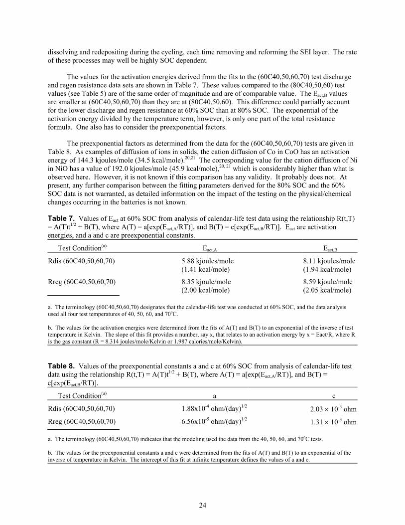
dissolving and redepositing during the cycling, each time removing and reforming the SEI layer. The rate of these processes may well be highly SOC dependent.

The values for the activation energies derived from the fits to the (60C40,50,60,70) test discharge and regen resistance data sets are shown in Table 7. These values compared to the (80C40,50,60) test values (see Table 5) are of the same order of magnitude and are of comparable value. The Eact,B values are smaller at (60C40,50,60,70) than they are at (80C40,50,60). This difference could partially account for the lower discharge and regen resistance at 60% SOC than at 80% SOC. The exponential of the activation energy divided by the temperature term, however, is only one part of the total resistance formula. One also has to consider the preexponential factors.

The preexponential factors as determined from the data for the (60C40,50,60,70) tests are given in Table 8. As examples of diffusion of ions in solids, the cation diffusion of Co in CoO has an activation energy of 144.3 kjoules/mole (34.5 kcal/mole).20,21 The corresponding value for the cation diffusion of Ni in NiO has a value of 192.0 kjoules/mole (45.9 kcal/mole),20, 21 which is considerably higher than what is observed here. However, it is not known if this comparison has any validity. It probably does not. At present, any further comparison between the fitting parameters derived for the 80% SOC and the 60% SOC data is not warranted, as detailed information on the impact of the testing on the physical/chemical changes occurring in the batteries is not known.

Table 7. Values of Eact at 60% SOC from analysis of calendar-life test data using the relationship R(t,T) = A(T)t1/2 + B(T), where A(T) = a[exp(Eact,A/RT)], and B(T) = c[exp(Eact,B/RT)]. Eact are activation energies, and a and c are preexponential constants.

Test Condition(a) Eact,A Eact,B

Rdis (60C40,50,60,70) 5.88 kjoules/mole(1.41 kcal/mole)

8.11 kjoules/mole(1.94 kcal/mole)

Rreg (60C40,50,60,70) 8.35 kjoule/mole (2.00 kcal/mole)

8.59 kjoule/mole(2.05 kcal/mole)

a. The terminology (60C40,50,60,70) designates that the calendar-life test was conducted at 60% SOC, and the data analysis used all four test temperatures of 40, 50, 60, and 70oC. b. The values for the activation energies were determined from the fits of A(T) and B(T) to an exponential of the inverse of test temperature in Kelvin. The slope of this fit provides a number, say x, that relates to an activation energy by x = Eact/R, where R is the gas constant (R = 8.314 joules/mole/Kelvin or 1.987 calories/mole/Kelvin).

Table 8. Values of the preexponential constants a and c at 60% SOC from analysis of calendar-life test data using the relationship R(t,T) = A(T)t1/2 + B(T), where A(T) = a[exp(Eact,A/RT)], and B(T) = c[exp(Eact,B/RT)].

Test Condition(a) a c

Rdis (60C40,50,60,70) 1.88x10-4 ohm/(day)1/2 2.03 × 10-3 ohm

Rreg (60C40,50,60,70) 6.56x10-5 ohm/(day)1/2 1.31 × 10-3 ohm a. The terminology (60C40,50,60,70) indicates that the modeling used the data from the 40, 50, 60, and 70oC tests. b. The values for the preexponential constants a and c were determined from the fits of A(T) and B(T) to an exponential of the inverse of temperature in Kelvin. The intercept of this fit at infinite temperature defines the values of a and c.

24

6. REGROWTH OF RESISTANCE AFTER THE FIRST CALENDAR-LIFE TEST CYCLE

In Figures 5 through 7 for the (80C40,50,60,70) test, it is shown that some of the cells completed the first 4-week calendar-life test at the designated temperature and were then cooled down to 25oC for the RPT test. Upon completion of the RPT test, they were then heated back to the calendar-life test temperature and the next 4-week calendar-life test were conducted. Figure 88 shows the discharge resistance values as a function of the square root of the test time at temperature for three cells at 40, 50, and 60oC that had undergone this test sequence. The vertical dashed line indicates when the cell was cooled down and the RPT test conducted. Before this RPT, the resistance followed the square root of test time quite well, as previously discussed. However, observe that upon reheating the cells to their test temperatures, it takes a period of time for the resistance to increase and begin to follow the extended trend line from the square root of test time relation as determined during the first 4-week calendar-life test. Also observe that this period of time is smaller the higher the test temperature. Using the resistance values at times greater than the time shown by the vertical dashed line and resetting the time to zero, various time-dependent functions were used to account for the time-dependent increase of the resistances during the second 4-week calendar-life test. Figures 89 and 90 (see Appendix D) show the fits to the resistances using a square root of test time at temperature, and the natural logarithm of the test time at temperature, respectively. The fitting parameters and the goodness-of-fit values are shown in the figures. The square root of test time fits the data quite well but does not correlate well with the shorter times. The logarithm of the test time also fits the data very well and better correlates the data at the shorter times. Using the fitting parameters from the logarithmic fit for A(T) and B(T) in Figure 90, these parameters are shown in Figures 91 and 92 as fit to the exponential of the inverse of the Kelvin temperature. The fit of this functional form of the temperature gives excellent correlation to the A(T) and B(T) functions. The final functional form for the regrowth of the discharge resistance using this model is

Rdischarge, regrowth = [a][exp(b/T)][Ln(time at test temperature)] + [c][exp(d/T)] (21)

where a and c are constants, b and d are related to an activation energy, and T is the Kelvin temperature. The value for b was 19.6 kjoule/mole (4.68 kcal/mole). The value for d was 7.42 kjoule/mole (1.77 kcal/mole). At present, there is no rational for the magnitude of these values except to state that they are not outrageously high, i.e., many tens of kjoules, nor are they very low, i.e., less than 1 kjoule/mole. They are also similar in magnitude to the activation energies determined previously for the values of the activation energies for the discharge resistances at 60 and 80% SOC (Tables 5 and 7). The fits of Equation (21) to the experimental data are shown in Figure 93, as well as predictions of what the time dependence of the resistance would be at 25oC. As seen, the correlation to the experimental data is very good over the entire time at test temperature and at the various temperatures. As there were no experiment data at 25oC, the line for 25oC in the figure is only a model prediction. The physical basis of the natural logarithm, as previously discussed, of the time at test temperature as it pertains to the growth of a thin film on a solid is that there has to be an adsorption of a reactant at the surface of the solid at unoccupied reactive sites.15-17 At these sites, the reactant is adsorbed and reacts, thereby nucleating the growth of the film. As the surface sites become occupied, the rate of reaction decreases until complete coverage of the surface is achieved. In the case of the resistance regrowth, following the calendar-life test at an elevated temperature and upon subsequent cooling to 25oC for RPT testing, there may be cracking of the SEI layer due to thermal expansion processes.5, 13 Cracking of the thin film would expose new surface sites upon which a film would grow by the adsorption/reaction/nucleation process. This mechanism as it pertains to lithium ion batteries is at present speculative. It is not known if independent characterization/diagnostic experiments have been conducted to substantiate this model. However, there have been characterization studies, supported by the ATD program, conducted on disassembled ATD cells using a number of surface and bulk sensitive analytical methods. The LBNL group24 have observed nanocrystalline deposits on the surface of test cycled cathode material using atomic force microscopy.

25

These new nanocrystalline deposits formed during test cycling of the cells could result from dissolution/precipitation of the cathode material (or one of its constituents) or by the fracturing of the material during temperature/electrical cycling. An SEI layer could form on the new surfaces of the nanocrystalline deposits, leading to an overall increase in the discharge and regen resistance of the cell as it is cycled.

The same approach and methodology was used to examine the regen resistance regrowth as discussed above for the discharge resistance regrowth. The resistance data are shown in Figure 94 as a function of the time at test temperature for the first calendar-life test/cool down/25oC RPT/second calendar-life test sequence. Fits to the natural logarithm of the time at test temperature for the regrowth regen resistances for temperatures of 40, 50, and 60oC are shown in Figure 95. The fitting parameters are shown as well as the goodness-of-fit parameter. The parameters A(T) and B(T) from these fits are plotted in Figures 96 and 97, respectively, as a function of the exponential of the inverse of the Kelvin temperature. The fits to A(T) and B(T) are quite good. The values for the activation energies from these fits are A(T) equal to 19.5 kjoules/mole (4.67 kcal/mole); for B(T) it is 8.47 kjoules/mole (2.03 kcal/mole). These values are in close agreement with those values determined for the discharge regrowth discussed above. This would imply that the activated process responsible for the regrowth of both the discharge and regen resistances is the same. Using Equation [21] to predict the regen resistance at the temperatures of 40, 50, and 60oC, the results are shown in Figure 98 compared with the experimental data. The fits to the data are very good. Also shown in the figure is the prediction for when the regrowth occurs at 25oC.

If it is assumed that the mechanism for the regrowth of the discharge resistances follows a square root of time dependence, which fits the data fairly well, the derived value for the activation energy for the term that multiplies the square root of time function, A(T), is 19.4 kjoules/mole (4.64 kcal/mole), which is little different from the value resulting from the logarithmic time-dependent mechanism. The value for the activation energy for the B(T) function is 7.40 kjoule/mole (1.77 kcal/mole), which is also essentially the same as the one derived when using the logarithmic time function for the discharge regrowth. The only real justification for using the logarithmic time dependence is that it correlates, the data somewhat better and the mechanism responsible for the resistance regrowth may have its basis in the mechanism for the regrowth of the SEI layer. Note that the activation energy for the A(T) term that multiplies the time-dependent function is larger than that found for the initial growth of the surface layer, the values of which are given in Tables 5 and 7. The observation that the activation energy is higher for the regrowth may be connected with the formation of the initial nucleation sites that may be more difficult to form compared to the growth of a thin film when there is a preexisting film on which new film layers could be deposited. The activation energy of the B(T) function is quite close to those previously found for the activation energy for the initial increase of the resistance during the first calendar-life test period. This may indicate that the process giving rise to the B(T) activation energy does not change during regrowth but is the activation energy required for forming the initial surface film. The physical/chemical process for these observations may be that once the film has formed during the initial elevated temperature calendar-life test, it may provide nucleation sites and/or fresh sites for the subsequent reformation of the SEI layer, and thus an increase in resistance.

The observed result that regrowth of the discharge and regen resistance following a calendar-life test at an elevated temperature, cool down to conduct a room temperature RPT, and subsequent reheat to continue calendar-life testing at elevated temperature follows a logarithmic time dependence indicates a different mechanism for the continued formation of an SEI layer. This logarithmic growth is different from the square root of time dependence observed for the initial growth of the SEI layer. The experimental evidence for a logarithmic growth mechanism is based on the observation that it appears to better correlate with the data. The overall fit to the data is better than the square root of time mechanism, but the latter mechanism fits the data almost as well, and the gross details of the predicted fits to the data do not change appreciably.

26

7. EFFECT OF SOC ON THE CALENDAR-LIFE TESTS

The calendar-life tests were conducted at two states of charge: 60 and 80%. The assumed functional dependence of the discharge and regen resistance, as given in Equations 10 and 14, show that the state of charge at which the cells were tested may influence the discharge and regen resistances. Given that only two different states of charge were studied for the calendar-life test in this study, it is difficult to analyze the effects by using any sort of detailed modeling function. However, it is interesting to examine how the parameters a(SOC), b(SOC), c(SOC), and d(SOC) change and influence resistance, as given by Equation 14:

R(t,T,SOC) = a(SOC){exp[b(SOC)/T]}t1/2 + c(SOC){exp[d(SOC)/T]} (14)

Realize that the following discussion is based on only two states of charge for both the discharge and regen resistances, so only very qualitative interpretations can be given. The values of a(SOC), b(SOC), c(SOC), and d(SOC) that are discussed are taken from Tables 5, 6, 7, and 8. Figure 99 (see Appendix D) shows a(SOC), ohms/(day)1/2, as a function of SOC. It appears that the discharge a(SOC) parameter is greater than the regen a(SOC) at both 60 and 80% SOC. This is verified by the comparison data of Figures 86 and 87 in that the discharge resistances are greater than the regen resistances. However, the discharge a(SOC) appears to be decreasing as the SOC increases, while the regen a(SOC) parameter apparently increases with increasing SOC. This would mean that the discharge resistance would still be greater than the regen resistance at 80% SOC at test times greater than zero, but the difference between the two would not be as great as at 60% SOC. The b(SOC) parameter, in kjoules, which is the activation energy in the exponential of the inverse Kelvin temperature function of A(T,SOC), is shown in Figure 100. The discharge value is seen to increase, while the regen value has only a slight decrease with increasing SOC. In the A(T,SOC) function, which is A(T,SOC) = a(SOC)exp[b(SOC)/RT)], the greater the b(SOC) value, which is positive, the larger A(T,SOC) will be. Also, since b(SOC) is positive, the higher the temperature the smaller the value of A(T,SOC). The larger a(SOC) is, the larger A(T,SOC) will be. It is the product of the a(SOC) function, and the exponential of b(SOC) divided by the Kelvin temperature that yields the value of A(T,SOC). This means that both the a and b parameters must be considered in evaluating their combined influence on A(T,SOC). Note that it is the A(T,SOC) function that appears in the time rate of change of the resistance:

dR(t,T,SOC)/dt = A(T,SOC)/(2t1/2) (22)

Equation 22 means that the time rate of change of the resistance is directly proportional to A(T,SOC), which in turn depends on the temperature and SOC through the a(SOC) and b(SOC) functions. Close examination of the resistance data in Figures 86 and 87 shows that the discharge and regen resistances increase at a greater rate at 80% SOC than at 60% SOC.

Figure 101 shows the c(SOC) parameter that is part of the function accounting for the discharge and regen resistances at time zero. The c(SOC) parameter, in ohms, for both the discharge and regen resistance decreases with increasing percent SOC. This is opposite to what is observed in Figures 86 and 87, as the 80% SOC discharge and regen resistances are greater than the 60% SOC resistances. However, the values of the discharge and regen resistances at time equal to zero are given as B(T,SOC) = c(SOC)exp[d(SOC)/RT], so in order for the resistances to be greater at 80% SOC than at 60% SOC, the function d(SOC), an activation energy, should increase with increasing SOC. This is indeed the case, as shown in Figure 102. In this figure d(SOC), in kjoules/mole, is observed to increase with increasing SOC. The combination of c(SOC) and the exponential of d(SOC) will give rise to the resistances at test time equal to zero. When the actual values for c(SOC) and d(SOC) are used to calculate B(T,SOC), it is found that the discharge and regen resistance values are greater at 80% SOC than they are at 60% SOC. The discharge values, at time zero, are also greater that the regen values at both states of charge. These

27

conclusions are verified by the data in Figures 59, 85, 86, and 87. It is also interesting that the d(SOC) activation energy increases as the SOC increases (Tables 5 and 7, and Figure 102). This may imply that the diffusion of the lithium ions is smaller the higher the state of charge, leading to a greater resistance, as would be expressed by Equations 17 through 20. This in turn may imply that it is either more difficult to intercalate the lithium ions into the carbon anode the higher the SOC, or that it is more difficult to deintercalate the lithium ions from the metal oxide as the SOC increases. Which electrode, or a combination of both, may be responsible? Perhaps it is more difficult for the lithium ions to diffuse through the SEI layer as the SOC increases. At this time, it is not known if either, or both, or neither of these mechanisms is the one responsible.

The very general trends shown in Figures 99 through 102 would require more data at additional states of charge to determine if they are linear or nonlinear in their SOC dependence. This would lead to a more definitive understanding of the physical/chemical processes involved.

28

8. LEAKAGE CURRENT, LEAKAGE RESISTANCE, AND DIFFERENTIAL CAPACITANCE OF ATD GEN 1 CELLS

Representative leakage current, leakage resistance, and differential capacitance data are discussed here for the ATD Gen 1 cells. For the leakage current following each of the C/1 charge steps, there was a duration of ~1.5 hr during which the voltage of the cell was held at 4.1 V and the current monitored. The current during this period slowly decreased after the cell had reached 4.1 V. This test time was not sufficient for the cell to reach a true equilibrium value, but was sufficient to describe the general trends, as is presented below. This current can be referred too as the leakage current, i.e., that amount of charge that the cell will still accept due to losses arising from the resistance of the cell as the cell reaches an equilibrium charge capacity. This decaying leakage current for a representative cell that was undergoing an (80C40) test, i.e., 80% SOC, calendar-life test, and a test temperature of 40oC is shown in Figure 103 (see Appendix E). The data were acquired when the cell was held at 25oC. The four plots are for when the cell had undergone four C/1 discharges (Curve 1): after it had undergone 4 C/1 discharges, a characterization test, and an RPT (Curve 2); after it had undergone four C/1 discharges, a characterization test, an RPT, and a calendar-life test at 40oC (Curve 3); and finally after it had undergone four C/1 discharges, a characterization test, an RPT, and two calendar-life tests at 40oC (Curve 4). The cell failed the RPT test following the second calendar-life test. Note that the logarithm of the current is plotted as a function of test time in hours. Time zero was the time at which the cell reached 4.1 V, and the voltage subsequently held at this value. As seen in the figure, the current decay is not linear, nor is it logarithmic. Attempts at fitting these data to a functional form were not attempted. The point of the plot is that as the cell ages through testing, the leakage current as a function of time does not decrease as rapidly as when the cell was newer. This decrease in the rate of decrease is due to, at present unknown, physical/chemical changes in the cell. The leakage current can be related to a leakage resistance via Ohm’s Law, i.e., Rleakage(ohms) = (4.1 V)/Leakage current (A). These data are shown in Figure 104, where it is seen that the resistance of the cell decreases as the cell ages. Initially, for the fresh cell, the leakage resistance slowly approached a value of ~800 ohms. On further testing, this resistance decreased over the same time period until at the final test at the same test time the resistance was ~270 ohms. Given sufficient time, the other leakage resistances may indeed approach the initial value, but extrapolation to longer times indicates that at the final condition the resistance would be ~400 ohm. Thus, due to testing (aging) some properties of the cell have changed, giving rise to a decreased resistance. This would mean that if the battery is to be trickle charged over a period of time, it would require a higher current to maintain constant voltage.

Figure 105 shows the voltage of the cell (the same cell discussed above) over a voltage range of ~3.3 V to 4.1 V as a function of charge added during four different C/1 discharges at various stages in the cell’s life. The same four states of life of the cell (listed in the figure) are those described above for the leakage current tests; each C/1immediately preceded the leakage current test. It can be seen in the figure that when the cell is new its capacity (Curve 1) is greater than when it has been aged by the various RPTs and calendar-life tests. Just before failing, the cell’s capacity had decreased considerably, from ~0.84 A·h to ~0.66 A·h. Notice that in the curves shown in Figure 105 there is a sharp voltage increase at the beginning of the initiation of the charge pulse. This has been attributed to a voltage increase arising from a model that has a series resistor, sometimes referred to as an equivalent series resistor, connected to the battery. This assumes of course that the battery is not a constant voltage source, but that as charge is removed or added its voltage changes. The voltage on the cell prior to initiation of the constant current charge is Vo; the voltage at the instant of the discharge of current I results in a voltage of VB = Vo + IR for the battery using this model. As the cell ages, this equivalent series resistor, R, is observed to increase. Also notice in the curves in Figure 105 the subtle change in the shape of the four curves as a function of voltage and charge added. To accentuate these differences, the derivative of the charge added with

29

respect to the voltage can be obtained numerically. The method used to calculate the numerical derivative is known as a three-point derivative, given by the formula25

df(xi)/dxi = [1/2h][-f(xi-h) + f(xi+h)] (23)

where h is the change in the difference of the x value from one point to the next, assuming that the change is equal. This formula approximates the derivative of f at point xi by taking the slope of the line through points xi+h and xi-h, i.e., those points on either side of point xi. A modification of his formula if h is not a constant is

df(xi)/dxi = [-f(xi-1) + f(xi+1)]/[(xi+1 - xi-1)] (24)

Equation (23) also means that the derivative of the first and last points in a series of data would not have a derivative taken at that point. Recognize that a numerical derivative accentuates any noise in the data, as is seen in the presentation of the data. The derivative of the charge added (normalized by the total charge put into the cell during the charging portion of the test) with respect to the voltage is referred to as one form of the differential capacitance. The concept of differential capacity has been discussed in the literature.26-28 This is due to the fact that the capacity of the cell times the voltage is equal to the charge contained in the cell, thus CV = Q, and, therefore, the differential capacity is dC = (dQ/dV), where C is the capacity, V is the voltage, and Q is the charge. The purpose of calculating the differential capacity is to determine at what voltage (or SOC) the ability of the cell accepts charge changes as the cell ages. Minima (or maxima) in the differential capacity data have been ascribed to ordered compositions of the host lattice. These minima or maxima are thought to arise from specific structural sites in the anode and cathode materials where the lithium can reside during intercalation. For example, first-principle calculations on LixNiO2

29 have shown there are, at low temperatures, ordered structures predicted to be stable when x = 0.75, 0.66, 0.5, 0.33, and 0.25. These values of x would correspond to states of charge of 25, 34, 50, 67, and 75%. Figure 106 shows the differential capacity of the same cell discussed above for the same four states of life of the cell tested using the (80C40) test condition. The increase in noise due to taking the derivative is apparent in the figure, even though a five-point moving average smoothing (a Microsoft Excel function) of the derivative data was taken in an attempt to reduce the noise. It is also apparent in the figure that the IR-jump in the initial voltage of the battery increases as the cell ages, due to the IR-jump at the onset of the constant current discharge. Notice in this figure that various peaks show up in the differential capacity at various cell voltages. There may be other peaks in the derivative, but one would have to have a model, and a reason, to deconvolute the derivative spectra. This could be done numerically, but a peak shape would have to be assumed, and initial estimates of the peak positions, number of peaks, and an assumed peak shape would have to be input to the deconvolution program. The interpretation of the peaks in Figure 106 is that the higher the peak the greater the ability of the cell to accept charge and, therefore, represents an increase in the capacity of the cell, since the derivative is positive. This is because the slopes of the curves in Figure 105 are positive, indicating the cell is accepting more charge. For example, for Test 1 there are apparent peaks at ~3.51, ~3.67, and ~3.98 V. As the cell ages, the peak at ~3.51 V shifts to higher voltage, as does the peak at 3.67 V. The peak at ~3.98 V remains at about the same voltage. As the cell ages, it is also apparent that the area under the derivative, equal to the charge input to the cell during the charging cycle, is that shown in Figure 105. As a possible aid to research groups conducting diagnostics on the cells, differential capacity curves like those shown in Figure 106 may be used as a guide to investigate the changes in the physical/chemical processes where the greatest change in the cell’s capacity is occurring. Thus, studies at the voltage range of ~3.52, ~3.7, and ~3.97 V may be of particular interest. Note in the differential capacity curves that the apparent shifts in the peaks in the curves may occur because the voltage jump at the beginning of the charge (and for the discharge) causes the peaks to shift. An appropriate way to account for these apparent shifts, which may be nonlinear, needs to be found.

30

Another way of examining the differential capacity for the charging data is to plot it versus the percent SOC of the battery. This plot is shown in Figure 107, where the normalized differential capacity is plotted as a function of the percent SOC of the cell. The percent state of charge was calculated using the formula percent SOC = 100(charge added to cell)/(total charge added to cell during the constant current charge). The total capacity (from ~3.3 to 4.1 V) of the cell was determined from the constant current (C/1) charge test. As seen in Figure 107, the greatest change in the differential capacity occurs at ~10% SOC and at ~30 through 45% SOC. Also notice that presentation of the differential capacity data in this manner eliminates the apparent peak shifts observed in the differential capacity as a function of voltage.

Similar treatment can be applied to the constant current discharge experimental data. For the same cell used in Figures 103 through 107, the constant current C/1 discharge curves are shown at various stages of the cell’s testing in Figure 108. In this figure, there are six discharge curves at various stages in the life of the cell. Discharge curves 1, 2, 3, and 4 were acquired at 25oC. There are also two discharge curves labeled 5, acquired at 40oC, and curve 6, acquired at 8oC. Curve 1 is after the first four C/1 tests. Curve 2 is after the 4 C/1s, a characterization test, and after the first RPT test. Curve 3 is after the 4 C/1s, a characterization test, an RPT, and after the first 4-week calendar-life test conducted at 40oC. Curve 4 is after the 4 C/1s, a characterization test, an RPT, after the first 4-week calendar-life test at 40oC, and after the second calendar-life test also conducted at 40oC. Also shown in the figure are two temperature tests where a C/1 was done at 40oC, curve 5, after the 4 C/1s, a characterization test, and after the RPT test. One test was also done at 8oC, curve 6, after the 4 C/1s, a characterization test, and after the RPT test. As was the case for the charging C/1s, there is a change in the shape of the discharge curves. There is also a change in the IR voltage drop as the cell ages. Especially noticeable is the IR-drop for the 8oC test. The total discharge capacity also decreases as the cell ages.

The differential capacities of the data sets shown in Figure 108 are shown in Figure 109 and 110. Note that the negative of the differential capacity is plotted in this instance. Examining the discharge differential capacity, keep in mind that in this instance the higher the curve the worse the cell is performing, since charge is being removed at a more rapid rate. Figure 109 includes the data sets for the discharge curve after the 4 C/1s and a characterization test (Test 1), and the temperature tests for 40oC (Test 5) and 8oC (Test 6), each of which had 4 C/1 tests and a characterization and RPT test. For the initial 25oC test, Curve 1, three peaks are apparent in the differential capacity curves: at ~3.97, ~3.82, and ~3.54 V. The curves for the 25 and 40oC test, Curve 5, are essentially the same, with a slight decrease in capacity for the 40oC test (~0.92 A·h at 25oC; ~0.89 A·h for 40oC). This is also apparent in Figure 108. Note the IR-drop from 4.1 to ~4.03 V at the start of the constant current discharge. The differential capacity for the test done at 8oC, Curve 6, is dramatically different from the other two tests. There is a substantial IR-drop at the onset of the discharge, and there is also a considerable decrease in the capacity at ~3.65 and at ~3.45 V. This dramatic decrease in the capacity of the cell at 8oC (~0.92 A·h to ~0.77 Ah) is probably due to the decreased ion transport through the electrolyte and separator from the anode to the cathode. One aspect of the discharge (and charge) differential capacity curves is the apparent shift in the curves if the IR-drop (or IR-jump) is substantial. For example, the 8oC data shown in Figure 109 should actually be shifted to the right. One possible method for accounting for this apparent shift is to use the simple equation: Vexperinental = Vbattery - IR, or the actual open circuit voltage (Vbattery) on the battery would be Vbattery = Vexperimental + IR, where Vexperimental is the battery voltage under load, and IR is the IR-drop. (For the case of a constant current charge, the IR term would be negative.) The resistance can be calculated by using the initial voltage drop divided by the current change. To calculate the IR-drop, the values of the voltage and the current from the first two data points collected by the battery tester were used. The data were examined using this model. Figure 110 shows the results. As seen, the data sets move to the right, in particular the 8oC data set. From this figure, it would appear that the change in the 8 and 40oC data occur at all three peaks present in the 25oC test. A better method appears to be required to account for the apparent shift in the differential capacity if the IR-jump or IR-drop is large at the

31

beginning of the charge or discharge. It may well be that the voltage correction is nonlinear, due to nonlinear polarization effects in the battery. As used previously, the differential capacity can be plotted as a function of the percent DOD (percent DOD = 1- percent SOC). The data are plotted in this manner in Figure 111. The greatest change in the differential capacity occurs, as before, for the 8oC data (Test 6), which displays a large decrease in the capacity of the cell over a broad region of ~10 to ~60% DOD. There is little difference between Test 1 at 25oC and Test 5 at 40oC.

A similar treatment of the differential capacity for the four tests conducted at 25oC is shown in Figure 112. Note that the voltages listed are not corrected, as discussed above. The differential capacity changes at various voltage values as the cell ages. The main reduction in the discharge capacity of the cell as it ages appears to be over the voltage range of ~3.6 to 4 V. The issue of the IR voltage drop at the start of the constant current discharge is an open issue, as it would appear that whatever process is giving rise to charge storage at the higher voltage peaks, it is being blocked as the cell ages. Figure 113 shows the differential capacity as a function of percent DOD. The change in the differential capacity as the cell ages is most apparent in the ~10 through ~60% DOD range. One may also plot the differential as the percent SOC that simply reverses the abscissa value, which in turn reverses the curves. This is shown in Figure 114.

A similar treatment as that given above for a (80C40) cell was done on a cell tested, using the (80C70) test. The only difference between these tests is that the (80C70) cell was tested at 70oC for a period of 2 weeks for the calendar-life test instead of being tested for 4 weeks at 40oC. Note that the cell did not pass the medium HPPC test following the first 2-week calendar-life test. The (80C70) test would be considered the more severe test, as the higher temperature should influence and alter the physical/chemical properties of the cell at a more rapid rate. The leakage current at various stages of the aging of the cell are shown in Figure 115, where the logarithm of the leakage current following a C/1 charge is plotted as a function of the test time. Data Set 1 was acquired after the cell had 4 C/1 tests performed on it. Data Set 2 is after 4 C/1s, a characterization test, and an RPT. Data Set 3 is after 4 C/1s, a characterization test, an RPT, and a calendar-life test at 70oC. It is seen that as the cell ages, the leakage current does not fall off as rapidly as when the cell is relatively new. Figure 116 shows corresponding leakage resistances. Comparing the leakage resistance of the cell tested under the (80C40) conditions (Figure 104), observe that the leakage resistance is smaller for the (80C70) test as the cell ages. This means that in order to maintain 4.1 V on the cell, more current, i.e., charge, must be provided to compensate for the greater IR-losses. Therefore, the 70oC calendar-life test for 2 weeks is indeed more severe than the 40oC test for 4 weeks and has a greater impact on subsequent cell performance.

Figure 117 presents data for the same cell discussed above for the (80C70) test from constant current charge tests. The voltage as a function of charge added is graphed for three stages in the cell's life. It is again apparent that as the cell ages, the cell’s capacity (from ~3.2 to 4.1 V) falls from ~0.84 to ~6.4 A·h. Close inspection of the curves themselves reveals there are changes in the shapes of the curves. Using again the concept of the differential capacity to magnify these changes, the resulting curves are shown in Figure 118. In Figure 118, the differential capacity, normalized to the capacity of the cell as measured during the C/1 charge, is shown as a function of the uncorrected cell voltage. Major changes are observed to occur as the cell ages, in particular at ~3.5, ~3.68, and somewhat at ~3.98 V. Comparing these data with the data shown in Figure 106 for the (80C40) test, it is seen that the voltages where the major changes occur are about the same. However, the cell tested using the (80C70) displays a greater change, i.e., a reduced capacity for accepting charge. The changes in the IR-jump are also apparent in this figure. The differential capacity during charging as a function of percent SOC shown in Figure 119 indicates that the major decrease in the capacity of the cell occurs at processes occurring at ~5 to ~15 % SOC, and at ~30 to ~60 % SOC.

32

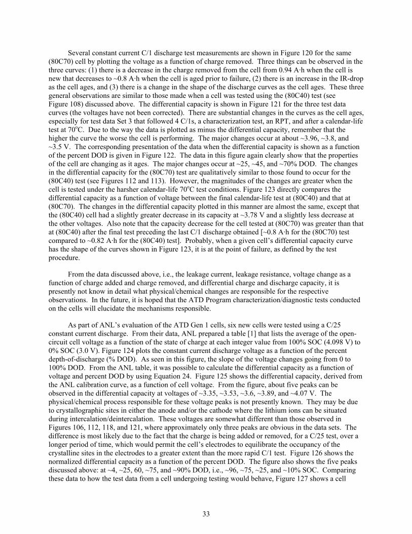
Several constant current C/1 discharge test measurements are shown in Figure 120 for the same (80C70) cell by plotting the voltage as a function of charge removed. Three things can be observed in the three curves: (1) there is a decrease in the charge removed from the cell from 0.94 A·h when the cell is new that decreases to ~0.8 A·h when the cell is aged prior to failure, (2) there is an increase in the IR-drop as the cell ages, and (3) there is a change in the shape of the discharge curves as the cell ages. These three general observations are similar to those made when a cell was tested using the (80C40) test (see Figure 108) discussed above. The differential capacity is shown in Figure 121 for the three test data curves (the voltages have not been corrected). There are substantial changes in the curves as the cell ages, especially for test data Set 3 that followed 4 C/1s, a characterization test, an RPT, and after a calendar-life test at 70oC. Due to the way the data is plotted as minus the differential capacity, remember that the higher the curve the worse the cell is performing. The major changes occur at about ~3.96, ~3.8, and ~3.5 V. The corresponding presentation of the data when the differential capacity is shown as a function of the percent DOD is given in Figure 122. The data in this figure again clearly show that the properties of the cell are changing as it ages. The major changes occur at ~25, ~45, and ~70% DOD. The changes in the differential capacity for the (80C70) test are qualitatively similar to those found to occur for the (80C40) test (see Figures 112 and 113). However, the magnitudes of the changes are greater when the cell is tested under the harsher calendar-life 70oC test conditions. Figure 123 directly compares the differential capacity as a function of voltage between the final calendar-life test at (80C40) and that at (80C70). The changes in the differential capacity plotted in this manner are almost the same, except that the (80C40) cell had a slightly greater decrease in its capacity at ~3.78 V and a slightly less decrease at the other voltages. Also note that the capacity decrease for the cell tested at (80C70) was greater than that at (80C40) after the final test preceding the last C/1 discharge obtained [~0.8 A·h for the (80C70) test compared to ~0.82 A·h for the (80C40) test]. Probably, when a given cell’s differential capacity curve has the shape of the curves shown in Figure 123, it is at the point of failure, as defined by the test procedure.

From the data discussed above, i.e., the leakage current, leakage resistance, voltage change as a function of charge added and charge removed, and differential charge and discharge capacity, it is presently not know in detail what physical/chemical changes are responsible for the respective observations. In the future, it is hoped that the ATD Program characterization/diagnostic tests conducted on the cells will elucidate the mechanisms responsible.

As part of ANL’s evaluation of the ATD Gen 1 cells, six new cells were tested using a C/25 constant current discharge. From their data, ANL prepared a table [1] that lists the average of the open-circuit cell voltage as a function of the state of charge at each integer value from 100% SOC (4.098 V) to 0% SOC (3.0 V). Figure 124 plots the constant current discharge voltage as a function of the percent depth-of-discharge (% DOD). As seen in this figure, the slope of the voltage changes going from 0 to 100% DOD. From the ANL table, it was possible to calculate the differential capacity as a function of voltage and percent DOD by using Equation 24. Figure 125 shows the differential capacity, derived from the ANL calibration curve, as a function of cell voltage. From the figure, about five peaks can be observed in the differential capacity at voltages of ~3.35, ~3.53, ~3.6, ~3.89, and ~4.07 V. The physical/chemical process responsible for these voltage peaks is not presently known. They may be due to crystallographic sites in either the anode and/or the cathode where the lithium ions can be situated during intercalation/deintercalation. These voltages are somewhat different than those observed in Figures 106, 112, 118, and 121, where approximately only three peaks are obvious in the data sets. The difference is most likely due to the fact that the charge is being added or removed, for a C/25 test, over a longer period of time, which would permit the cell’s electrodes to equilibrate the occupancy of the crystalline sites in the electrodes to a greater extent than the more rapid C/1 test. Figure 126 shows the normalized differential capacity as a function of the percent DOD. The figure also shows the five peaks discussed above: at ~4, ~25, 60, ~75, and ~90% DOD, i.e., ~96, ~75, ~25, and ~10% SOC. Comparing these data to how the test data from a cell undergoing testing would behave, Figure 127 shows a cell

33

tested with a (60960) test sequence. This C/25 constant current discharge test was conducted at 60% SOC, and a delta 9% SOC swing (see Table 4 and Figure 4 for the delta 9% cycle-life test). The cycle-life test temperature was 60oC. The voltage as a function of charge removed for a C/25 test is shown for when this cell was fresh compared to when it had been tested to failure, i.e., aged. As observed in this figure, the capacity of the cell had decreased considerably over the course of testing. The shape of the discharge had also changed considerably with aging. The capacity of the fresh cell (determined from the C/25 test) was 0.855 A·h when fresh, compared to 0.714 A·h when aged to failure as defined by the medium HPPC test. The differential capacity of this cell at the two stages in its life were calculated and are shown in Figures 128 and 129 compared to the differential capacity derived from the ANL calibration curve (see Figures 125 and 126). The fresh cell’s differential capacity, as a function of the cell voltage, was very similar to the ANL calibration curve in that the peaks and their height were almost the same. However, when the cell had been aged to failure, the capacity had decreased substantially, as shown in the figure by the increase in the peak heights at various voltages. Note that the aged-to-failure curve has not been corrected for any shifts in the voltage due to the voltage IR-drop at the start of the constant current C/25 discharge. This IR-drop likely causes a shift in the apparent peaks in the differential capacity curve as a function of voltage, as can be seen that the peaks are shifted to lower voltages. Note that there appears to be an increase in the capacity of the cell at ~3.6 V. This may indicate that the lithium is populating this site to a greater extent when the cell is aged compared to when fresh. The major changes would be, assuming a crude voltage correction, at ~3.9, ~3.6, and ~3.53 V. Another way of comparing the cell as it is aged is to examine the differential capacity as a function of the percent DOD. This method avoids any major voltage corrections (assuming they are linear) in order to get the peaks in the curves to line up. Figure 129 displays the differential capacity of the (60960) cell when it is fresh and when it has been aged to failure compared to the differential capacity derived from the ANL calibration curve. The major changes are at ~5, ~35, ~60, ~77, and at ~85% DOD. From the figure, it appears that the cell’s capacity has increased at ~60% DOD as the differential capacity has increased at this percent DOD. This may be another indication that some of the lithium is populating the site(s) responsible for this peak.

In summary, using the concept of differential capacity determined from the constant current charge and discharge tests may be useful for examining the physical/chemical processes responsible for the decrease in the electrical performance of lithium ion batteries as they undergo various test protocols. This information should be of help to researchers conducting physical/chemical characterization/diagnostic evaluations of the batteries and to those doing first-principle theoretical calculations.

34

9. SUMMARY

This report presented the test results pertaining to a group of prototype lithium ion batteries produced by the Advanced Technology Development (ATD) program. The cells had a nominal capacity of 0.9 A·h at a C/1 discharge rate, and a voltage range of 3 to 4.1 V. The composition of the anode was carbon with binders. The composition of the cathode was LiNi0.8Co0.2O2, also containing binders. Aluminum was used as the cathode current collector. The anode current collector was copper. The electrolyte consisted of a 1 M LiPF6 in ethylene carbonate (EC):diethyl carbonate (DEC) in a 1:1 ratio. Polyethylene was used as the separator. The cells were assembled into a 18650-size container. The cells underwent a number of electrical performance tests to determine their electrochemical performance at 25oC. A special calendar-life test was also conducted at elevated temperatures of 40, 50, 60, and 70oC.

The specific test for which the data are presented and discussed was a special calendar-life test conducted once per day for a specified period, depending on the test temperature. The test, consisting of specified discharge and charge protocols, was specially designed to have minimal impact on the cell, yet establish the performance of the cell over a period of time such that the calendar life of the cell could be determined. Specific discharge and regen current levels at specific durations were used at each once-per-day test cycle. The calendar-life test was conducted at 60 and 80% state of charge (SOC). During the calendar-life test, the discharge resistance was determined from the discharge portion of the test. The regen resistance was determined from the regen portion of the test.

The results of the test indicate that both the discharge and regen resistance increased in a nonlinear manner as a function of the test time. The magnitude of the discharge and regen resistance depended on the temperature and SOC at which the test was conducted. General observations derived from this study are as follows:

1. Both the discharge and regen resistances have a nonlinear increase with respect to time at test temperature.

2. The discharge resistance is greater than the regen resistance at all test temperatures of 40, 50, 60, and 70oC.

3. For both the discharge and regen resistances, generally the higher the test temperature, the lower the resistance.

4. The 70oC discharge and regen resistance data at 80% SOC do not follow the general trend of the rest of the data in that the resistance at this temperature is slightly greater than at 60oC. At 60% SOC, the discharge and regen resistance data indicate a process is occurring that causes the 60oC resistance to be greater that at 50oC. At this SOC, the 70oC may also have been influenced. The observation appears to indicate that a new physical/chemical process is occurring that causes the resistance anomalously to increase. They also indicate that the state of charge at which the test was conducted may influence the temperature at which the onset of these new processes occurs. The exact nature of these processes is not presently known.

5. Both the discharge and regen resistances at a given temperature are greater at 80% SOC than they are at 60% SOC.

6. There are also differences in the rate of increase of the resistances in that the 80% SOC resistance increase faster than at 60% SOC.

35

A model was developed to account for the time, temperature, and SOC of the batteries during the calendar-life test. The functional form of the model is given by

R(t,T,SOC) = A(T,SOC)F(t) + B(T,SOC)

where t is the time at test temperature, T is the test temperature, and SOC is the state of charge of the cell at the start of the test. A(T,SOC) and B(T,SOC) are assumed to be functions of the temperature and state of charge; F is assumed to be only a function of the time at test temperature. Using curve fitting techniques for a number of time-dependent functions, it was found that both the discharge and regen resistances were best correlated by a square root of test time dependence. These results led to the relationship for the discharge and regen resistances having the form

R(t,T,SOC) = A(T,SOC)t1/2 + B(T,SOC) .

The square root of time dependence can be accounted for by either a one-dimensional diffusion-type mechanism, presumably of the lithium ions, or by a parabolic growth mechanism for the growth of a thin-film solid electrolyte interface (SEI) layer on the anode and/or cathode. The diffusion-type mechanism would arise from the lithium ions diffusing into/out of the electrodes, through the electrolyte, through the separator, or through the solid electrolyte interface (SEI) layer present on the surface of the electrode materials. The growth of a thin film could relate to the growth of a SEI layer as a function of test time, test condition, and test temperature. The increased thickness of the SEI film would increase the resistance of the cell due to hindrance of the transport of lithium ions through the thicker SEI layer to subsequently be intercalated/deintercalated into the active electrode material. The best physical/chemical model appears at present to be growth of the SEI layer. The present data, however, do not indicate whether the growth of the SEI layer occurs over time at the anode, the cathode, or both. However, characterization results, in particular electrochemical impedance spectroscopic (EIS) methods, indicate that the resistance of the cathode is the major contributor to the resistance of the cell as it ages. The temperature dependence of the resistance was then investigated using various model fits to the functions A(T) and B(T). The results of this exercise lead to a functional form for the functions having an Arrhenius-like form:

A(T) = a[exp(b/T)] and B(T) = c[exp(d/T)]

where a and c are constants and b and d are related to an activation energy, Eb and Ed, by using the gas constant, R, such that b = Eb/R and d = Ed/R. The values of Eb and Ed were determined and found to be about the right order of magnitude (several to several tens of kjoules/mole) for the activated transport of lithium ions. However, no literature values could be found that substantiate these values. It is not known what specific process or processes the determined activation energy values correspond too. The functional form, therefore, for the discharge and regen resistance, including the state of charge (SOC), dependence is then

R(t,T,SOC) = a(SOC){exp[b(SOC)/T]}t1/2 + c(SOC){exp[d(SOC)/T]} .

The a, b, c, and d parameters are explicitly shown as being functions of the SOC. However, due to the lack of testing at SOC values other than 60 and 80% SOC, the exact form of the SOC dependence could not be determined from the experimental data. The function R(t,T,SOC) could then be used to correlate the discharge and regen data and to predict what the resistance would be at different test times at particular test conditions, and different test temperatures.

As part of the calendar-life testing, the cells underwent the calendar-life once-per-day test for a specified period of time at a specified test temperature. The test time was 4 weeks for test temperatures of 40, 50, and 60oC. A 2-week interval was used for the cells tested at 70oC. The cells were then cooled

36

down to 25oC for conducting reference performance tests. The cells were then re-heated to the specified elevated test temperature and the calendar-life test conducted. During conduct of this second and subsequent cyclic testing, the discharge and regen resistances were observed to slowly reach the resistance they had prior to cool down. After this previous resistance was reached, the resistance continued to increase throughout the duration of the test. The above model, and one that has a logarithmic in test time dependence, were applied to this resistance regrowth and found to account for its time and temperature behavior.

Analysis of the C/1 discharge test results allowed determination of the leakage current, i.e., the current required to maintain a given voltage on the cell. In this case, the cells where held constant at 4.1 V. The leakage current was found to decrease quite rapidly in a nonlinear manner for new cells, but after aging by testing, the magnitude of the leakage current was found to increase. The leakage current can be related to a leakage resistance via Ohm’s Law. The leakage resistance was found to decrease as the cell ages, which means that more current, i.e., charge, has to be put into the cell to maintain a given voltage. This increased charge is due to IR-losses in the battery. The IR-losses increase, due to presently unknown detailed processes, as the cell ages.

Further analysis of the C/1 (and C/25) charge and discharge data using the concept of differential capacity was applied to the test data. This analysis simply takes the derivative of the charge added/removed with respect to the cell voltage or charge added or removed during the test. Peaks in the differential capacity are believed to relate to specific intercalation sites within the anode and/or cathode. As the cell ages with testing, the height of the peaks changed, as did their position with respect to the cell voltage or charge/discharge state. The exact nature of these sites, and how the testing influences them, is not presently known. This concept of the differential capacity is believed to be useful to research groups conducting characterization/diagnostic studies on the fresh as well as aged cells. The usefulness arises in that it provides information regarding the voltage and state of charge at which the properties of the cell are changing the most due to use.

37

10. REFERENCES

1. PNGV Test Plan for ATD 18650 Gen 1 Lithium Ion Cells, Rev. 0, EHV-TP-90, March 23, 1999.

2. USABC Electric Vehicle Battery Test Procedures Manual, Rev. 2, DOE/ID-10479, January 1996.

3. PNGV Battery Test Manual, Rev. 2, DOE/ID-10597, August 1999.

4. FY 1999 Progress Report for the Advanced Technology Development Program, U.S. Department of Energy, Office of Advanced Automotive Technologies, 1000 Independence Avenue S.W., Washington, D.C. 20585-0121, March 2000.

5. D. Zhang et al., Journal of Power Sources 91 (2000) 122–129. See also H. Wang et al., Journal of the Electrochemical Society, 146 (1999) 473.

6. M. G. S. R. Thomas, P. G. Bruce, J. B. Goodenough, Journal of the Electrochemical Society, 132 (1985) 1521.

7. P. Arora, R. E. White, M. Doyle, Journal of the Electrochemical Society, 145 (1998) 3647.

8. S. R. Narayanan et al., Journal of the Electrochemical Society, 140, No. 7 (1993) July.

9. K. Ozawa, Solid State Ionics, 69 (1994) 212.

10. S. Megahed, B. S. Scrosati, Journal of Power Sources, 51 (1994) 79.

11. G. Nagasubramanian, FY 1999 Progress Report for the Advanced Technology Development Program, March 2000, p.42. See also: J. Baker, P. Shah, G. Nagasubramanian, D. Doughty, Proceedings of the Electrochemical Society, Volume 99-25, New Jersey, 2000, p. 664.

12. D. Guyomard, J. M. Tarascon, Journal of Power Sources, 54 (1995) 92-98.

13. D. Aurbach et al., Electrochemica Acta, 45 (1999) 67-86.

14. B. Markovsky, M. D. Mikhail, D. Aurbach, Electrochemica Acta, 16-17 (1998) 2287-2304.

15. N. Birks and G. H. Meier, Introduction to High Temperature Oxidation of Metals, Edward Arnold Ltd., London, 1983.

16. Per Kofstad, High-Temperature Oxidation of Metals, John Wiley & Sons, New York, 1966.

17. K. Hauffe, Oxidation of Metals, Plenum Press, New York, 1965.

18. G. E. Blomgren, Journal of Power Sources, 81-82 (1999) 112.

19. C. Kittel, Introduction to Solid State Physics, 4th edition, John Wiley & Sons, New York, 1971.

20. W. Jost, Diffusion in Solids, Liquids, Gases, 3rd printing, Addendum, Academic Press Inc., New York, 1960.

21. J. Crank, The Mathematics of Diffusion, 2nd edition, Clarendon Press, Oxford, 1975.

38

22. Per Kofstad, “Nonstoichiometry, Diffusion, and Electrical Conductivity,” in Binary Metal Oxides, John Wiley & Sons, New York, 1972.

23. J. P. Fellner, G. J. Loeber, S. S. Sandhu, Journal of Power Sources, 81-82 (1999) 867-871.

24. R. Kostecki, et al., “Failure Modes in High-Power Lithium-Ion Batteries for Use in Hybrid Electric Vehicles,” Abstract 190, The 198th Meeting of the Electrochemical Society, October 22-27, 2000, Phoenix, Arizona.

25. R. L. Burden, J. D. Faires, and A. C. Reynolds, Numerical Analysis, Prindle, Weber & Schmidt, Boston, 1978, p. 177.

26. M. D. Levi, D. Aurbach, Electrochimica Acta, 45 (1999) 167-185.

27. J. N. Reimers, J. R. Dahn, Journal of the Electrochemical Society, 139 (1992) 2091.

28. R. R. Haering and R. MacKinnon, “Chapter 4,” in Modern Aspects of Electrochemistry, Vol. 15, eds. B. E. Conway, J. O’M. Bockris, and R. White, Plenum Publishing Co., New York (1981).

29. M. E. Arroyo y de Dompablo et al., “First Principles Investigations in LixNiO2,” Abstract 179, The 198th Meeting of the Electrochemical Society, October 22-27, 2000, Phoenix, Arizona.

39

40

Appendix A

Figures for Calendar-life and Cycle-life Discharge and Regen Resistance Tests on ATD GEN 1 Li-ION Batteries: Experimental Electrical Performance Test Cycles

-4-3.5

-3-2.5

-2-1.5

-1-0.5

00.5

11.5

22.5

33.5

4

0 10 20 30 40 50 60 70 80 90 100 110 12Test time (s)

Test

cur

rent

0

Figure 1. Calendar-life test sequence.

-8-7-6-5-4-3-2-1012345678

0 10 20 30 40 50 60 70Test time (s)

Test

cur

rent

Taper current

80

Figure 2. Delta 3% cycle-life test sequence.

A-1

-8-7-6-5-4-3-2-1012345678

0 10 20 30 40 50 60 70 80 90 100 110 120 130 140 150 160Test time (s)

Test

cur

rent

Taper current

Figure 3. Delta 6% cycle-life test sequence.

-8-7-6-5-4-3-2-1012345678

0 20 40 60 80 100 120 140 160 180 200 220 240Test time (s)

Test

cur

rent

Taper current

Figure 4. Delta 9% cycle-life test sequence.

A-2

Appendix B

Figures for Calendar-life Discharge and Regen Resistance Tests on ATD GEN 1 Li-ION Batteries:

80% State-of-Charge

0.03

0.035

0.04

0.045

0.05

0.055

0.06

0.065

0.07

0.075

0.08

0.085

0 5 10 15 20 25 30 35 40 45 50 55 60Time at test temperature (days)

Rdi

s (o

hms)

SNL#1 SNL#2 SNL#3 INEEL#1 INEEL#2 INEEL#3 Average

40oC

Figure 5. All INEEL and SNL data from calendar-life discharge resistance tests for ATD Gen 1 [80C40] cells.

0.03

0.035

0.04

0.045

0.05

0.055

0.06

0.065

0.07

0.075

0.08

0.085

0 5 10 15 20 25 30 35 40 45 50 55 60Time at test temperature (days)

Rdi

s (o

hms)

SNL#1 SNL#2 SNL#3 INEEL#1 INEEL#2 INEEL#3

50oC

Figure 6. All INEEL and SNL data from calendar-life discharge resistance tests for ATD Gen I [80C50] cells.

B-1

0.03

0.035

0.04

0.045

0.05

0.055

0.06

0.065

0.07

0.075

0.08

0.085

0 5 10 15 20 25 30 35 40 45 50 55 60Time at test temperature (days)

Rdi

s (o

hms)

SNL#1 SNL#2 SNL#3 INEEL#1 INEEL#2

60oC

Figure 7. All INEEL and SNL data from calendar-life discharge resistance tests for ATD Gen I [80C60] cells.

0.03

0.035

0.04

0.045

0.05

0.055

0.06

0.065

0.07

0.075

0.08

0.085

0 5 10 15 20 25 30 35 40 45 50 55 60Time at test temperature (days)

Rdi

s (o

hms)

SNL#1 SNL#2 SNL#3 INEEL#1

70oC

Figure 8. All INEEL and SNL data from calendar-life discharge resistance tests for ATD Gen I [80C70] cells.

B-2

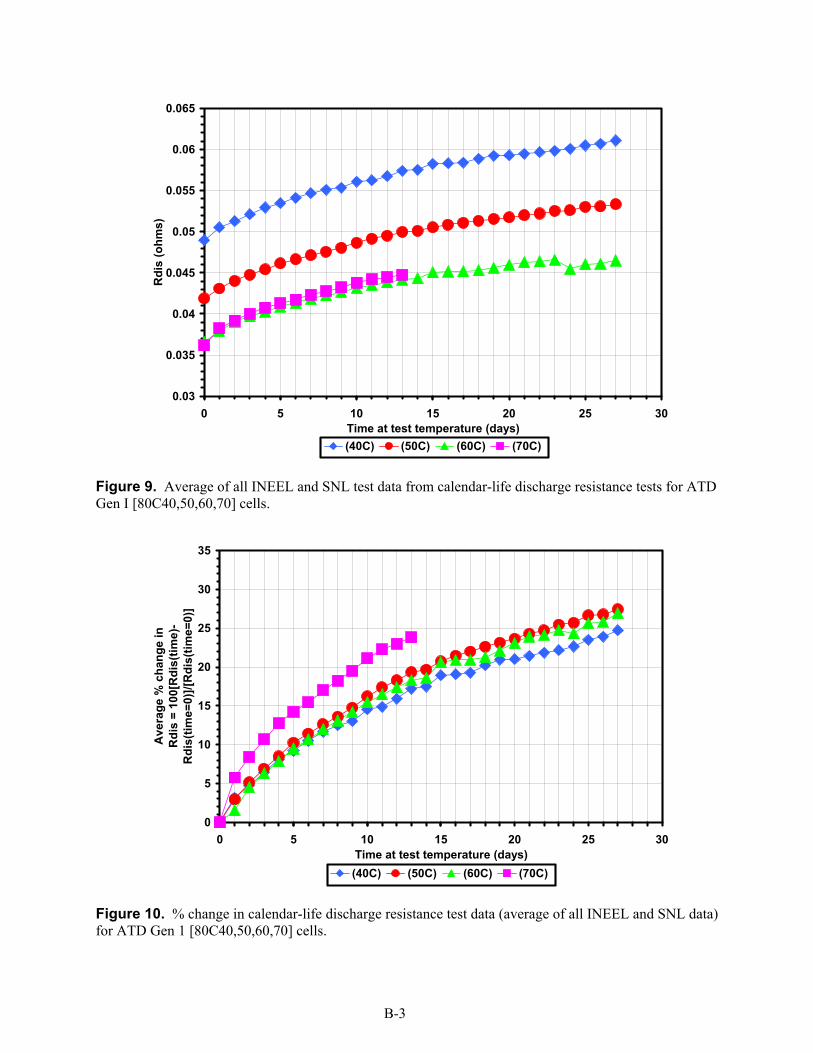
0.03

0.035

0.04

0.045

0.05

0.055

0.06

0.065

0 5 10 15 20 25 30Time at test temperature (days)

Rdi

s (o

hms)

(40C) (50C) (60C) (70C)

Figure 9. Average of all INEEL and SNL test data from calendar-life discharge resistance tests for ATD Gen I [80C40,50,60,70] cells.

0

5

10

15

20

25

30

35

0 5 10 15 20 25 30Time at test temperature (days)

Ave

rage

% c

hang

e in

Rdi

s =

100[

Rdi

s(tim

e)-

Rdi

s(tim

e=0)

]/[R

dis(

time=

0)]

(40C) (50C) (60C) (70C)

Figure 10. % change in calendar-life discharge resistance test data (average of all INEEL and SNL data) for ATD Gen 1 [80C40,50,60,70] cells.

B-3

40oC

50oC

60oC

70oC

0.03

0.035

0.04

0.045

0.05

0.055

0.06

0.065

0 5 10 15 20 25 30Time at test temperature (days)

Rdi

s (o

hms)

(40C) (50C) (60C) (70C)

Fits to Rdis = A*t + B

Figure 11. Average of all INEEL and SNL data from calendar-life discharge resistance tests for ATD Gen I [80C40,50,60,70] cells.

40oC

0.03

0.035

0.04

0.045

0.05

0.055

0.06

0.065

0 5 10 15 20 25 30Time at test temperature (days)

Rdi

s (o

hms)

(40C) (50C) (60C) (70C)

Fits to Rdis = A*t2 + B*t + C

50oC

70oC

60oC

Figure 12. Average of all INEEL and SNL data from calendar-life discharge resistance tests for ATD Gen I [80C40,50,60,70] cells.

B-4

0.03

0.035

0.04

0.045

0.05

0.055

0.06

0.065

0 5 10 15 20 25 30Time at test temperature (days)

Rdi

s (o

hms)

(40C) (50C) (60C) (70C)

Fits to Rdis = A*exp(B*t)

40oC

50oC

60oC

70oC

Figure 13. Average of all INEEL and SNL data from calendar-life discharge resistance tests for ATD Gen I [80C40,50,60,70] cells.

0.03

0.035

0.04

0.045

0.05

0.055

0.06

0.065

0 5 10 15 20 25 30Time at test temperature (days)

Rdi

s (o

hms)

(40C) (50C) (60C) (70C)

60oC

50oC

40oC

70oC

Fits to Rdis = A*ln(B*t) + C

Figure 14. Average of all INEEL and SNL data from calendar-life discharge resistance tests for ATD Gen I [80C40,50,60,70] cells.

B-5

0.03

0.035

0.04

0.045

0.05

0.055

0.06

0.065

0 10 20 30 40 50 60 70 80 90 100 110 120 130 140 150[Time at test temperature (days)]3/2

Rdi

s (o

hms)

(40C) (50C) (60C) (70C)

Fits to Rdis = A*t3/2 + B

70oC

60oC

50oC

40oC

Figure 15. Average of all INEEL and SNL data from calendar-life discharge resistance tests for ATD Gen I [80C40,50,60,70] cells.

(40oC)Rdis = 0.04892t0.0635

R2 = 0.964

(50oC)Rdis = 0.0416E-02t0.0722

R2 =0. 983(60oC)Rdis = 0.0370E-02t0.0694

R2 = 0.972(70oC)

Rdis = 0.0376t0.0643

R2 = 0.9680.03

0.035

0.04

0.045

0.05

0.055

0.06

0.065

0 5 10 15 20 25 30Time at test temperature (days)

Rdi

s (o

hms)

(40C) (50C) (60C) (70C)

Figure 16. Average of all INEEL and SNL data from calendar-life discharge resistance tests for ATD Gen I [80C40,50,60,70] cells.

B-6

(40oC)Rdis = 0.00247t1/2 + 0.0482

R2 = 0.994

(50oC)Rdis = 0.00241t1/2 + 0.0410

R2 = 0.993

(60oC)Rdis = 0.00206t1/2 + 0.0364

R2 = 0.977

(70oC)Rdis = 0.00246t1/2 + 0.0359

R2 =0.9970.03

0.035

0.04

0.045

0.05

0.055

0.06

0.065

0 1 2 3 4 5[Time at test temperature (days)]1/2

Rdi

s (o

hms)

(40C) (50C) (60C) (70C)

6

Figure 17. Average of all INEEL and SNL data from calendar-life discharge resistance tests for ATD Gen I [80C40,50,60,70] cells.

Adis = -2.030x10-5T + 3.328x10-3

R2 = 0.853

0.002

0.0021

0.0022

0.0023

0.0024

0.0025

0.0026

35 40 45 50 55 60 65 70 75Test temperature (oC)

Rdi

s A

par

amet

er

Temps 40,50,60,70C Temps 40,50,60C Linear (Temps 40,50,60C)

Figure 18. Average of all INEEL and SNL calendar-life discharge resistance data for ATD Gen 1 [80C40,50,60,70] cells. Fit to equation: R = A*SQRT[test time in days at temperature] + B.

B-7

Adis = (1.292x10 -4)exp(930.5/T)R2 = 0.833

Adis = (1.312x10 -3)exp(190.0/T)R2 = 0.702

0.002

0.0021

0.0022

0.0023

0.0024

0.0025

0.0026

0.0029 0.00295 0.003 0.00305 0.0031 0.00315 0.0032[1/test temperature] (1/K)

Rdi

s A

par

amet

er

Temps 40,50,60,70°C Temps 40,50,60°CExpon. (Temps 40,50,60°C) Expon. (Temps 40,50,60,70°C)

40oC70oC

Figure 19. Average of all INEEL and SNL calendar-life discharge resistance for ATD Gen 1 [80C40,50,60,70] cells. Fit to equation: R = A*SQRT[test time in days at temperature] + B.

Bdis = -4.152x10 -4T + 6.320x10 -2

R2 = 0.884

Bdis = -5.890x10 -4T + 7.131x10 -2

R2 = 0.983

0.03

0.035

0.04

0.045

0.05

35 40 45 50 55 60 65 70 75Test temperature (°C)

Rdi

s B

par

amet

er

Temps 40,50,60,70°C Temps 40,50,60°CLinear (Temps 40,50,60,70°C) Linear (Temps 40,50,60°C)

Figure 20. Average of all INEEL and SNL calendar-life discharge resistance for ATD Gen 1 [80C40,50,60,70] cells. Fit to equation: R = A*SQRT[test time in days at temperature] + B.

B-8

Bdis = (4.470x10-4)exp(1464/T)R2 =0.994

Bdis = (1.452x10-3)exp(1087/T)R2 = 0.915

0.03

0.035

0.04

0.045

0.05

0.0029 0.00295 0.003 0.00305 0.0031 0.00315 0.0032[1/Test temperature] (1/K)

Rdi

s B

par

amet

er

Temps 40,50,60,70°C Temps 40,50,60°CExpon. (Temps 40,50,60°C) Expon. (Temps 40,50,60,70°C)

40oC

70oC

Figure 21. Average of all INEEL and SNL calendar-life discharge resistance for ATD Gen 1 [80C40,50,60,70] cells. Fit to equation: R = A*SQRT[test time in days at temperature] + B.

0.03

0.035

0.04

0.045

0.05

0.055

0.06

0.065

0 5 10 15 20 25 30Time at test temperature (days)

Rdi

s (o

hms)

(40°C) (50°C) (60°C) (70°C)Model (40°C) Model (50°C) Model (60°C) Model (70°C)

40oC 50oC

70oC60oC

Model includes all 40, 50, 60, 70oC data

Figure 22. Model Predictions for calendar-life discharge resistance data for ATD Gen I [80C40,50,60,70] cells. R = [a*EXP(b/T)][SQRT(test time in days at temperature)] + [c*EXP(d/T)].

B-9

0.03

0.035

0.04

0.045

0.05

0.055

0.06

0.065

0 5 10 15 20 25 30Time at test temperature (days)

Rdi

s (o

hms)

(40C) (50C) (60C) (70C)Model (40C) Model (50C) Model (60C) Model (70C)

40oC

50oC

70oC

60oC

Model does not include 70oC data

Figure 23. Model predictions for calendar-life discharge resistance for ATD Gen I [80C40,50,60,70] Cells. R = [a*EXP(b/T)][SQRT(test time in days at temperature)] + [c*EXP(d/T)].

00.020.040.060.080.1

0.120.140.160.180.2

0.220.240.260.28

0 200 400 600 800 1000 1200 1400 1600 1800 2000Time at test temperature (days)

Rdi

s (o

hms)

0oC25oC40oC50oC60oC70oC

Model includes all 40, 50, 60, 70oC data

1 year 2 years 3 years 4 years 5 years

Figure 24. Model predictions for calendar-life discharge resistance tests for ATD Gen 1 [80C40,50,60,70] Cells. R = [a*EXP(b/T)][SQRT(test time in days at temperature)] + [c*EXP(d/T)].

B-10

00.020.040.060.08

0.10.120.140.160.18

0.20.220.240.260.28

0 200 400 600 800 1000 1200 1400 1600 1800 2000Time at test temperature (days)

Rdi

s (o

hms)

0oC

25oC40oC50oC60oC70oC

Model does not include 70oC data

1 year 2 years 3 years 4 years 5 years

Figure 25. Model predictions for calendar life-discharge resistance tests for ATD Gen 1 [80C40,50,60,70] Cells. R = [a*EXP(b/T)][SQRT(test time in days at temperature)] + [c*EXP(d/T)].

0.03

0.035

0.04

0.045

0.05

0.055

0.06

0.065

0 5 10 15 20 25 30Time at test temperature (days)

Rdi

s (o

hms)

(40C) (50C) (60C) (70C)Model (40C) Model (50C) Model (60C) Model (70C)

40oC

50oC

70oC

60oC

Model does not includes 70oC data

Figure 26. Model predictions for calendar-life discharge resistance for ATD Gen I [80C40,50,60,70] cells. R = [aT +b][SQRT(test time in days at temperature)] + [cT +d].

B-11

0.03

0.035

0.04

0.045

0.05

0.055

0.06

0.065

0 5 10 15 20 25 30Time at test temperature (days)

Rdi

s (o

hms)

(40C) (50C) (60C) (70C)Model (40C) Model (50C) Model (60C) Model (70C)

40oC50oC

70oC 60oC

Model includes all 40, 50, 60oC data

Figure 27. Model predictions for calendar-life discharge resistance data for ATD Gen I [80C40,50,60,70] cells. R = [a*EXP(b/T)][Ln(test time in days at temperature)] + [c*EXP(d/T)].

-15

-12

-9

-6

-3

0

3

6

9

12

15

0 100 200 300 400Time at test temperature (days)

% D

iffer

ence

bet

wee

n ex

pone

ntia

l tem

pera

ture

mod

el a

nd li

near

tem

pera

ture

mod

el [e

xpon

entia

lm

odel

- lin

ear m

odel

]

(25°C) (40°C) (50°C) (60°C)

Models do not include fits to 70 oC data

25oC

40oC

50oC

60oC

Figure 28. Model Predictions for CL Discharge Resistance Tests for ATD Gen 1 [80C40,50,60,70] Cells. R = [a*EXP(b/T)][SQRT(test time in days at temperature)] + [c*EXP(d/T)]; T in K. R = [eT + f][SQRT(test time in days at temperature)] + [gT + h]; T in oC.

B-12

0.02

0.04

0.06

0.08

0.1

0.12

0 100 200 300 400Time at test temperature (days)

Rdi

s (o

hms)

Exp model (25°C) Linear model (25°C) Logarithmic model (25°C)

Models do not include 70°C data fits

SQRT(t); Exponential model

SQRT(t); Linear model

Ln(t); Exponential model

Predictions at 25oC temperature

Figure 29. Model predictions for CL discharge resistance tests for ATD Gen 1 [80C40,50,60,70] cells. R = [a*EXP(b/T)][SQRT(test time in days at temperature)] + [c*EXP(d/T)]; T in K. R = [eT + f][SQRT(test time in days at temperature)] + [gT + h]; T in oC. R = [i*EXP(j/T)][Ln(test time in days at temperature)] + [k*EXP(l/T)]; T in K.

Adis/T = 1.472x10 -7EXP(1253/T)R2 = 0.899

0.000006

0.0000065

0.000007

0.0000075

0.000008

0.0000085

0.0029 0.00295 0.003 0.00305 0.0031 0.00315 0.0032[1/Test temperature] (1/K)

Rdi

s A

/T p

aram

eter

Temps 40,50,60,70°C Temps 40,50,60°C Expon. (Temps 40,50,60°C)

40oC70oC

Figure 30. Average of all INEEL and SNL calendar-life discharge resistance for ATD Gen 1 [80C40,50,60,70] cells. Fit to equation: R = A*SQRT[test time in days at temperature] + B.

B-13

Bdis/T = 5.092x10-7EXP(1787/T)R2 = 0.996

0.0001

0.00011

0.00012

0.00013

0.00014

0.00015

0.00016

0.0029 0.00295 0.003 0.00305 0.0031 0.00315 0.0032[1/Test temperature] (1/K)

Rdi

s B

/T p

aram

eter

Temps 40,50,60,70°C Temps 40,50,60°C Expon. (Temps 40,50,60°C)

40oC

70oC

Figure 31. Average of all INEEL and SNL calendar-life discharge resistance for ATD Gen 1 [80C40,50,60,70] cells. Fit to equation: R = A*SQRT[test time in days at temperature] + B.

0.03

0.035

0.04

0.045

0.05

0.055

0.06

0.065

0 5 10 15 20 25 30Time at test temperature (days)

Rdi

s (o

hms)

(40C) (50C) (60C) (70C)Model (40C) Model (50C) Model (60C) Model (60C)

40oC

50oC

70oC

60oC

Model does not include 70oC data

Figure 32. Model predictions for calendar-life discharge resistance for ATD Gen I [80C40,50,60,70] Cells. R = [a*T*EXP(b/T)][SQRT(test time in days at temperature)] +[c*T*EXP(d/T)].

B-14

00.020.040.060.08

0.10.120.140.160.18

0.20.220.240.260.28

0 200 400 600 800 1000 1200 1400 1600 1800 2000Time at test temperature (days)

Rdi

s (o

hms)

0oC

25oC40oC50oC60oC70oC

Model does not include 70oC data

1 year 2 years 3 years 4 years 5 years

Figure 33. Model predictions for calendar-life discharge resistance tests for ATD Gen 1 [80C40,50,60,70] cells. R = [a*T*EXP(b/T][SQRT(test time in days at temperature)] + [c*T*EXP(d/T)].

00.020.040.060.08

0.10.120.140.160.18

0.20.220.240.260.28

0 200 400 600 800 1000 1200 1400 1600 1800 2000Time at test temperature (days)

Rdi

s (o

hms)

0oC25oC40oC50oC60oC70oC

Model does not include 70oC data

1 year 2 years 3 years 4 years 5 years

Figure 34. Model predictions for calendar-life discharge resistance tests for ATD Gen 1 [80C40,50,60,70] cells; comparison between: R = [a*EXP(b/T)][SQRT(test time in days at temperature)] + [c*EXP(d/T)] and R = [e*T*EXP(f/T)][SQRT(test time in days at temperature)] + [g*T*EXP(h/T)].

B-15

-0.0025

-0.002

-0.0015

-0.001

-0.0005

0

0.0005

0 50 100 150 200 250 300 350 400Time at test temperature (days)

Diff

eren

ce b

etw

een

mod

el p

redi

ctio

n fo

r Rdi

s(o

hms)

[(A) -

(B)]

Difference (0°C) Difference (25°C) Difference (40°C)Difference (50°C) Difference (60°C) Difference (70°C)

50oC40oC60oC70oC25oC0oC

Models included all 40, 50, 60 oC data

Figure 35. Model predictions for calendar-life discharge resistance tests for ATD Gen 1 [80C40,50,60,70] cells; cifference between: (A): R = [a*EXP(b/T)][SQRT(test time)] + [c*EXP(d/T)] (B): R = [e*T*EXP(f/T)][SQRT(test time)] + [g*T*EXP(h/T)].

-0.0001-0.00009-0.00008-0.00007-0.00006-0.00005-0.00004-0.00003-0.00002-0.00001

00.000010.000020.000030.000040.00005

0 50 100 150 200 250 300 350 400Time at test temperature (days)

Diff

eren

ce b

etw

een

mod

el p

redi

ctio

n fo

r Rdi

s(o

hms)

[(A) -

(B)]

Difference (40°C) Difference (50°C) Difference (60°C) Difference (70°C)

50oC40oC60oC70oC

Models included all 40, 50, 60 oC data

Figure 36. Model predictions for calendar-life discharge resistance tests for ATD Gen 1 [80C40,50,60,70] cells; difference between: (A): R = [a*EXP(b/T)][SQRT(test time)] + [c*EXP(d/T)] (B): R = [e*T*EXP(f/T)][SQRT(test time)] + [g*T*EXP(h/T)]

B-16

Adis = 1.140x10 -6T2 - 1.291x10 -4T + 5.859x10 -3

R2 = 0.521

0.002

0.0021

0.0022

0.0023

0.0024

0.0025

0.0026

35 40 45 50 55 60 65 70 75Test temperature ( oC)

Rdi

s A

par

amet

er

Temperatures 40,50,60,70°C Poly. (Temperatures 40,50,60,70°C)

Figure 37. Average of all INEEL and SNL calendar-life discharge resistance data for ATD Gen 1 [80C40,50,60,70] cells. Fit to equation: R = A*SQRT[test time in days at temperature] + B.

Bdis = 1.675x10 -5T2 - 2.258x10 -3T + 1.118x10 -1

R2 = 0.999

0.03

0.035

0.04

0.045

0.05

35 40 45 50 55 60 65 70 75Test temperature (C)

Rdi

s B

par

amet

er

Temperatures 40,50,60,70°C Poly. (Temperatures 40,50,60,70°C)

Figure 38. Average of all INEEL and SNL calendar-life discharge resistance for ATD Gen 1 [80C40,50,60,70] cells. Fit to equation: R = A*SQRT[test time in days at temperature] + B.

B-17

0.03

0.035

0.04

0.045

0.05

0.055

0.06

0.065

0 5 10 15 20 25 30Time at test temperature (days)

Rdi

s (o

hms)

(40C) (50C) (60C) (70C)Model (40C) Model (50C) Model (60C) Model (70C)

40oC

50oC

70oC60oC

Model includes all 40, 50, 60, 70oC data

Figure 39. Model predictions for calendar-life discharge resistance data for ATD Gen I [80C40,50,60,70] cells. R = [aT2 + bT + c][SQRT(test time in days at temperature)] + [dT2 + eT + f].

00.020.040.060.080.1

0.120.140.160.180.2

0.220.240.260.280.3

0.320.340.360.38

0 200 400 600 800 1000 1200 1400 1600 1800 2000Time at test temperature (days)

Rdi

s (o

hms)

0oC25oC40oC70oC50oC60oC

Model includes all 40, 50, 60, 70oC data

1 year 2 years 3 years 4 years 5 years

Figure 40. Model predictions for calendar-life discharge resistance tests for ATD Gen 1 [80C40,50,60,70] cells. R = [aT2 + bT + c][SQRT(test time in days at temperature)] + [dT2 + eT + f].

B-18

0.03

0.035

0.04

0.045

0.05

0.055

0.06

0.065

0.07

0.075

0.08

0.085

0 5 10 15 20 25 30 35 40 45 50 55 60Time at test temperature (days)

Rre

g (o

hms)

SNL#1 SNL#2SNL#3 INEEL#1INEEL#2 INEEL#3Average all INEEL and SNL (40C)

40oC

Figure 41. All INEEL and SNL data calendar-life regen resistance for ATD Gen 1 Cells [80C40].

0.025

0.03

0.035

0.04

0.045

0.05

0.055

0.06

0.065

0.07

0.075

0.08

0.085

0 5 10 15 20 25 30 35 40 45 50 55 60Time at test temperature (days)

Rre

g (o

hms)

INEEL#4 (50°C) INEEL#6 (50°C) INEEL#43 (50°C)SNL#P001 (50°C) SNL#P002 (50°C) SNL#P003 (50°C)

50oC

Figure 42. All INEEL and SNL data from calendar-life regen resistance tests for ATD Gen I cells [80C50].

B-19

0.025

0.03

0.035

0.04

0.045

0.05

0.055

0.06

0.065

0.07

0.075

0.08

0.085

0 5 10 15 20 25 30 35 40 45 50 55 60Time at test temperature (days)

Rre

g (o

hms)

INEEL#1 INEEL#2 SNL#1 SNL#2 SNL#3

60oC

Figure 43. All INEEL and SNL data from calendar-life regen resistance tests for ATD Gen I cells [80C60]

0.025

0.03

0.035

0.04

0.045

0.05

0.055

0.06

0.065

0.07

0.075

0.08

0.085

0 5 10 15 20 25 30 35 40 45 50 55 60Time at test temperature (days)

Rre

g (o

hms)

INEEL#1 SNL#1 SNL#2 SNL#3

70oC

Figure 44. All INEEL and SNL data from calendar-life regen resistance tests for ATD Gen I cells [80C70].

B-20

0.025

0.03

0.035

0.04

0.045

0.05

0.055

0 5 10 15 20 25 30Time at test temperature (days)

Rre

g (o

hms)

(40°C) (50°C) (60°C) (70°C)

Figure 45. Average of all INEEL and SNL data from calendar-life regen resistance tests for ATD Gen I cells [80C40,50,60,70].

0

5

10

15

20

25

30

35

0 5 10 15 20 25 30Time at test temperature (days)

Ave

rage

% c

hang

e in

Rre

g =

100[

Rre

g(tim

e)-

Rre

g(tim

e=0)

]/[R

reg(

time=

0)]

(40°C) (50°C) (60°C) (70°C)

Figure 46. Percent change in calendar-life regen resistance test data (Average of all INEEL and SNL data) for ATD Gen 1 cells [80C40,50,60,70].

B-21

(40oC)Rreg = 0.00221t 1/2 + 0.0381

R2 = 0.995

(50oC)Rreg = 0.00212t 1/2 + 0.0320

R2 = 0.994

(60oC)Rreg = 0.00183t 1/2 + 0.0283

R2 = 0.988(70oC)Rreg = 0.00197t 1/2 + 0.0283

R2 = 0.993

0.025

0.03

0.035

0.04

0.045

0.05

0.055

0 1 2 3 4 5[Time at test temperature (days)]1/2

Rre

g (o

hms)

(40°C) (50°C) (60°C) (70°C)

6

Figure 47. Average of all INEEL and SNL data from calendar-life regen resistance tests for ATD Gen I [80C40,50,60,70] cells.

Areg = (1.027x10 -4)exp(966.1/T)R2 = 0.884

0.0017

0.0018

0.0019

0.002

0.0021

0.0022

0.0023

0.0029 0.00295 0.003 0.00305 0.0031 0.00315 0.00321/Test temperature (1/K)

Rreg

A p

aram

eter

Temps 40,50,60,70°C Temps 40,50,60°C Expon. (Temps 40,50,60°C)

40oC

70oC

Figure 48. Average of all INEEL and SNL calendar-life regen resistance for ATD Gen 1 [80C40,50,60,70] cells. Fit to equation: R = A*SQRT[test time in days at temperature] + B.

B-22

Breg = (2.683x10 -4)exp(1550/T)R2 = 0.993

0.025

0.03

0.035

0.04

0.0029 0.00295 0.003 0.00305 0.0031 0.00315 0.0032[1/Test temperature] (1/K)

Rre

g B

par

amet

er

Temps 40,50,60,70°C Temps 40,50,60°C Expon. (Temps 40,50,60°C)

40oC

70oC

Figure 49. Average of all INEEL and SNL calendar-life regen resistance for ATD Gen 1 [80C40,50,60,70] cells. Fit to equation: R = A*SQRT[test time in days at temperature)] + B.

0.025

0.03

0.035

0.04

0.045

0.05

0.055

0 5 10 15 20 25 30Time at test temperature (days)

Rre

g (o

hms)

(40C) (50C) (60C) (70C)Model (40C) Model (50C) Model (60C) Model (70C)

40oC

70oC

50oC

60oC

Model includes all 40, 50, 60, 70oC data

Figure 50. Model predictions for calendar-life regen resistance data for ATD Gen I [80C40,50,60,70] cells. R = [a*EXP(b/T)][SQRT(test time in days at temperature)] + [c*EXP(d/T)].

B-23

0.025

0.03

0.035

0.04

0.045

0.05

0.055

0 5 10 15 20 25 30Time at test temperature (days)

Rre

g (o

hms)

(40C) (50C) (60C) (70C)Model (40C) Model (50C) Model (60C) Model (70C)

40oC

70oC

50oC

60oC

Model does not include 70oC data

Figure 51. Model predictions for calendar-life regen resistance for ATD Gen I [80C40,50,60,70] cells. R = [a*EXP(b/T)][SQRT(test time in days at temperature)] + [c*EXP(d/T)].

0

0.02

0.04

0.06

0.08

0.1

0.12

0.14

0.16

0.18

0.2

0.22

0.24

0 200 400 600 800 1000 1200 1400 1600 1800 2000Time at test temperature (days)

Rre

g (o

hms)

0oC25oC40oC50oC60oC70oC

Model includes all 40, 50, 60, 70oC data

1 year 2 years 3 years 4 years 5 years

Figure 52. Model predictions for calendar-life regen resistance data for ATD Gen I [80C40,50,60,70] cells. R = [a*EXP(b/T)][SQRT(test time in days at temperature)] + [c*EXP(d/T)].

B-24

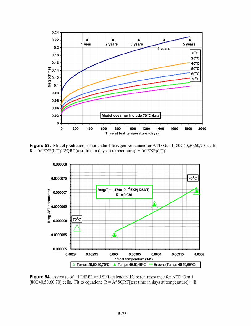
0

0.02

0.04

0.06

0.08

0.1

0.12

0.14

0.16

0.18

0.2

0.22

0.24

0 200 400 600 800 1000 1200 1400 1600 1800 2000Time at test temperature (days)

Rre

g (o

hms)

0oC

25oC40oC50oC60oC70oC

Model does not include 70oC data

1 year 2 years 3 years4 years

5 years

Figure 53. Model predictions of calendar-life regen resistance for ATD Gen I [80C40,50,60,70] cells. R = [a*EXP(b/T)][SQRT(test time in days at temperature)] + [c*EXP(d/T)].

Areg/T = 1.170x10 -7EXP(1289/T)R2 = 0.930

0.000005

0.0000055

0.000006

0.0000065

0.000007

0.0000075

0.000008

0.0029 0.00295 0.003 0.00305 0.0031 0.00315 0.00321/Test temperature (1/K)

Rre

g A

/T p

aram

eter

Temps 40,50,60,70°C Temps 40,50,60°C Expon. (Temps 40,50,60°C)

40oC

70oC

Figure 54. Average of all INEEL and SNL calendar-life regen resistance for ATD Gen 1 [80C40,50,60,70] cells. Fit to equation: R = A*SQRT[test time in days at temperature] + B.

B-25

Breg/T = 3.055x10 -7EXP(1873/T)R2 = 0.996

0.00007

0.00008

0.00009

0.0001

0.00011

0.00012

0.00013

0.0029 0.00295 0.003 0.00305 0.0031 0.00315 0.0032[1/Test temperature] (1/K)

Rre

g B/

T pa

ram

eter

Temps 40,50,60,70°C Temps 40,50,60°C Expon. (Temps 40,50,60°C)

40oC

70oC

Figure 55. Average of all INEEL and SNL calendar-life regen resistance for ATD Gen 1 [80C40,50,60,70] cells. Fit to equation: R = A*SQRT[test time in days at temperature)] + B.

0.025

0.03

0.035

0.04

0.045

0.05

0.055

0 5 10 15 20 25 30Time at test temperature (days)

Rre

g (o

hms)

(40C) (50C) (60C) (70C)Model (40C) Model (50C) Model (60C) Model (70C)

40oC

70oC

50oC

60oC

Model does not include 70oC data

Figure 56. Model predictions for calendar-life regen resistance for ATD Gen I [80C40,50,60,70] cells. R = [a*T*EXP(b/T)][SQRT(test time in days at temperature)] + [c*T*EXP(d/T)].

B-26

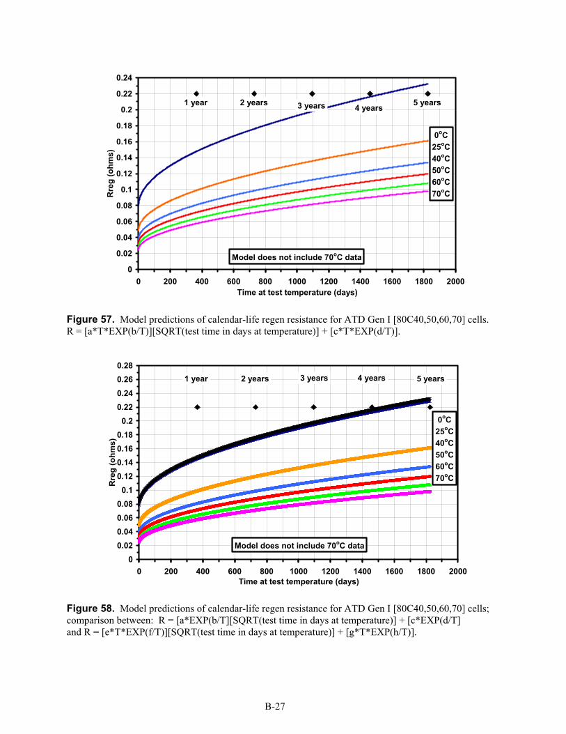
0

0.02

0.04

0.06

0.08

0.1

0.12

0.14

0.16

0.18

0.2

0.22

0.24

0 200 400 600 800 1000 1200 1400 1600 1800 2000Time at test temperature (days)

Rre

g (o

hms)

0oC25oC40oC50oC60oC70oC

Model does not include 70oC data

1 year 2 years 3 years 4 years 5 years

Figure 57. Model predictions of calendar-life regen resistance for ATD Gen I [80C40,50,60,70] cells. R = [a*T*EXP(b/T)][SQRT(test time in days at temperature)] + [c*T*EXP(d/T)].

00.020.040.060.08

0.10.120.140.160.18

0.20.220.240.260.28

0 200 400 600 800 1000 1200 1400 1600 1800 2000Time at test temperature (days)

Rre

g (o

hms)

0oC25oC40oC50oC60oC70oC

Model does not include 70oC data

1 year 2 years 3 years 4 years 5 years

Figure 58. Model predictions of calendar-life regen resistance for ATD Gen I [80C40,50,60,70] cells; comparison between: R = [a*EXP(b/T][SQRT(test time in days at temperature)] + [c*EXP(d/T] and R = [e*T*EXP(f/T)][SQRT(test time in days at temperature)] + [g*T*EXP(h/T)].

B-27

0.025

0.03

0.035

0.04

0.045

0.05

0.055

0.06

0.065

0 5 10 15 20 25 30Time at test temperature (days)

Rdi

s an

d R

reg

(ohm

s)

Rdis (40°C) Rdis (50°C) Rdis (60°C) Rdis (70°C)Rreg (40°C) Rreg (50°C) Rreg (60°C) Rreg (70°C)

80% SOC testsSolid symbols discharge resistance

Open symbols regen resistance

Figure 59. Average of all INEEL and SNL discharge and regen resistance data from calender-life tests for ATD Gen I [80C40,50,60,70] cells.

B-28

Appendix C

Figures for Calendar-life Discharge and Regen Resistance Tests on ATD GEN 1 Li-ION Batteries:

60% State-of-Charge

0.025

0.03

0.035

0.04

0.045

0.05

0.055

0.06

0 5 10 15 20 25 30Time at test temperature (days)

Rdi

s (o

hms)

Exp#1 (40°C) Exp#2 (40°C) Exp#3 (40°C) Exp#1 (50°C)Exp#2 (50°C) Exp#3 (50°C) Exp#1 (60°C) Exp#2 (60°C)Exp#1 (70°C) Exp#2 (70°C) Exp#3 (70°C)

Figure 60. All INEEL calendar-life discharge resistance data for ATD Gen 1 [60C40,50,60,70] cells.

0.025

0.03

0.035

0.04

0.045

0.05

0.055

0.06

0 5 10 15 20 25 30Time at test temperature (days)

Rdi

s (o

hms)

(40°C) (50°C) (60°C) (70°C)

Figure 61. Average of all INEEL data from calendar-life discharge resistance tests for ATD Gen 1 [60C40,50,60,70] cells.

C-1

(40oC)Rdis = 0.00183t1/2 + 0.0465

R2 = 0.993

(50oC)Rdis = 0.00164t1/2 + 0.0393

R2 = 0.979(60oC)Rdis = 0.00156t1/2 + 0.0407

R2 = 0.865(70oC)Rdis = 0.00149t1/2 + 0.0339

R2 = 0.9800.025

0.03

0.035

0.04

0.045

0.05

0.055

0.06

0 0.5 1 1.5 2 2.5 3 3.5 4 4.5 5 5.5 6[Time at test temperature (days)]1/2

Rdi

s (o

hms)

(40C) (50C) (60C) (70C)

Figure 62. Average of all INEEL data from calendar-life discharge resistance tests for ATD Gen 1 [60C40,50,60,70] cells.

Adis = -1.081x10 -5T+ 2.225x10 -3

R2 = 0.936

0.0014

0.0015

0.0016

0.0017

0.0018

0.0019

30 40 50 60 70 80 Test temperature ( oC)

Dis

char

ge A

par

amet

er

Temps 40,50,60,70°C Linear (Temps 40,50,60,70°C)

Figure 63. Calendar-life discharge resistance data for ATD Gen 1 [60C40,50,60,70] cells. Fits to Rdis = A*SQRT[test time in days at temperature] + B.

C-2

Adis = 1.876x10-4EXP(707.7/T)R2 = 0.960

0.0014

0.0015

0.0016

0.0017

0.0018

0.0019

0.0029 0.00295 0.003 0.00305 0.0031 0.00315 0.0032 [1/Test temperature] (1/K)

Dis

char

ge A

par

amet

er

Temps 40,50,60,70°C Expon. (Temps 40,50,60,70°C)

70oC

40oC

Figure 64. Calendar-life discharge resistance for ATD Gen 1 [60C40,50,60,70] cells. Fits to Rdis = A*SQRT[test time in days at temperature] + B.

Bdis = -3.622x10 -4T + 6.003x10 -2

R2 = 0.826

0.033

0.035

0.037

0.039

0.041

0.043

0.045

0.047

0.049

30 40 50 60 70 80 Test temperature (oC)

Dis

char

ge B

par

amet

er

Temps 40,50,60,70°C Linear (Temps 40,50,60,70°C)

Figure 65. Calendar-life discharge resistance for ATD Gen 1 [60C40,50,60,70] cells. Fits to Rdis = A*SQRT[test time in days at temperature] + B.

C-3

Bdis = 2.033x10 -3EXP(975.3/T)R2 = 0.823

0.033

0.035

0.037

0.039

0.041

0.043

0.045

0.047

0.049

0.0029 0.00295 0.003 0.00305 0.0031 0.00315 0.0032 [1/Test temperature] (1/K)

Dis

char

ge B

par

amet

er

Temps 40,50,60,70°C Expon. (Temps 40,50,60,70°C)

70oC

40oC

Figure 66. Calendar-life discharge resistance for ATD Gen 1 [60C40,50,60,70] cells. Fits to Rdis = A*SQRT[test time in days at temperature] + B.

0.025

0.03

0.035

0.04

0.045

0.05

0.055

0.06

0 5 10 15 20 25 30Time at test temperature (days)

Rdi

s (o

hms)

(40°C) (50°C) (60°C) (70°C)Model (40°C) Model (50°C) Model (60°C) Model (70°C)

40oC

70oC

60oC

50oC

Model includes all 40, 50, 60, 70oC data

Figure 67. Model predictions for calendar-life discharge resistance for ATD Gen 1 [60C40,50,60,70] cells. R = [a*EXP(b/T)][SQRT(test time in days at temperature)] + [c*EXP(d/T)].

C-4

0

0.02

0.04

0.06

0.08

0.1

0.12

0.14

0.16

0.18

0.2

0 200 400 600 800 1000 1200 1400 1600 1800 2000Time at test temperature (days)

Rdi

s (o

hms)

0oC25oC40oC50oC60oC70oC

Model includes all 40, 50, 60, 70oC data

1 year 2 years 3 years 4 years 5 years

Figure 68. Model predictions for calendar-life discharge resistance for ATD Gen 1 [60C40,50,60,70] cells. R = [a*EXP(b/T)][SQRT(test time in days at temperature)] + [c*EXP(d/T)].

0.025

0.03

0.035

0.04

0.045

0.05

0.055

0.06

0 5 10 15 20 25 30Time at test temperature (days)

Rdi

s (o

hms)

ExpAve (40°C) ExpAve (50°C) ExpAve (60°C) ExpAve (70°C)Model (40°C) Model (50°C) Model (60°C) Model (70°C)

40oC

70oC

60oC

50oC

Model Fit to 40, 50, 60oC temperature data

Figure 69. Model predictions for calendar-life discharge resistance for ATD Gen 1 [60C40,50,60,70] cells. R = [a*EXP(b/T)][SQRT(test time at temperature)] + [c*EXP(d/T)].

C-5

0.025

0.03

0.035

0.04

0.045

0.05

0.055

0.06

0 5 10 15 20 25 30Time at test temperature (days)

Rdi

s (o

hms)

(40°C) (50°C) (60°C) (70°C)Model (40°C) Model (50°C) Model (60°C) Model (70°C)

40oC

70oC 60oC

50oC

Model does not include 60oC data

Figure 70. Model predictions for calendar-life discharge resistance for ATD Gen 1 [60C40,50,60,70] cells. R = [a*EXP(b/T)][SQRT(test time in days at temperature)] + [c*EXP(d/T)].

0

0.02

0.04

0.06

0.08

0.1

0.12

0.14

0.16

0.18

0.2

0 200 400 600 800 1000 1200 1400 1600 1800 2000Time at test temperature (days)

Rdi

s (o

hms)

0oC25oC40oC50oC60oC70oC

Model does not include 60oC data

1 year 2 years 3 years 4 years 5 years

Figure 71. Model predictions for calendar-life discharge resistance data for ATD Gen 1 [60C40,50,60,70] cells. R = [a*EXP(b/T)][SQRT(test time in days at temperature)] + [c*EXP(d/T)].

C-6

0.025

0.03

0.035

0.04

0.045

0.05

0.055

0.06

0 5 10 15 20 25 30Time at test temperature (days)

Reg

(ohm

s)

Exp#1 (40°C) Exp#2 (40°C) Exp#3 (40°C) Exp#1 (50°C)Exp#2 (50°C) Exp#3 (50°C) Exp#1 (60°C) Exp#2 (60°C)Exp#1 (70°C) Exp#2 (70°C) Exp#3 (70°C)

Figure 72. All INEEL calendar-life regen resistance data for ATD Gen 1 [60C40,50,60,70] cells.

0.025

0.03

0.035

0.04

0.045

0.05

0.055

0.06

0 5 10 15 20 25 30Time at test temperature (days)

Rre

g (o

hms)

(40°C) (50°C) (60°C) (70°C)

Figure 73. Average of all INEEL data from calendar-life regen resistance tests for ATD Gen 1 [60C40,50,60,70] cells.

C-7

(40oC)Rreg = 0.00157t 1/2 + 0.0365

R2 = 0.995

(50oC)Rreg = 0.00139t 1/2 + 0.0306

R2 = 0.983

(60 oC)Rreg = 0.00166t 1/2 + 0.0289

R2 = 0.990

(70oC)Rreg = 0.00108t 1/2 + 0.0271

R2 = 0.970

0.025

0.03

0.035

0.04

0.045

0.05

0 1 2 3 4 5[Time at test temperature (days)]1/2

Rre

g (o

hms)

(40°C) (50°C) (60°C) (70°C)

6

Figure 74. Average of all INEEL data from calendar-life regen resistance tests for ATD Gen 1 cells [60C40,50,60,70].

Areg = -1.212x10 -5T + 2.090x10 -3

R2 = 0.376

Areg = -1.629x10 -5T + 2.215x10 -3

R2 = 0.998

0.001

0.0011

0.0012

0.0013

0.0014

0.0015

0.0016

0.0017

0.0018

30 40 50 60 70 80 Test temperature (oC)

Reg

en A

par

amet

er

Temps 40,50,60,70°C Temps 40,50,70°CLinear (Temps 40,50,60,70°C) Linear (Temps 40,50,70°C)

Figure 75. Calendar-life regen resistance for ATD Gen 1 [60C40,50,60,70] cells. Fits to Rdis = A*SQRT[test time in days at temperature] + B.

C-8

Areg = 2.092x10 -5EXP(1354/T)R2 = 0.999

Areg = 6.563x10 -5EXP(1004/T)R2 = 0.400

0.001

0.0011

0.0012

0.0013

0.0014

0.0015

0.0016

0.0017

0.0018

0.0029 0.00295 0.003 0.00305 0.0031 0.00315 0.0032 [1/Test temperature] (1/K)

Reg

en A

par

amet

er

Temps 40,50,60,70°C Temps 40,50,70°CExpon. (Temps 40,50,70°C) Expon. (Temps 40,50,60,70°C)

70oC

40oC

Figure 76. Average of all INEEL calendar-life regen resistance data for ATD Gen 1 [60C40,50,60,70] cells. Fits to Rdis = A*SQRT[test time in days at temperature] + B.

Breg = -3.000x10 -4T + 4.725x10 -2

R2 = 0.901

Breg = -2.946x10 -4T + 4.709x10 -2

R2 = 0.895

0.0260.0270.0280.0290.03

0.0310.0320.0330.0340.0350.0360.0370.038

30 40 50 60 70 80 Test temperature ( oC)

Reg

en B

par

amet

er

Temps 40,50,60,70°C Temps 40,50,70°CLinear (Temps 40,50,60,70°C) Linear (Temps 40,50,70°C)

Figure 77. Calendar-life regen resistance for ATD Gen 1[60C40,50,60,70] cells. Fits to Rdis = A*SQRT[test time in days at temperature] + B.

C-9

Breg = 1.308x10-3EXP(1033/T)R2 = 0.936

Breg = 1.350x10-3EXP(1023/T)R2 = 0.931

0.026

0.027

0.028

0.0290.03

0.031

0.032

0.033

0.0340.035

0.036

0.037

0.038

0.0029 0.00295 0.003 0.00305 0.0031 0.00315 0.0032 [1/Test temperature] (1/K)

Reg

en B

par

amet

er

Temps 40,50,60,70°C Temps 40,50,70°CExpon. (Temps 40,50,60,70°C) Expon. (Temps 40,50,70°C)

70oC

40oC

Figure 78. Calendar-life regen resistance for ATD Gen 1 [60C40,50,60,70] cells. Fits to Rdis = A*SQRT[test time in days at temperature] + B.

0.025

0.03

0.035

0.04

0.045

0 5 10 15 20 25 30Time at test temperature (days)

Rre

g (o

hms)

(40°C) (50°C) (60°C) (70°C)Model (40°C) Model (50°C) Model (60°C) Model (70°C)

Model includes all 40, 50, 60, 70 oC data

70oC

60oC

50oC

40oC

Figure 79. Model predictions for calendar-life regen resistance for ATD Gen 1 [60C40,50,60,70] cells. R = [a*EXP(b/T)]*SQRT(test time in days at temperature)] + [c*EXP(d/T)].

C-10

0.025

0.03

0.035

0.04

0.045

0 5 10 15 20 25 30Time at test temperature (days)

Rre

g (o

hms)

(40°C) (50°C) (60°C) (70°C)Model (40°C) Model (50°C) Model (60°C) Model (70°C)

Model does not include 60oC data

40oC

70oC

60oC

50oC

Figure 80. Model predictions for calendar-life regen resistance for ATD Gen 1 [60C40,50,60,70] cells. R =[a*EXP(b/T)]*SQRT(test time in days at temperature)] + [c*EXP(d/T)].

0

0.02

0.04

0.06

0.08

0.1

0.12

0.14

0.16

0.18

0.2

0 200 400 600 800 1000 1200 1400 1600 1800 2000Time at test temperature (days)

Rre

g (o

hms)

0oC25oC40oC50oC60oC70oC

Model includes all 40, 50, 60, 70oC data

I year 2 years 3 years 4 years 5 years

Figure 81. Model predictions for calendar-life regen resistance for ATD Gen 1 [60C40,50,60,70] cells. R = [a*EXP(b/T)]*[SQRT[test time in days at temperature)] + [c*EXP(d/T)]

C-11

0

0.02

0.04

0.06

0.08

0.1

0.12

0.14

0.16

0.18

0.2

0 200 400 600 800 1000 1200 1400 1600 1800 2000Time at test temperature (days)

Rre

g (o

hms)

0oC25oC40oC50oC60oC70oC

Model does not include 60oC data

1 year 2 years 3 years 4 years 5 years

Figure 82. Model predictions for calendar-life regen resistance for ATD Gen 1 [60C40,50,60,70] cells. R = [a*EXP(b/T)]*[SQRT(test time in days at temperature)] + [c*EXP(d/T)].

0

5

10

15

20

25

30

35

0 5 10 15 20 25 30Time at test temperature (days)

Ave

rage

% c

hang

e in

Rre

g =

100*

[Rre

g(tim

e) -

Rre

g(tim

e=0)

]/Rre

g(tim

e=0)

Rreg (40°C) Rreg (50°C) Rreg (60°C) Rreg (70°C)

Figure 83. Percent change in calendar-life regen resistance data (average of all INEEL data) for ATD Gen 1 [60C40,50,60,70] cells.

C-12

0

5

10

15

20

25

30

35

0 5 10 15 20 25 30Time at test temperature (days)

Ave

rage

% c

hang

e in

Rdi

s =

100*

[Rdi

s(tim

e) -

Rdi

s(tim

e=0)

]/Rdi

s(tim

e=0)

Rdis (40°C) Rdis (50°C) Rdis (60°C) Rdis (70°C)

Figure 84. Percent change in calendar-life discharge resistance data (average of all INEEL data) for ATD Gen 1 [60C40,50,60,70] cells.

0.025

0.03

0.035

0.04

0.045

0.05

0.055

0.06

0.065

0 5 10 15 20 25 30Time at test temperature (days)

Rdi

s an

d R

reg

(ohm

s)

Rdis (40°C) Rdis (50°C) Rdis (60°C) Rdis (70°C)Rreg (40°C) Rreg (50°C) Rreg (60°C) Rreg (70°C)

60% SOC testsSolid symbols discharge resistance

Open symbols regen resistance

Figure 85. Average of all INEEL and SNL discharge and regen resistance data from calender-life tests for ATD Gen I [60C40,50,60,70] cells.

C-13

0.025

0.03

0.035

0.04

0.045

0.05

0.055

0.06

0.065

0 5 10 15 20 25 30Time at test temperature (days)

Rdi

s (o

hms)

Rdis (80C40) Rdis (80C50) Rdis (80C60) Rdis (80C70)Rdis (60C40) Rdis (60C50) Rdis (60C60) Rdis (60C70)

Solid symbols 80% SOC testsOpen symbols 60% SOC tests

Figure 86. Average of all INEEL and SNL discharge resistance data from calender-life tests for ATD Gen I [80 and 60C40,50,60,70] cells.

0.025

0.03

0.035

0.04

0.045

0.05

0.055

0.06

0.065

0 5 10 15 20 25 30Time at test temperature (days)

Rre

g (o

hms)

Rreg (80C40) Rreg (80C50) Rreg (80C60) Rreg (80C70)Rreg (60C40) Rreg (60C50) Rreg (60C60) Rdis (60C70)

Solid symbols 80% SOC testsOpen symbols 60% SOC tests

Figure 87. Average of all INEEL and SNL regen data from calender-life tests for ATD Gen I [80 and 60C40,50,60,70] cells.

C-14

Appendix D

Figures for Calendar-life Discharge and Regen Resistance Tests on ATD GEN 1 Li-ION Batteries:

Regrowth of Resistance after the First Calendar-Life Test Cycle, and State-of-Charge Dependence of

Discharge and Regen Resistance

0.035

0.04

0.045

0.05

0.055

0.06

0.065

0.07

0 1 2 3 4 5 6 7[Time at test temperature (days)]1/2

Rdi

s (o

hms)

25oC RPT

40oC

60oC

50oC

8

Figure 88. INEEL and SNL calendar-life test data for ATD Gen 1 [80C40,50,60] cells. Comparison of first 4-week test with second 4-week test.

40oCRdis = 2.312x10-3[t1/2] + 5.414x10-2

R2 = 0.966

50oCRdis = 1.758x10-3[t1/2] + 4.958x10-2

R2 = 0.98260oCRdis = 1.479x10-3[t1/2] + 4.564x10-2

R2 = 0.9800.04

0.045

0.05

0.055

0.06

0.065

0.07

0 1 2 3 4 5 6[Time at test temperature (days)]1/2

Rdi

s (o

hms)

40oC

60oC

50oC

Figure 89. INEEL and SNL calendar-life test data for ATD Gen 1 [80C40,50,60] cells; second 4-week test data.

D-1

Rdis = 3.259x10-3Ln(t) + 5.453x10-2

R2 = 0.980

Rdis = 2.538x10-3Ln(t) + 4.978x10-2

R2 = 0.984

Rdis = 2.074x10-3Ln(t) + 4.596x10-2

R2 = 0.926

0.04

0.045

0.05

0.055

0.06

0.065

0.07

0 5 10 15 20 25 30Time at test temperature (days)

Rdi

s (o

hms)

40oC

60oC

50oC

Figure 90. INEEL and SNL calendar-life test data for ATD Gen 1 [80C40,50,60] cells; second 4-week test.

Adis = 1.753x10-6EXP(2357/T)R2 = 1.00

0.0015

0.002

0.0025

0.003

0.0035

0.00295 0.003 0.00305 0.0031 0.00315 0.0032 0.00325[1/Test temperature] (1/K)

Rdi

s A

par

amet

er

40oC

60oC

Figure 91. Second 4-week period for INEEL and SNL calendar-life discharge resistance for ATD Gen 1 [80C40,50,60] cells. Fit to equation: R = A*Ln[test time in days at temperature] + B.

D-2

Bdis = 3.154x10-3EXP(892.2/T)R2 = 1.00

0.045

0.046

0.047

0.048

0.049

0.05

0.051

0.052

0.053

0.054

0.055

0.00295 0.003 0.00305 0.0031 0.00315 0.0032 0.00325[1/Test temperature] (1/K)

Rdi

s B

par

amet

er40oC

60oC

Figure 92. Second 4-week period for INEEL and SNL calendar-life discharge resistance for ATD Gen 1 [80C40,50,60] cells. Fit to equation: R = A*Ln[test time in days at temperature] + B.

0.04

0.045

0.05

0.055

0.06

0.065

0.07

0.075

0.08

0 5 10 15 20 25 30Time at test temperature (days)

Rdi

s (o

hms)

40oC

60oC

50oC

25oC

Dashed lines are model predictionsfor Ln(t) fit to data

Figure 93. Model prediction for INEEL and SNL calendar-life test data for ATD Gen 1 [80C40,50,60] cells; second 4-week test.

D-3

0.025

0.03

0.035

0.04

0.045

0.05

0.055

0.06

0 1 2 3 4 5 6 7 8[Time at test temperature (days)]1/2

Rre

g (o

hms)

25oC RPT

40oC

60oC

50oC

Figure 94. INEEL and SNL calendar-life test data for ATD Gen 1 [80C40,50,60] cells. Comparison of first 4-week test with second 4-week test.

Rreg = 3.058x10-3Ln(t) + 4.379x10-2

R2 = 0.978

Rreg = 2.295x10-3Ln(t) + 3.953x10-2

R2 = 0.981

Rreg = 1.952x10-3Ln(t) + 3.602x10-2

R2 = 0.916

0.035

0.04

0.045

0.05

0.055

0 5 10 15 20 25 30Time at test temperature (days)

Rre

g (o

hms)

40oC

60oC

50oC

Figure 95. INEEL and SNL calendar-life test data for ATD Gen 1 [80C40,50,60] cells; second 4-week test.

D-4

Areg = 1.667x10-6EXP(2348/T)R2 = 0.980

0.0015

0.002

0.0025

0.003

0.0035

0.00295 0.003 0.00305 0.0031 0.00315 0.0032 0.00325[1/Test temperature] (1/K)

Rre

g A

par

amet

er40oC

60oC

Figure 96. Second 4-week period for INEEL and SNL calendar-life discharge resistance for ATD Gen 1 [80C40,50,60] cells. Fit to equation: R = A*Ln[test time in days at temperature] + B.

Breg = 1.691x10-3EXP(1019/T)R2 = 1.000

0.035

0.036

0.037

0.038

0.039

0.04

0.041

0.042

0.043

0.044

0.045

0.00295 0.003 0.00305 0.0031 0.00315 0.0032 0.00325[1/Test temperature] (1/K)

Rre

g B

par

amet

er

40oC

60oC

Figure 97. Second 4-week period for INEEL and SNL calendar-life discharge resistance for ATD Gen 1 [80C40,50,60] cells. Fit to equation: R = A*Ln[test time in days at temperature] + B.

D-5

0.035

0.04

0.045

0.05

0.055

0.06

0.065

0.07

0 5 10 15 20 25 30Time at test temperature (days)

Rre

g (o

hms)

40oC

60oC

50oC

25oC

Dashed lines are model predictionsusing Ln(t) fit to data

Figure 98. INEEL and SNL calendar-life test data for ATD Gen 1 [80C40,50,60] cells; second 4-week test.

0

0.00005

0.0001

0.00015

0.0002

0.00025

40 45 50 55 60 65 70 75 80 85 90 95 100% SOC

a(SO

C) p

aram

eter

(ohm

s/da

y1/2 )

Rdis Rreg

Model for 60C-- includes fit with 40, 50, 60, and 70oC data

Model for 80C-- includes fit with 40, 50, and 60oC data

Figure 99. Model predictions for calendar-life discharge and regen resistance data for ATD Gen I [80C40,50,60,70 and 60C40,50,60,70] cells. R = [a*EXP(b/T)][SQRT(test time in days at temperature)] + [c*EXP(d/T)].

D-6

0

2

4

6

8

10

40 45 50 55 60 65 70 75 80 85 90 95 100% SOC

b(SO

C) p

aram

eter

(kjo

ules

/mol

e)

Rdis Rreg

Model for 60C-- includes fit with 40, 50, 60, 70oC data

Model for 80C-- includes fit with 40, 50, 60oC data

Figure 100. Model predictions for calendar-life discharge and regen resistance Data for ATD Gen I [80C40,50,60,70 and 60C40,50,60,70] cells. R = [a*EXP(b/T)][SQRT(test time in days at temperature)] + [c*EXP(d/T)].

0

0.0002

0.0004

0.0006

0.0008

0.001

0.0012

0.0014

0.0016

0.0018

0.002

0.0022

40 45 50 55 60 65 70 75 80 85 90 95 100% SOC

c(SO

C) p

aram

eter

(ohm

s)

Rdis Rreg

Model for 60C-- includes fitwith 40, 50, 60, and 70oC data

Model for 80C-- includes fitwith 40, 50, and 60oC data

Figure 101. Model predictions for calendar-life discharge and regen resistance data for ATD Gen I [80C40,50,60,70 and 60C40,50,60,70] cells. R = [a*EXP(b/T)][SQRT(test time in days at temperature)] + [c*EXP(d/T)].

D-7

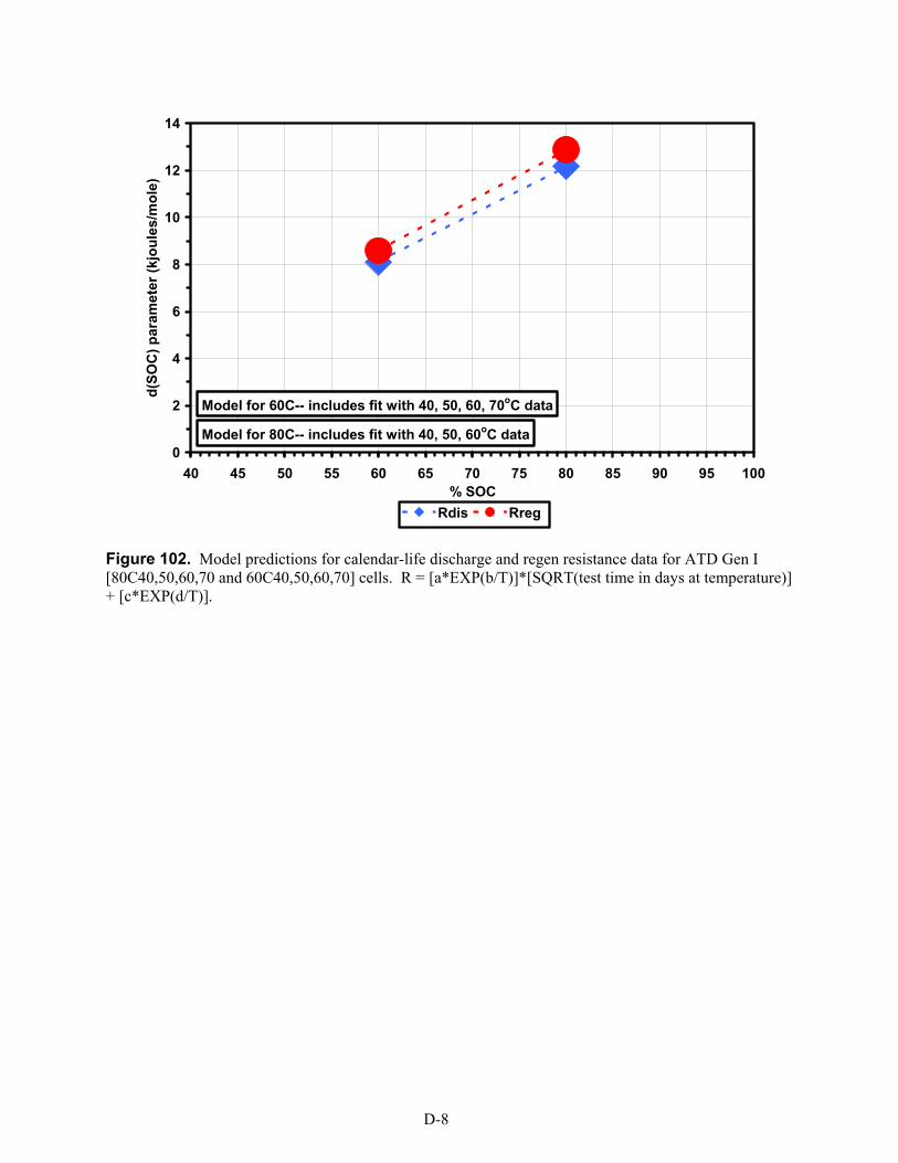
0

2

4

6

8

10

12

14

40 45 50 55 60 65 70 75 80 85 90 95 100% SOC

d(SO

C) p

aram

eter

(kjo

ules

/mol

e)

Rdis Rreg

Model for 60C-- includes fit with 40, 50, 60, 70oC data

Model for 80C-- includes fit with 40, 50, 60oC data

Figure 102. Model predictions for calendar-life discharge and regen resistance data for ATD Gen I [80C40,50,60,70 and 60C40,50,60,70] cells. R = [a*EXP(b/T)]*[SQRT(test time in days at temperature)] + [c*EXP(d/T)].

D-8

APPENDIX E

Figures from Calendar-life Discharge and Regen Resistance Tests on ATD GEN 1 Li-ION Batteries:

Leakage Current, Leakage Resistance, and Differential Capacity

0.001

0.01

0.1

1

0 0.2 0.4 0.6 0.8 1 1.2 1.4 1.6 1.8Test time (hours)

Leak

age

curr

ent (

ampe

res)

(Test #1: 4 C/1) (Test #2: 4 C/1 + RPT)(Test #3: 4 C/1 + RPT + CL40) (Test #4: 4 C/1 + RPT + CL40 + CL40)

#1 #2

#3#4

Figure 103. Leakage current following constant-current C/1 charge on ATD GEN I cell test [80C40].

1

10

100

1000

0 0.2 0.4 0.6 0.8 1 1.2 1.4 1.6 1.8Test time (hours)

Leak

age

resi

stan

ce (o

hms)

(Test #1: 4 C/1) Test #2: 4 C/1 + RPT)Test #3: 4 C/1 + RPT + CL40) (Test #4: 4 C/1 + RPT + CL40 +CL40)

#1#2

#3 #4

Figure 104. Leakage resistance following constant-current C/1 charge on ATD GEN I cell test [80C40].

E-1

3.2

3.3

3.4

3.5

3.6

3.7

3.8

3.9

4

4.1

4.2

0 0.1 0.2 0.3 0.4 0.5 0.6 0.7 0.8 0.9Charge added (ampere hours)

Cel

l vol

tage

(vol

ts)

(Test #1: 4 C/1) (Test #2: 4 C/1 + RPT)(Test #3: 4 C/1 + RPT + CL40) (Test #4: 4 C/1 + RPT + CL40 + CL40)

#1#2#3#4

Figure 105. Constant-current C/1 charge on ATD GEN I cell test [80C40].

0

0.4

0.8

1.2

1.6

2

2.4

2.8

3.2

3.6

3.4 3.5 3.6 3.7 3.8 3.9 4Cell voltage (volts)

d[C

harg

e ad

ded/

cell

capa

city

]/dV

(1/v

olt)

5 per. Mov. Avg. ((Test #1: 4 C/1))5 per. Mov. Avg. ((Test #2: 4 C/1 + RPT))5 per. Mov. Avg. ((Test #3: 4 C/1 + RPT + CL40))5 per. Mov. Avg. ((Test #4: 4 C/1 + RPT + CL40 + CL40))

Test #1Test #2

Test #3 Test #4

4.1

Figure 106. Constant-current C/1 charge on ATD GEN I cell test [80C40].

E-2

0

0.4

0.8

1.2

1.6

2

2.4

2.8

3.2

3.6

0 10 20 30 40 50 60 70 80 90 10% SOC

d[C

harg

e ad

ded/

cell

capa

city

]/dV

(1/v

olt)

5 per. Mov. Avg. ((Test #1: 4 C/1))5 per. Mov. Avg. ((Test #2: 4 C/1 + RPT))5 per. Mov. Avg. ((Test #3: 4 C/1 + RPT + CL40))5 per. Mov. Avg. ((Test #4: 4 C/1 + RPT + CL40 + CL40))

Test #1

Test #2

Test #3 Test #4

0

Figure 107. Constant-current C/1 charge on ATD GEN I cell test [80C40].

2.93

3.13.23.33.43.53.63.73.83.9

44.14.2

0 0.1 0.2 0.3 0.4 0.5 0.6 0.7 0.8 0.9 1Charge removed (ampere hours)

Cel

l vol

tage

(vol

ts)

(Test #1: 4 C/1) Test #2: 4 C/1 + RPT)(Test #3: 4 C/1 + RPT + CL40) (Test #4: 4 C/1 + RPT + CL40 + CL40)(Test #5[40C]: 4 C/1 + RPT) (Test #6[8C]: 4 C/1 + RPT)

#1#2

#3

#4

#5 [40oC]

#6 [8oC]

Figure 108. Constant-current C/1 discharge on ATD GEN I cell test [80C40].

E-3

0

0.2

0.4

0.6

0.8

1

1.2

1.4

1.6

1.8

2

2.2

3 3.1 3.2 3.3 3.4 3.5 3.6 3.7 3.8 3.9 4 4.1Cell voltage (volts)

-d[C

harg

e re

mov

ed/c

ell c

apac

ity]/d

V (1

/vol

t)

5 per. Mov. Avg. ((Test #1: 4 C/1)) 5 per. Mov. Avg. ((Test #5 [8C]: 4 C/1 + RPT))5 per. Mov. Avg. (Test #3 [40C]: 4 C/1 + RPT))

#1 [25oC]

#5 [40oC]

#6 [8oC]

Figure 109. Constant-current C/1 discharge on ATD GEN I cell test [80C40].

0

0.2

0.4

0.6

0.8

1

1.2

1.4

1.6

1.8

2

2.2

3 3.1 3.2 3.3 3.4 3.5 3.6 3.7 3.8 3.9 4 4.1Cell voltage (volts)

-d[C

harg

e re

mov

ed/c

ell c

apac

ity]/d

V (1

/vol

t)

5 per. Mov. Avg. ((Test #1: 4 C/1)) 5 per. Mov. Avg. ((Test #5 [8C]: 4 C/1 + RPT))5 per. Mov. Avg. (Test #3 [40C]: 4 C/1 + RPT))

#1 [25oC]#5 [40oC]

#6 [8oC]

Figure 110. Constant-current C/1 discharge on ATD GEN I cell test [80C40].

E-4

0

0.2

0.4

0.6

0.8

1

1.2

1.4

1.6

1.8

2

2.2

0 10 20 30 40 50 60 70 80 90 10% DOD

-d[C

harg

e re

mov

ed/c

ell c

apac

ity]/d

V (1

/vol

t)

5 per. Mov. Avg. ((Test #1: 4 C/1)) 5 per. Mov. Avg. ((Test #5 [8C]: 4 C/1 + RPT))5 per. Mov. Avg. (Test #3 [40C]: 4 C/1 + RPT))

#1 [25oC]

#5 [40oC]

#6 [8oC]

0

Figure 111. Constant-current C/1 discharge on ATD GEN I cell test [80C40].

0

0.2

0.4

0.6

0.8

1

1.2

1.4

1.6

1.8

2

2.2

3 3.1 3.2 3.3 3.4 3.5 3.6 3.7 3.8 3.9 4 4.1Cell voltage (volts)

-d[C

harg

e re

mov

ed/c

ell c

apac

ity]/d

V (1

/vol

t)

5 per. Mov. Avg. ((Test #4: 4 C/1 + RPT + CL40 + CL40))5 per. Mov. Avg. ((Test #1: 4 C/1))5 per. Mov. Avg. (Test #2: 4 C/1 + RPT + CL40))5 per. Mov. Avg. ((Test #3: 4 C/1 + RPT))

#1

#2

#4#3

Figure 112. Constant-current C/1 discharge on ATD GEN I cell test [80C40].

E-5

0

0.2

0.4

0.6

0.8

1

1.2

1.4

1.6

1.8

2

2.2

0 10 20 30 40 50 60 70 80 90 10% DOD

-d[C

harg

e re

mov

ed/c

ell c

apac

ity]/d

V (1

/vol

t)

5 per. Mov. Avg. ((Test #1: 4 C/1))5 per. Mov. Avg. ((Test #4: 4 C/1 + RPT + CL40 + CL40))5 per. Mov. Avg. (Test #2: 4 C/1 + RPT + CL40))5 per. Mov. Avg. ((Test #3: 4 C/1 + RPT))

#1

#2

#4#3

0

Figure 113. Constant-current C/1 discharge on ATD GEN I cell test [80C40].

0

0.2

0.4

0.6

0.8

1

1.2

1.4

1.6

1.8

2

2.2

0 10 20 30 40 50 60 70 80 90 10% SOC

-d[C

harg

e re

mov

ed/c

ell c

apac

ity]/d

V (1

/vol

t)

5 per. Mov. Avg. ((Test #1: 4 C/1))5 per. Mov. Avg. ((Test #4: 4 C/1 + RPT + CL40 + CL40))5 per. Mov. Avg. (Test #2: 4 C/1 + RPT + CL40))5 per. Mov. Avg. ((Test #3: 4 C/1 + RPT))

#1#2

#4 #3

0

Figure 114. Constant-current C/1 discharge on ATD GEN I cell test [80C40].

E-6

0.001

0.01

0.1

1

0 0.2 0.4 0.6 0.8 1 1.2 1.4 1.6 1.8Test time (hours)

Leak

age

curr

ent (

ampe

res)

(Test #1: 4 C/1) (Test #2: 4C/1 + RPT) (Test #3: 4 C/1 + RPT + CL70)

#2

#3

#1

Figure 115. Leakage current following constant-current C/1 charge on ATD GEN I cell test [80C70].

1

10

100

1000

0 0.2 0.4 0.6 0.8 1 1.2 1.4 1.6 1.8Test time (hours)

Leak

age

resi

stan

ce (o

hms)

(Test #1: 4 C/1) (Test #2: 4 C/1 + RPT) (Test #3: 4 C/1 + RPT + CL70)

#3

#2#1

Figure 116. Leakage resistance following constant-current C/1 charge on ATD GEN I cell test [80C70].

E-7

3.2

3.3

3.4

3.5

3.6

3.7

3.8

3.9

4

4.1

4.2

0 0.1 0.2 0.3 0.4 0.5 0.6 0.7 0.8 0.9Charge added (ampere hours)

Cel

l vol

tage

(vol

ts)

(Test #1: 4C/1) (Test #2: 4 C/1 + RPT) (Test #3: 4 C/1 + RPT + CL70)

#1#2#3

Figure 117. Constant-current C/1 charge (0.9 A) on ATD GEN I cell test [80C70].

0

0.4

0.8

1.2

1.6

2

2.4

2.8

3.2

3.6

3.4 3.5 3.6 3.7 3.8 3.9 4Cell voltage (volts)

d[C

harg

e ad

ded/

cell

capa

city

]/dV

(1/v

olt)

5 per. Mov. Avg. ((Test #2: 4 C/1 + RPT))5 per. Mov. Avg. ((Test #1: 4 C/1))5 per. Mov. Avg. ((Test #3: 4 C/1 + RPT + CL70))

Test #3

Test #1

Test #2

4.1

Figure 118. Constant-current C/1 charge on ATD GEN 1 cell test [80C70].

E-8

0

0.4

0.8

1.2

1.6

2

2.4

2.8

3.2

3.6

0 10 20 30 40 50 60 70 80 90 10% SOC

d[C

harg

e ad

ded/

cell

capa

city

]/dV

(1/v

olt)

5 per. Mov. Avg. ((Test #3: 4 C/1 + RPT CL70))5 per. Mov. Avg. ((Test #1: 4 C/1))5 per. Mov. Avg. ((Test 2: 4 C/1 + RPT))

Test #3

Test #2

Test #1

0

Figure 119. Constant-current C/1 charge on ATD GEN 1 cell test [80C70].

2.9

3

3.1

3.2

3.3

3.4

3.5

3.6

3.7

3.8

3.9

4

4.1

4.2

0 0.1 0.2 0.3 0.4 0.5 0.6 0.7 0.8 0.9 1Charge removed (ampere hours)

Cel

l vol

tage

(vol

ts)

(Test #1: 4 C/1) (Test #2: 4 C/1 + RPT) (Test #3: 4 C/1 + RPT + CL70)

#3 #2 #1

Figure 120. Constant-current C/1 discharge on ATD GEN I cell test [80C70].

E-9

0

0.2

0.4

0.6

0.8

1

1.2

1.4

1.6

1.8

2

2.2

3 3.1 3.2 3.3 3.4 3.5 3.6 3.7 3.8 3.9 4 4.1Cell voltage (volts)

-d[C

harg

e re

mov

ed/c

ell c

apac

ity]/d

V (1

/vol

t)

5 per. Mov. Avg. ((Test #1: 4C/1))5 per. Mov. Avg. ((Test #2: 4C/1 + RPT))5 per. Mov. Avg. ((Test #3: 4C/1 + RPT + CL70)

#3 #2

#1

Figure 121. Constant-current C/1 discharge on ATD GEN I cell test [80C70].

0

0.2

0.4

0.6

0.8

1

1.2

1.4

1.6

1.8

2

2.2

0 10 20 30 40 50 60 70 80 90 10% DOD

-d[C

harg

e re

mov

ed/c

ell c

apac

ity]/d

V (1

/vol

t)

5 per. Mov. Avg. ((Test #1: 4C/1))5 per. Mov. Avg. ((Test #2: 4C/1 + RPT))5 per. Mov. Avg. ((Test #3: 4C/1 + RPT + CL70)

#3

#2

#1

0

Figure 122. Constant-current C/1 discharge on ATD GEN I cell test [80C70].

E-10

0

0.2

0.4

0.6

0.8

1

1.2

1.4

1.6

1.8

2

2.2

3 3.1 3.2 3.3 3.4 3.5 3.6 3.7 3.8 3.9 4 4.1Cell voltage (volts)

-d[C

harg

e re

mov

ed/c

ell c

apac

ity]/d

V (1

/vol

t)

2 per. Mov. Avg. (Test 80C70: 4C/1 + RPT + CL70)2 per. Mov. Avg. (Test 80C40: 4C/1 + RPR + CL40 + CL40)

Figure 123. Comparison of differential capacity for [80C40] cell and a [80C70] cell for a constant current C/1 discharge. (Note that the tests conducted prior to the collection of the data are different.)

2.9

3

3.1

3.2

3.3

3.4

3.5

3.6

3.7

3.8

3.9

4

4.1

4.2

0 10 20 30 40 50 60 70 80 90 10%DOD = 100 - %SOC

Cel

l vol

tage

(vol

ts)

[C/25 Contant current discharge]

0

Figure 124. ANL calibration curve for ATD GEN I Li-Ion cells.

E-11

0

0.2

0.4

0.6

0.8

1

1.2

1.4

1.6

1.8

2

3 3.1 3.2 3.3 3.4 3.5 3.6 3.7 3.8 3.9 4 4.1Cell voltage (volts)

-d[C

harg

e re

mov

ed/c

ell c

apac

ity]/d

V (1

/vol

t)

Figure 125. Constant current C/25 discharge of ANL ATD Gen 1 calibration data. (Differential capacity as a function of cell voltage.)

0

0.2

0.4

0.6

0.8

1

1.2

1.4

1.6

1.8

2

0 10 20 30 40 50 60 70 80 90 10% DOD

-d[C

harg

e re

mov

ed/c

ell c

apac

ity]/d

V (1

/vol

t)

0

Figure 126. Constant current C/25 discharge of ANL ATD Gen 1 calibration data. (Differential capacity as a function of %DOD.)

E-12

2.9

3

3.1

3.2

3.3

3.4

3.5

3.6

3.7

3.8

3.9

4

4.1

4.2

0 0.1 0.2 0.3 0.4 0.5 0.6 0.7 0.8 0.9 1Charge removed (Ah)

Volta

ge (v

olts

)

New

Aged to Failure

Figure 127. Constant current C/25 discharge on ATD GEN I cell test [60960].

0

0.2

0.4

0.6

0.8

1

1.2

1.4

1.6

1.8

2

3 3.1 3.2 3.3 3.4 3.5 3.6 3.7 3.8 3.9 4 4.1Cell voltage (volts)

-d[C

harg

e re

mov

ed/c

ell c

apac

ity]/d

V(1

/vol

t)

ANL Calibration (C/25)100 per. Mov. Avg. (Aged to Failure (C/25))100 per. Mov. Avg. (New (C/25))

NewAged to Failure

Figure 128. Constant current C/25 discharge comparison of ANL ATD Gen 1 calibration data with a [60960] test cell.

E-13

E-14

0

0.2

0.4

0.6

0.8

1

1.2

1.4

1.6

1.8

2

0 10 20 30 40 50 60 70 80 90 10% DOD

-d[C

harg

e re

mov

ed/c

ell c

apac

ity]/d

V(1

/vol

t)

ANL Calibration (C/25)100 per. Mov. Avg. (Aged to Failure (C/25))100 per. Mov. Avg. (New (C/25))

NewAged to Failure

0

Figure 129. Constant current C/25 discharge comparison of ANL ATD Gen 1 calibration data with a [60960] test cell.