1

Calibration of a Quartz Tuning Fork for Low Temperature

Measurements

Joshua Wiman

Mentor: Yoonseok Lee

University of Florida

Mechanical oscillators are commonly used to measure the properties of cryogenic liquids.

Commercial quartz tuning forks have shown promise as viscometers and thermometers for low

temperature experiments. These forks are inexpensive, easy to install, and insensitive to magnetic fields.

Before a fork can be used, it must be calibrated against a hydrodynamic model. This model is found to be

accurate for liquid 4He at least down to a temperature of 1.5 K. An experiment similar to this one will be

incorporated into the University of Florida Advanced Physics Lab 2.

I. Introduction

Studies of the properties and behavior of cryogenic fluids can be done using a mechanical

oscillator immersed in the fluid. Through use of a hydrodynamic model [1], changes in the

oscillator’s amplitude, resonance frequency, and resonance width can be used to infer the

temperature, density, or viscosity of the surrounding fluid. However, the oscillator must first be

calibrated against a fluid where density and viscosity are known as functions of temperature. In

this study, we calibrated a commercial tuning fork against liquid 4He and compared our data with

the hydrodynamic model.

Common mechanical oscillators include wires, spheres, and, more recently, tuning forks.

Commercial quartz tuning forks typically measure less than 4 mm in length and are vacuum

sealed in a metal canister; these forks are designed to provide reliable timing for watches and

2

other small devices through a calibrated resonance frequency usually near 215

Hz = 32.768 kHz

[1]. To drive oscillations, an alternating voltage is applied across two electrodes plated on the

prongs of the fork; the piezoelectric effect converts these mechanical oscillations into electrical

current which can be easily measured.

The quartz tuning fork has several advantages and disadvantages over wires and spheres.

First, tuning forks are inexpensive and can be installed by simply opening the metal canister and

connecting the two provided electrode leads. Second, individual forks can be calibrated through

only three parameters from resonance curve measurements in vacuum and in a fluid of known

density and viscosity. Finally, forks do not require a magnetic field for operation and are

generally insensitive to the presence of such a field [2]. On the other hand, due to their novelty

and more complex geometry, far less theoretical information is available on the behavior of such

forks in viscous fluids [1]. Also, forks can differ significantly from one model to another and

even between samples of the same model; hence, each individual fork must be calibrated before

use [1].

To calibrate the fork, we measured current, resonance frequency, and resonance width in

liquid 4He down to a temperature of 1.5 K. Our primary goal was to test the validity of quartz

tuning forks as thermometers and viscometers in cryogenic fluids and to identify any potential

difficulties with obtaining reliable measurements.

II. Theory

1. Fork in Vacuum

We used the model of Blaauwgeers et al. [1] to relate the fork response to the properties

of the surrounding fluid. As this model depends on the properties of the fork in vacuum, we first

3

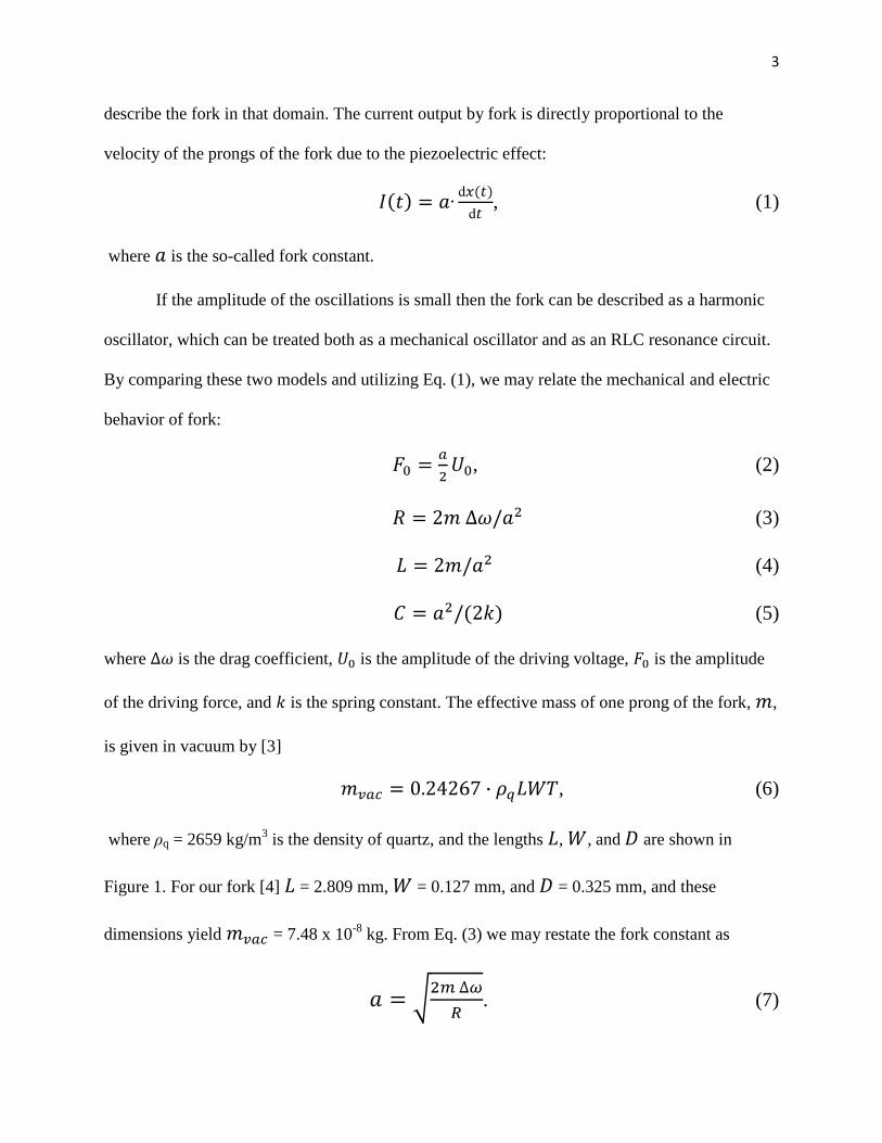
describe the fork in that domain. The current output by fork is directly proportional to the

velocity of the prongs of the fork due to the piezoelectric effect:

, (1)

where is the so-called fork constant.

If the amplitude of the oscillations is small then the fork can be described as a harmonic

oscillator, which can be treated both as a mechanical oscillator and as an RLC resonance circuit.

By comparing these two models and utilizing Eq. (1), we may relate the mechanical and electric

behavior of fork:

, (2)

(3)

(4)

(5)

where is the drag coefficient, is the amplitude of the driving voltage, is the amplitude

of the driving force, and is the spring constant. The effective mass of one prong of the fork, ,

is given in vacuum by [3]

, (6)

where ρq = 2659 kg/m3 is the density of quartz, and the lengths , , and are shown in

Figure 1. For our fork [4] = 2.809 mm, = 0.127 mm, and = 0.325 mm, and these

dimensions yield = 7.48 x 10-8

kg. From Eq. (3) we may restate the fork constant as

. (7)

4

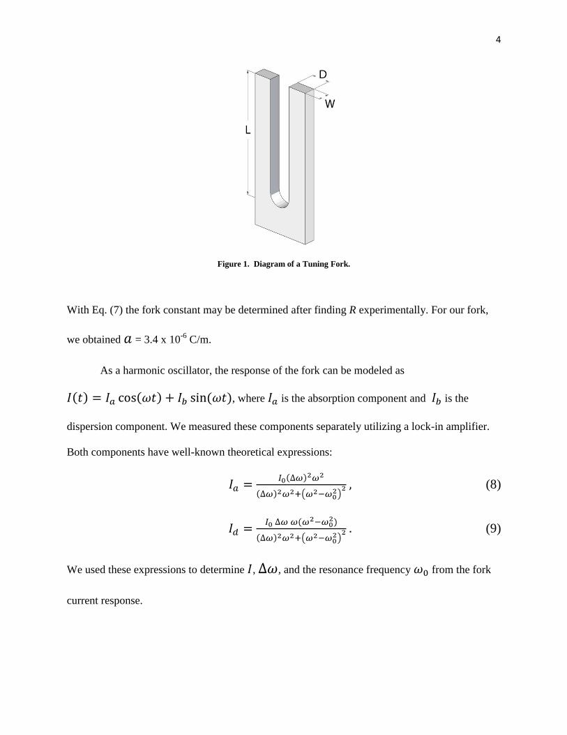
Figure 1. Diagram of a Tuning Fork.

With Eq. (7) the fork constant may be determined after finding R experimentally. For our fork,

we obtained = 3.4 x 10-6

C/m.

As a harmonic oscillator, the response of the fork can be modeled as

, where is the absorption component and is the

dispersion component. We measured these components separately utilizing a lock-in amplifier.

Both components have well-known theoretical expressions:

(8)

(9)

We used these expressions to determine , , and the resonance frequency from the fork

current response.

5

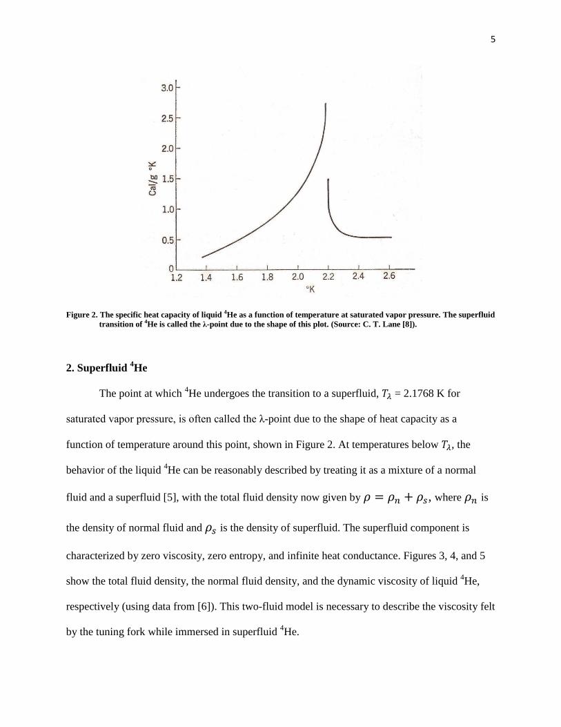
Figure 2. The specific heat capacity of liquid 4He as a function of temperature at saturated vapor pressure. The superfluid

transition of 4He is called the λ-point due to the shape of this plot. (Source: C. T. Lane [8]).

2. Superfluid 4He

The point at which 4He undergoes the transition to a superfluid, = 2.1768 K for

saturated vapor pressure, is often called the λ-point due to the shape of heat capacity as a

function of temperature around this point, shown in Figure 2. At temperatures below , the

behavior of the liquid 4He can be reasonably described by treating it as a mixture of a normal

fluid and a superfluid [5], with the total fluid density now given by , where is

the density of normal fluid and is the density of superfluid. The superfluid component is

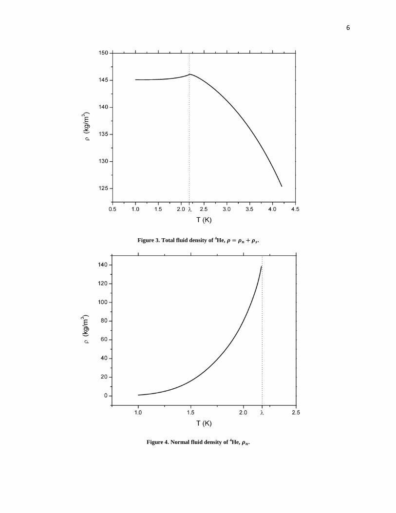
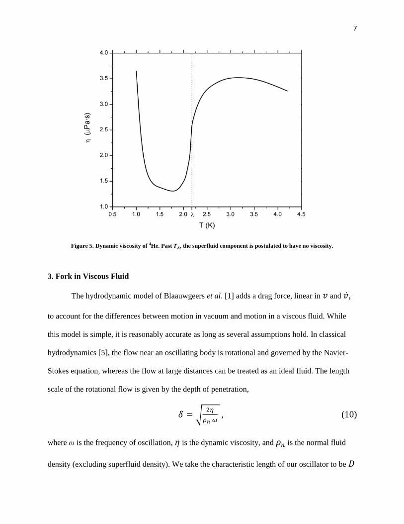
characterized by zero viscosity, zero entropy, and infinite heat conductance. Figures 3, 4, and 5

show the total fluid density, the normal fluid density, and the dynamic viscosity of liquid 4He,

respectively (using data from [6]). This two-fluid model is necessary to describe the viscosity felt

by the tuning fork while immersed in superfluid 4He.

6

Figure 3. Total fluid density of 4He, .

Figure 4. Normal fluid density of 4He, .

7

Figure 5. Dynamic viscosity of 4He. Past , the superfluid component is postulated to have no viscosity.

3. Fork in Viscous Fluid

The hydrodynamic model of Blaauwgeers et al. [1] adds a drag force, linear in and ,

to account for the differences between motion in vacuum and motion in a viscous fluid. While

this model is simple, it is reasonably accurate as long as several assumptions hold. In classical

hydrodynamics [5], the flow near an oscillating body is rotational and governed by the Navier-

Stokes equation, whereas the flow at large distances can be treated as an ideal fluid. The length

scale of the rotational flow is given by the depth of penetration,

(10)

where ω is the frequency of oscillation, is the dynamic viscosity, and is the normal fluid

density (excluding superfluid density). We take the characteristic length of our oscillator to be

8

and require that and , where is the oscillation amplitude. This requirement

ensures that the rotational flow is restricted to only a small layer near the surface of the

oscillator. From the known properties of liquid He4 [6], we estimate to be on the order of 0.1

μm for an oscillation frequency of 32 kHz, clearly less than = 0.325 mm. We also note that, at

this frequency, a velocity of over 1 m/s would be necessary to violate ; we kept the

velocity below 1 cm/s for this experiment.

If the preceding conditions are satisfied, then it is reasonably valid to model the oscillator

system with the drag force

, (11)

where represents drag and represents mass enhancement. The coefficient is found by

solving the potential flow problem around the fork:

(12)

where is a coefficient related to the fork geometry, is the surface area of a

leg of the fork, and is the volume of rotational flow. The mass enhancement is given

by

, (13)

where both and are geometrical coefficients, is the volume of a single prong,

and is the total fluid density. In Eq. (13), the first term accounts for the fluid displaced by the

body, while the second term accounts for fluid moving in comotion with the body.

By adding to the vacuum equation of motion and simplifying, we obtain the

following relations:

9

(14)

. (15)

Note that a term in Eq. (15) dependent on has been removed due to its negligible

magnitude. Eqs. (14) and (15) can be used to determine , and if and are known.

Finally, once these coefficients have been found the tuning fork can be used to measure and .

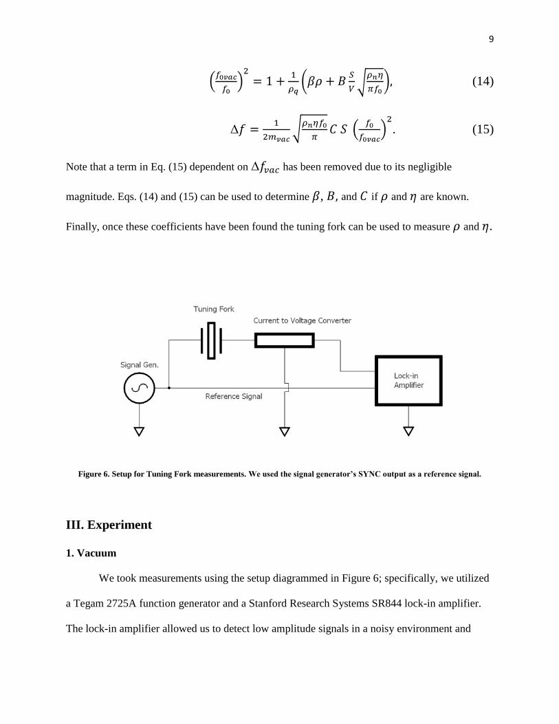
Figure 6. Setup for Tuning Fork measurements. We used the signal generator’s SYNC output as a reference signal.

III. Experiment

1. Vacuum

We took measurements using the setup diagrammed in Figure 6; specifically, we utilized

a Tegam 2725A function generator and a Stanford Research Systems SR844 lock-in amplifier.

The lock-in amplifier allowed us to detect low amplitude signals in a noisy environment and

10

separate those signals into components in-phase and out-of-phase with the function generator. To

determine the resonance properties of the fork at a given time, we slowly varied the frequency of

the function generator and collected the lock-in output as a function of frequency. We fixed the

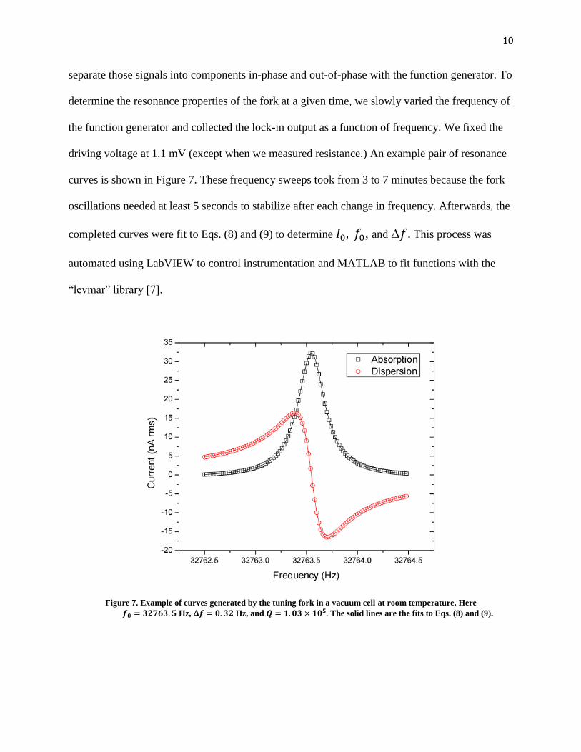
driving voltage at 1.1 mV (except when we measured resistance.) An example pair of resonance

curves is shown in Figure 7. These frequency sweeps took from 3 to 7 minutes because the fork

oscillations needed at least 5 seconds to stabilize after each change in frequency. Afterwards, the

completed curves were fit to Eqs. (8) and (9) to determine , and . This process was

automated using LabVIEW to control instrumentation and MATLAB to fit functions with the

“levmar” library [7].

Figure 7. Example of curves generated by the tuning fork in a vacuum cell at room temperature. Here Hz, Hz, and The solid lines are the fits to Eqs. (8) and (9).

11

Throughout this experiment we used only a single tuning fork [4]; this fork was opened

to the environment by cutting off the top of the canister using a lathe. We first tested this fork in

vacuum at room temperature and ~77K to determine , , R and , given in Table I.

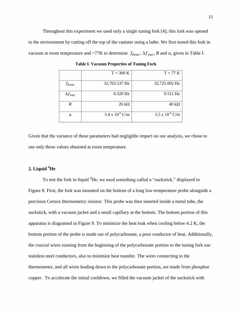
Table I. Vacuum Properties of Tuning Fork

T = 300 K T = 77 K

32,763.537 Hz 32,725.002 Hz

0.320 Hz 0.511 Hz

R 26 k 40 k

3.4 x 10-6

C/m 3.5 x 10-6

C/m

Given that the variance of these parameters had negligible impact on our analysis, we chose to

use only those values obtained at room temperature.

2. Liquid 4He

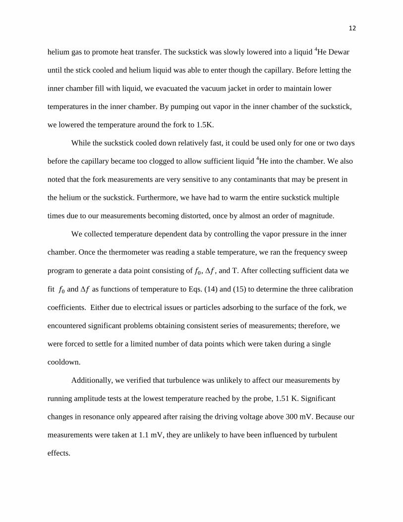
To test the fork in liquid 4He, we used something called a “suckstick,” displayed in

Figure 8. First, the fork was mounted on the bottom of a long low-temperature probe alongside a

precision Cernox thermometry resistor. This probe was then inserted inside a metal tube, the

suckstick, with a vacuum jacket and a small capillary at the bottom. The bottom portion of this

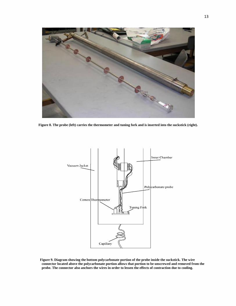
apparatus is diagramed in Figure 9. To minimize the heat leak when cooling below 4.2 K, the

bottom portion of the probe is made out of polycarbonate, a poor conductor of heat. Additionally,

the coaxial wires running from the beginning of the polycarbonate portion to the tuning fork use

stainless steel conductors, also to minimize heat transfer. The wires connecting to the

thermometer, and all wires leading down to the polycarbonate portion, are made from phosphor

copper. To accelerate the initial cooldown, we filled the vacuum jacket of the suckstick with

12

helium gas to promote heat transfer. The suckstick was slowly lowered into a liquid 4He Dewar

until the stick cooled and helium liquid was able to enter though the capillary. Before letting the

inner chamber fill with liquid, we evacuated the vacuum jacket in order to maintain lower

temperatures in the inner chamber. By pumping out vapor in the inner chamber of the suckstick,

we lowered the temperature around the fork to 1.5K.

While the suckstick cooled down relatively fast, it could be used only for one or two days

before the capillary became too clogged to allow sufficient liquid 4He into the chamber. We also

noted that the fork measurements are very sensitive to any contaminants that may be present in

the helium or the suckstick. Furthermore, we have had to warm the entire suckstick multiple

times due to our measurements becoming distorted, once by almost an order of magnitude.

We collected temperature dependent data by controlling the vapor pressure in the inner

chamber. Once the thermometer was reading a stable temperature, we ran the frequency sweep

program to generate a data point consisting of , , and T. After collecting sufficient data we

fit and as functions of temperature to Eqs. (14) and (15) to determine the three calibration

coefficients. Either due to electrical issues or particles adsorbing to the surface of the fork, we

encountered significant problems obtaining consistent series of measurements; therefore, we

were forced to settle for a limited number of data points which were taken during a single

cooldown.

Additionally, we verified that turbulence was unlikely to affect our measurements by

running amplitude tests at the lowest temperature reached by the probe, 1.51 K. Significant

changes in resonance only appeared after raising the driving voltage above 300 mV. Because our

measurements were taken at 1.1 mV, they are unlikely to have been influenced by turbulent

effects.

13

Figure 8. The probe (left) carries the thermometer and tuning fork and is inserted into the suckstick (right).

Figure 9. Diagram showing the bottom polycarbonate portion of the probe inside the suckstick. The wire

connector located above the polycarbonate portion allows that portion to be unscrewed and removed from the

probe. The connector also anchors the wires in order to lessen the effects of contraction due to cooling.

14

IV. Results and Conclusion

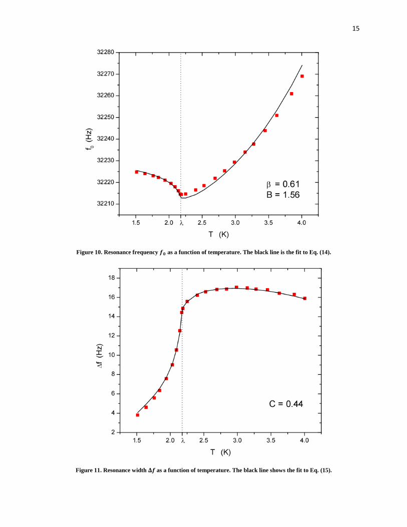
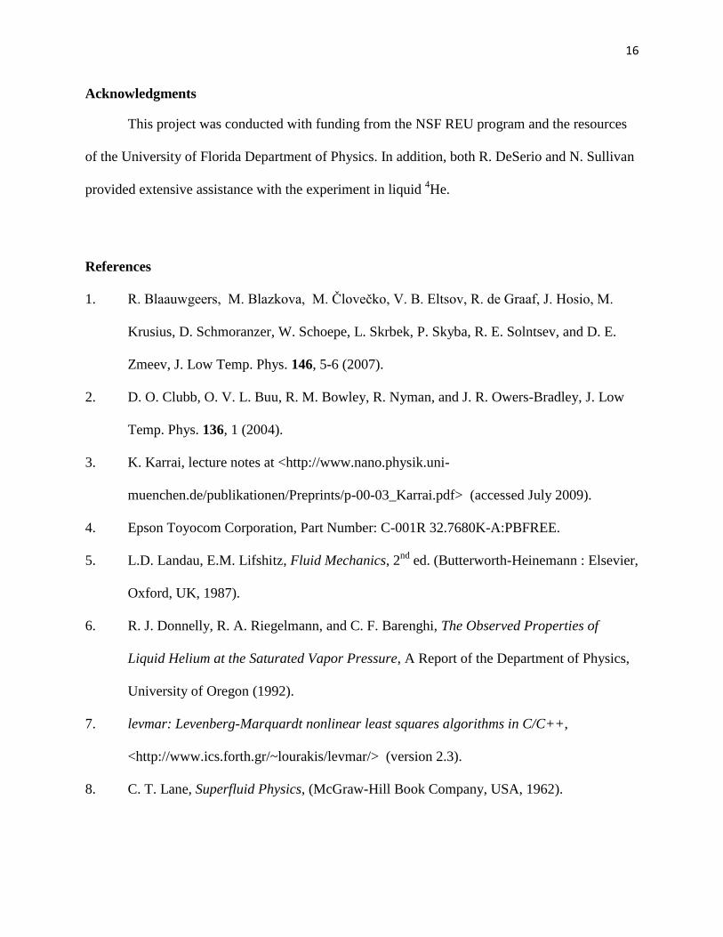
The results of our experiment in liquid 4He are shown in Figures 10 and 11. Both and

are quite sensitive to the properties of the surrounding fluid; in particular, both show clear

changes after the lambda point. Clearly, Eqs. (14) and (15) are reasonably good descriptions of a

tuning fork in liquid 4He. However, it remains to be seen whether or not they will remain

accurate below 1K. If this model remains predictive, then the quartz tuning fork could serve as a

low temperature thermometer and viscometer that is both easy to install and requires no magnetic

field to operate.

15

Figure 10. Resonance frequency as a function of temperature. The black line is the fit to Eq. (14).

Figure 11. Resonance width as a function of temperature. The black line shows the fit to Eq. (15).

16

Acknowledgments

This project was conducted with funding from the NSF REU program and the resources

of the University of Florida Department of Physics. In addition, both R. DeSerio and N. Sullivan

provided extensive assistance with the experiment in liquid 4He.

References

1. R. Blaauwgeers, M. Blazkova, M. Človečko, V. B. Eltsov, R. de Graaf, J. Hosio, M.

Krusius, D. Schmoranzer, W. Schoepe, L. Skrbek, P. Skyba, R. E. Solntsev, and D. E.

Zmeev, J. Low Temp. Phys. 146, 5-6 (2007).

2. D. O. Clubb, O. V. L. Buu, R. M. Bowley, R. Nyman, and J. R. Owers-Bradley, J. Low

Temp. Phys. 136, 1 (2004).

3. K. Karrai, lecture notes at <http://www.nano.physik.uni-

muenchen.de/publikationen/Preprints/p-00-03_Karrai.pdf> (accessed July 2009).

4. Epson Toyocom Corporation, Part Number: C-001R 32.7680K-A:PBFREE.

5. L.D. Landau, E.M. Lifshitz, Fluid Mechanics, 2nd

ed. (Butterworth-Heinemann : Elsevier,

Oxford, UK, 1987).

6. R. J. Donnelly, R. A. Riegelmann, and C. F. Barenghi, The Observed Properties of

Liquid Helium at the Saturated Vapor Pressure, A Report of the Department of Physics,

University of Oregon (1992).

7. levmar: Levenberg-Marquardt nonlinear least squares algorithms in C/C++,

<http://www.ics.forth.gr/~lourakis/levmar/> (version 2.3).

8. C. T. Lane, Superfluid Physics, (McGraw-Hill Book Company, USA, 1962).