1

California Natural and Working Lands Carbon and Greenhouse Gas Model (CALAND)

Version 3, December 2018

Technical Documentation

Alan Di Vittorio and Maegen B. Simmonds Lawrence Berkeley National Laboratory

2

California Natural and Working Lands Carbon and Greenhouse Gas Model (CALAND)

Contents

1. Summary .................................................................................................................... 3

2. Model structure ......................................................................................................... 6

2.1 Initial state ............................................................................................................ 9

2.1.1. Land categories ............................................................................................. 9

2.1.2. Biomass carbon ........................................................................................... 10

2.1.3. Soil organic carbon ...................................................................................... 11

2.2. Projection methods .......................................................................................... 12

2.2.1. Net ecosystem carbon exchange ................................................................. 15

2.2.2. Mortality rates .............................................................................................. 19

2.2.3. Climate effects ............................................................................................ 19

2.2.4. Management effects ................................................................................... 20

2.2.5. Forest management ..................................................................................... 24

2.2.6. Wildfire ......................................................................................................... 26

2.2.7. Land type conversion ................................................................................... 28

3. Model outputs and diagnostics .............................................................................. 32

4. Baseline and alternative land use and management scenarios for the Natural andWorking Lands Climate Change Implementation Plan………………………………33

5. Looking Ahead ........................................................................................................ 35

Appendices .................................................................................................................. 36 Appendix A: Land categories identified for use in CALAND ........................................ 37 Appendix B: Annual net carbon exchange in live vegetation and soil under historic

climate.. .................................................................................................................. 40 Appendix C: Annual net mortality fractions of live biomass carbon ............................. 45 Appendix D: Grassland, Savanna, Woodland, and Cultivated land management ...........

enhancement factors for soil carbon exchange ...................................................... 50 Appendix E: Forest management enhancement/reduction factors for vegetation and

soil carbon exchange (sans mortality), mortality, and wildfire severity .................... 51 Appendix F1: Forest biomass carbon transfer fractions due to harvest. ..................... 63 Appendix F2: Forest biomass carbon transfer fractions due to fuel reduction ................

activities... .............................................................................................................. 64 Appendix F3: Forest biomass carbon transfer fractions due to conversion to Cultivated

Land or Urban Area. ............................................................................................... 66 Appendix G: CALAND Output variables and definitions (214 variables) ...................... 67

References ................................................................................................................... 80

Extended Bibliography for CALAND .......................................................................... 86

3

1. Summary

The California Natural and Working Lands Carbon and Greenhouse Gas Model (CALAND) is

an empirically-based carbon accounting model that simulates the effects of various

management practices and land use or land cover change on carbon dynamics in all California

lands, including land-atmosphere carbon dioxide (CO2) exchange, and emissions of methane

(CH4) and black carbon (BC, optional) associated with wetlands function and biomass burning,

respectively, and the global warming potential (GWP) of net emissions of these three

greenhouse gases (GHGs).1 Starting with historical carbon stock and flux data and two options

for historical land use/cover change,2 CALAND simulates annual carbon stocks and fluxes,

including material flow to wood products and bioenergy, for given land use/management

scenarios from 2010 through 2100. The potential effects of climate change on carbon dynamics

and wildfire are optional, with three choices: historical (no climate change effects),

Representative Concentration Pathway (RCP) 4.5, or RCP 8.5.

CALAND’s primary function is to quantify the difference between expected net GHG

emissions from a historically grounded, baseline land use and management scenario and net

GHG emissions arising from alternative land use and management activities pursued on a range

of spatiotemporal scales. This comparison will quantify the change in net GHG emissions that

is expected to arise from applied land conservation and management activities, relative to the

reference baseline. The alternative management scenarios developed for the Natural and

Working Lands Climate Change Implementation Plan were developed in 2018. Currently,

CALAND should be used only to examine differences between GHG emissions arising from

the baseline and alternative scenarios, as opposed to absolute GHG emissions.3

CALAND operates statewide on 940 land type categories plus ocean seagrass (Table 1, Figure 1).4 CALAND simulates one scenario at a time to generate a single output file using two input data files and one processing script (caland.r). The output file is an Excel workbook containing several tables as individual sheets. The two input files are also Excel workbooks, which contain

1Version 1 (November 2016) did not include these greenhouse gas outputs. Version 2 (October 2017)

did not have the option to output only carbon dioxide and methane emissions. 2The default option is land –use-change driven data from the CA Fourth Climate Assessment, and the

alternative is remote sensing based change data from 2001-2010. Previous versions used only the

remote-sensing based data.

3Currently, the absolute outputs for any individual scenario are not robust due to extremely high

uncertainty of historical baseline land use/cover change, combined with unknown distribution and

carbon dynamics of savanna/woodland with woody versus grass understory. Planned updates to the

historical baseline using a land use change driven approach may improve absolute carbon

projections, but do not address non-anthropogenic land cover change or data limitations for

particular land types. Uncertainties in initial carbon density and net ecosystem carbon exchange are

better quantified, but also dramatically affect absolute projections. 4Version 1 had 45 land categories with 15 land types and three ownership classes.

4

the model data and scenario, respectively. The model data are constant across compared scenarios and comprise an integration of many data sources for carbon densities, fluxes, land management, land conversion, and fire. These data sources are described here and detailed in the appendices to this report. Each scenario prescribes the initial landscape state and annual areas of land cover change, management, and wildfire, along with climate scaling factors and annual mortality rates for vegetation. Each scenario is defined in its own input file. Due to the complexity of the input file, there is a function (write_caland_inputs.r) that reads raw data and generates the input file. Most of these raw data are given, but the user must create a raw scenario input file that defines one or more management scenarios. The raw scenario input file can use either acres or hectares as the area units, and these are converted to hectares by the write_caland_inputs function. There is a primary diagnostic plotting function (plot_caland.r) for creating figures from two or more scenario outputs, and two additional functions (plot_scen_types.r, plot_uncertainty.r) to create additional plots (see Section 3). All functions are implemented in R (www.r-project.org).

Table 1: Land Category Delineations The 940 land categories are defined by the intersection of nine ownership classes, nine spatial regions, and 15 land types. Seagrass is offshore and is assigned to the coastal region and other federally owned lands. (See Appendix B for definitions).

Spatial Regions Ownership Classes Land Cover Types

Central Coast U.S. Bureau of Land Management

Barren Savanna

Central Valley National Park Service Cultivated Land Seagrass

Sacramento-San Joaquin Delta

U.S. Department of Defense

Desert Shrubland

Deserts USDA Forest Service (non-wilderness)

Forest Sparse

Eastside Other Federal Government5

Fresh Marsh Coastal Marsh

Klamath State Government Grassland Urban Area

North Coast Local Government Ice Water

Sierra Cascades Private Meadow Woodland

South Coast Conservation Easement Protected

5U.S.Bureau of Indian Affairs, U.S. Bureau of Reclamation, U.S. Fish and Wildlife Service, USDA

Forest Service Wilderness Area, and other Federal lands

5

Figure 1: CALAND Land Categories Corresponding to Table 1. The land categories are defined by the intersection of nine spatial regions (delineated by white lines), a) 15 land cover types, and b) nine ownership classes. Seagrass is considered separately.

a) 15 land cover types

6

b) Nine ownership classes

2. Model structure

CALAND is an empirically-based database model that projects the accumulation and fate

of above- and below-ground carbon in up to seven carbon pools (Table 2); carbon flow to

wood products and bioenergy; and emissions of CO2, CH4, and BC, for a given set of land

categories, under a variety of management activities. By default, CALAND outputs only

CO2 and CH4 emissions, while still tracking the amount of BC that could be emitted (this

small BC fraction is emitted as CO2). Optionally, BC can be emitted separately with its

corresponding GWP of 900. CALAND relies on California-specific data from academic

literature, state institutions, and state partner organizations. It simulates carbon stocks and

7

fluxes among several pools based on explicit environmental and human processes; as such

it is an IPCC Tier 3 approach for estimating landscape carbon dynamics. The data consist

of carbon densities, rates of net carbon accumulation or emissions to the atmosphere, the

proportion of CO2, CH4, and BC in carbon emissions from burned biomass, and the effects

of forest management, land conversion, and fire on carbon stocks and fates. These data are

provided in various formats and represent places ranging from specific study sites to

general land types (e.g., Forest). As such, these data are processed into averages or

characteristic values for each of 940 land categories—the intersection of 15 land types,

nine ownership classes, and nine regions (Table 1, Figure 1)—and one Seagrass category,

along with uncertainty ranges for the carbon data. Table 2: Carbon Pools Represented in CALAND Boxes marked by “X” indicate carbon pools included in CALAND. Seagrass starts with non-zero area and zero carbon, and Fresh Marsh starts with zero area and zero carbon.

The impacts of management on landscape carbon are estimated by taking the difference

between a management scenario and a baseline scenario simulated by CALAND. Baseline

scenarios are often extrapolations of recent trends but can also represent the absence of

mangement6 to estimate the total effects of a management scenario. The California Natural

Resources Agency has provided two management scenarios and one non-management

baseline scenario that are in accordance with the Natural and Working Lands

Implementation Plan (section 2.2). Each simulation starts from an initial condition in 2010

and calculates one year at a time based on the given scenario.

6 Includes only wildfire, mortality, ecosystem carbon fluxes, historical land use and cover

change, and optional climate change effects.

8

Figure 2 illustrates the relationships between model components. The model starts with an

initial carbon and land cover state in 2010 and simulates the following processes on an annual

time step:

1. The net ecosystem carbon accumulation or loss (including adjustments based on

climate and/or management activities),

2. The effects of forest management on carbon stocks, including carbon storage in

wood products (without changing the land type area),

3. The effects of wildfire on landscape carbon (with optional non-regeneration of some

high severity burn area),

4. The effects of changes in land type area on landscape carbon (including restoration

activities and wood products from forest to urban/agriculture conversion)

Management activities for Cultivated Land, Rangeland (Grassland, Savanna, Woodland),

Forest (indirect effects on growth, mortality, and soil), and Urban Area (urban forest

fraction) are implemented in step (1). Forest management (including dead removal from

Urban Area) is directly implemented in step (2). Restoration, Land protection, and Forest

expansion are implemented in step (4). The carbon densities for all pools are updated after

each group of related processes (1)-(4). All landscape carbon, accumulated or emitted, and

carbon stored or emitted by wood products, is accounted for (i.e., carbon is conserved). All

landscape carbon exchange, except for decay of wildfire-killed biomass, is assumed to occur

within the same year of the driving activity. This includes, for example, decay of logging

residue that has been removed from the forest and soil carbon loss due to land conversion.

Land-atmosphere exchange of CO2, CH4, and BC, including carbon emission pathways for

discarded wood products and bioenergy generation from forest biomass, are calculated from

the carbon dynamics after all years have been processed.

Figure 2: CALAND Model Operation The CALAND model operates on an annual time step.

9

2.1 Initial state

The initial land cover and biomass carbon state begins in 2010 and is derived from the

improved California Air Resources Board (CARB) Greenhouse Gas Inventory for California Forests and Other Lands (CARB Inventory; Saah et al., 2016; Battles et al.,

2014) and an urban forest assessment (McPherson et al, 2017). The initial soil carbon state is derived from the NRCS gSSURGO database (USDA, 2014) and a review of California

rangeland soil studies (Silver et al., 2010). These data have been processed with the aid of a geographic information system so that they are geographically aligned7 in order to obtain

average carbon density values and associated uncertainty for the 940 land categories. The mean, standard deviation, maximum, and minimum carbon densities for each land

category (for up to six biomass pools and one soil pool) are included in the carbon input file. Uncertainty in CALAND inputs is consistently characterized as the standard deviation

of the calculated mean values because not all data include explicit uncertainty.

2.1.1. Land categories

The land categories are the spatial units for which changes in landscape carbon are calculated. They are defined by the intersection of land cover types, ownership classes, and spatial regions. The land cover data used to delineate the 15 land types in CALAND are based on remote sensing data from the LANDFIRE program8 and are provided in the CARB Inventory database (Saah et al., 2016, Battles et al., 2014). The 204 (2010) LANDFIRE land cover types for California are aggregated into 15 CALAND land types based on the 2008 classification scheme provided in the CARB Inventory. These 15 land types are intersected spatially with nine ownership classes derived from a combination of CAL FIRE Fire Resource and Assessment Program (FRAP) ownership data,9 the 2015 California Conservation Easement Database (CCED),10 and USFS wilderness area data;11 and nine spatial regions derived from a combination of the USFS Pacific Southwest Region12 ecological subregions for the state of California, the Sacramento-San Joaquin Legal Delta boundary (as defined by the Delta Protection Act of 1959), and the Suisun

7 GRASS GIS 7.0. All the spatial data have been transformed to CA Teale Equal Area Albers

projection at 30 m resolution with extent: 736072.75860325 to 613987.24139675 south-north

and -423161.42973785 to 586578.57026215 west-east. 8 LANDFIRE data available online: https://www.landfire.gov 9 CAL FIRE FRAP Mapping – FRAP Data available online:

http://frap.fire.ca.gov/data/frapgisdata- sw-ownership13_2_download;

California Multi-Source Land Ownership available online:

http://frap.fire.ca.gov/data/statewide/FGDC_metadata/ownership13_2.xml 10 CCED, 2015 11 USDA Forest Service FSGeodata Clearinghouse available online:

https://data.fs.usda.gov/geodata/edw/datasets.php;

https://data.fs.usda.gov/geodata/edw/edw_resources/meta/S_USA.Wilderness.xml

10

Marsh as determined by soil carbon densities greater than 250 Mg C ha-1. The spatial

regions are the aggregation of Level 2 ecological subregions recommended by CAL FIRE

(Figure A1 in Appendix A; also defined in the 2018 California Forest Carbon Plan13),

modified to delineate the Legal Delta and Suisun Marsh. The Delta region has been

extracted from the Central Valley region, with some adjustments along the border with the

Central Coast (<2km), to ensure complete inclusion of the Legal Delta and distinct regions

with contiguous area. This delineation will facilitate modeling of wetlands management

and restoration practices that are unique to the Delta region. Fresh Marsh is a unique

category that is not represented in the LANDFIRE data classification (i.e. area = 0), yet it

is included in order to track managed wetland restoration in the Sacramento-San Joaquin

Delta. The initial area of offshore Seagrass is the midpoint value of the range reported by

the West Coast Region of NOAA Fisheries (NOAA, 2014).

2.1.2 Biomass carbon

The initial 2010 biomass carbon density values for all land categories (except Urban Area)

are from the CARB Inventory database (Saah et al., 2016, Battles et al., 2014), which does

not include soil carbon. These source data are stored on a 30 m resolution grid, with distinct

biomass values for each of the 204 LANDFIRE land cover types. They are calibrated to

USFS FIA data and available literature. The biomass values were converted to carbon

values using the recommended factor (carbon = 0.47*biomass; Saah et al., 2016). These

carbon values were used to calculate the area- weighted average of the grid cell values

within each land category, which is the primary input carbon density to CALAND. The

standard deviation, maximum, and minimum of these grid cells are also available in the

carbon input file. The Urban Area input carbon densities come directly from the source

data for the CARB Inventory database, with regional values split into aboveground (72%)

and belowground (28%) main tree canopy carbon (McPherson et al., 2017).14 The six

biomass carbon pools are aboveground main canopy, belowground main canopy (root),

understory, standing dead, downed dead, and litter (Table 2).

Other sources were considered for gridded initial biomass carbon, but they covered only

the forested area and were based on USFS FIA data. Specifically, a 250 m resolution data

set (Wilson et al., 2013) was compared to the CARB Inventory data for 45 land categories.

12 USDA Forest Service Pacific Southwest Region State-Level Datasets available online:

https://www.fs.usda.gov/detail/r5/landmanagement/gis/?cid=STELPRDB5327836;

https://www.fs.usda.gov/detail/r5/landmanagement/gis/?cid=fsbdev3_048133 13 California Forest Carbon Plan available online; page 66: http://resources.ca.gov/wp-

content/uploads/2018/05/California-Forest-Carbon-Plan-Final-Draft-for-Public-Release-May-

2018.pdf 14 Previous versions assigned all of the reported statewide value to aboveground carbon, across

all regions.

11

Relatively small differences were found between the Forest land types, but there was an

apparent overestimation of carbon density for the other land types in the coarser data due

to limited coverage and mixing of Forest with less vegetated area.

In most cases, CALAND’s average, aggregated carbon density values are comparable to

other reported estimates, especially considering the differences in aggregation and

categories (Forest: Birdsey et all, 2002; FRAP, 2010; Hudiburg et al., 2009; Pearson et al.,

2009. Desert: Evans et al., 2014. Grassland: Ryals et al. 2013. Cultivated Land: Brown et

al., 2004, Kroodsma and Field, 2006.). Notable exceptions include a reported value for

chaparral (Quideau et al. 1998) that is about four times the Shrubland values, and a

reported oak woodland value (Hudiburg et al., 2009) that is about twice the Woodland

values. Reported values for forest plantations can also be lower (e.g., Powers et al., 2013)

or higher (e.g., Dore et al., 2016 and Quideau et al., 1998) than CALAND Forest averages.

Overall, the CARB Inventory was found to be the best match for CALAND

requirements of complete spatial coverage, fine-resolution gridded data, and distinct

component carbon pools for management purposes. Furthermore, it is paired with a

fairly detailed land cover database needed to delineate the landscape.

2.1.3 Soil organic carbon

The initial 2010 soil organic carbon density values for all land types except Grassland,

Savanna, and Woodland are from the USDA NRCS gSSURGO database (USDA, 2014).

The gSSURGO database provides estimates of total soil organic carbon densities for 0 to

150 cm depth (or maximum reported depth) at both the original mapping unit level and

disaggregated to a 10 m resolution grid. Rather than using the gridded data, the original

mapping unit data was disaggregated to the same 30 m grid used for the biomass carbon

data. Following the method used for the biomass carbon data, soil carbon data were

aggregated to the land categories, excluding grid cells with missing data. Due to spatial

gaps in the data, six land categories were not directly assigned values. Rather, they were

filled by extrapolating data from identical land types in other ownerships within the

respective region.15 The aggregated, gSSURGO, soil organic carbon density values for

Grassland, Savanna, and Woodland land types were found to be about one-third of the

values reported in a review of California rangeland studies that estimated total soil carbon

density (Silver et al., 2010). As a result, the gSSURGO average values for these three land

types were replaced with those reported in the review (across all ownerships and regions).

Values for Forest, Urban Area, and Desert are comparable to other reported estimates

(Forest: Birdsey et al., 2002; Dore et al., 2016; Powers et al., 2013. Urban Area: Pouyat et

al., 2006. Desert: Evans et al., 2014), while Coastal Marsh values are higher than reported

15 In Version 1, all the land categories were directly assigned values. In Version 2, the

unassigned categories were Eastside and Klamath Ice, two Forest ownerships in Deserts,

Central Coast Meadow, and Delta Sparse.

12

because of shallow soil carbon measurements (e.g., Callaway et al., 2012). Cultivated Land

values in the Delta region reflect average values for areas with (e.g., Hatala et al., 2012) and

without peat substrates (e,g., Mitchell et al., 2015). One of the major challenges in obtaining

accurate soil carbon data, beyond limited sampling of high spatial heterogeneity, is wide

variation in the depth of soil measurements.

2.2. Projection Methods

CALAND projects California landscape carbon dynamics, including sequestration and emissions of CO2, CH4 and BC, and utilization of harvested and collected biomass carbon

for wood products and energy (Figures 4-5). The model is initialized to 2010 as described

above and operates on an annual time step based on an input scenario and the following

additional input parameters: (1) net ecosystem carbon exchange, (2) factors that adjust

carbon exchange values due to management, (3) mortality rates for perennial vegetation,

and (4) fractions of carbon pools that are affected by land conversion, forest management,

and wildfire. All parameters except the mortality rates are in the carbon input file. The

mortality rates are in the scenario input files so that recent elevated rates of forest tree

mortality can be emulated.

CALAND translates the projected carbon dynamics into net ecosystem exchange of carbon-based GHGs and their total GWP in terms of CO2 equivalent (CO2-eq) emissions. Net

ecosystem carbon accumulation is counted as CO2 uptake due to photosynthesis, whether

stored in vegetation or the soil, while net ecosystem carbon loss from soil to the atmosphere is counted as CO2 emissions due to decomposition of organic matter (except for Fresh

Marsh, for which the carbon exchange is partitioned between CO2 uptake and CH4

emission). Wood products are considered as stored carbon for accounting purposes, while the incremental decay of discarded wood products in landfills generates CO2 and CH4

emissions. Additional pathways for carbon emissions include wildfire and associated

biomass decay, prescribed burning, bioenergy, decay of cleared vegetation biomass

(including roots) following Forest management activities or land conversion, and soil

carbon loss due to Forest management or land conversion. These carbon emissions are split

into burned and non-burned carbon pools. The burned carbon pool includes carbon

emissions from wildfire, bioenergy, and controlled burns (either prescribed or for residue removal), and is partitioned among CO2, CH4, and optional BC (bioenergy emissions are

partitioned differently from other burned biomass). Total GWP from net exchange of CO2,

CH4, and BC is calculated annually in units of CO2-eq with a 100-yr time frame using

radiative forcing potentials of 25 for CH4 (Forster et al., 2007) and 900 for BC (Myhre et

al., 2013). All carbon emissions, including decay and soil losses, are assumed to occur in

the same year as the activity generating them, except for decay of biomass killed by wildfire.

This has the effect of slightly front-loading some decay and soil emissions due to

management and land conversion, which is relevant to annual accounting as the model does

not assign emissions to the year in which they are actually projected to take place.

13

Figure 4: CALAND Land Type Carbon Dynamics

General depiction of carbon dynamics across all land types. Climate, wildfire, land cover change, and management, can affect net vegetation and soil carbon fluxes and mortality rates. See Figure 5 for additional Forest management dynamics. See Table 2 for the carbon pools that exist for each land type.

Wildfire (CO2,

CH4, BC)

Land cover change (CO2)

Aboveground C

Conversion to Cultivated Land or Urban Area (CO2)

Live biomass C Dead biomass C

Net mortality (C)

Net vegetation accumulation (undisturbed, no mortality) (CO2)

Belowground C

Net vegetation accumulation (undisturbed, no mortality) (CO2)

Conversion to Cultivated Land or Urban Area (CO2)

Net mortality (C)

Net soil exchange (undisturbed, no mortality) (CO2, CH4)

Roots (main canopy)

Standing dead Live main canopy

Downed dead Live understory

Litter

Soil organic matter

14

Figure 5: CALAND Forest Management Carbon Dynamics

These also apply when Forest is converted to Urban Area or Cultivated. Discarded wood products decay as CO2 and CH4. There are two separate pathways to wood and

bioenergy: (1) the traditional harvest pathway and (2) a slash pathway from uncollected harvest residue and other debris (understory, downed, and litter).

Wood products (C)

Bioenergy (CO2, CH4, BC)

Wood products (C)

Bioenergy (CO2, CH4, black C)

Aboveground C

Live biomass C Dead biomass C

Mortality (C)

Downed dead

Residue and logging waste decay

(CO2)

Residue and logging waste burned

(CO2, CH4, BC)

Residue and logging waste utilized for Bioenergy (CO2, CH4, BC)

Residue and logging waste utilized for Wood products (C)

Standing dead

Litter

Live main canopy

Live understory

Belowground C Decay (CO2)

Mortality (C)

Respiration (CO2)

Roots (main canopy)

Soil organic matter

15

2.2.1. Net ecosystem carbon exchange

Overview of vegetation and soil carbon exchange inputs and climate options

Net ecosystem carbon exchange is comprised of vegetation and soil carbon exchange,

which is simulated for each land category under one of three possible climates (historical,

RCP 4.5, and RCP 8.5). Management, wildfire, and land cover change interact with these

input values to effect the final changes in carbon density in vegetation and soil carbon

pools in each land category. The vegetation values represent the annual net vegetation

carbon flux (CO2 uptake plus respiration) of an undisturbed patch with no mortality, while

the soil values generally represent annual net changes in soil carbon density (plant-derived

carbon inputs plus soil respiration). Each land category has literature-derived mean,

maximum, minimum, and standard deviation input values for historical net annual

vegetation carbon exchange and soil carbon exchange (Mg C ha-1 y-1) (Appendix B). These

values are constant over time, representing average historical climatic conditions. The user

can select the historical climate setting or choose to apply the effects of projected climate

change to the historical carbon exchange values (see section 2.3.5).16 Under projected

climate change (RCP 4.5 or RCP 8.5), the vegetation and soil carbon exchange values

change over time for each land category. Certain types of land management practices also

directly modify the net carbon exchange rates (Appendices D and E). Most of the

management effects have been determined from measurements of carbon density changes,

while some are based on net CO2 flux measurements.

Derivation and modeling of vegetation and soil carbon exchange inputs under historic climate

A variety of sources were used to derive the historical net vegetation and soil carbon exchange values, many of which have been converted from published data to the

appropriate format for CALAND. The univariate statistics (mean, minimum, maximum, standard deviation) were derived from multiple data sources where available or from

reported ranges within individual studies. Similar to uncertainty range used for initial carbon density input values (Saah et al., 2016, Battles et al., 2014), the standard deviation

of carbon flux measurements serves as a measure of its uncertainty. In some cases the

minimum and maximum values have simply been calculated directly from the mean and standard deviation. The vegetation carbon exchange inputs represent a measurement of

carbon accumulation in a particular live biomass pool (e.g., stem only versus whole plant). This is due to limited availability of complete data. For these cases, the input values are

scaled up proportionally to the whole plant based on the assumption that carbon densities in all of the plant component pools will increase in proportion to biomass carbon ratios

(e.g., aboveground main canopy carbon to main canopy root carbon). Final live vegetation carbon density changes are computed by subtracting mortality from each vegetation

16 Previous versions did not include the option to include climate change effects.

16

pool. Vegetation carbon exchange is either zero (static carbon density) or positive

(increasing carbon density), representing net carbon uptake due to vegetation growth. Net

carbon uptake is modeled in Shrubland, Savanna, Woodland, most Forest land categories,

and Urban Area, while other land types are assumed to either not accumulate carbon (Water, Ice, Barren, Sparse) or to accumulate carbon primarily in the soil (Desert, Grassland, Meadow, Coastal Marsh, Fresh Marsh, Cultivated Land, Seagrass).17

Soil carbon exchange input values can also represent different biophysical processes

depending on the availability (or lack thereof) of appropriate data. The type of measurement

it represents determines how that value it used to compute the final net change in soil carbon

density for each year of the simulation (see Appendix B). Ultimately, final net change in soil

carbon density includes carbon emissions from decay of soil organic matter plus plant-

derived carbon inputs (i.e., mortality from main canopy root and litter pools). While litter

inputs to soil carbon are implicit in all land types, root carbon inputs are explicitly transferred

to soil in two cases: Savanna and Woodland. For all other cases, annual root mortality is

subtracted from roots but it is not added to the soil carbon unless mortality changes from the

initial 2010 value. A zero or positive value for soil carbon exchange represents static soil

carbon density or net carbon accumulation, respectively. Soil carbon exchange can also be

negative, indicating a net loss of soil carbon to the atmosphere (emissions) in the form of

CH4 and/or CO2 due to decay of soil organic matter. For example, Grassland, Savanna,

Woodland, and Delta Cultivated Land all have negative soil carbon exchange values

historically, resulting in decreasing soil carbon density and soil carbon emissions. On the

other hand, Water, Ice, Barren, and Sparse have static vegetation and soil carbon exchange,

meaning they do not accumulate or lose carbon over time (Appendix B).

Description of carbon dynamics and speciation (CO2 and CH4) by land type

Desert, Grassland, Meadow, Coastal Marsh, Fresh Marsh, and Seagrass have straightforward soil carbon exchange based on the literature. These values effectively represent net ecosystem carbon exchange, which is ultimately reflected in annual soil carbon density changes. In these cases, vegetation carbon pools are assumed to have static carbon densities (vegetation carbon uptake is implicitly transferred to the soil). Coastal Marsh is considered to have negligible CH4 emissions due to its salinity. Thus, its carbon exchange

(1.44 ± 1.23 Mg C ha-1 y-1) represents CO2 exchange only (aqueous carbon loss is not accounted for). The Grassland value is based on field CO2 flux measurements, and reflects one of only two net ecosystem carbon losses across all land types (-2.22 ± 1.29 Mg C ha-1 y-

1). The Fresh Marsh soil carbon exchange value (3.37 ± 0.33 Mg C ha-1 y-1) also represents net ecosystem carbon exchange, but in this case it is the sum of net CO2 exchange and CH4 emissions (aqueous carbon loss is not accounted for). The Fresh Marsh carbon exchange is

17 There is interest in adding perennial crop dynamics to CALAND.

17

partitioned between CO2 and CH4 to calculate the greenhouse gas balance.18

Cultivated Land has soil carbon exchange, but does not currently accumulate vegetation carbon in CALAND because annual and perennial crops are not segregated in the input

land cover data. Thus, there is no basis for applying vegetation carbon accumulation rates in orchards and vineyards while maintaining fidelity with the rest of the Cultivated Land.

Additional research is needed to understand how orchard and vineyard carbon storage is influenced by changes in crop types, crop area, age classes, and rotation periods. Soil

carbon exchange values are estimated for crops grown under conventional management in peat soils in the Delta region (-2.82 ± 2.51 Mg C ha-1 y-1) and in non-peat soils (0.19 ±

0.26 Mg C ha-1 y-1). Root dynamics are not implemented for Cultivated Land due to lack

of input root carbon data. The Cultivated soil C flux applied to all non-Delta regions is derived from field experiments in San Joaquin Valley (8-year tomato-cotton, and 30-year

chrono-sequence of alfalfa, wheat, maize, cotton, and sugar beets) (Mitchell et al., 2015; Wu et al., 2008), Sacramento Valley (four 10-year systems in irrigated wheat and fallow,

rainfed wheat and fallow, wheat-tomato, and maize-tomato) (Kong et al., 2005), and Imperial Valley (90-year chrono-sequence of alfalfa, wheat, corn, and sugar beets, starting

as uncultivated native soil) (Wu et al., 2008). The Cultivated soil C flux in the Delta region is derived from two rice systems (1-yr and 2-yr studies) and one corn system (1-year study)

in Twitchell Island (Hatala et al., 2012, and Knox et al., 2015).

In Shrubland, the vegetation carbon accumulation value represents the change in

aboveground main canopy carbon. Thus, this is added annually to aboveground main

canopy carbon density, and the other live vegetation carbon pools (i.e. belowground main

canopy and understory) increase in proportion to biomass carbon ratios. Mortality is

applied to the aboveground carbon and distributed to the dead carbon pools proportionally

to existing density values. It is assumed that mortality transfers are net changes. Since the

Shrubland soil carbon exchange value represents the net change in soil carbon density, it

implicitly includes carbon emissions from decay of soil organic matter and contributions

from root mortality and litter. Thus, root mortality is subtracted from roots but is not added

to soil carbon unless there in a change in the initial 2010 mortality.

In Savanna and Woodland, net ecosystem carbon exchange values are split into net tree

carbon exchange (represented by the vegetation carbon exchange value) and net

understory-soil ecosystem carbon exchange (represented by the soil carbon exchange

value), as measured by eddy covariance sans mortality. The sum of these two values

represents total net carbon exchange. The vegetation carbon exchange is split between

18 The average CO2 and CH4 carbon balance from Knox et al. (2015) gives a net CO2eq emission,

although net emissions differ with age. The young wetland (~3 years old) is a net CO2-eq

source, while the older wetland (~15 years old) is barely a net CO2-eq sink. Since we do not

account for aqueous carbon loss in Fresh Marsh or Coastal Marsh, their net carbon flux rates

may be slightly overestimated. It is unknown how much aqueous carbon loss is stored

elsewhere or eventually emitted.

18

above- and below-ground main canopy in proportion to existing carbon densities. Due to lack of available data, Savanna and Woodland are currently assumed to have a Grassland understory with static carbon density even though initial carbon density values indicate that some of these lands have a woody understory. Thus, the understory in Savanna and Woodland is assumed to have no net vegetation carbon accumulation, and the soil carbon exchange is negative, representing net CO2 emissions from the grass-soil system. Belowground main canopy mortality is added to soil carbon and main canopy mortality is added to the three dead carbon pools in proportion to existing carbon densities, but there is no direct transfer of carbon among the dead pools or to the soil. Savanna and Woodland are notable examples of where information is lacking to completely capture the carbon dynamics, with respect to both the distribution of woody versus grass understory and the carbon dynamics of a woody understory.

The Forest vegetation carbon accumulation values vary according to ownership and to

region, with Private lands experiencing the highest management intensity. These values

represent net aboveground main canopy stem (bole) volume changes (growing stock

volume) (Christensen et al., 2017). Thus, additional carbon accumulation is calculated for

main canopy leaf, bark, branch, and root in proportion to estimates of the proportion of

carbon in different tree components (Jenkins et al., 2003). Carbon accumulates in the

understory in proportion to the ratio of understory to main canopy stem carbon density.

Mortality is applied to the main canopy and understory and distributed to the three dead

carbon pools proportionally to existing density values, with implicit transfer of litter

carbon to the soil. The soil carbon exchange value does not vary by ownership or region

and represents net soil carbon density changes, including contributions from root mortality

and litter and losses from respiration. Thus, root mortality is subtracted from roots, but is

not added to soil carbon unless mortality changes from initial 2010 values.

Urban Area (Developed_all) is parameterized such that vegetation carbon accumulation

represents net above- and below-ground urban forest growth, sans mortality, on the area

basis of Urban Area rather than urban forest area itself. Urban forest area is prescribed as

a fraction of Urban Area and can remain constant at the initial 2010 value (15%;

McPherson et al., 2017), or it can be prescribed to change over time to meet a target

fraction in a certain year. The effect of changing urban forest fraction is implemented by

linearly scaling the initial vegetation carbon accumulation rate for Urban Area

proportionally to the change in urban forest fraction. The vegetation carbon accumulation

rates are region-specific, with 72% allocated to aboveground and 28% allocated to

belowground biomass (McPherson et al., 2017). There is no soil carbon exchange for

Urban Area due to lack of input data. Aboveground mortality is transferred to a Dead

removal management activity in order to control the destination of the removed material.

The default is for all of this material to decay as CO2. Belowground mortality is not

transferred to soil carbon unless mortality changes from initial 2010 values, in which case

the difference is added to the soil.

19

2.2.2. Mortality rates

Mortality rates represent net fractions of existing live carbon that is transferred annually to dead carbon pools (aboveground main canopy and understory to standing, down dead, and litter) or to soil carbon from root mortality. The partitioning of the mortality carbon into the respective pools is generally in proportion to the existing carbon densities. The mortality rates are net transfers of carbon, as they implicitly include respiration of live and dead carbon. No carbon is transferred between the dead pools and they have implicit carbon transfer to the soil.19 A fraction of root mortality goes to soil carbon either implicitly or explicitly, based on the specific measurements underlying the carbon exchange values and whether the prescribed rates are different than the initial mortality rate. The initial 2010 mortality rate is 1% for all woody land types20 except Forest. Land types with no net aboveground carbon accumulation will not incur mortality (e.g., Desert). Forest mortality values are calculated per region and ownership based on reported values (Christensen et al., 2017). CALAND simulations by default include doubled forest mortality rates from 2015 through 2024 to emulate the ongoing die-off due to insects and drought. The annual, aboveground main canopy and root mortality rates are prescribed in the scenario input file and can be land category specific, while the understory rate (1%) is a fixed parameter within the model. Additionally, management activities in Forest change the mortality rates (see section 2.3.3).

2.2.3. Climate effects

CALAND can project landscape carbon dynamics based on historical or projected climatic

conditions (RCP 4.5 and RCP 8.5 are available). The historical conditions are those

derived directly from the input data, the effects of projected climate on carbon

accumulation rates are implemented by applying scaling factors calculated from global

climate model outputs, and the wildfire area under projected climate is generated from a

combination of historical data and global climate model outputs (see section 2.3.4 for

wildfire description). The climatic conditions (i.e., historical, RCP 4.5, or RCP 8.5) for

carbon accumulation and wildfire are the same within each CALAND simulation.

Outputs from the integrated Earth System Model (iESM; Collins et al. 2015), which is a

variant of the Community Earth System Model (CESM, v1.1), are used to calculate RCP

4.5 and RCP 8.5 projected climate scaling factors for annual soil and vegetation carbon

accumulation. The general process follows the iESM method (Bond-Lamberty et al., 2014)

and takes the ratio of a future annual value to an initial annual value (2010) at each one-

degree grid cell and vegetation type from iESM, disaggregates this ratio to the spatial

19 The mortality rates have been calculated based on net dead carbon pool accumulation values,

which include respiration. 20 This default rate is based on the ratio of literature-based net dead carbon pool accumulation to

the initial CALAND carbon density, as calculated for Shrubland, and the average of the

Forest mortality rates, and then rounded and made uniform across all land types.

20

distribution of CALAND land categories, and then calculates area-weighted averages for each land category. Different source variables and time-averaging window sizes are used for vegetation and soil factors. Using running averages of the source data reduces inter-annual fluctuations to better capture long-term climate effects. The ratios are also filtered for outliers before disaggregation in order to reduce the influence of non-climatic factors such as land cover change. The filtering method uses median absolute deviation (Davies and Gather, 1993), and is the same one used by the iESM (Bond-Lamberty et al., 2014). The last year of CALAND climate scaling inputs is 2086 due to the period of the iESM simulations and the soil time-averaging window, and these 2086 values are applied to CALAND years beyond 2086. Seagrass bed carbon accumulation is not climate-adjusted due to lack of data. Vegetation carbon accumulation scaling factors are calculated from the Net Primary Productivity (NPP) output from iESM because it is directly comparable to the net vegetation carbon accumulation values used by CALAND, which do not include mortality or disturbance effects. The annual NPP values are calculated using a 5-year running average centered on the desired year. The iESM tree types are averaged together per grid cell to get one tree type that is distributed to CALAND’s land types that contain trees (Forest, Woodland, Savanna, Urban Area). The iESM shrub types are processed similarly for CALAND’s Shrubland type. Soil carbon flux scaling factors are calculated from the annual change in the soil organic carbon content output from iESM because it is most closely related to the net soil carbon accumulation values used by CALAND. The annual changes in soil organic carbon content are calculated using a 9-year running average centered on the desired year. There is only one soil column per grid cell in iESM, so the resulting ratio is applied to the relevant CALAND land types in a given cell (Desert, Shrubland, Grassland, Savanna, Woodland, Forest, Meadow, Coastal Marsh, Fresh Marsh, Cultivated).

2.2.4. Management effects (For restoration practices, see section 2.3.6.)

CALAND contains options for prescribing various management activities to Forest,

Grassland, Savanna, Woodland, Urban Area and Cultivated Land that affect corresponding

vegetation and/or soil carbon exchange values and Forest mortality rates (Table 3 and

Appendices D, E, and F). These options are used to model alternative scenarios relative to

a baseline. The parameters controlling the rate adjustments for each management activity

are in the carbon input file. These parameters are derived from carbon exchange rates

reported under different management activities. In brief, Forest management increases

vegetation and soil carbon accumulation and decreases mortality; Compost Amendment

in Rangeland (Grassland, Savanna, and Woodland) reduces soil carbon loss in Grassland,

Savanna, and Woodland; Soil Conservation on Cultivated Land reduces soil carbon loss

in the Delta and increases soil carbon accumulation in all other regions; and expansion of

21

forest in Urban Area increases vegetation carbon accumulation. The Forest, Grassland,

Savanna, and Woodland managed area is cumulative over time due to the long-term effects

of management and the assumption that each year a new area will be managed, while

benefits in Cultivated Land occur only for the area prescribed in a given year.

Forest management activities are described in detail in section 2.3.5. Each Forest

management practice is assumed to affect carbon exchange rates equally across practices

(except for Prescribed Burn, which is applied to previously managed land, and

Afforestation and Reforestation, which do not affect these rates because they are land type

changes).

Rangeland (Grassland, Savanna, and Woodland) management parameters include two

levels of Compost Amendment application frequency that modify soil carbon exchange

rates (Medium=10 or Low=30 year repeat period). The compost is applied once at the start

of the period at a rate corresponding to 14.27 Mg C ha-1 with a C:N ratio of 11:1, and the

annual benefits are in effect for the duration of the repeat period.

Cultivated Land management has a unique structure to implementing its Soil

Conservation practice compared to the other land types. The Soil Conservation parameter

for Cultivated Lands is the mean soil carbon flux under Soil Conservation management

with an uncertainty range (mean ± standard deviation) that serves as a proxy for all

practices intended as alternatives to conventional management, excluding practices

involving land cover changes. The soil carbon flux of non-Delta cultivated land under Soil

Conservation (0.59 ± 0.44 Mg C ha-1 y-1) is based on a tomato-cotton rotation with cover

crop and/or reduced tillage in San Joaquin Valley (Mitchell et al., 2015), and maize-tomato

with cover crop or cover crop and composted manure in Sacramento Valley (Kong et al.,

2005). The uncertainty ranges are the standard deviation of the individual treatment means,

and represent the uncertainty of statewide average soil carbon fluxes from alternatively

managed systems. Since there are no studies of cover crop, reduced tillage or composting

in the Delta region, the benefit or difference between managed and unmanaged soil carbon

flux from the non-Delta regions (0.40 ± 0.2 Mg C ha-1 y-1) was added to the Delta soil C

flux (-2.82 ± 2.51 Mg C ha-1 y-1) (Hatala et al., 2012; Knox et al., 2015) to estimate the

managed soil carbon flux. The Delta uncertainty range represents the propagated error of

the non-Delta benefit and Delta soil C flux.

Urban forest Dead removal is applied annually to the total area of Urban, and includes

Forest management options for disposing of the annual mortality fraction of the above

ground biomass. The default is for all of this material to decay as CO2.

22

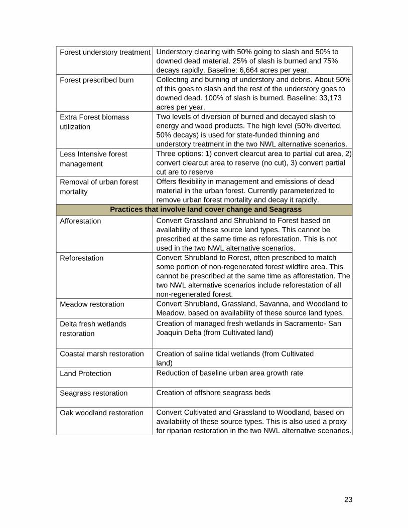
Table 3. Management Practices Currently Implemented in CALAND version 3 and relationships to the Natural and Working Lands (NWL) Scenarios. (See Section 4 for scenario descriptions and Appendices for detailed parameter values.)

Management Practice

Description/ Parameters

Practices that change ecosystem carbon exchange rate

Cultivated land soil

conservation

This is a proxy defined by a range of associated carbon

fluxes that encompasses a wide variety of potential

practices. This range is based on studies of cover crops and

conservation tillage, and compared with biogeochemical

modeling of other relevant practices. The desired extent of

NWL implementation for these practices is not included in

CALAND because it is modeled separately.

Rangeland compost

amendment

10-year or 30-year repeat compost amendment

for Grassland, Savanna, or Woodland

The 30-year repeat treatment on Grassland is used for the

two NWL alternative scenarios, but the desired extent of

NWL implementation for these practices is not included in

CALAND because it is modeled separately.

Urban forest expansion Increase forest fraction of Developed area

Practices that change ecosystem carbon exchange rate and also explicitly

transfer carbon among pools and can contribute to emissions

Forest clearcut Harvest of 66% of live and dead standing trees for

wood products and bioenergy. 25% of slash is burned and

75% decays rapidly. Baseline: 36,884 acres per year.

Forest partial cut Thinning of 20% of live and dead standing trees

for wood products and bioenergy. 25% of slash is burned

and 75% decays rapidly. Baseline: 114,833 acres per year.

Forest thinning Clearing of ladder fuels and debris through thinning – includes removal of 20% of live and dead standing trees for wood products and

bioenergy. 25% of slash is burned and 75% decays rapidly.

Baseline: 164,884 acres per year.

Forest understory treatment Understory clearing with 50% going to slash and 50% to

downed dead material. 25% of slash is burned and 75%

decays rapidly. Baseline: 6,664 acres per year.

Forest prescribed burn Collecting and burning of understory and debris. About 50%

of this goes to slash and the rest of the understory goes to

downed dead. 100% of slash is burned. Baseline: 33,173

acres per year.

Forest thinning Clearing of ladder fuels and debris through thinning – includes removal of 20% of live and dead standing trees for wood products and

bioenergy. 25% of slash is burned and 75% decays rapidly.

Baseline: 164,884 acres per year.

23

Forest understory treatment Understory clearing with 50% going to slash and 50% to

downed dead material. 25% of slash is burned and 75%

decays rapidly. Baseline: 6,664 acres per year.

Forest prescribed burn Collecting and burning of understory and debris. About 50%

of this goes to slash and the rest of the understory goes to

downed dead. 100% of slash is burned. Baseline: 33,173

acres per year.

Extra Forest biomass

utilization

Two levels of diversion of burned and decayed slash to

energy and wood products. The high level (50% diverted,

50% decays) is used for state-funded thinning and

understory treatment in the two NWL alternative scenarios.

Less Intensive forest

management

Three options: 1) convert clearcut area to partial cut area, 2)

convert clearcut area to reserve (no cut), 3) convert partial

cut are to reserve

Removal of urban forest

mortality

Offers flexibility in management and emissions of dead

material in the urban forest. Currently parameterized to

remove urban forest mortality and decay it rapidly.

Practices that involve land cover change and Seagrass

Afforestation Convert Grassland and Shrubland to Forest based on

availability of these source land types. This cannot be

prescribed at the same time as reforestation. This is not

used in the two NWL alternative scenarios.

Reforestation Convert Shrubland to Rorest, often prescribed to match

some portion of non-regenerated forest wildfire area. This

cannot be prescribed at the same time as afforestation. The

two NWL alternative scenarios include reforestation of all

non-regenerated forest.

Meadow restoration Convert Shrubland, Grassland, Savanna, and Woodland to

Meadow, based on availability of these source land types.

Delta fresh wetlands

restoration

Creation of managed fresh wetlands in Sacramento- San

Joaquin Delta (from Cultivated land)

Coastal marsh restoration Creation of saline tidal wetlands (from Cultivated

land)

Land Protection Reduction of baseline urban area growth rate

Seagrass restoration Creation of offshore seagrass beds

Oak woodland restoration Convert Cultivated and Grassland to Woodland, based on

availability of these source types. This is also used a proxy

for riparian restoration in the two NWL alternative scenarios.

24

2.2.5. Forest management

Forest management is defined here as activities with the primary goal of manipulating forest biomass without changing the long-term land type (regeneration is assumed21).

Forest management activities modeled in CALAND include a set of treatments applied to Forest (Clearcut, Partial Cut, Thinning, Understory Treatment, Prescribed Burn) and a

corresponding set with two available levels of additional slash utilization (Clearcut Slash Utilization, Partial Cut Slash Utilization, Thinning Slash Utilization, Understory

Treatment Slash Utilization, and Prescribed Burn Slash Utilization). Harvest and fuel

reduction practices result in varying amounts of carbon lost from understory, downed dead, litter, and uncollected harvest residue. These carbon losses are collected into a temporary

slash pool that is cleared each year via storage in wood products or losses to the atmosphere from bioenergy, decay, or controlled burning. Detailed descriptions of parameters are in

Appendices E, F1, and F2.

Reforestation (from Shrubland) and Afforestation (from Shrubland and Grassland) are

implemented as a land type conversion, and only one or the other can be prescribed in the

same simulation. Reforestation complements the optional non-regeneration of forest due

to wildfire22 (section 2.3.4), and can also include removal of slash for bioenergy and wood

products. These parameters are the same ones as defined in Appendices F1 and F2.

21 As detailed in the following footnote, regeneration is prevalent for these activities, and in the

case of commercial harvest reforestation is mandated, and thus it is reasonable to assume that

these activities do not change the land type. 22 There are limited data available to specifically implement reforestation and non-regeneration in

a landscape carbon model, and it is unclear whether reforestation practices significantly affect

medium- to long-term landscape level carbon exchange in comparison with natural

regeneration. Implicit forest regeneration is a reasonable assumption for forest management

practices, as there are mandates and incentives to ensure such regeneration. Additionally,

evidence suggests that natural regeneration is usually sufficient for stand replacing wildfire,

with reforestation practices primarily determining species composition. However, severe fire

and subsequent environmental conditions can affect regeneration rates of particular stands.

The unknowns include whether and how much forest area will fail to regenerate to previous

levels; how variability in regeneration success affects the long-term rate of stand or landscape

carbon accumulation; the effects of reforestation practices on the long-term rate of stand and

landscape carbon accumulation; and whether reforestation or environmental conditions

ultimately drive regeneration. Furthermore, it is unclear whether reported data lump

understory management into reforestation practices. Understory management has been shown

to increase tree carbon accumulation, but it is often applied as a post-regeneration practice. In

general, more detailed analyses of wildfire and forest regeneration data are needed to

adequately parameterize the conditions for reforestation and non-regeneration in CALAND.

The updated fire module does include optional non-regeneration with a model input argument

that determines the extent of non-regeneration within high severity burn area. Changing this

input argument allows the user to explore the uncertainty range of non-regenerated forest due

to wildfire.

25

The ten Forest management activities are parameterized based on the literature except for

the slash utilization pathways, which are aspirational targets that the CALAND user can

adjust in the carbon input file (Appendix E). All ten practices generate slash carbon, which

is either lost to the atmosphere via decay and controlled burning in the five traditional

treatments, or it can be collected and utilized in wood products or bioenergy in the five

corresponding slash utilization activities. Changes to the slash parameters can be made in

the carbon input file, but the sum of these slash fractions (Slash2Energy, Slash2Wood,

Slash2Burn, Slash2Decay in Appendices F1 and F2) must add up to equal 1.

The carbon transfer parameters for each practice are the same across regions and

ownerships. Clearcut and Partial Cut capture the average characteristics of commercial

timber harvest practices in California, with Clearcut representing practices such as

clearcutting and leaving seed trees, and Partial Cut representing practices such as selective

tree harvest and commercial thinning (Stewart and Nakamura, 2012). The most common

practice for fuel reduction is Thinning, so currently Thinning is parameterized identically

to Partial Cut. Prescribed Burn and Understory Treatment are also fuel reduction activities

with unique parameterizations due to unique sources and sinks for biomass carbon. The

wood products carbon pool is tracked using the IPCC Tier 2 guidelines (IPCC, 2006a;

equation 12.1) for estimating the next year’s wood carbon stock from the current year’s

stock, the current year’s addition, and the half-life of the wood products (52 years; Stewart

and Nakamura, 2012). Wood product carbon emissions are assumed to occur in landfills,

and are split between CO2 and CH4 following IPCC Tier 2 methods (IPCC, 2006b; section

3.1) and using CARB default values (ARB, 2016; Section IV, eq 89). The values for the

amount of harvested and slash-utilized carbon going to energy are aspirational both in

terms of the amount of traditional slash (branches, tree-tops, bark) removed from the forest

(only 4% of total harvested material is left in the forest) and the disposition of sawmill

waste. Stewart and Nakamura (2012) report 32% of harvested biomass could go to energy

for Clearcut and 75% for Partial Cut, while an average USFS estimate is 53% (McIver et

al., 2015). The proportions of slash utilization going to different end uses, and the

emissions profiles of those end uses (e.g., energy production and emission control

technologies used at bioenergy facilities) are expected to be critical to the net carbon

emissions of Forest management and will continue to be investigated.

Forest management practices affect vegetation carbon accumulation and mortality rates

(Appendix E) for a 20-year post-management period. Vegetation carbon accumulation

increases on managed land, while mortality rate can increase or decrease. These effects

vary by region and ownership and are derived from USFS FIA data (Christensen et al.,

2017). These long-term effects are implemented by applying adjustments to cumulative

managed area over the previous 20 years. To effectively emulate repeat treatments on the

same land, repeat prescriptions must occur at least 20 years apart, otherwise they will affect

carbon and mortality as if additional area has been treated. The cumulative managed area

affected during the 20-year benefit period does not necessarily equal the total cumulative

managed area because Prescribed Burn is assumed to occur on land that has undergone

Thinning or Understory Treatment within the previous 20 years. In other words, Prescribed

26

Burn area does not contribute to the cumulative managed area that experiences carbon and

mortality adjustments because the Prescribed Burn area has already been included due to

previous management. This allows Prescribed Burn to be repeated at any interval without

artificially inflating the effects of management on carbon and mortality. Conversely,

cumulative Prescribed Burn area replaces cumulative Thinning and Understory Treatment

area when adjusting fire severity because Prescribed Burn is assumed to have taken place

more recently on that particular land (see section 2.3.4).

The carbon emissions species (CO2, CH4, and BC) directly associated with each Forest

management activity are specific to the three potential pathways of carbon transfer from

land to atmosphere (controlled burn, bioenergy, and decay). All of these emissions occur within the model year and it is assumed that all carbon going to energy is burned for

electricity. The non-energy burned carbon emissions (i.e., prescribed burns and slash burning) are partitioned into CO2, CH4, and BC (i.e., 0.9952, 0.0021, and 0.0027,

respectively) based on reported emissions fractions from burned biomass and the BC

fraction of emission species (Jenkins et al., 1996), which are fixed parameters within the model. The burned carbon emissions from energy are currently partitioned into CO2, CH4,

and BC (i.e., 0.9994, 0.0001, and 0.0005, respectively) based on average emissions

fractions for California boiler plants (Carreras-Sospedra et al., 2015) and the same BC fractions of species as for non-energy (which gives different BC emissions from energy

because the species profile is different from non-energy). Other efforts are underway to

examine potential emissions data from nascent bioenergy technologies, including those funded through the California Energy Commission’s Electric Program Investment Charge

(EPIC) Program, based on CALAND feedstock production estimates. Total annual non-burned carbon emissions are released as CO2 within the model year as a result of decay of

removed biomass or wood products.

2.2.6. Wildfire

Spatially explicit wildfire area

Annual wildfire area is simulated in each Forest, Woodland, Savanna, Shrubland, and

Grassland land category under one of three possible climates (historical, RCP 4.5, and

RCP 8.5). The user chooses the wildfire option when creating the scenario input file using

write_caland_inputs.r. The historical option is a constant, historical annual burn area,

while the climate change options (RCP 4.5 and RCP 8.5) are projected-climate annual burn

areas (see section 2.3.5 for climate description). The climate change data are derived from

1/16-degree gridded burn area estimates generated for the California Fourth Climate

Change Assessment23 (Westerling, 2018). Specifically, they are the burn area data for the

“average” climate model (CanESM2) and central population scenario.

23 These data are available at: http://cal-adapt.org/data/wildfire/; a corresponding viewer is

available at: http://cal-adapt.org/tools/wildfire/.

27

The gridded burn area values were distributed to CALAND region-ownerships, and within

each region-ownership (the boundaries of which do not change over time) the burn area

was distributed proportionally to Forest, Woodland, Savanna, Shrubland, and Grassland

land types (the areas of which do change over time). These land types were selected

through visual overlay of the CAL FIRE fire perimeters data24 with the land cover type

data. The initial 2010 wildfire area for the climate change options is calculated as the 2001-

2015 modeled average of the respective climate scenario. For the historical climate run the

constant annual value is the RCP 8.5 initial area (185,237 ha statewide). Note that the RCP

4.5 initial area is similar (195,095 ha statewide), but that both of these are lower than the

non-spatial statewide area used in CALAND v2 (243,931 ha statewide, 2001-2015

average). There is sufficient flexibility in the current scenario input file to prescribe a

variety of fire cases, given the appropriate data.

Wildfire severity and non-regeneration

Wildfire severity is defined as the fraction of total burn area assigned to high, medium,

and low severity burns, with corresponding amounts of carbon burned or transferred to

dead biomass pools. The initial values and annual increase of high severity fraction are

based on samples of CA fires from 1984 to 2006 (Miller et al., 2009 and Miller et al.,

2012) (Table 4). The user can specify either full regeneration or a threshold distance from

burn edge beyond which a high severity patch will not regenerate (Collins et al., 2017) and

will be converted to Shrubland. Non-regeneration is the default, with a threshold of 120m,

which has been used to study California wildfire because it is the likely limit of California

conifer seed dispersal (Collins et al., 2017, Stevens et al., 2017). A shorter distance

increases non-regenerated area, and a longer distance decreases non-regenerated area.

Forest management for reduction of high severity wildfire

Forest management reduces the high severity fraction on managed land for a period of 20

years (equal to the carbon accumulation benefit period for forest management). These

reductions are specified for three categories of fuel reduction treatments (Lyderson et al.,

2013) (Table 4). As prescribed burn is assumed to occur on land that has been managed

within the previous benefit period (20 years), it replaces the severity benefits of thinning

and understory treatment. In other words, the cumulative prescribed burn area replaces the

same area of thinning and understory treatment when calculating burn severity reduction.

The area to which these adjustments are applied is calculated using the fraction of forest

area burned multiplied by the fraction of forest area managed in order to maintain random

spatial distributions of both processes within a land category.

24 CAL FIRE FRAP Date, Fire Perimeters, available online:

http://frap.fire.ca.gov/data/statewide/FGDC_metadata/fire15_1_metadata.xml

28

Wildfire carbon dynamics

Wildfire carbon emissions are separated into an immediately burned pathway and a rapid decay pathway for wildfire-killed, non-burned biomass (Pearson et al., 2009). All burned wildfire carbon emissions are partitioned into CO2, CH4, and BC (i.e., 0.9952, 0.0021, and 0.0027, respectively) based on the same reported non-energy burned carbon emissions fractions (Jenkins et al., 1996) used for Forest management. The rapid decay pathway for wildfire-killed biomass assumes a fractional 0.09 per year decomposition rate based on recommended decay rates for non-solid-log material (Harmon et al., 1987). The corresponding CO2 emissions result in 59% of wildfire-killed biomass decaying within 10 years of the fire, and 90% of fire-killed biomass decaying within 25 years.

Table 4. Management Effects on Wildfire Severity Wildfire severity percent of total burn area and percent decreases/increases (negative/positive) in severity percent due to fuel reduction management. The initial high severity percent is increased annually by 0.27%, with proportional decreases in medium and low severity fractions. The management adjustments are the percent change in the annual value of the respective severity class.

Wildfire Severity

Initial value Management Effects on Wildfire

Severity

Prescribed

burn Thinning, Partial cut,

and Clearcut Understory treatment

High 26% -68% -26% -24%

Medium 29% -13% +10% +30%

Low 45% +94% +19% -6%

2.3.7. Land type conversion

Land type conversion is driven by three main levers in CALAND. First, there are baseline

annual area changes that are applied to all land categories except for Water and Ice, which

are assumed to remain constant. Second, several management practices effect land type

conversion, including avoided conversion (Growth reduction), all the restoration practices,

forest area expansion (Afforestion), and Reforestation (complementary to wildfire non-

regeneration) (see 2.3.4). Third, wildfire constrains land type conversion through optional

non-regeneration (conversion to Shrubland) of some Forest area burned by high severity

wildfire (see 2.3.6).

Baseline annual area change inputs: options and methods of derivation

There are two options for baseline annual area change inputs: remote sensing-based

extrapolation, representing historical trends, and model-based extrapolation, representing

land-use driven trends of urban expansion and expansion/contraction of cultivated lands.

One of these options is designated when creating the input files using write_caland.r.

29

The remote sensing-based option is derived from LANDFIRE remote sensing data, and it

is based on the difference in land cover between 2001 and 2010 with adjustments for slight

differences in total area between years.25 To calculate changes in area for each land

category, the LANDFIRE raster datasets for 2001 and 2010 had to be spatially aligned

with CALAND’s geographic projection system and resolution of 30 m2. Then the two

LANDFIRE landtype maps consisting of 158 and 204 land types in 2001 and 2010,

respectively, were aggregated into CALAND’s 15 land types (see section 2.1.1). The 15

land types were then intersected with CALAND’s 9 ownership classes and 9 regional

boundaries to define the spatial boundaries and areas of CALAND’s 940 land categories.

Lastly, the differences in total area for each land category were calculated.

The land-use driven modeling option is based on the business-as-usual projections of

annual land cover changes in urban and cultivated lands from the Land Use and Carbon

Scenario Simulator (LUCAS) of Sleeter et al. (2017). LUCAS simulates annual area

changes of 11 discrete land cover categories, however only changes in Urban Area and

Cultivated Land26 areas were used. The reason for this is two-fold; first, the main drivers

of land cover change in LUCAS are urban expansion and expansion/contraction of

cultivated lands. Second, there are several land types in CALAND that are not represented

in LUCAS. Thus, all other land type areas in each corresponding region-ownership

combination, excluding water and ice, increase or decrease in proportion to their relative

areas to offset the net change in urban and cultivated area, ensuring that area is conserved.

A total of 92 years (2010-2101) of annual area changes were calculated at the 30 m2

resolution using the LUCAS outputs, from which a single average annual area change was

calculated for each CALAND land category.

Implementation of baseline area changes

At the end of each model year the selected annual area changes are applied to the current

land cover (Sections 2 and 2.1.1). The conversion areas are calculated independently for

each ownership class within each region. The annual changes are first adjusted to account

for land availability and to ensure that restored land type area persists. Conversion matrices

are then calculated for each region-ownership combination to determine the areas of each

land type being converted to (and from) another land type. These transition values are

calculated by splitting individual land type gains proportionally across all available land

type losses.

25 For example, USFS Coastal Marsh is zero in 2010, but also shows a loss because it is 0.09 ha

in 2001. Such losses are set to zero and redistributed among the other land types to ensure a

net total area change of zero. 26 Annual and perennial agriculture areas from LUCAS outputs were combined into a single

cultivated land type to calculate annual area changes in order to correspond to the single

cultivated land type in CALAND

30

Permanence and uncertainty of baseline annual area change options

In contrast to the land-use driven option, which only captures land type conversions caused

by urban expansion and cultivated expansion/contraction, the remote sensing option

captures all land type conversions (including those not driven by human activity). The

land-use driven option may better capture Urban and Cultivated land cover change

dynamics, but it does not capture potential land cover change due to non-anthropogenic

disturbances, including permanent change due to severe disturbances, such as fire. On the

other hand, the remote sensing option lacks information about the permanence of all land

type changes due to having only two years for comparison. For example, a forest fire or

clear cut harvest may show up in the remote sensing data as Forest in one year and

Grassland in another, but we do not know the cause of this change or if the land cover

change is permanent. Forest regeneration periods can be long and there is evidence that

some severely burned areas do not regenerate. Thus, CALAND’s default assumptions

include regeneration after Forest management and permanent land type conversion due to

baseline trends, with optional non-regeneration of specified portions of high-severity

wildfire patches (Section 2.3.4).

The land cover change inputs are highly uncertain, based on the large differences between

the two options and this uncertainty is not quantified. Sources of this uncertainty include

non-permanence, misclassification, and crosswalk uncertainty (due to the combination of

two different classification schemes). For example, in the remote-sensing based change

data, annual Grassland expansion and Shrubland contraction are an order of magnitude

larger than the other land type changes, with the loss of shrub biomass contributing

significantly to a net California landscape carbon source in our baseline projections (not

only in CALAND projections, but likely for the ARB Inventory estimate as well). This

apparent Shrubland to Grassland conversion may actually represent large area shrub fires

that occurred within a few years prior to 2010 and had not yet regenerated, giving the false

impression that huge amounts of Shrubland were permanently converted to Grassland as

part of a decadal trend. Furthermore, Water and Ice expansion could be due to unique

weather patterns in 2001 and 2010 and/or different dates of the imagery used for each year.

While there is always some misclassification error in remote sensing products, particular

problems in distinguishing between orchards/vineyards (Cultivated Land) and vegetation

in developed areas (Urban Area; i.e., parks, yards, street trees, etc.) have been found.

Combining this misclassification with uncertainty introduced by combining two different

classification schemes into one (crosswalk uncertainty) provides some explanation of why

the remote-sensing based data estimate expansion of Cultivated Land (which is small

relative to other land type changes), in contrast to other analyses showing similar amounts

of Cultivated Land contraction. Additionally, the remote-sensing based data may be

capturing some land clearing and cultivation occurring outside the scope of the other

analyses.

Due to these issues, the land-use based data are the default land cover change inputs. This

approach may better capture Urban Area and Cultivated Land cover change dynamics, but

31

may miss potential land cover change due to non-anthropogenic sources, including

permanent change due to severe disturbances, such as wildfire. A more complete approach

would include a time-series remote sensing analysis of all land cover types and additional

disturbance information.

Nonetheless, uncertainty in absolute carbon projection of the mean state in CALAND is

significantly affected by uncertainty in land cover change, which is one reason why

CALAND currently should be used only to examine differences between alternative

scenarios and the business-as-usual scenario.

Management practice effects on land type conversion

The management practices that modify land type conversion in CALAND include

Restoration (Meadow, Coastal Marsh, Fresh Marsh, Seagrass), avoided conversion

(labeled as Growth, which reduces the growth rate of Urban Area), Afforestation and

Reforestation. Avoided conversion is prescribed and implemented as an annually

decreasing Urban growth rate. The reduction is applied to the baseline annual area growth

rates for Urban Areas, which consequently reduces the loss of other land types. When

using the remote sensing option for baseline annual area change, the Urban Area growth

reduction will also increase the expansion of other growing land type areas. After avoided

conversion is applied, prescribed annual Restoration targets are fulfilled to the extent that

land types areas are available. Coastal Marsh and Fresh Marsh are restored only from

Cultivated Land. This land conversion aligns with current practices (Steve Deverel,

personal communication), although Coastal Marsh can also be restored from seasonal

wetlands and open water. Meadow is restored proportionally from existing Shrubland,

Grassland, Savanna, and Woodland. Seagrass is restored from anything else in the ocean

(i.e., non-Seagrass is not tracked). Afforestation proportionally converts Shrubland and

Grassland to Forest and Reforestation converts Shrubland to Forest. All restored areas

persist throughout the simulation period.

Land conversion effects on ecosystem carbon dynamics

There are two main modes in which land type conversion affects carbon dynamics in

CALAND. First, changes in the area trajectory of each land category relative to the

baseline scenario will result in compounding carbon impacts (cost or benefit) based on the

net difference in carbon dynamics of the new area distribution of land categories. Not only

can annual carbon exchange rates differ across the landscape with a new distribution of

land category areas, but there can be new interactions with climate, wildfire,

(non)regeneration, and subsequent management. The second and most immediate impact

of land conversion on carbon dynamics is the change in existing carbon stocks that occurs

the same year as the converting land types.

The initial changes in existing carbon stocks are based on differences in carbon density

between the exchanging land types, with the exception of land conversion to Urban Area

or Cultivated Land. For these exceptions, carbon transfer parameters from the academic

literature are used instead (see Appendix E for parameters). In all other cases, if

aboveground carbon in the new land type is greater than in the old land type, all the carbon

32

from the old land type is transferred to the new land type based on the assumption that it

takes time for the converted land to gain enough carbon to match the average carbon

density of the new land type. Conversely, if the new land type has less aboveground carbon

than the old land type, the difference is emitted to the atmosphere within the year and only

the remaining portion is transferred to the new land type. This assumes that carbon loss is

immediate upon conversion, which is often the case for this type of transition, but can

depend on how the conversion occurred. For belowground carbon (roots and soil), it is

assumed that soil and root carbon losses are dictated by belowground carbon dynamics

rather than the conversion. Thus, all belowground carbon is transferred from the old land

type to the new land type (i.e., no carbon loss). Seagrass expansion initially dilutes carbon

density because there is no initial gain in carbon due to unknown conditions of the new

area. Seagrass contraction does not lose carbon to the atmosphere because it is assumed

that the carbon is trapped in the ocean floor (carbon density does not change). All carbon

losses corresponding with conversion to land types other than Urban Area and Cultivated

Land occur as CO2 emissions to the atmosphere.

Conversion to Urban Area or Cultivated Land is a special case because substantial

alteration of the landscape is required. The carbon transfer parameter values for conversion

to Urban Area and Cultivated Land are identical (see Appendix E for parameters). If the old land type is Forest, the conversion involves a timber harvest that is currently

parameterized as a Clearcut with 100% of the biomass removed. This means that only live main canopy and standing dead are available for wood products and bioenergy, and that

all uncollected harvest residue and other vegetation carbon (understory, down dead, and litter) is currently assumed to decay to the atmosphere as CO2. However, the new slash

biomass utilization pathways are also available for this type of land conversion.

Partitioning of the carbon emissions into CO2, CH4, and BC follows the same methods as

described above for Forest management (section 2.3.3).

Otherwise, all biomass carbon (above, dead, and roots) and a fraction of the soil carbon

are removed and decay to the atmosphere within one year as CO2. The fraction of soil

carbon lost to the atmosphere is based on a comprehensive review of adjacent-plot studies for agriculture, which shows that most of the soil carbon loss occurs within the first three

years of conversion (Davidson and Ackerson, 1993).

3. Model outputs and diagnostics Each output table in the output file provides annual values for a single variable (Appendix

G), by land category, with additional records for aggregated regions and/or land types.

Change values, which are the differences between the final and initial year values, are also

included in these tables. There are seven main categories of output table, including area,

carbon stock, carbon density, land-atmosphere carbon exchange, wood products, GHG

species partitioning, and CO2-equivalent emissions. Land category area, carbon stock,

carbon density, and cumulative gain/loss variables represent (up to) the beginning of the

labeled year, while managed and burned areas and annual gain/loss variables represent

activities or fluxes during the labeled year. The output records are labeled with the

identification number corresponding to the land category raster map so that values can be

displayed by land category using a Geographic Information System.

33

There is a primary diagnostic function (defined in plot_caland.r) that plots several

variables (see appendix G for variables) from the model output file, and two secondary

diagnostic functions (defined in plot_scen_types.r and plot_uncertainty.r?) that use files

generated by the plot_caland function. Plot_caland compares one or more scenarios with

a baseline scenario, and has two modes: 1) general diagnostics and 2) individual practice

evaluation. The general diagnostics mode produces a variety of time series and snapshot

plots for regular scenario simulations, while the individual practice mode is designed to

calculate per-area statistics for a single practice from a pair of simulations carefully

constructed to isolate the desired practice. Plot_caland supports CALAND outputs with

and without black carbon, plots for aggregate and individual land categories, a cutoff year

for time series, and a selection for acres or hectares as the diagnostic area units.

The secondary diagnostic functions allow a user to generate some tailored figures for

specified variables, scenarios, and land categories (with optional aggregation of all

regions/ownerships/land types). Plot_scen_types co-plots multiple land types within a

single scenario, and plot_uncertainty generates shaded uncertainty plots from a set of three

appropriate simulations (e.g., mean, maximum, and minimum emission configurations).

4. Baseline and alternative land use and management scenarios for the Natural and Working Lands Climate Change Implementation Plan

The California Natural and Working Lands Climate Change Implementation plan focuses on the carbon consequences of state interventions to land management. The three associated scenarios (a baseline and two alternatives) can be run using historical (no climate effects), RCP4.5, and RCP8.5 climate effects on ecosystem fluxes (2.3.5) and wildfire areas (2.3.4). The baseline scenario includes ecosystem carbon fluxes, wildfire area, historical forest harvest areas for even-age and uneven-age management on private land, historical USFS-funded fuel reduction areas on USFS and private land (Table 3), a constant urban forest fraction of 15% (McPherson et al., 2017), and historical land use and cover change based on Sleeter et al. (2018) (see section 2.3.6). Additionally, mortality in urban forest is removed from the system and decays to the atmosphere, and forest tree mortality is doubled from 2015-202527 to emulate the observed impacts of insects and drought that are not captured by the data used to initialize and parameterize the model.28

27 On a biomass/carbon basis. Recently published tree mortality numbers indicate that the annual

average number of trees that died in 2015-2016 is about 20 times the 2010-2014 annual

average. Tree Mortality Task Force, Tree Mortality Facts and Figures (April 2017) Available

online:

http://www.fire.ca.gov/treetaskforce/downloads/TMTFMaterials/Facts_and_Figures_April_2

01 7.pdf. Accessed Aug. 15, 2017. 28 The primary effect of increasing mortality in CALAND is carbon transfer from live to dead

pool.

34

The forest harvest rates are derived from Robards and Nickerson (2013) and the forest fuel reduction rates are derived from the CAL FIRE Draft Vegetation Treatment Program Environmental Impact report (VTPEIR) (2004-2013; CAL FIRE, 2016) and the USFS Pacific Southwest Region office (2008-2015; PSR, Jason Ko, personal communication). These USFS-funded fuel reduction areas are the same for the baseline and alternative scenarios because they are outside the scope of state-funded intervention. No state-funded forest management activities are included in the baseline scenario.

The two alternative scenarios each consist of the addition of a suite of activities (Table 3)

for land use (e.g., conservation/avoided conversion), land management (e.g., fuel

reduction), and restoration (e.g., fresh marsh) to the baseline scenario. Each activity is

applied annually to the appropriate land type(s) at a given extent (i.e., acreage) over the

2019-2030 timeframe. After 2030 the management practices return to baseline with three

exceptions: 1) the resulting growth rate for 2030 is held constant, 2) urban forest fraction

continues to expand at the same rate as in previous years, and 3) state-funded forest fuel

reduction practices repeat every 20 years for maintenance (i.e., the 12-year block starts

again in 2039). These scenarios have been developed cooperatively by many state agencies

and represent goals for California land management, excluding expectations for the

Healthy Soils program, which are simulated separately by another model. The primary

difference between the two alternative scenarios is the area of implementation of the

various practices. For example, Alternative A has a 50% reduction in urban growth rate

by 2030, while Alternative B has a 75% reduction by 2030. Full details of the alternative

scenarios are reported in the Natural and Working Lands Implementation Plan.

The two alternative scenarios have been compared with the baseline to estimate the effects

of different land management suites on California’s landscape carbon budget (Figure 3).

Uncertainty of these estimates is based only on uncertainties in land carbon flux values

and initial carbon densities. The uncertainty envelope is defined by a low emission

configuration (high land carbon uptake rates and low initial carbon densities) and a high

emission configuration (low land carbon uptake rates and high initial carbon densities).

While less intensive forest management reduces carbon emissions, increased forest fuel

reduction dramatically increases carbon emissions. Longer-term benefits of forest and

restoration practices, combined with temporal gaps in forest fuel reduction

implementation, eventually compensate for early fuel reduction emissions to provide

cumulative reductions in landscape carbon emissions after a scenario-dependent time

period.

35

Figure 3. Total cumulative CO2 equivalent impacts of two Natural and Working Lands scenarios on landscape carbon emissions under RCP 8.5.

5. Looking Ahead

CALAND continues to evolve to better serve the needs of the State and other

stakeholders. In addition to minor upgrades there are four main avenues for further

development: 1) Improve land use/cover change to provide better absolute carbon budget

estimates, 2) Develop additional land/vegetation management practices for Cultivated

Land, Woodland, Savanna, Shrubland, and Grassland, 3) Integration with bioenergy

pathway tools such as those being developed in the CEC-funded California Biopower

Impacts project, and 4) Disaggregation to finer spatial scales. To pursue any one of these

main tasks will require additional resources and considerable effort.

−600

−400

−200

0

2025 2050 2075 2100

Year

Cha

nge

fro

m B

aselin

e (

MM

T C

O2e)

Scenario

A

All_region All_own All_land Scenario_Av6_default_RCP85Total_CumCO2eq_all_diff

−800

−600

−400

−200

0

2025 2050 2075 2100

Year

Ch

ange

fro

m B

aselin

e (

MM

T C

O2e)

Scenario

B

All_region All_own All_land Scenario_Bv6_default_RCP85Total_CumCO2eq_all_diff

−600

−400

−200

0

2025 2050 2075 2100

Year

Cha

nge

fro

m B

aselin

e (

MM

T C

O2e)

Scenario

A

All_region All_own All_land Scenario_Av6_default_RCP85Total_CumCO2eq_all_diff

−800

−600

−400

−200

0

2025 2050 2075 2100

Year

Cha

nge

fro

m B

aselin

e (

MM

T C

O2e)

Scenario

B

All_region All_own All_land Scenario_Bv6_default_RCP85Total_CumCO2eq_all_diff

36

Appendices

37

Appendix A: Land Categories identified for use in CALAND Variable terms used in the model are in parenthesis.

Spatial Regions

Key Terms Definition

Central Coast (Central_Coast) See Figures 1 and A1

Central Valley See Figure 1 and A1

Delta Legal Delta plus Suisun Marsh, see Figure 1

Deserts See Figures 1 and A1

Eastside See Figures 1 and A1

Klamath See Figures 1 and A1

North Coast (North_Coast) See Figures 1 and A1

Sierra Cascades (Sierra_Cascades) See Figures 1 and A1

South Coast (South_Coast) See Figures 1 and A1

Ownership Classes

Key Terms Definition

Bureau of Land Management (BLM) Bureau of Land Management

Department of Defense (DoD) Department of Defense

Easement Conservation easement, regardless of ownership, and Non-Profit Conservancies and Trusts

Local Government (Local_gov) Local government (e.g., city, county)

National Park Service (NPS) National Park Service

Other Federal Government Land (Other_fed)

Bureau of Indian Affairs, Bureau of Reclamation, US Fish and Wildlife Service, Other Federal Lands, USFS Wilderness area

Private All land under private ownership that is not in the Easement category

State Government (State_gov) CA Dept. of Fish and Wildlife, CA Dept. of Forestry and Fire Protection, CA Dept. of Parks and Recreation, Other State Lands

Non-wilderness United States Forest Service Land (USFS_nonwild)

All Forest Service land that is not designated as Wilderness area

38

Appendix A: Land Categories identified for use in CALAND Variable terms used in the model are in parenthesis.

Land Types

Key Terms Definition

Water Open water

Ice Ice, permanent snow

Barren Little to no vegetation

Sparse Sparse vegetation

Desert Desert vegetation

Shrubland Shrubs, chaparral

Grassland Grassland

Savanna Grass with sparse trees

Woodland Scattered trees with grass

Forest Trees are the dominant vegetation

Meadow Inland seasonally wet grassland

Tidal Marsh (Coastal_Marsh) Tidal marsh

Fresh Marsh (Fresh_Marsh) Restored and managed Delta wetlands

Cultivated Land (Cultivated) Annual and perennial crops, including hay and cultivated pasture

Urban Area (Developed_all) Developed land, including associated vegetation such as parks and yards

Seagrass (Ocean, Other_fed) Offshore seagrass beds

39

Figure A1: Recommended aggregation of USFS California Level 2 ecological subregions. The Delta region has been delineated primarily from the Central

Valley region.

40

Appendix B: Annual net carbon exchange in live vegetation and soil (sans mortality) under historic climate. Data are presented as mean plus and minus SD, with positive values indicating carbon uptake. Carbon losses and gains due to mortality are not included in vegetation and soil carbon exchange values, respectively, unless otherwise noted.

Land Type

Region Ownership

Net Carbon Exchange

Source Vegetation Soil

Mg C ha-1 y-1

Water All All NA1 02

Ice All All NA1 02

Barren All All 02 02

Sparse All All 02 02

Desert All All 02 0.76 ± 0.07 Hastings et al., 2005, and Wohlfahrt et al., 2008

(soil)

Shrubland All All 0.93 ± 0.313 0.28 ± 0.08 Quideau et al., 1998 (vegetation and soil)

Grassland All All 02 -2.22 ± 1.29Based on expert opinion due to lack of available data (vegetation); and Ma et al., 2007, and Ryals

and Silver, 2013 (soil)

Savanna All All 3.67 ± 0.684 -2.69 ± 0.475 Ma et al., 2007 (vegetation and soil)

Woodland All All 3.67 ± 0.684 -2.69 ± 0.475 Ma et al., 2007 (vegetation and soil)

Meadow All All 02 0.95 ± 0.25 Drexler et al., 2015 (soil)

Coastal Marsh

All All 02 1.44 ± 1.23 Callaway et al., 2012, and Chmura et al., 2003 (soil)

Fresh Marsh

All All NA1 3.37 ± 0.33 Based on expert opinion due to lack of available

data (vegetation); and Knox et al., 2015 (soil)

Cultivated Non-Delta All 02 0.19 ± 0.26 Based on expert opinion due to lack of available

data (vegetation); and Mitchell et al., 2015, Wu et al., 2008, and Kong et al., 2005 (soil)

Cultivated Delta All 02 -2.82 ± 2.51Based on expert opinion due to lack of available

data (vegetation); and Hatala et al., 2012, and Knox et al., 2015 (soil)

Urban Central Coast

All 1.45 ± 0.046 02,7 McPherson et al., 2017 (vegetation)

Urban

Central Valley

All

0.95 ± 0.0066 02,7

McPherson et al., 2017 (vegetation) Delta 0.95 ± 0.0066 02,7

Deserts 0.20 ± 0.016 02,7

Eastside 0.70 ± 0.016 02,7

41

Appendix B: Annual net carbon exchange in live vegetation and soil (sans mortality) under historic climate. Data are presented as mean plus and minus SD, with positive values indicating carbon uptake. Carbon losses and gains due to mortality are not included in vegetation and soil carbon exchange values, respectively, unless otherwise noted.

Land Type

Region Ownership

Net Carbon Exchange

Source Vegetation Soil

Mg C ha-1 y-1

Klamath 0.70 ± 0.016 02,7

North Coast

1.96 ± 0.076 02,7

Sierra Cascades

0.70 ± 0.016 02,7

Forest All Other federal 1.82 ± 0.128,9 0.71 ± 0.3010 Christensen et al., 2017, and Jenkins et al., 2003 (vegetation); Quideau et al., 1998 (soil)

Forest Central Coast

U.S. Bureau of Land Management 0.44 ± 0.268,9 0.71 ± 0.3010

Christensen et al., 2017, and Jenkins et al., 2003 (vegetation); Quideau et al., 1998 (soil)

U.S. Department of Defense 0.44 ± 0.268,9 0.71 ± 0.3010

Conservation Easement Protected 1.85 ± 0.428,9 0.71 ± 0.3010

Local Government 2.62 ± 0.828,9 0.71 ± 0.3010

National Park Service 0.44 ± 0.268,9 0.71 ± 0.3010

Private 2.03 ± 0.398,9 0.71 ± 0.3010

State Government 2.62 ± 0.828,9

0.71 ± 0.3010

USFS (non-wilderness) 0.74 ± 0.358,9 0.71 ± 0.3010

Forest Central Valley

U.S. Bureau of Land Management 02 0.71 ± 0.3010 Christensen et al., 2017, and Jenkins et al., 2003

(vegetation); Quideau et al., 1998 (soil)

Forest Central Valley

U.S. Department of Defense 02 0.71 ± 0.3010

Christensen et al., 2017, and Jenkins et al., 2003 (vegetation); Quideau et al., 1998 (soil)

Conservation Easement Protected 1.26 ± 0.808,9 0.71 ± 0.3010

Local Government 0.79 ± 0.958,9 0.71 ± 0.3010

Private 1.15 ± 0.748,9 0.71 ± 0.3010

State Government 0.79 ± 0.958,9 0.71 ± 0.3010

Forest Delta

U.S. Bureau of Land Management 0.00 ± 0.002 0.71 ± 0.3010

Christensen et al., 2017, and Jenkins et al., 2003 (vegetation); Quideau et al., 1998 (soil)

U.S. Department of Defense 02 0.71 ± 0.3010

Conservation Easement Protected 1.26 ± 0.808,9 0.71 ± 0.3010

Local Government 0.79 ± 0.958,9 0.71 ± 0.3010

Private 1.15 ± 0.748,9 0.71 ± 0.3010

State Government 0.79 ± 0.958,9 0.71 ± 0.3010

42

Appendix B: Annual net carbon exchange in live vegetation and soil (sans mortality) under historic climate. Data are presented as mean plus and minus SD, with positive values indicating carbon uptake. Carbon losses and gains due to mortality are not included in vegetation and soil carbon exchange values, respectively, unless otherwise noted.

Land Type

Region Ownership

Net Carbon Exchange

Source Vegetation Soil

Mg C ha-1 y-1

Forest Deserts

U.S. Bureau of Land Management 0.05 ± 0.038,9 0.71 ± 0.3010

Christensen et al., 2017, and Jenkins et al., 2003 (vegetation); Quideau et al., 1998 (soil)

U.S. Department of Defense 0.05 ± 0.038,9 0.71 ± 0.3010

Conservation Easement Protected 0.32 ± 0.148,9 0.71 ± 0.3010

Local Government 0.41 ± 0.358,9 0.71 ± 0.3010

National Park Service 0.05 ± 0.038,9 0.71 ± 0.3010

Private 0.27 ± 0.118,9 0.71 ± 0.3010

State Government 0.41 ± 0.358,9 0.71 ± 0.3010

USFS (non-wilderness) 0.65 ± 0.158,9 0.71 ± 0.3010

Forest Eastside

U.S. Bureau of Land Management 0.20 ± 0.058,9 0.71 ± 0.3010

Christensen et al., 2017, and Jenkins et al., 2003 (vegetation); Quideau et al., 1998 (soil)

U.S. Department of Defense 0.20 ± 0.058,9 0.71 ± 0.3010

Conservation Easement Protected 0.50 ± 0.218,9 0.71 ± 0.3010

Local Government 1.32 ± 1.528,9 0.71 ± 0.3010

National Park Service 0.20 ± 0.058,9 0.71 ± 0.3010

Private 1.21 ± 0.308,9 0.71 ± 0.3010

Forest Eastside State Government 1.32 ± 1.528,9 0.71 ± 0.3010 Christensen et al., 2017, and Jenkins et al., 2003

(vegetation); Quideau et al., 1998 (soil) USFS (non-wilderness) 0.74 ± 0.118,9 0.71 ± 0.3010

Forest Klamath

U.S. Bureau of Land Management 3.00 ± 0.858,9 0.71 ± 0.3010 Christensen et al., 2017, and Jenkins et al., 2003

(vegetation); Quideau et al., 1998 (soil) U.S. Department of Defense 3.00 ± 0.858,9 0.71 ± 0.3010

Forest Klamath

Conservation Easement Protected 2.38 ± 0.308,9 0.71 ± 0.3010

Christensen et al., 2017, and Jenkins et al., 2003 (vegetation); Quideau et al., 1998 (soil)

Local Government 1.36 ± 0.798,9 0.71 ± 0.3010

National Park Service 3.00 ± 0.858,9 0.71 ± 0.3010

Private 2.74 ± 0.248,9 0.71 ± 0.3010

State Government 1.36 ± 0.798,9 0.71 ± 0.3010

USFS (non-wilderness) 2.61 ± 0.178,9 0.71 ± 0.3010

Forest North Coast

U.S. Bureau of Land Management 5.18 ± 1.888,9 0.71 ± 0.3010 Christensen et al., 2017, and Jenkins et al., 2003

(vegetation); Quideau et al., 1998 (soil) U.S. Department of Defense 5.18 ± 1.888,9 0.71 ± 0.3010

Conservation Easement Protected 4.11 ± 0.628,9 0.71 ± 0.3010

43

Appendix B: Annual net carbon exchange in live vegetation and soil (sans mortality) under historic climate. Data are presented as mean plus and minus SD, with positive values indicating carbon uptake. Carbon losses and gains due to mortality are not included in vegetation and soil carbon exchange values, respectively, unless otherwise noted.

Land Type

Region Ownership

Net Carbon Exchange

Source Vegetation Soil

Mg C ha-1 y-1

Local Government 5.98 ± 1.538,9 0.71 ± 0.3010

National Park Service 5.18 ± 1.888,9 0.71 ± 0.3010

Private 4.91 ± 0.458,9 0.71 ± 0.3010

State Government 5.98 ± 1.538,9 0.71 ± 0.3010

USFS (non-wilderness) 7.94 ± 5.158,9 0.71 ± 0.3010

Forest Sierra

Cascades

U.S. Bureau of Land Management 1.48 ± 0.188,9 0.71 ± 0.3010

Christensen et al., 2017, and Jenkins et al., 2003 (vegetation); Quideau et al., 1998 (soil)

U.S. Department of Defense 1.48 ± 0.188,9 0.71 ± 0.3010

Conservation Easement Protected 1.20 ± 0.128,9 0.71 ± 0.3010

Local Government 2.55 ± 0.828,9 0.71 ± 0.3010

National Park Service 1.48 ± 0.188,9 0.71 ± 0.3010

Private 2.09 ± 0.148,9 0.71 ± 0.3010

State Government 2.55 ± 0.828,9 0.71 ± 0.3010

Forest Sierra

Cascades USFS (non-wilderness) 2.45 ± 0.118,9 0.71 ± 0.3010

Christensen et al., 2017, and Jenkins et al., 2003 (vegetation); Quideau et al., 1998 (soil)

Forest South Coast

U.S. Bureau of Land Management 0.05 ± 0.038,9 0.71 ± 0.3010 Christensen et al., 2017, and Jenkins et al., 2003

(vegetation); Quideau et al., 1998 (soil)

Forest South Coast

U.S. Department of Defense 0.05 ± 0.038,9 0.71 ± 0.3010

Christensen et al., 2017, and Jenkins et al., 2003 (vegetation); Quideau et al., 1998 (soil)

Conservation Easement Protected 0.32 ± 0.148,9 0.71 ± 0.3010

Local Government 0.41 ± 0.358,9 0.71 ± 0.3010

National Park Service 0.05 ± 0.038,9 0.71 ± 0.3010

Private 0.27 ± 0.118,9 0.71 ± 0.3010

State Government 0.41 ± 0.358,9 0.71 ± 0.3010

USFS (non-wilderness) 0.65 ± 0.158,9 0.71 ± 0.3010

Seagrass Ocean Other Federal NA1 0.45 ± 0.45 Mcleod et al., 2011 (soil) 1 Carbon pool is not represented in CALAND. 2 Due to lack of data, static carbon density is assumed (i.e., net carbon exchange is 0 Mg C ha-1 y-1) based on expert opinion. 3 Only includes aboveground main canopy net carbon exchange; belowground main canopy and understory carbon exchange are additional and are calculated

annualyannually as follows:

44

(a) 𝑪𝑶𝟐 𝒓𝒐𝒐𝒕 = 𝒇𝒓𝒐𝒐𝒕

𝒇𝒔𝒕𝒆𝒎∙ 𝑪𝑶𝟐 𝒔𝒕𝒆𝒎, where 𝑪𝑶𝟐 𝒓𝒐𝒐𝒕 is the C accumulation in the root (Mg C ha-1 y-1), 𝑪𝑶𝟐 𝒔𝒕𝒆𝒎 is the CO2 uptake in the stem (bole) (Mg C ha-1 y-1), 𝒇𝒓𝒐𝒐𝒕 is the

ratio of root to aboveground main canopy carbon density (fraction), and 𝒇𝒔𝒕𝒆𝒎 is the constant fraction (0.66) of stem to aboveground main canopy.

(b) 𝑪𝑶𝟐 𝒖𝒏𝒅𝒆𝒓𝒔𝒕𝒐𝒓𝒚 = 𝒇𝒖𝒏𝒅𝒆𝒓𝒔𝒕𝒐𝒓𝒚 ∙ 𝑪𝑶𝟐 𝒂𝒃𝒐𝒗𝒆 𝒎𝒂𝒊𝒏 , where 𝑪𝑶𝟐 𝒖𝒏𝒅𝒆𝒓𝒔𝒕𝒐𝒓𝒚 is the CO2 uptake in the understory (Mg C ha-1 y-1), 𝒇𝒖𝒏𝒅𝒆𝒓𝒔𝒕𝒐𝒓𝒚 is a constant fraction (0.1) of

understory to above main canopy, and 𝑪𝑶𝟐 𝒂𝒃𝒐𝒗𝒆 𝒎𝒂𝒊𝒏 is the CO2 uptake in aboveground main canopy (Mg C ha-1 y-1). 4 Based on measured net carbon flux of total main canopy (above and below), and an assumed grassland understory with static carbon density. Net vegetation carbon

exchange value (sans mortality) is partitioned into below- and above-ground main canopy based on the existing ratio of root to aboveground biomass carbon. 5 Based on soil surface CO2 flux, which excludes carbon inputs from roots. Thus, root carbon inputs to soil are additional and are calculated each year as follows:

𝒃𝒆𝒍𝒐𝒘𝟐𝒅𝒆𝒂𝒅_𝒇𝒍𝒖𝒙_𝒗𝒂𝒍𝒔 = 𝑫𝒓𝒐𝒐𝒕 ∙ 𝒇𝒎𝒐𝒓𝒕𝒂𝒍𝒊𝒕𝒚 , where below2dead_flux_vals is the root-derived carbon inputs to soil (Mg C ha-1 y-1), 𝑫𝒓𝒐𝒐𝒕 is main canopy root carbon

density (Mg C ha-1) and 𝒇𝒎𝒐𝒓𝒕𝒂𝒍𝒊𝒕𝒚 is the annual mortality fraction of live aboveground main canopy (fraction). 6 Net vegetation carbon exchange (sans mortality) in Urban Area is partitioned to above- and belowground main canopy pools with 72% allocatedbased on initial 2010 ratio

of above- to aboveground and 28% is allocated to belowground biomass (McPherson et al., 2017).below-ground main canopy carbon. 7 If belowground mortality rates increase in Urban Area from the initial 2010 values, the difference in root carbon mortality is added to the net soil carbon exchange. 8 Total aboveground main canopy net carbon exchange based on scaled up measurements of carbon accumulation in stem (bole) (Christensen et al., 2017) and component

fractions of leaf (0.05), bark (0.12), branch (0.17), and stem (0.66) (Jenkins et al., 2003). 9 Excludes net carbon exchange in understory and belowground main canopy, which are calculated each year as follows:

(a) 𝑪𝑶𝟐 𝒓𝒐𝒐𝒕 = 𝑪𝑶𝟐 𝒔𝒕𝒆𝒎𝒇𝒓𝒐𝒐𝒕

𝒇𝒔𝒕𝒆𝒎, where 𝑪𝑶𝟐 𝒓𝒐𝒐𝒕 is carbon accumulation in the belowground main canopy (Mg C ha-1 y-1), 𝑪𝑶𝟐 𝒔𝒕𝒆𝒎 is the CO2 uptake in the stem (bole) (Mg

C ha-1 y-1), 𝒇𝒓𝒐𝒐𝒕 is the ratio of root to aboveground main canopy carbon density (fraction), and 𝒇𝒔𝒕𝒆𝒎is the constant fraction (0.66) of stem to aboveground main canopy.

(b) 𝑪𝐂𝑶𝟐 𝒖𝒏𝒅𝒆𝒓𝒔𝒕𝒐𝒓𝒚 = 𝑪𝑶𝟐 𝒔𝒕𝒆𝒎 ∙𝑫𝒖𝒏𝒅𝒆𝒓𝒔𝒕𝒐𝒓𝒚

𝑫𝒔𝒕𝒆𝒎, where 𝑪𝑶𝟐 𝒖𝒏𝒅𝒆𝒓𝒔𝒕𝒐𝒓𝒚 is the CO2 uptake in aboveground understory (Mg C ha-1 y-1), 𝑪𝑶𝟐 𝒔𝒕𝒆𝒎 is the CO2 uptake in the main

canopy stem (bole) (Mg C ha-1 y-1), 𝑫𝒖𝒏𝒅𝒆𝒓𝒔𝒕𝒐𝒓𝒚

𝑫𝒔𝒕𝒆𝒎 is the ratio of understory to main canopy stem carbon density (fraction), which is constrained to a maximum value of 1.

10 Based on measured historical changes in soil organic carbon density, which implicitly includes root-derived carbon inputs. However, if mortality rates increase from

initial 2010 values, the difference in root carbon mortality is added to the soil.

45

Appendix C: Annual net mortality fractions of live biomass carbon. Annual mortality flux from each live biomass pool is computed as follows: Mi = fmortality,i ∙ Di , where Mi is the mortality flux from live biomass pool i (Mg C ha-1 y-1), fmortality,I is the mortality fraction of live biomass carbon pool i (fraction), and Di is the carbon density (Mg C ha-1) of live biomass carbon pool i.

Land Type

Region Ownership

Annual Mortality Fractions

Source Main canopy

Understory Aboveground Belowground

Water All All NA1 NA1 NA1 NA

Ice All All NA1 NA1 NA1 NA

Barren All All 02 02 NA1

Based on expert opinion due to lack of available data (all).

Sparse All All 02 02 NA1

Desert All All 02 02 02

Shrubland All All 0.013 0.014 0.013

Grassland All All 02 02 02

Savanna All All 0.014 0.015 0.016

Woodland All All 0.014 0.015 0.016

Meadow All All 02 02 02

Coastal Marsh

All All 02 02 02

Fresh Marsh

All All 02 02 02

Cultivated All All 02 02 02

Urban All All 0.017 0.014 NA1

Forest Central Coast U.S. Bureau of Land

Management 0.0138,9 0.0134,9 0.018

Christensen et al., 2017 (main canopy), and expert

opinion for understory mortality due to lack of

available data.

Forest Central Coast U.S. Department of Defense 0.0138,9 0.0134,9 0.018

Forest Central Coast Easement 0.00768,9 0.00764,9 0.018

Forest Central Coast Local Government 0.00438,9 0.00434,9 0.018

Forest Central Coast National Park Service 0.01308,9 0.01304,9 0.018

Forest Central Coast Other federal 0.01468,9 0.01464,9 0.018

Forest Central Coast Private 0.00698,9 0.00694,9 0.018

Forest Central Coast State Government 0.00438,9 0.00434,9 0.018

Forest Central Coast USFS (non-wilderness) 0.02418,9 0.02414,9 0.018

Forest Central Valley U.S. Bureau of Land

Management 02 02 0.018

Forest Central Valley U.S. Department of Defense 02 02 0.018 Christensen et al., 2017

46

Appendix C: Annual net mortality fractions of live biomass carbon. Annual mortality flux from each live biomass pool is computed as follows: Mi = fmortality,i ∙ Di , where Mi is the mortality flux from live biomass pool i (Mg C ha-1 y-1), fmortality,I is the mortality fraction of live biomass carbon pool i (fraction), and Di is the carbon density (Mg C ha-1) of live biomass carbon pool i.

Land Type

Region Ownership

Annual Mortality Fractions

Source Main canopy

Understory Aboveground Belowground

Forest Central Valley Easement 0.00898,9 0.00894,9 0.018 (main canopy), and expert opinion for understory mortality due to lack of

available data.

Forest Central Valley Local Government 0.00018,9 0.00014,9 0.018

Forest Central Valley Other federal 0.01468,9 0.01464,9 0.018

Forest Central Valley Private 0.00808,9 0.00804,9 0.018

Forest Central Valley State Government 0.00018,9 0.00014,9 0.018

Forest Delta U.S. Bureau of Land

Management 02 02 0.018

Forest Delta U.S. Department of Defense 02 02 0.018

Forest Delta Easement 0.00898,9 0.00894,9 0.018

Forest Delta Local Government 0.00018,9 0.00014,9 0.018

Forest Delta Other federal 0.01468,9 0.01464,9 0.018

Forest Delta Private 0.00808,9 0.00804,9 0.018

Forest Delta State Government 0.00018,9 0.00014,9 0.018

Forest Deserts U.S. Bureau of Land

Management 0.0418,9 0.0414,9 0.018

Forest Deserts U.S. Department of Defense 0.0418,9 0.0414,9 0.018

Forest Deserts Easement 0.01058,9 0.01054,9 0.018

Forest Deserts Local Government 0.02678,9 0.02674,9 0.018

Forest Deserts National Park Service 0.0418,9 0.0414,9 0.018

Forest Deserts Other federal 0.01468,9 0.01464,9 0.018

Forest Deserts Private 0.00978,9 0.00974,9 0.018

Forest Deserts State Government 0.02678,9 0.02674,9 0.018

Forest Deserts USFS (non-wilderness) 0.0428,9 0.0424,9 0.018

Forest Eastside U.S. Bureau of Land

Management 0.00138,9 0.00134,9 0.018

Forest Eastside U.S. Department of Defense 0.00138,9 0.00134,9 0.018

Forest Eastside Easement 0.00188,9 0.00184,9 0.018

Forest Eastside Local Government 0.00028,9 0.00024,9 0.018

Forest Eastside National Park Service 0.00138,9 0.00134,9 0.018 Christensen et al., 2017 (main canopy), and expert Forest Eastside Other federal 0.01468,9 0.01464,9 0.018

47

Appendix C: Annual net mortality fractions of live biomass carbon. Annual mortality flux from each live biomass pool is computed as follows: Mi = fmortality,i ∙ Di , where Mi is the mortality flux from live biomass pool i (Mg C ha-1 y-1), fmortality,I is the mortality fraction of live biomass carbon pool i (fraction), and Di is the carbon density (Mg C ha-1) of live biomass carbon pool i.

Land Type

Region Ownership

Annual Mortality Fractions

Source Main canopy

Understory Aboveground Belowground

Forest Eastside Private 0.01068,9 0.01064,9 0.018 opinion for understory mortality due to lack of

available data. Forest Eastside State Government 0.00028,9 0.00024,9 0.018

Forest Eastside USFS (non-wilderness) 0.00538,9 0.00534,9 0.018

Forest Klamath U.S. Bureau of Land

Management 0.00838,9 0.00834,9 0.018

Forest Klamath U.S. Department of Defense 0.00838,9 0.00834,9 0.018

Forest Klamath Easement 0.00598,9 0.00594,9 0.018

Forest Klamath Local Government 0.01618,9 0.01614,9 0.018

Forest Klamath National Park Service 0.00838,9 0.00834,9 0.018

Forest Klamath Other federal 0.01468,9 0.01464,9 0.018

Forest Klamath Private 0.0078,9 0.0074,9 0.018

Forest Klamath State Government 0.01618,9 0.01614,9 0.018

Forest Klamath USFS (non-wilderness) 0.0118,9 0.0114,9 0.018

Forest North Coast U.S. Bureau of Land

Management 0.00318,9 0.00314,9 0.018

Forest North Coast U.S. Department of Defense 0.00318,9 0.00314,9 0.018

Forest North Coast Easement 0.00338,9 0.00334,9 0.018

Forest North Coast Local Government 0.00728,9 0.00724,9 0.018

Forest North Coast National Park Service 0.00318,9 0.00314,9 0.018

Forest North Coast Other federal 0.01468,9 0.01464,9 0.018

Forest North Coast Private 0.00358,9 0.00354,9 0.018

Forest North Coast State Government 0.00728,9 0.00724,9 0.018

Forest North Coast USFS (non-wilderness) 0.00698,9 0.00694,9 0.018

Forest Sierra

Cascades U.S. Bureau of Land

Management 0.00818,9 0.00814,9 0.018

Forest Sierra

Cascades U.S. Department of Defense 0.00818,9 0.00814,9 0.018

Forest Sierra

Cascades Easement 0.00638,9 0.00634,9 0.018 Christensen et al., 2017

(main canopy), and expert

48

Appendix C: Annual net mortality fractions of live biomass carbon. Annual mortality flux from each live biomass pool is computed as follows: Mi = fmortality,i ∙ Di , where Mi is the mortality flux from live biomass pool i (Mg C ha-1 y-1), fmortality,I is the mortality fraction of live biomass carbon pool i (fraction), and Di is the carbon density (Mg C ha-1) of live biomass carbon pool i.

Land Type

Region Ownership

Annual Mortality Fractions

Source Main canopy

Understory Aboveground Belowground

Forest Sierra

Cascades Local Government 0.00388,9 0.00384,9 0.018 opinion for understory mortality due to lack of

available data.

Forest Sierra

Cascades National Park Service 0.00818,9 0.00814,9 0.018

Forest Sierra

Cascades Other federal 0.01468,9 0.01464,9 0.018

Forest Sierra

Cascades Private 0.00698,9 0.00694,9 0.018

Forest Sierra

Cascades State Government 0.00388,9 0.00384,9 0.018

Forest Sierra

Cascades USFS (non-wilderness) 0.01178,9 0.01174,9 0.018

Forest South Coast U.S. Bureau of Land

Management 0.0418,9 0.0414,9 0.018

Forest South Coast U.S. Department of Defense 0.0418,9 0.0414,9 0.018

Forest South Coast Easement 0.01058,9 0.01054,9 0.018

Forest South Coast Local Government 0.02678,9 0.02674,9 0.018

Forest South Coast National Park Service 0.0418,9 0.0414,9 0.018

Forest South Coast Other federal 0.01468,9 0.01464,9 0.018

Forest South Coast Private 0.00978,9 0.00974,9 0.018

Forest South Coast State Government 0.02678,9 0.02674,9 0.018

Forest South Coast USFS (non-wilderness) 0.0428,9 0.0424,9 0.018

Seagrass Ocean Other Federal NA1 NA1 NA1 NA 1Carbon pool is not represented in CALAND. 2Due to lack of available mortality data and modeled static C density, mortality fraction is set to 0 (i.e., net carbon exchange is 0 Mg C ha-1 y-1). 3Dead C flux (Mg C ha-1 y-1) is transferred to dead C pools in proportion to the existing proportions of standing dead, down dead, and litter carbon densities unless there are

non-existing dead pools, in which case the missing proportions are replaced with default values for standing dead (0.11), down dead (0.23), and/or litter (0.66). 4Dead belowground main canopy C flux (Mg C ha-1 y-1) is only transferred to the soil C pool if there is an increase in the initial 2010 dead belowground main canopy (Mg

C ha-1 y-1).

49

5Dead belowground main canopy C flux (Mg C ha-1 y-1) in Savanna and Woodland is transferred to the soil C pool because in these land types soil C exchange represents

an annual net ecosystem carbon exchange which does not explicitly include a net change in soil C density. 6Due to the data available for Savanna and Woodland, which are based on a grass understory, the understory mortality reflects the same understory mortality fraction as in

Grassland (i.e., 0). 7Dead aboveground main canopy C flux (Mg C ha-1 y-1) in Urban Area is transferred to harvest pathways, which is prescribed in the input file (i.e., durable wood products

and/or bioenergy). 8Dead aboveground main canopy C (Mg C ha-1 y-1) in Forest is transferred to dead pools according to the following:

Standing dead: 𝒅𝑪𝒔𝒕𝒂𝒏𝒅𝒊𝒏𝒈 𝒅𝒆𝒂𝒅 = 𝟎. 𝟔𝟔 ∙ 𝑴𝒂𝒃𝒐𝒗𝒆, where 𝒅𝑪𝒔𝒕𝒂𝒏𝒅𝒊𝒏𝒈 𝒅𝒆𝒂𝒅 is the annual accumulation of carbon in the standing dead pool (Mg C ha-1 y-1), 0.66 is the

constant fraction of main canopy stem (bole) relative to total aboveground main canopy (fraction), 𝑴𝒂𝒃𝒐𝒗𝒆 is the total dead carbon lost from aboveground main canopy

(Mg C ha-1 y-1);

Down dead: 𝒅𝑪𝒅𝒐𝒘𝒏 𝒅𝒆𝒂𝒅 =𝑫𝒅𝒐𝒘𝒏

𝑫𝒅𝒐𝒘𝒏+𝑫𝒍𝒊𝒕𝒕𝒆𝒓∙ 𝟎. 𝟒𝟒 ∙ 𝑴𝒂𝒃𝒐𝒗𝒆, where 𝒅𝑪𝒅𝒐𝒘𝒏 𝒅𝒆𝒂𝒅 is the annual accumulation of carbon in the down dead pool (Mg C ha-1 y-1),

𝑫𝒅𝒐𝒘𝒏

𝑫𝒅𝒐𝒘𝒏+𝑫𝒍𝒊𝒕𝒕𝒆𝒓is

the fraction of down dead carbon density relative to down dead and litter, 0.44 is the constant fraction of main canopy leaf, bark, and branch relative to total aboveground

main canopy (fraction), 𝑴𝒂𝒃𝒐𝒗𝒆 is the total dead carbon lost from aboveground main canopy (Mg C ha-1 y-1);

Litter: 𝒅𝑪𝒍𝒊𝒕𝒕𝒆𝒓 =𝑫𝒍𝒊𝒕𝒕𝒆𝒓

𝑫𝒅𝒐𝒘𝒏+𝑫𝒍𝒊𝒕𝒕𝒆𝒓∙ 𝟎. 𝟒𝟒 ∙ 𝑴𝒂𝒃𝒐𝒗𝒆, where dClitter is the annual accumulation of carbon in the litter pool (Mg C ha-1 y-1),

𝑫𝒍𝒊𝒕𝒕𝒆𝒓

𝑫𝒅𝒐𝒘𝒏+𝑫𝒍𝒊𝒕𝒕𝒆𝒓 is the fraction of litter

carbon density relative to down dead and litter, 0.44 is the constant fraction of main canopy leaf, bark, and branch relative to total aboveground main canopy (fraction),

𝑴𝒂𝒃𝒐𝒗𝒆 is the total dead carbon lost from aboveground main canopy (Mg C ha-1 y-1). 9Doubled mortality from 2015 to 2024 to represent ongoing die-off of trees due to insects and drought.

50

Appendix D: Grassland, Savanna, Woodland, and Cultivated land management enhancement factors for soil C exchange. The baseline soil C exchange rates (Appendix B) are multiplied by the following factors to calculate the new annual values under management. Benefits are applied for each year of management in the areas managed by the specific practice.

Parameter Region Landtype Ownership

Agricultural Management Soil C Enhancement Factors (fraction)

Source Soil

Conservation

Rangeland Compost

Low frequency

Medium Frequency

Net soil carbon exchange

All Grassland, Savanna, Woodland

All NA 0.941 0.772 Ryals et al., 2015

Non-Delta

Cultivated All

3.11

(range: 0.79 to 5.42)3,4

NA NA Mitchell et al., 2015; Wu et al., 2008; Kong

et al., 2005; Wu et al., 2008

Delta Cultivated All

0.86

(range: 1.77 to -0.05)3,5,6

NA NA Hatala et al., 2012, and Knox et al., 2015; Mitchell et al., 2015; Wu et al., 2008; Kong

et al., 2005; Wu et al., 2008 1Reduces baseline soil carbon emissions by a factor of 0.06. 2Reduces baseline soil carbon emissions by a factor of 0.23. 3Uncertainty range is calculated as follows:

𝑹𝒂𝒏𝒈𝒆 = 𝑴𝒆𝒂𝒏𝒎𝒂𝒏𝒂𝒈𝒆𝒅±𝑺𝑫𝒎𝒂𝒏𝒂𝒈𝒆𝒅

𝑴𝒆𝒂𝒏𝒃𝒂𝒔𝒆𝒍𝒊𝒏𝒆, where Range is the uncertainty range; 𝑴𝒆𝒂𝒏𝒎𝒂𝒏𝒂𝒈𝒆𝒅 and 𝑴𝒆𝒂𝒏𝒃𝒂𝒔𝒆𝒍𝒊𝒏𝒆 are the mean annual soil C fluxes (Mg C ha-1 y-1) under soil

conservation management and no management (baseline), respectively; and 𝑺𝑫𝒎𝒂𝒏𝒂𝒈𝒆𝒅 is the standard deviation soil C flux (Mg C ha-1 y-1) under soil conservation

management. 4Uncertainty in the managed soil conservation flux ranges from a reduction of baseline soil carbon accumulation by a factor of 0.21 to an increase in baseline soil carbon

accumulation by a factor of 4.42. 5Uncertainty in the managed soil conservation flux ranges from an increase in baseline soil carbon emissions by a factor of 0.77 to a reduction in baseline soil carbon

emissions by a factor of 1.05. 6Mean soil C flux under soil conservation is based on the absolute average benefit of soil conservation in non-Delta regions (0.40 ± 0.2 Mg C ha-1 y-1) due to lack of data,

while the uncertainty range is based on the propagated errors of the non-Delta benefit and Delta baseline soil C flux (-2.82±2.51 Mg C ha-1 y-1).

51

Appendix E: Forest management enhancement/reduction factors for vegetation and soil C exchange (sans mortality), mortality fractions, and wildfire severity. The baseline C exchange rates (Appendix B), baseline mortality fractions (Appendix C), and baseline wildfire severity fractions are multiplied by the following factors to calculate the new annual values. Benefits are applied for 20 years for each year of management in the areas managed by the specific practice. Parameter factors equal to 1 indicate the management practice has no effect (assumed due to lack of data), while >1 and <1 indicate an enhancement and reduction, respectively.

Parameter Ownership

Forest Management1 Enhancement/Reduction Factors (fraction)

Source

Fuel reduction practices Harvest

practices

Prescribed Burn Thinning

Understory treatment

Clear cut

Partial cut

Central Coast

Net vegetation C exchange (sans mortality)

U.S. Bureau of Land Management

1 7.01 7.01 7.01 7.01

Christensen et al., 2017

U.S. Department of Defense

1 7.01 7.01 7.01 7.01

Conservation Easement Protected

1 1.65 1.65 1.65 1.65

Local Government 1 1.16 1.16 1.16 1.16

National Park Service 1 7.01 7.01 7.01 7.01

Other Federal 1 2.08 2.08 2.08 2.08

Private 1 1.5 1.5 1.5 1.5

State Government 1 1.16 1.16 1.16 1.16

USFS (non-wilderness) 1 4.11 4.11 4.11 4.11

Net soil C exchange (sans mortality)

All 1 1 1 1 1 Due to lack of data no

effect is assumed.

Mortality fraction

U.S. Bureau of Land Management

1 0.32 0.32 0.32 0.32

Christensen et al., 2017 U.S. Department of

Defense 1 0.32 0.32 0.32 0.32

Local Government 1 0.96 0.96 0.96 0.96

National Park Service 1 0.32 0.32 0.32 0.32

Other Federal 1 0.6 0.6 0.6 0.6

Private 1 0.96 0.96 0.96 0.96

State Government 1 0.17 0.17 0.17 0.17

52

Appendix E: Forest management enhancement/reduction factors for vegetation and soil C exchange (sans mortality), mortality fractions, and wildfire severity. The baseline C exchange rates (Appendix B), baseline mortality fractions (Appendix C), and baseline wildfire severity fractions are multiplied by the following factors to calculate the new annual values. Benefits are applied for 20 years for each year of management in the areas managed by the specific practice. Parameter factors equal to 1 indicate the management practice has no effect (assumed due to lack of data), while >1 and <1 indicate an enhancement and reduction, respectively.

Parameter Ownership

Forest Management1 Enhancement/Reduction Factors (fraction)

Source

Fuel reduction practices Harvest

practices

Prescribed Burn Thinning

Understory treatment

Clear cut

Partial cut

Mortality fraction (Cont.) USFS (non-wilderness) 0.32 0.84 0.76 0.84 0.84 Christensen et al., 2017

High severity wildfire fraction All 0.87 1.1 1.3 1.1 1.1

Lyderson et al., 2017 Medium severity wildfire

fraction All 1.94 1.19 0.94 1.19 1.19

Low severity wildfire fraction All 1 7.01 7.01 7.01 7.01

Central Valley

Net vegetation C exchange (sans mortality)

U.S. Bureau of Land Management

1 1 1 1 1 Christensen et al., 2017

U.S. Department of Defense

1 1 1 1 1

Conservation Easement Protected

1 1 1 1 1

Local Government 1 1.59 1.59 1.59 1.59

Other Federal 1 2.08 2.08 2.08 2.08

Private 1 1.1 1.1 1.1 1.1

State Government 1 1.59 1.59 1.59 1.59

Net soil C exchange (sans mortality)

All 1 1 1 1 1 Due to lack of data no

effect is assumed.

Mortality fraction

U.S. Bureau of Land Management

1 1 1 1 1

Christensen et al., 2017 U.S. Department of

Defense 1 1 1 1 1

State Government 1 1.59 1.59 1.59 1.59

53

Appendix E: Forest management enhancement/reduction factors for vegetation and soil C exchange (sans mortality), mortality fractions, and wildfire severity. The baseline C exchange rates (Appendix B), baseline mortality fractions (Appendix C), and baseline wildfire severity fractions are multiplied by the following factors to calculate the new annual values. Benefits are applied for 20 years for each year of management in the areas managed by the specific practice. Parameter factors equal to 1 indicate the management practice has no effect (assumed due to lack of data), while >1 and <1 indicate an enhancement and reduction, respectively.

Parameter Ownership

Forest Management1 Enhancement/Reduction Factors (fraction)

Source

Fuel reduction practices Harvest

practices

Prescribed Burn Thinning

Understory treatment

Clear cut

Partial cut

Net soil C exchange (sans mortality)

All 1 1 1 1 1 Due to lack of data no

effect is assumed.

Mortality fraction

U.S. Bureau of Land Management

1 1 1 1 1

Christensen et al., 2017 U.S. Department of

Defense 1 1 1 1 1

Conservation Easement Protected

1 0.9 0.9 0.9 0.9

Christensen et al., 2017 Local Government 1 69.99 69.99 69.99 69.99

Other Federal 1 0.43 0.43 0.43 0.43

Private 1 1 1 1 1

State Government 1 69.99 69.99 69.99 69.99

High severity wildfire fraction All 0.32 0.84 0.76 0.84 0.84

Lyderson et al., 2017 Medium severity wildfire

fraction All 0.87 1.1 1.3 1.1 1.1

Low severity wildfire fraction All 1.94 1.19 0.94 1.19 1.19

Delta

Net vegetation C exchange (sans mortality)

U.S. Bureau of Land Management

1 1 1 1 1

Christensen et al., 2017

U.S. Department of Defense

1 1 1 1 1

Conservation Easement Protected

1 1 1 1 1

Local Government 1 1.59 1.59 1.59 1.59

Other Federal 1 2.08 2.08 2.08 2.08

Private 1 1.1 1.1 1.1 1.1

54

Appendix E: Forest management enhancement/reduction factors for vegetation and soil C exchange (sans mortality), mortality fractions, and wildfire severity. The baseline C exchange rates (Appendix B), baseline mortality fractions (Appendix C), and baseline wildfire severity fractions are multiplied by the following factors to calculate the new annual values. Benefits are applied for 20 years for each year of management in the areas managed by the specific practice. Parameter factors equal to 1 indicate the management practice has no effect (assumed due to lack of data), while >1 and <1 indicate an enhancement and reduction, respectively.

Parameter Ownership

Forest Management1 Enhancement/Reduction Factors (fraction)

Source

Fuel reduction practices Harvest

practices

Prescribed Burn Thinning

Understory treatment

Clear cut

Partial cut

Net vegetation C exchange (sans mortality) (Cont.)

State Government 1 1.59 1.59 1.59 1.59

Net soil C exchange (sans mortality)

All 1 1 1 1 1 Due to lack of data no

effect is assumed.

Mortality fraction

U.S. Bureau of Land Management

1 1 1 1 1

Christensen et al., 2017

U.S. Department of Defense

1 1 1 1 1

Conservation Easement Protected

1 0.9 0.9 0.9 0.9

Local Government 1 69.99 69.99 69.99 69.99

Other Federal 1 1 1 1 1

Private 1 69.99 69.99 69.99 69.99

State Government 1 69.99 69.99 69.99 69.99 High severity wildfire fraction All 0.32 0.84 0.76 0.84 0.84

Lyderson et al., 2017 Medium severity wildfire

fraction All 0.87 1.1 1.3 1.1 1.1

Low severity wildfire fraction All 1.94 1.19 0.94 1.19 1.19

Deserts

Net vegetation C exchange (sans mortality)

U.S. Bureau of Land Management

1 6.42 6.42 6.42 6.42

Christensen et al., 2017

U.S. Department of Defense

1 6.42 6.42 6.42 6.42

Conservation Easement Protected

1 1 1 1 1

Local Government 1 0.77 0.77 0.77 0.77

55

Appendix E: Forest management enhancement/reduction factors for vegetation and soil C exchange (sans mortality), mortality fractions, and wildfire severity. The baseline C exchange rates (Appendix B), baseline mortality fractions (Appendix C), and baseline wildfire severity fractions are multiplied by the following factors to calculate the new annual values. Benefits are applied for 20 years for each year of management in the areas managed by the specific practice. Parameter factors equal to 1 indicate the management practice has no effect (assumed due to lack of data), while >1 and <1 indicate an enhancement and reduction, respectively.

Parameter Ownership

Forest Management1 Enhancement/Reduction Factors (fraction)

Source

Fuel reduction practices Harvest

practices

Prescribed Burn Thinning

Understory treatment

Clear cut

Partial cut

Net vegetation C exchange (sans mortality) (Cont.)

National Park Service 1 6.42 6.42 6.42 6.42

Other Federal 1 2.08 2.08 2.08 2.08

Christensen et al., 2017

Private 1 1.2 1.2 1.2 1.2

State Government 1 0.77 0.77 0.77 0.77

USFS (non-wilderness) 1 0.49 0.49 0.49 0.49

Net soil C exchange (sans mortality)

All 1 1 1 1 1 Due to lack of data no

effect is assumed.

Mortality fraction

U.S. Bureau of Land Management

1 0.26 0.26 0.26 0.26

Christensen et al., 2017

U.S. Department of Defense

1 0.26 0.26 0.26 0.26

Conservation Easement Protected

1 1 1 1 1

Local Government 1 0.39 0.39 0.39 0.39

National Park Service 1 0.26 0.26 0.26 0.26

Other Federal 1 0.43 0.43 0.43 0.43

Private 1 1.08 1.08 1.08 1.08

State Government 1 0.39 0.39 0.39 0.39

USFS (non-wilderness) 1 0.25 0.25 0.25 0.25

High severity wildfire fraction All 0.32 0.84 0.76 0.84 0.84 Lyderson et al., 2017

56

Appendix E: Forest management enhancement/reduction factors for vegetation and soil C exchange (sans mortality), mortality fractions, and wildfire severity. The baseline C exchange rates (Appendix B), baseline mortality fractions (Appendix C), and baseline wildfire severity fractions are multiplied by the following factors to calculate the new annual values. Benefits are applied for 20 years for each year of management in the areas managed by the specific practice. Parameter factors equal to 1 indicate the management practice has no effect (assumed due to lack of data), while >1 and <1 indicate an enhancement and reduction, respectively.

Parameter Ownership

Forest Management1 Enhancement/Reduction Factors (fraction)

Source

Fuel reduction practices Harvest

practices

Prescribed Burn Thinning

Understory treatment

Clear cut

Partial cut

Medium severity wildfire fraction

All 0.87 1.1 1.3 1.1 1.1 Lyderson et al., 2017

Low severity wildfire fraction All 1.94 1.19 0.94 1.19 1.19

Eastside

Net vegetation C exchange (sans mortality)

U.S. Bureau of Land Management

1 9.79 9.79 9.79 9.79

Christensen et al., 2017

U.S. Department of Defense

1 9.79 9.79 9.79 9.79

Conservation Easement Protected

1 3.93 3.93 3.93 3.93

Local Government 1 1.5 1.5 1.5 1.5

National Park Service 1 9.79 9.79 9.79 9.79

Other Federal 1 2.08 2.08 2.08 2.08

Private 1 1.63 1.63 1.63 1.63

State Government 1 1.5 1.5 1.5 1.5

USFS (non-wilderness) 1 2.65 2.65 2.65 2.65

Net soil C exchange (sans mortality)

All 1 1 1 1 1 Due to lack of data no

effect is assumed.

Mortality fraction

U.S. Bureau of Land Management

1 13.84 13.84 13.84 13.84

Christensen et al., 2017

U.S. Department of Defense

1 13.84 13.84 13.84 13.84

Conservation Easement Protected

1 9.52 9.52 9.52 9.52

Local Government 1 84.96 84.96 84.96 84.96

National Park Service 1 13.84 13.84 13.84 13.84

57

Appendix E: Forest management enhancement/reduction factors for vegetation and soil C exchange (sans mortality), mortality fractions, and wildfire severity. The baseline C exchange rates (Appendix B), baseline mortality fractions (Appendix C), and baseline wildfire severity fractions are multiplied by the following factors to calculate the new annual values. Benefits are applied for 20 years for each year of management in the areas managed by the specific practice. Parameter factors equal to 1 indicate the management practice has no effect (assumed due to lack of data), while >1 and <1 indicate an enhancement and reduction, respectively.

Parameter Ownership

Forest Management1 Enhancement/Reduction Factors (fraction)

Source

Fuel reduction practices Harvest

practices

Prescribed Burn Thinning

Understory treatment

Clear cut

Partial cut

Mortality fraction (Cont.)

Other Federal 1 0.43 0.43 0.43 0.43

Private 1 1.64 1.64 1.64 1.64

State Government 1 84.96 84.96 84.96 84.96

USFS (non-wilderness) 1 3.31 3.31 3.31 3.31

High severity wildfire fraction All 0.32 0.84 0.76 0.84 0.84

Lyderson et al., 2017 Medium severity wildfire

fraction All 0.87 1.1 1.3 1.1 1.1

Low severity wildfire fraction All 1.94 1.19 0.94 1.19 1.19

Klamath

Net vegetation C exchange (sans mortality)

U.S. Bureau of Land Management

1 1.1 1.1 1.1 1.1

Christensen et al., 2017

U.S. Department of Defense

1 1.1 1.1 1.1 1.1

Conservation Easement Protected

1 1.39 1.39 1.39 1.39

Local Government 1 2.42 2.42 2.42 2.42

National Park Service 1 1.1 1.1 1.1 1.1

Other Federal 1 2.08 2.08 2.08 2.08

Private 1 1.21 1.21 1.21 1.21

State Government 1 2.42 2.42 2.42 2.42

USFS (non-wilderness) 1 1.27 1.27 1.27 1.27 Christensen et al., 2017

Net soil C exchange (sans mortality)

All 1 1 1 1 1 Due to lack of data no

effect is assumed.

58

Appendix E: Forest management enhancement/reduction factors for vegetation and soil C exchange (sans mortality), mortality fractions, and wildfire severity. The baseline C exchange rates (Appendix B), baseline mortality fractions (Appendix C), and baseline wildfire severity fractions are multiplied by the following factors to calculate the new annual values. Benefits are applied for 20 years for each year of management in the areas managed by the specific practice. Parameter factors equal to 1 indicate the management practice has no effect (assumed due to lack of data), while >1 and <1 indicate an enhancement and reduction, respectively.

Parameter Ownership

Forest Management1 Enhancement/Reduction Factors (fraction)

Source

Fuel reduction practices Harvest

practices

Prescribed Burn Thinning

Understory treatment

Clear cut

Partial cut

Mortality fraction

U.S. Bureau of Land Management

1 1.03 1.03 1.03 1.03

Christensen et al., 2017

U.S. Department of Defense

1 1.03 1.03 1.03 1.03

Conservation Easement Protected

1 1.45 1.45 1.45 1.45

Local Government 1 0.53 0.53 0.53 0.53

National Park Service 1 1.03 1.03 1.03 1.03

Other Federal 1 0.43 0.43 0.43 0.43

Private 1 1.23 1.23 1.23 1.23

State Government 1 0.53 0.53 0.53 0.53

USFS (non-wilderness) 1 0.78 0.78 0.78 0.78

High severity wildfire fraction All 0.32 0.84 0.76 0.84 0.84

Lyderson et al., 2017 Medium severity wildfire

fraction All 0.87 1.1 1.3 1.1 1.1

Low severity wildfire fraction All 1.94 1.19 0.94 1.19 1.19

North Coast1

Net vegetation C exchange (sans mortality)

U.S. Bureau of Land Management

1 1.08 1.08 1.08 1.08

Christensen et al., 2017 U.S. Department of

Defense 1 1.08 1.08 1.08 1.08

Conservation Easement Protected

1 1.36 1.36 1.36 1.36

Local Government 1 0.93 0.93 0.93 0.93

59

Appendix E: Forest management enhancement/reduction factors for vegetation and soil C exchange (sans mortality), mortality fractions, and wildfire severity. The baseline C exchange rates (Appendix B), baseline mortality fractions (Appendix C), and baseline wildfire severity fractions are multiplied by the following factors to calculate the new annual values. Benefits are applied for 20 years for each year of management in the areas managed by the specific practice. Parameter factors equal to 1 indicate the management practice has no effect (assumed due to lack of data), while >1 and <1 indicate an enhancement and reduction, respectively.

Parameter Ownership

Forest Management1 Enhancement/Reduction Factors (fraction)

Source

Fuel reduction practices Harvest

practices

Prescribed Burn Thinning

Understory treatment

Clear cut

Partial cut

Net vegetation C exchange

(sans mortality) (Cont.)

National Park Service 1 1.08 1.08 1.08 1.08

Other Federal 1 2.08 2.08 2.08 2.08

Private 1 1.14 1.14 1.14 1.14

State Government 1 0.93 0.93 0.93 0.93

USFS (non-wilderness) 1 0.7 0.7 0.7 0.7

Net soil C exchange (sans mortality)

All 1 1 1 1 1 Due to lack of data no

effect is assumed.

Mortality fraction

U.S. Bureau of Land Management

1 1.19 1.19 1.19 1.19

Christensen et al., 2017

U.S. Department of Defense

1 1.19 1.19 1.19 1.19

Conservation Easement Protected

1.1 1.1 1.1 1.1 1

Local Government 0.5 0.5 0.5 0.5 1

National Park Service 1.19 1.19 1.19 1.19 1

Other Federal 0.43 0.43 0.43 0.43 1

Private 1.04 1.04 1.04 1.04 1

State Government 0.5 0.5 0.5 0.5 1

USFS (non-wilderness) 0.53 0.53 0.53 0.53 1

Christensen et al., 2017

High severity wildfire fraction All 0.84 0.76 0.84 0.84 0.32

Lyderson et al., 2017 Medium severity wildfire

fraction All 1.1 1.3 1.1 1.1 0.87

Low severity wildfire fraction All 1.19 0.94 1.19 1.19 1.94

60

Appendix E: Forest management enhancement/reduction factors for vegetation and soil C exchange (sans mortality), mortality fractions, and wildfire severity. The baseline C exchange rates (Appendix B), baseline mortality fractions (Appendix C), and baseline wildfire severity fractions are multiplied by the following factors to calculate the new annual values. Benefits are applied for 20 years for each year of management in the areas managed by the specific practice. Parameter factors equal to 1 indicate the management practice has no effect (assumed due to lack of data), while >1 and <1 indicate an enhancement and reduction, respectively.

Parameter Ownership

Forest Management1 Enhancement/Reduction Factors (fraction)

Source

Fuel reduction practices Harvest

practices

Prescribed Burn Thinning

Understory treatment

Clear cut

Partial cut

Sierra Cascades

Net vegetation C exchange (sans mortality)

U.S. Bureau of Land Management

1 2.25 2.25 2.25 2.25

Christensen et al., 2017

U.S. Department of Defense

1 2.25 2.25 2.25 2.25

Conservation Easement Protected

1 2.79 2.79 2.79 2.79

Local Government 1 1.32 1.32 1.32 1.32

National Park Service 1 2.25 2.25 2.25 2.25

Other Federal 1 2.08 2.08 2.08 2.08

Private 1 1.6 1.6 1.6 1.6

State Government 1 1.32 1.32 1.32 1.32

USFS (non-wilderness) 1 1.37 1.37 1.37 1.37

Net soil C exchange (sans mortality)

All 1 1 1 1 1 Due to lack of data no

effect is assumed.

Mortality fraction

U.S. Bureau of Land Management

1 0.93 0.93 0.93 0.93

Christensen et al., 2017

U.S. Department of Defense

1 0.93 0.93 0.93 0.93

Conservation Easement Protected

1 1.2 1.2 1.2 1.2

Local Government 1 1.97 1.97 1.97 1.97

National Park Service 1 0.93 0.93 0.93 0.93

Other Federal 1 0.43 0.43 0.43 0.43

Private 1 1.09 1.09 1.09 1.09

State Government 1 1.97 1.97 1.97 1.97

61

Appendix E: Forest management enhancement/reduction factors for vegetation and soil C exchange (sans mortality), mortality fractions, and wildfire severity. The baseline C exchange rates (Appendix B), baseline mortality fractions (Appendix C), and baseline wildfire severity fractions are multiplied by the following factors to calculate the new annual values. Benefits are applied for 20 years for each year of management in the areas managed by the specific practice. Parameter factors equal to 1 indicate the management practice has no effect (assumed due to lack of data), while >1 and <1 indicate an enhancement and reduction, respectively.

Parameter Ownership

Forest Management1 Enhancement/Reduction Factors (fraction)

Source

Fuel reduction practices Harvest

practices

Prescribed Burn Thinning

Understory treatment

Clear cut

Partial cut

Mortality fraction (Cont.) USFS (non-wilderness) 1 0.64 0.64 0.64 0.64

High severity wildfire fraction All 0.32 0.84 0.76 0.84 0.84

Lyderson et al., 2017 Medium severity wildfire

fraction All 0.87 1.10 1.3 1.10 1.10

Low severity wildfire fraction All 1.94 1.19 0.94 1.19 1.19

South Coast

Net vegetation C exchange (sans mortality)

U.S. Bureau of Land Management

1 6.42 6.42 6.42 6.42 Christensen et al., 2017

Net vegetation C exchange (sans mortality)

U.S. Department of Defense

1 6.42 6.42 6.42 6.42

Christensen et al., 2017

Conservation Easement Protected

1 1 1 1 1

Local Government 1 0.77 0.77 0.77 0.77

National Park Service 1 6.42 6.42 6.42 6.42

Other Federal 1 2.08 2.08 2.08 2.08

Private 1 1.2 1.2 1.2 1.2

State Government 1 0.77 0.77 0.77 0.77

USFS (non-wilderness) 1 0.49 0.49 0.49 0.49

Net soil C exchange (sans mortality)

All 1 1 1 1 1 Due to lack of data no

effect is assumed.

Mortality fraction

U.S. Bureau of Land Management

1 0.26 0.26 0.26 0.26

Christensen et al., 2017 U.S. Department of

Defense 1 0.26 0.26 0.26 0.26

Conservation Easement Protected

1 1 1 1 1

62

Appendix E: Forest management enhancement/reduction factors for vegetation and soil C exchange (sans mortality), mortality fractions, and wildfire severity. The baseline C exchange rates (Appendix B), baseline mortality fractions (Appendix C), and baseline wildfire severity fractions are multiplied by the following factors to calculate the new annual values. Benefits are applied for 20 years for each year of management in the areas managed by the specific practice. Parameter factors equal to 1 indicate the management practice has no effect (assumed due to lack of data), while >1 and <1 indicate an enhancement and reduction, respectively.

Parameter Ownership

Forest Management1 Enhancement/Reduction Factors (fraction)

Source

Fuel reduction practices Harvest

practices

Prescribed Burn Thinning

Understory treatment

Clear cut

Partial cut

Mortality fraction (Cont.)

Local Government 1 0.39 0.39 0.39 0.39

National Park Service 1 0.26 0.26 0.26 0.26

Other Federal 1 0.43 0.43 0.43 0.43

Private 1 1.08 1.08 1.08 1.08

State Government 1 0.39 0.39 0.39 0.39

USDA Forest Service (non-wilderness)

1 0.25 0.25 0.25 0.25

High severity wildfire fraction All 0.32 0.84 0.76 0.84 0.84 Lyderson et al., 2017

Medium severity wildfire fraction

All 1.94 1.19 0.94 1.19 1.19

Low severity wildfire fraction All 0.87 1.1 1.3 1.1 1.1 1Not all management practices presented; afforestation and reforestation are assigned a value of 1 for all parameters (no effect), and high and medium level extra slash

utilization paired with any of the fuel reduction or harvest activities are identical to the practice without extra slash utilization.

63

Appendix F1: Forest biomass carbon transfer fractions due to harvest. The carbon transfers are fractions of the pool specified by the parameter and occur in the areas managed by the specific practice in the same year management occurs. These values apply across Forests in all regions and ownerships.

Parameter

Harvest

Source

Partial cut Clear cut

Extra Slash Utilization Extra Slash Utilization

None Medium High None Medium High

Aboveground Main Canopy & Standing Dead1 to

Harvest 0.2 0.2 0.2 0.66 0.66 0.66

Stewart and Nakamura, 2012; Saah et al., 2016; and Battles et al., 2014 (Harvest); Gonzalez et al., 2015 (Conversion)

Harvest to Wood 0.2 0.2 0.2 0.63 0.63 0.63

Stewart and Nakamura, 2012 (Harvest) Harvest to Energy 0.75 0.75 0.75 0.32 0.32 0.32

Harvest to Sawmill Decay 0.01 0.01 0.01 0.01 0.01 0.01

Harvest to Slash 0.04 0.04 0.04 0.04 0.04 0.04

Understory to Slash 0.7 0.7 0.7 0.9 0.9 0.9 Based on expert opinion due to lack of available data (Harvest)

Down Dead to Slash 0.42 0.42 0.42 0.62 0.62 0.62 Dore et al., 2016 (Harvest)

Litter to Slash 0.42 0.42 0.42 0.62 0.62 0.62 Stewart and Nakamura, 2012 (Harvest)

Slash to Energy 0 0.125 0.25 0 0.125 0.25 “None” extra slash utilization based on expert opinion (Harvest and Conversion). Medium and high extra slash utilization are aspirational,

exploratory values and not based on feasibility (Harvest). Slash to Wood 0 0.125 0.25 0 0.125 0.25

Slash to Burning 0.25 0 0 0.25 0 0

Slash to Decay 0.75 0.75 0.5 0.75 0.75 0.5

Aboveground Main Canopy to Standing Dead 0 0 0 0 0 0

Based on expert opinion due to lack of available data (Harvest)

Understory to Down Dead 0.3 0.3 0.3 0.1 0.1 0.1 Based on expert opinion due to lack of available data (Harvest)

Soil Decay to Atmosphere 0.13 0.13 0.13 0.2 0.2 0.2 Birdsey et al., 2002 (Harvest); Davidson et al., 1993 (Conversion)

Belowground Main Canopy Decay to Atmosphere 0.034 0.034 0.034 0.134 0.134 0.134 Birdsey et al., 2002 (Harvest); Based on personal communication with

Bruce Gwynne (Conversion) Belowground Main Canopy Decay to Soil 0.174,5 0.174,5 0.174,5 0.534,5 0.534,5 0.534,5 1Standing dead assumed to have same fraction harvested as aboveground main canopy 2Based on assumption that all landscape vegetation is removed when forest is converted to Urban Area or Cultivated Land, and that the harvested aboveground

main canopy and standing dead biomass is utilized for wood and bioenergy in the same proportions as clear cut. 3Assumed that all removed vegetation that is not utilized as wood products or bioenergy is immediately lost to decay. 4Total loss of belowground main canopy (to atmosphere and to soil) is based on the transfer fractions for aboveground main canopy, while the partitioning to

atmosphere and soil is based on Birdsey et al., 2002. 5The loss to soil is subtracted from roots but not added to soil, as it is assumed to be implicit in the baseline net soil C flux.

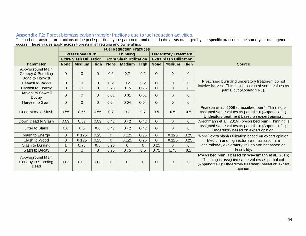
64

Appendix F2: Forest biomass carbon transfer fractions due to fuel reduction activities. The carbon transfers are fractions of the pool specified by the parameter and occur in the areas managed by the specific practice in the same year management occurs. These values apply across Forests in all regions and ownerships.

Parameter

Fuel Reduction Practices

Source

Prescribed Burn Thinning Understory Treatment

Extra Slash Utilization Extra Slash Utilization Extra Slash Utilization

None Medium High None Medium High None Medium High

Aboveground Main Canopy & Standing

Dead to Harvest 0 0 0 0.2 0.2 0.2 0 0 0

Prescribed burn and understory treatment do not involve harvest. Thinning is assigned same values as

partial cut (Appendix F1).

Harvest to Wood 0 0 0 0.2 0.2 0.2 0 0 0

Harvest to Energy 0 0 0 0.75 0.75 0.75 0 0 0

Harvest to Sawmill Decay

0 0 0 0.01 0.01 0.01 0 0 0

Harvest to Slash 0 0 0 0.04 0.04 0.04 0 0 0

Understory to Slash 0.55 0.55 0.55 0.7 0.7 0.7 0.5 0.5 0.5 Pearson et al., 2009 (prescribed burn); Thinning is assigned same values as partial cut (Appendix F1);

Understory treatment based on expert opinion.

Down Dead to Slash 0.53 0.53 0.53 0.42 0.42 0.42 0 0 0 Wiechmann et al., 2015; (prescribed burn) Thinning is assigned same values as partial cut (Appendix F1);

Understory based on expert opinion. Litter to Slash 0.6 0.6 0.6 0.42 0.42 0.42 0 0 0

Slash to Energy 0 0.125 0.25 0 0.125 0.25 0 0.125 0.25 “None” extra slash utilization based on expert opinion. Medium and high extra slash utilization are

aspirational, exploratory values and not based on feasibility.

Slash to Wood 0 0.125 0.25 0 0.125 0.25 0 0.125 0.25

Slash to Burning 1 0.75 0.5 0.25 0 0 0.25 0 0

Slash to Decay 0 0 0 0.75 0.75 0.5 0.75 0.75 0.5

Aboveground Main Canopy to Standing

Dead 0.03 0.03 0.03 0 0 0 0 0 0

Prescribed burn is based on Wiechmann et al., 2015; Thinning is assigned same values as partial cut

(Appendix F1); Understory treatment based on expert opinion.

65

Appendix F2: Forest biomass carbon transfer fractions due to fuel reduction activities. The carbon transfers are fractions of the pool specified by the parameter and occur in the areas managed by the specific practice in the same year management occurs. These values apply across Forests in all regions and ownerships.

Parameter

Fuel Reduction Practices

Source

Prescribed Burn Thinning Understory Treatment

Extra Slash Utilization Extra Slash Utilization Extra Slash Utilization

None Medium High None Medium High None Medium High

Understory to Down Dead

0.45 0.45 0.45 0.3 0.3 0.3 0.5 0.5 0.5

Prescribed burn is based on medium intensity fire from Pearson et al., 2009; Thinning is assigned same

values as partial cut (Appendix F1); Understory treatment based on expert opinion.

Soil Decay to Atmosphere

0 0 0 0.13 0.13 0.13 0 0 0

Thinning is assigned same values as partial cut (Appendix F1); Prescribed burn and understory

treatment based on expert opinion.

Belowground Main Canopy Decay to

Atmosphere 0 0 0 0.03 0.03 0.03 0 0 0

Thinning is assigned same values as partial cut (Appendix F1); Prescribed burn and understory

treatment based on expert opinion.

Belowground Main Canopy Decay to Soil

0 0 0 0.17 0.17 0.17 0 0 0

66

Appendix F3: Forest biomass carbon transfer fractions due to conversion to Cultivated Land or Urban Area. These are the fractions of carbon moved from one pool to another, to wood products, or to the atmosphere via decay, burning, or bioenergy. The transfers occur in the areas converted during the same year of conversion. These values apply across all regions and ownerships.

Parameter Dead removal from

conversion Source

Aboveground Main Canopy & Standing Dead to Harvest 1

Stewart and Nakamura, 2012; Saah et al., 2016, and Battles et al., 2014 (aboveground main canopy). Standing dead assumed to be the same fraction as

above main canopy.

Harvest to Wood 0.2

Stewart and Nakamura, 2012 Harvest to Energy 0.75

Harvest to Sawmill Decay 0.01

Harvest to Slash 0.04

Understory to Slash 0.7 Based on expert opinion.

Down Dead to Slash 0.42 Dore et al., 2016

Litter to Slash 0.42 Stewart and Nakamura, 2012

Slash to Energy 0 “None” extra slash utilization based on expert opinion. Medium and high extra slash utilization is aspirational, exploratory values and not based on feasibility. Slash to Wood 0

Slash to Burning 0.25

Slash to Decay 0.75

Aboveground Main Canopy to Standing Dead 0

Based on expert opinion.

Understory to Down Dead 0.3 Based on expert opinion.

Soil Decay to Atmosphere 0.13 Birdsey et al., 2002

Belowground Main Canopy Decay to Atmosphere 0.03

Total belowground loss based on transfer fractions for aboveground main canopy, while the partitioning to atmosphere and soil is based on Birdsey et al., 2002. The loss to soil is not added to soil, as it is assumed to be implicit in the

baseline net soil C flux.

67

Appendix G: CALAND Output variables and definitions (214 variables) These outputs are generated by running caland.r. The data are stored in an individual Excel workbook (.xls) for each scenario. Each variable corresponds to an individual worksheet within the file (in order below). There are values for each land category and each year simulated, as well as aggregated values by land type, ownership, and region at the bottom of each table.

Parameter Definition

Area (ha)

Area Land category area

Managed_area Simulated managed area – this may be different than the prescribed managed area due to land availability

Wildfire_area

Simulated wildfire area – this is the wildfire area as distributed across land categories, and the totals may be different than prescribed due to land availability

Carbon density (Mg C ha-1)

All_orgC_den Total organic carbon density (sum of the seven C pools)

All_biomass_C_den Living and dead vegetation carbon density

(All_orgC_den – Soil_orgC_den)

Above_main_C_den Main live canopy carbon density

Below_main_C_den Main live root carbon density

Understory_C_den Understory live carbon density

StandDead_C_den Standing dead carbon density

DownDead_C_den Downed dead carbon density

Litter_C_den Litter carbon density

Soil_orgC_den Soil organic carbon density

Carbon stock (Mg C)

All_orgC_stock Total organic carbon stock (sum of the seven C pools)

All_biomass_C_stock Living and dead vegetation carbon stock (All_orgC_den – Soil_orgC_den)

Above_main_C_stock Main live canopy carbon stock

Below_main_C_stock Main live root carbon stock

Understory_C_stock Understory live carbon stock

StandDead_C_stock Standing dead carbon stock

DownDead_C_stock Downed dead carbon stock

Litter_C_stock Litter carbon stock

Soil_orgC_stock Soil organic carbon stock

Wood product carbon stock (Mg C)

Total_Wood_C_stock Persistent wood product carbon stock

68

Appendix G: CALAND Output variables and definitions (214 variables) These outputs are generated by running caland.r. The data are stored in an individual Excel workbook (.xls) for each scenario. Each variable corresponds to an individual worksheet within the file (in order below). There are values for each land category and each year simulated, as well as aggregated values by land type, ownership, and region at the bottom of each table.

Parameter Definition

Wood product carbon stock (Mg C) (Cont.)

Total_Wood_CumGain_C_stock Cumulative gain in wood product carbon stock

Total_Wood_CumLoss_C_stock Cumulative loss in wood product carbon stock from decay in landfills

Total_Wood_AnnGain_C_stock Annual gain in wood product carbon stock

Total_Wood_AnnLoss_C_stock Annual loss in wood product carbon stock from decay in landfills

Manage_Wood_C_stock Persistent wood product carbon stock from forest management

Manage_TotWood_CumGain_C_stock

Cumulative gain in wood product carbon stock sourced from forest management (harvest plus extra slash utilization)

Manage_Harv2Wood_CumGain_C_stock Cumulative gain in wood product carbon stock sourced from forest management harvest

Manage_Slash2Wood_CumGain_C_stoc k Cumulative gain in wood product carbon stock sourced from forest management slash

Manage_Wood_CumLoss_C_stock

Cumulative loss in wood product carbon stock sourced from forest management, from decay in landfills

Manage_TotWood_AnnGain_C_stock

Annual gain in wood product carbon stock sourced from forest management (harvest plus extra slash utilization)

Manage_Harv2Wood_AnnGain_C_stock Annual gain in wood product carbon stock sourced from forest management harvest

Manage_Slash2Wood_AnnGain_C_stock Annual gain in wood product carbon stock sourced from forest management slash

Manage_Wood_AnnLoss_C_stock Annual loss in wood product carbon stock sourced from forest management, from decay in landfills

LCC_Wood_C_stock Persistent wood product carbon stock sourced from land cover change

LCC_TotWood_CumGain_C_stock

Cumulative gain in wood product carbon stock sourced from land cover change (harvest plus extra slash utilization)

LCC_Harv2Wood_CumGain_C_stock Cumulative gain in wood product carbon stock sourced from land cover change harvest

LCC_Slash2Wood_CumGain_C_stock Cumulative gain in wood product carbon stock sourced from land cover change slash

LCC_Wood_CumLoss_C_stock

Cumulative loss in wood product carbon stock sourced from land cover change, from decay in landfills

LCC_TotWood_AnnGain_C_stock

Annual gain in wood product carbon stock sourced from land cover change (harvest plus extra slash utilization)

LCC_Harv2Wood_AnnGain_C_stock Annual gain in wood product carbon stock sourced from land cover change harvest

69

Appendix G: CALAND Output variables and definitions (214 variables) These outputs are generated by running caland.r. The data are stored in an individual Excel workbook (.xls) for each scenario. Each variable corresponds to an individual worksheet within the file (in order below). There are values for each land category and each year simulated, as well as aggregated values by land type, ownership, and region at the bottom of each table.

Parameter Definition

Wood product carbon stock (Mg C) (Cont.)

LCC_Slash2Wood_AnnGain_C_stock Annual gain in wood product carbon stock sourced from land cover change slash

LCC_Wood_AnnLoss_C_stock Annual loss in wood product carbon stock sourced from land cover change, from decay in landfills

Land-Atmosphere carbon exchange (Mg C)

Eco_CumGain_C_stock Cumulative net gain in ecosystem carbon stock from atmosphere

Total_Atmos_CumGain_C_stock

Cumulative emissions of carbon from forest management, wildfire, land cover change, and landfill wood product decay

Manage_Atmos_CumGain_C_stock Cumulative emissions of carbon from forest management

Fire_Atmos_CumGain_C_stock Cumulative emissions of carbon from wildfire

LCC_Atmos_CumGain_C_stock Cumulative emissions of carbon from land cover change

Wood_Atmos_CumGain_C_stock Cumulative emissions of carbon from landfill wood product decay

Total_Energy2Atmos_C_stock

Cumulative emissions of carbon from biomass energy associated with forest management and land cover change

Eco_AnnGain_C_stock Annual net gain in ecosystem carbon stock from atmosphere

Total_Atmos_AnnGain_C_stock

Annual emissions of carbon from forest management, wildfire, land cover change, and landfill wood product decay

Manage_Atmos_AnnGain_C_stock Annual emissions of carbon from forest management

Fire_Atmos_AnnGain_C_stock Annual emissions of carbon from wildfire

LCC_Atmos_AnnGain_C_stock Annual emissions of carbon from land cover change

Wood_Atmos_AnnGain_C_stock Annual emissions of carbon from landfill wood product decay

Total_AnnEnergy2Atmos_C_stock

Annual emissions of carbon from biomass energy associated with forest management and land cover change

Partitioning of land-atmosphere carbon exchange (Mg C) (all carbon emissions)

Manage_Atmos_CumGain_FireC

Cumulative emissions of carbon from controlled burning due to forest management (prescribed burns and slash burning)

70

Appendix G: CALAND Output variables and definitions (214 variables) These outputs are generated by running caland.r. The data are stored in an individual Excel workbook (.xls) for each scenario. Each variable corresponds to an individual worksheet within the file (in order below). There are values for each land category and each year simulated, as well as aggregated values by land type, ownership, and region at the bottom of each table.

Parameter Definition

Partitioning of land-atmosphere carbon exchange (Mg C) (all carbon emissions) (Cont.)

Manage_Atmos_CumGain_TotEnergyC

Cumulative emissions of carbon from total bioenergy due to forest management (harvest plus extra slash utilization)

Man_Atmos_CumGain_Harv2EnergyC

Cumulative emissions of carbon from bioenergy due to Forest management harvest

Man_Atmos_CumGain_Slash2EnergyC

Cumulative emissions of carbon from bioenergy due to Forest management extra slash utilization

Manage_Atmos_CumGain_NonBurnedC Cumulative emissions of carbon from in situ and sawmill decay due to forest management (excludes wood product decay in landfills)

Fire_Atmos_CumGain_BurnedC Cumulative emissions of carbon from burning due to wildfire

Fire_Atmos_CumGain_NonBurnedC Cumulative emissions of carbon from decay due to wildfire

LCC_Atmos_CumGain_FireC Cumulative emissions of carbon from slash burning due to land cover change (default is 0)

LCC_Atmos_CumGain_TotEnergyC

Cumulative emissions of carbon from total bioenergy due to conversion of Forest to Urban Area or Cultivated Land (harvest plus extra slash utilization)

LCC_Atmos_CumGain_Harv2EnergyC Cumulative emissions of carbon from bioenergy due to harvest due to conversion of Forest to Urban Area or Cultivated Land

LCC_Atmos_CumGain_Slash2EnergyC Cumulative emissions of carbon from bioenergy due to extra slash utilization associated with conversion of Forest to Urban Area or Cultivated Land (default is 0)

LCC_Atmos_CumGain_NonBurnedC Cumulative emissions of carbon from in situ and sawmill decay due to forest management (excludes wood product decay in landfills)

Manage_Atmos_AnnGain_FireC

Annual emissions of carbon from controlled burning due to forest management (prescribed burns and slash burning)

Manage_Atmos_AnnGain_TotEnergyC

Annual emissions of carbon from total bioenergy due to forest management (harvest plus extra slash utilization)

Man_Atmos_AnnGain_Harv2EnergyC Annual emissions of carbon from bioenergy due to Forest management harvest

Man_Atmos_AnnGain_Slash2EnergyC Annual emissions of carbon from bioenergy due to Forest management extra slash utilization

Manage_Atmos_AnnGain_NonBurnedC Annual emissions of carbon from in situ and sawmill decay due to forest management (excludes wood product decay in landfills)

71

Appendix G: CALAND Output variables and definitions (214 variables) These outputs are generated by running caland.r. The data are stored in an individual Excel workbook (.xls) for each scenario. Each variable corresponds to an individual worksheet within the file (in order below). There are values for each land category and each year simulated, as well as aggregated values by land type, ownership, and region at the bottom of each table.

Parameter Definition

Partitioning of land-atmosphere carbon exchange (Mg C) (all carbon emissions) (Cont.)

Fire_Atmos_AnnGain_BurnedC Annual emissions of carbon from burning due to wildfire

Fire_Atmos_AnnGain_NonBurnedC Annual emissions of carbon from decay due to wildfire

LCC_Atmos_AnnGain_FireC Annual emissions of carbon from slash burning due to land cover change (default is 0)

LCC_Atmos_AnnGain_TotEnergyC

Annual emissions of carbon from total bioenergy due to conversion of Forest to Urban Area or Cultivated Land (harvest plus extra slash utilization)

LCC_Atmos_AnnGain_Harv2EnergyC Annual emissions of carbon from bioenergy due to harvest associated with conversion of Forest to Urban Area or Cultivated Land

LCC_Atmos_AnnGain_Slash2EnergyC Annual emissions of carbon from bioenergy due to extra slash utilization associated with conversion of Forest to Urban Area or Cultivated Land (default is 0)

LCC_Atmos_AnnGain_NonBurnC Annual emissions of carbon from in situ and sawmill decay due to land cover change (excludes wood product decay in landfills)

Man_Atmos_AnnGain_SawmillDecayC Annual emissions of carbon from sawmill decay due to forest management harvest

Man_Atmos_AnnGain_InFrstDecayC Annual emissions of carbon from in situ decay due to forest management

Man_Atmos_CumGain_SawmillDecayC Cumulative emissions of carbon from sawmill decay due to forest management harvest

Man_Atmos_CumGain_InFrstDecayC

Cumulative emissions of carbon from in situ decay of carbon due to forest management

LCC_Atmos_AnnGain_SawmillDecayC

Annual emissions of carbon from sawmill decay associated with conversion of Forest to Urban Area or Cultivated Land

LCC_Atmos_AnnGain_OnSiteDecayC

Annual emissions of carbon from in situ decay due to land cover change

LCC_Atmos_CumGain_SawmillDecayC

Cumulative emissions of carbon from sawmill decay associated with conversion of Forest to Urban Area or Cultivated Land

LCC_Atmos_CumGain_OnSiteDecayC

Cumulative emissions of carbon from in situ decay due to land cover change

Global warming potential of land-atmosphere carbon exchange (Mg CO2 eq) (land uptake is negative)

Eco_CumCO2

Cumulative ecosystem CO2 exchange (includes management and climate effects on soil and vegetation C exchange and mortality)

72

Appendix G: CALAND Output variables and definitions (214 variables) These outputs are generated by running caland.r. The data are stored in an individual Excel workbook (.xls) for each scenario. Each variable corresponds to an individual worksheet within the file (in order below). There are values for each land category and each year simulated, as well as aggregated values by land type, ownership, and region at the bottom of each table.

Parameter Definition

Global warming potential of land-atmosphere carbon exchange (Mg CO2 eq) (land uptake is negative) (Cont.)

Eco_CumCH4eq

Cumulative ecosystem CH4 exchange (includes management and climate effects on soil and vegetation C exchange and mortality)

ManTotEnergy_CumCO2 Cumulative CO2 emissions from total bioenergy due to Forest management (harvest plus extra slash utilization)

ManTotEnergy_CumCH4eq Cumulative CH4 emissions from total bioenergy due to Forest management (harvest plus extra slash utilization)

ManTotEnergy_CumBCeq Cumulative BC emissions from total bioenergy due to Forest management (harvest plus extra slash utilization)

ManHarv2Energy_CumCO2 Cumulative CO2 emissions from bioenergy due to Forest management harvest

ManHarv2Energy_CumCH4eq Cumulative CH4 emissions from bioenergy due to Forest management harvest

ManHarv2Energy_CumBCeq Cumulative BC emissions from bioenergy due to Forest management harvest

ManSlash2Energy_CumCO2 Cumulative CO2 emissions from bioenergy due to Forest management extra slash utilization

ManSlash2Energy_CumCH4eq Cumulative CH4 emissions from bioenergy due to Forest management extra slash utilization

ManSlash2Energy_CumBCeq Cumulative BC emissions from bioenergy due to Forest management extra slash utilization

ManFire_CumCO2 Cumulative CO2 emissions from controlled burning due to forest management (prescribed burns and slash burning)

ManFire_CumCH4eq Cumulative CH4 emissions from controlled burning due to forest management (prescribed burns and slash burning)

ManFire_CumBCeq Cumulative BC emissions from controlled burning due to forest management (prescribed burns and slash burning)

ManNonBurn_CumCO2 Cumulative CO2 emissions from in situ and sawmill decay due to forest management (excludes wood product decay in landfills)

ManSawmillDecay_AnnCO2 Annual CO2 emissions from sawmill decay due to Forest management

ManForestDecay_AnnCO2 Annual CO2 emissions from in situ decay due to Forest management

ManSawmillDecay_CumCO2 Cumulative CO2 emissions from sawmill decay due to Forest management

ManForestDecay_CumCO2 Cumulative CO2 emissions from in situ decay due to Forest management

73

Appendix G: CALAND Output variables and definitions (214 variables) These outputs are generated by running caland.r. The data are stored in an individual Excel workbook (.xls) for each scenario. Each variable corresponds to an individual worksheet within the file (in order below). There are values for each land category and each year simulated, as well as aggregated values by land type, ownership, and region at the bottom of each table.

Parameter Definition

Global warming potential of land-atmosphere carbon exchange (Mg CO2 eq) (land uptake is negative) (Cont.)

LCCTotEnergy_CumCO2

Cumulative CO2 emissions from total bioenergy due to conversion of Forest to Urban Area or Cultivated Land (harvest plus extra slash utilization)

LCCTotEnergy_CumCH4eq

Cumulative CH4 emissions from total bioenergy due to conversion of Forest to Urban Area or Cultivated Land (harvest plus extra slash utilization)

LCCTotEnergy_CumBCeq

Cumulative BC emissions from total bioenergy due to conversion of Forest to Urban Area or Cultivated Land (harvest plus extra slash utilization)

LCCHarv2Energy_CumCO2 Cumulative CO2 emissions from bioenergy due to harvest associated with conversion from Forest to Urban Area or Cultivated Land

LCCHarv2Energy _CumCH4eq Cumulative CH4 emissions from bioenergy due to harvest associated with conversion from Forest to Urban Area or Cultivated Land

LCCHarv2Energy_CumBCeq Cumulative BC emissions from bioenergy due to harvest associated with conversion from Forest to Urban Area or Cultivated Land

LCCSlash2Energy_CumCO2 Cumulative CO2 emissions from bioenergy due to extra slash utilization associated with conversion from Forest to Urban Area or Cultivated Land (default is 0)

LCCSlash2Energy_CumCH4eq Cumulative CH4 emissions from bioenergy due to extra slash utilization associated with conversion from Forest to Urban Area or Cultivated Land (default is 0)

LCCSlash2Energy_CumBCeq Cumulative BC emissions from bioenergy due to extra slash utilization associated with conversion from Forest to Urban Area or Cultivated Land (default is 0)

LCCFire_CumCO2 Cumulative CO2 emissions from slash burning due

to land cover change (default is 0)

LCCFire_CumCH4eq Cumulative CH4 emissions from slash burning due to land cover change (default is 0)

LCCFire_CumBCeq Cumulative BC emissions from slash burning due to land cover change (default is 0)

LCC_NonBurn_CumCO2 Cumulative CO2 emissions due land cover change, including in situ and sawmill decay (excludes landfill decay of wood products)

LCCSawmillDecay_AnnCO2

Annual CO2 emissions from sawmill decay due to land cover change associated with conversion from Forest to Urban Area or Cultivated Land

74

Appendix G: CALAND Output variables and definitions (214 variables) These outputs are generated by running caland.r. The data are stored in an individual Excel workbook (.xls) for each scenario. Each variable corresponds to an individual worksheet within the file (in order below). There are values for each land category and each year simulated, as well as aggregated values by land type, ownership, and region at the bottom of each table.

Parameter Definition

Global warming potential of land-atmosphere carbon exchange (Mg CO2 eq) (land uptake is negative) (Cont.)

LCCOnSiteDecay_AnnCO2

Annual CO2 emissions from in situ decay due to land cover change associated with land cover cahnge

LCCSawmillDecay_CumCO2

Cumulative CO2 emissions from sawmill decay due to land cover change associated with conversion from Forest to Urban Area or Cultivated Land

LCCOnSiteDecay_CumCO2 Cumulative CO2 emissions from in situ decay due to land cover change

Wildfire_Decay_AnnCO2 Annual CO2 emissions from decay due to wildfire

Wildfire_Decay_CumCO2 Cumulative CO2 emissions from decay due to wildfire

TotalEnergy_CumCO2 Cumulative CO2 emissions from all bioenergy

TotalEnergy_CumCH4eq Cumulative CH4 emissions from all bioenergy

TotalEnergy_CumBCeq Cumulative BC emissions from all bioenergy

TotalCntlFire_CumCO2

Cumulative CO2 emissions from total controlled burning (prescribed burns and slash burning) associated with forest management and land cover change

TotalCntlFire_CumCH4eq

Cumulative CH4 emissions from total controlled burning (prescribed burns and slash burning) associated with forest management and land cover change

TotalCntlFire_CumBCeq

Cumulative BC emissions from total controlled burning (prescribed burns and slash burning) associated with forest management and land cover change

Wildfire_CumCO2 Cumulative CO2 emissions from wildfire (decay plus burning)

Wildfire_CumCH4eq Cumulative CH4 emissions from wildfire

Wildfire_CumBCeq Cumulative BC emissions from wildfire

Wood_CumCO2

Cumulative CO2 emissions from all landfill decay of wood products (forest management and land cover change)

Wood_CumCH4eq

Cumulative CO2 emissions from all landfill decay of wood products (forest management and land cover change)

75

Appendix G: CALAND Output variables and definitions (214 variables) These outputs are generated by running caland.r. The data are stored in an individual Excel workbook (.xls) for each scenario. Each variable corresponds to an individual worksheet within the file (in order below). There are values for each land category and each year simulated, as well as aggregated values by land type, ownership, and region at the bottom of each table.

Parameter Definition

Global warming potential of land-atmosphere carbon exchange (Mg CO2 eq) (land uptake is negative) (Cont.)

Eco_AnnCO2

Annual ecosystem CO2 exchange (includes management and climate effects on soil and vegetation C exchange and mortality)

Eco_AnnCH4eq

Annual ecosystem CH4 exchange (includes management and climate effects on soil and vegetation C exchange and mortality)

ManTotEnergy_AnnCO2 Annual CO2 emissions from total bioenergy due to Forest management (harvest plus extra slash utilization)

ManTotEnergy_AnnCH4eq Annual CH4 emissions from total bioenergy due to Forest management (harvest plus extra slash utilization)

ManTotEnergy_AnnBCeq Annual BC emissions from total bioenergy due to Forest management (harvest plus extra slash utilization)

ManHarv2Energy_AnnCO2 Annual CO2 emissions from bioenergy due to Forest management harvest

ManHarv2Energy_AnnCH4eq Annual CH4 emissions from bioenergy due to Forest management harvest

ManHarv2Energy_AnnBCeq Annual BC emissions from bioenergy due to Forest management harvest

ManSlash2Energy_AnnCO2 Annual CO2 emissions from bioenergy due to Forest management extra slash utilization

ManSlash2Energy_AnnCH4eq Annual CH4 emissions from bioenergy due to Forest management extra slash utilization

ManSlash2Energy_AnnBCeq Annual BC emissions from bioenergy due to Forest management extra slash utilization

ManFire_AnnCO2 Annual CO2 emissions from from controlled burning due to forest management (prescribed burns and slash burning)

ManFire_AnnCH4eq Annual CH4 emissions from controlled burning due to forest management (prescribed burns and slash burning)

ManFire_AnnBCeq Annual BC emissions from controlled burning due to forest management (prescribed burns and slash burning)

ManNonBurn_AnnCO2

Annual CO2 emissions from in situ and sawmill decay due to forest management (excludes wood product decay in landfills)

LCCTotEnergy_AnnCO2

Annual CO2 emissions from bioenergy due to conversion from Forest to Urban Area or Cultivated Land from Forest (harvest plus extra slash utilization)

76

Appendix G: CALAND Output variables and definitions (214 variables) These outputs are generated by running caland.r. The data are stored in an individual Excel workbook (.xls) for each scenario. Each variable corresponds to an individual worksheet within the file (in order below). There are values for each land category and each year simulated, as well as aggregated values by land type, ownership, and region at the bottom of each table.

Parameter Definition

Global warming potential of land-atmosphere carbon exchange (Mg CO2 eq) (land uptake is negative) (Cont.)

LCCTotEnergy_AnnCH4eq

Annual CH4 emissions from bioenergy due to conversion from Forest to Urban Area or Cultivated Land from Forest (harvest plus extra slash utilization)

LCCTotEnergy_AnnBCeq

Annual BC emissions from bioenergy due to conversion from Forest to Urban Area or Cultivated Land from Forest (harvest plus extra slash utilization)

LCCHarv2Energy_AnnCO2

Cumulative CO2 emissions from bioenergy due to harvest associated with conversion from Forest to Urban Area or Cultivated Land

LCCHarv2Energy_AnnCH4eq

Cumulative CH4 emissions from bioenergy due to harvest associated with conversion from Forest to Urban Area or Cultivated Land

LCCHarv2Energy_AnnBCeq

Cumulative BC emissions from bioenergy due to harvest associated with conversion from Forest to Urban Area or Cultivated Land

LCCSlash2Energy_AnnCO2

Cumulative CO2 emissions from bioenergy due to extra slash utilization associated with conversion from Forest to Urban Area or Cultivated Land (default is 0)

LCCSlash2Energy_AnnCH4eq

Cumulative CH4 emissions from bioenergy due to extra slash utilization associated with conversion from Forest to Urban Area or Cultivated Land (default is 0)

LCCSlash2Energy_AnnBCeq

Cumulative BC emissions from bioenergy due to extra slash utilization associated with conversion from Forest to Urban Area or Cultivated Land (default is 0)

LCCFire_AnnCO2 Cumulative CO2 emissions from slash burning due to land cover change (default is 0)

LCCFire_AnnCH4eq Cumulative CH4 emissions from slash burning due to land cover change (default is 0)

LCCFire_AnnBCeq Cumulative BC emissions from slash burning due to

land cover change (default is 0)

LCC_NonBurn_AnnCO2

Annual CO2 emissions due land cover change, including in situ and sawmill decay (excludes landfill

decay of wood products)

TotalEnergy_AnnCO2 Annual CO2 emissions from all bioenergy

TotalEnergy_AnnCH4eq Annual CH4 emissions from all bioenergy

TotalEnergy_AnnBCeq Annual BC emissions from all bioenergy

77

Appendix G: CALAND Output variables and definitions (214 variables) These outputs are generated by running caland.r. The data are stored in an individual Excel workbook (.xls) for each scenario. Each variable corresponds to an individual worksheet within the file (in order below). There are values for each land category and each year simulated, as well as aggregated values by land type, ownership, and region at the bottom of each table.

Parameter Definition

Global warming potential of land-atmosphere carbon exchange (Mg CO2 eq) (land uptake is negative) (Cont.)

TotalCntlFire_AnnCO2

Annual CO2 emissions from total controlled burning (prescribed burns and slash burning) associated

with forest management and land cover change

TotalCntlFire_AnnCH4eq

Annual CH4 emissions from total controlled burning (prescribed burns and slash burning) associated

with forest management and land cover change

TotalCntlFire_AnnBCeq

Annual BC emissions from total controlled burning

(prescribed burns and slash burning) associated with forest management and land cover change

Wildfire_AnnCO2 Annual CO2 emissions from wildfire (decay plus

burning)

Wildfire_AnnCH4eq Annual CH4 emissions from wildfire

Wildfire_AnnBCeq Annual BC emissions from wildfire

Wood_AnnCO2

Annual CO2 emissions from all landfill decay of wood products (forest management and land cover

change)

Wood_AnnCH4eq

Annual CO2 emissions from all landfill decay of wood products (forest management and land cover

change)

Total_CumCO2 Cumulative CO2 exchange from all sources

Total_CumCH4eq Cumulative CH4 exchange from all sources

Total_CumBCeq Cumulative BC exchange from all sources

Total_AnnCO2 Annual CO2 exchange from all sources

Total_AnnCH4eq Annual CH4 exchange from all sources

Total_AnnBCeq Annual BC exchange from all sources

TotalWood_CumCO2eq_all Cumulative emissions of CO2 and CH4 from landfill

decay of wood products

TotalWood_AnnCO2eq_all Annual emissions of CO2 and CH4 from landfill

decay of wood products

TotalNonBurn_CumCO2eq_all Cumulative exchange of CO2 and CH4 from all sources excluding controlled burning and wildfire

TotalFire_CumCO2eq_all

Cumulative emissions of CO2, CH4, and BC from controlled burning (prescribed burn and slash

burning) and wildfire

78

Appendix G: CALAND Output variables and definitions (214 variables) These outputs are generated by running caland.r. The data are stored in an individual Excel workbook (.xls) for each scenario. Each variable corresponds to an individual worksheet within the file (in order below). There are values for each land category and each year simulated, as well as aggregated values by land type, ownership, and region at the bottom of each table.

Parameter Definition

Global warming potential of land-atmosphere carbon exchange (Mg CO2 eq) (land uptake is negative) (Cont.)

TotalEnergy_CumCO2eq_all

Cumulative emissions of CO2, CH4, and BC from all bioenergy (forest management and land cover

change)

TotalNonBurn_AnnCO2eq_all Annual exchange of CO2 and CH4 from all sources excluding all controlled burning and wildfire

TotalFire_AnnCO2eq_all

Annual emissions of CO2, CH4, and BC from controlled burning (prescribed burn and slash

burning) and wildfire

TotalEnergy_AnnCO2eq_all

Annual emissions of CO2, CH4, and BC from all bioenergy (forest management and land cover

change)

TotalBurn_CumCO2eq_all Cumulative exchange of CO2, CH4, and BC from all

controlled burning and wildfire

TotalBurn_AnnCO2eq_all Annual exchange of CO2, CH4, and BC from all controlled burning and wildfire

Total_CumCO2eq_all Cumulative exchange of CO2, CH4, and BC from all sources

Total_AnnCO2eq_all Annual exchange of CO2, CH4, and BC from all sources

Additional partitioning of BC-C emissions (Mg C)

ManFire_CumBCC

Cumulative emissions of BC from controlled burning

due to Forest management (prescribed burn and slash burning)

ManTotEnergy_CumBCC

Cumulative emissions of BC from total bioenergy due to Forest management (harvest plus extra slash

utilization)

ManHarv2Energy_CumBCC Cumulative emissions of BC from bioenergy due to Forest management harvest

ManSlash2Energy_CumBCC Cumulative emissions of BC from bioenergy due to Forest management extra slash utilization

LCCFire_CumBCC Cumulative BC emissions from slash burning due to

land cover change (default is 0)

LCCTotEnergy_CumBCC

Cumulative BC emissions from bioenergy due to

conversion from Forest to Urban Area or Cultivated Land from Forest (harvest plus extra slash

utilization)

LCCHarv2Energy_CumBCC

Cumulative BC emissions from bioenergy due to harvest associated with conversion from Forest to

Urban Area or Cultivated Land

LCCSlash2Energy_CumBCC

Cumulative BC emissions from bioenergy due to

extra slash utilization associated with conversion from Forest to Urban Area or Cultivated Land

(default is 0)

79

Appendix G: CALAND Output variables and definitions (214 variables) These outputs are generated by running caland.r. The data are stored in an individual Excel workbook (.xls) for each scenario. Each variable corresponds to an individual worksheet within the file (in order below). There are values for each land category and each year simulated, as well as aggregated values by land type, ownership, and region at the bottom of each table.

Parameter Definition

Additional partitioning of BC-C emissions (Mg C) (Cont.)

Wildfire_CumBCC Cumulative emissions of BC from wildfire

ManFire_AnnBCC Annual emissions of BC from wildfire

ManTotEnergy_AnnBCC

Annual emissions of BC from controlled burning due to Forest management (prescribed burn and slash

burning)

ManHarv2Energy_AnnBCC

Annual emissions of BC from total bioenergy due to Forest management (harvest plus extra slash

utilization)

ManSlash2Energy_AnnBCC Annual emissions of BC from bioenergy due to

Forest management harvest

LCCFire_AnnBCC Annual emissions of BC from bioenergy due to Forest management extra slash utilization

LCCTotEnergy_AnnBCC Annual BC emissions from slash burning due to land cover change (default is 0)

LCCHarv2Energy_AnnBCC

Annual BC emissions from bioenergy due to

conversion from Forest to Urban Area or Cultivated Land from Forest (harvest plus extra slash

utilization)

LCCSlash2Energy_AnnBCC

Annual BC emissions from bioenergy due to harvest

associated with conversion from Forest to Urban Area or Cultivated Land

Wildfire_AnnBCC

Annual BC emissions from bioenergy due to extra

slash utilization associated with conversion from Forest to Urban Area or Cultivated Land (default is

0)

80

References

Battles, J.J., Gonzalez, P., Robards, T., Collins, B.M., and Saah, D.S., (2014). California

forest and rangeland greenhouse gas inventory development final report. California Air

Resources Board Agreement 10-778, Jan 2014.

Birdsey, R.A. and Lewis, G.M. (2002). Carbon in U.S. forests and wood products, 1987-1997:

state-by-state estimates. General Technical Report NE-310, USFS, Northeastern Research

Station.

Bond-Lamberty, B., Calvin, K., Jones, A.D., Mao, J., Patel, P., Shi, X.Y., Thomson, A., Thornton,

P., Zhou, Y. (2014). On linking an Earth system model to the equilibrium carbon representation of

an economically optimizing land use model. Geoscientific Model Development, 7:2545-2555.

DOI: 10.5194/gmd-7-2545-2014.

Brown, S., Pearson, T., Dushku, A., Kadyzewski, J., and Qi, Y. (2004). Baseline greenhouse gas

emissions for forest, range, and agricultural lands in California. Winrock International, for the

California Energy Commision. PIER Energy Related Environmental Research. 500-04-069F.

CAL FIRE (2016). Program Environmental Impact Report for the Vegetation Treatment

Program. Chapter 5: Cumulative effects analysis. Draft, March 2016.

Callaway, J.C., Borgnis, E.L., Turner, R.E., and Milan, C.S. (2012). Carbon sequestration

and sediment accretion in San Francisco Bay tidal wetlands. Estuaries and Coasts, 35:1163-

1181. DOI: 10.1007/s12237-012-9508-9.

CARB, (2016). California’s 2000-2014 Greenhouse Gas Emission Inventory: Technical

Support Document. State of California Air Resources Board, Air Quality Planning and

Science Division, September 2016.

Carreras-Sospedra, M., MacKinnon, M., Dabdub, D., and Williams, R., (2015). Assessment of

the emissions and energy impacts of biomass and biogas use in California, CA ARB report,

agreement #11-307, Feb. 27, 2015.

CCED (2015). California Conservation Easement Database, version 2015a: Database

manual, April 2015. Greeninfo Network.

Chmura, G.L., Anisfeld, S.C., Cahoon, D.R., and Lynch, J.C. (2003). Global carbon sequestration

in tidal, saline wetland soils. Gobal Biogeochemical Cycles, 17(4):1111. DOI:

10.1029/2002GB001917.

Christensen, G.A, Grray, A.N., Kuegler, O., Tase, N.A., Rosenburg, M. (2017). AB 1504

California forest ecosystem and harvested wood product carbon inventory: 2006-2015. Final

Report. California Department of Forestry and Fire Protection agreement no. 7CA02025.

Sacramento, CA: California Department of Forestry and Fire Protection and California Board of

Forestry and Fire Protection. 390p. Christensen et al., 2017

Christensen, Glenn A.; Waddell, Karen L.; Stanton, Sharon M.; Kuegler, Olaf, tech.eds. 2016.

California’s forest resources: Forest Inventory and Analysis, 2001–2010. Gen. Tech. Rep. PNW-

GTR-913. Portland, OR: U.S. Department of Agriculture, Forest Service, Pacific Northwest

81

Research Station. 293 p.

CNRA (2017). California Forest Carbon Plan: Managing our forest landscapes in a changing

climate. Draft, January 20, 2017. CNRA, CALFIRE, CAL EPA.

http://www.fire.ca.gov/fcat/downloads/California%20Forest%20Carbon%20Plan

%20Draft%20for%20Public%20Review_Jan17.pdf.

Collins, W.D., Craig, A.P., Truesdale, J.E., Di Vittorio, A.V., Jones, A.D., Bond-Lamberty, B.,

Calvin, K.V., Edmonds, J.A., Kim, S.H., Thomson, A.M., Patel, P., Zhou, Y., Mao, J., Shi, X.,

Thornton, P.E., Chini, L.P., Hurtt, G.C. (2015). The integrated Earth system model version 1:

formulation and functionality. Geoscientific Model Development, 8:2203-2219. DOI:

10.5194/gmd-8-2203-2015.

Collins, B.M., Stevens, J.T., Miller, J.D., Stephens, S.L., Brown, P.M., North, M.P. (2017).

Alternative characterization of forest fire regimes: incorporating spatial patterns. Landscape

Ecology, 32:1543-1552. DOI: 10.1007/s10980-017-0528-5.

Davidson, E.A. and Ackerman, I.L. (1993). Changes in soil carbon inventories following

cultivation of previously untilled soils. Biogeochemistry, 20(3):161-193.

Deverel, S., personal communication, Principal Hydrologist, Hydrofocus, Inc. Dingman, J.,

personal communication, Staff, California Air Resources Board

Dore, S., Fry, D.L., Collins, B.M., Vargas, R., York, R.A., Stephens, S.L. (2016). Management

impacts on carbon dynamics in a Sierra Nevada mixed conifer forest. PLOS ONE,

11(2):e0150256. DOI: 10.1371/journal.pone.0150256.

Drexler, J.Z., Fuller, C.C., Orlando, J., and Moore, P.E. (2015). Recent rates of carbon

accumulation in montane fens of Yosemite National Park, California,

U.S.A. Arctic, Antarctic, and Alpine Research, 47(4):657-669. DOI:

10.1657/AAAR0015-002.

Evans, R.D., Koyama, A., Sonderegger, D.L., Charlet, T.N., Newingham B.A., Fenstermaker,

L.F., Harlow, B., Jin, V.L., Ogle, K., Smith, S.D., and Nowak R.S. (2014). Greater ecosystem

carbon in the Mojave Desert after ten years exposure to elevated CO2. Nature Climate Change.

DOI: 10.1038/NCLIMATE2184.

Forster, P., V. Ramaswamy, P. Artaxo, T. Berntsen, R. Betts, D.W. Fahey, J. Haywood, J.

Lean, D.C. Lowe, G. Myhre, J. Nganga, R. Prinn, G. Raga,

M. Schulz, and R. Van Dorland (2007), 2007: Changes in atmospheric constituents and in

radiative forcing, in: Climate change 2007: The physical science basis. Contribution of Working

Group I to the Fourth Assessment Report of the Intergovernmental Panel on Climate Change,

edited by S. Solomon, D. Qin, M. Manning, Z. Chen, M. Marquis, K.B. Averyt, M.Tignor, and

H.L. Miller Cambridge Univ. Press, Cambridge, UK, and New York. p. 129–234.

FRAP (2010). Chapter 1.2: Sustainable working forests and rangelands. In: California’s

forests and rangelands: 2010 assessment. CALFIRE FRAP.

Gonzalez, P., Battles, J.J., Collins, B.M., Robards, T., Saah, D.S. (2015). Aboveground live

82

carbon stock changes of California wildland ecosystems, 2001- 2010. Forest Ecology and

Management, 348:68-77. DOI: 10.1016/j.foreco.2015.03.040.

Gwynne, B., personal communication, Senior Environmental Scientist, California Department of

Conservation

Harmon, M.E., Cromack, K., Smith, B.G. (1987). Coarse woody debris in mixed-conifer forests,

Sequoia National Park, California. Canadian Journal of Forest Research, 17:1265-1272.

Hastings, S.J., Oechel, W.C., and Muhlia-Melo, A. (2005). Diurnal, seasonal and annual variation

in the net ecosystem CO2 exchange of a desert shrub community (Sarcocaulescent) in Baja

California, Mexico. Global Change Biology, 11:927-939. DOI: 10.1111/j.1365-

2486.2005.00951.x.

Hatala, J.A., Detto, M., Sonnentag, O., Deverel, S.J., Verfaillie, J., Baldocchi,

D.D. (2012). Greenhouse gas (CO2, CH4, H2O) fluxes from drained and flooded agricultural

peatlands in the Sacramento-San Joaquin Delta. Agriculture, Ecosystems, and Environment,

150:1-18. DOI: 10.1016/j.agee.2012.01.009.

Hudiburg, T., Law, B., Turner, D.P., Campbell, J., Donato, D., and Duane, M. (2009). Carbon

dynamics of Oregon and Northern California forests and potential land-based carbon storage.

Ecological Applications, 19(1):163-180.

IPCC (2006a). 2006 IPCC Guidelines for National Greenhouse Gas Inventories. Volume 4:

Agriculture, Forestry and Other Land use. Chapter 12: Harvested Wood Products.

IPCC (2006b). 2006 IPCC Guidelines for National Greenhouse Gas Inventories. Volume 5:

Waste. Chapter 3: Solid Waste Disposal.

Jenkins, B.M. et al. (1996) Atmospheric Pollutant Emission Factors from Open Burning of

Agricultural and Forest Biomass by Wind Tunnel Simulations, Vol. 1-3. Final Report, ARB

contract A932-126. University of California, Davis, CA.

Jenkins, J.C., Chojnacky, D.C., Heath, L.S., and Birdsey, R.A. (2003). National- scale biomass

estimators for United States tree species. Forest Science, 49(1):12-35.

Knox, S.H., C. Sturtevant, J.H. Matthes, L. Koteen, J. Verfaillie, and D. Baldocchi (2015).

Agricultural peatland restoration: effects of land-use change on greenhouse gas (CO2 and CH4)

fluxes in the Sacramento-San Joaquin Delta.

Global Change Biology, 21:750-765. DOI: 10.1111/gcb.12745.

Ko, J., personal communication, Climate Change and Ecosystem Services Program Lead,

U.S. Forest Service

Kong, A.Y.Y., Six, J., Bryant, D.C., Denison, R.F., van Kessel, C. (2005). The relationship

between carbon input, aggregation, and soil organic carbon stabilization in sustainable cropping

systems. Soil Science Society of America Journal, 69:1078-1085 doi: 10.2136/sssaj2004.0215.

Kroodsma, D.A. and Field, C.B. (2006). Carbon sequestration in California agriculture,

83

1980-2000. Ecological applications, 16(5):1975-1985.

Sleeter, B.M., Lydersen, J.M., Collins, B.M., Brooks, M.L., Matchett, J.R., Shive, K.L.,

Povak, N.A., Kane, V.R., Smith, D.F. (2017). Evidence of fuels management and fire weather

influencing fire severity in an extreme fire event. Ecological Applications, 27(7):2013-2030.

T.S. Wilson, E. Sharygrin, and J.T. Sherba (2017) Future scenarios of land change based on

empirical data and demographic trends. Earth’s Future, 5:1068-1083,

https://doi.org/10.1002/2017EF000560.

Ma, S., Baldocchi, D.D., Xu, L., and Hehn, T. (2007). Inter-annual variability in carbon

dioxide exchange of an oak/grass savanna and open grassland in California. Agricultural and

Forest Meteorology, 147:157-171. DOI: 10.1016/j.agrformet.2007.07.008.

McIver, C.P., Meek, J.P., Scudder, M.G., Sorenson, C.B., Morgan, T.A., Christensen, G.A.

(2015). California’s forest products industry and timber harvest, 2012. Gen. Tech. Rep. PNW-

GTR-908. Portland, OR: U.S. Department of Agriculture, Forest Service, Pacific Northwest

Research Station. 49p.

McPherson, E.G., Xiao, Q., van Doorn, N.S., de Geode, J., Bjorkman, J., Hollander, A., Boynton,

R.M., Quinn, J., Thorne, J.H., (2017). The structure, function and value of urban forests in

California communities. Urban Forestry and Urban Greening, 28:43-53.

Miller, J.D., Safford, H.D. (2012). Trends in wildfire severity: 1984 to 2010 in the Sierra Nevada,

Modoc Plateau, and Southern Cascades, California, USA. Fire Ecology, 8(3):41-57. DOI:

10.4996/fireecology.0803041.

Miller, J.D., Safford, H.D., Crimmins, M., and Thode, A.E. (2009). Quantitative evidence for

increasing forest fire severity in the Sierra Nevada and Southern Cascade mountains, California

and Nevada, USA. Ecosystems, 12:16-32. DOI: 10.1007/s10021-008-9201-9.

Mitchell, J.P., Shrestha, A., Horwath, W.R., Southard, R.J., Madden, N., Veenstra, J., and

Munk, D.S. (2015). Tillage and cover cropping affect crop yields and soil carbon in the San

Joaquin Valley, California. Agronomy Journal, 107:588-596. DOI: 10.2134/agronj14.0415.

Mcleod, E., G.L. Chmura, S. Bouillon, R. Salm, M. Bjork, C.M. Duarte, C.E. Lovelock,

W.H. Schlesinger, and B.R. Silliman (2011). A blueprint for blue carbon: toward an

improved understanding of the role of vegetated coastal habitats in sequestering CO2.

Frontiers in Ecology and the Environment, 9(10):552-560. DOI: 10.1890/110004.

Myhre, G., D. Shindell, F.-M. Bréon, W. Collins, J. Fuglestvedt, J. Huang, D. Koch, J.-F.

Lamarque, D. Lee, B. Mendoza, T. Nakajima, A. Robock, G. Stephens, T. Takemura and H.

Zhang (2013), 2013: Anthropogenic and Natural Radiative Forcing, in: Climate Change 2013:

The Physical Science Basis.

Contribution of Working Group I to the Fifth Assessment Report of the Intergovernmental Panel

on Climate Change, edited by Stocker, T.F., D. Qin, G.-

K. Plattner, M. Tignor, S.K. Allen, J. Boschung, A. Nauels, Y. Xia, V. Bex and

P.M. Midgley, Cambridge University Press, Cambridge, UK, and New York, NY, USA.

84

NOAA (NOAA). California eelgrass mitigation policy and implementing guidelines.

NOAA Fisheries, West Coast Region, Oct. 2014.

Pearson, T., Brown, S., and Netzer, N. (2009). Baseline greenhouse gas emissions and

removals for forests and rangelands in California. Winrock International, for the

California Energy Commission, PIER Energy-Related Environemntal Research.

Pouyat, R.V., Yesilonis, I.D., and Nowak, D.J. (2006). Carbon storage by urban soils in the

United States. Journal of Environmental Quality, 35:1566-1575. DOI: 10.2134/jeq2005.0215.

Powers, R.F., Busse, M.D., McFarlane, K.J., Zhang, J., and Young, D.H. (2013). Long-term

effects of silviculture on soil carbon storage: does vegetation control make a difference?

Forestry, 86:47-58. DOI: 10.1093/forestry/cps067.

Quideau, S.A., Graham, R.C., Chadwick, O.A., and Wood, H.B. (1998). Organic carbon

sequestration under chaparral and pine after four decades of soil development. Geoderma,

83:227-242.

Robards, T. and Nickerson J. (2013). Appendix 3: Carbon dioxide (CO2) emissions estimates

associated with silviculture applications for California forests. In: Battles, J.J., Gonzalez, P.,

Robards, T., Collins, B.M., and Saah, D.S., California forest and rangeland greenhouse gas

inventory development final report. California Air Resources Board Agreement 10-778, Jan 2014.

Ryals, R. and Silver, W.L. (2013). Effects of organic matter amendments on net primary

productivity and greenhouse gas emissions in annual grasslands.

Ecological Applications, 23(1):46-59.

Ryals, R., Hartman, M.D., Parton, W.J., DeLonge, M.S., and Silver, W.L. (2015). Long-term

climate change mitigation potential with organic matter management on grasslands. Ecological

Applications, 25(2):531-545.

Saah D., J. Battles, J. Gunn, T. Buchholz, D. Schmidt, G. Roller, and S. Romsos. 2016. Technical

improvements to the greenhouse gas (GHG) inventory for California forests and other lands.

Submitted to: California Air Resources Board, Agreement #14-757. 55 pages.

Silver, W.L., Ryals, R., and Eviner, V. (2010). Soil carbon pools in California’s annual grassland

ecosystems. Rangeland Ecology and Management, 63(1):128- 136. DOI: 10.2111/REM-D-09-

00106.1.

Wilson, T.S., Sharygin, E., Sherba, J.T. (2017). Future scenarios of land change based on empirical

data and demographic trends. Earth’s Future, 5:1068-1083. https://doi.org/10.1002/2017EF000560.

Stevens, J.T., Collins, B.M., Miller, J.D., North, M.P., Stephens, S.L. (2017). Changing spatial

patterns of stand-replacing fire in California conifer forests. Forest Ecology and Management,

406:28-36.

Stewart, W.C. and Nakamura, G.M. (2012). California: Linking harvests to the US greenhouse

gas inventory. Forest Products Journal, 62(5):340-353.

85

Turk, J.K. and Graham, R.C. (2009). Soil carbon and nitrogen accumulation in a forested debris

flow chronosequence, California. Soil Science Society of America Journal, 73:1504-1509. DOI:

10.2136/sssaj2008.0106.

USDA (2014). Gridded soil survey geographic (gSSURGO) database: User guide. Version 1.1,

April 2014, National Soil Survey Center, National Geospatial Center of Excellence, Natural

Resources Conservation Service.

https://www.nrcs.usda.gov/wps/portal/nrcs/detail/soils/survey/geo/?cid=nrcs142p 2_053628.

Westerling, A.L. (2018). Wildfire simulations for California’s Fourth Climate Change

Assessment: Projecting changes in extreme wildfire events with a warming climate. California’s

Fourth Climate Change Assessment, California Energy Commission. Publication Number:

CCCA4-CEC-2018-014.

Wiechmann, M.L., Hurteau, M.D., North, M.P., Koch, G.W., Jerabkova, L. (2015). The carbon

balance of reducing wildfire risk and restoring process: an analysis of 10-year post-treatment

carbon dynamics in a mixed-conifer forest. Climatic Change, 132:709-719. DOI:

10.1007/s10584-015-1450-y.

Wilson, T., Woodall, C.W., and Griffith, D.M. (2013). Imputing forest carbon stock estimates

from inventory plots to a nationally continuous coverage. Carbon Balance and Management, 8:1.

http://www.cbmjournal.com/content/8/1/1.

Wohlfahrt, G., Fenstermaker, L.F., and Arnone, J.A. III (2008). Large annual net ecosystem CO2

uptake of a Mojave Desert ecosystem. Global Change Biology, 14:1475:1487. DOI:

10.1111/j.1365-2468.2008.01593.x.

Wu, L., Wood, Y., Jiang, P., Li, L., Pan, G., Lu, J., Change, A.C., and Enloe, H.A. (2008).

Carbon sequestration and dynamics of two irrigated agricultural soils in California. Soil Science

Society of America Journal, 72:808-814. DOI: 10.2136/sssaj2007.0074.

86

Extended Bibliography for CALAND

Black, T.A., J.W. Harden (1995). Effect of timber harvest on soil carbon storage at Blodgett

Experimental Forest, California. Canadian Journal of Forest Research, 25:1385-1396.

Blankinship, J.C., S.C. Hart (2014). Hydrological control of greenhouse gas fluxes in a

Sierra Nevada subalpine meadow. Arctic, Antarctic, and Alpine Research, 46(2):355-364.

Byrnes, R., V. Eviner, E. Kebreab, W.R. Horwath, L. Jackson, B. Jenkins, S. Kaffka, A. Kerr, J.

Lewis, F. Mitloehner, J. Mitchell, K. Scow (2016). Leveraging research to inform California

climate scoping plan: agriculture and working lands sectors. UC Davis World Food Center

report to CA ARB.

De Gryze, S., A. Wolf, S.R. Kaffka, J. Mitchell, D.E. Rolston, S.R. Temple, J. Lee,

J. Six (2010). Simulating greenhouse gas budgets of four California cropping systems under

conventional and alternative management. Ecological Applications, 20(7):1805-1819.

DeLonge, M.S., Ryals, R. and Silver, W.L. 2013. A Lifecycle Model to Evaluate Carbon

Sequestration Potential and Greenhouse Gas Dynamics of Managed Grasslands. Ecosystems,

16: 962–979.

Drexler, J.Z., C.C. Fuller, J.Orlando, P.E. Moore (2015). Recent rates of carbon accumulation in

montane fens of Yosemite National Park, California, USA. Arctic, Antarctic, and Alpine

Research, 47(4):657-669.

Gaman, T. (2008). Oaks 2040: Carbon resources in California oak woodlands. An inventory

of carbon and California oaks. California Oak Foundation.

Gaman, T., J. Firman (2006). Oaks 2040: The status and future of oaks in California.

General Technical Report PSW-GTR-217.

Jasoni, R.L., S.D. Smith, J.A. Arnone III (2005). Net ecosystem CO2 exchange in Mojave Desert

shrublands during the eighth year of exposure to elevated CO2.

Global Change Biology, 11:749-756.

Koteen, L.E., N. Raz-Yaseef, D.D. Baldocchi (2015). Spatial heterogeneity of fine root biomass

and soil carbon in a California oak savanna illuminates plant functional strategy across periods of

high and low resource supply.

Ecohydrology, 8:294-308.

Luo, H., Oechel, W.C., Hastings, S.J., Zulueta, R., Qian, Y. and Kwon, H. 2007. Mature semiarid

chaparral ecosystems can be a significant sink for atmospheric carbon dioxide. Glob. Chang.

Biol., 13: 386–396.

McIntyre, P.J., J.H. Thorne, C.R. Dolanc, A.L. Flint, L.E. Flint, M. Kelley, D.D. Ackerly

(2015). Twentieth-century shifts in forest structure in California: Denser forests, smaller trees,

and increased dominance of oaks. Proceedings of the National Academy of Sciences Early

Edition, 6pp. doi: 10.1073/pnas.1410186112.

McPherson, E.G., Q. Xiao, E. Aguaron (2013). A new approach to quantify and map carbon

87

stored, sequestered and emissions avoided by urban forests.

Landscape and Urban Planning, 120:70-84.

Norton, J.B., L.J. Jungst, U. Norton, H.R. Olsen, K.W. Tate, W.R. Horwath (2011). Soil

carbon and nitrogen storage in upper montane riparian meadows. Ecosystems, 14(8):1217-

1231.

Norton, J.B., H.R. Olsen, L.J. Jungst, D.E. Legg, W.R. Horwath (2014). Soil carbon and

nitrogen storage in alluvial wet meadows of the southern Sierra Nevada mountains, USA.

Journal of Soils Sediments, 10pp. doi: 10.1007/s11368-013-0797-9.

Smith, J.E., L.S. Heath, J.C. Jenkins (2003). Forest volume-to-biomass models and estimates of

mass for live and standing dead trees of U.S. forests. General Technical Report NE-298. USDA

FS.

Smith, J.E., L.S. Heath, K.E. Skog, R.A. Birdsey (2006). Methods for calculating forest

ecosystem and harvested carbon with standard estimates for forest types of the United States.

General Technical Report NE-343. USDA FS.

Smukler, S.M., S. Sanchez-Moreno, S.J. Fonte, H. Ferris, K. Klonsky, A.T. O’Geen, K.M.

Scow, K.L. Steenwerth, L.E. Jackson (2010). Biodiversity and multiple ecosystem functions in

an organic farmscape. Agriculture, Ecosystems and Environment, 139:80-97.

Stephens, S.L., R.E.J. Boerner, J.J. Modhaddas, E.E.Y. Moghaddas, B.M. Collins, C.B.

Dow, C. Edminster, C.E. Fiedler, D.L. Fry, B.R., Hartsough, J.E. Keeley, E.E. Knapp, J.D.

McIver, C.N. Skinner, A. Youngblood (2012). Fuel treatment impacts on estimated wildfire

carbon loss from forests in Montana, Oregon, California, and Arizona. Ecoshpere, 3(5):38.

Teh, Y.A., W.L. Silver, O. Sonnentag, M. Detto, M. Kelly, D.D. Baldocchi (2011). Large

greenhouse gas emissions from a temperate peatland pasture.

Ecosystems, 14(2):311-325.

Welch, K.R., H.D. Safford, T.P. Young (2016). Predicting conifer establishment post wildfire

in mixed conifer forests of the North American Mediterranean- climate zone. Ecospere,

7(12):e01609.

Williams, J.N., A.D. Hollander, A.T. O’Geen, L.A. Thrupp, R. Hanifin, K. Steenwerth, G.

McGouty, L.E. Jackson (2011). Assessment of carbon in woody plants and soil across a

vineyard-woodland landscape. Carbon Balance and Management, 6:11.

Wohlfahrt, G., L.F. Fensermaker, J.A. Arnone III (2008). Large annual net ecosystem CO2

uptake of a Mojave Desert ecosystem. Global Change Biology, 14:1475-1487.

Wu, L., A.C. Chang, B. McCullough-Sanden, K.M. Bali (2006). Quantitative and qualitative

assessment of soil organic carbon in native and cropland soils in California. Kearny Foundation

of Soil Science: Soil carbon and California’s Terrestrial Ecosystems, Final Report: 2001033.

Xu, L., D.D. Baldocchi (2004). Seasonal variation in carbon dioxide exchange over a

Mediterranean annual grassland in California. Agricultural and Forest Meteorology, 1232:79-

96.