Can the brain use waves to solve planningproblems?

Henry Powell1,2, Mathias Winkel1, Alexander V. Hopp1, andHelmut Linde1

1Merck KGaA, Darmstadt, Germany2University of Glasgow, Scotland

October 12, 2021

A variety of behaviors like spatial navigation or bodily motion can be formulatedas graph traversal problems through cognitive maps. We present a neural networkmodel which can solve such tasks and is compatible with a broad range of em-pirical findings about the mammalian neocortex and hippocampus. The neuronsand synaptic connections in the model represent structures that can result fromself-organization into a cognitive map via Hebbian learning, i.e. into a graph inwhich each neuron represents a point of some abstract task-relevant manifold andthe recurrent connections encode a distance metric on the manifold. Graph traver-sal problems are solved by wave-like activation patterns which travel through therecurrent network and guide a localized peak of activity onto a path from somestarting position to a target state.

1

arX

iv:2

110.

0515

8v1

[cs

.NE

] 1

1 O

ct 2

021

Contents

1 Introduction 2

2 Proposed Model 32.1 A Network of Neurons that Represents a Manifold of Stimuli . . . . . . . . . . 32.2 Dynamics Required for Solving Planning Problems . . . . . . . . . . . . . . . . 52.3 Connection to Real-Life Cognitive Processes . . . . . . . . . . . . . . . . . . . . 72.4 Implementation in a Numerical Proof-of-Concept . . . . . . . . . . . . . . . . . 82.5 Results of the Numerical Experiments . . . . . . . . . . . . . . . . . . . . . . . 82.6 Relation to Existing Graph Traversal Algorithms . . . . . . . . . . . . . . . . . 9

3 Empirical Evidence 103.1 Cognitive Maps . . . . . . . . . . . . . . . . . . . . . . . . . . . . . . . . . . . . 103.2 Feed-Forward and Recurrent Connections . . . . . . . . . . . . . . . . . . . . . 113.3 Wave Phenomena in Neural Tissue . . . . . . . . . . . . . . . . . . . . . . . . . 133.4 Spatial Navigation Using Place Cells . . . . . . . . . . . . . . . . . . . . . . . . 143.5 Targeted Motion Caused by Localized Neuron Stimulation . . . . . . . . . . . . 143.6 Participation of the Primary Sensory Cortex in Non-Sensory Tasks . . . . . . . 153.7 Temporal Dynamics . . . . . . . . . . . . . . . . . . . . . . . . . . . . . . . . . 16

4 Discussion 164.1 Single-Neuron vs. Multi-Neuron Encoding . . . . . . . . . . . . . . . . . . . . . 174.2 Wave Propagation and Continuous Attractor Layers . . . . . . . . . . . . . . . 174.3 Embedding into a Bigger Picture . . . . . . . . . . . . . . . . . . . . . . . . . . 18

5 Conclusion 19

1 Introduction

Understanding the computational principles of the human brain is one of the most ambitiousgoals of neuroscience, and one which promises vast intellectual and practical benefits. Yet inthe face of its enormous complexity, even after decades of intense research, the understandingof the brain’s algorithms remains very vague, at best.

Some level of insight stems from the thorough analysis of neural feed-forward architectures.There, a neuron is usually considered to be an electrical component which computes an outputby applying a non-linear function on some weighted sum of its synaptic inputs and transmitsthe result to a next higher layer of neurons.

This simplistic but effective model has been exploited in many technical applications in theform of (deep) artificial neural networks. Their neurons are typically organized in layers, eachof which sends its output signals only to the next higher layer. Such feed-forward processing hasshaped our intuition of neurons as “feature detectors” which fire when a certain approximateconfiguration of input signals is present, and which aggregate simple features to more and morecomplex ones layer by layer.

2

In the brain, though, the overwhelming majority of connections between neurons are recurrent,i. e. they connect neurons within the same cortical area or transmit information from higherareas back to lower ones. For example, in the visual cortex, synapses from the lateral geniculatenucleus of the thalamus, i. e. the feed-forward connections, make up only 5 %–10 % of theexcitatory synapses in their target layer 4 of V1 in cats and monkeys [1]. The understandingof neurons as “feature detectors” can therefore only represent a small fragment of the over-allpicture.

Several possible explanations of the function of these recurrent connections have been proposed.For example, it has been suggested that neural activity follows almost chaotic trajectories inan extremely high-dimensional state space while the dynamics are still sensitive enough to beinfluenced by the relatively small share of feed-forward connections [2]. In this conceptualframework, attention signals, past memories, and sensory input are merged in order to guidethe system towards well-separated, lower-dimensional subspaces which represent certain statesof perception. It is also hypothesized that top-down projections from higher cortical areastransmit predictions or expectations to influence how the lower areas interpret the incomingsensory data [3, 4]. Such predictions are thought to play a role in noise-reduction and signal-restoration or to direct attention bottom-up to features which deviate from the predictionand thus require some executive reaction. Nevertheless, the full computational purpose of therecurrent connections is still little understood [1].

In the present paper, we propose a new algorithmic role which recurrent neural connectionsmight play, namely as a computational substrate to solve graph traversal problems. We arguethat many cognitive tasks like navigation or motion planning can be framed as finding a pathfrom a starting position to some target position in a space of possible states. The possible statesmay be encoded by neurons via their “feature-detector property”. Allowed transitions betweennearby states would then be encoded in recurrent connections, which can form naturally viaHebbian learning since the feature detectors’ receptive fields overlap. They may eventuallyform a “map” of some external system. Activation propagating through the network can thenbe used to find a short path through this map. In effect, the neural dynamics then implementan algorithm similar to Breadth-First Search on a graph.

The remainder of the paper is organized as follows: In Section 2, we give a conceptual overview,describe the technical details of the proposed model and show some simulation results foran exemplary numerical implementation of the model. We then review empiric support forsome components of the model in Section 3. Limitations, implications and ideas for furtherdevelopment are discussed in Section 4. The more technical details related to general graphtheory and to the numerical implementation can be found in Section 5.

2 Proposed Model

2.1 A Network of Neurons that Represents a Manifold of Stimuli

We consider a neural network which is exposed to some external stimuli-generating processunder the assumption that the possible stimuli can be organized in some continuous manifold1

1In mathematics, a manifold is a topological space which has the structure of a Euclidean space locally ateach point. In contrast to a (globally) Euclidean space, manifolds can be topologically diverse and – when

3

in the sense that similar stimuli are located close to each other on this manifold. For example,in the case of a mouse running through a maze all possible perceptions can be associated witha particular position in a two-dimensional map, and neighboring positions will generate similarperceptions, see Figure 1a.

Proprioception, i. e. the sense of location of body parts, can also be a source of stimuli. Forexample, for a simplified arm with two degrees of freedom every possible position of the armcorresponds to one specific stimulus, cf. Figure 1b. All possible stimuli combined give riseto a two-dimensional manifold. The example also shows that the manifold will usually berestricted since not every conceivable combination of two joint angles might be a physicallyviable position for the arm.

The manifold of potential stimuli needs not necessarily be embedded in a flat Euclidean spaceas in the case of the maze. For example, if the stimuli are two-dimensional figures which can beshifted horizontally or rotated on a screen, the corresponding manifold is two-dimensional (onetranslational parameter plus one for the rotation angle) but it is not isomorphic to a flat planesince a change of the rotation angle by 2π maps the figure onto itself again, see Figure 1c.

We assume that such manifolds of stimuli are approximated by the connectivity structure of aneural network which forms via a learning process. The result is a neural structure which wecall a cognitive map. The defining property of a cognitive map is that is has a neural encodingfor every possible stimulus and that two similar stimuli, i. e. stimuli which are close to eachother in the manifold of stimuli, are represented by similar encodings, i. e. encodings which areclose to each other in the cognitive map2. There is considerable evidence, which we reviewin Section 3.1, that such cognitive maps are implemented by the brain, but the details of theencoding of stimuli remain mostly unclear.

For the model, we make a very simplistic choice and assume a single-neuron encoding, i. e. themanifold of stimuli is covered by the receptive fields of individual neurons. Each such receptivefield is a small localized area in the manifold and two neighboring receptive fields may overlap,see Figure 2. Such an encoding is a typical outcome for a single layer of neurons whichare trained in a competitive Hebbian learning process [5]. Examples for such competitivelearning algorithms are Kohonen Maps [6], (Growing) Neural Gas [7] or variants of sparsecoding dictionary learning [8].

The key idea of the model is that solving a problem that can be formulated as a planningproblem in the manifold of stimuli, can be solved by a planning problem in a correspondingcognitive map. To this end, it is not enough to consider the cognitive map as a set of individualpoints, but its topology must be known as well. This topological information will be encodedin the recurrent connections of the neural network. It seems natural that a neural networkcould learn this topology via Hebbian learning: Two neurons with close-by receptive fieldsin the manifold will be excited simultaneously relatively often because their receptive fieldsoverlap. Consequently, recurrent connections within the cognitive map will be strengthenedbetween such neurons and the topology of the neural network will approximate the topology

endowed with a Riemannian metric – curved. For example, a saddle-shaped hyperbolic plane, a sphere or atorus are manifolds.

2Of course, we do not imply that two neurons which are close to each other in the connectivity structure arealso close to each other with respect to their physical location in the neural tissue.

4

x

y

x

y

(a) Approximate positions in themaze are encoded in singleneurons. Overlapping recep-tive fields lead to recurrentconnections which resemblethe structure of the maze.The planning problem is tofind a way through the mazegiven the current position ofthe cheese and the mouse.

ab

a

b

(b) Approximate positions of the“arm” are encoded in sin-gle neurons. Physically im-possible positions where the“arm” intersects with the“body” are not encoded atall (because they have neverbeen observed by the neuralnetwork) giving rise to thegap in the center of the cogni-tive map. An example plan-ning problem is to move the“hand” from behind the bodyto a position in front of thebody without collision.

A A Ax

a

x

a

(c) The visual stimulus is alwaysthe letter “A”, but at differ-ent x-positions and tilted atdifferent angles α. Due tothe periodicity of the stim-ulus under change of α, theresulting cognitive map hasthe topology of a cylinder.An example planning prob-lem in this case is the deci-sion whether the “A” has tobe moved/tilted to the leftor to the right to convert itfrom some given position toanother one.

Figure 1: Three examples of stimuli-generating processes and recurrent neural networks repre-senting the corresponding manifold of stimuli.

of the manifold, see Figure 2. This idea has been explored in more detail by Curto and Itskovin [9].

2.2 Dynamics Required for Solving Planning Problems

Having set up a network that represents a manifold of stimuli, we need to endow this network offeed-forward and recurrent connections with dynamics. We do so by imposing two interactingmechanisms.

First, the neurons in the network should exhibit continuous attractor dynamics [10]: If a“clique” of a few tightly connected neurons are activated by a stimulus via the correspondingfeed-forward pass, they keep activating each other while inhibiting their wider neighborhood.The result is a self-sustained, localized neural activity surrounded by a “trench of inhibition”.

5

Manifold of stimuli

Overlap between receptive fields

Layer of neurons

Receptive fields

Recurrent connections

Feed-forward connections

Figure 2: In the model, the recurrent connections within a single layer of neurons approximatethe topology of the manifold of stimuli. During the learning process, the strongestrecurrent connections are formed between neurons with overlapping receptive fields.The problem of finding a route through the manifold (red line) is thus approximatedby the problem of finding a path through the graph of recurrent neural connections(red path).

In the model, this encodes the as-is situation or the starting position for the planning problem.Such a state is called an “attractor” since it is stable under small perturbations of the dynamics,and it is part of a continuous landscape of attractors with different locations across the network.For a recent review of attractor networks, the reader is referred to [10].

Second, the neural network should allow for wave-like expansion of activity. If a small numberof close-by neurons are activated by some hypothetical executive brain function (i. e. not viathe feed-forward pass), they activate their neighbors, which in turn activate theirs, and soon. The result is a wave-like front of activity propagating through the recurrent network.The neurons which have been activated first encode the to-be state or the end position of theplanning problem.

The key to solving a planning problem is in the interaction between the two types of dynamics,namely in what happens when the expanding wave front hits the stationary peak of activity.On the side where the wave is approaching it, the “trench of inhibition” surrounding the peakis in part neutralized by the additional excitatory activation from the wave. Consequently,the containment of the activity peak is somewhat “softer” on the side where the wave hit itand it may move a step towards the direction of the incoming wave. This process repeats,leading to a small change of position with every incoming wave front. The localized peak ofexcitation will follow the wave fronts back to their source, thus moving along a route throughthe manifold from start to end position, see Figure 3.

The two types of dynamics described above are seemingly contradictory, since the first onerestricts the system to localized activity, while the second one permits a wave-like propagationof activity throughout the system. To resolve the conflict in numerical simulations, we havesplit the dynamics into a continuous attractor layer and a wave propagation layer, whichare responsible for different aspects of the system’s dynamical behaviour. We discuss the

6

Manifold of stimuli

Trench of inhibition

Localized activation

(as-is state)

Activation (to-be state)

Wave-like propagation of activation

Deplacement of localized

activation

Figure 3: The as-is state of the system is encoded in a stable, localized, and self-sustainedpeak of activity surrounded by a “trench” of inhibition (top left corner). A planningprocess is started by stimulating the neurons which encode the to-be position (bottomright corner). The resulting waves of activity travel through the network and interactwith the localized peak. Each incoming wave front shifts the peak slightly towardsits direction of origin. Note that, for reasons of simplicity, we did not draw the neuralnetwork in this figure but only the manifold which it approximates.

concepts of a numerical implementation in Section 2.4 and ideas for a biologically more plausibleimplementation in Section 4.

2.3 Connection to Real-Life Cognitive Processes

To make the proposed concept more tangible we present a rough sketch of how it could beembedded in a real-life cognitive process. As an example, we consider a human grabbing acup of coffee. According to our hypothesis, the as-is position of the subject’s arm is encodedas a localized peak of activity in the cognitive map encoding the complex manifold of armpositions. We assume that this encoding works in a bi-directional way, somewhat like thestring of a puppet: When the arm is moved by external forces, the neural representation ofits position moves along with it. On the other hand, if the representation is changed slightlyby some cognitive process, then some hypothetical muscle control mechanism attempts tomake the arm follow its neural representation and bring the limb and its representation backinto congruence. If now the human subject decides to grab the cup of coffee, some executivebrain function constructs a to-be state of holding the cup: The position of the hand withthe fingers around the cup handle is what the person consciously thinks of. This thoughtactivates the encoding of the to-be state in the cognitive map that represents the manifoldof possible arm positions. The activation creates waves of activity propagating through thenetwork, reaching the representation of the as-is state and shifting it slightly towards the to-bestate. The hypothetical muscle control mechanism reacts on this disturbance and performs amotor action to keep the arm and its representation in line. As long as the person implicitlyrepresents the to-be state, the arm “automatically” performs the complicated sequence of manyindividual joint movements which is necessary to grab the cup.

7

This concept can be extended to flexibly consider restrictions that have not been hard-codedin the cognitive map by learning. For example, in order to grab the cup of coffee, the armmay need to avoid obstacles on the way. To this end, the hypothetical executive brain functionwhich defines the target state of the hand could also temporarily “block” certain regions ofthe cognitive map (e. g. via inhibition) which it associates with the discomfort of a collision.Those parts of the network which are blocked cannot conduct the “planning waves” anymoreand thus a path around those regions will be found.

2.4 Implementation in a Numerical Proof-of-Concept

To substantiate the presented conceptual ideas, we performed numerical experiments usingmultiple different setups. In each case, the implementation of the model employs two neuralnetworks that both represent the same manifold of stimuli.

The continuous attractor layer is a sheet of neurons that models the functionality of a networkof place cells in the human hippocampus [11, 12]. Each neuron is implemented as a rate-coded cell embedded in its neighborhood via short-range excitatory and long-range inhibitoryconnections as in [13]. This structure allows the formation of a self-sustaining “bump” ofactivity, which can be shifted through the network by external perturbations. The bumprepresents the as-is state of the planning problem, which is to be solved by moving the bumpto its target state.

The wave propagation layer is constructed with an identical number of excitatory and inhibitoryIzhikevich neurons [14, 15], properly connected to allow for stable signal propagation acrossthe manifold of stimuli. The target node is permanently stimulated, causing it to emit wavesof activation which travel through the network.

The interaction between the two layers is modeled in a rather simplistic way. As in [13], a time-dependent direction vector was introduced in the synaptic weight matrix of the continuousattractor layer. It has the effect of shifting the synaptic weights in a particular directionwhich in turn causes the location of the activation bump in the attractor layer to shift to aneighbouring neuron. The direction vector is updated whenever a wave of activity in the wavepropagation layer newly enters the region which corresponds to the bump in the continuousattractor layer. Its direction is set to point from the center of the bump to the center of theoverlap area between bump and wave, thus causing a shift of the bump towards the incomingwave fronts.

For more details on the implementation, see Section 5.

2.5 Results of the Numerical Experiments

In a very simple initial configuration, the path finding algorithm was tested on a fully populatedquadratic grid of neurons as described before. Figure 4 shows snapshots of wave activity andcontinuous attractor position at some representative time points during the simulation. Asexpected, stimulation of the wave propagation layer in the lower right of the cognitive mapcauses the emission of waves, which in turn shift the bump in the continuous attractor layerfrom its starting position in the upper left towards its target state.

8

t = 25ms t = 33ms t = 34ms t = 35ms t = 130ms t = 275ms

Figure 4: Activity in the wave propagation layer (greyish lines) and the continuous attractorlayer (circular blob-like structure) overlaid on top of each other at different timepoints during the simulation. The position of the external wave propagation layerstimulation (to-be state) is shown with an arrow. Starting from an initial positionin the top left of the sheet, the activation bump traces back the incoming waves totheir source in the bottom right.

As described in Section 2.3, the manifold of stimuli represented by the neuronal network canbe curved, branched, or of different topology, either permanently or temporarily. The purposeof the model is to allow for a reliable solution to the underlying graph traversal problemsindependent of potential obstacles in the networks. For this reason we investigated whetherthe bump of activation in the continuous attractor layer was able to successfully navigatethrough the graph from the starting node to the end node in the presence of nodes that couldnot be traversed. To test this idea we constructed different “mazes”, blocking off sections of thegraph by zeroing the synaptic connections of the respective neurons in the wave propagationlayer and by clamping activation functions of the corresponding neurons in the continuousattractor layer to zero (see Figure 5). We found that in all these setups, the algorithm wasable to successfully navigate the bump in the continuous attractor layer through the mazes.

2.6 Relation to Existing Graph Traversal Algorithms

To conclude this section, we highlight a few parallels between the presented approach and theclassical Breadth-First Search (BFS ) algorithm.

BFS begins at some start node s of the graph and marks this node as “visited”. In each step,it then chooses one node which is “visited” but not “finished” and checks whether there arestill unvisited nodes that have an edge to this node. If so, the corresponding nodes are alsomarked as “visited”, the current node is marked as “finished” and another iteration of thealgorithm is started. For a more formal treatment of BFS, we refer to Section 5.

The approach presented here is a parallelized variant of this algorithm. Assuming that allneurons always obtain sufficient current to become activated, the propagating wave correspondsto the step of the algorithm in which the neighbors of the currently considered node areinvestigated. In contrast to BFS, the algorithm performs this step for all candidate nodes ina single step. That is, it considers all nodes currently marked as visited, checks the neighborsof all these nodes at once and marks them as visited if necessary. This close connection alsoallows to derive theoretical performance properties for the algorithm based on the behavior ofBFS. As a more in-depth analysis of this connection is not within the scope of this paper, werefrain from going into detail here and refer again to Section 5.

9

t = 40ms t = 165ms t = 300ms t = 426ms t = 480ms t = 610ms

(a) S Maze

t = 25ms t = 175ms t = 360ms t = 390ms t = 450ms t = 546ms

(b) Block Maze

t = 55ms t = 83ms t = 245ms t = 340ms t = 390ms t = 461ms

(c) Complex Maze

Figure 5: Simulations where specific portions of the neuronal layers were blocked for traversal(hatched regions) show the model’s capability of solving complex planning problems.

Having all ingredients of the proposed conceptual framework in place, the following sectionreviews some experimental evidence indicating that it could in principle be employed by bio-logical brains.

3 Empirical Evidence

In this section we review empirical findings which are relevant for the model. We dedicate onesubsection to each of several key model assumptions on the neural connectivity and dynam-ics.

3.1 Cognitive Maps

The concept of “cognitive maps” was first proposed by Edward Tolman [16, 17] who conductedexperiments to understand how rats were able to navigate mazes to seek rewards. He noticedthat these animals showed remarkably flexible behaviour when confronted with novel versionsof their maze environments, such as finding previously unexplored shortcuts or finding newroutes when obstructions made old ones untraversable. Tolman theorized that this behaviour

10

was made possible by the rats having an internal model (or map) of the mazes which they usedto navigate and which they updated when new information about the maze was presented.

A body of evidence suggests that neural structures in the hippocampus and enthorinal cortexpotentially support cognitive maps used for spatial navigation [11, 18, 19]. Within thesenetworks, specific kinds of neurons are thought to be responsible for the representation ofparticular aspects of cognitive maps. Some examples are place cells [11, 18] which code for thecurrent location of a subject in space, grid cells which contribute to the problem of locatingthe subject in that space [20] as well as supporting the stabilisation of the attractor dynamicsof the place cell network [13], head-direction cells [21] which code for the direction in whichthe subject’s head is currently facing, and reward cells [22] which code for the location of areward in the same environment.

The brain regions supporting spatially aligned cognitive maps might also be utilized in therepresentation of cognitive maps in non-spatial domains: In [23], fMRI recordings taken fromparticipants while they performed a navigation task in a non-spatial domain showed that similarregions of the brain were active for this task as for the task outlined in [24] where participantsnavigated a virtual space using a VR apparatus. Not only were the same spatial-task alignedregions active for this non-spatial-domain navigation task but the firing patterns of the neuronsrecorded in the former displayed the same hexagonal firing patterns that are characteristic ofenthorinal grid-cells. Further, according to [25], activation of neurons in the hippocampus (oneof the principal sites for place cells) is indicative of how well participants were able to performin a task related to pairing words. Supporting this observation with respect to the role playedby these brain regions in the operation of abstract cognitive maps, [26] found that lesions tothe hippocampus significantly impaired performance on a task of associating pairs of odors byhow similar they smelled. Finally, complementing these findings, rat studies have shown thathippocampal cells can code for components in navigation tasks in auditory [27, 28], olfactory[29], and visual [30] task spaces.

Taken as a whole, the above body of research provides good evidence for the following ideas:Firstly, that cognitive maps exist in humans. Secondly, that these maps can and are used forsolving problems in a general class of task spaces. Thirdly, that hippocampal and enthorinalcells likely play a key role in the construction and operation of these maps.

3.2 Feed-Forward and Recurrent Connections

As described in Section 2.1, the proposed model is built around a particular theme of connectiv-ity : Each neuron represents a certain pattern in sensory perception mediated via feed-forwardconnections. Such a pattern could be, for example, all the percepts associated with a particularposition in a maze, a certain body posture, or some letter in the field of vision, cf. Figure 1.In addition, recurrent connections between two neurons strengthen whenever they are acti-vated simultaneously. In the following, we give an overview of some relevant experimentalobservations which are consistent with this mode of connectivity.

The most prominent example of neurons which are often interpreted as pattern detectors arethe cells in primary visual cortex. These neurons fire when a certain pattern (like a small edgeof bright/dark contrast) is perceived at a particular position and orientation in the visual field.On the one hand, these neurons receive their feed-forward input from the lateral geniculate

11

nucleus. On the other hand, they are connected to each other through a tight network ofrecurrent connections. Several studies (see e. g. [31–33]) have shown that two such cells arepreferentially connected when their receptive fields are co-oriented and co-axially aligned. Dueto the statistical properties of natural images, where elongated edges appear frequently, suchtwo cells can also be expected to be positively correlated in their firing due to feed-forwardactivation.

Similar statements are valid for auditory cortex: Neurons in primary auditory cortex receivefeed-forward input from thalamocortical connections as well as intracortical signals via recur-rent connections. The feed-forward input is tonotopically organized and A1 neurons typicallyrespond to one or several characteristic frequencies. There is evidence for a cross-frequencyintegration via intracortical input: For example, neurons in A1 show subthreshold responsesto frequency ranges broader than can be accounted for by their thalamic inputs [34] while thelatency of their response is shortest at their characteristic frequency [35]. Additional support-ing facts are reviewed in the introduction of [36]. By analogy from the visual cortex, one mightexpect that intra-cortical connections are strongest between neurons if their characteristic fre-quencies differ by a harmonic interval, e. g. by a full octave, since such intervals are mosthighly correlated in the frequency spectra of natural sounds [37, 38]. While we are not awareof any study examining this particular conjecture, there is a lot of evidence that harmonicsplay a major role in the organization of the auditory cortex in general [39].

The somatosensory cortex is another brain region where several empirical findings are in linewith the postulated theme of connectivity. Area 3b in the somatosensory cortex contains neu-rons which respond to tactile stimuli. Their receptive fields are not dissimilar to those of cells inV1. Experiments on non-human primates suggest that “3b neurons act as local spatiotemporalfilters that are maximally excited by the presence of particular stimulus features” [40].

Regarding the recurrent connections in somatosensory cortex, some empirical support stemsfrom the well-studied rodent barrel cortex. Here, the animal’s facial whiskers are representedsomatotopically by the columns of primary somatosensory cortex. Neighboring columns of thebarrel cortex are connected via a dense network of recurrent connections. Sensory deprivationstudies indicate that the formation of these connections depends on the feed-forward activationof the respective columns: If the whiskers corresponding to one of the columns are trimmedduring early post-natal development, the density of recurrent connections with this column isreduced [41, 42]. Conversely, synchronous co-activation over the course of a few hours can leadto increased functional connectivity in the primary somatosensory cortex [43].

The primary somatosensory cortex also receives proprioceptive signals from the body whichrepresent individual joint angles. Taken as a whole, these signals characterize the currentposture of the animal and there is an obvious analogy to the arm example, cf. Figure 1b.We are not aware of any experimental results regarding the recurrent connections betweenproprioception detectors, but it seems reasonable to expect that the results about processingof tactile input in the somatosensory cortex can be extrapolated to the case of proprioception.This would imply that a recurrent network structure roughly similar to Figure 1b should emergeand thus support the model for controlling the arm.

Area 3a of the somatosensory cortex, whose neurons exhibit primarily proprioceptive responses,is also densely connected to the primary motor cortex. It contains many corticomotoneuronalcells which drive motoneurons of the hand in the spinal cord [44]. This tight integration between

12

sensory processing and motor control might be a hint that the hypothetical string-of-a-puppetmuscle control mechanism from Section 2.3 is not too far from reality.

In summary, evidence from primary sensory cortical areas seems to suggest a common corticaltheme of connectivity in which neurons are tuned to specific patterns in their feed-forward inputfrom other brain regions, while being connected intracortically based on statistical correlationsbetween these patterns.

3.3 Wave Phenomena in Neural Tissue

In the model we present, the target state of a cognitive planning task is encoded by localizedactivation within the cognitive map. Starting from there, neural activation travels through therecurrent network in what resembles expanding wave fronts.

There is a large amount of empirical evidence for different types of wave-like phenomena inneural tissue. We summarize some of the experimental findings, focusing on fast waves (a fewtens of cm s−1). These waves are suspected to have some unknown computational purpose inthe brain [45] and they seem to bear the most resemblance with the waves postulated in themodel.

Using multielectrode local field potential recordings, voltage-sensitive dye, and multiunit mea-surements, traveling cortical waves have been observed in several brain areas, including motorcortex, visual cortex, and non-visual sensory cortices of different species. There is evidence forwave-like propagation of activity both in sub-threshold potentials and in the spatiotemporalfiring patterns of spiking neurons [46].

In the motor cortex of wake, behaving monkeys, Rubino et al. [47] observed wave-like propa-gation of local field potentials. They found correlations between some properties of these wavepatterns and the location of the visual target to be reached in the motor task. On the levelof individual neurons, Takahasi et al. found a “spatiotemporal spike patterning that closelymatches propagating wave activity as measured by LFPs in terms of both its spatial anisotropyand its transmission velocity” [48].

In the visual cortex, a localized visual stimulus elicits traveling waves which traverse the fieldof vision. For example, Muller et al. have observed such waves rather directly in single-trialvoltage-sensitive dye imaging data measured from awake, behaving monkeys [49].

The detailed propagation mechanisms which lead to fast travelling waves in cortical tissueare still under discussion. The prevalent view seems to be that waves are actually propa-gated through the circuitry of the respective cortical area rather than, being the result ofspatiotemporally organized activation that stems from some other brain region. Two com-peting mechanisms for waves [46] are: (1) strictly localized generation of activity followed bymonosynaptic propagation through long-range horizontal connections of the superficial corticallayers or (2) a “chain reaction” of firing neurons leading to a self-sustaining spread of activitythrough the deeper cortical layers. While possibly both mechanisms play a role in the brain,only the second one is incorporated in the model.

13

3.4 Spatial Navigation Using Place Cells

Finding a short path through a maze-like environment, cf. Figure 1a, is one of the planningproblems the model is capable of solving. In this case, each neuron of the continuous attractorlayer represents a “place cell” which encodes a particular location in the maze.

Place cells were discovered by John O’Keefe and Jonathan Dostrovsky in 1971 in the hippocam-pus of rats [50]. They are pyramidal cells that are active when an animal is located in a certainarea (“place field”), of the environment. Place cells are thought to use a mixture of externalsensory information and stabilizing internal dynamics to organize their activity: On the onehand, they integrate external environmental cues from different sensory modalities to anchortheir activity to the real world. This is evidenced by the fact that their activity is affectedby changes in the environment and that it is stable under a removal of a subset of cues [51,52]. On the other hand, firing patterns are then stabilized and maintained by internal networkdynamics as cells remain active under conditions of total sensory deprivation [53]. Collectively,the place cells are thought to form a cognitive map of the animal’s environment.

In theoretical or computational studies, continuous attractor models are often used to describeplace cell dynamics. Just as we do in the present article, it is typically assumed that each placecell responds, on the one hand, to location-specific patterns of sensory cues and, on the otherhand, to stimulation via recurrent connections from cells with overlapping place fields.

3.5 Targeted Motion Caused by Localized Neuron Stimulation

In our model, the process of motion planning is triggered by stimulating the neurons whichrepresent the body’s to-be position, cf. Figure 1b. In the present section, we review someexperimental results that support the biological plausibility of this assumption.

In 2002, Graziano et al. reported results from electrical microstimulation experiments in theprimary motor and premotor cortex of monkeys [54]. Stimulation of different sites in thecortical tissue for a duration of 500 ms resulted in complex body motions involving manyindividual muscle commands. The stimulation of one particular site typically led to smoothmovements with a certain end state, independent of the initial posture of the monkey, whilestimulating a different location in the cortical tissue led to a different end state. In particular,Graziano et al. noted that stimulation at a fixed site can have the different effects in termsof low-level muscle commands: For example, a monkey’s arm might either stretch or flex toreach a partially flexed position, depending on its initial condition. In terms of the modelpresented here, this would be explained by two wave fronts propagating in opposite directionsaway from the to-be location, only one of which hits the localized peak of activity encodingthe as-is location and pulls it closer to the to-be state. Graziano et al. also reported that themotions stopped as soon as the electrical stimulus was turned off. This is fully consistent withour model, where stopping the to-be activation means that no more wave fronts are createdand thus the as-is peak of activity remains where it is.

After this original discovery by Graziano et al. in 2002, several additional studies have con-firmed and extended their results, see [55] for an overview. Similar effects of motor cortexstimulation have been observed in a variety of different primate and rodent species. The resultsalso hold true for different types of neural stimulation: electrical, chemical and optogenetic.

14

The neural structures which cause the bodily motions towards a specific target state have beennamed ethological maps or action maps [55].

Furthermore, several studies suggest that such action maps are shaped by experience: Restrict-ing limb movements for thirty days in a rat can cause the action map to deteriorate. A recoveryof the map is observed during the weeks after freeing the restrained limb [56]. Conversely, areversible local deactivation of neural activity in the action map can temporarily disable agrasping action in rats [57]. A permanent lesion in the cortical tissue can disable an actionpermanently. The animal can re-learn the action, though, and the cortical tissue reorganizesto represent the newly re-learnt action at a different site [58]. These observed plasticity phe-nomena are fully in line with our model which emphasises a self-organized formation of thecognitive map via Hebbian processes both for the feature learning and for the construction ofthe recurrent connections.

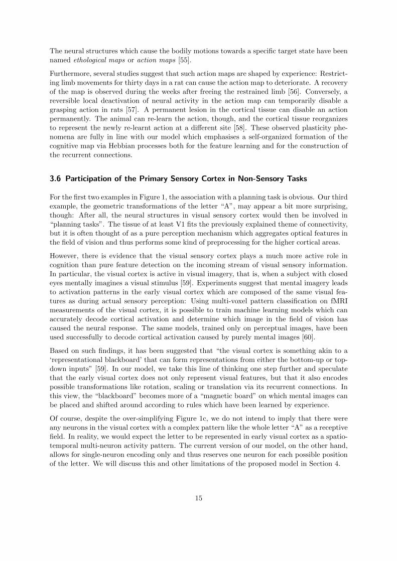
3.6 Participation of the Primary Sensory Cortex in Non-Sensory Tasks

For the first two examples in Figure 1, the association with a planning task is obvious. Our thirdexample, the geometric transformations of the letter “A”, may appear a bit more surprising,though: After all, the neural structures in visual sensory cortex would then be involved in“planning tasks”. The tissue of at least V1 fits the previously explained theme of connectivity,but it is often thought of as a pure perception mechanism which aggregates optical features inthe field of vision and thus performs some kind of preprocessing for the higher cortical areas.

However, there is evidence that the visual sensory cortex plays a much more active role incognition than pure feature detection on the incoming stream of visual sensory information.In particular, the visual cortex is active in visual imagery, that is, when a subject with closedeyes mentally imagines a visual stimulus [59]. Experiments suggest that mental imagery leadsto activation patterns in the early visual cortex which are composed of the same visual fea-tures as during actual sensory perception: Using multi-voxel pattern classification on fMRImeasurements of the visual cortex, it is possible to train machine learning models which canaccurately decode cortical activation and determine which image in the field of vision hascaused the neural response. The same models, trained only on perceptual images, have beenused successfully to decode cortical activation caused by purely mental images [60].

Based on such findings, it has been suggested that “the visual cortex is something akin to a‘representational blackboard’ that can form representations from either the bottom-up or top-down inputs” [59]. In our model, we take this line of thinking one step further and speculatethat the early visual cortex does not only represent visual features, but that it also encodespossible transformations like rotation, scaling or translation via its recurrent connections. Inthis view, the “blackboard” becomes more of a “magnetic board” on which mental images canbe placed and shifted around according to rules which have been learned by experience.

Of course, despite the over-simplifying Figure 1c, we do not intend to imply that there wereany neurons in the visual cortex with a complex pattern like the whole letter “A” as a receptivefield. In reality, we would expect the letter to be represented in early visual cortex as a spatio-temporal multi-neuron activity pattern. The current version of our model, on the other hand,allows for single-neuron encoding only and thus reserves one neuron for each possible positionof the letter. We will discuss this and other limitations of the proposed model in Section 4.

15

3.7 Temporal Dynamics

The concept presented in this article implies predictions about the temporal dynamics ofcognitive planning processes which can be compared to experiments: The bump of activityonly starts moving when the first wave front arrives. Assuming that every wave front has asimilar effect on the bump, its speed of movement should be proportional to the frequencywith which waves are emitted. Thus both the time until movement onset and the duration ofthe whole planning process should be proportional to the length of the traversed path in thecortical map. Increased frequency of wave emission should accelerate the process.

One supporting piece of evidence is provided by mental imagery: Experiments in the 1970s[61, 62] have triggered a series of studies on mental rotation tasks, where the time to compare arotated object with a template has often been found to increase proportionally with the angleof rotation required to align the two objects.

In the case of bodily motions, the total time to complete the cognitive task is not a well suitedmeasure since it strongly depends on mechanical properties of the limbs. Yet for electricalstimulation of the motor cortex (cf. Section 3.5) Graziano et al. report that the speed ofevoked arm movements increases with stimulation frequency [63]. Assuming that this frequencydetermines the rate at which the hypothetical waves of activation are emitted, this is consistentwith our model.

In addition, our model makes the specific prediction that the latency between stimulation andthe onset of muscle activation should increase with the distance between initial and targetposture. We are not aware of any studies having examined this particular relationship yet.

4 Discussion

The model proposed here is, to the best of our knowledge, the first model that allows for solvinggraph problems in a biological plausible way such that the solution (i. e. the specific path) canbe calculated directly on the neuronal network as the only computational substrate.

Similar approaches and models have been investigated earlier, especially in the field of neuro-morphic computing. For example, in [64–68] graphs are modeled using neurons and synapses,and computations are performed by exciting specific neurons which induces propagation ofcurrent in the graph and observing the spiking behavior. Although some models are moregeneral than the one presented here and allow for solving more complex problems like dynamicprograms [65], enumeration problems [67] or the longest shortest path problem [68], we arenot aware of any model explicitly discussing the biological plausibility. In fact, most of theseapproaches are far from being biologically plausible as they e. g. require additional artificialmemory [65] or a preprocessing step that changes the graph depending on the input data [68].Also, the model of Muller et al. [64] as well as the very recent model of Aimone et al. [66]which are biologically more plausible do not discuss how a specific path can then be computedin the graph, even if the length of a path can be calculated [66].

Our model has not been created with the intent to explain empirical findings from one par-ticular brain region, mental task or experimental technique in full detail. Rather, we sought

16

to explore ways in which a generic algorithmic framework might solve seemingly very differ-ent problems based on more or less the same neural substrate. Working on a relatively highlevel of abstraction and ignoring most of the domain-specific aspects may not only help ourunderstanding of computational principles employed by the brain but also pave the road to thedevelopment of new useful algorithms in artificial intelligence. Nevertheless, it is important tonote that many features of our model are in line with experimental results from various areasof brain science and we review those findings in Section 3.

In the following we discuss limitations of the presented model and potential avenues for furtherresearch.

4.1 Single-Neuron vs. Multi-Neuron Encoding

In our model, each point on a cortical map is represented by a single neuron and a distance onthe map is directly encoded in a synaptic strength between two neurons. The graph of synapticconnections an therefore be considered as a coarse-grained version of the underlying manifoldof stimuli. Yet such a single-neuron representation is possible only for manifolds of a very lowdimension, since the number of points necessary to represent the manifold grows exponentiallywith each additional dimension. For tasks like bodily movement, where dozens of joints needto be coordinated, the number of neurons required to represent every possible posture in asingle-neuron encoding is prohibitive. Therefore, it is desirable to encode manifolds of stimuliin a more economical way – for example, by representing each point of the manifold by acertain set of neurons. It is an open question how distance relationships between such groupsof neurons could be encoded and whether the dynamics from our model could be replicated insuch a scenario.

4.2 Wave Propagation and Continuous Attractor Layers

Certain design choices made in the numerical implementation should be discussed regardingtheir biological plausibility and possible alternative mechanisms.

If the wave propagation layer and the continuous attractor layer were to form organically as twoseparate sub-circuits in a real biological system, each of their neurons would need to act as afeature detector, since otherwise it is not clear how the right structure of recurrent connectionscould develop. Then each feature will be represented by two detectors – one in each layer –and there must be some unknown mechanism which establishes a link between every pair ofcorresponding feature detectors.

Moreover, the split of the model dynamics into two layers leads to a somewhat artificial im-plementation of the interaction between them: As described in Section 2.4, we compute thedirection into which the activation bump in the continuous attractor layer is shifted whenevera wave front arrives at the corresponding location in the wave propagation layer. The details ofthis mechanism do not appear to be biologically plausible and we would rather expect that thebump is moved only by the aggregated effects of local interactions between synaptically con-nected neurons. This interaction could be mediated by the connections between correspondingfeature detectors which we postulated above.

17

Alternatively, an elegant and biologically plausible model could be obtained by merging thewave propagation and continuous attractor dynamics into a single layer of neurons. In such asingle-layer model, the whole network can form in a self-organized way: First, the feed-forwardconnections are generated via a process of competitive Hebbian learning, leading to a networkof individual feature detectors. In a second step, these detectors establish recurrent connectionsamong each other, again driven by Hebbian learning, to create the graph structure required inour model.

In the single-layer scenario, the model must allow for continuous attractor dynamics and wave-like expansion of activity simultaneously. We speculate that this is possible in principle, forexample by imposing a time delay on the effect of inhibition – which appears biologicallyplausible considering that it is mediated in an extra step via inhibitory interneurons. Thetime delay of inhibition has only minimal effect on the quasi-static peak of activity and thusconserves the landscape of continuous attractors from the two-layer scenario. On the otherhand, the time delay allows activation patterns with strong temporal fluctuations to emit wavesof activity before inhibition has any effect.

The interaction between the waves and the localized peak of activity could potentially shiftthe peak in the direction of the incoming waves without the need to impose any artificialassumptions to the model: The incoming waves are annihilated by the peak’s “trench ofinhibition”, but they also increase the level of activation of the neurons on the side of thebump which is hit by the wave. Due to the attractor dynamics of the network the bumprecovers from this deformation, but in the process it changes its location slightly towards thedirection of the incoming wave.

Realizing the effects described above will require a very careful numerical set-up of the modeland tuning of its parameters. We consider this an interesting direction for future research sincethe potential outcome is a rather elegant model with a high degree of biological plausibility.

4.3 Embedding into a Bigger Picture

While the model focuses on the solution of graph traversal problems, it appears desirable toembed it into a broader context of sensory perception, decision making, and motion controlin the brain. One particular question is how the hypothetical “puppet string mechanism” –which we postulated to connect proprioception and motion control – could be implemented ina neural substrate. Similarly, if our model provides an appropriate description of place cellsand their role in navigation, the question arises how a shift in place cell activity is translatedinto appropriate muscle commands to propel the animal in the corresponding direction.

It is intriguing to speculate about a deeper connection between our model and object recog-nition: On the same neural substrate, our hypothetical waves might travel through a space ofpossible transformations, starting from a perceived stimulus and “searching” for a previouslylearned representative of the same class of objects. This could explain why recognition ofrotated objects is much faster than the corresponding mental rotation task [69]: The formerwould require only one wave to travel through the cognitive map, while the later would requiremany waves to move the bump of activity.

18

And finally, an open question is the connection between the model and the hypothetical ex-ecutive brain functions which are assumed to define the target state for the graph traversalproblem and activate the corresponding neurons.

5 Conclusion

We have shown that a wide range of cognitive tasks, especially those that involve planning,can be represented as graph problems. To this end, we have detailed one possible role for therecurrent connections that exist throughout the brain as computational substrate for solvinggraph traversal problems. We showed in which way such problems can be modeled as findinga short path from a start node to some target node in a graph that maps to a manifoldrepresenting a relevant task space. Our review of empirical evidence indicates that a theme ofconnectivity can be observed in the neural structure throughout (at least) the neocortex whichis well suited to realize the proposed model.

We constructed a two-layer neural network consisting of a layer of neurons that implementeda continuous attractor sheet modelled after neurons found in the human hippocampus andenthorinal cortex. This sheet of neurons enacts a ”bump” of activity centered on the neuronrepresenting the start node s in the graph. As a second step we implemented a sheet of spikingneurons that generated a wave of activation across the same sheet starting from a individualneuron that represented the target node t in the graph. Finally, we implemented an interactionalgorithm which caused the bump of activation in the continuous attractor layer to move inthe direction of the wave front as it reached the region of activation in the continuous attractorlayer. We found that this model was successfully able to move the activation bump in thecontinuous attractor layer through the sheet of neurons to the location that mapped to thetarget node t in the graph, thus solving the graph traversal problem. We found further thatthe model was robust to large changes in the graph structure. Specifically we showed that iflarge portions of the graph are made inaccessible and the relevant neurons in the model werezeroed out that the model is still able to guide the activation bump from the start node s tothe target node t successfully.

Despite its relatively small scale we believe that models such as ours may provide a startingpoint in understanding how brains are able to exhibit flexible behaviour with respect to differentkinds of cognitive tasks. Apparently, the stereotypical theme of connectivity encountered acrossthe neocortex allows the brain to create a model of its environment based on sensory perception.Once established, the neural structure can be used as a “planning board” to support differentcognitive tasks.

Next to a deeper understanding of the brain, we believe that models like ours can be aninspiration for new algorithms of artificial intelligence (AI). Artificial neural networks used intechnical applications today are typically input-driven, they rely on feed-forward processing ofinformation through several layers of neurons, and they are trained via supervised learning. Thebrain, however, continuously integrates sensory input into its own dynamics, its connectivitystructure is mostly recurrent, and learning happens to a large extent in an unsupervised way.In all three of these fundamental differences, our model is aligned more closely to the propertiesof the brain than those of most other AI algorithms. At the same time, it shows how relevant

19

computational problems can be solved with a very generic approach that relies heavily on self-organization. Potential applications include motion control for robots, especially in scenarioswhich require a high degree of flexibility and continuous adaptation to changing circumstances.As an additional interesting feature, since the model is based on artificial spiking neurons, itcan potentially be implemented very efficiently in neuromorphic computer hardware.

Acknowledgements

The authors gratefully acknowledge funding from the European Research Council (ERC) un-der the European Union’s Horizon 2020 research and innovation program (Grant agreement677270) which allowed H. P. to undertake the work described in the above. We also thankRaul Mures,an and Robert Klassert for providing very valuable comments on early drafts ofthe paper.

Methods and Experiments

Connection to Mathematical Graph Traversal Problems

As the model described in Section 2 uses a neural network of neurons to solve planning problemsin the cognitive map, it is natural to interpret this network as a graph consisting of nodesrepresenting the neurons and edges representing their synaptic connections. Thus, the planningproblem in the network translates into a graph traversal problem in the corresponding graph.In the following, we hence introduce some basic terminology used in the field of graph theory.

We refrain from giving too many details and references, as most of the standard formalism canbe found in classical books on mathematical optimization. In particular, we refer to [70, 71]for references, details, proofs and further discussions.

A graph G is a pair G = (V, E), where V is a finite set of nodes and E is the set of edges,where each edge is set of two nodes. For two nodes s, t ∈ V, an s-t-path is a path of nodesstarting at s and ending at the target node t such that any two consecutive nodes along thepath are connected by an edge. A node t ∈ V is reachable from another node s ∈ V if thereexists an s-t-path in G. An example of a graph with 15 nodes and different paths is given inFigure 6.

20

ab c d

e

f g

h

i j

kl

mn

o

Figure 6: An example of a graph G with 15 nodes. The red resp. blue edges show two a-o-pathsin the graph.

In the following, we let G = (V, E) be a fixed graph. For simplicity, we assume that every nodeis reachable from every node.

We are interested in finding a path between two given nodes s, t ∈ V in G. The idea is that thenode t represents the neuron encoding the to-be state and s represents the neuron encodingthe as-is state of the underlying planning problem. To formalize this problem, we denote byPath(s, t) the problem of finding a path from s to t for given nodes s, t.

Even though this problem technically only asks for finding some path from s to t, shorter pathsthat use as few connections as possible are superior to longer paths using more connections.The reason is that the fewer connections a path has, the fewer intermediate states are traversedin the planning problem. When considering the previous example of grabbing a cup of coffee,a possible solution could be to move the arm around the head before performing actuallyreaching towards the coffee cup. This is not the movement that would be performed in actualbehavior. However, we are similarly not obliged to find the shortest possible path. Consideringthe previous example again, a shortest path would reflect a movement with as few intermediatepositions as possible. This might correspond to stretching the arm in such a way that the cupcan barely be reached and might yield an unrealistic behavior. Thus, in summary, our goal isto find reasonably short paths that do not necessarily need to be shortest paths.

The Path(s, t) problem is a well-investigated problem in computer science and mathematics.With BFSand DFS, two standard path finding algorithms from computer science are describedin Section 5. There, we also argue why these approaches cannot directly be applied to our sce-nario due to the fact that the graphs we consider represent neural networks in which algorithmshave to be performed in a biological plausible way.

Mathematical Background and Solving the Path Problem in Typical Graphs

In the following, we consider how the Path(s, t) problem can be solved in general graphs thatdo not represent neural networks. We later discuss what problems occur when trying to adaptthese algorithms to such graphs when using the neurons as computational substrate. In all ofthe following, we omit technical details and proofs and instead refer to [70, 71] again.

Consider some fixed graph G = (V, E) and two nodes s, t ∈ V. For simplicity, we assume thatthere is at least one path between any pair of nodes. The most basic class of algorithms that

21

can be used to solve the Path(s, t) problem is the class of graph search algorithms. Two ofthe most prominent examples of graph search algorithms are Breadth-First-Search (BFS ) andDepth-First-Search (DFS ).

Both algorithms start at the starting node s and traverse the graph iteratively by following itsedges. Intuitively, DFS (s) tries to follow a single path starting in s for as long as possible, onlyreturning to a previously considered node and starting a “new” path if it is strictly necessary.In contrast to this, BFS (s) tries to always visit a node as close as possible to the startingnode s next. A visualization of the results of these two algorithms applied to the same graphstarting at node a is given in Figure 7. By remembering which nodes are already completelyexplored, both of these algorithms find all nodes reachable from the starting node s.

ab c d

e

f g

h

i j

kl

mn

o

ab c d

e

f g

h

i j

kl

mn

o

Figure 7: Exemplary result of BFS (a) (left) and DFS (a) (right). Each node but a points toits parent node.

In particular, the algorithms are typically implemented in a way that the traversed paths caneasily be recovered from the data produced by the algorithms. As both algorithms are verysimilar, they can be implemented as a realization of a general scheme for finding paths in agraph. This scheme is given in Algorithm 1. It uses a generic data structure D that onlyhas to allow for the two basic operations of inserting in and removing nodes from it. In eachstep, the algorithm extracts a node u from D and checks for unvisited nodes among all nodeswhich have an edge towards u. For each such node w, the algorithm inserts w into the datastructure D and remembers that the node w was reached from u by marking u as the parentof w. To avoid visiting vertices more than once, the node w is then also marked as visited.After performing this step for each such node, the node u is completely explored and it is notnecessary to consider it again.

Depending on the specific data structure that is chosen for D, this then yields either the BFSorthe DFS algorithm. More precisely, if D is chosen as a queue that inserts and removes nodes

22

first-in-first-out, then Algorithm 1 yields the BFSalgorithm. If D is chosen as a stack thatinserts and removes nodes last-in-first-out, then one obtains the DFS algorithm.

Data: graph G = (V, E). node s ∈ V

Result: calculated parent p(w) for each w ∈ V

1 D := (s)

2 p(s) := s

3 Mark s as visited

4 while D 6= ∅ do5 u := ExtractElement(D)

6 foreach w that has an edge to u do7 if w is not marked as visited then8 Insert w into D

9 p(w) := u

10 Mark w as visited

11 return list of parents p

Algorithm 1: The generic graph traversal algorithm. Choosing a queue for D yieldsthe BFSalgorithm, choosing a stack yields the DFS algorithm.

Both variants of this algorithmic scheme can solve the Path(s, t) problem. However, as men-tioned in Section 2, we want to find a short path from s to t. This is guaranteed if we use theBFS (s) algorithm as this algorithm always finds shortest paths with respect to the numberof edges. We later argue why this result implies that we are able to find short paths in theneural network representing the manifold of stimuli, even if we cannot guarantee that they areshortest paths.

We now discuss why it is not biologically plausible that graph traversal problems in the brainare solved by exactly one of these algorithms. The main obstacle is that Algorithm 1 requiresthe data structure D to organize the nodes that still have to be considered, as well as amechanism to remember which nodes have already been visited. Especially the data structureD which might have to store a large number of nodes and is in some sense “global” cannotbe implemented in the brain in a way it can be implemented in a computer. The reason isthat individual neurons in a neural network can only access local information or informationthat was just sent to them by a pre-synaptic neuron. In a neural network, however, neuronsare only able to communicate with their synaptic neighbors via sending and receiving electriccurrent.

As discussed in Section 2.6, our network configuration yields a wave propagation that behaveslike a “parallelized” version of BFSwhere a set of nodes can be visited simultaneously. Thisalso explains how using a wave propagation algorithm can find short paths, but not necessarilyshortest paths: A neuron potentially receives current from more than one neuron, hence it isnot possible to uniquely retrace the path to the starting node. However, as wave propagationbehaves like a parallelized BFSalgorithm, the paths that can be obtained via backtracking willnever be too long. Although this behavior has some similarities with other well-understood

23

graph problems like virus propagation [72–74] or diffusion processes [75] in networks, therespective theories are not directly applicable to our specific scenario.

Neuronal Network Setup – Exemplary Implementation of the Model

Splitting Dynamics to Two Network Layers As described in Section 2.2, for our numericalimplementation of the model, we separated the two different types of dynamics into distinctlayers of neurons, the continuous attractor layer and the wave propagation layer. The splitinto two layers makes the model more transparent and ensures that parameter changes havelimited and traceable effects on the over-all dynamics. As an additional simplification, we donot explicitly model the feed-forward connections which drive the wave propagation layer, butwe rather directly activate certain neurons in this layer.

Activation in the continuous attractor layer C represents the start node s, that in the courseof the simulation will move towards the target node t, which is permanently stimulated in thewave propagation layer P . Waves of activation are travelling from t across P . As soon asthe wave front reaches a node in P that is connected to a node in proximity to the currentactivation in C, the activation in C is moved towards it. Thus, every arriving wave front willpull the activation in C closer to t, forcing the activation to trace back the wave propagationto its origin t.

In detail, these dynamics require a very specific network configuration which is described inthe following. Figure 8 contains a general overview of the intra- and inter-layer connectivityused in the model and our simulations.

Spiking Neuron Model in the Wave Propagation Layer In the performed experiments, thewave propagation layer P is constructed with an identical number of excitatory and inhibitoryIzhikevich neurons [14, 15], that cover a regular quadratic grid of 41×41 points on the manifoldof stimuli. The spiking behavior of each artificial neuron is modeled as a function of itsmembrane potential dynamics v(t) using the two coupled ordinary differential equations

d

dtv = 0.04v2 + 5v + 140− u+ I, (1)

d

dtu = a · (bv − u). (2)

Here, v is the membrane potential in mV, u an internal recovery variable, and I representssynaptic or DC input current. The internal parameters a (scale of u / recovery speed) andb (sensitivity of u to fluctuations in v) are dimensionless. Time t is measured in ms. If themembrane potential grows beyond the threshold parameter v ≥ 30 mV, the neuron is spikingand the variables are reset as follows.

v ← c, (3)

u← u+ d. (4)

Again, c (after-spike reset value of v) and d (after-spike offset value of u) are dimensionlessinternal parameters.

24

place cell bump

pt mean (At)

∆(t)

Continuous attractor layer C

Wave propagation layer P

inhibitoryneurons

excitatoryneurons

0s(max)e→ed

0 s(max)e→ids

(max)i→ed

s(max)i→e

inhib. range diinhib. range di

excitation range deexcitation range de

Grid step δ widthd = n · δ, n ∈ N (in 1D)

Figure 8: Connectivity of the neurons. For simplicity, this visualization only contains a 1Drepresentation. In the wave propagation layer, excitatory synapses are drawn assolid arrows, dashed arrows indicate inhibitory synapses. Upon its activation, thecentral excitatory neuron stimulates a ring of inhibitory neurons that in turn suppresscircles of excitatory neurons to prevent an avalanche of activation and support acircular wave-like expansion of the activation across the sheet of excitatory neurons.Furthermore, overlap between the active neurons in C and P is used to compute thedirection vector ∆(t) used for biasing synapses in C and thus shifting activity there.

If not stated otherwise in the following, the parameters listed in Table 1a were used for thespiking neuron model in P . They correspond to regular spiking (RS) excitatory and fastspiking (FS) inhibitory neurons. In contrast to [14], neuron properties were not randomizedto allow for reproducible analyses. The effect of a more biologically plausible heterogeneousneuron property and synaptic strength distribution is analyzed in Section 5. Compared to [14],the coupling strength in P is large to account for the extremely sparse adjacency matrix asevery neuron is only connected to its few proximal neighbours in our configuration. Whenevera neuron in P is to be stimulated externally, a DC current of I = 25 is applied to it, cf.Equation (1). As in [14], the simulation time step was fixed to 1 ms with one sub-step in P fornumerical stability.

Synaptic Connections in the Wave Propagation Layer As described before, neurons in Pcorrespond to reachable locations in the manifold of stimuli. Thus, it is plausible to assumethat neurons representing near-by locations in a suitable metric on the respective manifold willalso be closely connected. Assuming that neurons will not have a very strictly defined regionof responsibility, but there will also be some overlap, this is consistent with a Hebbian learning

25

excitatory inhibitoryRS FS

a 0.02 0.1b 0.2 0.2c −65 −65d 8 2

(a) Neuron model parameters(homogeneous setup).

excitatory inhibitoryRS . . . CH LTS . . . FS

a 0.02 0.02 + 0.08rib 0.2 0.25− 0.05ric −65 + 15r2e -65d 8− 6r2e 2

(b) Neuron model parameters(heterogeneous setup).

s(max)e→e 50

s(max)e→i 0.5 s

(max)e→e

s(max)i→e −9 s

(max)e→e

de 2

(c) Synaptic strengthparameters.

Table 1: Parameters used in our simulations of the wave propagation layer P .

approach: Neurons that are sensitive to nearby regions will often fire at the same instant intime, strengthening their mutual connectivity.

As depicted in Figure 8, the excitatory neurons are driving nearby excitatory and inhibitoryneurons with a synaptic strength of

se→e(d) :=

s(max)e→e

d, for 0 < d ≤ de

0, else

, (5)

where se→i(d) is defined analogously. Here, d is the distance between nodes in the manifoldof stimuli. For simplicity, we model this manifold as a two-dimensional quadratic mesh withgrid spacing δ = 1 where some connections might be missing. The choice s ∝ 1/d was made torepresent the assumption that recurrent coupling will be strongest to nearest neighbours andwill decay with distance. Note that (5) in particular implies that we have se→e(0), se→i(0) = 0,which prevents self-excitation. To restrict to only localized interaction, we exclude interactionbeyond a predefined excitation range de and inhibition range di, respectively. Values of theparameters in the expressions for the synaptic strengths used in the simulations are given inTable 1c.

The inhibitory neurons suppress activation of the excitatory neurons by reducing their inputcurrent via synaptic strength

si→e(d) :=

s(max)i→e , for d = 0

s(max)i→e

d, for 0 < d ≤ ds

0, else

. (6)

Wave Propagation Dynamics The described setup allows for wave-like expansion of neuronalactivity from an externally driven excitatory neuron as shown in Figure 9.

If the activity of the excitatory neurons grows too much in a region, the respective inhibitoryneurons will start spiking to eventually suppress activity locally. This suppression happenswith a delay of two time steps due to the causal signal travelling time through se→e and se→i,

26

Excitatory Firing Pattern Inhibitory Firing Pattern

Figure 9: Activity patterns of the excitatory and inhibitory neurons on a 101× 101 quadraticneuron grid. Spiking neurons are shown as gray areas. One excitatory neuron at thegrid center (arrow) is driven by an external DC current to regular spiking activity.Due to the nearest-neighbour connections, this activity is propagating in patternsthat resemble a circular wave structure. The inhibitory neurons prevent catastrophicavalanche-like dynamics by suppressing highly active regions. The specific patternshape is an artifact of the underlying regular grid structure and thus not perfectlycircular. This could be alleviated using, e. g. a hexagonal instead of a quadraticmesh of neurons.

but could also be implemented via different synaptic time constants, i. e. AMPA (excitatory)vs. GABA A (inhibitory). Thus, the inhibitory neurons prevent an avalanche-like activity byturning off active excitatory neurons.

As can be seen in Figure 9, this effectively means that propagating signals in the excitatory sub-network are followed by similarly shaped propagating signals in the inhibitory sub-network. Inthis respect, signal propagation does not behave like physical waves, such as ripples on water:They do not interfere in constructive and destructive manner to form interference patterns.Instead, activity stops where to propagating signals touch as shown in Figure 10. This is animportant property in our setup as it ensures that signals do not run through each other inthe wave propagation layer but do mutually annihilate. Thus, the wave fronts tend to formstable and continuous patterns and activation of the continuous attractor layer from differentdirections is vastly reduced.

27

t = 10ms t = 15ms t = 18ms

Figure 10: Activity patterns of the excitatory neuron grid where two neurons are driven toperiodic spiking activity (arrows) at different instants in time. Again, spiking neu-rons are shown as gray areas and neuronal connections are set up as described inSection 5 As soon as the signal propagation fronts touch, they annihilate each otherdue to the inhibitory activity that accompanies them. Instead of forming interfer-ence patterns or travelling through each other, the remaining wave fronts mergeand continue propagating as a well-defined line of activity.

With the capability of propagating signals as circular waves from the target neuron t acrossthe manifold of stimuli in P , it is now necessary to set up a representation of the start neuron sin C. This will be done in the following subsection before the coupling between P and C willbe described.

Neuron Model for Place Cell Dynamics The continuous attractor layer C, implements asheet of neurons that models the functionality of a network of place cells in the human hip-pocampus using rate-coding neurons [11, 12] and thus the manifold of stimuli. As for the wavepropagation layer, we also use a quadratic 41 × 41 grid of neurons for this layer. Activationin the continuous attractor layer will appear as bump, the center of which represents the mostlikely current location on the manifold of stimuli.

This bump of activation is used to represent the current position in the graph of synapticconnections representing the cognitive map. Planning in the manifold of stimuli thus amountsto moving the bump through the sheet of neurons where each neuron can be thought of asone node in this graph. With respect e. g. to the robot arm example in Figure 1b, the placecell bump represents the current state of the system i. e. the current angles of the arm’s twodegrees-of-freedom. As the bump moves through the continuous attractor layer, and thusthrough the graph, the robot arm will alter its configuration creating a movement trajectorythrough the 2D space.

Synaptic Connectivity to Realize Continuous Attractor Dynamics Our methodology formodelling the continuous attractor place cell dynamics adapts the computational approach usedin [13] by including a computational consideration for synaptic connections between continuousattractor neurons and an associated update rule that depends on information from the wavepropagation layer P .

28

σ Gaussian width 0.03T Gaussian shift 0.05J Synaptic connection strength 12τ Stabilization strength 0.8

Table 2: Parameters for the continuous attractor layer C.

The synaptic weight function connecting each neuron in the continuous attractor sheet to eachother neuron is given by a weighted Gaussian. This allows for the degrading activation ofcells in the immediate neighbourhood of a given neuron and the simultaneous inhibition ofneurons that are further away, thus giving rise to the bump-shaped activity in the sheet itself.The mathematical implementation of these synaptic connections also allows for the locus ofactivation in the sheet to be shifted in a given direction which is, in turn, how the graphimplemented by this neuron sheet is able to be traversed.

The synaptic weight w~i,~j ∈ R(Nx×Ny)×(Nx×Ny) connecting a neuron at position ~i = (ix, iy) to a

neuron at position ~j = (jx, jy) is given by

w~i,~j := J · exp

(− 1

σ2

∥∥∥∥( ix − jxNx,iy − jyNy

)+ ~∆(t)

∥∥∥∥2)− T . (7)

Here, J determines the strength of the synaptic connections, ‖·‖ is the Euclidean norm, σmodulates the width of the Gaussian, T shifts the Gaussian by a fixed amount, ~∆(t) is adirection vector which we discuss in detail later, and Nx and Ny give the size of the twodimensions of the sheet.

In order to update the activation of the continuous attractor neurons and to subsequentlymove the bump of activation across the neuron sheet, we compute the activation A~j of the

continuous attractor neuron ~j at time t+ 1 using

B~j(t+ 1) =∑~i

A~i(t)w~i,~j(t) , (8)

A~j(t+ 1) = (1− τ)B~j(t+ 1) + τB~j(t+ 1)∑

~iA~i(t), (9)

where B~j(t+ 1) is a transfer function that accumulates the incoming current from all neurons

to neuron ~j and τ is a fixed parameter that determines stabilization towards a floating averageactivity.

Simulation parameters for the continuous attractor layer C are given in Table 2. They havebeen manually tuned to ensure development of stable, Gaussian shaped activity with an effec-tive diameter of approximately twelve neurons in C.

As in [13], a direction vector ~∆(t) ∈ R2 has been introduced in Equation (7). It has the effectof shifting the synaptic weights in a particular direction which in turn causes the location ofthe activation bump in the attractor layer to shift to a neighbouring neuron. In other words, itis this direction vector that allows the graph to be traversed by informing the place cell sheetfrom which direction the wave front is coming in P . Thus all that remains for the completion

29

of the necessary computations is to compute ~∆(t) as a function of the propagating wave andthe continuous attractor position.

Layer Interaction - Direction Vector The interaction between the wave propagation layer Pand the continuous attractor layer C is mediated via the direction vector ~∆(t). The directionvector is computed such that it points from the center of the bump of activity towards thecenter of the overlap between bump and incoming wave as follows. Let Ct and Pt denote thesets of positions of active neurons at time t in layer C and P , respectively. Note that eachpossible position corresponds to exactly one neuron in the wave propagation layer and exactlyone neuron in the continuous attractor layer as they have the same spatial resolution in theimplementation. Now let At := Ct ∩ Pt. Then,

mean (At) =1

|At|∑~i∈At

~i (10)

is the average position of overlap. We compute the direction vector from the current positionpt of the central neuron in the continuous attractor layer activation bump to mean (At) via

~∆(t) = mean (At)− pt . (11)

Layer Interaction - Recovery Period In order to prevent the wave from interacting with theback side of the bump in C, we introduce a recovery period R of a few time steps after movingthe bump. During R, which is selected as the ratio of bump size to wave propagation speed,At is assumed to be empty, which prevents any further movement. In our experiments, weused R = 12 ms.

It is worth acknowledging at this point that this approach of connecting the two layers, whichwe have chosen for reasons of simplicity, is somewhat artificial. We discuss this and otherlimitations of our implementation in Section 4.2.

Numerical Experiments

In order to test the complex neuronal network configuration described in Sections 2 and 5and to study its properties and dynamics, we performed numerical experiments using multipledifferent setups. Source code used for our studies is published at [76]. Results of our simulationsare presented in Section 2.5. In the following, we will add some more in-depth analyses onspecific properties of the model as observed in the simulations.

Transmission Velocity In our setup, no synaptic transmission delay, as e. g. in [77], is imple-mented. As, due to the strong nearest-neighbour connectivity, only few pre-synaptic spikingneurons are sufficient to raise the membrane potential above threshold, the waves are travel-ling across P with a velocity of approximately one neuronal “ring” per time step, cf. Figure 4.In contrast, the continuous attractor can only move a distance of at most half its width perincoming wave. Accordingly, its velocity is tightly coupled to the spike frequency of the stim-ulated neuron while still being bound due to the recovery period R. In the specific case of the

30

simulation in Figure 4, in total nine wave fronts were observed to be required traversing theGaussian continuous attractor activity zone to finally pull it on a straight line to its destinationover a distance of d = 45.25.

Obstacles and Complex Setups In the S-shaped maze Figure 5a, the continuous attractoractivity moves towards the target node t on a direct path around the obstacles. Due to theoptimal path being more than two times longer than in Figure 4, the time to reach the targetis accordingly longer as well. This is also in line with the required travel times from s to t inFigures 5b and 5c, where – despite its complexity – a path through the maze is found fastestdue to it being shorter than in the other cases of Figure 5. This observation is also evidencedby the fact that our model is a parallelized version of BFS, cf. Sections 2.6 and 5, which isguaranteed to find the shortest path in an unweighted and undirected graph.

Symmetric Paths An additional interesting observation can be made in the central blocksetup, Figure 5b: The setup is perfectly symmetric with respect to the two possible paths.Thus, in principle it can not be solved with our model. However, after interaction with sev-eral wave fronts, a minor shift of the continuous attractor position occurs due to numericalinstability. This is further emphasized by subsequent incoming waves, finally pulling the con-tinuous attractor onto a path to the target node t. While such numerical instabilities areclearly resulting from the specific implementation of our model on a computer system, alsoorganically grown biologic networks will never be perfectly symmetric. Here, natural variationsin synaptic connectivity and neuron properties will break potential symmetries, favoring one ofthe possible paths. In the following, we inspect the influence of these variations on the overallperformance of the model.

Heterogeneous Neuron Properties and Synaptic Strengths In the simulation experimentsdescribed up to now, a homogeneous wave propagation layer P is employed. There, all neuronsare subject to the same internal parameters, being either regular spiking excitatory neurons orfast spiking inhibitory neurons. Also, synaptic strengths are strictly set as described previouslywith parameters from Table 1c. This setup is rather artificial. Natural neuronal networks willexhibit a broad variability in neuron properties and in the strength of synaptic connectivity.

To account for this natural variability, we randomized the individual neuron’s internal prop-erties as suggested in [14], see Table 1b. As in [14], heterogeneity is achieved by randomizingneuron model parameters using random variables re and ri for each excitatory and inhibitoryneuron. These are equally distributed in the interval [0; 1] and vary neuron models betweenregular spiking (re = 0) and chattering (CH, re = 1) or fast spiking (ri = 1) for excitatoryneurons and low-threshold spiking (LTS, ri = 0) for inhibitory neurons. By squaring re, excita-tory neuron distribution is biased towards RS. In addition, after initializing synaptic strengthsin P , we randomly varied them individually by up to ±50 %.

Despite this strong modification to the original numerically ideal setup, a structured wavepropagation is still possible in P as can be seen in Figure 11. While the stereotypical circularform of the wave fronts dissolves in the simulation, they continue to traverse P completely.As before, they reach the continuous attractor bump and are able to guide it to their origin.

31

t = 25ms t = 175ms t = 325ms t = 365ms t = 375ms t = 430ms

Figure 11: Block setup as in Figure 5 but with a heterogeneous neuron configuration in P .

Apparently, the overall connection scheme in P is more important for stable wave propagationthan homogeneity in the individual synaptic strengths and neuron properties.

An interesting aspect of this simulation when compared to Figure 5b is the apparent capabilityof solving the graph traversal problem quicker than with the homogeneous neuronal network.As already indicated, this is an artifact of the explicitly broken symmetry in the heterogeneousconfiguration: The wave fronts from different directions differ in shape when arriving at theinitial position of the continuous attractor layer activity. Thus, one of them is immediatelypreferred and target-oriented movement of the bump starts earlier than before. This capabilityof breaking symmetries and thus quickly resolving ambiguous situations is an explicit advantageof the more biologically realistic heterogeneous configuration.

References

[1] R. J. Douglas and K. A. Martin. “Recurrent neuronal circuits in the neocortex”. In:Current Biology 17.13 (2007), R496–R500. doi: 10.1016/j.cub.2007.04.024.

[2] W. Singer and A. Lazar. “Does the Cerebral Cortex Exploit High-Dimensional, Non-linear Dynamics for Information Processing?” In: Frontiers in Computational Neuro-science 10 (2016). doi: 10.3389/fncom.2016.00099.

[3] E. K. Miller and T. J. Buschman. “Cortical circuits for the control of attention”. In:Current Opinion in Neurobiology 23.2 (2013), pp. 216–222. doi: 10.1016/j.conb.2012.11.011.

[4] K. Kveraga, A. S. Ghuman, and M. Bar. “Top-down predictions in the cognitive brain”.In: Brain and Cognition 65.2 (2007), pp. 145–168. doi: 10.1016/j.bandc.2007.06.007.

[5] D. E. Rumelhart and D. Zipser. “Feature Discovery by Competitive Learning”. In: Cog-nitive Science 9.1 (1985), pp. 75–112. doi: 10.1207/s15516709cog0901_5.

[6] T. Kohonen. “Self-organized formation of topologically correct feature maps”. In: Bio-logical Cybernetics 43.1 (1982), pp. 59–69. doi: 10.1007/BF00337288.

[7] T. Martinetz and K. Schulten. “Topology representing networks”. In: Neural Networks7.3 (1994), pp. 507–522. doi: 10.1016/0893-6080(94)90109-0.

[8] M. Elad. Sparse and Redundant Representations. Springer, 2010.

[9] C. Curto and V. Itskov. “Cell Groups Reveal Structure of Stimulus Space”. In: PLoSComputational Biology 4.10 (2008). Ed. by K. J. Friston, e1000205. doi: 10.1371/

journal.pcbi.1000205.

32

[10] E. T. Rolls. “Attractor networks”. In: WIREs Cognitive Science 1.1 (2010), pp. 119–134.doi: 10.1002/wcs.1.

[11] J. O’Keefe and J. Dostrovsky. “The hippocampus as a spatial map. Preliminary evidencefrom unit activity in the freely-moving rat”. In: Brain Research 34.1 (1971), pp. 171–175.doi: 10.1016/0006-8993(71)90358-1.

[12] J. O’Keefe. “Place units in the hippocampus of the freely moving rat”. In: ExperimentalNeurology 51.1 (1976), pp. 78–109. doi: 10.1016/0014-4886(76)90055-8.

[13] A. Guanella, D. Kiper, and P. Verschure. “A model of grid cells based on a twistedtorus topology”. In: International journal of neural systems 17 (2007), pp. 231–40. doi:10.1142/S0129065707001093.

[14] E. M. Izhikevich. “Simple model of spiking neurons”. In: IEEE Transactions on NeuralNetworks 14.6 (2003), pp. 1569–1572. doi: 10.1109/TNN.2003.820440.

[15] E. M. Izhikevich. “Which model to use for cortical spiking neurons?” In: IEEE Transac-tions on Neural Networks 15.5 (2004), pp. 1063–1070. doi: 10.1109/TNN.2004.832719.

[16] E. C. Tolman and C. H. Honzik. Introduction and removal of reward and maze perfor-mance in rats. University of California publications in psychology v. 4, no. 17. Universityof California Press, 1930.

[17] E. C. Tolman. “Cognitive Maps in Rats and Men”. In: Psychological Review 55.4 (1948),pp. 189–208. doi: 10.1037/h0061626.

[18] J. O’Keefe and L. Nadel. The Hippocampus as a Cognitive Map. Oxford: Clarendon Press,1978. doi: 10.1016/j.neuron.2015.06.013.

[19] D. Bush et al. “Using Grid Cells for Navigation”. In: Neuron 87.3 (2015), pp. 507–520.doi: 10.1016/j.neuron.2015.07.006.

[20] T. Hafting et al. “Microstructure of a spatial map in the entorhinal cortex”. In: Nature436 (2005), pp. 801–6. doi: 10.1038/nature03721.

[21] J. Taube, R. Muller, and J. Ranck. “Head-direction cells recorded from the postsubiculumin freely moving rats. I. Description and quantitative analysis”. In: Journal of Neuro-science 10.2 (1990), pp. 420–435. doi: 10.1523/JNEUROSCI.10-02-00420.1990.

[22] J. L. Gauthier and D. W. Tank. “A Dedicated Population for Reward Coding in theHippocampus”. In: Neuron 99.1 (2018), 179–193.e7. doi: 10.1016/j.neuron.2018.06.008.

[23] A. O. Constantinescu, J. X. O’Reilly, and T. E. J. Behrens. “Organizing conceptualknowledge in humans with a gridlike code”. In: Science 352.6292 (2016), pp. 1464–1468.doi: 10.1126/science.aaf0941.

[24] C. Doeller, C. Barry, and N. Burgess. “Evidence for grid cells in a human memorynetwork”. In: Nature 463 (2010), pp. 657–61. doi: 10.1038/nature08704.

[25] K. Cameron et al. “Human Hippocampal Neurons Predict How Well Word Pairs Will BeRemembered”. In: Neuron 30 (2001), pp. 289–98. doi: 10.1016/S0896-6273(01)00280-X.

33

[26] P. Alvarez, L. Wendelken, and H. Eichenbaum. “Hippocampal Formation Lesions ImpairPerformance in an Odor-Odor Association Task Independently of Spatial Context”. In:Neurobiology of Learning and Memory 78 (2002), pp. 470–476. doi: 10.1006/nlme.2002.4068.

[27] D. Aronov, R. Nevers, and D. Tank. “Mapping of a non-spatial dimension by the hip-pocampal–entorhinal circuit”. In: Nature 543 (2017), pp. 719–722. doi: 10.1038/nature21692.

[28] Y. Sakurai. “Coding of auditory temporal and pitch information by hippocampal indi-vidual cells and cell assemblies in the rat”. In: Neuroscience 115.4 (2002), pp. 1153–1163.doi: 10.1016/S0306-4522(02)00509-2.

[29] H. Eichenbaum et al. “Cue-sampling and goal-approach correlates of hippocampal unitactivity in rats performing an odor-discrimination task”. In: Journal of Neuroscience 7.3(1987), pp. 716–732. doi: 10.1523/JNEUROSCI.07-03-00716.1987.

[30] I. Fried, K. A. MacDonald, and C. L. Wilson. “Single Neuron Activity in Human Hip-pocampus and Amygdala during Recognition of Faces and Objects”. In: Neuron 18.5(1997), pp. 753–765. doi: 10.1016/S0896-6273(00)80315-3.

[31] H. Ko et al. “The emergence of functional microcircuits in visual cortex”. In: Nature496.7443 (2013), pp. 96–100. doi: 10.1038/nature12015.

[32] M. F. Iacaruso, I. T. Gasler, and S. B. Hofer. “Synaptic organization of visual spacein primary visual cortex”. In: Nature 547.7664 (2017), pp. 449–452. doi: 10.1038/

nature23019.

[33] H. Ko et al. “Functional specificity of local synaptic connections in neocortical networks”.In: Nature 473.7345 (2011), pp. 87–91. doi: 10.1038/nature09880.

[34] S. Kaur, R. Lazar, and R. Metherate. “Intracortical Pathways Determine Breadth ofSubthreshold Frequency Receptive Fields in Primary Auditory Cortex”. In: Journal ofNeurophysiology 91.6 (2004), pp. 2551–2567. doi: 10.1152/jn.01121.2003.

[35] S. Kaur et al. “Spectral integration in primary auditory cortex: Laminar processing ofafferent input, in vivo and in vitro”. In: Neuroscience 134.3 (2005), pp. 1033–1045. doi:10.1016/j.neuroscience.2005.04.052.

[36] M. B. Kratz and P. B. Manis. “Spatial organization of excitatory synaptic inputs to layer4 neurons in mouse primary auditory cortex”. In: Frontiers in Neural Circuits 9 (2015).doi: 10.3389/fncir.2015.00017.

[37] S. Abdallah and M. Plumbley. Geometric Dependency Analysis. Tech. rep. 2006.

[38] S. Abdallah and M. Plumbley. “Unsupervised analysis of polyphonic music by sparsecoding”. In: IEEE Transactions on Neural Networks 17.1 (2006), pp. 179–196.

[39] X. Wang. “The harmonic organization of auditory cortex”. In: Frontiers in SystemsNeuroscience 7 (2013). doi: 10.3389/fnsys.2013.00114.

[40] J. J. DiCarlo, K. O. Johnson, and S. S. Hsiao. “Structure of Receptive Fields in Area 3bof Primary Somatosensory Cortex in the Alert Monkey”. In: The Journal of Neuroscience18.7 (1998), pp. 2626–2645. doi: 10.1523/JNEUROSCI.18-07-02626.1998.

[41] D. J. Wallace and B. Sakmann. “Plasticity of Representational Maps in SomatosensoryCortex Observed by In Vivo Voltage-Sensitive Dye Imaging”. In: Cerebral Cortex 18.6(2008), pp. 1361–1373. doi: 10.1093/cercor/bhm168.

34

[42] P. Broser et al. “Critical Period Plasticity of Axonal Arbors of Layer 2/3 PyramidalNeurons in Rat Somatosensory Cortex: Layer-Specific Reduction of Projections into De-prived Cortical Columns”. In: Cerebral Cortex 18.7 (2008), pp. 1588–1603. doi: 10.

1093/cercor/bhm189.

[43] R. Vidyasagar, S. E. Folger, and L. M. Parkes. “Re-wiring the brain: Increased functionalconnectivity within primary somatosensory cortex following synchronous co-activation”.In: NeuroImage 92 (2014), pp. 19–26. doi: 10.1016/j.neuroimage.2014.01.052.

[44] B. P. Delhaye, K. H. Long, and S. J. Bensmaia. “Neural Basis of Touch and Propriocep-tion in Primate Cortex”. In: Comprehensive Physiology. American Cancer Society, 2018,pp. 1575–1602. doi: 10.1002/cphy.c170033.

[45] L. Muller et al. “Cortical travelling waves: mechanisms and computational principles”.In: Nature Reviews Neuroscience 19.5 (2018), pp. 255–268. doi: 10.1038/nrn.2018.20.

[46] T. K. Sato, I. Nauhaus, and M. Carandini. “Traveling Waves in Visual Cortex”. In:Neuron 75.2 (2012), pp. 218–229. doi: 10.1016/j.neuron.2012.06.029.

[47] D. Rubino, K. A. Robbins, and N. G. Hatsopoulos. “Propagating waves mediate informa-tion transfer in the motor cortex”. In: Nature Neuroscience 9.12 (2006), pp. 1549–1557.doi: 10.1038/nn1802.

[48] K. Takahashi et al. “Large-scale spatiotemporal spike patterning consistent with wavepropagation in motor cortex”. In: Nature Communications 6.1 (2015), p. 7169. doi:10.1038/ncomms8169.

[49] L. Muller et al. “The stimulus-evoked population response in visual cortex of awakemonkey is a propagating wave”. In: Nature Communications 5.1 (2014), p. 3675. doi:10.1038/ncomms4675.

[50] J. O’Keefe and J. Dostrovsky. “The hippocampus as a spatial map. Preliminary evidencefrom unit activity in the freely-moving rat”. In: Brain Research 34.1 (1971), pp. 171–175.doi: 10.1016/0006-8993(71)90358-1.

[51] C. Barry et al. “The Boundary Vector Cell Model of Place Cell Firing and SpatialMemory”. In: Reviews in the Neurosciences 17.1 (2006). doi: 10.1515/REVNEURO.2006.17.1-2.71.

[52] K. J. Jeffery. “Place Cells, Grid Cells, Attractors, and Remapping”. In: Neural Plasticity2011 (2011), pp. 1–11. doi: 10.1155/2011/182602.

[53] G. Quirk, R. Muller, and J. Kubie. “The firing of hippocampal place cells in the darkdepends on the rat’s recent experience”. In: The Journal of Neuroscience 10.6 (1990),pp. 2008–2017. doi: 10.1523/JNEUROSCI.10-06-02008.1990.

[54] C. S. T. Michael S.A. Graziano and T. Moore. “Complex Movements Evoked by Micros-timulation of Precentral Cortex”. In: Neuron 34 (2002), pp. 841–851.

[55] M. S. Graziano. “Ethological Action Maps: A Paradigm Shift for the Motor Cortex”. In:Trends in Cognitive Sciences 20.2 (2016), pp. 121–132. doi: 10.1016/j.tics.2015.10.008.

[56] M. Budri, E. Lodi, and G. Franchi. “Sensorimotor restriction affects complex movementtopography and reachable space in the rat motor cortex”. In: Frontiers in Systems Neu-roscience 8 (2014), p. 231. doi: 10.3389/fnsys.2014.00231.

35

[57] A. R. Brown and G. C. Teskey. “Motor Cortex Is Functionally Organized as a Set ofSpatially Distinct Representations for Complex Movements”. In: The Journal of Neuro-science 34.41 (2014), pp. 13574–13585. doi: 10.1523/JNEUROSCI.2500-14.2014.

[58] D. Ramanathan, J. M. Conner, and M. H. Tuszynski. “A form of motor cortical plastic-ity that correlates with recovery of function after brain injury”. In: Proceedings of theNational Academy of Sciences 103.30 (2006), pp. 11370–11375. doi: 10.1073/pnas.0601065103.

[59] J. Pearson. “The human imagination: the cognitive neuroscience of visual mental im-agery”. In: Nature Reviews Neuroscience 20.10 (2019), pp. 624–634. doi: 10.1038/

s41583-019-0202-9.

[60] T. Naselaris et al. “A voxel-wise encoding model for early visual areas decodes mentalimages of remembered scenes”. In: NeuroImage 105 (2015), pp. 215–228. doi: 10.1016/j.neuroimage.2014.10.018.

[61] R. N. Shepard and J. Metzler. “Mental rotation of three-dimensional objects”. In: Science(New York, N.Y.) 171.3972 (1971), pp. 701–703. doi: 10.1126/science.171.3972.701.

[62] L. A. Cooper and R. N. Shepard. “Chronometric studies of the rotation of mental im-ages.” In: Visual information processing. Oxford, England: Academic, 1973, pp. xiv, 555–xiv, 555.

[63] M. S. A. Graziano, T. N. S. Aflalo, and D. F. Cooke. “Arm Movements Evoked byElectrical Stimulation in the Motor Cortex of Monkeys”. In: Journal of Neurophysiology94.6 (2005), pp. 4209–4223. doi: 10.1152/jn.01303.2004.

[64] R. U. Muller, M. Stead, and J. Pach. “The hippocampus as a cognitive graph.” In: Journalof General Physiology 107.6 (1996), pp. 663–694. doi: 10.1085/jgp.107.6.663.

[65] J. B. Aimone et al. “Dynamic Programming with Spiking Neural Computing”. In: Pro-ceedings of the International Conference on Neuromorphic Systems. ICONS ’19: Interna-tional Conference on Neuromorphic Systems. Knoxville TN USA: ACM, 2019, pp. 1–9.doi: 10.1145/3354265.3354285.

[66] J. B. Aimone et al. “Provable Advantages for Graph Algorithms in Spiking Neural Net-works”. In: Proceedings of the 33rd ACM Symposium on Parallelism in Algorithms andArchitectures. SPAA ’21: 33rd ACM Symposium on Parallelism in Algorithms and Archi-tectures. Virtual Event USA: ACM, 2021, pp. 35–47. doi: 10.1145/3409964.3461813.

[67] K. E. Hamilton, T. M. Mintz, and C. D. Schuman. Spike-Based Primitives for GraphAlgorithms. 2019. url: http://arxiv.org/abs/1903.10574 (visited on 10/04/2021).

[68] B. Kay, P. Date, and C. Schuman. “Neuromorphic Graph Algorithms: Extracting LongestShortest Paths and Minimum Spanning Trees”. In: Proceedings of the Neuro-InspiredComputational Elements Workshop. NICE ’20: Neuro-Inspired Computational ElementsWorkshop. Heidelberg Germany: ACM, 2020, pp. 1–6. doi: 10.1145/3381755.3381762.

[69] M. C. Corballis et al. “Decisions about identity and orientation of rotated letters anddigits”. In: Memory & Cognition 6.2 (1978), pp. 98–107. doi: 10.3758/bf03197434.

[70] B. Korte and J. Vygen. Combinatorial Optimization: Theory and Algorithms. 6th. Vol. 21.Algorithms and Combinatorics. Springer-Verlag Berlin Heidelberg, 2018. doi: 10.1007/978-3-662-56039-6.

36

[71] A. Schrijver. Combinatorial Optimization: Polyhedra and Efficiency. Vol. 24. Algorithmsand Combinatorics. Springer-Verlag Berlin Heidelberg, 2003.

[72] F. Bonnet et al. “Killing Nodes as a Countermeasure to Virus Expansion”. In: 2017,pp. 227–243. doi: 10.1007/978-3-319-72050-0_14.

[73] J. O. Kephart and S. R. White. “Directed-graph epidemiological models of computerviruses”. In: Proceedings. 1991 IEEE Computer Society Symposium on Research in Se-curity and Privacy. 1991, pp. 343–359. doi: 10.1109/RISP.1991.130801.

[74] P. Van Mieghem, J. Omic, and R. Kooij. “Virus Spread in Networks”. In: IEEE/ACMTransactions on Networking 17.1 (2009), pp. 1–14. doi: 10.1109/TNET.2008.925623.

[75] O. C. Ibe. Elements of Random Walk and Diffusion Processes. en. Hoboken, NJ: JohnWiley & Sons, Inc, 2013. doi: 10.1002/9781118618059.

[76] H. Powell and M. Winkel. Hybrid Neuron Simulation. https://github.com/emdgroup/brain_waves_for_planning_problems. 2021.

[77] E. M. Izhikevich. “Polychronization: Computation with Spikes”. In: Neural Computation18.2 (2006), pp. 245–282. doi: 10.1162/089976606775093882.

37