canary/martin.pdfFrom the boundary of the convex core to the conformal boundary Martin Bridgeman and Richard D. Canary Department of Mathematics, Boston College, Chestnut Hill, MA

From the boundary of the convex core to theconformal boundary

Martin Bridgeman and Richard D. Canary∗

Department of Mathematics, Boston College, Chestnut Hill, MA 02167

Department of Mathematics, University of Michigan, Ann Arbor, MI 48109

Abstract

If N is a hyperbolic 3-manifold with finitely generated fundamental group,then the nearest point retraction is a proper homotopy equivalence from theconformal boundary of N to the boundary of the convex core of N . We showthat the nearest point retraction is Lipschitz and has a Lipschitz homotopyinverse and that one may bound the Lipschitz constants in terms of the lengthof the shortest compressible curve on the conformal boundary.

1 Introduction

If N is an orientable hyperbolic 3-manifold with finitely generated fundamental group,then the boundary ∂C(N) of its convex core and its conformal boundary ∂cN arehomeomorphic finite area hyperbolic surfaces. Sullivan showed that there exists someuniform constant K such that if ∂C(N) is incompressible in the convex core C(N),then there is a K-biLipschitz homeomorphism between ∂cN and ∂C(N), see Epstein-Marden [7]. In this paper, we investigate the relationship between the conformalboundary and the boundary of the convex core in the more general situation whereone only assumes that N has finitely generated fundamental group.

If N = H3/Γ, then we may identify the sphere at infinity for H3 with the Riemannsphere C and Γ acts as a group of conformal automorphisms of C. If we let Ω(Γ) bethe domain of discontinuity for this action, i.e. the largest open subset of C on which Γacts properly discontinuously, then the conformal boundary ∂cN of N is the quotientΩ(Γ)/Γ. If Γ is non-abelian, then Ω(Γ) inherits a conformally invariant hyperbolicmetric, called the Poincare metric, and ∂cN is naturally a hyperbolic surface. The

∗Research supported in part by grants from the National Science Foundation

1

§1. Introduction 2

convex core C(N) is the smallest convex submanifold of N . If the convex core isnot 2-dimensional, then C(N) is homeomorphic to N = ∂cN ∪ N and ∂C(N) is ahyperbolic surface (in its intrinsic metric), see Epstein-Marden [7].

One may produce sequences of examples of hyperbolic 3-manifolds where theminimal biLipschitz constant of a homeomorphism between the conformal boundaryand the boundary of the convex core becomes arbitrarily large, see [7] or [6]. In thesesequences, the length of the shortest compressible curve in the conformal boundarybecomes arbitrarily small. It is thus natural to conjecture that there should be abiLipschitz homeomorphism between the conformal boundary and the boundary ofthe convex core, such that the biLipschitz constant is bounded above by a constantdepending only on the length of the shortest compressible curve in the conformalboundary.

In this paper, we give a partial generalization of Sullivan’s theorem to the settingof hyperbolic 3-manifolds with compressible conformal boundary. It is not difficult tocombine the estimates in [6] and the techniques used in Epstein-Marden [7] to showthat the nearest point retraction is a Lipschitz map from the conformal boundary tothe boundary of the convex core and that there is a bound on the Lipschitz constantdepending only on a lower bound for the injectivity radius of the domain of disconti-nuity. We adapt techniques from Bridgeman [4] to produce a homotopy inverse whichis a Lipschitz map where again there is a bound on the Lipschitz constant dependingonly on a lower bound for the injectivity radius of the domain of discontinuity.

Theorem 1: There exist functions J, L : (0,∞) → (0,∞) such that if N = H3/Γis a hyperbolic 3-manifold with finitely generated, non-abelian fundamental group andρ0 is a lower bound on the injectivity radius (in the Poincare metric) of the domainof discontinuity Ω(Γ), then the nearest point retraction r : ∂cN → ∂C(N) is J(ρ0)-Lipschitz and has a L(ρ0)-Lipschitz homotopy inverse.

We will give explicit expressions for J and L later. For the moment, we simply

note that as ρ0 tends to 0, J(ρ0) = O( 1ρ0

) and L(ρ0) = O(eCρ0 ) for some constant

C > 0. Although these expressions may seem to grow quite fast we will also see thattheir basic forms cannot be substantially improved.

A lower bound on the injectivity radius of the domain of discontinuity (in thePoincare metric) is equivalent to a lower bound on the length of the shortest com-pressible curve in the conformal boundary. If Γ is finitely generated, then Ahlfors’Finiteness theorem [1] implies that there is a lower bound on the injectivity radius ofthe domain of discontinuity.

In the case that the conformal boundary is incompressible, our techniques improveon the bounds obtained in Bridgeman [4]. We note that the conformal boundary isincompressible if and only if each component of the domain of discontinuity is simplyconnected.

§1. Introduction 3

Theorem 2: If N = H3/Γ is a hyperbolic 3-manifold with finitely generated, non-abelian fundamental group and each component of Ω(Γ) is simply connected, then thenearest point retraction r : ∂cN → ∂C(N) is 4-Lipschitz and has a (1 + π

sinh−1(1))-

Lipschitz homotopy inverse, where 1 + πsinh−1(1)

≈ 4.56443.

The fact that r is 4-Lipschitz if the conformal boundary is incompressible is dueto Epstein and Marden [7]. In a recent preprint, Epstein, Marden and Markovic [8]establish that r is 2-Lipschitz in the same situation. Furthermore, they give a coun-terexample to Thurston’s K = 2 Conjecture by exhibiting a hyperbolic 3-manifoldwith incompressible conformal boundary such that the nearest point retraction is nothomotopic to a 2-quasiconformal map (see also Epstein-Markovic [10] and Epstein-Marden-Markovic [9].)

One expects that the conclusions of Theorem 1 ought to guarantee the existenceof a biLipschitz homeomorphism between the conformal boundary and the boundaryof the convex core and uniform bounds on the biLipschitz constant. A realization ofthis expectation would produce a full generalization of Sullivan’s theorem. In mostcases, one uses Sullivan’s theorem to assure that there is a biLipschitz equivalence oflengths of corresponding closed geodesics. Theorem 1 does produce this biLipschitzequivalence of lengths.

Corollary 1: Let N = H3/Γ be a hyperbolic 3-manifold with finitely generated,non-abelian fundamental group and let ρ0 be a lower bound for the injectivity radiusof Ω(Γ). If α is a closed geodesic in ∂cN and r(α)∗ denotes the closed geodesic in∂C(N) which is homotopic to r(α), then

l∂C(N)(r(α)∗)

J(ρ0)≤ l∂c(N)(α) ≤ L(ρ0)l∂C(N)(r(α)∗)

where l∂C(N)(r(α)∗) denotes the length of r(α)∗ in ∂C(N) and l∂cN(α) denotes thelength of α in ∂cN .

We note that there is also a version of Theorem 1, where the bounds depend onthe injectivity radius of the boundary of the convex hull CH(LΓ) of the limit setLΓ of Γ, see section 9. In fact, the bounds on the Lipschitz constant produced bygeneralizing the techniques of Bridgeman naturally give bounds which depend onthe injectivity radius bounds on the boundary of the convex hull and it is necessaryto prove that injectivity radius bounds on the boundary of the convex hull implyinjectivity radius bounds on the domain of discontinuity (and vice versa.) We willalso see that Theorem 1 holds more generally for analytically finite hyperbolic 3-manifolds and that Corollary 1 may be generalized to allow α to be any geodesiccurrent on ∂cN .

§2. Background 4

The key tool underlying the proofs of theorems 1 and 2 is an estimate on theaverage bending of a curve in the boundary of the convex core. Suppose that N isa hyperbolic 3-manifold and α is a closed geodesic in ∂C(N). We define the averagebending B(α) of α to be

B(α) =i(α, βN)

l∂C(N)(α)

where i(α, βN) is the total bending along α and l∂C(N)(α) is the hyperbolic length ofα on ∂C(N).

Theorem 3: There exists a function K : (0,∞)→ (0,∞) such that if N = H3/Γ isa hyperbolic 3-manifold with finitely generated, non-abelian fundamental group and αis a closed geodesic on ∂C(N), then

1. If ρα is a lower bound for the injectivity radius of ∂CH(LΓ) at any point in thesupport of a lift α of α, then B(α) ≤ K(ρα)

2. If α is contained in an incompressible component of ∂C(N), then B(α) ≤ K∞,where K∞ = π

sinh−1(1)≈ 3.56443.

2 Background

An orientable hyperbolic 3-manifold H3/Γ is the quotient of hyperbolic 3-space H3

by a discrete torsion-free subgroup of the group Isom+(H3) of orientation preservingisometries of H3. We may identify Isom+(H3) with the group PSL2(C) of Mobiustransformations of C. The domain of discontinuity Ω(Γ) is the largest open set in Con which Γ acts properly discontinuously, and the limit set LΓ is its complement. Theconformal boundary ∂cN of N is simply the quotient Ω(Γ)/Γ. If Γ is non-abelian,then LΓ is infinite and Ω(Γ) admits a canonical hyperbolic metric p(z)|dz| called thePoincare metric. We will assume throughout the paper that Γ is nonabelian. TheKleinian group Γ acts as a group of isometries of the Poincare metric, so ∂cN is ahyperbolic surface. The hyperbolic 3-manifold N is said to be analytically finite if∂cN has finite area in this metric. Ahlfors’ Finiteness Theorem [1] asserts that N isanalytically finite if Γ is finitely generated. We note that if N is analytically finitethen there is always a positive lower bound for the injectivity radius on Ω(Γ).

The convex hull CH(LΓ) of LΓ is the smallest convex subset of H3 so that allgeodesics with both endpoints in LΓ are contained in CH(LΓ). The convex core C(N)of N = H3/Γ is the quotient of CH(LΓ) by Γ. The boundary ∂C(N) of the convexcore is a pleated surface, i.e. there is a path-wise isometry f : S → ∂C(N) from ahyperbolic surface S onto N which is totally geodesic in the complement of a disjointcollection βN of geodesics which is called the bending lamination. The nearest point

§3. Some basic facts from hyperbolic geometry 5

retraction r : H3 → CH(LΓ) is the map which takes a point to the (unique) nearestpoint in CH(LΓ). It extends continuously to a map r : Ω(Γ) ∪ H3 → ∂CH(LΓ),called the nearest point retraction, such that if z ∈ Ω(Γ), then r(z) is the (unique)first point of contact of an expanding family of horospheres based at z with ∂CH(LΓ).This map descends to a map r : N → ∂C(N). We will often consider the restrictionof r to ∂cN (which we will simply call r) which gives a homotopy equivalence from∂cN to ∂C(N). For a complete description of the geometry of the convex hull seeEpstein-Marden [7].

We have to modify the above description in the special case that LΓ lies in a roundcircle. In this case, CH(LΓ) is a convex subset of a hyperbolic plane and C(N) is atotally geodesic surface with boundary. In this case, we will consider ∂C(N) to bethe double of C(N) (along its boundary considered as a hyperbolic surface) where weregard the 2 copies of C(N) as having opposite normal vectors. One may still definer : ∂cN → ∂C(N) in this setting and it remains a homotopy equivalence.

The bending lamination βN inherits a measure on arcs transverse to βN whichrecords the total amount of bending along any transverse arc, so βN is a measuredlamination. A measured lamination on a finite area hyperbolic surface S consists of aclosed subset λ of S which is the disjoint union of geodesics, together with countablyadditive invariant (with respect to projection along λ) measures on arcs transverseto λ. The simplest example of a measured lamination is a (real) multiple of a simpleclosed geodesic, where the measure on each transverse arc has an atom of fixed massat each intersection point with the geodesic. Multiples of simple closed geodesics aredense in the space ML(S) of all measured laminations on S (see [13]).

If we lift a measured lamination to the universal cover H2 of S, we obtain a π1(S)-invariant subset of the space G(H2) of geodesics on H2. The transverse measure on λgives rise to a π1(S)-invariant measure on G(H2). More generally, a geodesic currentis a π1(S)-invariant measure on G(H2). Bonahon [2, 3] has extensively studied thespace C(S) of geodesic currents on S. The support of a geodesic current projects toa closed union of geodesics and multiples of closed geodesics are dense in C(S) (seealso Sigmund [12].) The function given by the length of a closed geodesic extends ina natural way to continuous functions on ML(S) and C(S). Similarly, the geometricintersection number of two closed geodesics extends to a continuous functions onC(S)×C(S). Moreover, if f : S → T is a Lipschitz map between finite area hyperbolicsurfaces it induces a homeomorphism f∗ : C(S)→ C(T ).

3 Some basic facts from hyperbolic geometry

We begin by observing that among the triangles with a side of fixed length andopposite angle of fixed value, the isosceles triangle maximizes perimeter. We will

§3. Some basic facts from hyperbolic geometry 6

omit the proof which is an elementary calculation involving hyperbolic trigonometry.

Lemma 3.1 Consider the set of all hyperbolic triangles with one side of fixed lengthC and the opposite angle of fixed value θ, where 0 < θ < π. Then the unique trianglein this set with maximal length perimeter is the isosceles triangle having the fixed sideas base. The other sides have length

sinh−1

(sinh(C/2)

sin(θ/2)

).

We will also need an elementary observation about configurations of planes in H3.We will later use such configurations to enclose the convex hull.

Let H0, H1, and H2 be three closed half-spaces in H3. Let Pi denote the plane inH3 which bounds Hi and let Di be the closed disk in S2

∞ which is the intersection ofthe closure of Hi with S2

∞. Suppose that D0 ∩D1 = a and D1 ∩D2 = b. Let Cbe the closure of the complement of H1 ∪H2 ∪H3.

Suppose that α is a parametrized curve α : [0, 2] → C such that α(i) ∈ Pi, fori = 0, 1, 2. We denote the length of α by l. Then α is a curve with one endpoint onP0, the other on P2, and an interior point on P1. We show that if l is short enough,then D0 and D2 must intersect and that l determines an upper bound for their angleof intersection. Recall that the angle of intersection of two half-spaces equals theangle of intersection of the associated disks on the sphere at infinity.

Lemma 3.2 If l ≤ 2 sinh−1(1), then D0 and D2 intersect and their angle of inter-section θ satisfies

θ ≥ 2 cos−1(sinh(l/2))

Proof of 3.2: Let α be the shortest curve in C with one endpoint on P0, the otheron P2, and an interior point on P1. Let H be the unique plane orthogonal to thethree planes P0, P1 and P2. We note that the circle on S2

∞ which bounds H mustpass through the two ideal points a and b described above. Thus, letting Li = Pi∩H,the line L1 meets each of L0 and L2 in an ideal point. Furthermore, the disks D0 andD2 intersect if and only if the lines L0 and L2 intersect, and the angle of intersectionof the lines is equal to the angle of intersection of the disks.

As orthogonal projection onto H decreases distance, α must be contained in theplane H. Using planar hyperbolic geometry, one sees that the curve α consists oftwo equal length geodesic segments with a common endpoint v on L1 which areperpendicular to L0 and L2 respectively. If l(α) denotes the length of α, then l ≥ l(α).

If L0 and L2 intersect in an angle θ, then we let T be the triangle given by the threelines L0, L1 and L2. Applying elementary formulae from hyperbolic trigonometry onesees that

sinh(l(α)/2) = cos(θ/2)

§4. Local intersection number estimates 7

Thus,l(α) = 2 sinh−1(cos(θ/2))

Since l ≥ l(α),l ≥ 2 sinh−1(cos(θ/2)).

The function f(x) = sinh−1(cos(x/2)) is decreasing on [0, π], so

θ ≥ 2 cos−1(sinh(l/2)). (1)

If T is ideal then θ = 0 and l(α) = 2 sinh−1(1).If the closures of L0 and L2 do not intersect, then there is an ideal triangle T ′

with two ideal vertices equal to the ideal endpoints of L1, whose other ideal vertexlies between the ideal endpoints of L0 and L2 which are not endpoints of L1. SinceT ′ is ideal, the intersection of α with T ′ has length at least 2 sinh−1(1), so

l ≥ l(α) > 2 sinh−1(1).

Therefore, if l ≤ 2 sinh−1(1) the (closures of) L0 and L2 must intersect and in-equality (1) must hold.

3.2

4 Local intersection number estimates

In this section we show that if a geodesic arc in the boundary of the convex hull isshort enough then its “total bending” is at most 2π. How short it is necessary tomake the arc will be an explicit function of the injectivity radius of the convex hullat the starting point of the arc. This estimate, Lemma 4.3, underlies all the resultsin the paper.

We first need to recall some background material on convex hulls. For a fulldescription of convex hulls see [7]. We will assume throughout this section that Γ isanalytically finite.

If Γ is a Kleinian group with convex hull CH(LΓ) then a support plane to CH(LΓ)is a hyperbolic plane P in H3 which bounds a closed half-space HP whose intersectionHP ∩CH(LΓ) with the convex hull is non-empty and contained in P . We will considerP to be an oriented plane, with orientation chosen so that HP lies above P . If P isa support plane and P ∩ ∂CH(LΓ) is a single geodesic, then this geodesic is called abending line, otherwise, the interior of P ∩∂CH(LΓ) is called a flat and the geodesicsin the frontier of the flat are also called bending lines. If P1 and P2 are distinctintersecting support planes, then r = P1 ∩ P2 is called a ridge line.


If x ∈ ∂CH(LΓ) then either x lies in a flat or x is on some bending line. If x liesin flat then there is a unique support plane P containing x. If x ∈ b, where b is abending line, let Σ(b) be the set of support planes to b. The set of oriented planesS(b) containing b is a circle and Σ(b) ⊆ S(b). As Σ(b) is connected, it is either aclosed arc or a point. If Σ(b) is an arc, the endpoints are called extreme supportplanes and the bending angle β(x) is defined to be the angle between the extremesupport planes. Otherwise, we define β(x) = 0.

The union of the bending lines in ∂CH(LΓ) is denoted βΓ and is called the bendinglamination. Thurston defined a transverse measure on βΓ called the bending measurewhich assigns to every arc α transverse to βΓ a value i(α, βΓ) corresponding to theamount of bending along α (see [7] or [13]). If the closed arc α is transverse to βΓ

and has endpoints x and y, then

i(α, βΓ) = β(x) + i(αo, βΓ) + β(y).

where α0 denotes the interior of α. The bending lamination βΓ on ∂CH(LΓ) projectsto the bending lamination βN of ∂C(N).

We now refine the analysis further to allow for arbitrary support planes at theendpoints. Since Γ is analytically finite, each bending line with positive angle coversone of finitely many closed geodesics in βN . Therefore, any path α : [0, 1]→ ∂CH(LΓ)which is transverse to βΓ contains at most finitely many points where there is not aunique support plane to the image of α. If there is a unique support plane at α(s),let Qs be the unique support plane. We define the initial support plane at α(s) to beQ−s = lims 7→s− Qs and the terminal support plane at α(s) to be Q+

s = lims 7→s+ Qs. Theinitial support plane at α(0) is defined to be Q0 if there is a unique support plane, andotherwise is the extreme support plane which is not terminal. The terminal supportplane at α(1) is defined similarly. If β(α(s)) > 0, then the initial and terminal supportplanes are the two extreme support planes.

Suppose that α : [0, 1]→ ∂CH(LΓ) is a path transverse to βΓ and that P and Qare support planes at α(0) and α(1). We define θP to be the exterior dihedral anglebetween P and the terminal support plane Q+

0 and θQ to be the exterior dihedralangle between Q and the initial support plane Q−1 . Then we define

i(α, βΓ)QP = θP + i(αo, βΓ) + θQ.

Notice that if P is the initial support plane at α(0) and Q is the terminal support

plane at α(1), then i(α, βΓ)QP

= i(α, βΓ).If 0 = s0 < s1 < . . . < sn = 1 is a subdivision of [0, 1], then let αi be the closed

subarc obtained by restricting α to the interval [si−1, si]. Let Qi be a support plane atα(si) with Q0 = P and Qn = Q. Then it follows from the additivity of the standard


intersection number that

i(α, βΓ)QP =n∑i=1

i(αi, βΓ)QiQi−1

We now obtain an explicit description of a continuous path of support planes toα joining P to Q. Let 0 ≤ s1 < . . . < sn−1 ≤ 1 be the points at which α(s) doesnot have a unique support plane. If si is not either 0 or 1, then let θi = β(α(si)) > 0and let Qi

θ|θ ∈ [0, θi] denote the one parameter family of all support planes to α(si)parameterized by the exterior angle the support plane makes with the initial supportplane Q−si . If s1 = 0, then we let θ1 be the angle between P and the terminal supportplane Q+

0 at α(0) and we begin the parameterization Qiθ|θ ∈ [0, θ1] at P . Similarly,

if tn−1 = 1, then we let θn−1 be the angle between Q and the initial support planeQ−1 at α(1) and we end the parameterization Qi

θ|θ ∈ [0, θn−1] at Q.We obtain our continuous 1-parameter family of support planes along α by in-

serting the families Qiθ|θ ∈ [0, θi] between the intervals where the support planes

are uniquely defined. Let Ij = (sj−1, sj) for all j = 1, . . . , n, where we define s0 = 0and sn = 1. Let Θi =

∑ij=1 θj and let k = 1 + Θn−1. We let Xi = [si + Θi−1, si + Θi]

and Yi = (si−1 + Θi−1, si + Θi−1). We let Y1 = [0, s1) and Yn = (sn−1 + Θn−1, k]. Theintervals Xi and Yi give a partition of [0, k] and we define a piecewise linear continuousfunction s : [0, k]→ [0, 1] by

s(t) =

ti t ∈ Xi

t−Θi−1 t ∈ Yi

The function s is a continuous monotonic function. We define the support planesPt by letting P0 = P , Pk = Q and if t ∈ (0, k) setting

Pt =

Qit−si−Θi−1

t ∈ Xi

Qs(t) t ∈ Yi

The family Pt|t ∈ [0, k] is called the continuous 1-parameter family of supportplanes along α from P to Q. Notice that Pt is a support plane to α(s(t)) and that ifPt1 = Pt2 and s(t1) = s(t2), then t1 = t2.

The following lemma allows us to estimate the intersection number along a geodesicon ∂CH(LΓ) by using support planes. Its proof is given in the appendix.

Let gt be a continuous family of geodesics in a hyperbolic plane which is indexedby an interval J . We say that the family is monotonic on J if given a, b ∈ J such thata < b and ga ∩ gb 6= ∅ then gt = ga for all t ∈ [a, b]. Notice that if gt is monotonicover [a, b) and continuous on [a, b], then it is monotonic on [a, b].

We say that (P,Q) is a roof over a path α if for all t ∈ [0, k], P ∩ Pt 6= ∅ and theinteriors of the half spaces HP and HPt also intersect.


Lemma 4.1 Let N = H3/Γ be an analytically finite hyperbolic 3-manifold such thatLΓ is not contained in a round circle. Let α : [0, 1]→ ∂CH(LΓ) be a geodesic path, inthe intrinsic metric on ∂CH(LΓ), which is transverse to βΓ. If (P,Q) is a roof overα and Pt| t ∈ [0, k] is the continuous one-parameter family of support planes overα joining P to Q, then

1.i(α, βΓ)QP ≤ θ < π.

where θ is the exterior dihedral angle between P and Q, and

2. there is a t ∈ [0, k] such that Pt = P if t ∈ [0, t] and the ridge linesrt = P ∩ Pt|t > t exist and form a monotonic family of geodesics on P .

We say (P,Q) is a π-roof if (P, Pt) is a roof over α([0, s(t)]) for all 0 ≤ t < k but(P,Q) is not a roof over α. Notice that this implies that either P = Q, in whichcase the limit set LΓ is contained in a round circle, or that the closures of P andQ intersect in a single point at infinity. The following corollary follows immediatelyfrom Lemma 4.1.

Corollary 4.2 If (P,Q) is a π-roof over α then the interiors of the half spaces HP

and HQ are disjoint and i(α, βΓ)QP ≤ π.

The following functions arise naturally when we attempt to quantify how shortwe must make a geodesic in ∂CH(LΓ) in order to guarantee that its intersection withthe bending measure is at most 2π. We define the functions F,G,K by

F (x) =x

2+ sinh−1

sinh(x2)√

1− sinh2(x2)

G(x) = F−1(x) K(x) =2π

G(x)

From the equation it is easy to see that F is monotonically increasing with domain[0, 2 sinh−1(1)). The function G(x) has asymptotic behavior G(x) x as x tendsto 0, and G(x) approaches 2 sinh−1(1) as x tends to ∞. We further define G∞ =2 sinh−1(1) ≈ 1.76275 and K∞ = π

sinh−1(1)≈ 3.56443.

The following lemma shows that if a short arc bends a lot, then it must begin at apoint with small injectivity radius. In the next section, we will apply this local boundto obtain the global bound on average bending given in Theorem 3. If x ∈ ∂CH(LΓ),let ρ(x) denote the injectivity radius of ∂CH(LΓ) (in the intrinsic metric) at the pointx.

Lemma 4.3 Let N = H3/Γ be an analytically finite hyperbolic 3-manifold and letα : [0, 1] → ∂CH(LΓ) be a geodesic path of length l(α) which is transverse to βΓ. IfP is a support plane at α(0) and either


1. α([0, 1]) is contained in a simply connected component of ∂CH(LΓ) andl(α) ≤ G∞, or

2. l(α) ≤ G(ρ(α(0))),

then there is a support plane Q at α(1) such that

i(α, βΓ)QP ≤ 2π.

Proof of 4.3: Let α : [0, 1] → ∂CH(LΓ) be a geodesic. We first deal with thespecial case that LΓ is contained in a round circle. In this case, if α intersects morethan one bending line, then the double of a subarc of α joining two bending lines isa homotopically non-trivial curve on ∂CH(LΓ), so l(α) ≥ ρ(α(0)). However, we haveassumed that l(α) < G(ρ(α(0))) < ρ(α(0)). Therefore, α can intersect at most onebending line, so i(α, βΓ)QP ≤ π. From now on we may assume that LΓ is not containedin a round circle.

Let Q be the initial support plane at α(1) and let Pt|t ∈ [0, k] be the continuousone parameter family of support planes to α joining P to Q. If (P,Q) is a roof overα, then, by Lemma 4.1, the exterior angle of intersection θ of P and Q is an upperbound for i(α, βΓ)QP . Therefore, in this case, i(α, βΓ)QP ≤ θ < π.

If (P,Q) is not a roof over α, let t1 be the smallest value of t > 0 such that (P, Pt)is not a roof over α([0, s(t)]). We let s(t1) = s1 and α1 = α|[0,s1]. Then, (P0, Pt1) is a

π-roof over α1 and so, by Corollary 4.2, i(α1, βΓ)Pt1P ≤ π.

If (Pt1 , Q) is a roof over α([s1, 1]), we let α2 = α|[s1,1]. Then, the exterior angle of

intersection θ1 of Pt1 and Q is an upper bound for i(α2, βΓ)QPt1 . Thus we have

i(α, βΓ)QP = i(α1, βΓ)Pt1P + i(α2, βΓ)QPt1 ≤ π + θ1 < 2π.

In the final case we let t2 be the smallest value of t ∈ [t1, k] such that (Pt1 , Pt) is nota roof over α([s1, s(t)]), and we let s(t2) = s2. If s2 = 1, then (Pt1 , Q) is a π-roof overα2 = α([s1, 1]). Therefore i(α, βΓ)QP ≤ 2π as above. Otherwise, let l = l(α([0, s2])).Then l < l(α). As G(ρ(α(0))) < G∞ = 2 sinh−1(1), we have l < 2 sinh−1(1).

Since (P, Pt1) and (Pt1 , Pt2) are π-roofs and LΓ is not a round circle, the supportplanes P , Pt1 , and Pt2 have the configuration described in Lemma 3.2. Also the curveα : [0, s2]→ ∂CH(LΓ) has one endpoint on P , the other on Pt2 , an interior point onPt1 and length l < 2 sinh−1(1). Lemma 3.2 implies that P and Pt2 intersect and haveangle of intersection θ satisfying

θ ≥ 2 cos−1(sinh(l/2)) > 0.

We join the endpoints α(0) and α(s2) by the shortest curve ν on P ∪Pt2 . This curveconsists of two geodesic segments, ν1 and ν2. The segment ν1 lies on P and joins α(0)


to a point V ∈ P ∩ Pt2 , while ν2 lies on on Pt2 and joins V to α(s2). We considerthe triangle T in H3 with vertices α(0), α(s2), and V . The angle θV at V satisfiesθV ≥ θ. Also, the opposite side joining α(0) to α(s2) has length lV ≤ l. Therefore, Thas an angle bounded below by θ and opposite side bounded above by l. Lemma 3.1implies that

l(ν) ≤ 2 sinh−1

(sinh(l/2)

sin(θ/2)

).

Applying the bound for θ we obtain

l(ν) ≤ 2 sinh−1

sinh(l/2)√1− sinh2(l/2)

We obtain a closed curve η by concatenating α([0, s2]) and ν. Then,

l(η) ≤ l + 2 sinh−1

sinh(l/2)√1− sinh2(l/2)

= 2F (l)

Let γ = r(η) where r is the nearest point retraction. Therefore γ is the union ofα([0, s2]) and g = r(ν). In particular, l(γ) ≤ l(η) ≤ 2F (l).

If α is in a simply connected component of ∂CH(LΓ), then γ is in a simplyconnected component, so γ must be homotopically trivial.

If α is in a non-simply connected component, then l < l(α) ≤ G(ρ(α(0))). There-fore, by monotonicity of F , F (l) < ρ(α(0)) and l(γ) ≤ 2F (l) < 2ρ(α(0)). As γcontains the point α(0) and l(γ) < 2ρ(α(0)), γ is homotopically trivial in ∂CH(LΓ).

We now obtain a contradiction by showing that γ is not homotopically trivial in∂CH(LΓ). Let b1 be the first bending line on Pt1 that the curve α([0, s2]) intersectsand let α(s) be this first point of intersection. We first show that α([0, s2]) intersectsb1 exactly once. We then show that g intersects b1 in at most one point and that, ifthey do intersect, g does not cross b1 at this point, i.e. near the point of intersectionboth component of g − b1 lie on the same side of b1. Since α([0, s2]) intersects b1

transversely, it follows that γ may be perturbed slightly so that it is transverse tob1 and intersects it exactly once. However, it is impossible for a properly embeddedinfinite geodesic on a hyperbolic surface to intersect a homotopically trivial transverseclosed curve exactly once, so we will have achieved our contradiction.

Suppose that α([0, s2]) has a second intersection point with b1 at a point x. SincePt1 ∩ Pt2 = ∅, x = α(s) where s < s < s2. Let t be such that s(t) = s. Then, bydefinition, t < t < t2 and x ∈ Pt, so (Pt1 , Pt) is a roof over α([s, s]). If Pt1 = Ptthen, by Lemma 4.1, Pt = Pt1 for all t ∈ [t1, t]. Therefore, α([s, s]) is a geodesic arc


contained in Pt1 with two endpoints on the geodesic b1. Thus, α([s, s]) ⊆ b1 whichcontradicts the fact that α([0, s2]) intersects b1 transversely.

If Pt1 6= Pt, let rt be the ridge line Pt1∩Pt. By Lemma 1.9.2 in Epstein-Marden [7](stated in the appendix as Lemma 10.2) if a ridge line intersects a bending line thenthey are equal. Since x ∈ rt ∩ b1, we have rt = b1. By the monotonicity of the ridgelines, for each t ∈ [t1, t], either Pt = Pt1 or rt = Pt ∩ Pt1 = b1. Thus for all t ∈ [t1, t],Pt is a support plane to b1. If b1 has a unique support plane, then Pt = Pt1 for allt ∈ [t1, t] and this reduces to the above case. If b1 has more than one support planethen we let X and Y be the extreme support planes at b1. If Z is another supportplane for b1, then Z ∩ ∂CH(LΓ) = b1. As the only points of α([s, s]) in b1 are theendpoints, the only possible support plane for any point in the open arc α((s, s)) iseither X or Y . Since α((s, s)) is connected and X ∩ Y = b1, either α((s, s)) ⊆ X orα((s, s)) ⊆ Y . We can assume α((s, s)) ⊆ X. As the endpoints of α((s, s)) are inb1, the geodesic arc α([s, s]) is in X and intersects the geodesic b1 at its endpoints.Therefore, α([s, s]) ⊆ b1 which again contradicts the fact that α([0, s2]) intersects b1

transversely. Thus, we have established that α([0, s2]) intersects b1 exactly once.We now consider g = r(ν). First suppose that b1 has a unique support plane Pt1 .

If g intersects b1, then there is a point x ∈ r−1(b1) ∩ ν which lies in the interior ofHPt1

and in either P or Pt2 . But, since P and Pt2 are support planes disjoint fromPt1 , this is impossible. Therefore, if b1 has a unique support plane, then g does notintersect b1.

Now suppose that b1 does not have a unique support plane and let X and Y bethe extreme support planes at b1. Each support plane Q to b1 determines a normalhalf-plane, i.e. the portion of the normal plane to Q which lies in HQ. Then, r−1(b1)is a wedge bounded by the normal half-planes to X and Y and is made up of thedisjoint normal half-planes to all the support planes to b1. Notice that the endpointsof ν lie outside of r−1(b1) and that ν does not intersect b1. If r(ν1) intersects b1 at aninterior point, then the endpoints of ν1 lie outside this wedge and the geodesic segmentν1 must intersect every normal half-plane to a support plane for b1. In particular,ν1 must intersect the normal half-plane to Pt1 . Therefore, there must exist a pointx ∈ r−1(b1) ∩ ν1 which lies in the interior of HPt1

and in P , which is impossible.So, r(ν1) cannot intersect b1 at an interior point. Similarly, r(ν2) cannot intersectb1 at an interior point. Therefore, if g intersects b1 it must do so at r(V ), in whichcase V ∈ r−1(b). If g crosses b1 at r(V ), then ν1 and ν2 must intersect the normalhalf-planes to X and Y . By continuity, ν must then intersect the normal half-planeto Pt1 . Again, we have found a point which lies both in the interior of HPt1

and ineither P or Pt2 , which is a contradiction. Therefore, as claimed, g can intersect b1 atonly one point, and it cannot cross b1 at this point. This completes the proof.

4.3

§5. Global intersection number estimates 14

5 Global intersection number estimates

The proofs of Theorems 1 and 2 rely heavily on the following global estimate onintersection numbers. Moreover, Theorem 3 is an immediate corollary.

Proposition 5.1 Suppose that N = H3/Γ is an analytically finite hyperbolic 3-manifold and α is a closed geodesic on ∂C(N).

1. If ρα is a lower bound for the injectivity radius of ∂CH(LΓ) at any point in thesupport of a lift α of α, then

i(α, βN) ≤ K(ρα)l∂C(N)(α)

where l∂C(N) is the hyperbolic length of α on ∂C(N).

2. If α is contained in an incompressible component of ∂C(N), then

i(α, βN) ≤ K∞l∂C(N)(α).

We recall that K∞ = πsinh−1(1)

≈ 3.56443 and that K(x) 2πx

as x tends to 0.

Proof of 5.1: Let α : S1 → ∂C(N) be a closed geodesic on ∂C(N). Either α liesin βN or is transverse to βN . If α lies in βN , then i(α, βN) = 0, so we may assumethat α is transverse to βN . We identify S1 with R/Z and let α : R → ∂CH(LΓ) bea lift of α to ∂CH(LΓ). We may assume, without loss of generality, that α(0) lies ina flat.

If we let αn be the restriction of α to the interval [0, n] then i(αn, βΓ) = n i(α, βN)and l∂CH(LΓ)(αn) = n l∂C(N)(α). Let α be in the connected component C of ∂CH(LΓ).If C is simply connected we let G = G∞. Otherwise we let G = G(ρα). We subdivideαn into m subarcs of length less than or equal to G where m is given by

m =

[l∂CH(LΓ)(αn)

G

]+

≤l∂CH(LΓ)(αn)

G+ 1

and [x]+ is the least integer greater than or equal to x.We let αjn be the subarcs, where αjn is restriction of αn to the interval [sj−1, sj]

and 0 = s0 < s1 < · · · < sm = n. We define support planes Pj at αn(sj) inductively.First, we let P0 = P where P is the unique support plane to αn(0). If Pj−1 is defined,then it is a support plane to αjn(sj−1) = αn(sj−1). As the length of αjn is less than orequal to G, by Lemma 4.3, there is a support plane Pj at αjn(sj) = αn(sj) such that

§5. Global intersection number estimates 15

i(αjn, βΓ)PjPj−1≤ 2π. As αn(n) is in a flat, Pm must be the unique support plane at

αn(n). Therefore, by additivity, we have

i(αn, βΓ) = i(αn, βΓ)PmP0=

m∑j=1

i(αjn, βΓ)PjPj−1≤ 2πm

Substituting the upper bound for m we get

i(αn, βΓ) ≤ 2π

(l∂CH(LΓ)(αn)

G+ 1

)Rewriting in terms of α we get

n i(α, βN) ≤2πnl∂C(N)(α)

G+ 2π

Dividing through by n we get

i(α, βN) ≤2πl∂C(N)(α)

G+

2π

n

As this holds for all n,

i(α, βN) ≤2πl∂C(N)(α)

G= K l∂C(N)(α)

where K equals either K∞ or K(ρα) depending on whether α is contained in anincompressible component of ∂C(N) or not.

5.1

The version of Theorem 3 stated in the introduction follows immediately fromProposition 5.1. We now give a version of Theorem 3 which applies to geodesiccurrents. If α is a geodesic current on ∂C(N), then we may define its average bendingto be

B(α) =i(α, βN)

l∂C(N)(α).

Since multiples of closed geodesics are dense in C(∂C(N)) and the length and inter-section functions are continuous, the following version of Theorem 3 also follows fromProposition 5.1.

Theorem 3′: Let N = H3/Γ be an analytically finite hyperbolic 3-manifold and letα ∈ C(∂C(N)) be a geodesic current in the boundary of the convex core of N .

1. If ∂C(N) is incompressible, then B(α) ≤ K∞.

2. If ∂C(N) is compressible and ρ0 is a lower bound for the injectivity radius ofthe boundary of the convex hull of the limit set, then B(α) ≤ K(ρ0).

§6. A homotopy inverse for the nearest point retraction 16

6 A homotopy inverse for the nearest point retraction

We now combine Proposition 5.1 with work of Thurston [14] to obtain a Lipschitzhomotopy inverse to the nearest point retraction. One should note that the bounds onthe Lipschitz constant of the homotopy inverse depend on the injectivity radius of theboundary of the convex hull of the limit set. We will see later how to obtain a lowerbound on the injectivity radius of ∂CH(LΓ) from a lower bound on the injectivityradius of Ω(Γ).

Proposition 6.1 Let N be an analytically finite hyperbolic 3-manifold. If ∂C(N) iscompressible and ρ0 is a lower bound for the injectivity radius of ∂CH(LΓ), then thenearest point retraction r has a homotopy inverse that is (1 + K(ρ0)) Lipschitz. If∂C(N) is incompressible, then the homotopy inverse is (1 +K∞)-Lipschitz.

Proof of 6.1: Let s : ∂C(N)→ ∂c(N) be a homotopy inverse to the nearest pointretraction r. Let K denote K∞ if ∂C(N) is incompressible and K(ρ0) otherwise.

Let α be a simple closed geodesic in ∂C(N) with length l∂C(N)(α) and let l∂cN(s(α)∗)be the length of the geodesic representative of s(α) in ∂cN . McMullen (Theorem 3.1in [11]) showed that

l∂cN(s(α)∗) ≤ l∂C(N)(α) + i(α, βN)

Using Proposition 5.1 we get that

l∂cN(s(α)∗) ≤ (1 +K)l∂C(N)(α)

Thurston [14] proved that if f : X → Y is a homotopy equivalence between twofinite area hyperbolic surfaces and

lY (f(β)∗)

lX(β)≤M

for any simple closed geodesic β on X, then f is homotopic to a M -Lipschitz map.Thus, we may conclude in our case that s is homotopic to a (1 + K)-Lipschitz mapfrom ∂C(N) to ∂cN as claimed.

6.1

The following proposition indicates that one cannot improve much on the boundsobtained in Proposition 6.1. Recall that K(ρ0) 2π

ρ0as ρ0 tends to 0. Notice that in

Proposition 6.2 we do not need to assume that N is analytically finite.

§7. The nearest point retraction is Lipschitz 17

Proposition 6.2 There exists L > 0 such that if N is a hyperbolic 3-manifold, thereis a compressible closed geodesic γ on ∂C(N) with length l0 < L and s : ∂C(N)→ ∂cNis a K-Lipschitz homotopy inverse to the nearest point retraction, then

K ≥ 1

l0 log(

1l0

) .Proof of 6.2: Let l denote the length of s(γ)∗ in ∂cN . Theorem 5.1 in [6] implies

that if l < 1 then

l ≥ π2

√e log(4πe(.502)π

l0).

If log(l0) ≤ −2 log(4πe(.502)π) and l < 1, then

l ≥ 1

log(

1l0

) .Notice that the above inequality also holds if l ≥ 1. Thus, if we choose L = 1

(4πe(.502)π)2

and l0 ≤ L, then

K ≥ l

l0≥ 1

l0 log(

1l0

) .6.2

In particular, this shows that if ∂C(N) contains arbitrarily short compressiblecurves, then there is no Lipschitz map from the convex core to the conformal bound-ary. This situation can occur when N has infinitely generated fundamental group.

7 The nearest point retraction is Lipschitz

In this section we show how to combine the techniques in section 2.3 of Epstein-Marden [7] and the results of [6] to show that the nearest point retraction is itselfLipschitz (and to produce bounds on the Lipschitz constant.) We remark that Ep-stein and Marden showed that the nearest point retraction is 4-Lipschitz if ∂C(N) isincompressible.

Proposition 7.1 If N = H3/Γ is an analytically finite hyperbolic 3-manifold and ρ0

is a lower bound for the injectivity radius of Ω(Γ), then the nearest point retractionr : ∂cN → ∂C(N) is J(ρ0)-Lipschitz where

J(ρ0) = 2√

2

(k +

π2

2ρ0

)

§7. The nearest point retraction is Lipschitz 18

and k = 4 + log(3 + 2√

2) ≈ 5.763.

Proof of 7.1: Let K =√

2(k + π2

2ρ0

). We will show that given any point z ∈ Ω(Γ)

and any δ ∈ (0, 1) there exists a neighborhood of z on which r is 2K(

1+δ1−δ2

)-Lipschitz.

It follows that r is itself 2K(

1+δ1−δ2

)-Lipschitz. Since δ can be chosen to be arbitrarily

close to 0, it follows that r (and hence r) is 2K-Lipschitz as claimed.Let z ∈ Ω(Γ) and let P be the support plane to r(z) which is orthogonal to zr(z).

We can always find a neighborhood U of z such that if w ∈ U and Q is the supportplane to r(w) which is orthogonal to wr(w), then P intersects Q. Given δ ∈ (0, 1),we may further restrict U so that it is is contained in the ball of radius δ

4Kabout z

in the Poincare metric and that any point w ∈ U may be joined to z by a uniquegeodesic in U of length dΩ(z, w).

Let w ∈ U , let Q be the support plane to r(w) which is orthogonal to wr(w),and let g be the geodesic in U joining z to w. We normalize, in the upper half-spacemodel for H3, so that z = 0, the unit circle is the boundary of the support planeP and ∞ ∈ LΓ. It is shown, in the proof of Proposition 4.1 of [6], that if pΩ(z)|dz|denotes the Poincare metric on Ω(Γ) then

pΩ(z) ≥ 1

Kd(z, LΓ)(2)

for all z ∈ Ω(Γ) where d(z, LΓ) denotes the Euclidean distance from z to the limit setLΓ.

Let D be the unit disk and let DQ be the disk bounded by ∂Q. If we let pD(z)|dz|denote the Poincare metric on D, then

pD(z)

pΩ(z)≤ 2Kd(z, LΓ)

1− |z|2(3)

for all z ∈ D.Since g has length at most δ

4K, inequality (2) implies that g is contained in the

ball of Euclidean radius δ about 0. In particular, if z ∈ g, then pD(z)pΩ(z)

≤ 2K(

1+δ1−δ2

).

We divide g up into 3 segments: g1 = g ∩ (D − DQ), g2 = g ∩ (D ∩ DQ) and

g3 = g ∩ (DQ −D). Inequality (3) then implies that lD(g1) ≤ 2K(

1+δ1−δ2

)lΩ(g1) where

lD(g1) denotes the length of g1 in the Poincare metric on D and lΩ(g1) denotes the

length of g1 in the Poincare metric on Ω(Γ). Similarly, lD(g2) ≤ 2K(

1+δ1−δ2

)lΩ(g2) and

lDQ(g3) ≤ 2K(

1+δ1−δ2

)lΩ(g3).

Let Ω′ = D ∪ DQ and let r′ : Ω′ → CH(∂Ω′) be the nearest point retraction.Notice that r′(0) = r(0) and r′(w) = r(w). Let rD : D → P , rQ : DQ → Q

§8. The proof of Theorem 1 19

and rL : D ∩ DQ → L be the nearest point retractions, where L = P ∩ Q. Thenr′|D−DQ = rD, r′|DQ−D = rQ and r′|D∩DQ = rL. Notice that rD and rQ are isometrieswith respect to the Poincare metrics on P and Q and that rL is 1-Lipschitz withrespect to the Poincare metric on either P or Q. It follows that

lH3(r′(g)) ≤ lD(g1) + lD(g2) + lDQ(g3) ≤ 2K

(1 + δ

1− δ2

)lΩ(g).

We recall that r : Ω(Γ) → ∂CH(LΓ) extends to r : H3 ∪ Ω(Γ) → CH(LΓ). Then

r(r′(g)) is a path joining r(0) to r(w) of length at most 2K(

1+δ1−δ2

)lΩ(g) (since r is

1-Lipschitz on H3). It follows that

d∂CH(LΓ)(r(w), r(z)) ≤ 2K

(1 + δ

1− δ2

)dΩ(z, w).

Hence, r is 2K(

1+δ1−δ2

)-Lipschitz on U as required and we have completed the proof.

7.1

Remarks: (1) Epstein and Marden [7] showed that the nearest point retraction r is4-Lipschitz if ∂C(N) is incompressible. In [6] it is shown that r is homotopic to a2√

2-Lipschitz map if ∂C(N) is incompressible and to a√

2K-Lipschitz map if not.(2) In section 6 of [6], Canary constructs an infinite sequence of hyperbolic mani-

folds Nn such that, for all large enough n, the shortest geodesic in ∂cN has length1n

and the shortest geodesic in ∂C(N) has length at most 4πeπ(2n−1) and the nearest

point retraction is not even homotopic to a map which is 5n2 log(5n)

-Lipschitz. Hence,we cannot improve substantively on the form of the estimate obtained above.

8 The proof of Theorem 1

The only issue remaining in the proof of Theorem 1 is that the bound on the Lipschitzconstant in Proposition 6.1 depends on an injectivity radius bound in the boundaryof the convex hull, while the assumptions of Theorem 1 only give us an injectivityradius bound on the domain of discontinuity. The following lemma guarantees thatinjectivity radius bounds on the domain of discontinuity give us injectivity radiusbound in the boundary of the convex hull.

Lemma 8.1 Let N = H3/Γ be a hyperbolic 3-manifold and let α be a geodesic on∂CH(LΓ) with length l(α) < e−m ≈ .06798, where m = cosh−1(e2) ≈ 2.68854, then

l∂cN(s(α)∗) ≤ π2

log(

1l(α)

)−m


where s : ∂CH(LΓ)→ ∂cN is a lift of a homotopy inverse to r : ∂cN → ∂C(N).

Proof of 8.1: There is a collar neighborhood C of α on ∂CH(LΓ) which is isometricto [−w,w]× S1 with the metric

ds2 = dr2 +

(l(α)

2π

)2

cosh2 rdt2

where α is identified with 0 × S1 and w = sinh−1(

1sinh(l(α)/2)

)(see Theorem 4.1.1

in [5].) Let α1 and α2 denote the boundary components of C. Then

l(α1) = l(α2) = l(α) cosh

(sinh−1

(1

sinh(l(α)/2)

))= l(α) coth

(l(α)

2

)≤ 4.

(The last inequality follows since l(α) coth(l(α)

2

)is an increasing function and l(α) <

1.) Recall that every closed geodesic in ∂CH(LΓ) must intersect βΓ, since otherwisethere would be a closed geodesic contained entirely within a flat. We normalize thesituation so that α passes through the origin, the origin lies on a bending line L for∂CH(Lγ) and that L is the z-axis in the Poincare ball model for H3.

Let β1 = r−1(α1) and β2 = r−1(α2) be the set-theoretic pre-images of the curvesα1 and α2 under r. Then, β1 and β2 are homotopic simple closed curves in Ω(Γ). Ourgoal is to prove that β1 and β2 bound a “large” modulus annulus in Ω(Γ) and hencethat the core curve of this annulus is “short.” Since r is a homotopy inverse to s thecore curve of the annulus is homotopic to s(α).

Notice that L must pass through C and intersects both α1 and α2 transversely atpoints, x1 and x2, and that

d(xi, 0) ≥ sinh−1

(1

sinh(l(α)/2))

)≥ sinh−1

(1

l(α)

)≥ log

(1

l(α)

).

(The middle inequality follows from the facts that sinh−1 is an increasing functionand that sinh(x) ≤ 2x if x ≤ 1.)

Let rL : Ω(Γ)→ L denote the nearest point projection onto L. One may calculatethat if x ∈ L, y ∈ H3, d(x, y) ≤ 2 and the family of horoballs about a point z ∈ Ω(Γ)hits y before it hits L, then d(x, rL(z)) ≤ cosh−1(e2). Let m = cosh−1(e2). Let L0

be the portion of L joining x1 to x2 and let Lm denote the portion of L0 which is adistance more than m from both x1 and x2. Let Am = π−1

L (Lm). (Notice that sincel(α) < e−m, Lm and Am are non-empty.) Since βi = r−1(αi) and d(y, xi) ≤ 2 for ally ∈ αi, β1 and β2 lie in opposite components of C− Am. Therefore, since β1 and β2

are homotopic in Ω(Γ), Am ⊂ Ω(Γ).


One may readily check that

mod(Am) ≥log

(1l(α)

)−m

π

where mod(Am) is the conformal modulus of Am. If α′ is the core curve of Am, then,see for example Theorem 2.6 in [7], α′ has length at most π2

log(1/l(α))−m in the Poincare

metric on Am and hence in the Poincare metric on Ω(Γ). Since α′ is homotopic tos(α), we see that

l∂cN(s(α)∗) ≤ π2

log(

1l(α)

)−m

.

8.1

In particular, Lemma 9.1 guarantees that if ρ0 is a lower bound for the injectivityradius of Ω(Γ), then g(ρ0) is a lower bound for the injectivity radius of ∂CH(LΓ)where

g(ρ0) =e−me

−π2

2ρ0

2.

If we define L(ρ0) = 1+K(g(ρ0)), then we may combine Corollary 6.1 and Propo-sition 7.1 to obtain the following, slightly more general, version of Theorem 1:

Theorem 1: If N = H3/Γ is an analytically finite hyperbolic 3-manifold and ρ0

is a lower bound for the injectivity radius of Ω(Γ), then the nearest point retractionr : ∂cN → ∂C(N) is J(ρ0)-Lipschitz and has a L(ρ0)-Lipschitz homotopy inverse.

The following slightly more general version of Corollary 1 is an almost immediatecorollary of Theorem 1.

Corollary 1: Let N = H3/Γ be an analytically finite hyperbolic 3-manifold and letρ0 be a lower bound for the injectivity radius of Ω(Γ). If α is a geodesic current in∂cN and r(α)∗ denotes the geodesic current in ∂C(N) which is homotopic to r(α),then

l∂C(N)(r(α)∗)

J(ρ0)≤ l∂cN(α) ≤ L(ρ0)l∂C(N)(r(α)∗)

where l∂C(N)(r(α)∗) denotes the length of r(α)∗ in ∂C(N) and l∂c(N)(α) denotes thelength of α in ∂c(N).

§9. An alternative version of Theorem 1 22

Proof of Corollary 1: We note that the bounds follow immediately from Theorem1 when α is a closed geodesic. Recall that multiples of closed geodesics are dense inthe space of geodesic currents, length is a continuous function on the space of geodesiccurrents on a surface, and r∗ : C(∂cN)→ C(∂C(N)) is continuous. The general resultthen follows.

Corollary 1

Theorem 2 follows immediately from Proposition 6.1 and Epstein and Marden’sresult that the nearest point retraction is 4-Lipschitz when each component of Ω(Γ)is incompressible. It has the following immediate corollary in the spirit of Corollary1.

Corollary 2: Let N = H3/Γ be an analytically finite hyperbolic 3-manifold such that∂cN is incompressible in N = N ∪ ∂cN . If α is a geodesic current in ∂cN and r(α)∗

denotes the geodesic current in ∂C(N) which is homotopic to r(α), then

l∂C(N)(r(α)∗)

4≤ l∂c(N)(α) ≤

(1 +

π

sinh−1(1)

)l∂C(N)(r(α)∗).

Remark: Notice that J(ρ0) √

2π2

ρ0and L(ρ0) 4πeme

π2

2ρ0 as ρ0 tends to 0. We

observed in remark (2) in section 7 that the form of J(ρ0) can not be substantiallyimproved. It is an immediate consequence of Theorem 5.1 in [6] that if ρ0 < .5 and sis a L-Lipschitz homotopy inverse to r, then

L ≥ ρ0eπ2

2√eρ0

2πe(.502)π

so again the form of L(ρ0) cannot be substantially improved.

9 An alternative version of Theorem 1

The following lemma allows us to translate injectivity radius bounds on the boundaryof the convex core to injectivity radius bounds on the conformal boundary.

Lemma 9.1 Let N be a hyperbolic 3-manifold and let ρ0 be a lower bound for theinjectivity radius of ∂CH(LΓ). Then f(ρ0) is a lower bound for the injectivity radiusof Ω(Γ) where

f(ρ0) = min

1

2,

π2

2√e log

(4πe(.502)π

2ρ0

) .

Notice that f(ρ0) π2

2√e log(1/ρ0)

as ρ0 tends to 0.

§10. Appendix: The proof of Lemma 4.1 23

Proof of 9.1: If not, there exists a compressible curve α on ∂cN with length Lsuch that L < 2f(ρ0). Theorem 5.1 in [6] then implies that r(α)∗ is a compressiblegeodesic on ∂C(N) with length less that 2ρ0 which contradicts our assumptions.

9.1

Therefore, if we set J ′(ρ0) = J(f(ρ0)) and let L′(ρ0) = 1 +K(ρ0), then we obtainthe following alternative formulation of Theorem 1:

Theorem 1′: Let N = H3/Γ be an analytically finite hyperbolic 3-manifold and letρ0 be a lower bound for the injectivity radius of ∂CH(LΓ). Then the nearest point-retraction is a J ′(ρ0)-Lipschitz map and has a homotopy inverse which is L′(ρ0)-Lipschitz map.

We also get the following alternative formulation of Corollary 1.

Corollary 1′: Let N = H3/Γ be an analytically finite hyperbolic 3-manifold and lets : ∂C(N) → ∂cN be a homotopy inverse to the nearest point retraction. If ρ0 isa lower bound for the injectivity radius of ∂CH(LΓ) and α is a geodesic current on∂C(N), then

l∂cN(s(α)∗)

L′(ρ0)≤ l∂C(N)(α) ≤ J ′(ρ0)l∂cN(s(α)∗).

Remark: Notice that J ′(ρ0) = O(log( 1ρ0

)) and L′(ρ0) = O( 1ρ0

) as ρ0 tends to 0. These

asymptotics are much better than those in Theorem 1, since when Ω(Γ) has smallinjectivity radius, ∂CH(LΓ) has much smaller injectivity radius. Proposition 6.2indicates that the form of L′ can not be substantially improved, while the examplesin section 6 of [6] can be used to show that J ′(ρ0) must grow at least as fast asD log( 1

ρ0

)

log

(log( 1

ρ0

)

) as ρ0 tends to 0 (for some constant D > 0.)

10 Appendix: The proof of Lemma 4.1

In this section we review some of the theory of convex hulls of limit sets, as developedby Epstein and Marden [7]. We then give a proof of Lemma 4.1 which asserts thatridge lines are monotonic for the support planes under a roof and that one can usethe exterior dihedral angle of the roof to provide a bound on the bending measure.We will assume throughout the appendix that N = H3/Γ is analytically finite andthat LΓ is not contained in a round circle.

We will say that a neighborhood U of x in ∂CH(LΓ) is adapted to x if it has thefollowing two properties:


1. U is a spherical shell adapted to x, see Definition 1.5.3 in [7]. In particular, Uis simply connected and the intersection of any bending line or flat with U isconnected and convex.

2. If two bending lines b1 and b2 meet U , then any support plane to b1 meets anysupport plane to b2.

Lemma 1.8.3 in Epstein-Marden [7] guarantees that one can choose a set U havingproperty (2) above and also guarantees that ridge lines to support planes in a smallenough neighborhood must lie close to one another.

Lemma 10.1 (Epstein-Marden [7]) If x ∈ ∂CH(LΓ) then there is an open neighbor-hood U ⊆ ∂CH(LΓ) of x such that if two bending lines b1 and b2 meet U then anysupport plane to b1 intersects any support plane to b2. Furthermore, if b is a bendingline containing x and N is a neighborhood of b in the space of geodesics, then, bytaking U small enough, we may assume that any ridge line, which is formed by theintersection of two distinct support planes at points of U lies in N .

Suppose that x ∈ ∂CH(LΓ) and U is a neighborhood adapted to x. If b1 and b2

are distinct bending lines which intersect U and lie in support planes P1 and P2, thenl1 and l2 bound a strip in U . If r = P1 ∩ P2, then we may define the correspondinglocal roof which is the union of the portion of P1 between b1 and r and the portionof P2 between b2 and r. We say the open strip between b1 and b2 in U is under thislocal roof.

We next recall the definition of the bending measure on βΓ. Let α : [0, 1] →∂CH(LΓ) be a path which is transverse to βΓ. We say that a partition

0 = s0 < s1 < . . . < sn−1 < sn = 1

of [0, 1] is allowable if each sub-arc α([si−1, si]) lies under a local roof. Let P0 be theinitial support plane at α(0) and let Pn be the terminal support plane at α(1). If0 < i < n, let Pi be a support plane at α(si). Let θi be the exterior dihedral anglebetween Pi−1 and Pi. We define

iP(α, βΓ) =n∑i=1

θi

and leti(α, βΓ) = inf

PiP(α, βΓ)

where we take the infimum over all allowable partitions.


Notice that, by the definition of i(α, βΓ), if α is under a local roof then we havethat

i(α, βΓ) ≤ θ

where θ is the exterior dihedral angle between the support planes P and Q at thepoints α(0) and α(1).

We begin by showing that Lemma 4.1 is valid if the path remains under a localroof. We must first recall some basic facts about ridge lines and bending lines.

Lemma 10.2 (Lemma 1.9.2 in Epstein-Marden [7]) If any ridge line meets a bendingline, then they are equal. If a bending line b lies under the local roof formed by thesupport planes P1 and P2 and the bending lines b1 and b2, then b is either equal to ordisjoint from the ridge line r = P1 ∩ P2. If P is a support plane to b then P is eitherdisjoint from the ridge line or else contains it.

Lemma 10.3 If three distinct support planes P1, P2, and P3 intersect in a commonline l, then l is a bending line with positive bending angle.

Proof of 10.3: As support planes are oriented, consider the three normals n1, n2,and n3 to the planes P1, P2, and P3 at a common point p ∈ l. The normals divide thecircle of planes S(l) containing l into three non-empty segments. At most one can begreater than or equal to π in length. Choose the normal n with segments of lengthless than π on either side of it. Then the corresponding support plane P is containedin the union of the half spaces of the other two. Therefore P ∩ ∂CH(LΓ) ⊆ l. As Pis a support plane, l must be a bending line with positive bending angle.

10.3

We now prove the local version of Lemma 4.1.

Lemma 10.4 Let α : [0, 1]→ ∂CH(LΓ) be a geodesic path which is transverse to βΓ

and such that α([0, 1]) is contained in a neighborhood U adapted to α(0). Let P be asupport plane at α(0), and let Pt| t ∈ [0, k] be the continuous one parameter familyof support planes along α with P0 = P . Then

1. If t1 < t2 and Pt1 = Pt2, then Pt = Pt1 for all t ∈ [t1, t2].

2. There is a t ∈ [0, k] such that Pt = P if t ∈ [0, t] and the ridge linesrt = P ∩ Pt|t > t exist and form a monotonic family of geodesics on P .


Proof of 10.4: Suppose that t1 < t2 and Pt1 = Pt2 and let s1 = s(t1) ands2 = s(t2). Let F = Pt1 ∩ ∂CH(LΓ). Since U is simply connected and F ∩ U isconvex, α([s1, s2]) is a geodesic arc in F . If α([s1, s2]) is contained in a bending lineb, then α intersects b at a single point, so s1 = s2. Since α intersects b transversely,the family Pt| s(t) = s1 sweeps out an arc in Σ(b). In this case, Pt1 = Pt2 impliesthat t1 = t2. If α([s1, s2]) is not contained in a bending line, then α(s) is containedin the interior of F for all s ∈ (s1, s2). Thus, if s(t) ∈ (s1, s2), then Pt = Pt1 . If α(s1)lies in boundary component b of the flat, then again Pt| s(t) = s1 sweeps out anarc in Σ(b). This arc ends at Pt1 , since Pt1 is the terminal support plane at α(s1). So,if t > t1, then s(t) > s1. Similarly, if t < t2, then s(t) < s2. Therefore, if t ∈ (t1, t2),then s(t) ∈ (s1, s2), so Pt = Pt1 . This establishes claim (1).

Let t = supt ∈ [0, k]| Pt = P0. By continuity, Pt = P0 and, by claim (1), Pt = P0

for all t ∈ [0, t]. By definition, if t > t, then Pt 6= P0 and the ridge line rt = Pt ∩ P0

exists.In order to complete the proof of claim (2), it suffices to show that if t < t1 < t2

and rt1 ∩ rt2 6= ∅, then rt = rt1 for all t ∈ [t1, t2]. As P0 and Pt2 form a local roof,Lemma 10.2 implies that Pt1 either contains rt2 or is disjoint from it. If Pt1 is disjointfrom rt2 then rt1 ∩rt2 = ∅. If Pt1 contains rt2 , then rt1 = rt2 , so the support planes P0,Pt1 , and Pt2 all contain rt2 . If Pt1 = Pt2 , then Pt = Pt1 for all t ∈ [t1, t2], which impliesthat rt = rt1 for all t ∈ [t1, t2]. If Pt1 6= Pt2 , then the three planes P0, Pt1 , and Pt2are distinct and Lemma 10.3 implies that rt1 is a bending line with positive bendingangle. If rt1 is a bending line with positive bending angle, then, since U is simplyconnected and α(s(t1)) and α(s(t2)) lie in the closure of the two flats containing rt1 intheir boundary, α([s(t1), s(t2)] lies in the closure of the two flats. Moreover, since Pt1contains rt1 , either α(s(t1)) ∈ rt1 or Pt1 is the the terminal support plane at α(s(t1)).Similarly, either α(s(t2)) ∈ rt1 or Pt2 is the initial support plane at α(s(t2)). It followsthat, for all t1 < t < t2, α(s(t)) is either contained in rt1 or is contained in a flatwith rt1 in its boundary. Thus, for all t1 < t < t2, Pt contains rt1 and, since rt1 ⊂ P0,rt = rt1 for all t ∈ [t1, t2]. We have completed the proof of claim (2).

10.4

We next show that if the ridge lines are monotonic, then the exterior dihedralangle is monotonically increasing. We first recall some basic facts about angles oftriples of planes in H3.

Suppose that P1, P2, and P3 are three distinct planes bounding half spaces H1,H2, and H3. We also suppose that, for all i and j, Pi and Pj intersect transverselywith exterior dihedral angle θij, and that there is no common point of intersectionof the three planes. In this case, there is a plane or horoball P perpendicular to allthree and the intersection of the planes P1, P2, and P3 with P gives lines l1, l2, and


l3 that intersect to form a triangle T with vertices vij = li ∩ lj. The angle of T at vijis the (exterior or interior) dihedral angle between the planes Pi and Pj.

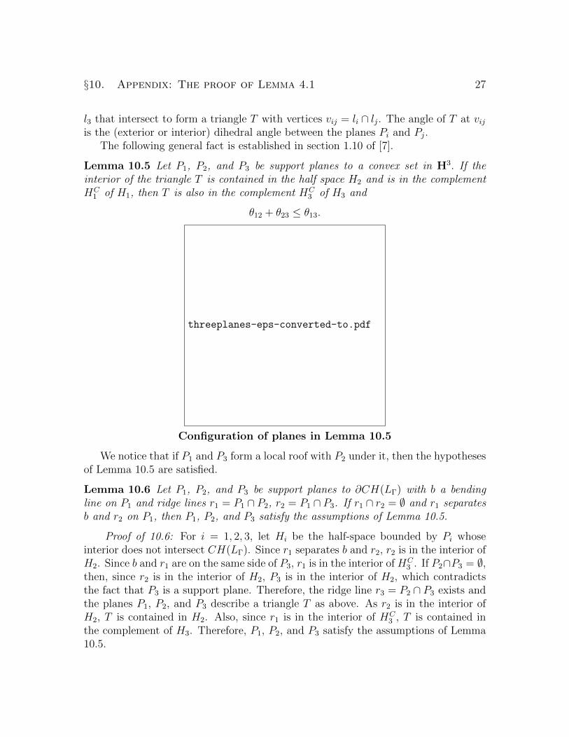
The following general fact is established in section 1.10 of [7].

Lemma 10.5 Let P1, P2, and P3 be support planes to a convex set in H3. If theinterior of the triangle T is contained in the half space H2 and is in the complementHC

1 of H1, then T is also in the complement HC3 of H3 and

θ12 + θ23 ≤ θ13.

threeplanes-eps-converted-to.pdf

Configuration of planes in Lemma 10.5

We notice that if P1 and P3 form a local roof with P2 under it, then the hypothesesof Lemma 10.5 are satisfied.

Lemma 10.6 Let P1, P2, and P3 be support planes to ∂CH(LΓ) with b a bendingline on P1 and ridge lines r1 = P1 ∩ P2, r2 = P1 ∩ P3. If r1 ∩ r2 = ∅ and r1 separatesb and r2 on P1, then P1, P2, and P3 satisfy the assumptions of Lemma 10.5.

Proof of 10.6: For i = 1, 2, 3, let Hi be the half-space bounded by Pi whoseinterior does not intersect CH(LΓ). Since r1 separates b and r2, r2 is in the interior ofH2. Since b and r1 are on the same side of P3, r1 is in the interior of HC

3 . If P2∩P3 = ∅,then, since r2 is in the interior of H2, P3 is in the interior of H2, which contradictsthe fact that P3 is a support plane. Therefore, the ridge line r3 = P2 ∩ P3 exists andthe planes P1, P2, and P3 describe a triangle T as above. As r2 is in the interior ofH2, T is contained in H2. Also, since r1 is in the interior of HC

3 , T is contained inthe complement of H3. Therefore, P1, P2, and P3 satisfy the assumptions of Lemma10.5.


10.6

We are now ready to analyze the situation when the ridge lines are monotonic.

Lemma 10.7 Let α : [0, 1] → ∂CH(LΓ) be a geodesic path which is transverse toβΓ and let Pt| t ∈ [0, k] be a continuous one-parameter family of support planesto α. Suppose that the ridge lines rt = P0 ∩ Pt exist for all t ∈ (0, k] and form amonotonic family of geodesics. Let limt→0rt = b where b is a bending line on P0. Lett1, t2 ∈ (0, k] with t1 < t2.

1. If rt1 is a bending line, then rt = b for t ∈ (0, t1].

2. If rt1 = rt2, then either

Pt = Pt1 for all t ∈ [t1, t2] or rt = b for all t ∈ (0, t2].

3. If Pt1 = Pt2, then Pt = Pt1 for all t ∈ [t1, t2].

4. The exterior dihedral angle θt between P0 and Pt is monotonically increasing.

Proof of 10.7: If rt1 is a bending line b0 and b0 = b, then, by monotonicity, rt = bfor all t ∈ (0, t1]. If b0 6= b then there must be a t3 ∈ (0, t1) such that rt3 separates band b0. Thus either b or b0 is in the interior of Ht3 , the half space corresponding toPt3 . This contradicts the fact that both b and b0 are bending lines. Thus b0 = b andwe have established claim (1).

Suppose that rt1 = rt2 . Then, by monotonicity, rt = rt1 for all t ∈ [t1, t2]. EitherPt = Pt1 for all t ∈ [t1, t2] or there is some t3 ∈ (t1, t2] such that the support planePt3 is not equal to Pt1 or Pt2 . In this case, rt1 is contained in the three distinctsupport planes P0, Pt1 , and Pt3 . Therefore, by Lemma 10.3, rt1 is a bending line b0

on P0. Thus, by claim (1), b0 = b and by monotonicity, rt = b for all t ∈ (0, t2]. Thisestablishes claim (2).

If Pt1 = Pt2 , then rt1 = rt2 . Therefore, by claim (2), either Pt = Pt1 for allt ∈ [t1, t2] or rt = b for all t ∈ (0, t2]. If rt = b for all t ∈ (0, t2], then let X and Ybe the extreme planes at b and let s2 = s(t2). Since α([0, s2]) ⊂ X ∪ Y , it intersectsb only once. So, Pt|t ∈ [t1, t2] sweeps out an arc in Σ(b) joining Pt1 to Pt2 . SincePt1 = Pt2 , Pt must equal Pt1 for all t ∈ [t1, t2]. Thus, in either case, Pt = Pt1 for allt ∈ [t1, t2], which is claim (3).

We now show monotonicity of θt. Let t1 ∈ (0, k], and let s1 = s(t1). It suffices toshow that there exists δ > 0 such that θt ≥ θt1 for all t ∈ [t1, t1 + δ).

If α(s1) is in a flat then there is some δ > 0 so that Pt = Pt1 for all t ∈ [t1, t1 + δ)and therefore θt = θt1 for all t ∈ [t1, t1 + δ) which completes the proof in this case.


Now suppose that α(s1) is contained in a bending line b1 and t2 > t1. If Pt1 = Pt2then θt2 = θt1 . If Pt1 6= Pt2 and rt1 = rt2 then, by claim (2), rt = b for all t ∈ (0, t2].Thus the support planes Pt| t ∈ [0, t2] sweep out an arc in Σ(b) which begins at P0,and again θt1 ≤ θt2 . Therefore, θt1 ≤ θt2 if Pt1 = Pt2 or rt1 = rt2 .

If Pt1 6= Pt2 and rt1 6= rt2 , then, by monotonicity, either rt1 separates b and rt2 , orrt1 = b. If rt1 separates b and rt2 , then we apply Lemma 10.6 to the support planesP0, Pt1 , and Pt2 to see that θt1 ≤ θt2 . By combining the above, we see that if rt1 6= b,then θt1 ≤ θt2 for all t2 ∈ [t1, k].

If rt1 = b, then, by monotonicity, rt = b for all t ∈ [0, t1]. As Pt1 6= P0, b haspositive bending angle. If b is the bending line b1 which contains α(s1), then we maychoose δ > 0 such that if t ∈ [t1, t1 + δ), then Pt is a support plane to b. This impliesthat if t2 ∈ [t1, t1 + δ), then rt1 = rt2 = b. We saw above that this implies thatθt1 ≤ θt2 .

If b 6= b1, we choose a neighborhood N of b1 in the space of geodesics so that nogeodesic in N intersects P0. Lemma 10.1 assures us that we can choose δ > 0 suchthat if t2 ∈ [t1, t1 + δ) and Pt2 6= Pt1 , then rt1,t2 = Pt1 ∩ Pt2 ⊂ N . If Pt1 = Pt2 orrt1 = rt2 , then we have previously shown that θt2 ≥ θt1 . If Pt1 6= Pt2 and rt1 6= rt2 ,then rt1,t2 ⊆ N , so rt1,t2 is in the interior of HC

0 . Furthermore, b does not lie in Pt2 ,so b is in the interior of Hc

t2. In order to apply Lemma 10.5 to the half-spaces H0,

Ht1 and Ht2 , we need to show that rt2 is in the interior of Ht1 . To do this we applya simple continuity argument. Since rt2 6= rt1 = b, there is a t3 ∈ [t1, t2] such that rt3separates b and rt2 . Thus rt2 is in the interior of Ht3 . Moreover, if t ∈ [t1, t3], thenrt ∩ rt2 = ∅. So, for all t ∈ [t1, t3], Pt ∩ rt2 = ∅. We consider the half spaces Ht forall t ∈ [t1, t3]. As rt2 is in the interior of Ht3 and Pt ∩ rt2 = ∅ for all t ∈ [t1, t3], then,by continuity, rt2 is in the interior of Ht for all t ∈ [t1, t3]. In particular, rt2 is in theinterior of Ht1 . Lemma 10.5 then gives that θt1 ≤ θt2 . So, if rt1 = b, we have seenthat there exists δ > 0 such that θt1 ≤ θt2 for all t2 ∈ [t1, t1 + δ). This completes theproof that θt is monotonic.

10.7

We are now ready to establish Lemma 4.1, which we restate here for reference.

Lemma 4.1: Let N = H3/Γ be an analytically finite hyperbolic 3-manifold such thatLΓ is not contained in a round circle. Let α : [0, 1]→ ∂CH(LΓ) be a geodesic arc, inthe intrinsic metric on ∂CH(LΓ), which is transverse to βΓ. If (P,Q) is a roof overα, and Pt| t ∈ [0, k] is the continuous one-parameter family of support planes overα joining P to Q, then

1.i(α, βΓ)QP ≤ θ < π.


where θ is the exterior dihedral angle between P and Q, and

2. there is a t ∈ [0, k] such that Pt = P if t ∈ [0, t] and the ridge linesrt = P ∩ Pt|t > t exist and form a monotonic family of geodesics on P .

Proof of 4.1: We first prove claim (2), that the ridge lines are monotonic. LetPt| ∈ [0, k] be the continuous one-parameter family of support planes along α fromP to Q. We let Ht be the half-space bounded by Pt and let Dt be the closed disk inC associated to Pt.

Since (P,Q) is a roof over α, P0 ∩ Pt 6= ∅ for all t ∈ [0, k]. Let t be the maximumvalue such that Pt = P0 for all t ∈ [0, t]. If t = k, then claim (2) is trivially true.

Consider the case when t < k. Let s = s(t), then α([0, s]) ⊆ P0. If α(s) is in aflat, we obtain a contradiction to the maximality of t. So, α(s) is on a bending line b.Let U be adapted for α(s) and choose k1 > t so that α([t, k1]) ⊂ U . By lemma 10.4,the ridge lines rt for t ∈ (t, k1] are well-defined and monotonic. Also by continuitylim

t→t+ rt = b. Thus, if we define rt = b, we obtain a monotonic family of geodesicsrt for t ∈ [t, k1].

Since (P,Q) is a roof over α, if P0 ∩ Pt is not a ridge line then Pt = P0. Let T bethe maximum value such that the ridge lines rt exist and give a monotonic family ofgeodesics for t ∈ (t, T ). Since PT ∩ P0 6= ∅, either PT = P0 or rT = PT ∩ P0 is a ridgeline.

By lemma 10.7, the angle θt is an increasing function on (t, T ). Since θt ∈ (0, π)for all t ∈ (t, T ), we see that if PT = P0 then θT = π and HT has disjoint interiorfrom H0. This contradicts our assumption that (P,Q) is a roof for α.

Thus we can assume that the ridge line rT exists. Then, by continuity, the familyof geodesics rt| t ∈ (t, T ] is monotonic. If T = k, claim (2) holds. So assume thatT < k.

Let T be the minimum value in [t, T ] such that PT = PT . Thus, since rt ismonotonic on (t, T ), Lemma 10.7 implies that Pt = PT for all t ∈ [T , T ].

We now consider the ridge lines rTt = Pt ∩ PT . By the choice of T there is someδ1 > 0 such that rTt is a ridge line for t ∈ (T − δ1, T ). We define b−T = lim

t→T−rTt .

Similarly, by our choice of T , there is some δ2 > 0 such that rTt is a ridge line fort ∈ (T, T + δ2). We define b+

T = limt→T+rTt . Then b+T and b−T are both bending lines

(possibly equal) on the support plane PT . By definition of T , α(s(T )) ∈ b+T .

As bending lines do not intersect, either b+T = b−T or they are disjoint geodesics on

PT . By Lemma 10.2, if a bending line intersects a ridge line they must be equal, soneither b+

T nor b−T transversely intersect rT .We will establish a contradiction by finding a δ > 0 such that rt is monotonic on

[t, T +δ). We first show that there is a δ > 0 so that rt is monotonic on (T −δ, T +δ).If b+

T intersects P0 then, since ridge lines are equal or disjoint, by Lemma 10.2,rT = b+

T . Therefore, by Lemma 10.7, rt = b for all t ∈ [t, T ]. As PT 6= P0, b has a


positive bending angle. Therefore, there exists δ > 0 such that Pt is a support planeto b+

T = b for all t ∈ (T − δ, T + δ). Therefore, rt = b for all t ∈ (T − δ, T + δ) and isthus trivially monotonic on this region.

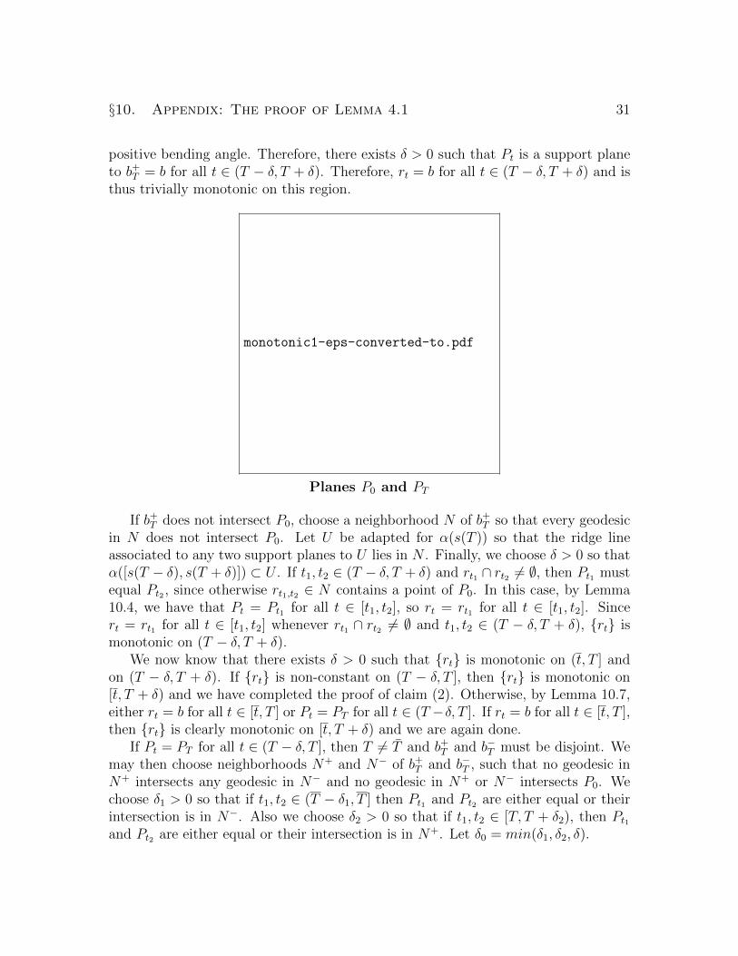
monotonic1-eps-converted-to.pdf

Planes P0 and PT

If b+T does not intersect P0, choose a neighborhood N of b+

T so that every geodesicin N does not intersect P0. Let U be adapted for α(s(T )) so that the ridge lineassociated to any two support planes to U lies in N . Finally, we choose δ > 0 so thatα([s(T − δ), s(T + δ)]) ⊂ U . If t1, t2 ∈ (T − δ, T + δ) and rt1 ∩ rt2 6= ∅, then Pt1 mustequal Pt2 , since otherwise rt1,t2 ∈ N contains a point of P0. In this case, by Lemma10.4, we have that Pt = Pt1 for all t ∈ [t1, t2], so rt = rt1 for all t ∈ [t1, t2]. Sincert = rt1 for all t ∈ [t1, t2] whenever rt1 ∩ rt2 6= ∅ and t1, t2 ∈ (T − δ, T + δ), rt ismonotonic on (T − δ, T + δ).

We now know that there exists δ > 0 such that rt is monotonic on (t, T ] andon (T − δ, T + δ). If rt is non-constant on (T − δ, T ], then rt is monotonic on[t, T + δ) and we have completed the proof of claim (2). Otherwise, by Lemma 10.7,either rt = b for all t ∈ [t, T ] or Pt = PT for all t ∈ (T −δ, T ]. If rt = b for all t ∈ [t, T ],then rt is clearly monotonic on [t, T + δ) and we are again done.

If Pt = PT for all t ∈ (T − δ, T ], then T 6= T and b+T and b−T must be disjoint. We

may then choose neighborhoods N+ and N− of b+T and b−T , such that no geodesic in

N+ intersects any geodesic in N− and no geodesic in N+ or N− intersects P0. Wechoose δ1 > 0 so that if t1, t2 ∈ (T − δ1, T ] then Pt1 and Pt2 are either equal or theirintersection is in N−. Also we choose δ2 > 0 so that if t1, t2 ∈ [T, T + δ2), then Pt1and Pt2 are either equal or their intersection is in N+. Let δ0 = min(δ1, δ2, δ).


We first show that b−T separates rT from b+T . By the definition of T , rt 6= rT for

any t ∈ (T − δ0, T ). Thus, rt separates b and rT in P0. So rT is in the interior of Ht

for any t ∈ (T − δ0, T ). Since b+T and b−T are bending lines they are on the same side

of rTt in PT . Thus b+T is in the interior of HC

t . Therefore rTt separates rT and b+T in

PT . Since rTt tends to b−T as t→ T−

, b−T separates rT and b+T .

If rt1 = rT for some t1 ∈ (T, T + δ0), then, by the monotonicity of rt on(T − δ0, T + δ0), rt = rT for all t ∈ [T, t1) which would imply that rt is monotonicon [t, t1), which would contradict the maximality of T . Suppose that t ∈ (T, T + δ0).Since b−T separates rT and b+

T in PT and rTt lies in N+, b−T separates rT and rTt inPT . Thus, rT is in the interior of HC

t . If rt separates b from rT on P0, then b is inthe interior of Ht. This contradicts the fact that b is a bending line. Thus, for allt ∈ (T, T+δ0), rT separates b and rt on P0. Therefore, rt is monotonic on (t, T+δ0).This completes the proof of claim (2).

We now prove claim (1) by induction on the number of local roofs. If (P,Q) isa local roof over α then i(α, βΓ)QP ≤ θ < π by the definition of intersection number.Assume now that we have established claim (1) for any arc which is covered by n− 1local roofs and that α is covered by n local roofs with the ith having boundary supportplanes Pti−1

and Pti , so that Pt0 = P0 and Ptn = Pk. Let θi,j be the exterior dihedralangle between Pti and Ptj and let rti = P0 ∩ Pti . It follows from the definition of thebending measure and our inductive assumption, that

i(α, βΓ)QP ≤ θ0,n−1 + θn−1,n.

If Ptn = Ptn−1 , then θn−1,n = 0 and so

i(α, βΓ)QP = i(α, βΓ)Pn−1

P ≤ θ0,n−1 = θ

If Ptn 6= Ptn−1 , then we consider the ridge lines rtn−1 and rtn . If rtn−1 = rtn then, asPtn 6= Ptn−1 , Lemma 10.7 implies that rt = b for all t ∈ (t, k]. Thus, Pt| t ∈ [0, k]sweeps out an arc in Σ(b) with total angle θ and

i(α, βΓ)QP = θ.

If rtn−1 6= rtn then either rtn−1 separates b and rtn or rtn−1 = b. If rtn−1 separatesb and rtn then, by Lemma 10.6, the half-spaces H0, Htn−1 , and Htn satisfy Lemma10.5, so θ0,n−1 + θn−1,n ≤ θ0,n and therefore

i(α, βΓ)QP ≤ θ0,n = θ

Now consider the case with rtn−1 6= rtn and rtn−1 = b. Let r = Ptn−1 ∩ Ptn . Toapply lemma 10.5, we need to show that b is in the interior of HC

tn and that rtn is in

REFERENCES 33

the interior of Htn−1 . Since b is a bending line which does not meet Htn , b lies in theinterior of HC

tn . Since rtn−1 6= rtn , Lemma 10.7 implies that rtn is not a bending line.Choose ta ∈ [tn−1, tn], such that rta separates b and rtn . Thus, rtn is in the interiorof Hta and for all t ∈ [tn−1, ta], rt = Pt ∩ P0 is between b and rta , so Pt ∩ rtn = ∅.Considering the half-spaces Ht for t ∈ [tn−1, ta], we note that rtn is in the interior ofHta and Pt∩rtn = ∅ for all t ∈ [tn−1, ta]. Therefore, by continuity, rtn is in the interiorof Ht for all t ∈ [tn−1, ta]. In particular, rtn is in the interior of Htn−1 . Applyinglemma 10.5 we have that θ0,n−1 + θn−1,n ≤ θ0,n and therefore, again,

i(α, βΓ)QP ≤ θ0,n = θ.

4.1

References

[1] L.V. Ahlfors, “Finitely generated Kleinian groups,” Amer. J. of Math. 86(1964), 413–429.

[2] F. Bonahon, “Bouts des varietes hyperboliques de dimension 3,” Ann. of Math. 124(1986),71–158.

[3] F. Bonahon, “The geometry of Teichmuller space via geodesic currents,” Invent. Math.92(1988), 139–162.

[4] M. Bridgeman, “Average bending of convex pleated planes in hyperbolic three-space,” Invent.Math. 132(1998), 381–391.

[5] P. Buser, Geometry and Spectra of Compact Riemann Surfaces, Birkhauser, 1992.

[6] R.D. Canary, “The conformal boundary and the boundary of the convex core,” Duke Math.J., 106(2001), 193–207.

[7] D.B.A. Epstein and A. Marden, “Convex hulls in hyperbolic space, a theorem of Sullivan,and measured pleated surfaces,” in Analytical and Geometrical Aspects of Hyperbolic Space,Cambridge University Press, 1987, 113–253.

[8] D.B.A. Epstein, A. Marden and V. Markovic, “Quasiconformal homeomorphisms and the con-vex hull boundary,” preprint.

[9] D.B.A. Epstein, A. Marden and V. Markovic, “Complex angle scaling,” preprint.

[10] D.B.A. Epstein and V. Markovic, “The logarithmic spiral: a counterexample to the K = 2conjecture,” preprint.

[11] C.T. McMullen, “Complex earthquakes and Teichmuller theory,” J. Amer. Math. Soc.11(1998), 283–320.

REFERENCES 34

[12] K. Sigmund, “On dynamical systems with the specification property,” Trans. A.M.S.190(1974), 285–299.

[13] W.P. Thurston, The Geometry and Topology of 3-Manifolds, Lecture Notes, Princeton Univer-sity, 1979.

[14] W.P. Thurston, “Minimal stretch maps between hyperbolic surfaces,” preprint, available at:

http://front.math.ucdavis.edu/math.GT/9801058

Documents

canary/martin.pdfFrom the boundary of the convex core to the conformal boundary Martin Bridgeman and Richard D. Canary Department of Mathematics, Boston College, Chestnut Hill, MA