CANDY Manual

Description of Background

Contributors: Uwe Franko, Burkhard Oelschlagel, Stefan Schenk, Martina Puhlmann, Katrin Kuka, Janine Mallast nee Kruger, Enrico Thiel, Nadia Prays, Katharina Meurer, Eric Bonecke CANDY Version 2015

II

III

Table of Contents

MODEL DESCRIPTION ............................................................................................................ 5

INTRODUCTION ............................................................................................................................ 5 Access to soil properties ............................................................................................................................ 6 Access to climate data ............................................................................................................................... 6 Access to management data ..................................................................................................................... 6 Access to measurement data .................................................................................................................... 6 Access to parameter tables ....................................................................................................................... 6 Generation of result records ..................................................................................................................... 6 Process modules ........................................................................................................................................ 7 Good modelling practice ........................................................................................................................... 7

DESCRIPTION OF PROCESS MODULES ................................................................................... 8

SOIL TEMPERATURE DYNAMICS ........................................................................................................ 8 Input .......................................................................................................................................................... 8 Output ....................................................................................................................................................... 8 Parameters ................................................................................................................................................ 8 Description................................................................................................................................................. 8

SOIL WATER DYNAMICS ................................................................................................................ 11 Input ........................................................................................................................................................ 11 Output ..................................................................................................................................................... 11 Parameters .............................................................................................................................................. 11 Description............................................................................................................................................... 11

Percolation ................................................................................................................................................... 14 Interception ................................................................................................................................................. 15 Snow accumulation and melting ................................................................................................................. 15 Evapotranspiration ...................................................................................................................................... 15

SOIL STRUCTURE DYNAMICS .......................................................................................................... 17 Input ........................................................................................................................................................ 17 Output ..................................................................................................................................................... 17 Parameters .............................................................................................................................................. 17 Description............................................................................................................................................... 17

Bulk density.................................................................................................................................................. 18 Soil loosening ........................................................................................................................................... 18 Re-compaction ......................................................................................................................................... 18 Cryoturbation .......................................................................................................................................... 19 Bioturbation ............................................................................................................................................. 19

PEDOTRANSFERFUNCTIONS IN CANDY ............................................................................................ 20 Soil texture class conversion ........................................................................................................................ 20 Bulk density.................................................................................................................................................. 20 Particle density ............................................................................................................................................ 20 Pore Volume ................................................................................................................................................ 21 Water parameters according to Lieberoth .................................................................................................. 21 Water retention model according to van Genuchten .................................................................................. 21

Approach of Vereecken ........................................................................................................................... 21 Approach of Zacharias & Wessolek ......................................................................................................... 22

Water retention model according to Brooks-Corey ..................................................................................... 23 Approach of Rawls and Brakensiek ......................................................................................................... 23

BIOLOGIC ACTIVE TIME ................................................................................................................ 25 Input ........................................................................................................................................................ 25 Output ..................................................................................................................................................... 25 Description............................................................................................................................................... 25

IV

SOIL ORGANIC MATTER TURNOVER .................................................................................................. 27 Approach with conceptual pools ................................................................................................................. 27

Input ........................................................................................................................................................ 27 Output ..................................................................................................................................................... 27 Parameters .............................................................................................................................................. 27 Description............................................................................................................................................... 27

Carbon In Pore Space (CIPS) approach ........................................................................................................ 30 Input ........................................................................................................................................................ 30 Output ..................................................................................................................................................... 30 Parameters .............................................................................................................................................. 30 Description............................................................................................................................................... 31

N DYNAMICS ............................................................................................................................. 36 Input ........................................................................................................................................................ 36 Output ..................................................................................................................................................... 36 Parameters .............................................................................................................................................. 36 Description............................................................................................................................................... 37

Nitrogen Sources ......................................................................................................................................... 38 N deposition ............................................................................................................................................ 38 Input from land management ................................................................................................................. 38 Organic amendments .............................................................................................................................. 39 Mineralisation / Immobilisation .............................................................................................................. 39 N fixation by legume crop........................................................................................................................ 39

Nitrogen sinks .............................................................................................................................................. 39 Plant uptake ............................................................................................................................................. 39 N losses .................................................................................................................................................... 39

CROP MODULE ........................................................................................................................... 42 Crop development ....................................................................................................................................... 42 CANDY_S approach ...................................................................................................................................... 42

Input ........................................................................................................................................................ 42 Output ..................................................................................................................................................... 42 Parameters .............................................................................................................................................. 42 Description............................................................................................................................................... 44

Legumes ....................................................................................................................................................... 46 Input ........................................................................................................................................................ 46 Output ..................................................................................................................................................... 46 Parameter ................................................................................................................................................ 46 Description............................................................................................................................................... 46

Permanent Grasslands ................................................................................................................................. 47 Input ........................................................................................................................................................ 47 Output ..................................................................................................................................................... 47 Parameters .............................................................................................................................................. 47 Description............................................................................................................................................... 47

LITERATURE .......................................................................................................................... V

5

Model description

Introduction The agro-ecosystem model CANDY (Carbon And Nitrogen DYnamics) has been developed to describe carbon and nitrogen dynamics in arable soils in order to provide information about carbon stocks in soils, organic matter turnover, nitrogen uptake by crops, leaching and water quality.

It consists of a modular system of sub models and a data base system for model parameters, initial soil values, weather data, soil management data and measurement values. The user interface of the model provides geographic information system facilities that are designed to organize regional scenario simulations.

Model specific input data comprises soil and plant properties as well as process parameters, user or scenario related data to describe the agricultural management, climate and observed features.

The model results consist of soil and crop related state variables and fluxes connected to soil organic matter, nitrogen and water.

Special features are:

• CANDY calculates a biologic active time (BAT) which allows the assessment of organic matter turnover for different sites and gives the possibility to calculate the steady state of soil organic matter.

• A weather generator provides the possibility to simulate long term scenarios repeating a given crop rotation several times.

• An optional auto fertilizer scheme (SBA) implements good farming practices for mineral nitrogen application.

• The optional CIPS approach describes the relevance of soil structure for the long term stabilization of soil organic matter.

The CANDY model started its history as an integrated simulation tool for carbon and nitrogen dynamics in soils providing a user interface to handle input and output data. During a number of projects and with the input of many people more and more adjustments have been made in order to make the model usable for the specific task. Now we speak about CANDY as a system consisting of a number of modules where some of them are mandatory for ecosystem modelling because they provide the infrastructure and other may be switched on or off depending on the objective and the available data. There are for instance different modules for crop dynamics and for SOM turnover as well.

To make things more complex the modules may have different parameters. Because of this reason any user has to develop a clear idea about the objective of the modelling work and the required database. It is necessary to check the available parameter tables if they contain already the required information.

6

The CANDY infrastructure covers the main processes that are relevant for an agro-ecosystem and the required facilities for the data management:

Access to soil properties Soil is in the main focus of CANDY. Each simulation is performed on a specific soil considering a sequence of agricultural activities and a specific weather course. The soil is regarded as one dimensional profile consisting of separate horizons that are mainly characterized by soil texture and a set of soil physical properties. In contrast to natural horizon dimensions the model regards the soil profile as sequence of homogenous layers of 1 dm thickness. Depending on the chosen simulation mode, the physical properties can be handled as parameters (constant values over time) or as state variables with an inherent dynamics.

Access to climate data Climate data are usually available as daily observations but CANDY can also use a climate generator or aggregated climate values. In any case the climate module delivers daily values to all other sub-models.

Access to management data This module distributes the management information to the appropriate sub-models. Sometimes this requires some search activities in the data and the breakdown for instance of a slurry amendment into mineral fertilization, adding of organic matter and water input. Each tillage operation leads to averaging of the state variables of the affected calculation layers.

Access to measurement data All measurement data are stored within a specific table. During the preparation of a simulation run all or selected data are temporarily moved to another table that is used by the model. This table may also include data records that are not based on real observations and are only used to get information from the model. After simulations that take very long time, it may be useful to move the result data from the temporary table back into the permanently stored part.

Access to parameter tables All parameters are accessible over an user interface. In some cases (e.g. soil data) there is a specific interface. In other cases the data administration requires more knowledge about the data organisation. An additional SQL-module supports user that have no separate software for database management available.

Generation of result records Beside the interface to the measurements users may select a number of predefined results in an appropriate time resolution. This is less flexible but the preparation is usually easier.

7

Process modules The basic process modules are: soil water dynamics, soil temperature dynamics, crop development including permanent grassland and livestock, soil organic matter turnover and nitrogen dynamics.

Good modelling practice It is strongly recommended to start with a critical evaluation of the model and the parameters because some specifics of the site or the management system may lead to different results than expected. In this case a new calibration may be required or some more work is necessary to identify additional processes that are not yet included in the model.

CANDY is a system in continuous development. This means that the reliability of the single modules may be different. Some are used with good results over many years and other are rather new with only limited results.

8

Description of process modules The following chapters present the currently available modules. Each chapter is starting with an overview about the inputs, outputs and parameters, including the source of the parameter, its measurement id that can be find in the table CND_MWML as well as the result id from table CDY_RSLT. This part is then followed by description of the algorithms used.

Soil temperature dynamics Input symbol description unit source Tair daily mean air temperature [°C] CDY_CLDAT Ө soil moisture [Vol. %] Internal

Output symbol description unit measurement id result id Ts soil temperature [°C] 9 110 (0-3 dm)

Parameters symbol description unit source HKAP specific heat capacity of the dry soil [J cm-3 K-1] CNDHRZN α thermal conductivity (const.) [J s-1 cm-1 K-1] Internal AMP amplitude [°C] CDYBTPRM PHA phase shift of the sinus/cosinus

function [d] CDYBTPRM

LTEM mean annual air temperature [°C] CDY_FXDAT

Description Soil temperature plays an important role in many processes in the soil, such as chemical reactions and biological interactions. Soil temperature varies in response to exchange processes that primarily take place via the soil surface.

The soil temperature influences the soil water viscosity and thereby the water fluxes within the profile. The influence on the C/N turnover in the model is considered by a reduction function during calculating the Biological Active Time (see chapter 3.3).

The state variable of the temperature module is the soil temperature (Ts). It is modelled by solving the heat flow equation after Suckow (1987) (Equation 1).

∂(HKAP∙Ts)∂t

= ∂∂z�α ∂Ts

∂z� (1)

t time [d] z depth [cm] HKAP specific heat capacity of moist soil [J cm-3 K-1]

9

Ts soil temperature [K] α thermal conductivity of moist soil [J s-1 cm-1 K-1]

Two boundary conditions for Equation 1 have to be given. The upper boundary of soil temperature (at 5 cm depth) is defined as the weighted mean of the air temperatures of the present day, yesterday and the day before yesterday, multiplied by a time-dependent correction factor. The correction is done in order to take into account the neglected meteorological elements and for the crop influence on surface temperature.

As the lower boundary condition (zero heat flow) is assumed at a depth of 200 cm. The soil temperature distribution within the profile is calculated using the air temperature and the lower boundary condition. The soil temperature at 200 cm is calculated depending on the season of the year, either summer (120 < Julian day < 304, Equation 2) or winter (Equation 3).

Lower boundary (summer):

dS = AMP ∙ sin �(dnr + PHA) ∙ 2π365� + LTEM (2)

ds daily soil temperature in summer time [°C] AMP amplitude [°C] sin sinus function dnr Julian day PHA phase shift of the sinus function [d] π Pi LTEM mean annual air temperature [°C]

Lower boundary (winter):

dW = AMP ∙ cos �(dnr + PHA) ∙ 2π365� + LTEM (3)

dw daily soil temperature in winter time [°C] AMP Amplitude [°C] cos cosinus function dnr Julian day PHA phase shift of the cosinus function [d] π Pi LTEM mean annual air temperature [°C]

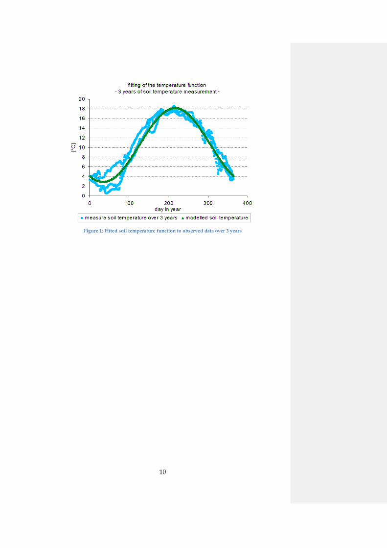
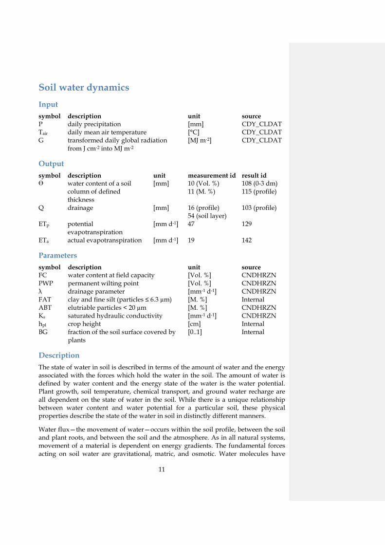
In order to fit simulated to measured data, the parameters AMP and PHA (table CDYBTPRM) can be calibrated. The mean air temperature (LTEM from table CDY_FXDAT) has an influence as well, according to the summer or winter period. The parameters AMP, PHA and LTEM should be fitted to the temperature curve of several years (Figure 1).

10

Figure 1: Fitted soil temperature function to observed data over 3 years

11

Soil water dynamics Input symbol description unit source P daily precipitation [mm] CDY_CLDAT Tair daily mean air temperature [°C] CDY_CLDAT G transformed daily global radiation

from J cm-2 into MJ m-2 [MJ m-2] CDY_CLDAT

Output symbol description unit measurement id result id ϴ water content of a soil

column of defined thickness

[mm] 10 (Vol. %) 11 (M. %)

108 (0-3 dm) 115 (profile)

Q drainage [mm] 16 (profile) 54 (soil layer)

103 (profile)

ETp potential evapotranspiration

[mm d-1] 47 129

ETa actual evapotranspiration [mm d-1] 19 142

Parameters symbol description unit source FC water content at field capacity [Vol. %] CNDHRZN PWP permanent wilting point [Vol. %] CNDHRZN λ drainage parameter [mm-1 d-1] CNDHRZN FAT clay and fine silt (particles ≤ 6.3 µm) [M. %] Internal ABT elutriable particles < 20 µm [M. %] CNDHRZN Ks saturated hydraulic conductivity [mm-1 d-1] CNDHRZN hpl crop height [cm] Internal BG fraction of the soil surface covered by

plants [0..1] Internal

Description The state of water in soil is described in terms of the amount of water and the energy associated with the forces which hold the water in the soil. The amount of water is defined by water content and the energy state of the water is the water potential. Plant growth, soil temperature, chemical transport, and ground water recharge are all dependent on the state of water in the soil. While there is a unique relationship between water content and water potential for a particular soil, these physical properties describe the state of the water in soil in distinctly different manners.

Water flux—the movement of water—occurs within the soil profile, between the soil and plant roots, and between the soil and the atmosphere. As in all natural systems, movement of a material is dependent on energy gradients. The fundamental forces acting on soil water are gravitational, matric, and osmotic. Water molecules have

12

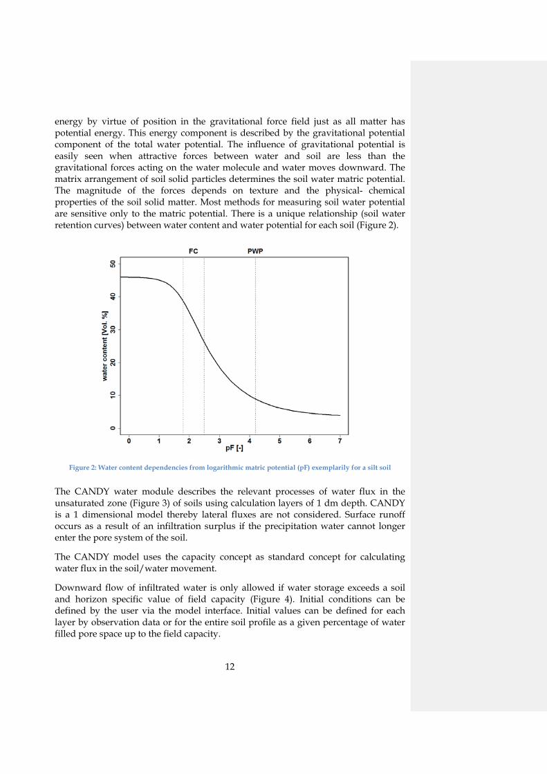
energy by virtue of position in the gravitational force field just as all matter has potential energy. This energy component is described by the gravitational potential component of the total water potential. The influence of gravitational potential is easily seen when attractive forces between water and soil are less than the gravitational forces acting on the water molecule and water moves downward. The matrix arrangement of soil solid particles determines the soil water matric potential. The magnitude of the forces depends on texture and the physical- chemical properties of the soil solid matter. Most methods for measuring soil water potential are sensitive only to the matric potential. There is a unique relationship (soil water retention curves) between water content and water potential for each soil (Figure 2).

Figure 2: Water content dependencies from logarithmic matric potential (pF) exemplarily for a silt soil

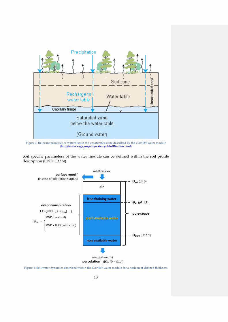
The CANDY water module describes the relevant processes of water flux in the unsaturated zone (Figure 3) of soils using calculation layers of 1 dm depth. CANDY is a 1 dimensional model thereby lateral fluxes are not considered. Surface runoff occurs as a result of an infiltration surplus if the precipitation water cannot longer enter the pore system of the soil.

The CANDY model uses the capacity concept as standard concept for calculating water flux in the soil/water movement.

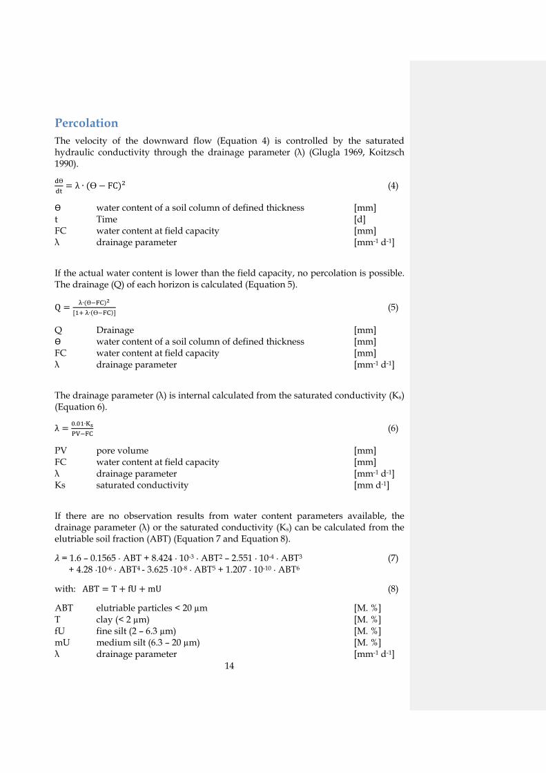
Downward flow of infiltrated water is only allowed if water storage exceeds a soil and horizon specific value of field capacity (Figure 4). Initial conditions can be defined by the user via the model interface. Initial values can be defined for each layer by observation data or for the entire soil profile as a given percentage of water filled pore space up to the field capacity.

13

Figure 3: Relevant processes of water flux in the unsaturated zone described by the CANDY water module

(http://water.usgs.gov/edu/watercycleinfiltration.html)

Soil specific parameters of the water module can be defined within the soil profile description (CNDHRZN).

Figure 4: Soil water dynamics described within the CANDY water module for a horizon of defined thickness

14

Percolation The velocity of the downward flow (Equation 4) is controlled by the saturated hydraulic conductivity through the drainage parameter (λ) (Glugla 1969, Koitzsch 1990).

dӨdt

= λ ∙ (ϴ− FC)2 (4) Ө water content of a soil column of defined thickness [mm] t Time [d] FC water content at field capacity [mm] λ drainage parameter [mm-1 d-1]

If the actual water content is lower than the field capacity, no percolation is possible. The drainage (Q) of each horizon is calculated (Equation 5).

Q = λ∙(Ө−FC)2

[1+ λ∙(ϴ−FC)] (5)

Q Drainage [mm] Ө water content of a soil column of defined thickness [mm] FC water content at field capacity [mm] λ drainage parameter [mm-1 d-1]

The drainage parameter (λ) is internal calculated from the saturated conductivity (Ks) (Equation 6).

λ = 0.01∙KsPV−FC

(6) PV pore volume [mm] FC water content at field capacity [mm] λ drainage parameter [mm-1 d-1] Ks saturated conductivity [mm d-1]

If there are no observation results from water content parameters available, the drainage parameter (λ) or the saturated conductivity (Ks) can be calculated from the elutriable soil fraction (ABT) (Equation 7 and Equation 8).

𝜆𝜆 = 1.6 – 0.1565 ∙ ABT + 8.424 ∙ 10-3 ∙ ABT2 – 2.551 ∙ 10-4 ∙ ABT3 (7) + 4.28 ∙10-6 ∙ ABT4 - 3.625 ∙10-8 ∙ ABT5 + 1.207 ∙ 10-10 ∙ ABT6

with: ABT = T + fU + mU (8)

ABT elutriable particles < 20 µm [M. %] T clay (< 2 µm) [M. %] fU fine silt (2 – 6.3 µm) [M. %] mU medium silt (6.3 – 20 µm) [M. %] λ drainage parameter [mm-1 d-1]

15

If water storage exceeds the pore volume of a calculation layer the amount surplus water is added to the calculation layer above. If the soil surface is reached the soil water is considered as runoff or puddle. The maximum water storage of the puddle (MPH) is calculated in mm (Equation 9).

𝑀𝑀𝑀𝑀𝑀𝑀 = 40.667 + 0.592 ∙ 𝐹𝐹𝐹𝐹𝑢𝑢𝑢𝑢𝑢𝑢𝑢𝑢𝑢𝑢_𝑙𝑙𝑙𝑙𝑙𝑙𝑢𝑢𝑢𝑢 (9)

Interception The interception of water by a crop (Equation 10) depends on the crop height (Koitzsch 1990, Koitzsch and Günther 1990).

Ci = 2.5 ∙ BG ∙ hpl (10)

Ci interception capacity [mm] hpl crop height [cm] BG fraction of the soil surface covered by plants [0..1]

Snow accumulation and melting The process of snow accumulation and melting is calculated according to Koitzsch (1990): snow fall is only possible if rainfall occurs and mean daily temperature is ≤ 0.5 °C. Melting and infiltration can occur during mean daily temperature > 0.5 °C.

Evapotranspiration Evapotranspiration in the CANDY water module is allowed if water storage exceeds a soil and horizon specific value of minimum water content (Figure 4). The process of evaporation is calculated with a modified TURC – equation, based on the work of Koitzsch and Günther (Turc 1961, Koitzsch 1990, Koitzsch and Günther 1990). The calculation of potential evapotranspiration (Equation 11, Equation 12 and Equation 13) and actual evapotranspiration (Equation 14) is according to Koitzsch (1990).

ETp = (1 + 0.004 ∙ h) ∙ Ep ; h ≤ 100 (11)

ETp potential evapotranspiration [mm d-1] h crop height [cm] Ep value of pan evaporation [mm d-1] with:

Ep = 0.0041 ∙ (Tair + 22.7) ∙ (G + 2.09) (12)

Ep value of pan evaporation [mm d-1] Tair air temperature [°C] G daily global radiation [MJ m-2]

16

EIp = 1.3 ∙ Ep (13)

EIp potential evaporation of intercepted water by crop [mm d-1] Ep value of pan evaporation [mm d-1]

ETa = 0.5 min�EIp, Ri� + Ψ ∙ H1 max �0, �1 − RiEIp� ∙ ETp� + (1 −Ψ) ∙ H2 ∙ Ep (14)

ETa actual evapotranspiration [mm d-1] Ri intercepted water [mm d-1] Ψ fraction of the soil surface covered by transpiring plants H1, H2 reduction coefficients calculated as funct. of water content ETp potential evapotranspiration [mm d-1] EIp potential evaporation of intercepted water by crop [mm d-1] Ep value of pan evaporation [mm d-1]

17

Soil structure dynamics Input symbol description unit source P daily precipitation [mm] CDY_CLDAT Tair daily mean air temperature [°C] CDY_CLDAT BAT Biologic Active Time [d] internal

Output symbol description unit measurement id result id TRD bulk density [g cm-3] 63 704 (0-3 dm) TSD particle density [g cm-3] 64 PV pore volume [Vol. %] 65 FC field capacity [Vol. %] 61 PWP permanent wilting point [Vol. %] 62

Parameters symbol description unit source f_bioturb optional parameter to convert BAT

into daily bulk density change [g cm-3 d-1] CDYAPARM

All other parameters are determined internally. Therefor see Equation 15 to Equation 25 in this chapter.

Description Further enhancement of the CANDY model system is related to the integration of the CIPS model (see OM-turnover) and the implementation of a module for the dynamic description of soil structure.

Please be aware that this module is still in development and may require special calibrations to different site conditions.

If this option is activated, the following parameters of soil structure become state variables:

• Bulk density • Particle density • Pore volume (as defined by the both values above) • Field capacity • Permanent wilting point The soil parameters have to be quantified with an additional specification of the Corg content that relates to these values and the site specific value of aggregate density as a maximum value for soil compaction.

Field capacity and permanent wilting point can be calculated using the Brooks-Corey approach for the water retention curve with the pedotransfer function from Rawls

18

and Brakensiek (1985). An alternative approach is the Van Genuchten (1980) model with the pedotransfer function from either Vereecken et al. (1989) or Zacharias and Wessolek (2007) . The detailed description of the implemented functions is given in chapter Pedotransferfunctions.

Bulk density Soil structure depends on bulk density (BD) and the organic carbon concentration of soil. The BD is influenced by management activities and climatic conditions. Soil loosening (disaggregation) (Equation 15) occurs as a result of soil tillage, bio- and cryoturbation (Equation 20 to Equation 22). Further technical compaction is neglected at this model stage. A re-compaction takes place because of natural processes, such as sedimentation of soil, and technically caused by the load of agricultural machineries (Equation 17 to Equation 19).

Soil loosening by tillage and the natural re-compaction are described with model approaches of Schaaf (1998).

Soil loosening

BDnew = BDold − ef ∙ �BDold −23∙ BD0� (15)

BDnew, BDold bulk density [g cm-3] BD0 bulk density after complete re-compaction [g cm-3] ef loosening efficiency of soil tillage tool [0..1]

Re-compaction

BDnew = BDold + (BD0 − BDold) ∙ � RR+exp(3.735−0.08835∙h)� (16)

BDnew, BDold bulk density [g cm-3] BD0 bulk density after complete re-compaction [g cm-3] R factor of re-compaction [-] h lower boundary layer [dm]

The factor of re-compaction (R) results from water percolation, depth and sand content of the corresponding horizon and provides the possibility to calculate the actual bulk density (Equation 17).

R = P ∙ �1+2∙ S

S+exp(8.597−0.075∙S)

(10∙h)0.6 � (17)

R factor of re-compaction [-] P water percolation [mm] S sand content [%] h lower boundary layer [dm]

19

The bulk density after re-compaction (BD0) is calculated by an approach of Ruehlmann and Körschens (2009) depending on actual Corg content at every time step (Equation 18).

BD = (2.631 + 15.811 ∙ b) ∙ exp�b ∙ Corg� (18)

The parameter b is determined site specifically during model initialisation. For a static calculation of bulk density Equation 24 can be used. Usually the observed BD is related to a specific sedimentation status of the soil. As a consequence, it is necessary to implement a re-compaction level (Equation 19).

𝐵𝐵𝐵𝐵0 = 𝐵𝐵𝐵𝐵(𝐹𝐹𝑜𝑜𝑢𝑢𝑜𝑜) ∙ 𝑅𝑅𝐹𝐹 (19)

BD0 bulk density after complete re-compaction [g cm-3] RC re-compaction level [> 0] BD(Corg) observed BD [dm]

For practical reasons, bulk density measurements are usually not performed on a recently loosened soil. Therefore RC will be close to 1.

Cryoturbation If the frozen soil water is thawing within one time step, the volume change is included into the bulk density calculation (Equation 20 and Equation 21).

𝑀𝑀𝑃𝑃 = 𝜀𝜀𝐿𝐿 + 𝜀𝜀𝑊𝑊 ∙ 1.09 (20)

𝐵𝐵𝐵𝐵 = (1 − 𝑀𝑀𝑃𝑃) ∙ 𝑀𝑀𝐵𝐵 (21)

PV pore volume after thawing [0..1] BD bulk density [g cm-3]

Wε relative water volume [0..1]

Lε relative air volume [0..1] PD particle density [g cm-3]

Bioturbation The results of bioturbation are calculated assuming that the change of bulk density is related to the actual BAT value (Equation 22).

∆𝐵𝐵𝐵𝐵 = 𝑓𝑓_𝑏𝑏𝑏𝑏𝑏𝑏𝑏𝑏𝑏𝑏𝑏𝑏𝑏𝑏 ∙ 𝐵𝐵𝐵𝐵𝐵𝐵 (22)

ΔBD change of bulk density (old-new) [g cm-3] f_bioturb parameter [d-1] BAT Biologic Active Time [d]

The parameter f_bioturb can be defined in the general parameters (CDYAPARM) – otherwise the standard value 0.001 is used.

20

Pedotransferfunctions in CANDY Modelling of processes and turnover in agro ecosystems requires detailed information about the soil and soil water balance. Since measurements of soil physical parameters are time consuming and expensive, application of pedotransfer functions is an appropriate alternative. This enables the estimation of required soil properties (e.g. field capacity, permanent wilting point) from other known and easily measureable properties (e.g. texture). Furthermore, the implementation of the dynamical description of soil structure in CANDY bases on the application of pedotransfer functions (e.g. bulk density) (see chapter Soil structure dynamics).

Soil texture class conversion In some approaches the soil texture is based on the USDA7 system. This system defines clay as the particle size fraction < 2 µm, silt as the fraction between 2 and 50 µm and sand as the fraction between 50 and 2000 µm. For converting the German soil system into the USDA7 system, the following interpolation (Equation 26) after Nemes et al. (1999) is useful.

STK = y2−y1log(x2)−log(x1) ∙ (log(x) − log(x1)) + y1 (23)

STK soil texture class [M. %] x particle size diameter of the missing STK (upper limit) [mm] y1 cumulative percentage on the particle-size distribution curve

with the next small particle size diameter [M. %]

y2 cumulative percentage on the particle-size distribution curve with the next bigger particle size diameter

[M. %]

x1, x2 corresponding particle size diameters to y1 and y2 [mm]

Bulk density The dynamic of bulk density is described in chapter Soil structure dynamics (Equation 18). If only clay content and Corg content are available it is possible to calculate bulk density using Equation 24 (Ruehlmann and Körschens 2009).

𝐵𝐵𝑅𝑅𝐵𝐵 = 1.64 − 0.0075 ∙ 𝐵𝐵 − 0.0611 ∙ 𝐹𝐹𝑜𝑜𝑢𝑢𝑜𝑜 (24)

Particle density The particle density PD is calculated following an approach depending on actual Corg (Equation 23 to Equation 25) (Rühlmann et al. 2006).

PD = �QOSρOS

+ 1−QOSρmin

�−1

(25)

With:

21

ρOS = 1.127 + 0.373 ∙ QOS (26)

QOS = Corg55

(27)

QOS volumetric part of organic matter [-] Corg organic carbon content [M. %]

OSρ density of organic matter [g cm-3] PD particle density [g cm-3]

minρ density of mineral substance (site specific parameter - initialisation phase)

[g cm-3]

Pore Volume The pore volume is based on the relation between bulk density and particle density.

𝑀𝑀𝑃𝑃 = 1 − 𝑇𝑇𝑇𝑇𝑇𝑇𝑇𝑇𝑇𝑇𝑇𝑇

(28)

Water parameters according to Lieberoth The simplest approach to calculate field capacity (Equation 27) and permanent wilting point (Equation 28) after Lieberoth (1982) is based on soil texture data only.

FC = 3.4 + 0.85 ∙ ABT (29)

PWP = 1.23 + 0.74 ∙ T (30)

FC water content at field capacity [mm] ABT particles < 20 µm [M. %] PWP permanent wilting point [mm] T clay content (< 2 µm ) [M. %]

Water retention model according to van Genuchten Ө(𝛹𝛹) = Ө𝑢𝑢 + Ө𝑠𝑠−Ө𝑟𝑟

(1+(𝛼𝛼∙|𝛹𝛹|)𝑛𝑛)𝑚𝑚 (31)

α van Genuchten parameter [cm-1] n van Genuchten parameter [-] m van Genuchten parameter [-] Ψ matric potential [hPa] Өr residue water content [0..1] Өs saturation water content [0..1]

Approach of Vereecken Vereecken et al. (1989) calculate the van Genuchten parameters using USDA7 texture classes (Equation 30 to Equation 34).

22

Ө𝑠𝑠 = 0.81 − 0.283 ∙ 𝐵𝐵𝐵𝐵 + 0.001 ∙ 𝐵𝐵 (32)

Ө𝑢𝑢 = 0.015 − 0.005 ∙ 𝐵𝐵 + 0.014 ∙ 𝐹𝐹𝑜𝑜𝑢𝑢𝑜𝑜 (33)

𝛼𝛼 = 𝑒𝑒�−2.486+0.025∙𝑇𝑇−0.351∙𝐶𝐶𝑜𝑜𝑟𝑟𝑜𝑜−2.617∙𝐵𝐵𝑇𝑇−0.023∙𝑇𝑇� (34)

𝑛𝑛 = 𝑒𝑒(0.053−0.009∙𝑇𝑇−0.013∙𝑇𝑇+0.00015∙𝑇𝑇2) (35)

𝑚𝑚 = 1 (36)

α van Genuchten parameter [cm-1] n van Genuchten parameter [-] m van Genuchten parameter [-] Ψ matric potential [hPa] Өr residue water content [0..1] Өs saturation water content [0..1]

Approach of Zacharias & Wessolek Zacharias and Wessolek (2007) calculated the Van Genuchten parameters without using the organic carbon content based on USDA7 texture classes (Equation 35 to Equation 44).

For S < 66.5

Ө𝑠𝑠 = 0.788 − 0.263 ∙ 𝐵𝐵𝐵𝐵 + 0.001 ∙ 𝐵𝐵 (37)

Ө𝑢𝑢 = 0 (38)

𝛼𝛼 = 𝑒𝑒(−0.648+0.023∙𝑇𝑇−3.1618∙𝐵𝐵𝑇𝑇−0.044∙𝑇𝑇) (39)

𝑛𝑛 = 1.392 + 1.212 ∙ 𝐵𝐵 − 0.4189 ∙ 𝑆𝑆−0.024 (40)

𝑚𝑚 = 1 − 1𝑛𝑛 (41)

For S ≥ 66.5

Ө𝑠𝑠 = 0.89 − 0.322 ∙ 𝐵𝐵𝐵𝐵 + 0.001 ∙ 𝐵𝐵 (42)

Ө𝑢𝑢 = 0 (43)

𝛼𝛼 = 𝑒𝑒(−4.197+0.013∙𝑇𝑇−0.276∙𝐵𝐵𝑇𝑇−0.076∙𝑇𝑇) (44)

𝑛𝑛 = −2.562 + 3.75 ∙ 𝐵𝐵−0.016 + 7 ∙ 10−9 ∙ 𝑆𝑆4.004 (45)

𝑚𝑚 = 1 − 1𝑛𝑛 (46)

α van Genuchten parameter [cm-1] n van Genuchten parameter [-] m van Genuchten parameter [-] Өr residue water content [0..1] Өs saturation water content [0..1]

23

T clay content [M. %] S sand content [M. %] BD bulk density [g cm-3]

Water retention model according to Brooks-Corey

Ө(Ψ) = �Өr + (Өs − Өr) ∙ �ΨΨb�−2

ӨS ; Ψ>Ψb>λ>0

Ψ≤Ψb (47)

Ө(Ψ) water content as function of matric potential [Vol. %] Ψ matric potential [hPa] Ψb air entry potential [hPa] Өr residue water content [Vol. %] Өs saturation water content [Vol. %] λ pore size index [-]

Approach of Rawls and Brakensiek Rawls and Brakensiek calculated the Brooks-Corey parameters from pore volume based on USDA7 texture classes (clay and sand fraction) (Equation 46 to Equation 49) (Brooks 1964, Rawls and Brakensiek 1985).

𝛹𝛹𝑏𝑏 = 𝑒𝑒𝑒𝑒𝑒𝑒(5.3396738 + 0.1845038 ∙ 𝐵𝐵 − 2.48394546 ∙ 𝑀𝑀𝑃𝑃 − 0.00213853 ∙ 𝐵𝐵2 − 0.04356349 ∙ 𝑆𝑆 ∙ 𝑀𝑀𝑃𝑃 − 0.61745089 ∙ 𝐵𝐵 ∙ 𝑀𝑀𝑃𝑃 + 0.00143598 ∙ 𝑆𝑆2 ∙ 𝑀𝑀𝑃𝑃2 − 0.00855375 ∙ 𝐵𝐵2 ∙ 𝑀𝑀𝑃𝑃2 − 0.00001282 ∙ 𝑆𝑆2 ∙ 𝐵𝐵 + 0.00895359 ∙ 𝐵𝐵2 ∙ 𝑀𝑀𝑃𝑃 − 0.00072472 ∙ 𝑆𝑆2 ∙ 𝑀𝑀𝑃𝑃 + 0.0000054 ∙ 𝐵𝐵2 ∙ 𝑆𝑆 + 0.5002806 ∙ 𝑀𝑀𝑃𝑃2 ∙ 𝐵𝐵) (48)

𝜆𝜆 = 𝑒𝑒𝑒𝑒𝑒𝑒(−07842831 + 0.0177544 ∙ 𝑆𝑆 − 1.062498 ∙ 𝑀𝑀𝑃𝑃 − 0.00005304 ∙ 𝑆𝑆2 −0.00273493 ∙ 𝐵𝐵2 + 1.11134946 ∙ 𝑀𝑀𝑃𝑃2 − 0.03088295 ∙ 𝑆𝑆 ∙ 𝑀𝑀𝑃𝑃 + 0.00026587 ∙𝑆𝑆2 ∙ 𝑀𝑀𝑃𝑃2 − 0.00610522 ∙ 𝐵𝐵2 ∙ 𝑀𝑀𝑃𝑃2) − 0.00000235 ∙ 𝑆𝑆2 ∙ 𝐵𝐵 + 0.00798746 ∙ 𝐵𝐵2 ∙ 𝑀𝑀𝑃𝑃 −0.00674491 ∙ 𝑀𝑀𝑃𝑃2 ∙ 𝐵𝐵 (49)

24

Ө𝑢𝑢 = −0.0182482 + 0.00087269 ∙ 𝑆𝑆 + 0.00513488 ∙ 𝐵𝐵 + 0.02939286 ∙ 𝑀𝑀𝑃𝑃 −0.00015395 ∙ 𝐵𝐵2 − 0.0010827 ∙ 𝑆𝑆 ∙ 𝑀𝑀𝑃𝑃 − 0.00018233 ∙ 𝐵𝐵2 ∙ 𝑀𝑀𝑃𝑃2 + 0.00030703 ∙ 𝐵𝐵2 ∙𝑀𝑀𝑃𝑃 − 0.0023584 ∙ 𝑀𝑀𝑃𝑃2 ∙ 𝐵𝐵 (50)

Ө𝑠𝑠 = 0.01162− 0.001473 ∙ 𝑆𝑆 − 0.002236 ∙ 𝐵𝐵 + 0.98402 ∙ 𝑀𝑀𝑃𝑃 + 0.0000987 ∙ 𝐵𝐵2 +0.003616 ∙ 𝑆𝑆 ∙ 𝑀𝑀𝑃𝑃 − 0.010859 ∙ 𝐵𝐵 ∙ 𝑀𝑀𝑃𝑃 − 0.000096 ∙ 𝐵𝐵2 ∙ 𝑀𝑀𝑃𝑃 − 0.002437 ∙ 𝑀𝑀𝑃𝑃2 ∙ 𝑆𝑆 +0.0115395 ∙ 𝑀𝑀𝑃𝑃2 ∙ 𝐵𝐵 (51)

Өr residue water content [Vol. %] Өs saturation water content [Vol. %] Ψb air entry point [hPa] λ pore size index [-] T clay content [M. %] S sand content [M. %] PV pore volume (as relative number) [0..1]

Switching between the different pedotransfer functions for the hydrologic parameters can be done with the MS Windows Registry Editor choosing (see chapter Technical preparations):

ptfmode=1 for Rawls Brakensiek/Brooks-Corey

ptfmode=2 for Vereecken/van Genuchten

ptfmode=3 for Lieberoth

ptfmode=4 for Zacharias/van Genuchten

25

Biologic Active Time Input symbol description unit source T soil temperature [°C] Internal Ө soil moisture [Vol. %] Internal FAT clay and fine silt

(particles ≤ 6.3 µm) [M. %] CNDHRZN

h depth of the soil layer [dm] Internal

Output symbol description unit measurement id result id BAT Biologic active time [d] 52 104 mic_BAT mes_BAT mac_BAT

… in micropores … in mesopores … in macropores

[d] [d] [d]

- - -

138 137 136

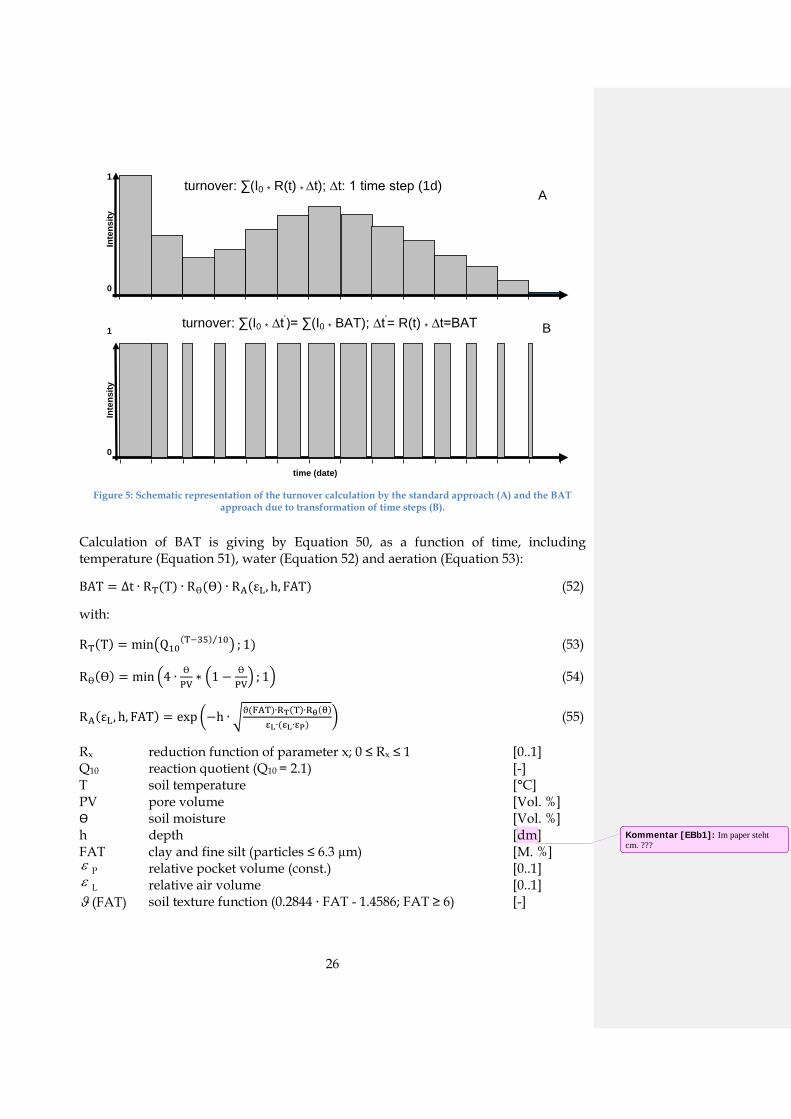
Description Biologic active time (BAT) is a concept that describes the impact of environmental conditions on biologic activity on soil organic matter (SOM) turnover (Franko et al. 1995). In a given time interval a certain biologic activity in a suboptimal environment will produce a specific turnover result. The same results occur when the time interval is split in BAT and non-BAT. During the BAT interval the microbial activity is only limited by the substrate, while during non-BAT there is no activity at all. For the calculation of the BAT interval, the effects of soil temperature, soil water and soil aeration are taken into account. The annual BAT sum is an important indicator for the potential turnover under the given conditions.

The scheme in Figure 5 demonstrates the principle how different intensities of uniform time steps (Figure 5 A) are transformed into time steps of different length and uniform intensity (Figure 5 B). The calculated turnover, symbolized by the bar area, will be the same for both approaches, anyway. In the latter case (B) the new calculated time step (∆t‘) is a product of the reduction function R(t) and the origin time step (∆t). In this case the non-BAT time step is represented as the blank space between the BAT bars (Figure 5 B).

BAT is calculated in daily time steps for the 3 top soil layers (0-3 dm) and distributed to the pore space classes used in CIPS (chapter CIPS).

26

Figure 5: Schematic representation of the turnover calculation by the standard approach (A) and the BAT

approach due to transformation of time steps (B).

Calculation of BAT is giving by Equation 50, as a function of time, including temperature (Equation 51), water (Equation 52) and aeration (Equation 53):

BAT = ∆t ∙ RT(T) ∙ RӨ(Ө) ∙ RA(εL, h, FAT) (52)

with:

RT(T) = min�Q10(T−35) 10⁄ � ; 1) (53)

RӨ(Ө) = min �4 ∙ ӨPV∗ �1 − Ө

PV� ; 1� (54)

RA(εL, h, FAT) = exp �−h ∙ �ϑ(FAT)∙RT(T)∙Rθ(θ)εL∙(εL∙εP)

� (55)

Rx reduction function of parameter x; 0 ≤ Rx ≤ 1 [0..1] Q10 reaction quotient (Q10 = 2.1) [-] T soil temperature [°C] PV pore volume [Vol. %] ϴ soil moisture [Vol. %] h depth [dm] FAT clay and fine silt (particles ≤ 6.3 µm) [M. %] ε P relative pocket volume (const.) [0..1] ε L relative air volume [0..1] ϑ (FAT) soil texture function (0.2844 ∙ FAT - 1.4586; FAT ≥ 6) [-]

0

1

Inte

nsity

time (date)

turnover: ∑(I0 * ∆t’)= ∑(I0 * BAT); ∆t‘= R(t) * ∆t=BAT

Inte

nsity

0

1 turnover: ∑(I0 * R(t) * ∆t); ∆t: 1 time step (1d)

B

A

Kommentar [EBb1]: Im paper steht cm. ???

27

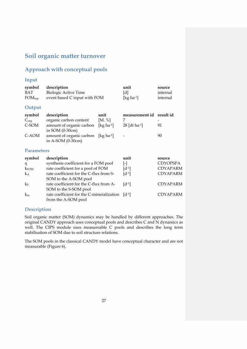
Soil organic matter turnover

Approach with conceptual pools

Input symbol description unit source BAT Biologic Active Time [d] internal FOMinp event based C input with FOM [kg ha-1] internal

Output symbol description unit measurement id result id Corg organic carbon content [M. %] 7 - C-SOM amount of organic carbon

in SOM (0-30cm) [kg ha-1] 28 [dt ha-1] 91

C-AOM amount of organic carbon in A-SOM (0-30cm)

[kg ha-1] - 90

Parameters symbol description unit source η synthesis coefficient for a FOM pool [-] CDYOPSPA kFOM rate coefficient for a pool of FOM [d-1] CDYAPARM kA rate coefficient for the C-flux from S-

SOM to the A-SOM pool [d-1] CDYAPARM

kS rate coefficient for the C-flux from A-SOM to the S-SOM pool

[d-1] CDYAPARM

km rate coefficient for the C-mineralization from the A-SOM pool

[d-1] CDYAPARM

Description Soil organic matter (SOM) dynamics may be handled by different approaches. The original CANDY approach uses conceptual pools and describes C and N dynamics as well. The CIPS module uses measureable C pools and describes the long term stabilisation of SOM due to soil structure relations.

The SOM pools in the classical CANDY model have conceptual character and are not measurable (Figure 6).

28

Figure 6: Conceptual pools and fluxes within the soil organic matter module in CANDY (description see text).

Soil organic matter is subdivided into four compartments: (1) fresh organic matter (FOM), (2) biological active soil organic matter (A-SOM or AOM), (3) stabilized soil organic matter (S-SOM or SSM) and (4) long term stabilized soil organic matter (LTS-SOM). All processes of the C turnover are formulated as first-order reactions (Franko et al. 1995). The model may handle up to six different FOM pools. A part of FOM is transferred into SOM. The relation of the SOM production to the FOM decay is described by the synthesis coefficient (η). The flux from FOM into A-SOM is called Crep. The A-SOM pool decays with a rate coefficient (kAOM). In addition to this, C loss to carbon dioxide, another flux from A-SOM to S-SOM, is modelled with the coefficient kSOM.

𝑑𝑑 𝐶𝐶𝐹𝐹𝐹𝐹𝐹𝐹(𝑡𝑡)𝑑𝑑𝑡𝑡

= 𝑘𝑘𝐹𝐹𝐹𝐹𝐹𝐹𝐹𝐹𝐹𝐹𝐹𝐹𝐹𝐹(𝑏𝑏) (56)

𝑑𝑑 𝐶𝐶𝑅𝑅𝑅𝑅𝑅𝑅(𝑡𝑡)𝑑𝑑𝑡𝑡

= 𝜂𝜂𝑘𝑘𝐹𝐹𝐹𝐹𝐹𝐹𝐹𝐹𝐹𝐹𝐹𝐹𝐹𝐹(𝑏𝑏) (57)

𝑑𝑑 𝐶𝐶𝐴𝐴𝐹𝐹𝐹𝐹(𝑡𝑡)𝑑𝑑𝑡𝑡

= 𝑑𝑑 𝐶𝐶𝑅𝑅𝑅𝑅𝑅𝑅(𝑡𝑡)𝑑𝑑𝑡𝑡

− (𝑘𝑘𝑚𝑚 + 𝑘𝑘𝑠𝑠)𝐹𝐹𝐴𝐴𝐹𝐹𝐹𝐹(𝑏𝑏) + 𝑘𝑘𝑙𝑙𝐹𝐹𝑇𝑇𝐹𝐹𝐹𝐹(𝑏𝑏) (58)

𝑑𝑑 𝐶𝐶𝑆𝑆𝐹𝐹𝐹𝐹(𝑡𝑡)𝑑𝑑𝑡𝑡

= 𝑘𝑘𝑠𝑠𝐹𝐹𝐴𝐴𝐹𝐹𝐹𝐹(𝑏𝑏) − 𝑘𝑘𝑙𝑙𝐹𝐹𝑇𝑇𝐹𝐹𝐹𝐹(𝑏𝑏) (59)

Cx carbon content of corresponding compartments of SOM [kg C ha-1] k rate coefficient [d-1] η dimensionless synthesis coefficient [-]

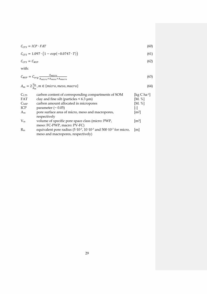
For the initialization of the CANDY model, the C amount of the LTS-SOM pool must be calculated. It is possible to choose from three different calculation methods: Fine particles after Körschens (Equation 58), clay content after Rühlmann (1999) (Equation 59) and particle surface after Puhlmann (Equation 60) and after Kuka (Equation 61) (Korschens 1980, Kuka 2005, Puhlmann et al. 2006).

29

𝐹𝐹𝐿𝐿𝑇𝑇𝑇𝑇 = 𝐼𝐼𝐹𝐹𝑀𝑀 ∙ 𝐹𝐹𝐵𝐵𝐵𝐵 (60)

𝐹𝐹𝐿𝐿𝑇𝑇𝑇𝑇 = 1.097 ∙ �1 − 𝑒𝑒𝑒𝑒𝑒𝑒(−0.0747 ∙ 𝐵𝐵)� (61)

𝐹𝐹𝐿𝐿𝑇𝑇𝑇𝑇 = 𝐹𝐹𝐹𝐹𝑀𝑀𝑀𝑀 (62)

with:

𝐹𝐹𝐹𝐹𝑀𝑀𝑀𝑀 = 𝐹𝐹𝑜𝑜𝑢𝑢𝑜𝑜𝐴𝐴𝑚𝑚𝑚𝑚𝑚𝑚𝑟𝑟𝑜𝑜

𝐴𝐴𝑚𝑚𝑚𝑚𝑚𝑚𝑟𝑟𝑜𝑜+𝐴𝐴𝑚𝑚𝑚𝑚𝑠𝑠𝑜𝑜+𝐴𝐴𝑚𝑚𝑚𝑚𝑚𝑚𝑟𝑟𝑜𝑜 (63)

𝐵𝐵𝑚𝑚 = 2 𝑉𝑉𝑚𝑚𝑇𝑇𝑚𝑚

,𝑚𝑚 ∈ {𝑚𝑚𝑏𝑏𝑚𝑚𝑏𝑏𝑏𝑏,𝑚𝑚𝑒𝑒𝑚𝑚𝑏𝑏,𝑚𝑚𝑚𝑚𝑚𝑚𝑏𝑏𝑏𝑏} (64)

CLTS carbon content of corresponding compartments of SOM [kg C ha-1] FAT clay and fine silt (particles < 6.3 μm) [M. %] CMIP carbon amount allocated in micropores [M. %] ICP parameter (~ 0.05) [-] Am pore surface area of micro, meso and macropores,

respectively [m2]

Vm volume of specific pore space class (micro: PWP, meso: FC-PWP, macro: PV-FC)

[m3]

Rm equivalent pore radius (5·10-7, 10·10-7 and 500·10-7 for micro, meso and macropores, respectively)

[m]

30

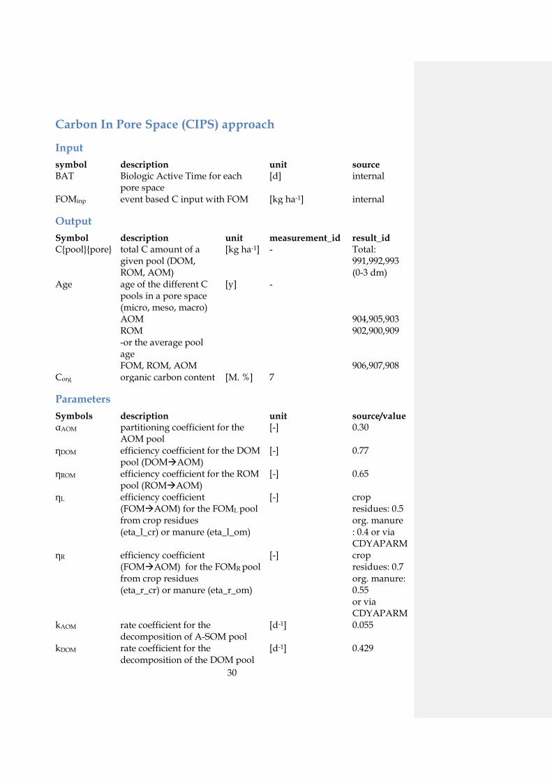
Carbon In Pore Space (CIPS) approach

Input symbol description unit source BAT Biologic Active Time for each

pore space [d] internal

FOMinp event based C input with FOM [kg ha-1] internal

Output Symbol description unit measurement_id result_id C{pool}{pore} total C amount of a

given pool (DOM, ROM, AOM)

[kg ha-1] - Total: 991,992,993 (0-3 dm)

Age age of the different C pools in a pore space (micro, meso, macro) AOM ROM -or the average pool age FOM, ROM, AOM

[y] - 904,905,903 902,900,909 906,907,908

Corg organic carbon content [M. %] 7

Parameters Symbols description unit source/value αAOM partitioning coefficient for the

AOM pool [-] 0.30

ηDOM efficiency coefficient for the DOM pool (DOMAOM)

[-] 0.77

ηROM efficiency coefficient for the ROM pool (ROMAOM)

[-] 0.65

ηL efficiency coefficient (FOMAOM) for the FOML pool from crop residues (eta_l_cr) or manure (eta_l_om)

[-] crop residues: 0.5 org. manure : 0.4 or via CDYAPARM

ηR efficiency coefficient (FOMAOM) for the FOMR pool from crop residues (eta_r_cr) or manure (eta_r_om)

[-] crop residues: 0.7 org. manure: 0.55 or via CDYAPARM

kAOM rate coefficient for the decomposition of A-SOM pool

[d-1] 0.055

kDOM rate coefficient for the decomposition of the DOM pool

[d-1] 0.429

31

kROM rate coefficient for the decomposition of the ROM pool

[d-1] 0.0011

kL rate coefficient for the decomposition of the FOML pool

[d-1] 0.25

kR rate coefficient for the decomposition of the FOMR pool

[d-1] 0.008

Description The CIPS model did overcome the necessity of empirical (conceptual) pools by taking into account soil structure effects and measurable pools (Figure 7 and Figure 8).

Following the usual convention that SOM is represented by the amount of organic carbon, and leaving the fresh organic matter (FOM) fraction as an external pool, the total amount of organic carbon (Corg) is represented by the sum of all soil borne carbon pools (Equation 63). Active organic matter (AOM) is the microbial biomass that is determined using the substrate induced respiration (SIR) method. Dissolved organic matter (DOM) can be measured by common methods, but is usually neglected during model initialisation.

Corg = AOM + ROM + DOM (65)

The general approach is characterized by:

• the division of SOM in qualitative pools on the basis of chemical measurability

• the dependence of the turnover conditions in terms of BAT (see chapter Biologic Active Time) from the location of SOM in pore space

• the structure dependent accessibility for microbial biomass The organic material enters the soil via the pool of fresh organic matter (FOM). The FOM pool is fed by plant residues and organic manure. According to its solubility in water and microbial degradability the FOM material is divided into:

• the soluble fraction (FOMS) • the insoluble part is separated according to its resistance against microbial

attacks in labile (FOML) resistant (FOMR)

The active organic matter (AOM) is considered as an equivalent to microbial biomass. It is the only living component acting as an engine of carbon turnover in soil.

Dissolved organic matter (DOM) is produced during the decay of other pools or may be imported with the soluble part of FOM.

Refractory organic matter (ROM) represents the insoluble product of microbial decay. This pool is considered as very resistant against microbial decomposition. Finally, all decay processes feed the pool of carbon dioxide (CO2).

32

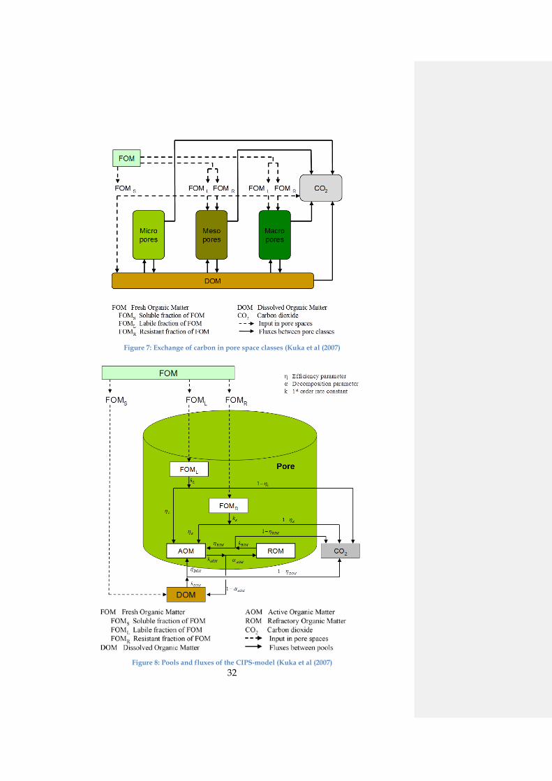
Figure 7: Exchange of carbon in pore space classes (Kuka et al (2007)

Figure 8: Pools and fluxes of the CIPS-model (Kuka et al (2007)

33

As shown in Figure 7 the pools are assigned to different pore space classes. According to their equivalent radius, soil pores are divided into three classes: micro-, meso- and macropores. The micropores represent the pore space of the permanent wilting point and the mesopores the pore space of available field capacity. The macropores correspond to the remaining pore space. The FOML and FOMR are only available for the AOM in meso- or macropores, because it is assumed that micropores are too small for organic matter particles. The FOMS directly feeds the DOM pool, which itself is available to all pore space classes providing a vehicle for matter exchange between them.

In every pore space class, equal pools are characterized with an identical set of parameters. Figure 8 shows the carbon fluxes between the carbon pools in each pore space class. With the decomposition of the FOML, FOMR, DOM and ROM pool carbon dioxide is produced and the biomass pool grows. The biomass pool itself decomposes into ROM and DOM. Equation 66 to Equation 69 describe the turnover dynamics for each pore space class with first-order kinetics and are based on the Biologic Active Time (BAT).

The total BAT of one time step is distributed to the single pore space classes according to their water saturation status (Kuka et al. 2007). If the soil water content is above field capacity it is assumed that all biological activity is located at the macropores. With reducing soil moisture, the biological activity is shared between two pore space classes. BAT is split between macro- and mesopore space if soil moisture is above the wilting point, and between meso- and micropore space if the soil moisture is further reduced below the wilting point. This principle follows the hypothesis, that biological activity needs free aeration as well as wetted surfaces. If one pore space class is completely drained, the biological activity in this class (BATlarger) is controlled by the part of surface that is still wet (Equation 64). This is represented by the volumetric water content of the next smaller pore space class (BATsmaller) (Equation 65).

BATlarger = VWVW+VA

∙ BATtot (66)

BATsmaller = VAVW+VA

∙ BATtot (67)

BATlarger see text above [d] BATsmaller see text above [d] VW water saturated volume of the smaller pore space class [Vol. %] VA air filled volume of the smaller pore space class [Vol. %] BATtot total Biologic Active Time [d]

As indicators for chemical pool stability, the k-values describe the matter breakdown. The efficiency parameters (η), as well as the decomposition parameter (αAOM) are used to split the matter flux between two destinations.

34

The AOM pool representing the microbial biomass is fed by the decomposition of the labile and resistant fraction of FOM (ηL, ηR) and by the inputs from ROM and DOM decay (Equation 66). The autolytic AOM decay (kAOM) is distributed into ROM (αAOM in Equation 67) and DOM (1- αAOM in Equation 68).

dAOMdt

= kLηLFOML + kRηRFOMR + kROMηROMROM + kDOMηDOMDOM − kAOMAOM (68)

The ROM pool is building up with products of the AOM pool decay (Equation 67). It decomposes itself and the matter flux is split into AOM ( ROMη in Equation 66) and CO2 (1− ROMη in Equation 69).

dROMdt

= kAOMαAOMAOM − kROMROM (69)

The DOM pool has an important function for the exchange of carbon between the different pore space classes. The AOM in all pore space classes may grow on this carbon source and during its decay it is feeding this pool as well (Equation 68).

dDOMdt

= FOMS + kAOm(1 − αAOM)AOM − kDOMDOM (70)

The first term of Equation 68 represents the direct input from the soluble fraction of FOM into the DOM pool. Further matter input results from the decomposition of AOM. The DOM is consumed by microbial biomass resulting in a growth of the AOM pool (ηDOM in Equation 66) with a partial decomposition to CO2 (1− ηDOM in Equation 69).

Equation 69 shows the sum of all mineralization fluxes into CO2 appearing during the growth of AOM.

dCO2dt

= kDOM(1 − ηDOM)DOM + kROM(1 − ηROM)ROM + kL(1 − FOML)FOML +kR(1 − ηR)FOMR (71)

Beside the basic pool dimensions the CIPS model also calculates the age (A) or the duration of the stay of carbon in these pools. The actual age of a pool is calculated in every time step as weighed means by pool contents (C), exports (E) and imports (I).

Ainew = 1 +

Aiold∙�Ci

old−Ei�+∑Aj∙IjCiold−Ei+∑Ej

(72)

To all external influxes (fertilization and plant residues) an age of zero is assigned. The initial age of all pools is read from the file cips_i.ini in the CANDY data dictionary. The file contains the initial values of the pool size (SIZE) as well as the pool age (AGE) of ROM, AOM and DOM.

If the model options include soil structure dynamics the results of that module are used for a re-distribution of the carbon on the pore classes. Depending on the structural changes the organic matter on the pore surface is transferred into a bigger (loosening) or smaller (compaction) pore class (Equation 71 and Equation 72).

35

∆Amic =

⎩⎨

⎧PWPold−PWPnew

PWPoldif PWPold > PWPnew

PWPold−PWPnewFKold−FKnew

if PWPold < PWPnew (73)

∆Ames =

⎩⎨

⎧FKold−FKnewFKold−PWPold

if FKold > FKnew

FKold−FKnewPVold−FKold

if FKold < FKnew

(74)

An alteration of the C pools arises from the changes of the surfaces in another pore class (Equation 73 to Equation 75).

∆Cmic = �−∆Amic ∙ Cmic if ∆Amic > 0

−∆Amic ∙ Cmes if ∆Amic < 0 (75)

∆Cmes =

⎩⎪⎨

⎪⎧

∆Amic ∙ Cmic if ∆Amic > 0

∆Amic ∙ Cmes if ∆Amic < 0

−∆Ames ∙ Cmes if ∆Ames > 0

−∆Ames ∙ Cmac if ∆Ames < 0

(76)

∆Cmac = �−∆Ames ∙ Cmes if ∆Ames > 0

−∆Ames ∙ Cmac if ∆Ames < 0 (77)

All pool sizes are calculated with Equation 76:

𝐹𝐹𝑛𝑛𝑢𝑢𝑛𝑛 = 𝐹𝐹𝑛𝑛𝑢𝑢𝑛𝑛 + ∆𝐹𝐹 (78)

36

N dynamics Input symbol description unit source N immission annual N deposition from

atmosphere [kg ha-1] CDY_FXDAT

N from fertilizer

from mineral fertilizer [kg ha-1] CDY_MADAT

Output symbol description unit measurement_id result_id N leaching downward N loss

via percolation through the lower boundary

[kg ha-1] - 102

gaseous N loss total gaseous N loss

[kg ha-1] - 106

N mineralization

Nmin transfer from/to SOM (mineralization: “+”, immobilization: “-“)

[kg ha-1] - 107

NH4-N ammonium nitrogen in specific soil layer

[kg ha-1] 3 -

NO3-N nitrate nitrogen in specific soil layer

[kg ha-1] 1 -

NH4 loss gaseous

ammonia volatilization

[kg ha-1] - 123

N2O emission N2O-N emission [kg ha-1] 75 997

Parameters symbol description unit source table N_IM_BEW immission for cropped land [-] CNDAPARM N_IM_SOM immission for summer

season [-] CNDAPARM

SBA parameterset

decision support system for nitrogen fertilization (ger.: Stickstoffbedarfs-Analyse)

[-]

CNRmic C/N ratio of microbial biomass (standard: 8.5)

[-] CNDAPARM

37

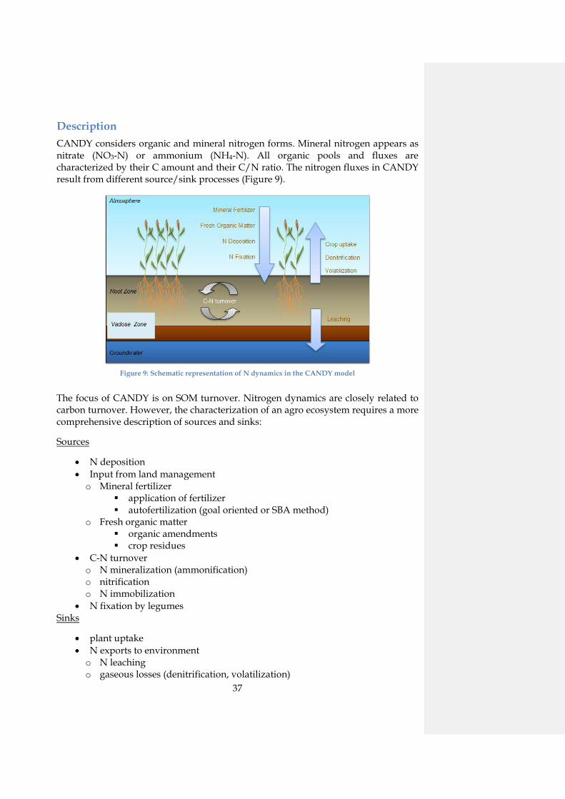
Description CANDY considers organic and mineral nitrogen forms. Mineral nitrogen appears as nitrate (NO3-N) or ammonium (NH4-N). All organic pools and fluxes are characterized by their C amount and their C/N ratio. The nitrogen fluxes in CANDY result from different source/sink processes (Figure 9).

Figure 9: Schematic representation of N dynamics in the CANDY model

The focus of CANDY is on SOM turnover. Nitrogen dynamics are closely related to carbon turnover. However, the characterization of an agro ecosystem requires a more comprehensive description of sources and sinks:

Sources

• N deposition • Input from land management o Mineral fertilizer

application of fertilizer autofertilization (goal oriented or SBA method)

o Fresh organic matter organic amendments crop residues

• C-N turnover o N mineralization (ammonification) o nitrification o N immobilization

• N fixation by legumes Sinks

• plant uptake • N exports to environment o N leaching o gaseous losses (denitrification, volatilization)

38

Nitrogen Sources

N deposition N deposition has to be defined with the basic data as mean annual value. This value will be modified internally according to the actual season (summer: 120 < Julian day < 304) and the vegetation cover (yes/no) in case that the following parameter values have been defined in the CNDAPARM table:

N_IM_BEW (immission for cropped land) standard: 0.17

N_IM_SOM (immission for summer season) standard: 0.71

In the case that the parameters are not defined (Null or 0) an equal distribution of N immission over the whole year will be assumed.

Input from land management

Application of fertilizer The management data (CDY_MADAT) contain the amount and application date of mineral nitrogen as well as the fertilizer form which is used to distribute the total N into NO3 and NH4 pools on the soil surface.

Goal oriented fertilization If the management data contain negative values for an event of N fertilization, the model uses the absolute value as nitrogen goal. In this case, the actual amount of applied fertilizer is the difference between that goal and the mineral nitrogen store in the rooted soil profile.

Autofertilization SBA method (german: Stickstoff-Bedarfs-Analyse)

For scenario simulations there is often no information available about the actual fertilization rates. In order to simulate an appropriate farming level it is possible to calculate the required fertilizer N from the mineral N amount in the soil and the rules that are used in advisory service for good farming practice. In CANDY the user may apply the rules of the SBA method. In this case it is necessary to specify the dates of N application and code the amount of N with -999.

There may be up to four application dates. The first two dates are reserved to the first fertilization event, since N may be split between these two dates in case of high doses. The next two fertilization dates belong to the second and a third fertilization event. Only for the first event the amount of N fertilizer is related to the soil storage of mineral nitrogen at that time. N amounts for the second and third event are based on table values.

39

Organic amendments Any fresh organic matter (FOM) pool may include organic bound nitrogen as well as inorganic nitrogen. Therefore, the parameter set contains two different C/N ratios.

CNR: Corg/Norg

CNR_alt: Corg/(Norg+Nmin)

A third (redundant) parameter describes the relation between mineral and organic (MOR) bound N.

MOR: Nmin/Norg

or

MOR: (CNR/CNR_alt) - 1

Mineralisation / Immobilisation During FOM decomposition N is released into the ammonia pool according to the C/N ratio of the FOM pool. The FOM decomposition goes along with a microbial growth where the C reproduction flux is controlled by the η parameter of the FOM. The required N for this growth, defined by CNRmic, is taken from the mineral N – first from ammonia then from nitrate. If not enough mineral nitrogen is available, the decomposition rate is reduced in order to avoid negative Nmin.

N fixation by legume crop Symbiotic N fixation may be an important nitrogen source especially for semi-natural systems or in case of organic farming. The process of N fixation is controlled by crop parameters containing the uptake rate from soil and the time dependence of the development of symbiotic fixation potential. After harvest the root system contains a remarkable amount of nitrogen that is handled like mineral nitrogen and distributed over the whole soil profile instead of staying only in the top soil.

Nitrogen sinks

Plant uptake Plant uptake is the most important sink for agroecosystems because this flux controls yield and product quality. A detailed description is given in the crop module (see Crop Module).

N losses

Leaching NO3-N will be leached downward with the water percolation. It is assumed that only the water in meso and macropores is moving. According to this, the nitrogen

40

dissolved in the water of the micropores is not leached. After each leaching event the nitrogen is redistributed between the complete pore systems of each soil layer.

The leached nitrogen (NL) from one soil layer is calculated according to Equation 77.

NL = NNO3 ∙ �1 − D ∙ PWPFC

� ∙ PӨ0

(79)

NL leached nitrogen [kg ha-1] PWP water content at permanent wilting point [Vol. %] FC water content at field capacity [Vol. %] P water percolation [mm d-1] D calibration parameter DISP_KF in CNDAPARM [-] Ө0 initial water content [Vol. %] NNO3 amount of nitrate N in the calculation layer [kg ha-1]

Gaseous Losses Ammonia volatilization is calculated at the application event of organic amendments. If no soil tillage is registered during the next 3 days, 20% of the applied NH4-N is taken from the soil as volatized.

Gaseous losses from nitrate N are calculated as a result of anaerobic turnover. Whereas the temperature impact (rT) on the anaerobic turnover is considered the same as for the BAT calculation. The following reduction function (RӨ) is applied for the soil moisture impact (Equation 78):

𝑅𝑅Ө = �Ө+0.627∙𝐹𝐹𝐶𝐶−0.0267∙𝑀𝑀𝑉𝑉∙𝐹𝐹𝐶𝐶1.627∙𝐹𝐹𝐶𝐶−0.0267∙𝑀𝑀𝑉𝑉∙𝐹𝐹𝐶𝐶

(80)

RӨ reduction function for soil moisture impact on denitrification

[-]

FC water content at field capacity [Vol. %] PV soil pore volume [Vol. %] Ө water content [Vol. %]

The amount of volatized nitrogen (Ndeni) is dependent on the rate constant kdeni, the size of the NO3 pool (NNO3), and the amount of carbon in the AOM pool (CAOM). The denitrification rate is limited according to the parameter MAXDENI in CNDAPARM.

𝑁𝑁𝑑𝑑𝑢𝑢𝑛𝑛𝑑𝑑 = 𝑀𝑀𝐼𝐼𝑁𝑁�𝑀𝑀𝐵𝐵𝑀𝑀𝐵𝐵𝑀𝑀𝑁𝑁𝐼𝐼,𝑘𝑘𝑑𝑑𝑢𝑢𝑛𝑛𝑑𝑑 ∙ 𝑅𝑅Ө ∙ 𝑅𝑅𝑇𝑇 ∙ 𝑁𝑁𝑁𝑁𝐹𝐹3 ∙ 𝐹𝐹𝐴𝐴𝐹𝐹𝐹𝐹� (81)

Ndeni denitrificated nitrogen [kg ha-1] kdeni constant denitrification factor [-] RӨ reduction function for soil moisture impact on

denitrification [-]

RT reduction function for soil temperature impact on denitrification

[-]

MAXDENI maximum amount of denitrification [kg ha-1]

41

CAOM total C amount of active organic matter [kg ha-1] NNO3 amount of nitrate N in the calculation layer [kg ha-1]

Following the approaches of Parton the N flux from denitrification is split between N2 and N2O (Equation 80 to Equation 83) (Parton et al. 1996). This partitioning is controlled by factors depending on the water filled pore space (fwfps), the CO2 production rate PCO2 (fCO2) and the nitrate concentration CNO3 (fNO3).

fwfps = 1.4

13� 1713(2.2∙wfps)�

(82)

with

𝑤𝑤𝑓𝑓𝑒𝑒𝑚𝑚 = 𝜃𝜃𝑀𝑀𝑉𝑉

(83)

fCO2 = 13 +30.78∙arctan�π∙0.07∙�PCO2−13��

π (84)

fNO3 = 25 ∙ �1 − �0.5 +arctan�π∙0.01∙�CNO3−190��

π�� (85)

The partitioning coefficient RN2/N2O is calculated from the product of f_wfps and the geometric mean of the factors for NO3 and CO2 effects (Equation 84).

𝑅𝑅𝑁𝑁2/𝑁𝑁2𝐹𝐹 = 𝑓𝑓𝑛𝑛𝑤𝑤𝑢𝑢𝑠𝑠 ∙ ��𝑓𝑓𝑁𝑁𝐹𝐹3 ∙ 𝑓𝑓𝐶𝐶𝐹𝐹2� (86)

Finally the resulting N2O flux (NN2O) is calculated with Equation 85.

𝑁𝑁𝑁𝑁2𝐹𝐹 = 𝑁𝑁𝑑𝑑𝑚𝑚𝑛𝑛𝑚𝑚1+𝑇𝑇𝑁𝑁2/𝑁𝑁2𝐹𝐹

(87)

42

Crop module

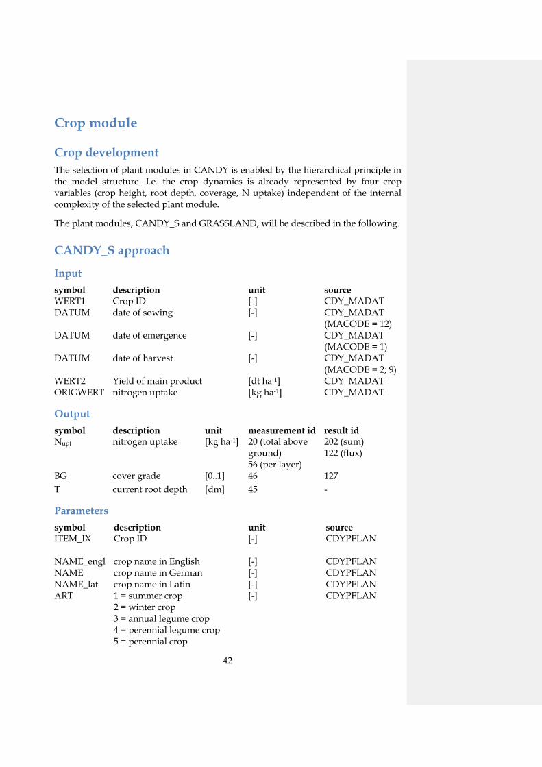
Crop development The selection of plant modules in CANDY is enabled by the hierarchical principle in the model structure. I.e. the crop dynamics is already represented by four crop variables (crop height, root depth, coverage, N uptake) independent of the internal complexity of the selected plant module.

The plant modules, CANDY_S and GRASSLAND, will be described in the following.

CANDY_S approach

Input symbol description unit source WERT1 Crop ID [-] CDY_MADAT DATUM date of sowing [-] CDY_MADAT

(MACODE = 12) DATUM date of emergence [-] CDY_MADAT

(MACODE = 1) DATUM date of harvest [-] CDY_MADAT

(MACODE = 2; 9) WERT2 Yield of main product [dt ha-1] CDY_MADAT ORIGWERT nitrogen uptake [kg ha-1] CDY_MADAT

Output symbol description unit measurement id result id Nupt nitrogen uptake [kg ha-1] 20 (total above

ground) 56 (per layer)

202 (sum) 122 (flux)

BG cover grade [0..1] 46 127 T current root depth [dm] 45 -

Parameters symbol description unit source ITEM_IX Crop ID [-] CDYPFLAN NAME_engl crop name in English [-] CDYPFLAN NAME crop name in German [-] CDYPFLAN NAME_lat crop name in Latin [-] CDYPFLAN ART 1 = summer crop

2 = winter crop 3 = annual legume crop 4 = perennial legume crop 5 = perennial crop

[-] CDYPFLAN

43

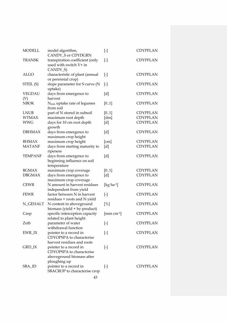
MODELL model algorithm, CANDY_S or CDYDGRN

[-] CDYPFLAN

TRANSK transpiration coefficient (only used with switch V+ in CANDY_S)

[-] CDYPFLAN

ALGO characteristic of plant (annual or perennial crop)

[-] CDYPFLAN

STEIL (S) slope parameter for S curve (N uptake)

[-] CDYPFLAN

VEGDAU (V)

days from emergence to harvest

[d] CDYPFLAN

NBOK Nmin uptake rate of legumes from soil

[0..1] CDYPFLAN

LNUB part of N stored in subsoil [0..1] CDYPFLAN WTMAX maximum root depth [dm] CDYPFLAN WWG days for 10 cm root depth

growth [d] CDYPFLAN

DBHMAX days from emergence to maximum crop height

[d] CDYPFLAN

BHMAX maximum crop height [cm] CDYPFLAN MATANF days from starting maturity to

ripeness [d] CDYPFLAN

TEMPANF days from emergence to beginning influence on soil temperature

[d] CDYPFLAN

BGMAX maximum crop coverage [0..1] CDYPFLAN DBGMAX days from emergence to

maximum crop coverage [d] CDYPFLAN

CEWR N amount in harvest residues independent from yield

[kg ha-1] CDYPFLAN

FEWR factor between N in harvest residues + roots and N yield

[-] CDYPFLAN

N_GEHALT N content in aboveground biomass (yield + by-product)

[%] CDYPFLAN

Czep specific interception capacity related to plant height

[mm cm-1] CDYPFLAN

Zetb parameter of water withdrawal function

[-] CDYPFLAN

EWR_IX pointer to a record in CDYOPSPA to characterise harvest residues and roots

[-] CDYPFLAN

GRD_IX pointer to a record in CDYOPSPA to characterise aboveground biomass after ploughing up

[-] CDYPFLAN

SBA_ID pointer to a record in SBACROP to characterise crop

[-] CDYPFLAN

44

for automatic fertilization HI relation of by-product to main

product [-] CDYPFLAN

KOP_IX pointer to a record in CDYOPSPA to characterise by-product

[-] CDYPFLAN

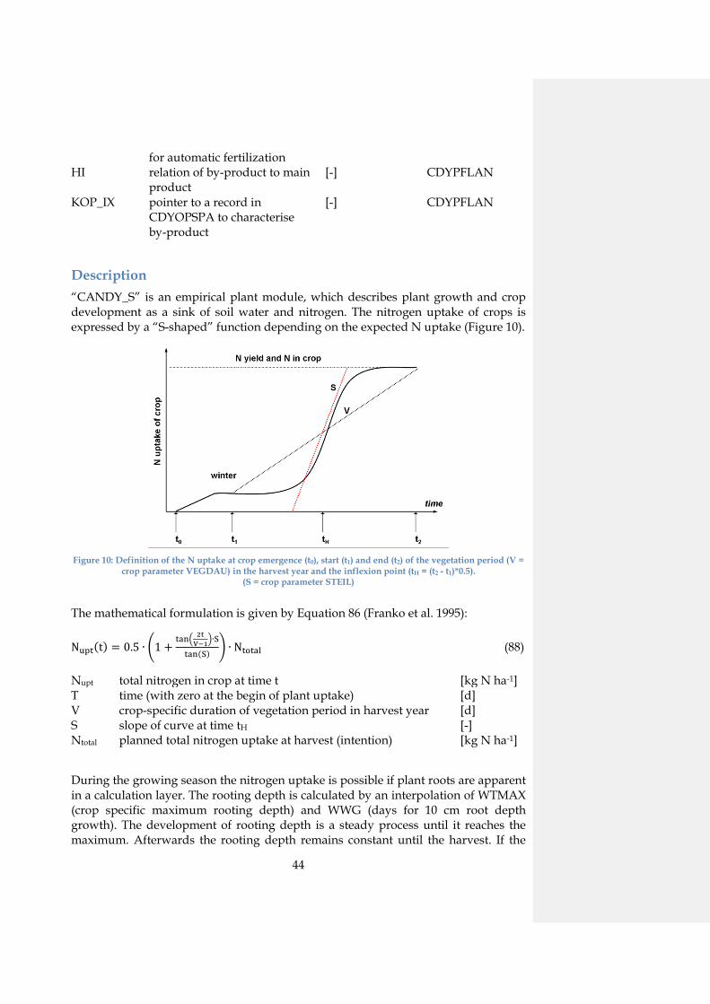
Description “CANDY_S” is an empirical plant module, which describes plant growth and crop development as a sink of soil water and nitrogen. The nitrogen uptake of crops is expressed by a “S-shaped” function depending on the expected N uptake (Figure 10).

Figure 10: Definition of the N uptake at crop emergence (t0), start (t1) and end (t2) of the vegetation period (V =

crop parameter VEGDAU) in the harvest year and the inflexion point (tH = (t2 - t1)*0.5). (S = crop parameter STEIL)

The mathematical formulation is given by Equation 86 (Franko et al. 1995):

Nupt(t) = 0.5 ∙ �1 +tan� 2t

V−1�∙S

tan(S) � ∙ Ntotal (88)

Nupt total nitrogen in crop at time t [kg N ha-1] T time (with zero at the begin of plant uptake) [d] V crop-specific duration of vegetation period in harvest year [d] S slope of curve at time tH [-] Ntotal planned total nitrogen uptake at harvest (intention) [kg N ha-1]

During the growing season the nitrogen uptake is possible if plant roots are apparent in a calculation layer. The rooting depth is calculated by an interpolation of WTMAX (crop specific maximum rooting depth) and WWG (days for 10 cm root depth growth). The development of rooting depth is a steady process until it reaches the maximum. Afterwards the rooting depth remains constant until the harvest. If the

45

soil moisture reaches permanent wilting point (PWP), the N uptake of the plant is stopped.

A part of the total N uptake returns to the soil as harvest residues and roots (Equation 87).

Nres = Nupt∙FEWR∙CEWR1+FWER

= CEWR + Nyield ∙ FEWR (89)

Nres N amount from harvest residues and roots [kg N ha-1] Nupt total N in crop (yield + by-product + roots and residues) [kg N ha-1] Nyield N amount in main and by-product [kg N ha-1] CEWR N amount in harvest residues independent from yield [kg N ha-1] FEWR factor between N in harvest residues and roots and N yield [-]

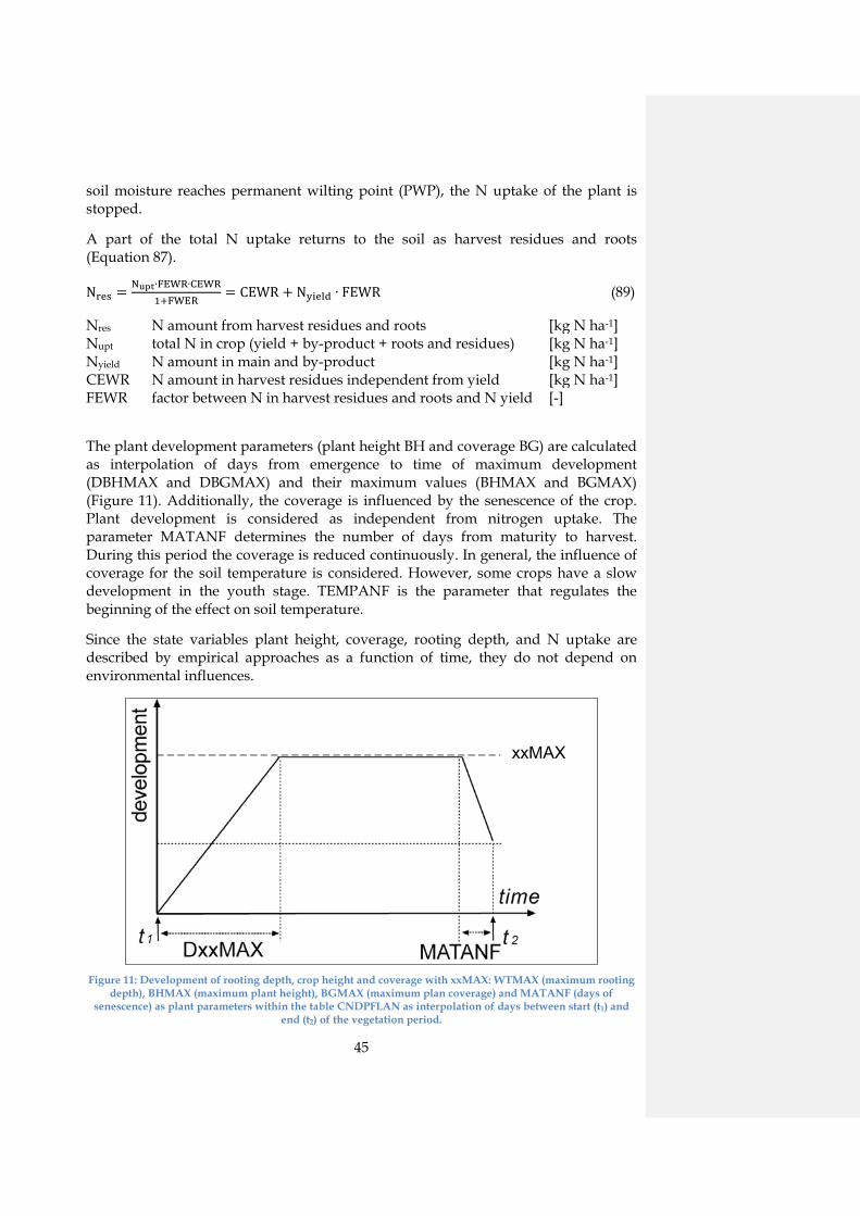
The plant development parameters (plant height BH and coverage BG) are calculated as interpolation of days from emergence to time of maximum development (DBHMAX and DBGMAX) and their maximum values (BHMAX and BGMAX) (Figure 11). Additionally, the coverage is influenced by the senescence of the crop. Plant development is considered as independent from nitrogen uptake. The parameter MATANF determines the number of days from maturity to harvest. During this period the coverage is reduced continuously. In general, the influence of coverage for the soil temperature is considered. However, some crops have a slow development in the youth stage. TEMPANF is the parameter that regulates the beginning of the effect on soil temperature.

Since the state variables plant height, coverage, rooting depth, and N uptake are described by empirical approaches as a function of time, they do not depend on environmental influences.

Figure 11: Development of rooting depth, crop height and coverage with xxMAX: WTMAX (maximum rooting

depth), BHMAX (maximum plant height), BGMAX (maximum plan coverage) and MATANF (days of senescence) as plant parameters within the table CNDPFLAN as interpolation of days between start (t1) and

end (t2) of the vegetation period.

xxMAX

46

Legumes

Input See crop module

Output See crop module

Parameter See crop module

Description The principle of CANDY_S represents the base for the modelling of legumes and grassland as well. Further parameters complete the calculation for these plants.

The parameter ART defines a plant type (ART=3: annual legume crop, ART=4: perennial legume crop). Additional to the organic bound N amount of the residues, CANDY considers a certain amount of inorganic N that is equally deposited in the subsoil (Equation 88).

Nres = Nres ∙ (1 − LNUB) (90)

LNUB part of N stored in subsoil [0..1]

The fixation of atmospheric nitrogen is given by Equation 89 and Equation 90.

Nsym = Ndem ∙ (1 − NBOK) (91)

Nsoil_up = Ndem − Nsym (92)

Nsym daily N uptake from symbiotic fixation [kg N ha-1] Ndem daily N demand [kg N ha-1] Nsoil_up daily N uptake from soil Nmin pool [kg N ha-1] NBOK part of N uptake from soil Nmin pool [0..1]

47

Permanent Grasslands

Input symbol description unit source LTEM daily air temperature [°C] CDY_CLDAT ETa actual evapotranspiration [mm] internal iLCU increase of livestock units CDYMADAT

(MACODE = 10) dLCU decrease of livestock units CDYMADAT

(MACODE = 11)

Output See crop module

Parameters symbol description unit source TRANSKO transpiration coefficient [kg] CDYGRAS TS1 threshold 1 of temperature sum [°C] CDYGRAS TS2 threshold 2 of temperature sum [°C] CDYGRAS TK_MIN minimum of transpiration

coefficient [kg mm-1] CDYGRAS

TK_MAX maximum of transpiration coefficient

[kg mm-1] CDYGRAS

C_INP carbon-FOM input from animal faeces for 1 animal unit

[kg ha-1 d.1] CDYLIVES

OD_ID item_ix of OM from animal faeces [-] CDYLIVES N_UPT nitrogen uptake from plant biomass

for 1 animal unit [kg ha-1 d-1] CDYLIVES

Description The grassland is managed by several cuts over the year with an optional grazing from livestock. In addition, grassland is characterised by long vegetation duration. The N uptake of the crop is controlled by the temperature sum and the actual evapotranspiration. If air temperature is above 4°C the daily N uptake is calculated by Equation 91 to Equation 95.

TS = TS + LTEM − 4 (93)

TRANSKO = TKmax; TS ≤ TS1 (94)

TRANSKO = TKmin + (TKmax − TKmin ∙ N) ∙ TS2−TSTS2−TS1

; TS1 < TS < TS2 (95)

TRANSKO = TKmin; TS ≥ TS2 (96)

Nup = Nup + TRANSKO ∙ ETa (97)

48

TS temperature sum [-] LTEM daily air temperature [°C] TRANSKO transpiration coefficient [kg mm-1] TS1 threshold 1 of temperature sum [°C] TS2 threshold 2 of temperature sum [°C] TKmin minimum of transpiration coefficient [kg mm-1] TKmax maximum of transpiration coefficient [kg mm-1] Nup N uptake of plant [kg ha-1] ETa actual evapotranspiration [mm]

If the number of animal units is not null the biomass N pool is reduced due to grazing with the amount of N uptake by animals given in the parameter N_UPT (Equation 96 and Equation 97). Animal faeces are treated as organic amendments (Equation 98). The specific addition of organic matter is described by the parameters OD_ID (quality) and C_INP (quantity). Animal units that are defined in the table CDYLIVES can be located and relocated to/from the grassland as a management activity.

NAU = NAU + ∆NAU (98)

NGR = NAU + N_UPT (99)

COA = NAU + N_INP (100)

NAU number of animal units [-] NGR N uptake by grazing animals [kg ha-1] COA carbon flux to soil with fresh organic matter from animal

faeces [kg ha-1 d-1]

N_UPT specific N uptake (parameter) [kg ha-1 d-1] C_INP specific C input from faeces [kg ha-1 d-1]

V

Literature Brooks, R. H., and A. T. Corey (1964). Hydraulic properties of porous media. Hydrolgical Paper. Colorado State University, Fort Collins. 3.

Franko, U., B. Oelschlägel and S. Schenk (1995). "Simulation of temperature-, water-and nitrogen dynamics using the model CANDY." Ecological Modelling 81(1): 213-222.

Glugla, G. (1969). "Berechnungsverfahren zur Ermittlung des aktuellen Wassergehalts und Gravitationswasserabflusses im Boden." Archives of Agronomy and Soil Science 13(4): 371-376.

Koitzsch, R. (1990). "Bodenfeuchte-und Verdunstungsmodell BOWA." Interner Bericht. FZ Müncheberg. Müncheberg.

Koitzsch, R. and R. Günther (1990). "Modell zur ganzjährigen Simulation der Verdunstung und der Bodenfeuchte landwirtschaftlicher Nutzflächen mit und ohne Bewuchs." Archiv für Acker-und Pflanzenbau und Bodenkunde 34(12): 803-810.

Korschens, M. (1980). "Beziehungen zwischen Feinanteil, Ct-und Nt-Gehalt des Bodens." Archiv fur Acker-und Pflanzenbau und Bodenkunde.

Kuka, K. (2005). Modellierung des Kohlenstoffhaushaltes in Ackerböden auf der Grundlage bodenstrukturabhängiger Umsatzprozesse, UFZ-Umweltforschungszentrum Leipzig-Halle GmbH.

Kuka, K., U. Franko and J. Rühlmann (2007). "Modelling the impact of pore space distribution on carbon turnover." Ecological Modelling 208(2–4): 295-306.

Lieberoth, I. (1982). "Bodenkunde." VEB Deutscher Landwirtschaftsverlag, Berlin: 432.

Nemes, A., J. Wösten, A. Lilly and J. O. Voshaar (1999). "Evaluation of different procedures to interpolate particle-size distributions to achieve compatibility within soil databases." Geoderma 90(3): 187-202.

Parton, W., A. Mosier, D. Ojima, D. Valentine, D. Schimel, K. Weier and A. E. Kulmala (1996). "Generalized model for N2 and N2O production from nitrification and denitrification." Global biogeochemical cycles 10(3): 401-412.

Puhlmann, M., K. Kuka and U. Franko (2006). "Comparison of methods for the estimation of inert carbon suitable for initialisation of the CANDY model." Nutrient Cycling in Agroecosystems 74(3): 295-304.

Rawls, W. J. and D. L. Brakensiek (1985). Prediction of soil water properties for hydrologic modeling. Watershed management in the eighties, American society of civil engineers.

VI

Ruehlmann, J. and M. Körschens (2009). "Calculating the Effect of Soil Organic Matter Concentration on Soil Bulk Density." Soil Science Society of America Journal 73(3): 876-885.

Rühlmann, J. (1999). "A new approach to estimating the pool of stable organic matter in soil using data from long-term field experiments." Plant and Soil 213(1-2): 149-160.

Rühlmann, J., M. Körschens and J. Graefe (2006). "A new approach to calculate the particle density of soils considering properties of the soil organic matter and the mineral matrix." Geoderma 130(3): 272-283.

Schaaf, T. (1998). Integration von Modellansätzen zur Bodenbearbeitung und Düngung in den Baukasten für Stickstoffsimulationsmodelle EXPERT-N, ZADI.

Suckow, F. (1987). Ein Modell zur Berechnung der Bodentemperatur unter Brache und unter Pflanzenbestand.

Turc, L. (1961). "Estimation of irrigation water requirements, potential evapotranspiration: a simple climatic formula evolved up to date." Ann Agron 12(1): 13-49.

Van Genuchten, M. T. (1980). "A closed-form equation for predicting the hydraulic conductivity of unsaturated soils." Soil science society of America journal 44(5): 892-898.

Vereecken, H., J. Maes, J. Feyen and P. Darius (1989). "Estimating the soil moisture retention characteristic from texture, bulk density, and carbon content." Soil science 148(6): 389-403.

Zacharias, S. and G. Wessolek (2007). "Excluding organic matter content from pedotransfer predictors of soil water retention." Soil Science Society of America Journal 71(1): 43-50.