Embed Size (px)
Citation preview

Canonical Least Squares Clustering onSparse Medical Data
Igor GitmanMachine Learning Department
Carnegie Mellon [email protected]
Jieshi ChenAuton Lab
Carnegie Mellon [email protected]
Artur DubrawskiAuton Lab
Carnegie Mellon [email protected]
Abstract
We explore different applications of Canonical Least Squares (CLS) clustering ona corpus of sparse medical claims from a particular health insurance provider. Wefind that there are several reasons why most conclusions based on CLS clustersmight be misleading, especially when the data is significantly sparse. We illustratethese findings by performing a number of synthetic experiments with the mostfocus on the sparsity issue since it has not been explored in the literature before.Based on the insights from the synthetic experiments we show how CLS clusteringcan be potentially applied to identify hospital peer-groups: hospitals that sharesimilar operational characteristics. In addition we demonstrate that CLS clusteringcan be used to improve prediction results for the patients length of stay in thehospitals.
1 Introduction
Data clustering can be useful in various applications. These applications can be roughly divided intotwo groups: data analysis applications and prediction applications. The goal of the first group is tofind some new properties of the data by examining obtained clusterings. The goal of the second groupis to improve results of prediction models by adding cluster labels as features. Regardless of theapplication, the goal of the clustering algorithm is to find groups of objects that are similar accordingto some predefined criteria. One popular choice of similarity criteria is L2 distance in feature space.In that case such well-known algorithms as k-means [21] or some form of hierarchical clustering [23]can be used. When feature space contains some dependent or target variable (e.g. produced bylinear combination of other features), it might be reasonable to seek the groups of objects that havethe same relation between dependent and independent variables (e.g. the same linear regressioncoefficients). In that case, some form of cluster-wise linear regression (CLR) can be used, e.g. [27]or [9]. When there are multiple dependent variables and one seeks to find clusters with differentcorrelation patterns, canonical correlation analysis (CCA) clustering [10] can be applied. Recently,there has been proposed a canonical least squares (CLS) clustering method [18] that achieves similargoal to CCA, but is more robust and its results usually have better interpretations.
In this paper we explore potential applications of CLS to a corpus of medical claims of patients froma particular health insurance provider. For each claim there are 87 different fields characterizing thatclaim. These fields include: patients id, claim id, provider id, admittance/discharging dates, patientage, gender, diagnosis related group (DRG) and other. We first preprocess this data filtering outliersand not useful features and then produce two different aggregations: claim-level data (with eachobject corresponding to one claim) and hospital-level data (with each object corresponding to oneprovider, which is usually a hospital). More details about dataset and feature selection/aggregationprocesses are given in section 3.
One notable feature extracted from this data is patient length of stay in the hospital (or average lengthof stay for a certain DRG in case of the hospital-level data). This feature can be used as a measure

of quality of care for the hospital or claim. There are many business applications that could benefitfrom finding groups of claims or hospitals that have similar correlation patterns with quality of care.One example of such application is finding comparable groups of hospital or “peer groups” that havesimilar operational characteristics and similar length of stay dependence on those characteristics.These groups can then be used to assess hospitals performance fairly by comparing them with eachother only inside their peer group and not across all hospitals. On a claim level, finding clusters thathave similar correlation patterns can be useful for prediction purposes. It is reasonable to assume thatdifferent claims are not homogeneous in terms of their correlation with length of stay. For example,some patients can have different reactions to certain diseases or types of treatment. Thus, identifyingregression-based clusters and using different regression models for them could potentially improvethe prediction accuracy for a length of stay.
In this paper we demonstrate applications of CLS towards these two goals: correlation-based dataanalysis and improvement of prediction results. We start by reviewing the related work for bothof these problems in section 2. We describe dataset used in this paper in more details in section 3and give a brief introduction into CLS algorithm in section 4. In section 5 we describe a numberof preliminary experiments that lead us to believe that a straightforward application of CLS to aclaim-level data analysis is likely to give misleading results. We identify 3 main problems:
1. Standard metrics evaluating CLS performance overestimate goodness of linear fit to thedata.
2. CLS is prone to finding non-intuitive correlations that only exists in the data by chance.3. Applying CLS on sparse data is complicated since there are multiple good solutions, with
some extreme cases when CLS problem becomes ill-defined.
The first two problems were mentioned in the literature before in the work of Brusco et al [5] andVicari et al [28]. In this paper we give a few more intuitive examples illustrating the issues as well asprovide more general and practical formulations of possible solutions in sections 6.1 and 6.2. Thesparsity problem has not been explored before and thus we give a detailed analysis of this problemby running a series of synthetic experiments in section 6.3. In section 7.1 we demonstrate how CLScan be used to improve traditional methods of hospital peer-groups creation. Finally, in section 7.2we introduce two novel approaches to prediction with regression-based clustering: predictive CLSwhich combines CLS objective with k-means and uses a separate classification model to predict CLSlabels at test time; and constrained CLS, which uses a user-defined set of constraints on some featuresthat are known at test time and thus could be used to derive test labels. We show that these methodsperform better than other models, such as linear regression, random forest [4] and k-plane: a similarregression-based clustering algorithm proposed in [22]. We summarize and conclude the paper insection 8.
2 Related work
2.1 Interpretability analysis
When there is only one dependent variable, CLS is equivalent to CLR, proposed by Spath in 1979 [27]which has been extensively studied in the literature. Hennig [12] explores the problem of identifiabilityof linear regression mixtures and proves a set of necessary conditions. In this work we show withsimple examples and experiments that strong sparsity can also lead to non-identifiable mixtures whichwas not studied in the original work by Hennig. Although we do not provide any complete theoreticalresults it is a potential direction of future research.
The problem of CLR overestimating the goodness of linear fit was first observed by Brusco et al [5].The authors argue that even when target variable is generated independently from other features, CLRwill find a solution with surprisingly good coefficient of determination (R2) and mean squared error(MSE). They show that MSE comprises of 2 terms: within-cluster distances and between-clusterdistances. Since CLR finds regression coefficients and clusters simultaneously, it might optimizebetween-cluster distance only (by grouping objects with similar target values), ignoring within-clustercorrelations. The authors propose a different metric (based on hypothesis testing) to assess theperformance of CLR adjusted for such a good behaviour when features and targets are independent.We reinforce the analysis of Brusco et al [5] by providing exact theoretical solution for the uniformlydistributed targets. We also suggest a different adjusted metric which only requires running CLR 2
2
times and thus is exponentially faster to compute in the general CLS case when the dimension oftarget variables is greater than 1.
Vicari et al [28] expands on the work of Brusco et al [5] showing that since CLR doesn’t distinguishbetween within-cluster and between-cluster distances it can converge to a very non-intuitive solutions.The authors devise an algorithm that has different models for relations within one cluster and relationsbetween different clusters. The final algorithm can be seen as combining CLR objective with k-meansobjective which has also been explored by [6], [22], [8]. We reinforce these observations with simpleexamples and provide a general regularized reformulation of CLS, with k-means regularization beinga particular instance.
2.2 Hospital peer-groups
The traditional approaches to finding hospital peer groups usually utilize standard clustering tech-niques. Klastorin [17] is using hierarchical clustering to identify peer groups. Alexander et al [1]suggests to use k-means and factor analysis instead which provides a better way to understand howgood the given clustering is. These techniques were tested by Zodet and Clark [31], MacNabb [20]and Kang et al [16] on the hospital data from the state of Michigan, Canada and South Korea corre-spondingly. Another approach to defining hospital peer groups was developed by Byrne et al [7]. Theauthors suggested that peer groups might not be mutually exclusive and created a nearest neighborsbased algorithm for identifying the peer groups centered at each hospital.
2.3 Prediction
There are multiple approaches on how to use regression-based clustering for prediction. Kang etal [15] suggests to use fuzzy clustering with Dirichlet prior so that it would be possible to obtainlabels at test time. Bagirov et al [3] applies a modification of CLR to prediction of monthly rainfall,taking weighted average of different models based on the cluster sizes. Manwani et al [22] proposesk-plane method that combines CLR with k-means and uses the closest cluster centers as labels attest time. Our predictive CLS approach is similar to k-plane method, but in order to identify clustermembership we propose to train a separate model. We demonstrate that this modification leads tocrucial difference in performance. We do not provide the comparison with other prediction methodssince their CLR implementations are very different from CLS.
The idea of doing constrained cluster-wise regression was first proposed in [25], however, the authorsdo not explore potential applications to prediction.
3 Data
The dataset used in this project consists of medical claims of patients from a particular healthinsurance provider. In total there are around 1 billion claims, each characterized with 87 differentfields (≈ 140 Gb of the raw data). As a preprocessing step we keep only inbound (registered in ahospital), non-empty claims for 2014 year. We delete claims containing mistakes, such as claimsthat have multiple patients associated with them, patients that have multiple gender or birthday orclaims with total length of stay ≥ 60 days. We process the data to obtain the following set of features.Numerical: age, DRG weight, mean historic length of stay per DRG, mean historic length of stayper hospital, mean historic length of stay overall. Categorical: DRG, month of admission, hospitalzipcode, was it observation stay, type of stay (emergency, urgent, elective, newborn or trauma),whether patient has been in this hospital before, whether patient had this DRG before. After droppingout claims with missing values and representing categorical features in one-hot encoding we obtain acorpus with ≈ 400000 claims with 872 features each. In order to further reduce the dimensionalitywe drop all the binary features that have value of 1 in less than a 1000 claims (e.g. certain rare DRGsor zipcodes). After the final preprocessing step data size is ≈ 400000× 146.
After described preprocessing we construct a hospital-level aggregation of this data. To do thatwe aggregate claims belonging to the same hospital and obtain the following featurization: meanpatient age, mean number of claims per year, mean DRG weight, proportion of claims of certain type,gender proportion, mean number of observational stay claims, mean number of claims for majordiagnostic categories (MDC), which is an aggregation of DRGs, and mean length of stay per MDC.
3
After discarding all the hospitals with less than 20 claims per year we obtain 2197 hospitals with 64features each.
Another important factor to note about this data is that hospital-level data is dense, while claim-leveldata is very sparse, which complicates application of CLS as we show in section 6.3. For both datasetswe consider length of stay as target features. For claim-level data it is just one number per claim,while for hospital-level data we compute length of stay per MDC and thus its dimension is 26.
4 Canonical Least Squares clustering
CLS clustering can be applied to data that consists of 2 sets of featuresX ∈ Rn×d1 and Y ∈ Rn×d2 . Itis aimed to find partitions of the data that maximize canonical correlations [13] between correspondingX and Y inside clusters. The first canonical correlation between two sets of features for a particularobject Xi, Yi is defined as
maxu∈Rd1 ,v∈Rd2
Corr(XTi u, Y
Ti v) (1)
The subsequent correlation coefficients can be found by solving problem 1 with additional constraintsthat previously found solutions XTu and Y T v (called canonical variables) should be uncorrelatedwith the new pair of canonical variables. The canonical correlation problem can be solved in a closedform with eigenvalue decomposition, see, for example [11].
CLS clustering has the following parameters: number of clusters k, number of canonical variables toconsider m, data matrices X and Y . When m = 1, CLS clustering consists of iteratively performingthe following 2 steps after randomly initializing cluster assignments.
CLS step. Let R(i) ∈ Rn×n be a diagonal matrix with R(i)ll = 1 if point l belongs to cluster i. Then,
keeping label assignment fixed, solve:
minui∈Rd1 ,vi∈Rd2
[k∑
i=1
∥∥∥R(i)(Xui − Y vi)∥∥∥22
], subject to vTi vi = 1 (2)
Labeling step. Keeping CLS coefficients fixed, assign each object xl, yl to cluster
arg mini
(yTl vi − xTl ui)2 (3)
Note, that CLS step does not exactly find canonical correlations, since the constraints are different.However, for the first component this problem can be still solved analytically and its solution hassimilar interpretation to canonical correlations. When the number of components is bigger than 1,corresponding CLS problem cannot be solved exactly and greedy approximation is used. We referthe reader to the original paper [18] for more details.
5 Preliminary data experiments
5.1 Data analysis
When we first ran CLS on a corpus of medical claims we noticed two discouraging observations. First,running CLS multiple times with different random initializations produced significantly differentcluster assignments with similar objective values. To quantify this observation we measured thedifference between obtained clusters using three common metrics for comparing label assignments:Adjusted Rand Index [14], Adjusted Mutual Information [29] and Maximum Kappa Statistic1 [26].The results of comparing 10 different CLS runs are presented in Figure 1. This problem is notunique for CLS clustering and is usually handled by running algorithm multiple times and choosingthe assignment with the best objective value. However, since the objective value for all the runs isvery similar, whatever conclusions we might draw about this data will be unreliable and will reflectthe behaviour of the clustering algorithms rather then the real properties of the data. Unless theseconclusions will be consistent across many different runs, even though label assignments are verydifferent, which is not likely to happen. We explore the potential causes of this behavior in section 6.3.
1The Kappa statistic also allows to find the best match of cluster labels between different runs.
4

0 1 2 3 4 5 6 7 8 9
0
1
2
3
4
5
6
7
8
9
1.00
0.13
0.17
0.13
0.17
0.10
0.17
0.22
0.18
0.17
0.13
1.00
0.13
0.09
0.14
0.10
0.18
0.17
0.20
0.16
0.17
0.13
1.00
0.10
0.19
0.07
0.16
0.16
0.16
0.11
0.13
0.09
0.10
1.00
0.12
0.07
0.13
0.16
0.12
0.15
0.17
0.14
0.19
0.12
1.00
0.10
0.19
0.20
0.18
0.19
0.10
0.10
0.07
0.07
0.10
1.00
0.12
0.10
0.11
0.11
0.17
0.18
0.16
0.13
0.19
0.12
1.00
0.24
0.18
0.20
0.22
0.17
0.16
0.16
0.20
0.10
0.24
1.00
0.23
0.18
0.18
0.20
0.16
0.12
0.18
0.11
0.18
0.23
1.00
0.18
0.17
0.16
0.11
0.15
0.19
0.11
0.20
0.18
0.18
1.00
Adjusted Mutual Information
0.2
0.4
0.6
0.8
1.00 1 2 3 4 5 6 7 8 9
0
1
2
3
4
5
6
7
8
9
1.00
0.25
0.34
0.24
0.34
0.16
0.34
0.41
0.33
0.31
0.25
1.00
0.25
0.17
0.27
0.15
0.28
0.27
0.32
0.25
0.34
0.25
1.00
0.19
0.33
0.13
0.32
0.32
0.30
0.22
0.24
0.17
0.19
1.00
0.25
0.12
0.23
0.29
0.22
0.26
0.34
0.27
0.33
0.25
1.00
0.15
0.36
0.38
0.34
0.33
0.16
0.15
0.13
0.12
0.15
1.00
0.16
0.17
0.15
0.14
0.34
0.28
0.32
0.23
0.36
0.16
1.00
0.43
0.33
0.31
0.41
0.27
0.32
0.29
0.38
0.17
0.43
1.00
0.39
0.32
0.33
0.32
0.30
0.22
0.34
0.15
0.33
0.39
1.00
0.30
0.31
0.25
0.22
0.26
0.33
0.14
0.31
0.32
0.30
1.00
Adjusted Rand Index
0.2
0.3
0.4
0.5
0.6
0.7
0.8
0.9
1.0
Figure 1: The results of applying CLS to the corpus of medical claims 10 times with different randominitialization. We present here only adjusted Rand index and adjusted mutual information, because ofthe space constraints, although in general all three metrics agree that the obtained clusters are verydifferent for all 10 runs. Examining the contingency matrix directly also confirms this observation.
Nevertheless, we tried to estimate how well CLS clusters fit this data. In order to do that we conductedthe following experiment: we first ran CLS with k clusters on the whole data. Then, we split eachCLS cluster into 10 folds and for each fold we trained two models: “data model” which used allthe data except that fold and “clusters model” which used all the data only from that cluster exceptthe chosen fold. Then we obtained predictions for the hold-out fold using both models, and thisprocess was repeated for all folds in all clusters. After all clusters were evaluated we obtained 2 setsof predictions for the whole dataset: one for data model and one for clusters model for which wecompute R2 and MSE. Comparing these metrics we can quantify how much better this data can bedescribed using k best linear predictions instead of one2.
We observed that CLS shows a very good linear fit for this data. Even with k = 2, clusters modelR2 ≈ 0.86 vs R2 ≈ 0.27 for the data model and MSE is decreased ≈ 3 times. Using 8 clusters,R2 ≈ 0.96 for the clusters model and MSE is decreased ≈ 20 times comparing to the data model.However, as pointed out in [5], this is not an indication of a good linear structure in the data. Suchgood values for R2 and MSE can be obtained even if Y is replaced with random numbers, simplybecause CLS can group observations with similar targets together. That is, instead of finding the“real” linear patterns of the data, CLS is prone to fitting non-existing correlations that can always befound by grouping the points that happened to be on one line even if the generation process for thesepoints was completely different. Even though this problem was already described in [5], we reinforcetheir findings with our observations and propose a different metric for adjustment for such noise thatdoesn’t involve running CLS many times. The details are presented in section 6.1.
6 Synthetic experiments
6.1 Good fit on random data
From the work of Brusco et al [5] and from our preliminary experiments on the medical data weknow that CLS will have good R2 value even when there is no correlation between X and Y . Tounderstand the intuition behind this phenomena, consider a simple case when X consists of all zeros
2It should be noted that this process is not the same as the usual 10 fold cross-validation since we onlycompute R2 and MSE ones for all data points. It is also possible to run the usual cross-validation for eachcluster separately and then consider the obtained 10k estimations as one set, but this is not very informativesince different clusters often show very different prediction results. We also recorded the usual cross-validationmetrics for each cluster and they show similar patterns to the estimation process reported in this paper.
5

and Y ∈ R is uniformly sampled from [a, b]. Since X is zero matrix, each model CLS fits willhave only a bias term, equal to the mean of the selected points Yi for cluster i (and therefore MSEwill equal to the Var [y] in that cluster). Thus, assuming the number of points is big enough, CLSoptimization problem is equivalent to finding a separation of [a, b] into k segments, such that the totalvariance across all of the segments is minimized:
mins∈Rk−1
[Vary∼U(a,s1) [y] + Vary∼U(s1,s2) [y] + · · ·+ Vary∼U(sk−2,sk−1) [y] + Vary∼U(sk−1,b) [y]
]s.t. a < s1 < · · · < sk−1 < b
This problem has an intuitive solution with si being equally distributed in [a, b], i.e. si = a+ i b−ak .Defining s0 = a, sk = b and mean of cluster i with yi we can compute theoretical value of R2 andMSE achieved on this data with k clusters and n >> 1 data points:
1−R2 =
1n
∑kc=1
∑y∈[si−si−1]
(y − yi)2
1n
∑y∈[a,b] (y − y)
2 ≈kn
∑y∈[s1−s0] (y − y1)
2
1n
∑y∈[a,b] (y − y)
2 ≈Vary∼U(s1−s0) [y]
Vary∼U(a,b) [y]=
1
k2
since n is big and each cluster has approximately nk elements. Thus, with k clusters, MSE is going
to be k2 times bigger, than with 1 cluster and R2 = k2−1k2 . So, even for this random data with no
correlation between X and Y and when linear models are restricted to bias only, R2 = 0.75 withjust 2 clusters and R2 ≈ 0.98 for 8 clusters. Running a simple simulation confirms the theoreticalcomputations with CLS being consistently able to find the optimal solution.
This simple experiment motivates the need to use a different metric of CLS performance that wouldaccount for such a good performance when there is no dependence between X and Y . Brusco etal [5] suggested to do a hypothesis testing, which consists of running CLS on random permutations oftargets Y and comparing the obtained objective values with objective value for the true Y . Althoughthis gives a viable metric to assess the actual degree of within-clusters linear fit, it requires runningCLS multiple times. In this paper we propose another metric, which requires running CLS only2 times and generalizes the concept of R2 directly. We call this metric clusterwise coefficient ofdetermination and denote with R2
c . Note that, standard R2, essentially, compares the performance ofthe chosen regression method to the best possible regression performance when there is no correlationbetween X and Y . Thus, in order to compute R2
c we propose to divide the MSE of a CLS ran on (X,Y) (denoted with MSECLS(X,Y )) by the MSE of CLS ran on (0, Y) (denoted with MSECLS(0, Y )).The complete formula is given below:
R2c = 1− MSECLS(X,Y )
MSECLS(0, Y )
It might be possible to compute MSECLS(0, Y ) efficiently without running it on the data second time,but finding such an algorithm is a direction of future research.
6.2 Converging to a non-intuitive solution
As shown in the previous section, standard metrics for CLS evaluation can indicate that there is alinear structure, when, in fact, there is no correlation between X and Y at all. However, even whenthe data was indeed generated from k linear models, CLS might converge to a very non-intuitivesolution. To illustrate that, consider a simple case when X and Y are one-dimensional variables(Figure 2 (a)). Visual examination of the data shows that there are 3 CLS clusters (i.e. linear modelsgenerating data): one with strong positive correlation (green), second with strong negative correlation(blue) and third with almost zero correlation between X and Y (red). However, running CLS onthis data never produces the expected clustering assignment. Figure 2 (b), (c) demonstrates twotypical examples of CLS clusters obtained from different random initializations. These solutions arepreferred by CLS because they, in fact, have lower MSE than the intuitive solution. Indeed, even ifCLS is initialized to the correct label assignment, on the first iteration, it will reassign some of thepoints from blue cluster to be in green cluster. This happens, because green cluster’s linear modelwill go through the center of blue cluster and some of the blue points will be better explained bythat model. This problem comes from the fact that combining different datasets together will oftenincrease the chance of finding highly correlated subsets of the combined data simply because there
6

0 4 8 12X
4
0
4
8
12
Y
True clusters
(a)
0 4 8 12X
4
0
4
8
12
Y
CLS clusters #1
(b)
0 4 8 12X
4
0
4
8
12
Y
CLS clusters #2
(c)
Figure 2: Qualitative assessment of CLS performance on a simple 2D example. The true clustersare depicted on the plot (a). Plots (b) and (c) show two different solutions of CLS, both of whichyield better MSE than the correct clusters. This illustrates that CLS will often find non-intuitive andnon-interpretable cluster assignments since they might be optimal from the point of view of CLSobjective.
are more points to choose from. This is exactly what is happening in the proposed example, sincegreen and blue points just happen to be on the same line (there would be no problem if the greencluster was moved down by subtracting 4 from it’s Y values). However, with the increase of thenumber of objects and the dimension of the data, it is reasonable to expect that the problem willbecome more severe.
It is clear from this experiments, that CLS objective is not always aligned with our intuitive expecta-tions about the quality of the obtained clusters. Thus, the optimization objective needs to be somehowchanged in order to assign lower values to the solutions with preferred structure. Fortunately, there isan easy modification to CLS algorithm that would allow to add a regularization term to an objectivefunction that can encourage solutions with desired properties. In order to do that, the labeling step ofCLS has to be changed in the following way:
arg mini
[∥∥∥yTl V (i) − xTl U (i)∥∥∥22
+ λφ(i, xl, yl)
]
Where λ ≥ 0 is a regularization hyperparameter. The function φ(i, xl, yl) can be arbitrary, as long asit only depends on the current point xl, yl and some properties of the cluster i (e.g. U (i) and V (i)).This function should encode the desired structure of the CLS clusters, besides having a good linearcorrelation between X and Y which is encouraged by the first term. One way to define φ(i, xl, yl) isto set it to k-means objective: φ(i, xl, yl) = βx ‖xl − xi‖22 + βy ‖yl − yi‖22, where xi and yi are theX and Y centers of cluster i respectively. βx and βy can be used to control how compact the clustersare going to be with respect to X and Y spaces separately3.
Defining φ in such a way we encourage the compactness of the clusters, i.e. the far away points(measured by the L2 distance) are unlikely to be assigned in the same cluster even if their correlationpattern is similar. In some sense this formalizes our intuition about the good cluster assignment forthe synthetic example from Figure 2. Indeed, the points from the middle of the blue cluster willusually have a better correlation fit with the green cluster. However, we would still expect them tohave blue labels, since they are surrounded by blue points and are visually separated from greenpoints. Indeed, with a wide range of βx and βy values, CLS converges to the expected solution usingthe proposed k-means regularization.
3Note that using independent βx and βy makes the objective overparametrized and thus λ can be always setto 1 without the loss of generality
7
6.3 Convergence to significantly different solutions
Finally we explore the issue of converging to multiple significantly different solutions that weobserved during preliminary experiments. There are multiple problems that could be contributing tothis behaviour with various extent. One possible problem is that there are no clear linear clusters in thedata and thus, depending on the random initialization, CLS will converge to different solutions, witha significant amount of points, that can be assigned to multiple clusters without a noticeable increasein CLS objective. Another explanation could be that even if there is a linear structure in the data,CLS might be getting stuck in different local minimums, since only convergence to a local minimumis guaranteed. However, it is more likely that this behaviour is caused by a more fundamental issueassociated with CLS that we illustrate with the following example.
Consider a simple example where X ∈ R2n×2k, Y ∈ R. The data is structured in such a way so thateither first k or last k features can be non-zero for a given object. That is,
∀xi :
k∑j=1
x2ij
2k∑j=k+1
x2ij
= 0
The first n targets are being generated from one linear model: yi = xTi w(1), i ≤ n and the last n from
another yi = xTi w(2), i > n. The two linear models can be arbitrary as long as they don’t have bias
terms (which is justified when data has zero mean). Thus, the correct solution for CLS with 2 clusterswould be to assign the first n objects into one cluster and the last n objects into another cluster withrecovered coefficients equal w(1) and w(2). Since there is no noise in the data, this solution yieldsR2 = 1. However, there is another label assignment that has perfect fit. Let’s denote with s11 all theobjects from cluster 1 that have first k features equal zero and with s12 all the objects from cluster1 that have last k features equal zero. s21 and s22 are defined in the same way for cluster 2. It iseasy to see, that combining (s11, s22) in one cluster and (s12, s21) in another cluster, CLS would findanother optimal solution with R2 = 1 and coefficients
w(1) = [w(1)1 , . . . , w
(1)k , w
(2)k+1, . . . , w
(2)2k ]T , w(2) = [w
(2)1 , . . . , w
(2)k , w
(1)k+1, . . . , w
(1)2k ]T
If the features are partitioned into more than 2 mutually exclusive groups or the correct number ofclusters is bigger, then there are exponentially more equivalent solutions that CLS could find.
This is an example of the data for which CLS problem is ill-posed, since there are multiple optimumsolutions. The main reason why this data is adversarial for CLS is because there are groups of featuresthat are, in some sense, independent from each other. The complete independence is achieved whenfor all objects, having non-zero features in one group implies that all features from the other groupare exactly zeros or have no correlation with the target variable (i.e. corresponding linear regressioncoefficients are zeros). When this property is approximately satisfied (with few non-zero features orsmall correlation with target) we will say that such data has weak feature interdependence.
Although, the complete feature independence is somewhat unrealistic for real datasets, weak featureinterdependence might to be a common property of sparse data. If that is the case, CLS problem forsparse data will be significantly ill-conditioned, meaning that there would be many different solutionswith almost optimal objective value. To check this hypothesis we conducted a number of syntheticexperiments aimed to estimate the quality of CLS solutions in the presence of sparse features.
For all of the experiments in this section we used the following setup. First, the number of objectsn, the number of sparse features ms, the number of dense features md and sparsity level p arechosen. Then, the matrix X ∈ Rn×(md+ms) is generated with xij ∼ U(−1, 1) if j ≤ md andxij ∼ Bernoulli(p) if j > md. Then data is randomly partitioned into k clusters (unless otherwisestated, k equal 4 was used) and for each cluster, linear regression coefficients and biases wc ∈Rmd+ms , bi ∈ R are generated. Finally, Y ∈ Rn is generated with yi = wT
c xi + bc if (xi, yi)belongs to cluster c (note that no noise is added). After that CLS was run on this data 10 times withdifferent random initializations. We compute the adjusted Rand index (ARI) for all pairs of foundlabel assignments. The average ARI across all pairs is measuring mutual agreement between foundclusterings. We also compute ARI of each of the found assignments with true labels. Its average ismeasuring CLS ability of restoring true labels.
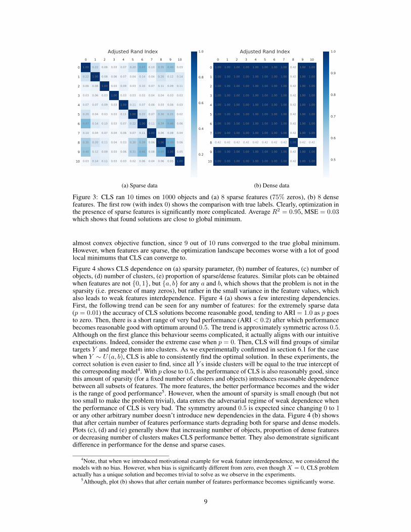
Figure 3 shows results of CLS evaluation when data consists of n = 1000 objects, 8 features whichare either all sparse with p = 0.25 (a) or all dense (b). Clearly, when features are dense, CLS has
8
0 1 2 3 4 5 6 7 8 9 10
0
1
2
3
4
5
6
7
8
9
10
1.00
0.22
0.06
0.03
0.07
0.20
0.47
0.10
0.35
0.40
0.03
0.22
1.00
0.08
0.06
0.07
0.04
0.14
0.04
0.20
0.12
0.14
0.06
0.08
1.00
0.03
0.09
0.03
0.10
0.07
0.11
0.09
0.11
0.03
0.06
0.03
1.00
0.03
0.03
0.03
0.04
0.04
0.03
0.03
0.07
0.07
0.09
0.03
1.00
0.11
0.07
0.06
0.03
0.06
0.03
0.20
0.04
0.03
0.03
0.11
1.00
0.22
0.07
0.30
0.31
0.02
0.47
0.14
0.10
0.03
0.07
0.22
1.00
0.11
0.39
0.46
0.06
0.10
0.04
0.07
0.04
0.06
0.07
0.11
1.00
0.06
0.08
0.04
0.35
0.20
0.11
0.04
0.03
0.30
0.39
0.06
1.00
0.49
0.06
0.40
0.12
0.09
0.03
0.06
0.31
0.46
0.08
0.49
1.00
0.05
0.03
0.14
0.11
0.03
0.03
0.02
0.06
0.04
0.06
0.05
1.00
Adjusted Rand Index
0.2
0.4
0.6
0.8
1.0
(a) Sparse data
0 1 2 3 4 5 6 7 8 9 10
0
1
2
3
4
5
6
7
8
9
10
1.00
1.00
1.00
1.00
1.00
1.00
1.00
1.00
0.42
1.00
1.00
1.00
1.00
1.00
1.00
1.00
1.00
1.00
1.00
0.42
1.00
1.00
1.00
1.00
1.00
1.00
1.00
1.00
1.00
1.00
0.42
1.00
1.00
1.00
1.00
1.00
1.00
1.00
1.00
1.00
1.00
0.42
1.00
1.00
1.00
1.00
1.00
1.00
1.00
1.00
1.00
1.00
0.42
1.00
1.00
1.00
1.00
1.00
1.00
1.00
1.00
1.00
1.00
0.42
1.00
1.00
1.00
1.00
1.00
1.00
1.00
1.00
1.00
1.00
0.42
1.00
1.00
1.00
1.00
1.00
1.00
1.00
1.00
1.00
1.00
0.42
1.00
1.00
0.42
0.42
0.42
0.42
0.42
0.42
0.42
0.42
1.00
0.42
0.42
1.00
1.00
1.00
1.00
1.00
1.00
1.00
1.00
0.42
1.00
1.00
1.00
1.00
1.00
1.00
1.00
1.00
1.00
1.00
0.42
1.00
1.00
Adjusted Rand Index
0.5
0.6
0.7
0.8
0.9
1.0
(b) Dense data
Figure 3: CLS ran 10 times on 1000 objects and (a) 8 sparse features (75% zeros), (b) 8 densefeatures. The first row (with index 0) shows the comparison with true labels. Clearly, optimization inthe presence of sparse features is significantly more complicated. Average R2 = 0.95, MSE = 0.03which shows that found solutions are close to global minimum.
almost convex objective function, since 9 out of 10 runs converged to the true global minimum.However, when features are sparse, the optimization landscape becomes worse with a lot of goodlocal minimums that CLS can converge to.
Figure 4 shows CLS dependence on (a) sparsity parameter, (b) number of features, (c) number ofobjects, (d) number of clusters, (e) proportion of sparse/dense features. Similar plots can be obtainedwhen features are not {0, 1}, but {a, b} for any a and b, which shows that the problem is not in thesparsity (i.e. presence of many zeros), but rather in the small variance in the feature values, whichalso leads to weak features interdependence. Figure 4 (a) shows a few interesting dependencies.First, the following trend can be seen for any number of features: for the extremely sparse data(p = 0.01) the accuracy of CLS solutions become reasonable good, tending to ARI = 1.0 as p goesto zero. Then, there is a short range of very bad performance (ARI < 0.2) after which performancebecomes reasonable good with optimum around 0.5. The trend is approximately symmetric across 0.5.Although on the first glance this behaviour seems complicated, it actually aligns with our intuitiveexpectations. Indeed, consider the extreme case when p = 0. Then, CLS will find groups of similartargets Y and merge them into clusters. As we experimentally confirmed in section 6.1 for the casewhen Y ∼ U(a, b), CLS is able to consistently find the optimal solution. In these experiments, thecorrect solution is even easier to find, since all Y s inside clusters will be equal to the true intercept ofthe corresponding model4. With p close to 0.5, the performance of CLS is also reasonably good, sincethis amount of sparsity (for a fixed number of clusters and objects) introduces reasonable dependencebetween all subsets of features. The more features, the better performance becomes and the wideris the range of good performance5. However, when the amount of sparsity is small enough (but nottoo small to make the problem trivial), data enters the adversarial regime of weak dependence whenthe performance of CLS is very bad. The symmetry around 0.5 is expected since changing 0 to 1or any other arbitrary number doesn’t introduce new dependencies in the data. Figure 4 (b) showsthat after certain number of features performance starts degrading both for sparse and dense models.Plots (c), (d) and (e) generally show that increasing number of objects, proportion of dense featuresor decreasing number of clusters makes CLS performance better. They also demonstrate significantdifference in performance for the dense and sparse cases.
4Note, that when we introduced motivational example for weak feature interdependence, we considered themodels with no bias. However, when bias is significantly different from zero, even though X = 0, CLS problemactually has a unique solution and becomes trivial to solve as we observe in the experiments.
5Although, plot (b) shows that after certain number of features performance becomes significantly worse.
9

0.0 0.2 0.4 0.6 0.8 1.0Sparsity parameter p
0.00
0.25
0.50
0.75
1.00
Aver
age
ARI
Mutual agreement
8 features16 features32 features
0.0 0.2 0.4 0.6 0.8 1.0Sparsity parameter p
0.00
0.25
0.50
0.75
1.00
Aver
age
ARI
Agreement with true labels
8 features16 features32 features
(a) 10000 objects, 4 clusters
0 50 100 150 200 250 300Number of features
0.0
0.5
1.0
Aver
age
ARI
Mutual agreementSparse features, p=0.25Sparse features, p=0.1Dense features
0 50 100 150 200 250 300Number of features
0.0
0.5
1.0
Aver
age
ARI
Agreement with true labelsSparse features, p=0.25Sparse features, p=0.1Dense features
(b) 10000 objects, 4 clusters
0 10000 20000 30000 40000 50000Number of objects
0.0
0.5
1.0
Aver
age
ARI
Mutual agreement
Sparse features, p=0.25Sparse features, p=0.1Dense features
0 10000 20000 30000 40000 50000Number of objects
0.0
0.5
1.0
Aver
age
ARI
Agreement with true labels
Sparse features, p=0.25Sparse features, p=0.1Dense features
(c) 16 features, 4 clusters
2 3 4 5 6 7 8 9 10Number of clusters
0.0
0.5
1.0
Aver
age
ARI
Mutual agreementSparse features, p=0.25Sparse features, p=0.1Dense features
2 3 4 5 6 7 8 9 10Number of clusters
0.5
1.0
Aver
age
ARI
Agreement with true labelsSparse features, p=0.25Sparse features, p=1Dense features
(d) 10000 objects, 16 features
0 2 4 6 8 10 12 14Number of dense features
0.00
0.25
0.50
0.75
1.00
Aver
age
ARI
Mutual agreement
p=0.25p=0.1
0 2 4 6 8 10 12 14Number of dense features
0.00
0.25
0.50
0.75
1.00
Aver
age
ARI
Agreement with true labels
p=0.25p=0.1
(e) 10000 objects, 4 clusters, 16 features
Figure 4: These plots demonstrate how different parameters affect the quality of CLS solutions.
Overall, the following conclusions were obtained:
• CLS clustering cannot be directly applied in the presence of features with weak interdepen-dence (which is the case when features are sparse), since optimization landscape becomeshighly non-convex with many good local minimums. When data has subsets of featureswith zero feature interdependence, the problem becomes ill-defined, since there are multipleoptimal solutions.
• Increasing proportion of dense/sparse features generally improves convergence.
• Increasing number of objectsnumber of features ratio generally improves convergence.
10

• Increasing true number of clusters makes problem harder (performance degrades significantlymore for the sparse case).
• Moving sparsity parameter closer to 0.5 generally improves convergence.
The main conclusion from these experiments is that in the presence of sparse features, even if thereexists a unique global optimum, it is unlikely to be found. And in some cases there are multipleglobal optimums and thus, finding actual clusters and coefficient that generated the data is impossible.Therefore, if interpretation of the clusters is the goal, it is necessary to redefine problem that CLSis solving in order to have a unique solution. One way to do so is to introduce, so-called, clusterseeds: objects that are restricted to be in a certain cluster and in some sense define a prior solutionto the problem. This prior is then refined when CLS recomputes clusters linear models and assignsnew points. It is also possible to control how much influence seeds should bring to the cluster modelby weighting seed objects (which is equivalent to implicitly adding the same seed objects to clustermultiple times). To make the contribution of seed and non-seed objects equal, seed weights could beset to
√N(i)
ns/N(i)s , where N (i)
ns , N(i)s are the number of seed and non-seed objects for cluster i. Of
course, if the seed objects are independent and the number of seeds equals the number of features,CLS problem will have a unique solution, since seeds would fully define corresponding linear models.When seed objects are representative of the true clusters, one could hope that having even smallnumber of seeds will provide enough information for CLS to converge to meaningful solutions. Incase when data was not actually generated from a mixture of linear models, seeds can still be usefulto define a clusters of interest. For example, if it is known that some objects behave differently fromthe others, placing them as cluster seeds will help to find more objects with similar characteristics.
7 Real-data experiments
7.1 Data analysis
Since the analysis of sparse data is complicated and requires careful tuning, we restrict our attentionto the dense corpus of hospital features. In this section we describe the application of CLS clusteringto a hospital-level data with a focus on finding meaningful clusters that can potentially be used as peergroups. We show that CLS clustering can provide additional insights into the found peer groups andcan be used to improve and refine final clusters with the correlation information. We start by applyingk-means with 4 clusters to the hospital-level data which is a traditional approach of obtaining hospitalpeer groups. K-means was initialized using k-means++ algorithm [2] and best out of 100 iterationswas chosen. We ignore the features corresponding to length of stay, since the goal is to obtain clustersbased on their operational characteristics. The length of stay information will be used later to refinethe analysis by applying CLS clustering. In order to visualize the results we use t-SNE technique [19]with 2 components. The found 4 clusters are depicted on Figure 5 (a).
In order to easier interpret the clustering results we use the following trick; for each cluster we train 2models: SVM with L1 regularization [30] and Random Forest [4] in order to classify points fromone cluster vs all the rest. We tune the regularization parameter of SVM to have only few non-zerofeatures and we also look at top-5 features according to feature importance produced by randomforest. The features found using this technique can be used to understand what separates one clusterfrom all the rest and thus gain an intuition into why the hospitals were assigned to that cluster. Thetop-3 features for each cluster are:
1. 991 hospitals: “type newborn”, “MDC 6” (digestive system), “MDC 5” (circulatory system)2. 416 hospitals: “type newborn”, “MDC 15” (newborns and neonates (perinatal period)),
“MDC 14” (pregnancy, childbirth)3. 169 hospitals: “MDC 20” (alcohol/drug use or induced mental disorders), “age”,
“MDC 19” (mental diseases and disorders)4. 586 hospitals: “age”, “MDC 23” (factors influencing health status), “type emergency’
Visually examining distributions of these features across the clusters we can further refine theunderstanding of obtained results. Cluster 2 seems to consists of hospitals specialized on pregnancyand childbirth. It has significantly higher average number of claims with type newborn, pregnancyand childbirth cases than all other clusters. Cluster 3 has a very high proportion of alcohol/drugillnesses as well as mental diseases comparing to other clusters. Cluster 4 has an average patient ageclose to 80 and seems to specialize on senior patients with a relatively small proportion of emergency
11

40 20 0 20 40 60t-SNE dim 1
40
20
0
20
40
t-SNE
dim
2
(a) k-means
40 20 0 20 40 60t-SNE dim 1
40
20
0
20
40
t-SNE
dim
2
(b) CLS + k-means
Figure 5: Comparison of (a) k-means clustering with (b) CLS clustering combined with k-means.Different clusters are depicted with different colors. Cluster centers are marked with white circles,indicating cluster indices.
claims. Cluster 1 contains large amount of hospitals with big proportion of digestive or circulatorysystems diagnosis, but a lot of hospitals from this cluster don’t have evident specialization.
Next, we apply CLS clustering on the same data to gain additional insights into the found clusters.CLS uses the same set of features as k-means for independent variables X and seeks clusters thatmaximize correlations with length of stay per MDC features Y . Running standard CLS doesn’t revealany clear structure in the found clusters with very low CLS objective values indicating that it mighthave overfitted the data producing non-intuitive solutions. Thus, we use the method introduced insection 6.2 of combining CLS with k-means objective on X features only. With βx = 0.01, βy = 0we obtain meaningful clusters that are depicted on Figure 5 (b). There are 2 interesting observations.Notice, that CLS doesn’t change cluster 4 significantly, while merging clusters 2 and 3 and splittingcluster 1 into two clusters. This illustrates that k-means clusters 2 and 3 have similar correlationpatters with length of stay and that cluster 1 is not correlation homogeneous. Examining CLScoefficients we can see that CLS clusters 1 and 4 (which k-means cluster 1 was split into) haveopposite correlations with, for example, “MDC 1 length” (nervous system), “MDC 4 length” and(respiratory system) “MDC 9 length” (skin, subcutaneous tissue and breast). However, we want toemphasize that since CLS coefficients are harder to interpret and might not be intuitively meaningful,it is important to verify any conclusions with a human expert in the field.
7.2 Prediction
In this section we demonstrate that CLS clustering can be used to improve length of stay predictionaccuracy for a claim-level data6. In this case Y consists of scalar values representing patient lengthof stay for a particular claim. It is not possible, however, to directly use linear regression modelsproduced by CLS clustering, since it is not clear how to assign labels to test data points for which Yis unknown. One way to do it is to build a separate classification model, predicting CLS labels fromfeatures X ∈ Rd. However, in many cases, d-dimensional planes produced by CLS clustering willoverlap and thus it might be impossible to predict the correct labels considering only features X andignoring the targets Y . A simple illustration of this problem is presented in Figure 6.
Manwani and Sastry [22] propose k-plane regression method that counteracts this problem bycombining CLS objective with k-means on features X only7. At test time authors propose to compute
6Note that since the goal of this section is not interpretation of the results, it doesn’t matter if CLS convergesto the “true” clusters generating the data, as long as it is helpful for prediction. Thus, the sparsity problemdescribed in section 6.3 does not matter as much in this case.
7We described this approach in section 6.2, however, aiming at different goal.
12

6 4 2 0 2 4 6X
6
4
2
0
2
4
6Y
Figure 6: This plot illustrates that it might be impossible to predict CLS labels from features Xonly. In this case there are 2 linear regressions that CLS would find, depicted with orange and blue.However, ignoring Y will make points from different clusters identical.
k-means centers of each cluster and assign new objects to clusters with closest centers. However,since the objective function has 2 potentially contradicting terms, it is not guaranteed that this criteriawill match points to the correct clusters even for the training data. Thus, even after combining CLSand k-means objectives, it might be beneficial to train additional classifier to predict CLS labels attest time. We call this method predictive CLS (CLSp) and compare its performance to the k-planeregression method of Manwani and Sastry [22]. Table 1 contains the results of the comparison. Tobetter understand the performance of both methods we used the following setup. First, the data isnormalized: each feature is divided by standard deviation with no mean subtraction8. Then, CLSclustering with varying number of clusters k and regularization coefficient βx was applied to thewhole dataset and cluster labels were recorder. We report the cross-validation9 performance of CLSmodels on the whole dataset in the second column of Table 1. These values show the performanceof prediction with CLS models if the true labels were known at test time10. Then, the dataset wassplit into train (75%) and test (25%) subsets. We predict test CLS labels using Random Forest forCLSp and closest cluster for k-plane. The accuracy of this prediction is reported in columns 3 and 4.After that we compute predictions for the length of stay values on a test subset using linear regressionmodels built with CLS for corresponding predicted clusters. These results are reported in columns 5,6. Notice that the performance of both CLSp and k-plane crucially depends on the labels predictionaccuracy. With k = 2, βx = 0, even though only 13% of the points are classified incorrectly, the R2
drops from potential 0.77 (when the true labels are known) to 0.21 for CLSp or −0.15 for k-planewhich is significantly worse than running a simple linear regression. The reason for that is becausedifferent CLS clusters have radically different regression coefficients and thus for any incorrectlyassigned label, the prediction might be arbitrary bad. Consider the example on Figure 6: if bluemodel is used for prediction of the orange dots, prediction becomes worse and worse farther from theorigin. In that case the best possible prediction model at test time would be a weighted combinationof the blue and orange models with equal weights. Even though this model will always predict zero,it is the best possible prediction when there is no prior knowledge about cluster labels for test objects.
We utilize this idea to improve the prediction results of CLSp. Instead of taking only the answer ofthe model predicted by random forest, we take a weighted average over models for all clusters withweights being equal to probabilities that a point belongs to certain cluster, which random forest cancompute. This approach is similar in spirit to performing a fuzzy CLR clustering (e.g. [9]) and couldpotentially be improved by incorporating fuzzy class memberships into the usual CLS procedure. Wereport the results of this weighting technique in columns 7 and 8 of Table 1. For k-plane weights areequal to the normalized distances to corresponding clusters.
8The reason for that is because the claim-level data is extremely sparse and thus it is possible to utilize fastsparse algorithms (e.g. LSQR [24] instead of the standard linear regression is used in all the models presentedbelow) for models training. Subtracting mean, however, would change the sparsity of the data and models willbecome much slower to train.
9For the description of this cross-validation process, see section 5.10Since we obtain cross-validation estimates of R2, the only overfitting present in this evaluation comes from
CLS itself: because we assume that we know the true labels.
13
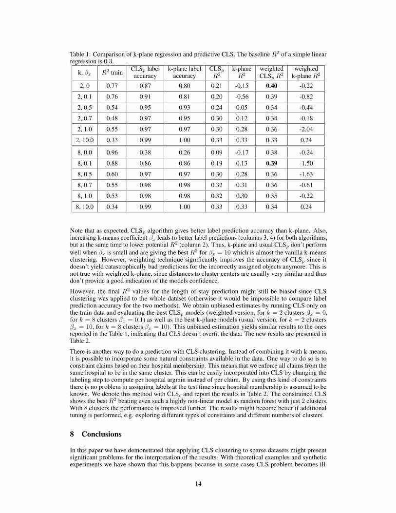
Table 1: Comparison of k-plane regression and predictive CLS. The baseline R2 of a simple linearregression is 0.3.
k, βx R2 train CLSp labelaccuracy
k-plane labelaccuracy
CLSp
R2k-planeR2
weightedCLSp R
2weighted
k-plane R2
2, 0 0.77 0.87 0.80 0.21 -0.15 0.40 -0.22
2, 0.1 0.76 0.91 0.81 0.20 -0.56 0.39 -0.82
2, 0.5 0.54 0.95 0.93 0.24 0.05 0.34 -0.44
2, 0.7 0.48 0.97 0.95 0.30 0.12 0.34 -0.18
2, 1.0 0.55 0.97 0.97 0.30 0.28 0.36 -2.04
2, 10.0 0.33 0.99 1.00 0.33 0.33 0.33 0.24
8, 0.0 0.96 0.38 0.26 0.09 -0.17 0.38 -0.24
8, 0.1 0.88 0.86 0.86 0.19 0.13 0.39 -1.50
8, 0.5 0.60 0.97 0.97 0.30 0.28 0.36 -1.63
8, 0.7 0.55 0.98 0.98 0.32 0.31 0.36 -0.61
8, 1.0 0.53 0.98 0.98 0.32 0.30 0.35 -0.22
8, 10.0 0.34 0.99 1.00 0.33 0.33 0.34 0.24
Note that as expected, CLSp algorithm gives better label prediction accuracy than k-plane. Also,increasing k-means coefficient βx leads to better label predictions (columns 3, 4) for both algorithms,but at the same time to lower potential R2 (column 2). Thus, k-plane and usual CLSp don’t performwell when βx is small and are giving the best R2 for βx = 10 which is almost the vanilla k-meansclustering. However, weighting technique significantly improves the accuracy of CLSp since itdoesn’t yield catastrophically bad predictions for the incorrectly assigned objects anymore. This isnot true with weighted k-plane, since distances to cluster centers are usually very similar and thusdon’t provide a good indication of the models confidence.
However, the final R2 values for the length of stay prediction might still be biased since CLSclustering was applied to the whole dataset (otherwise it would be impossible to compare labelprediction accuracy for the two methods). We obtain unbiased estimates by running CLS only onthe train data and evaluating the best CLSp models (weighted version, for k = 2 clusters βx = 0,for k = 8 clusters βx = 0.1) as well as the best k-plane models (usual version, for k = 2 clustersβx = 10, for k = 8 clusters βx = 10). This unbiased estimation yields similar results to the onesreported in the Table 1, indicating that CLS doesn’t overfit the data. The new results are presented inTable 2.
There is another way to do a prediction with CLS clustering. Instead of combining it with k-means,it is possible to incorporate some natural constraints available in the data. One way to do so is toconstraint claims based on their hospital membership. This means that we enforce all claims from thesame hospital to be in the same cluster. This can be easily incorporated into CLS by changing thelabeling step to compute per hospital argmin instead of per claim. By using this kind of constraintsthere is no problem in assigning labels at the test time since hospital membership is assumed to beknown. We denote this method with CLSc and report the results in Table 2. The constrained CLSshows the best R2 beating even such a highly non-linear model as random forest with just 2 clusters.With 8 clusters the performance is improved further. The results might become better if additionaltuning is performed, e.g. exploring different types of constraints and different numbers of clusters.
8 Conclusions
In this paper we have demonstrated that applying CLS clustering to sparse datasets might presentsignificant problems for the interpretation of the results. With theoretical examples and syntheticexperiments we have shown that this happens because in some cases CLS problem becomes ill-
14

Table 2: Comparison of different prediction models
MSE R2
Linear Regression 0.71 0.30
Random Forest 0.59 0.42
K-plane (2 clusters) 0.70 0.31
K-plane (8 clusters) 0.67 0.33
CLSp (2 clusters) 0.61 0.40
CLSp (8 clusters) 0.62 0.38
CLSc (2 clusters) 0.57 0.43
CLSc (8 clusters) 0.55 0.45
defined, meaning that there might be exponentially many potential solutions and thus, differentinterpretations. We also provide additional insights and interpretations of the problems of findingnon-intuitive solutions and overestimating the goodness of CLS fit that have been observed in theliterature before. Based on this preliminary analysis we show how CLS clustering can be potentiallyapplied to finding hospital peer-groups, which is an important problem for many health insuranceproviders. Finally, we propose new techniques to apply CLS for prediction and experimentally showthat on the problem of predicting patient length of stay they perform better than k-plane regression,linear regression and random forest.
References[1] J. A. Alexander, C. J. Evashwick, and T. Rundall. Hospitals and the provision of care to the
aged: a cluster analysis. Inquiry, pages 303–314, 1984.
[2] D. Arthur and S. Vassilvitskii. k-means++: The advantages of careful seeding. In Proceedingsof the eighteenth annual ACM-SIAM symposium on Discrete algorithms, pages 1027–1035.Society for Industrial and Applied Mathematics, 2007.
[3] A. M. Bagirov, A. Mahmood, and A. Barton. Prediction of monthly rainfall in victoria, australia:Clusterwise linear regression approach. Atmospheric Research, 188:20–29, 2017.
[4] L. Breiman. Random forests. Machine learning, 45(1):5–32, 2001.
[5] M. J. Brusco, J. D. Cradit, D. Steinley, and G. L. Fox. Cautionary remarks on the use ofclusterwise regression. Multivariate Behavioral Research, 43(1):29–49, 2008.
[6] M. J. Brusco, J. D. Cradit, and A. Tashchian. Multicriterion clusterwise regression for jointsegmentation settings: An application to customer value. Journal of Marketing Research,40(2):225–234, 2003.
[7] M. M. Byrne, C. N. Daw, H. A. Nelson, T. H. Urech, K. Pietz, and L. A. Petersen. Method todevelop health care peer groups for quality and financial comparisons across hospitals. Healthservices research, 44(2p1):577–592, 2009.
[8] R. A. da Silva and F. d. A. de Carvalho. On combining clusterwise linear regression and k-meanswith automatic weighting of the explanatory variables. In International Conference on ArtificialNeural Networks, pages 402–410. Springer, 2017.
[9] W. S. DeSarbo and W. L. Cron. A maximum likelihood methodology for clusterwise linearregression. Journal of classification, 5(2):249–282, 1988.
[10] X. Z. Fern, C. E. Brodley, and M. A. Friedl. Correlation clustering for learning mixtures ofcanonical correlation models. In Proceedings of the 2005 SIAM International Conference onData Mining, pages 439–448. SIAM, 2005.
15

[11] D. R. Hardoon, S. Szedmak, and J. Shawe-Taylor. Canonical correlation analysis: An overviewwith application to learning methods. Neural computation, 16(12):2639–2664, 2004.
[12] C. Hennig. Identifiability of Finite Linear Regression Mixtures. Universität Hamburg. Institutfür Mathematische Stochastik, 1996.
[13] H. Hotelling. Relations between two sets of variates. Biometrika, 28(3/4):321–377, 1936.
[14] L. Hubert and P. Arabie. Comparing partitions. Journal of classification, 2(1):193–218, 1985.
[15] C. Kang and S. Ghosal. Clusterwise regression using dirichlet mixtures. Advances in multivari-ate statistical methods, 4:305, 2009.
[16] H.-C. Kang, J.-S. Hong, and H.-J. Park. Development of peer-group-classification criteria forthe comparison of cost efficiency among general hospitals under the korean nhi program. Healthservices research, 47(4):1719–1738, 2012.
[17] T. D. Klastorin. An alternative method for hospital partition determination using hierarchicalcluster analysis. Operations Research, 30(6):1134–1147, 1982.
[18] E. Lei, K. Miller, and A. Dubrawski. Learning mixtures of multi-output regression models bycorrelation clustering for multi-view data. arXiv preprint arXiv:1709.05602, 2017.
[19] L. v. d. Maaten and G. Hinton. Visualizing data using t-sne. Journal of Machine LearningResearch, 9(Nov):2579–2605, 2008.
[20] L. MacNabb. Application of cluster analysis towards the development of health region peergroups. In Proceedings of the Survey Methods Section, pages 85–90. Citeseer, 2003.
[21] J. MacQueen et al. Some methods for classification and analysis of multivariate observations.In Proceedings of the fifth Berkeley symposium on mathematical statistics and probability,volume 1, pages 281–297. Oakland, CA, USA., 1967.
[22] N. Manwani and P. Sastry. K-plane regression. Information Sciences, 292:39–56, 2015.
[23] F. Murtagh and P. Contreras. Methods of hierarchical clustering. arXiv preprint arXiv:1105.0121,2011.
[24] C. C. Paige and M. A. Saunders. Lsqr: An algorithm for sparse linear equations and sparse leastsquares. ACM transactions on mathematical software, 8(1):43–71, 1982.
[25] A. Plaia. Constrained clusterwise linear regression. New Developments in Classification andData Analysis, pages 79–86, 2005.
[26] C. Reilly, C. Wang, and M. Rutherford. A rapid method for the comparison of cluster analyses.Statistica Sinica, pages 19–33, 2005.
[27] H. Späth. Algorithm 39 clusterwise linear regression. Computing, 22(4):367–373, 1979.
[28] D. Vicari and M. Vichi. Multivariate linear regression for heterogeneous data. Journal ofApplied Statistics, 40(6):1209–1230, 2013.
[29] N. X. Vinh, J. Epps, and J. Bailey. Information theoretic measures for clusterings comparison:Variants, properties, normalization and correction for chance. Journal of Machine LearningResearch, 11(Oct):2837–2854, 2010.
[30] J. Zhu, S. Rosset, R. Tibshirani, and T. J. Hastie. 1-norm support vector machines. In Advancesin neural information processing systems, pages 49–56, 2004.
[31] M. Zodet and J. Clark. Creation of hospital peer groups. Clinical performance and qualityhealth care, 4(1):51–57, 1996.
16