AlgorithmicaDOI 10.1007/s00453-013-9844-6

Capacitated Domination: Problem Complexityand Approximation Algorithms

Mong-Jen Kao · Han-Lin Chen · D.T. Lee

Received: 20 August 2012 / Accepted: 13 October 2013© Springer Science+Business Media New York 2013

Abstract We consider a local service-requirement assignment problem named ca-pacitated domination from an algorithmic point of view. In this problem, we aregiven a graph with three parameters defined on each vertex, which are the cost, thecapacity, and the demand, of a vertex, respectively. A vertex can be chosen multipletimes in order to generate sufficient capacity for the demands of the vertices in itsclosed neighborhood. The objective of this problem is to compute a demand assign-ment of minimum cost such that the demand of each vertex is fully-served by someof its closed neighbors without exceeding the amount of capacity they provide.

In this paper, we provide complexity results as well as several approximation al-gorithms to compose a comprehensive study for this problem. First, we provide log-arithmic approximations for general graphs which are asymptotically optimal. Fromthe perspective of parameterized complexity, we show that this problem is W [1]-hard

Extended abstracts of this work appeared in the 4th Frontiers of Algorithmics Workshop (FAW’10),Wuhan, China (received the best student paper award) [31] and the 22nd International Symposiumon Algorithms and Computation (ISAAC’11), Yokohama, Japan [32].

Part of this work was done when the author M.-J. Kao was with Karlsruhe Institute of Technology(KIT), Germany, as a visiting student.

M.-J. Kao (B) · D.T. LeeInstitute of Information Science, Academia Sinica, Taipei, Taiwane-mail: mong@iis.sinica.edu.tw

D.T. Leee-mail: dtlee@nchu.edu.tw

H.-L. ChenDepartment of Computer Science and Information Engineering, National Taiwan University, Taipei,Taiwan

Present address:D.T. LeeDepartment of Computer Science and Engineering, National Chung-Hsing University, Taichung,Taiwan

Algorithmica

with respect to treewidth and solution size. Moreover, we show that this problem isfixed-parameter tractable with respect to treewidth and the maximum capacity of thevertices. The latter result implies a pseudo-polynomial time approximation schemefor planar graphs under a standard framework.

In order to drop the pseudo-polynomial factor, we develop a constant-factor ap-proximation for planar graphs, based on a new perspective which we call generalladders on the hierarchical structure of outer-planar graphs. We believe that the ap-proach we use can be applicable to other capacitated covering problems.

Keywords Capacitated domination · Approximation algorithms · Dominating set ·Graph theory

1 Introduction

Resource management is one of the most important issues to be addressed in manyareas. One natural way to describe this scenario is to view resource management asa process of distributing resources to demanding targets. In some cases, there existlocality constraints between the supply and the demand, and it only makes sense toassign the resources from supplying source to demanding objects that lie in the neigh-borhood. Typical examples include communication in wireless ad-hoc networks, inwhich a peer can only be reached after entering the area it covers. This scenario isdepicted by the well-known and extensively studied dominating set problem. In thedominating set problem, we are given a graph G = (V ,E) and the objective is tocompute a vertex subset S of minimum cardinality such that for each vertex v ∈ V ,either v belongs to S or v has a neighbor that does.

In practice, the service-requirement relation between two vertices is often morecomplicated than a binary relation. To be more precise, the demand of each vertex ismore realistic when it is not simply assumed to be zero or one. The amount of supplyeach vertex can provide is often not unit or infinity. The cost of choosing a vertexinto the subset, i.e., the activation cost of vertices, is often not identical. Thereforeit is natural to take these quantities as part of the input instead of assuming them tobe simple constants. When we are allowed to activate the vertices multiple times inexchange of more supply, the scenario is said to be capacitated [22].

A series of study on capacitated covering problems was initiated by Guhaet al. [22], which addressed the vertex cover problem under the concept of capaci-tation, i.e., vertices are allowed to be chosen multiple times for more supply. Sev-eral follow-up papers have appeared since then, studying both this topic and relatedvariations [10, 19, 20]. These problems are also closely related to work on the ca-pacitated facility location problem, which has drawn a lot of attention since 1990s.See [9, 38, 40].

Motivated by the study on capacitated vertex covering and a more general localservice-requirement assignment scenario, Kao et al. [31–33] considered a generaliza-tion of the dominating set problem called capacitated domination. In this problem,the input graph G = (V ,E) is given along with three non-negative parameters de-fined on the set of vertices, which are referred to as the cost w : V → R

+ ∪ {0}, the

Algorithmica

capacity c : V → R+ ∪ {0}, and the demand d : V → R

+ ∪ {0}, respectively. Thedemand of a vertex stands for the amount of service it requires from its adjacent ver-tices, including the vertex itself. The capacity of a vertex represents the amount ofservice each multiplicity (copy) of that vertex can provide, and the cost of a vertex iswhat it requires to choose (activate) each multiplicity (copy) of that vertex.

In order to make the definition clear and to prevent confusion, we remark thatin this problem setting, a vertex is allowed to be chosen multiple times in order toprovide more service to its neighboring vertices, including itself.

By a demand assignment function f we mean a function which maps pairs of ver-tices to non-negative real numbers. Intuitively, f (u, v) denotes the amount of demandof u that is served by v. Throughout this paper, we also use the phrase “assigned to”alternatively with “served by” to indicate the demand assignment of a vertex for theease of presentation. We denote by NG(v) the set of neighbors of a vertex v ∈ V andby NG[v] = NG(v) ∪ {v} the set of closed neighbors of v.

Definition 1 (Feasible demand assignment function) A demand assignment functionf is said to be feasible if for each u ∈ V we have

∑

v∈NG[u]f (u, v) ≥ d(u).

That is, the demand assignment function is feasible if the demand of each vertex isfully-assigned to its closed neighbors.

For convenience, we say that a vertex u is dominated or served, following theclassical terminology, when the demand of u is fully assigned to its closed neighbors,i.e.,

∑v∈NG[u] f (u, v) ≥ d(u).

Given a demand assignment function f , the corresponding capacitated dominatingmulti-set D(f ) is defined as follows. For each vertex v ∈ V , the multiplicity of v inD(f ) is defined to be

xf (v) =⌈∑

u∈NG[v] f (u, v)

c(v)

⌉.

The cost of the assignment function f , denoted w(f ), is defined as

w(f ) =∑

v∈V

w(v) · xf (v).

Definition 2 (Capacitated domination problem) Given a graph G = (V ,E) with cost,capacity, and demand defined on each vertex, the capacitated domination problemasks for a feasible demand assignment function f such that w(f ) is minimized.

Depending on the way how the demand is assigned, there are different models toconsider. In the inseparable demand model we require that f (u, v) is either 0 or d(u),for each edge (u, v) ∈ E, while in the separable demand model we do not have suchconstraints. Intuitively, in the inseparable demand model we require that the demandof a vertex must be fully served merely by one of its closed neighbors.

Algorithmica

For the capacitated domination problem, Kao et al. [33], presented a (� + 1)-approximation for general graphs with separable demands, where � is the maxi-mum vertex degree of the graph. For trees with inseparable demands, they provided alinear-time algorithm that computes an exact solution. For trees with separable de-mands, they showed that this problem is NP-hard followed by presenting a fullypolynomial-time approximation scheme.

Dom et al. [13] considered a variation of this problem where the demand of eachvertex is unit and inseparable, and the number of multiplicities available at each ver-tex is limited by one. For this special case, they proved that this problem is W [1]-hardwhen parameterized by treewidth and solution size. Cygan et al. [11] considered thesame case and presented an exact algorithm with running time O(1.89n). The runningtime of this algorithm was further improved by Liedloff et al. [36] to O(1.8463n).

1.1 Related Work

The dominating set problem has been one of the most fundamental and well-knownproblems in both graph theory and combinatorial optimization for decades. As thisproblem is known to be NP-hard, approximation algorithms have been proposed inthe literature [3, 27, 29]. On the one hand, greedy algorithms are shown to achievea guaranteed ratio of lnn [29], where n is the number of vertices. The ratio is laterproven to be tight by Feige [15]. On the other hand, algorithms based on dual-fittingprovide a guaranteed ratio of � [27], where � is the maximum degree of the verticesin the graph. A polynomial-time approximation scheme for planar graphs was givenby Baker [3].

In terms of parameterized complexity, dominating set has its special place as well.In contrast to the vertex cover problem, which is fixed-parameter tractable (FPT) withrespect to solution size, i.e., can be solved in f (k) · nO(1) time where f (k) is a com-putable function of the solution size k and n is the number of vertices, dominating setis proven to be W [2]-complete, e.g., in [17, 37], in the sense that no fixed-parametertractable algorithm exists (with respect to solution size) unless FPT = W [2]. Al-though dominating set is a fundamentally hard problem in the parameterized W -hierarchy, it has been used as a benchmark problem for sub-exponential time param-eterized algorithms [1, 12, 18] and linear size kernels have been obtained for planargraphs [2, 8, 23, 24, 41], and more generally, for graphs that exclude a fixed graph H

as a minor [12].In addition, a considerable amount of work has been done in the literature, which

considers possible variations from purely theoretical aspects to practical applications.See [25, 39] for a detailed survey. In particular, variations of dominating set occur innumerous practical settings, ranging from strategic decisions, such as locating radarstations or emergency services, to computational biology and to voting systems. Forexample, Haynes et al. [26] considered the power domination problem in electricitynetworks [26, 35] while Wan et al. [43] considered the connected domination problemin wireless ad-hoc networks.

1.2 Our Contributions

The goal of this paper is to provide an overview on the problem complexity of thecapacitated domination problem with respect to different graph classes. In particu-

Algorithmica

lar, we present new approximation algorithms as well as complexity results for thisproblem. A table of summary on the results presented in this paper is also providedin Table 1.

First, we present logarithmic approximations with respect to both separable andinseparable demand models on general graphs. This is achieved by properly determin-ing a strategy that greedily selects a vertex with a specific property in each iteration.The idea we use for the inseparable demand model is relatively conceivable and pro-vides a hint towards separable demands for which a proper strategy is less obvious.This complements the previous approximation result, i.e., the (�+1)-approximationfor general graphs with separable demands [33], where � is the maximum vertexdegree of the graph, comparing to existing results for the classical dominating setproblem. Since the approximation threshold for the classical dominating set problemis known to be Ω(logn) [15], the results we present are also asymptotically optimalup to a constant factor.

Second, from the perspective of parameterized complexity, we prove that thisproblem is W [1]-hard when parameterized by treewidth and solution size, regard-less of demand assigning model. Then we present an exact FPT algorithm for bothdemand models with respect to treewidth and the maximum capacity of the vertices.

Although the embedding of the parameterized results into this paper may appear tobe rather loose, it plays an important role in the overview of our study. On one hand,the hardness result provides a justification to further exploration of approximationalgorithms for these graphs, as it is unlikely that we can solve this problem efficientlyeven when the treewidth is low. On the other hand, the algorithmic result we providein this section will further serve as a basis to our results for planar graphs that follow.

As a step towards getting polynomial-time approximations for planar graphs,we consider outerplanar graphs, i.e., planar graphs of low treewidth, and present a

Table 1 Summary of our results. In this table, n denotes the number of vertices

Inseparable demand Separable demand

General graphs (lnn)-Approximation, Theorem 1 (4 lnn + 2)-Approximation,Theorem 3

(2 lnn + 1)-Approximation for unitvertex cost, Theorem 4

W [1]-hard when parameterized by treewidth, Theorem 5

FPT w.r.t. treewidth and maximum vertex capacity

Graphs ofboundedtreewidth

Exact solution in timeO(k · 22k(logM+1)n),Theorem 6

Exact solution in timeO(2(2M+2N+1) logkn),Corollary 2

k: treewidth

M: the maximum capacity, N : the maximum demand

(1 + ε)-Approx. in pseudo-poly time, Theorem 9

Planar graphs Cannot be approximatedto a factor better than( 3

2 − ε), for any ε > 0,Theorem 10

80-Approximation inpolynomial time,Theorem 11

Algorithmica

constant-factor approximation for separable demands. To this end, we handle thestructure of outerplanar graphs using a new approach that enables us to tackle ver-tices of large degrees. This is crucial since in most of the techniques which trans-form pseudo-polynomial time algorithms into constant-factor approximations, theerror produced between neighboring vertices is accumulated at the vertices via theedges. For vertices of large degrees, the overall error would not be bounded.

To be more precise, we use a new perspective on the hierarchical structure of outer-planar graphs, which enables us to simply the underlying structure by analyzing theprimal linear program of this problem. To obtain an approximation for the reducedstructure, we further analyze the dual linear program. We believe that the approach weused can be applicable to other capacitated covering problems to help tackle verticesof large degrees as well.

Then, as an overview to the problem complexity on planar graphs, we presentpseudo-polynomial-time approximation schemes for both demand models andconstant-factor approximations for separable demands by generalizing the above al-gorithms under a standard framework due to Baker [3]. Although the former onefollows directly, the second one requires slight modifications and careful augmenta-tion of the algorithm proposed for outerplanar graphs. On the negative side, we provea lower bound of ( 3

2 − ε) for the approximation ratio of any algorithm for planargraphs with inseparable demands, for any ε > 0.

1.3 Organization of this Paper

The rest of this paper is organized as follows. In Sect. 2 we define the basic termi-nologies that will be used throughout this paper. In Sect. 3 we present our logarithmicapproximation algorithms for both inseparable and separable demand models on gen-eral graphs.

In Sect. 4 we present our parameterized results. In Sect. 5 we develop a constant-factor approximation algorithm for the separable demand model on outerplanargraphs. In Sect. 6 we apply and combine the results obtained in Sects. 4 and 5 tojointly compose a study for both demand models on planar graphs. Finally we con-clude in Sect. 7 with a brief overview and a discussion on future directions.

2 Preliminaries

We assume that all the graphs considered in this paper are simple, connected, andundirected. Let G = (V ,E) be a graph. We denote the number of vertices, |V |, by n.The set of neighbors of a vertex v ∈ V is denoted by NG(v) = {u : [u,v] ∈ E}. Theclosed neighborhood of v ∈ V is denoted by NG[v] = NG(v) ∪ {v}. We use “degreeof v” and “closed degree of v”, written degG(v) and degG[v], to denote the cardinal-ity of NG(v) and NG[v], respectively. The subscript G in NG[v] and degG[v] will beomitted when the considered graph is clear from the context.

Planar and Outerplanar Graphs A planar embedding of a graph G is a drawingof G in the plane such that the edges intersect only at their endpoints. A graph issaid to be planar if it has a planar embedding. An outer-planar graph is a graph which

Algorithmica

allows for a planar embedding such that all the vertices lie on a fixed circle, and all theedges are straight lines drawn inside the circle. For k ≥ 1, k-outerplanar graphs aredefined as follows. A graph is 1-outerplanar if and only if it is outer-planar. For k > 1,a graph is called k-outerplanar if it has a planar embedding such that the removal ofthe vertices on the unbounded face results in a (k − 1)-outerplanar graph.

Parameterized Complexity and Tree Decomposition Parameterized complexity is awell-developed framework for studying computationally hard problems [14, 17, 37].A problem is called fixed-parameter tractable (FPT) with respect to a parameter k ifit can be solved in time f (k) · nO(1), where f is a computable function dependingonly on k. Problems (along with its defining parameters) being W [t]-hard for anyt ≥ 1 are believed not to admit any FPT algorithms (with respect to the specifiedparameters). Now we define the notion of parameterized reduction.

Definition 3 (Parameterized reduction) Let A and B be two parameterized problems.We say that A reduces to B by a parameterized reduction if there exists an algorithmΦ that transforms (x, k) into (x′, g(k)) in time f (k) · |x|O(1), where f,g :N → N arearbitrary functions, such that (x, k) ∈ A if and only if (x′, g(k)) ∈ B .

Among the diverse choices of parameters, a common and widely-used one that isalso closely related to the structure of the input graph is the treewidth [6, 34], whichwe will define in the following. This parameter is particularly useful when dealingwith planar graphs. See also [3, 37]. We start with the concept of tree decomposition.

Definition 4 (Tree decomposition of a graph) A tree decomposition of a graph G =(V ,E) is a pair (X = {Xi : i ∈ I }, T = (I,F )) where each node i ∈ I is associatedwith a subset of vertices Xi ⊆ V , called the bag of i, such that the following holds.

1. Each vertex belongs to at least one bag:⋃

i∈I Xi = V .2. For each edge (u, v) ∈ E, there is a bag containing its end-points, u and v.3. For all vertices v ∈ V , the set of nodes containing v, which is {i ∈ I : v ∈ Xi},

induces a subtree of T .

The width of a tree decomposition is defined as maxi∈I |Xi | − 1. The treewidth ofa graph G is the minimum width over all possible tree decompositions of G.

3 Logarithmic Approximations for General Graphs

In this section, we present logarithmic approximation algorithms for capacitateddomination problems with respect to each of the two demand models. Specifically,we provide a (lnn)-approximation for the inseparable demand model, where n is thenumber of vertices. For the separable demand model, a (4 lnn + 2)-approximation ispresented. For the case of unit vertex costs,we give a (2 lnn + 1)-approximation.

This is achieved by properly determining a strategy that greedily selects a vertexwith a specific property in each iteration. The idea we use for the inseparable demandmodel is relatively conceivable and provides a hint towards separable demands, forwhich a proper strategy is less obvious.

Algorithmica

3.1 (lnn)-Approximation for the Inseparable Demand Model

Below we present our algorithm, denoted Π∗, for the inseparable demand model. LetG = (V ,E) be the input graph and U be the set of vertices which have not yet beenserved (dominated). Initially, we have U = V . For each vertex u ∈ V , let Nud [u] =U ∩ N [u] be the set of undominated vertices in the closed neighborhood of u.

In each iteration, Π∗ chooses a vertex of the greatest efficiency from V , wherethe efficiency of a vertex, say u, is defined by the largest ratio between the num-ber of vertices to be dominated by u and the total cost required by this assign-ment, among all possible demand assignments from Nud [u] to u. To be precise, letvu,1, vu,2, . . . , vu,|Nud [u]| denote the undominated neighbors Nud [u] of u, sorted innon-decreasing order of their demands. The efficiency of u is defined to be

δ(u) := max1≤i≤|Nud [u]|

i

w(u) · xu(i), where xu(i) =

⌈∑1≤j≤i d(vu,j )

c(u)

⌉

is the number of copies of u necessary to dominate vu,1, vu,2, . . . , vu,i . For consis-tency, we define δ(u) to be zero when Nud [u] is empty. Let u0 be the vertex ofmaximum efficiency, and δ−1(u0) denote the corresponding index such that the ra-tio i/(w(u0) · xu0(i)) is maximized. The algorithm removes the set of vertices to bedominated, vu0,1, vu0,2, . . . , vu0,δ

−1(u0), from U and assigns their demands to u0. This

process continues until U = ∅.

Theorem 1 Algorithm Π∗ computes a (lnn)-approximation for the capacitateddomination problem with inseparable demands in O(n3) time, where n is the numberof vertices.

Proof For the correctness of this algorithm, since it only removes vertices from Uwhen their demand is assigned, it always produces a feasible demand assignmentfunction. In the following we prove that this assignment function gives a (lnn)-approximation.

For each iteration, say, j , let OPTj denote the cost of the optimal demand assign-ment function for the remaining problem instance. Clearly, we have OPTj ≤ OPT ,where OPT is the cost of the optimal demand assignment function for the originalproblem instance. Let the cardinality of U at the beginning of iteration j be nj , andlet kj = nj − nj+1 be the number of vertices that are newly dominated in iteration j .

Denote by Sj the cost we spend in iteration j . Assume that Π∗ repeats for m itera-tions. Since we always choose the vertex with the maximum efficiency, the efficiencyof the chosen vertex is no less than the efficiency of each vertex chosen in OPTj , andtherefore no less than any weighted average of them, including nj/OPTj . In otherwords, we have

kj

Sj

≥ nj

OPTj

,

which implies that

Sj ≤ kj

nj

· OPTj , for all j with 1 ≤ j ≤ m.

Algorithmica

Taking the sum over all Sj and observing that nj+1 = nj − kj , we obtain

∑

1≤j≤m

Sj ≤∑

1≤j≤m

kj

nj

· OPTj ≤( ∑

1≤j≤n

1

j

)· OPT ≤ lnn · OPT,

where the second inequality follows from the fact that

kj

nj

≤ 1

nj

+ 1

nj − 1+ 1

nj − 2+ · · · + 1

nj − kj + 1=

∑

nj+1<i≤nj

1

i.

To see that the time complexity is O(n3), notice that it requires O(n) time to com-pute a most efficient move for each vertex, which leads to an O(n2) computation forthe most efficient choice in each iteration. The number of iterations is upper boundedby O(n) since at least one vertex is satisfied in each iteration.

We remark that, although it may appear that the time it requires to fetch the mostefficient move in each iteration can be further improved, the number of updates re-quired to maintain the supporting data structure could easily amount up to O(n),which makes this possibility unlikely to exist. �

3.2 (4 lnn + 2)-Approximation for the Separable Demand Model

We present an algorithm Π s that computes a (4 lnn+ 2)-approximation for the sepa-rable demand model. As the demand may be partially assigned during the algorithm,for each vertex u ∈ V , we denote by rd(u) the amount of demand of u that has not yetbeen served. For convenience we also refer to this quantity, rd(u), as residue demandof u, and to the fraction, rd(u)/d(u), as the remaining portion of u. Initially, rd(u) isset to be d(u), and will be updated accordingly when a fraction of the residue demandis assigned. The vertex u is said to be dominated when rd(u) = 0.

In each iteration, algorithm Π s performs two stages of greedy choices. First, itchooses the vertex of the most efficiency from V , where the efficiency is definedin a similar fashion as in the previous section with some modification due to theseparability of the demand.

For each vertex u ∈ V , let Nud [u] = {vu,1, vu,2, . . . , vu,|Nud [u]|} denote the setof undominated neighbors of u, sorted in non-descending order with respect totheir demands. Let ju, 0 ≤ ju ≤ |Nud [u]|, be the largest integer such that c(u) ≥∑ju

i=1 rd(vu,i). In other words, we choose the largest index ju such that the residuedemand of the first ju vertices in the sorted list could be served by one single copyof u. Let X(u) = ∑ju

i=1rd(vu,i )

d(vu,i )be the corresponding sum of remaining portion. In

addition, to effectively use the remaining capacity provided by this single copy of u,we let

Y(u) = c(u) − ∑ju

i=1 rd(vu,i)

d(vu,ju+1)

if ju < |Nud [u]| and Y(u) = 0 otherwise. Since we select the vertices in the sortedorder of their demands, one can easily verify that this always results in the maximum

Algorithmica

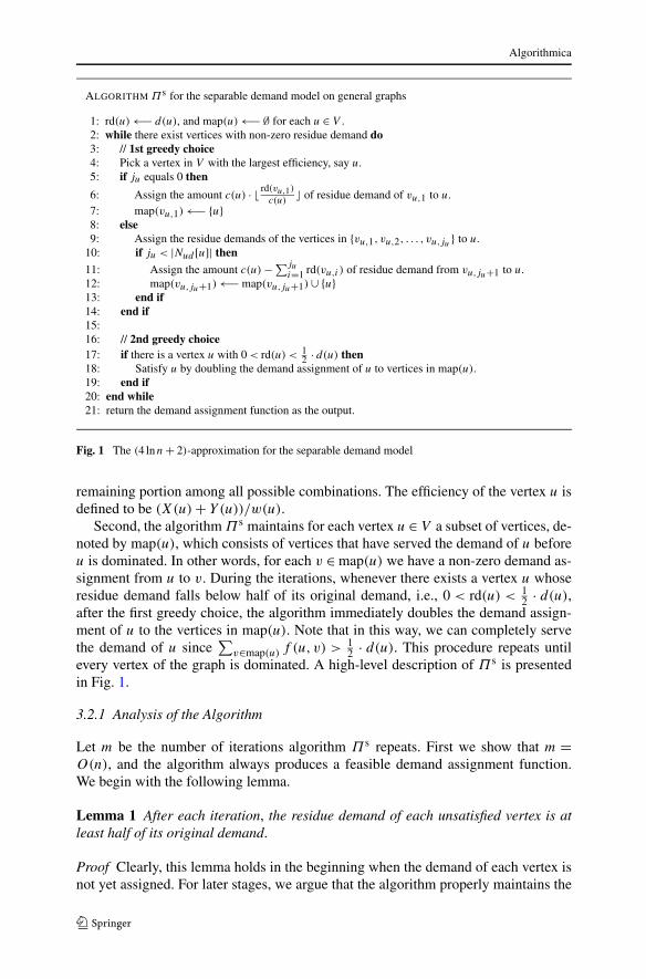
ALGORITHM Πs for the separable demand model on general graphs

1: rd(u) ←− d(u), and map(u) ←− ∅ for each u ∈ V .2: while there exist vertices with non-zero residue demand do3: // 1st greedy choice4: Pick a vertex in V with the largest efficiency, say u.5: if ju equals 0 then

6: Assign the amount c(u) · rd(vu,1)

c(u)� of residue demand of vu,1 to u.

7: map(vu,1) ←− {u}8: else9: Assign the residue demands of the vertices in {vu,1, vu,2, . . . , vu,ju } to u.

10: if ju < |Nud [u]| then

11: Assign the amount c(u) − ∑jui=1 rd(vu,i ) of residue demand from vu,ju+1 to u.

12: map(vu,ju+1) ←− map(vu,ju+1) ∪ {u}13: end if14: end if15:16: // 2nd greedy choice17: if there is a vertex u with 0 < rd(u) < 1

2 · d(u) then18: Satisfy u by doubling the demand assignment of u to vertices in map(u).19: end if20: end while21: return the demand assignment function as the output.

Fig. 1 The (4 lnn + 2)-approximation for the separable demand model

remaining portion among all possible combinations. The efficiency of the vertex u isdefined to be (X(u) + Y(u))/w(u).

Second, the algorithm Π s maintains for each vertex u ∈ V a subset of vertices, de-noted by map(u), which consists of vertices that have served the demand of u beforeu is dominated. In other words, for each v ∈ map(u) we have a non-zero demand as-signment from u to v. During the iterations, whenever there exists a vertex u whoseresidue demand falls below half of its original demand, i.e., 0 < rd(u) < 1

2 · d(u),after the first greedy choice, the algorithm immediately doubles the demand assign-ment of u to the vertices in map(u). Note that in this way, we can completely servethe demand of u since

∑v∈map(u) f (u, v) > 1

2 · d(u). This procedure repeats untilevery vertex of the graph is dominated. A high-level description of Π s is presentedin Fig. 1.

3.2.1 Analysis of the Algorithm

Let m be the number of iterations algorithm Π s repeats. First we show that m =O(n), and the algorithm always produces a feasible demand assignment function.We begin with the following lemma.

Lemma 1 After each iteration, the residue demand of each unsatisfied vertex is atleast half of its original demand.

Proof Clearly, this lemma holds in the beginning when the demand of each vertex isnot yet assigned. For later stages, we argue that the algorithm properly maintains the

Algorithmica

set map(u) for each vertex u ∈ V such that in our second greedy choice, wheneverthere exists a vertex u with 0 < rd(u) < 1

2 · d(u), it is always sufficient to double thedemand assignment f (u, v) for each v ∈ map(u). If map(u) is only modified underthe condition 0 < jv < |Nud [v]| (line 12 in Fig. 1), then map(u) contains exactly theset of vertices that have partially served u. Therefore we have

∑v∈map(u) f (u, v) >

12d(u), and it is sufficient to double the demand assignment in this case. If map(u)

is reassigned under the condition jv = 0 at some stage, then we have c(v) < rd(u) ≤d(u). Since we assign the amount c(v) · rd(u)/c(v)� of residue demand of u to v,this leaves at most half amount of the original residue demand of u, which is alsono larger than c(v). Therefore u will be immediately dominated by doubling thisassignment in the same iteration. �

For each iteration j , 1 ≤ j ≤ m, let uj be the chosen vertex of the maximumefficiency and nj = ∑

u∈V rd(u)/d(u) be the sum of the remaining portion over allvertices at the beginning of that iteration. For the ease of presentation, nj is defined tobe zero for j > m. We have the following lemma regarding the changes of nj over j .

Lemma 2 For each j with 1 ≤ j ≤ m, we have nj − nj+1 ≥ 12 .

Proof For iteration j , 1 ≤ j ≤ m, let uj be the chosen vertex of the maximum effi-ciency. Observe that vuj ,1 will be satisfied after this iteration. By Lemma 1, we have

rd(vuj ,1)/d(vuj ,1) ≥ 12 . Therefore the remaining portion covered in each iteration is

at least half. �

Since the algorithm repeats until all vertices are satisfied, by Lemma 2, we knowthat m ≤ 2n, and the resulting demand assignment is feasible.

In the following we show that the demand assignment function is indeed a(4 lnn + 2) approximation. Let the cost incurred by the first greedy choice be S1and the cost by the second choice be S2. To see that the solution achieves the desiredapproximation guarantee, notice that S2 is bounded from above by S1, for what wedo in the second choice is merely to satisfy the residue demand of a vertex, if thereexists one, by doubling its previous demand assignment.

It remains to bound the cost S1. For each iteration j , 1 ≤ j ≤ m, let uj be thechosen vertex of the maximum efficiency and OPTj be the cost of the correspondingoptimal demand assignment function of this remaining problem instance. Denote byS1,j the cost incurred by the first greedy choice in iteration j . We have the followingtwo lemmas.

Lemma 3 For each j , 1 ≤ j ≤ m, we have

S1,j ≤ nj − nj+1

nj

· OPTj ,

where nj − nj+1 is the remaining portion covered by uj in iteration j .

Proof The optimality of our choice in each iteration is obvious since we consider theelements of Nud [u] in sorted order according to their demands. Note that only in the

Algorithmica

case c(u) < rd(vu,1), the algorithm could possibly take more than one copy. In thiscase the efficiency of our choice remains unchanged since the cost and the remainingportion covered by u grows by the same factor. Therefore the efficiency of our choice,(nj − nj+1)/S1,j , is always no less than the efficiency of each chosen vertex in theoptimal solution, and therefore no less than any of their weighted averages, includingnj/OPTj . Therefore this lemma follows. �

Lemma 4m−1∑

j=1

�nj − nj+1� nj � ≤ 2 lnn

Proof Note that we have nj ≥ 1 for all j < m, since, whenever nj < 1, the remainingportion will be covered in the same iteration according to Lemmas 1 and 2. We willargue that each item of this series together constitutes at most two harmonic series.

By expanding the summand we have

�nj − nj+1� nj� ≤ 1

nj� + 1

nj� − 1+ · · · + 1

nj� − �nj − nj+1� + 1(1)

Since

nj+1� = ⌊nj − (nj − nj+1)

⌋

≤ nj� − nj − nj+1� ≤ nj� − �nj − nj+1� + 1,

possible repetitions of the expanded items only occur at the first item and the last itemof (1) if we expand each summand from the summation. By Lemma 2, the decreasebetween nj and nj+1 is at least half. Therefore, each repeated item, 1/( nj �− �nj −nj+1� + 1), will never occur more than twice in the expansion, and we can concludethat

∑m−1j=1 �nj − nj+1�/ nj� ≤ 2 lnn. �

We conclude our result in the following theorem.

Theorem 2 Algorithm Π s computes a (4 lnn+2)-approximation for the capacitateddomination problem with separable demands in polynomial-time.

Proof By Lemma 3, we have

m∑

j=1

S1,j ≤m−1∑

j=1

nj − nj+1

nj

· OPTj + nm

nm

· OPTm

≤(

m−1∑

j=1

�nj − nj+1� nj� + 1

)· OPT,

where the second inequality follows from the fact that r� ≤ r ≤ �r� for any realnumber r and OPTj ≤ OPT for each 1 ≤ j ≤ m. By Lemma 4, the cost of the demand

Algorithmica

assignment function returned by algorithm Π s is bounded by

S1 + S2 ≤ 2 · S1 = 2 ·m∑

j=1

S1,j ≤ 2 · (2 lnn + 1) · OPT.

This proves the theorem. �

3.2.2 Regarding the Technical Implementation Details

A naïve implementation of this algorithm leads to a running time cubic in the numberof vertices. However, by exploiting the property we assumed during the iterations thatthe undominated neighbors of each vertex are sorted in non-descending order accord-ing their demands, we can improve the running time of the algorithm to O(n2 logn),which is also the time required to build the sorted list of the closed neighborhood foreach vertex.

Theorem 3 Algorithm Π s computes a (4 lnn + 2)-approximation for the capaci-tated domination problem with separable demands in O(n2 logn) time, where n isthe number of vertices.

Proof Below we describe the implementation detail of this improvement. The ideais to maintain the efficiency of each vertex in a binary max-heap. In each iteration,we extract the vertex of the greatest efficiency from the heap, perform the demandassignments suggested by the most efficient move, and update the efficiencies of thevertices affected by each demand assignment.

To this end, for each vertex, we maintain a pointer to the vertex in its closed neigh-borhood that corresponds to the last item in the most efficient move. The pointerstored for each vertex will iterate over its closed neighborhood in sorted order atmost once upon updates. Whenever the residue demand of a vertex, say u, gets as-signed, we update the efficiencies as well as the most efficient moves of its closedneighborhood accordingly. To be more precise, for each v ∈ N [u], depending on therelative position of u and the vertex to which the pointer of v points in N [v], wehave two cases. If u lies after the pointer, then no updates are required. Otherwise weiterate the pointer of v according to our predefined notion of efficiency.

Since at least one vertex will be dominated and at most one vertex will be partiallyassigned in each iteration, the number of partial assignment will be no more than n.For each demand assignment, the number of updates required is bounded by the car-dinality of the closed neighborhood, which is O(n). Therefore, the total number ofupdates is O(n2). Since the pointer we maintained for each vertex is iterated overits closed neighborhood at most once, the time required for all the updates is alsobounded by O(n2).

For the running time of the whole algorithm, it takes O(n2 logn) time to buildthe sorted list for each vertex. In each iteration, it takes O(logn) time to extract andto maintain the heap property, provided that the efficiency of each vertex is updated.The total time required to perform the update is O(n2) from the above discussion.Therefore the overall time complexity is O(n2 logn). �

Algorithmica

3.3 (2 lnn + 1)-Approximation for Separable Demand Model with Unit Vertex Cost

We show that, when the demand is separable and each vertex has uniform cost, wecan compute a (2 lnn + 1)-approximation in polynomial time. To this end, we firstmake a reduction on the problem instance by spending a cost of at most OPT suchthat it takes at most one copy to serve each remaining undominated vertex. Thenwe show that a (2 lnn)-approximation can be computed for this reduced probleminstance, following a similar approach proposed in the last section.

For each u ∈ V , let gu ∈ N [u] be the vertex with the maximum capacity. First, foreach u ∈ V , we assign c(gu) · d(u)

c(gu)� of the demand of u to gu. Let S be the total cost

incurred by this assignment. We have the following Lemma 5.

Lemma 5 We have S ≤ OPT , where S is the total cost incurred by assigning c(gu) · d(u)

c(gu)� demand of the vertex u to gu, for all u ∈ V , and OPT is the cost of the optimal

demand assignment function.

Proof Notice that, when fractional multiplicities are allowed, an optimal demandassignment O∗ can be obtained by assigning the demand d(u) of u to gu, for eachvertex u. Let

w∗(O∗) =∑

u∈V

w(u) ·∑

v∈N [u] O∗(v,u)

c(u)

be the total cost required by O∗. Since S ≤ w∗(O∗) and w∗(O∗) ≤ OPT , the lemmafollows. �

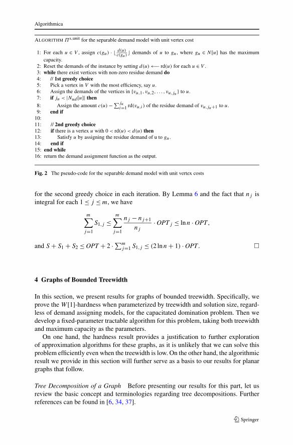
In the following, we will assume that d(u) ≤ c(gu), for each u ∈ V . The algorithmprovided in Sect. 3.2 is slightly modified. In particular, for the second greedy choice,whenever rd(u) < d(u) for some vertex u ∈ V , we immediately assign the residue de-mand of u to gu. Let Π s,unit denote this modified algorithm. A high-level descriptionof this algorithm is also given in Fig. 2. Recall that nj is the total remaining portionsof the vertices at the beginning of iteration j . We have the following lemma, whichis an updated version of Lemma 2.

Lemma 6 We have nj − nj+1 ≥ 1 for each 1 ≤ j ≤ m.

Proof Observe that in each iteration, at least one vertex is dominated and the residuedemand of each vertex is either 0 or equal to its original demand. �

We conclude this result in the following theorem.

Theorem 4 Algorithm Π s,unit computes a (2 lnn + 1)-approximation in timeO(n2 logn) for the capacitated domination problem with separable demand anduniform costs, where n is the number of vertices.

Proof We adopt the notation from the previous section. Clearly, S2 is bounded aboveby S1, as we always take one copy for the first greedy choice and at most one copy

Algorithmica

ALGORITHM Πs,unit for the separable demand model with unit vertex cost

1: For each u ∈ V , assign c(gu) · d(u)c(gu)

� demands of u to gu, where gu ∈ N [u] has the maximumcapacity.

2: Reset the demands of the instance by setting d(u) ←− rd(u) for each u ∈ V .3: while there exist vertices with non-zero residue demand do4: // 1st greedy choice5: Pick a vertex in V with the most efficiency, say u.6: Assign the demands of the vertices in {vu,1, vu,2, . . . , vu,ju } to u.7: if ju < |Nud [u]| then

8: Assign the amount c(u) − ∑jui=1 rd(vu,i ) of the residue demand of vu,ju+1 to u.

9: end if10:11: // 2nd greedy choice12: if there is a vertex u with 0 < rd(u) < d(u) then13: Satisfy u by assigning the residue demand of u to gu.14: end if15: end while16: return the demand assignment function as the output.

Fig. 2 The pseudo-code for the separable demand model with unit vertex costs

for the second greedy choice in each iteration. By Lemma 6 and the fact that nj isintegral for each 1 ≤ j ≤ m, we have

m∑

j=1

S1,j ≤m∑

j=1

nj − nj+1

nj

· OPTj ≤ lnn · OPT,

and S + S1 + S2 ≤ OPT + 2 · ∑mj=1 S1,j ≤ (2 lnn + 1) · OPT . �

4 Graphs of Bounded Treewidth

In this section, we present results for graphs of bounded treewidth. Specifically, weprove the W [1]-hardness when parameterized by treewidth and solution size, regard-less of demand assigning models, for the capacitated domination problem. Then wedevelop a fixed-parameter tractable algorithm for this problem, taking both treewidthand maximum capacity as the parameters.

On one hand, the hardness result provides a justification to further explorationof approximation algorithms for these graphs, as it is unlikely that we can solve thisproblem efficiently even when the treewidth is low. On the other hand, the algorithmicresult we provide in this section will further serve as a basis to our results for planargraphs that follow.

Tree Decomposition of a Graph Before presenting our results for this part, let usreview the basic concept and terminologies regarding tree decompositions. Furtherreferences can be found in [6, 34, 37].

Algorithmica

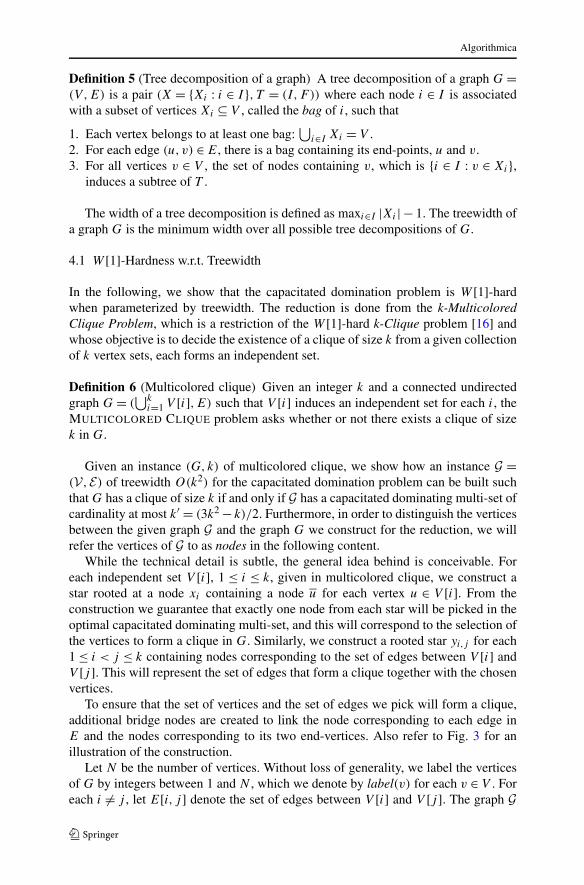
Definition 5 (Tree decomposition of a graph) A tree decomposition of a graph G =(V ,E) is a pair (X = {Xi : i ∈ I }, T = (I,F )) where each node i ∈ I is associatedwith a subset of vertices Xi ⊆ V , called the bag of i, such that

1. Each vertex belongs to at least one bag:⋃

i∈I Xi = V .2. For each edge (u, v) ∈ E, there is a bag containing its end-points, u and v.3. For all vertices v ∈ V , the set of nodes containing v, which is {i ∈ I : v ∈ Xi},

induces a subtree of T .

The width of a tree decomposition is defined as maxi∈I |Xi | − 1. The treewidth ofa graph G is the minimum width over all possible tree decompositions of G.

4.1 W [1]-Hardness w.r.t. Treewidth

In the following, we show that the capacitated domination problem is W [1]-hardwhen parameterized by treewidth. The reduction is done from the k-MulticoloredClique Problem, which is a restriction of the W [1]-hard k-Clique problem [16] andwhose objective is to decide the existence of a clique of size k from a given collectionof k vertex sets, each forms an independent set.

Definition 6 (Multicolored clique) Given an integer k and a connected undirectedgraph G = (

⋃ki=1 V [i],E) such that V [i] induces an independent set for each i, the

MULTICOLORED CLIQUE problem asks whether or not there exists a clique of sizek in G.

Given an instance (G, k) of multicolored clique, we show how an instance G =(V,E) of treewidth O(k2) for the capacitated domination problem can be built suchthat G has a clique of size k if and only if G has a capacitated dominating multi-set ofcardinality at most k′ = (3k2 − k)/2. Furthermore, in order to distinguish the verticesbetween the given graph G and the graph G we construct for the reduction, we willrefer the vertices of G to as nodes in the following content.

While the technical detail is subtle, the general idea behind is conceivable. Foreach independent set V [i], 1 ≤ i ≤ k, given in multicolored clique, we construct astar rooted at a node xi containing a node u for each vertex u ∈ V [i]. From theconstruction we guarantee that exactly one node from each star will be picked in theoptimal capacitated dominating multi-set, and this will correspond to the selection ofthe vertices to form a clique in G. Similarly, we construct a rooted star yi,j for each1 ≤ i < j ≤ k containing nodes corresponding to the set of edges between V [i] andV [j ]. This will represent the set of edges that form a clique together with the chosenvertices.

To ensure that the set of vertices and the set of edges we pick will form a clique,additional bridge nodes are created to link the node corresponding to each edge inE and the nodes corresponding to its two end-vertices. Also refer to Fig. 3 for anillustration of the construction.

Let N be the number of vertices. Without loss of generality, we label the verticesof G by integers between 1 and N , which we denote by label(v) for each v ∈ V . Foreach i �= j , let E[i, j ] denote the set of edges between V [i] and V [j ]. The graph G

Algorithmica

Fig. 3 The connectionsbetween stars and bridge nodes

is defined as follows. For each i, 1 ≤ i ≤ k, we create a node xi with w(xi) = k′ + 1,c(xi) = 0, and d(xi) = 1. For each u ∈ V [i], we have a node u with w(u) = 1, c(u) =1 + (k − 1)N , and d(u) = 0. We also connect u to xi . For convenience, we refer tothe star rooted at xi as vertex star Ti .

Similarly, for each 1 ≤ i < j ≤ k, we create a node yij with w(yij ) = k′ + 1,c(yij ) = 0, and d(yij ) = 1. For each e ∈ E[i, j ] we have a node e with w(e) = 1,c(e) = 1 + 2N , and d(e) = 0. We connect e to yij . We refer to the star rooted at yij

as edge star Tij . The selection of nodes in Ti and Tij in the capacitated dominatingmulti-set will correspond to the decision of selecting the vertices to form a cliquein G.

In addition, for each i �= j , 1 ≤ i, j ≤ k, we create two bridge nodes b1i,j , b2

i,j with

w(b1i,j ) = w(b2

i,j ) = 1 and d(b1i,j ) = d(b2

i,j ) = 1. The capacities of the bridge nodesare to be defined later.

Now we describe how the leaf nodes of Ti and Tij are connected to bridge nodessuch that the result we claimed holds. For each vertex star Ti , 1 ≤ i ≤ k, each j with1 ≤ j ≤ k, i �= j , and each v ∈ V [i], we create two propagation nodes p1

v,i,j , p2v,i,j

and connect them to v. Besides, we connect p1v,i,j to b1

i,j and p2v,i,j to b2

i,j . We set

w(p1v,i,j ) = w(p2

v,i,j ) = k′ + 1 and c(p1v,i,j ) = c(p2

v,i,j ) = 0. The demands of p1v,i,j

and p2v,i,j are set to be d(p1

v,i,j ) = label(v) and d(p2v,i,j ) = N − label(v).

For each edge star Ti,j , 1 ≤ i < j ≤ k and each e = (u, v) ∈ E[i, j ] such thatu ∈ V [i] and v ∈ V [j ], we create four propagation nodes p1

e,i,j , p2e,i,j , p1

e,j,i , and

p2e,j,i , which are connected to e, with zero capacity and k′ + 1 cost. In addition,

we also connect p1e,i,j , p2

e,i,j , p1e,j,i , p2

e,j,i to p1i,j , p2

i,j , p1j,i , p2

j,i , respectively.

The demands of the four nodes are set as the following: d(p1e,i,j ) = N − label(u),

d(p2e,i,j ) = label(u), d(p1

e,j,i ) = N − label(v), and d(p2e,j,i ) = label(v).

Finally, for each bridge node b, we set c(b) = ∑u∈N [b] d(u) − N . In principle,

the parameters are set in a way such that, when the vertices from a vertex star and anedge star are picked, the corresponding propagation nodes can reflect this decision inan optimal demand assignment function.

Lemma 7 The treewidth of G is O(k2).

Proof Consider the set of bridge nodes, Bridge = ⋃i �=j {b1

i,j ∪ b2i,j }. Since G\Bridge

is a forest, which is of treewidth 1, and the removal of a vertex from a graph decreases

Algorithmica

the treewidth by at most one, the treewidth of G is upper bounded by the number ofbridge nodes plus 1, which is O(k2). �

Lemma 8 G admits a clique of size k if and only if G admits a capacitated dominat-ing set of cost at most k′ = (3k2 − k)/2.

Proof Let C be a clique of size k in G. By choosing the bridge nodes, b1i,j and b2

i,j

for each i �= j , u for each u ∈ C, and e for each e ∈ C exactly once, we have a vertexsubset of cost exactly (3k2 − k)/2. One can easily verify that this is also a feasiblecapacitated dominating multi-set for G.

On the other hand, let D be a capacitated dominating multi-set of cost at mostk′ in G. We will argue that there exists a clique of size k in G. First observe thatnone of the propagation nodes are chosen in D, otherwise the cost would exceed k′.This implies b1

i,j ∈ D and b2i,j ∈ D, for each i �= j , as they are adjacent only to

propagation nodes. Note that this already contributes k(k − 1) nodes to D with costat least k(k−1) and the rest of the nodes in D together contributes at most k(k+1)/2cost.

Similarly, we conclude that xi /∈ D and yij /∈ D for each i �= j . Therefore, foreach 1 ≤ i ≤ k, there exists u ∈ V [i] such that u ∈ D, and for each i �= j , there existse ∈ E[i, j ] such that e ∈ D. Since we have k(k − 1)/2 + k = k(k + 1)/2 such stars,exactly one node from each star is chosen to be included in D and therefore themultiplicity of each node in D is exactly one.

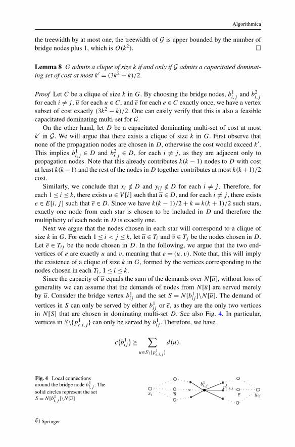
Next we argue that the nodes chosen in each star will correspond to a clique ofsize k in G. For each 1 ≤ i < j ≤ k, let u ∈ Ti and v ∈ Tj be the nodes chosen in D.Let e ∈ Tij be the node chosen in D. In the following, we argue that the two end-vertices of e are exactly u and v, meaning that e = (u, v). Note that, this will implythe existence of a clique of size k in G, formed by the vertices corresponding to thenodes chosen in each Ti , 1 ≤ i ≤ k.

Since the capacity of u equals the sum of the demands over N [u], without loss ofgenerality we can assume that the demands of nodes from N [u] are served merelyby u. Consider the bridge vertex b1

ij and the set S = N [b1ij ]\N [u]. The demand of

vertices in S can only be served by either b1ij or e, as they are the only two vertices

in N [S] that are chosen in dominating multi-set D. See also Fig. 4. In particular,vertices in S\{p1

e,i,j } can only be served by b1ij . Therefore, we have

c(b1ij

) ≥∑

u∈S\{p1e,i,j }

d(u).

Fig. 4 Local connectionsaround the bridge node b1

i,j. The

solid circles represent the setS = N [b1

i,j]\N [u]

Algorithmica

Since c(b1ij ) = ∑

u∈N [b1ij ] d(u) − N by our setting, the above inequality implies

d(p1e,i,j ) ≥ N − label(u), which in turn implies d(p2

e,i,j ) ≤ label(u) as we have

d(p1e,i,j ) + d(p2

e,i,j ) = N by our construction.

By a symmetric argument on b2i,j , we obtain d(p2

e,i,j ) ≥ label(u). Hence

d(p2e,i,j ) = label(u). By another symmetric argument on b1

ji and b2ji , we obtain

d(p2e,j,i ) = label(v). Therefore e = (u, v) and the lemma follows. �

Note that this proof holds for both separable and inseparable demand models. Wehave the following theorem.

Theorem 5 The capacitated domination problem is W [1]-hard when parameterizedby treewidth, regardless of the demand model.

Proof Clearly the reduction instance G can be computed in time polynomial in bothk and N . By Lemma 7, G has treewidth O(k2). This theorem follows directly fromLemma 8 and the W [1]-hardness of multicolored clique. �

We would like to remark that, from the construction of the graph G and the proofof Lemma 8, a feasible capacitated dominating multi-set with cost at most k′ for Galso has a cardinality of at most k′, and vice versa. Hence we have the followingcorollary.

Corollary 1 The capacitated domination problem is W [1]-hard when parameterizedby treewidth and solution size, regardless of the demand model.

Although we can state a stronger statement by incorporating the cardinality of thesolution size, i.e., the cardinality of the dominating multi-set as an extra parameter,knowing the solution size does not generally help us to obtain the demand assignmentfunction.

For example, consider the graph drawn in Fig. 5 with inseparable demands. Evenwhen we know that taking one multiplicity from each of v� and vr forms a feasibledominating multi-set, computing one of such demand assignment functions is stillNP-hard, by making a reduction from Partition, a well-known weakly NP-hard prob-lem. When the demand is separable, the computation can be done by using a standardflow algorithm. However, this does not give any guarantee on the cost of the resultingdemand assignment.

Fig. 5 A construction relatingthe computation of a feasibledemand assignment functionand the solution to the Partitionproblem when the demand isinseparable

Algorithmica

4.2 Fixed-Parameter Tractability w.r.t. Treewidth and Maximum Capacity

We have shown in the previous section that the capacitated domination problemis W [1]-hard, regardless of demand assignment model, when parameterized by thetreewidth of the input graph. In this section we show that, by taking the maxi-mum capacity as an extra parameter in addition to the treewidth, this problem be-comes fixed-parameter tractable when the demand is inseparable and can be solvedin O(22k((logM+1)+log k) · n) time, where M is the maximum capacity of the ver-tices.

To this end, we give a dynamic programming algorithm on a nice tree decompo-sition [34], which is a special tree decomposition, of the input graph. The advantageof this decomposition lies in the fact that it provides the structural information of thegiven graph in a well-organized fashion. Below we give a formal definition for thisconcept.

Definition 7 (Nice tree decomposition [34]) A tree decomposition

(X = {Xi : i ∈ I }, T = (I,F )

)

is a nice tree decomposition if one can root T in a way such that each node i ∈ I isof one of the following four types.

1. Leaf : node i is a leaf of T , and |Xi | = 1.2. Join: node i has exactly two children, say j1 and j2, and Xi = Xj1 = Xj2 .3. Introduce: node i has exactly one child, say j , and there is a vertex v ∈ V such

that Xi = Xj ∪ {v}.4. Forget: node i has exactly one child, say j , and there is a vertex v ∈ V such that

Xj = Xi ∪ {v}.

For a given tree decomposition of a graph with O(n) nodes and a bounded width,a nice tree decomposition of the same width can be found in O(n) time [34], wheren is the number of vertices.

Let G = (V ,E) be the input graph and (X ,T ) be a nice tree decomposition of G.For each node i ∈ T , let Ti be the subtree of T rooted at i and Yi := ⋃

j∈TiXj .

Literally, Yi denotes the set of vertices that are contained in the bags of the nodesin Ti .

Starting from the leaf nodes of T , our algorithm proceeds in a bottom-up mannerand maintains for each node i ∈ T a table Ai whose columns consist of the followinginformation.

– A subset of Xi indicating the set of vertices in Xi that have already been dominated,and

– for each u ∈ Xi , the amount of residue capacity of u, denoted rc(u), where 0 ≤rc(u) < c(u).

For each possible configuration of the columns described above, the algorithmwill maintain a row in Ai and computes the cost of the optimal demand assignment

Algorithmica

function for the subgraph induced by Yi under the condition that the set of verticesthat have been dominated by this demand assignment and also the residue capacityof each vertex meet exactly the values specified by the row. In order to help presentthe algorithm, for each row we store in the table Ai , say row r , we will refer to thecorresponding subset of Xi stored in row r by Pr .

In the following, we describe the computation of the table Ai for each node i inthe tree T . For the ease of presentation, we implicitly assumes that, whenever thealgorithm attempts to insert a new row into a table while another row with identicalconfiguration already exists, the one with the smaller cost will be kept. According todifferent types of vertices we encounter during the procedure, we have the followingfour cases.

– i is a leaf node. Let Xi = {v}. We add two rows to the table Ai which correspondto cases whether or not v is served.

1: let r1 = ({∅}, {rc(v) = 0}) be a new row with cost(r1) ←− 02: let r2 = ({v}, {rc(v) ≡ d(v) mod c(v)}) be a new row with

cost(r2) ←− w(v) · � d(v)c(v)

�3: add r1 and r2 to Ai

– i is an introduce node. Let j be the child of i, and let Xi = Xj ∪ {v}. The data inAj is inherited by Ai . We extend Ai by considering, for each existing row r in Aj ,all 2|Xj \Pr | possible ways of choosing vertices in Xj\Pr to be assigned to v. Inaddition, v can be either unassigned or assigned to any vertex in Xi . In either case,the cost and the residue capacity are modified accordingly.

1: for all rows r0 = (P,R) ∈ Aj do2: for all possible U such that U ⊆ (Xj\P) ∩ NG(v) do3: let R′ = R ∪ {rc(v) = ∑

u∈U d(u) mod c(v)}, andlet r = (P ∪ U,R′) be a new row with

cost(r) = cost(r0) + w(v) · �∑

u∈U d(u)

c(v)�

4: add r to Ai

5: for all u ∈ Xi do6: let r ′ = (P ∪ U ∪ {v},R′ ∪ {rc(u) = (rc(u) − d(v)) mod c(u)}) be a

new row withcost(r ′) = cost(r)+ the cost required by this assignment

7: add r ′ to Ai

8: end for9: end for

10: end for

– i is a forget node. Let j be the child of i, and let Xi = Xj\{v}. In this case, foreach row r ∈ Aj such that v ∈Pr , we insert a row r ′ to Ai identical to r except forthe absence of v in Pr ′ . The remaining rows in Aj , which correspond to situationswhere v is not served, are ignored without being considered.

Algorithmica

1: for all rows r0 = (P,R) ∈ Aj such that v ∈ P do2: let r = (P \{v},R\{rc(v)}) be a new row with cost(r) = cost(r0)

3: add r to Ai

4: end for

– i is a join node. Let j1 and j2 be the two children of i in T . We consider everypair of rows r1, r2 where r1 ∈ Aj1 and r2 ∈ Aj2 . We say that two rows r1 and r2 arecompatible if Pr1 ∩Pr2 = ∅. For each compatible pair of rows (r1, r2), we insert anew row r to Ai with Pr = Pr1 ∪Pr2 , rcr (u) = (rcr1(u) + rcr2(u)) mod c(u), for

each u ∈Xi , and cost(r) = cost(r1) + cost(r2) − ∑u∈Xi

rcr1 (u)+rcr2 (u)

c(u)�.

1: for all compatible pairs r1 = (P1,R1) ∈ Aj1 and r2 = (P2,R2) ∈ Aj2 do2: let r = (P1 ∪ P2,R) be a new row

3: cost(r) ←− cost(r1) + cost(r2) − ∑u∈Xi

rcR1 (u)+rcR2 (u)

c(u)�, and

4: R ←− {rcR1(u) + rcR2(u) mod c(u) : u ∈ Xi}5: add r to Ai

6: end for

Theorem 6 The capacitated domination problem with inseparable demand ongraphs of bounded treewidth can be solved in time 22k(logM+1)+log k+O(1) · n, wherek is the treewidth and M is the maximum capacity of the graph.

Proof The correctness of the algorithm follows from an inductive argument alongwith the description given above. Regarding the running time of this algorithm, firstnotice that the size of the table we maintained for each node of the tree decom-position is bounded by 2k · Mk . The computation for leaf nodes takes O(1) time,while the computation for introduce nodes and forget nodes take O(k22k · Mk) andO(2k · Mk), respectively. In join nodes, however, we consider each compatible pairof rows from two tables. Therefore the computation requires O(k22k · M2k) time.The size of a nice tree decomposition is linear in the number of vertices of thegraph. Therefore the overall running time of the algorithm is O(k22k · M2k · n) =22k(logM+1)+log k+O(1) · n. �

We state without going into details that, by suitably replacing the set Pi we main-tained for each row of the table Ai with the residue demand of each vertex containedin the bag Xi , the algorithm can be modified to handle separable demand model aswell. We have the following corollary.

Corollary 2 The capacitated domination problem with separable demand on graphsof bounded treewidth can be solved in time 2(2M+2N+1) log k+O(1) · n, where k is thetreewidth, M is the maximum capacity, and N is the maximum demand.

Algorithmica

5 A Constant-Factor Approximation for Outer-Planar Graphs with SeparableDemands

In this section, we develop an algorithm that computes a constant-factor approxi-mation for outerplanar graphs. In order to help present the algorithm and the finalanalysis in a systematic manner, we divide the entire section in the following way.

In Sect. 5.1, we present a structural statement that classifies the outer-planar graphsinto a class of graphs which we called general ladders, followed by showing how acorresponding representation can be extracted in O(n log3 n) time. In Sect. 5.2 wepresent a linear program, formerly introduced in [33], for this problem with separabledemands. In Sect. 5.3 we consider the primal linear program and propose a scheme toreduce the structure of the general ladders we introduce in Sect. 5.1. Then in Sect. 5.4we consider the dual program of the relaxation of the linear program to obtain aconstant-factor approximation for the reduced subgraph.

To give an exact idea on how the algorithm works, for any outerplanar graphG = (V ,E), our algorithm proceeds as follows. First we use the algorithm describedin Sect. 5.1 to compute a general ladder representation of G and a decomposition intothree subproblems, denoted G0, G1, and G2. For each subproblem Gi , 0 ≤ i < 3, weuse the approach described in Sect. 5.3 to further reduce its structure and to obtaina reduced subgraph Hi . For each of the reduced subgraph Hi , we apply the algo-rithm described in Sect. 5.4 to obtain an approximation, represented by a demand as-signment function fi . The overall approximation for G, i.e., the demand assignmentfunction f , is defined to be f = ∑

0≤i<3 fi . An overall analysis of this algorithm isgiven in Sect. 5.5.

5.1 General Ladders and Outerplanar Graphs

First we define the notation which we will use later on. By a total order of a setwe mean that each pair of elements in the set can be compared, and therefore anascending order of the elements is well-defined. Let P = (v1, v2, . . . , vk) be a path.We say that P is an ordered path if a total order v1 ≺ v2 ≺ · · · ≺ vk or vk ≺ vk−1 ≺· · · ≺ v1 is defined on the set of vertices. Note that, provided the notion of total orders,the concepts of maximum elements and minimum elements naturally extends, i.e., forany finite set A with a total order defined, we have minx∈A x � y � maxx∈A x for ally ∈ A.

Definition 8 (General ladder) A graph G = (V ,E) is said to be a general ladder ifa total order on the set of vertices is defined, and G is composed of a set of layers{L1,L2, . . . ,Lk}, where each layer is a collection of subpaths of an ordered pathsuch that the following holds. The top layer, L1, consists of a single vertex, which isreferred to as the anchor, and for each 1 < j < k and u,v ∈ Lj , we have (1) N [u] ⊆Lj−1 ∪Lj ∪Lj+1, and (2) u ≺ v implies maxp∈N [u]∩Lj+1 p � minq∈N [v]∩Lj+1 q .

Note that each layer in a general ladder consists of a set of ordered paths which arepossibly connected only to vertices in the neighboring layers. See Fig. 6(a). Althoughthe definition of general ladders captures the essence and simplicity of an ordered

Algorithmica

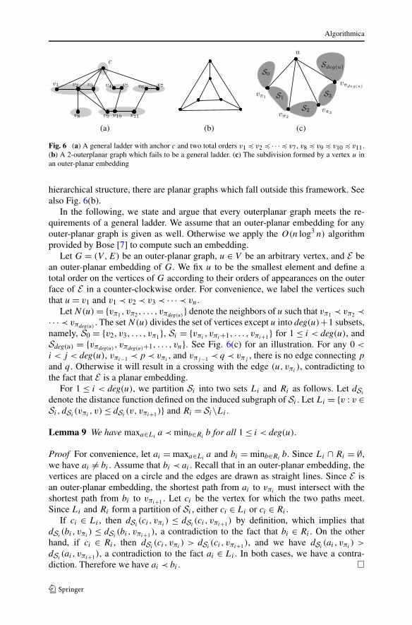
Fig. 6 (a) A general ladder with anchor c and two total orders v1 � v2 � · · · � v7, v8 � v9 � v10 � v11.(b) A 2-outerplanar graph which fails to be a general ladder. (c) The subdivision formed by a vertex u inan outer-planar embedding

hierarchical structure, there are planar graphs which fall outside this framework. Seealso Fig. 6(b).

In the following, we state and argue that every outerplanar graph meets the re-quirements of a general ladder. We assume that an outer-planar embedding for anyouter-planar graph is given as well. Otherwise we apply the O(n log3 n) algorithmprovided by Bose [7] to compute such an embedding.

Let G = (V ,E) be an outer-planar graph, u ∈ V be an arbitrary vertex, and E bean outer-planar embedding of G. We fix u to be the smallest element and define atotal order on the vertices of G according to their orders of appearances on the outerface of E in a counter-clockwise order. For convenience, we label the vertices suchthat u = v1 and v1 ≺ v2 ≺ v3 ≺ · · · ≺ vn.

Let N(u) = {vπ1, vπ2 , . . . , vπdeg(u)} denote the neighbors of u such that vπ1 ≺ vπ2 ≺

· · · ≺ vπdeg(u). The set N(u) divides the set of vertices except u into deg(u)+1 subsets,

namely, S0 = {v2, v3, . . . , vπ1}, Si = {vπi, vπi+1, . . . , vπi+1} for 1 ≤ i < deg(u), and

Sdeg(u) = {vπdeg(u), vπdeg(u)+1, . . . , vn}. See Fig. 6(c) for an illustration. For any 0 <

i < j < deg(u), vπi−1 ≺ p ≺ vπi, and vπj−1 ≺ q ≺ vπj

, there is no edge connecting p

and q . Otherwise it will result in a crossing with the edge (u, vπi), contradicting to

the fact that E is a planar embedding.For 1 ≤ i < deg(u), we partition Si into two sets Li and Ri as follows. Let dSi

denote the distance function defined on the induced subgraph of Si . Let Li = {v : v ∈Si , dSi

(vπi, v) ≤ dSi

(v, vπi+1)} and Ri = Si\Li .

Lemma 9 We have maxa∈Lia ≺ minb∈Ri

b for all 1 ≤ i < deg(u).

Proof For convenience, let ai = maxa∈Lia and bi = minb∈Ri

b. Since Li ∩ Ri = ∅,we have ai �= bi . Assume that bi ≺ ai . Recall that in an outer-planar embedding, thevertices are placed on a circle and the edges are drawn as straight lines. Since E isan outer-planar embedding, the shortest path from ai to vπi

must intersect with theshortest path from bi to vπi+1 . Let ci be the vertex for which the two paths meet.Since Li and Ri form a partition of Si , either ci ∈ Li or ci ∈ Ri .

If ci ∈ Li , then dSi(ci , vπi

) ≤ dSi(ci , vπi+1) by definition, which implies that

dSi(bi , vπi

) ≤ dSi(bi, vπi+1), a contradiction to the fact that bi ∈ Ri . On the other

hand, if ci ∈ Ri , then dSi(ci , vπi

) > dSi(ci , vπi+1), and we have dSi

(ai , vπi) >

dSi(ai , vπi+1), a contradiction to the fact ai ∈ Li . In both cases, we have a contra-

diction. Therefore we have ai ≺ bi . �

Algorithmica

Fig. 7 (a) A contradiction led by minb∈Rib ≺ maxa∈Li

a. (b) Partition of Si into Li and Ri

Let �(v) := dG(u, v) denote the distance between v and the anchor u in G. Let�i(v) := min{dSi

(vπ(i), v), dSi

(vπ(i+1), v)}, for any 1 ≤ i < deg(u) and v ∈ Si . Ob-

serve that �(v) = �i(v) + 1, for any 1 ≤ i < deg(u) and v ∈ Si . Now consider theset of the edges connecting Li and Ri . Note that, this is exactly the set of edgesconnecting vertices on the shortest path between vπi

and maxa∈Lia and vertices on

the shortest path between vπi+1 and minb∈Rib. We have the following lemma, which

states that, when the vertices are classified by their distances to u, these edges canonly connect vertices between neighboring sets and do not form any crossing. Seealso Fig. 7.

Lemma 10 For any edge (p, q), p ∈ Li , q ∈ Ri , connecting Li and Ri , we have

– |�(p) − �(q)| ≤ 1, and– � edge (r, s), (r, s) �= (p, q), r ∈ Li , s ∈ Ri , such that �(r) = �(q) and �(p) = �(s).

Proof The first half of the lemma follows from the definition of �. If|�(p) − �(q)| > 1, without loss of generality, suppose that �(p) > �(q)+ 1, by goingthrough (p, q) then following the shortest path from q to u, we find a shorter pathfor p, which is a contradiction. The second half follows from the fact that E is aplanar embedding. �

Now we are ready to state the structural property.

Lemma 11 Any outer-planar graph G = (V ,E) together with an arbitrary vertexu ∈ V is a general ladder anchored at u, where the set of vertices in each layer areclassified by their distances to the anchor u.

Proof We prove by induction on the number of vertices of G. First, an isolated vertexis a single-layer general ladder. For non-trivial graphs, let S0,S1, . . . ,Sdeg(u) be thesubsets defined as above. By assumption, the induced subgraphs of S0 and Sdeg(u) aregeneral ladders with anchors vπ1 and vπdeg(u)

, respectively. Furthermore, the layers areclassified by � − 1. That is, vertex v belongs to layer �(v) − 1. Similarly, the inducedsubgraphs of Li and Ri are also general ladders with anchors vπi

and vπi+1 whoselayers are classified by �i .

Now we argue that these general ladders can be arranged properly to form asingle general ladder with anchor u and layers classified by �. Since there is noedge connecting p and q for any p,q with vπi−1 ≺ p ≺ vπi

and vπj−1 ≺ q ≺ vπj,

Algorithmica

0 < i < j < deg(u), we only need to consider the edges connecting vertices betweenLi and Ri . By Lemma 10, when the general ladders Li and Ri are hung over vπi

and vπi+1 , respectively, the edges between them connect exactly only vertices fromadjacent layers and do not form any crossing. Therefore, it forms a general ladderwith u being the anchor and the lemma follows. �

5.1.1 Extracting the general ladder

Let G = (V ,E) be the input outer-planar graph and u ∈ V be an arbitrary vertex. Wecan extract the corresponding general ladder in linear time.

Theorem 7 Given an outer-planar graph G and its outer-planar embedding, we cancompute in linear time a general ladder representation for G.

Proof First we compute the shortest distance from each vertex v ∈ V to u. Denote theshortest distance by �(v). Since the number of edges in a planar graph is linear in thenumber of vertices, the computation can be done by a standard breadth-first-search(BFS) algorithm and takes time linear in the number of vertices.

Let M = maxv∈V �(v). We create M+1 empty queues, denoted layer0, layer1, . . . ,

layerM . The queues will be used to maintain the set of layers. We traverse the verticesof G, starting from u, in a counter-clockwise order according to the given embedding.For each vertex v visited, we attach v to the end of layer�(v). The traversal of the outerface takes linear time. The correctness of this approach is assured by Lemma 11. �

For the rest of this paper we will denote the layers of this particular general lad-der representation by L0,L1, . . . ,LM . The following additional structural propertycomes from the outer-planarity of G and our construction scheme.

Lemma 12 For any 0 < i ≤ M and v ∈ Li , we have |N(v) ∩ Li−1| ≤ 2. Moreover,if v has two neighbors in Li , say, v1 and v2 with v1 ≺ v ≺ v2, then there is an edgejoining v1 (and v2, respectively) and each neighboring vertex of v in Li−1 that issmaller (larger) than v.

Proof First, since the layers are classified by the distances to the anchor u, if |N(v)∩Li−1| ≥ 3, then consider the shortest paths from vertices in N(v)∩Li−1 to u. At leastone vertex would be surrounded by another two paths, contradicting the fact that G isan outer-planar graph.

The second part is obtained from a similar argument. Let v′ ∈ N(v) ∩ Li−1 be aneighbor of v in Li−1. If v′ is not joined to either v1 or v2, then consider the shortestpaths from u to v1, v′, and v2, respectively. v′ would be a vertex in the interior, whichis a contradiction. �

The Decomposition The idea behind this decomposition is to help reduce the depen-dency between vertices of large degrees and their neighbors such that further tech-niques can be applied. To this end, we tackle the demands of vertices from every threelayers separately.

Algorithmica

For each 0 ≤ i < 3, let Ri = ⋃j≥0 L3j+i . Let Gi = (Vi,Ei) consist of the induced

subgraph of Ri and the set of edges connecting vertices in Ri to their neighbors.Formally, Vi = ⋃

v∈RiN [v] and Ei = ⋃

v∈Ri

⋃u∈N [v] e(u, v). In addition, we set

d(v) = 0 for all v ∈ Gi\Ri . Other parameters remain unchanged.

Lemma 13 Let fi , 0 ≤ i < 3, be an optimal demand assignment function for Gi . Theassignment function f = ∑

0≤i<3 fi is a 3-approximation of G.

Proof First, for any vertex v ∈ V , the demand of v is considered in Gi for some0 ≤ i < 3 and therefore is assigned by the assignment function fi . Since we take theunion of the three assignments, it is a feasible assignment to the entire graph G.

Since the demand of each vertex in Gi , 0 ≤ i < 3, is no more than that of in theoriginal graph G, any feasible solution to G will also serve as a feasible solution to Gi .Therefore we have OPT(Gj ) ≤ OPT(G), for 0 ≤ j < 3, and the lemma follows. �

5.2 A Linear Program for the Separable Demand Model

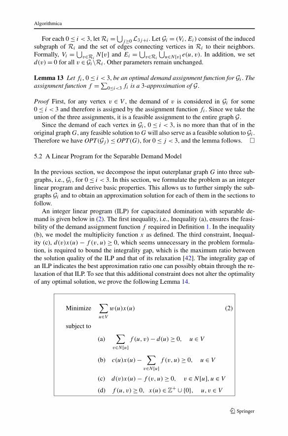
In the previous section, we decompose the input outerplanar graph G into three sub-graphs, i.e., Gi , for 0 ≤ i < 3. In this section, we formulate the problem as an integerlinear program and derive basic properties. This allows us to further simply the sub-graphs Gi and to obtain an approximation solution for each of them in the sections tofollow.

An integer linear program (ILP) for capacitated domination with separable de-mand is given below in (2). The first inequality, i.e., Inequality (a), ensures the feasi-bility of the demand assignment function f required in Definition 1. In the inequality(b), we model the multiplicity function x as defined. The third constraint, Inequal-ity (c), d(v)x(u) − f (v,u) ≥ 0, which seems unnecessary in the problem formula-tion, is required to bound the integrality gap, which is the maximum ratio betweenthe solution quality of the ILP and that of its relaxation [42]. The integrality gap ofan ILP indicates the best approximation ratio one can possibly obtain through the re-laxation of that ILP. To see that this additional constraint does not alter the optimalityof any optimal solution, we prove the following Lemma 14.

Minimize∑

u∈V

w(u)x(u) (2)

subject to

(a)∑

v∈N [u]f (u, v) − d(u) ≥ 0, u ∈ V

(b) c(u)x(u) −∑

v∈N [u]f (v,u) ≥ 0, u ∈ V

(c) d(v)x(u) − f (v,u) ≥ 0, v ∈ N [u], u ∈ V

(d) f (u, v) ≥ 0, x(u) ∈ Z+ ∪ {0}, u, v ∈ V

Algorithmica

Lemma 14 Let f be an arbitrary optimal demand assignment function. We haved(v) · xf (u) − f (v,u) ≥ 0 for all u ∈ V and v ∈ N [u].

Proof Without loss of generality, we may assume that d(v) ≥ f (v,u). Otherwise,we set f (v,u) to be d(v) and the resulting assignment would be feasible and thecost can only be better. If xf (u) = 0, then we have f (v,u) = 0 by definition, andthis inequality holds trivially. Otherwise, if xf (u) ≥ 1, then d(v) · xf (u) − f (v,u) ≥f (v,u) · (xf (u) − 1) ≥ 0. �

However, without this constraint, the integrality gap can be arbitrarily large. Thisis illustrated by the following example. Let α > 1 be an arbitrary constant, and T (α)

be an n-vertex star, where each vertex has unit demand and unit cost. The capacity ofthe central vertex is set to be n, which is sufficient to cover the demand of the entiregraph, while the capacity of each of remaining n − 1 petal vertices is set to be αn.

Lemma 15 Without the additional constraint d(v)x(u)−f (v,u) ≥ 0, the integralitygap of the ILP (2) on T (α) is α, where α > 1 is an arbitrary constant.

Proof The optimal dominating set consists of a single multiplicity of the central ver-tex with unit cost, while the optimal fractional solution is formed by spending 1

αnmultiplicity at a petal vertex for each unit demand from the vertices of this graph,making an overall cost of 1

αand therefore an arbitrarily large integrality gap. �

Indeed, with the additional constraint applied, we can refrain from unreasonablyassigning a small amount of demand to any vertex in any fractional solution. Takea petal vertex, say v, from T (α) as example, given that d(v) = 1 and f (v, v) = 1,this constraint would force x(v) to be at least 1, which prevents the aforementionedsituation from being an optimal fractional solution.

For the rest of this paper, for any graph G, we denote the optimal values to the in-teger linear program (2) and to its relaxation by OPT(G) and OPTf (G), respectively.Note that OPTf (G) ≤ OPT(G).

5.3 Reducing the General Ladder

In this section we describe an approach to further simplifying the subgraphs Gi weobtained from the decomposition of the input graph G proposed in Sect. 5.1, for0 ≤ i < 3. Given any feasible demand assignment for Gi , we can properly reassignthe demand of a vertex to a constant number of neighbors while the increase in termsof fractional cost remains bounded.

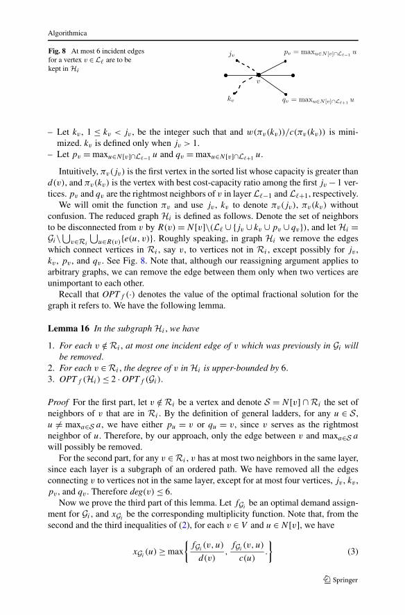
For each v ∈ Ri , we sort the closed neighbors of v according to their cost inascending order such that w(πv(1)) ≤ w(πv(2)) ≤ · · · ≤ w(πv(deg[v])), where πv :{1,2, . . . ,deg[v]} → N [v] is an injective function. For convenience, we implicitlyextend the domain of πv and set πv(deg[v]+ 1) = ∅ as a dummy entity. Suppose thatv ∈ L�. We identify the following four vertices.

– Let jv , 1 ≤ jv ≤ deg[v], be the smallest integer such that c(πv(jv)) > d(v). Ifc(πv(j)) ≤ d(v) for all 1 ≤ j ≤ deg[v], then we let jv = deg[v] + 1.

Algorithmica

Fig. 8 At most 6 incident edgesfor a vertex v ∈ L� are to bekept in Hi

– Let kv , 1 ≤ kv < jv , be the integer such that and w(πv(kv))/c(πv(kv)) is mini-mized. kv is defined only when jv > 1.

– Let pv = maxu∈N [v]∩L�−1 u and qv = maxu∈N [v]∩L�+1 u.

Intuitively, πv(jv) is the first vertex in the sorted list whose capacity is greater thand(v), and πv(kv) is the vertex with best cost-capacity ratio among the first jv −1 ver-tices. pv and qv are the rightmost neighbors of v in layer L�−1 and L�+1, respectively.

We will omit the function πv and use jv , kv to denote πv(jv), πv(kv) withoutconfusion. The reduced graph Hi is defined as follows. Denote the set of neighborsto be disconnected from v by R(v) = N [v]\(L� ∪ {jv ∪ kv ∪ pv ∪ qv}), and let Hi =Gi\⋃

v∈Ri

⋃u∈R(v){e(u, v)}. Roughly speaking, in graph Hi we remove the edges

which connect vertices in Ri , say v, to vertices not in Ri , except possibly for jv ,kv , pv , and qv . See Fig. 8. Note that, although our reassigning argument applies toarbitrary graphs, we can remove the edge between them only when two vertices areunimportant to each other.

Recall that OPTf (·) denotes the value of the optimal fractional solution for thegraph it refers to. We have the following lemma.

Lemma 16 In the subgraph Hi , we have

1. For each v /∈ Ri , at most one incident edge of v which was previously in Gi willbe removed.

2. For each v ∈Ri , the degree of v in Hi is upper-bounded by 6.3. OPTf (Hi ) ≤ 2 · OPTf (Gi ).

Proof For the first part, let v /∈ Ri be a vertex and denote S = N [v] ∩ Ri the set ofneighbors of v that are in Ri . By the definition of general ladders, for any u ∈ S ,u �= maxa∈S a, we have either pu = v or qu = v, since v serves as the rightmostneighbor of u. Therefore, by our approach, only the edge between v and maxa∈S a

will possibly be removed.For the second part, for any v ∈ Ri , v has at most two neighbors in the same layer,

since each layer is a subgraph of an ordered path. We have removed all the edgesconnecting v to vertices not in the same layer, except for at most four vertices, jv , kv ,pv , and qv . Therefore deg(v) ≤ 6.

Now we prove the third part of this lemma. Let fGibe an optimal demand assign-

ment for Gi , and xGibe the corresponding multiplicity function. Note that, from the

second and the third inequalities of (2), for each v ∈ V and u ∈ N [v], we have

xGi(u) ≥ max

{fGi

(v, u)

d(v),fGi

(v, u)

c(u).

}(3)

Algorithmica

For each v ∈Ri and u ∈ R(v) such that fGi(v, u) �= 0, we modify this assignment

as follows. If π−1v (u) ≥ jv , then we assign it to jv instead of to u. Otherwise, we

assign it to kv . That is, depending on whether π−1v (u) ≥ jv , we raise either fGi

(v, jv)

or fGi(v, kv) by the amount of fGi

(v, u) and then set fGi(v, u) to be zero. Note

that, after this reassignment, the modified assignment function fGiwill be a feasible

assignment for Hi as well.In order to cope with this change, xGi

(jv) or xGi(kv) might have to be raised as

well until both the second and the third inequalities are valid again. If π−1v (u) ≥ jv ,

then xGi(jv) is raised by at most

max{fGi

(v, u)/d(v), fGi(v, u)/c(jv)

},

which is equal to fGi(v, u)/d(v), since c(jv) > d(v). Hence the total cost will be

raised by at most

w(jv) · fGi(v, u)

d(v)≤ w(jv) · max

{fGi

(v, u)

d(v),fGi

(v, u)

c(u)

}≤ w(u) · xGi

(u),

by Inequality (3) and the fact that w(jv) ≤ w(u). Similarly, if π−1v (u) < jv , the cost

is raised by at most

w(kv) · max

{fGi

(v, u)

d(v),fGi

(v, u)

c(kv)

}= w(kv) · fGi

(v, u)

c(kv)

≤ w(u) · fGi(v, u)

c(u)≤ w(u) · xGi

(u),

since we have w(kv)c(kv)

≤ w(u)c(u)

by definition of kv and Inequality (3).In both cases, the extra cost required by this specific demand reassignment be-

tween v and u is bounded by w(u) · xGi(u). By the first part of this lemma, we have

at most one such pair for each u /∈ Ri , the overall cost is at most doubled and thislemma follows. �

We also remark that, although OPTf (Hi ) is bounded in terms of OPTf (Gi ), anα-approximation for Hi is not necessarily a 2α-approximation for Gi . That is, havingan approximation A with OPT(A) ≤ α · OPT(Hi ) does not imply that OPT(A) ≤2α ·OPT(Gi ), for OPT(Hi ) could be strictly larger than OPTf (Hi ). Instead, to obtainour claimed result, an approximation with a stronger bound, in terms of OPTf (Hi ),is desired.

5.4 Greedy Charging Scheme

We show how we can further approximate the optimal solution for the reduced graphHi by a sophisticated primal-dual charging argument. Let Vi be the vertex set of Hi .We apply a technique from [33] to obtain a feasible solution for the dual program ofthe relaxation of the ILP (2) from Sect. 5.2, which is given below in (4).

It is not difficult to see that the linear program (4) is exactly a packing program,i.e., a linear program whose objective is to pack “items” subject to certain “space”

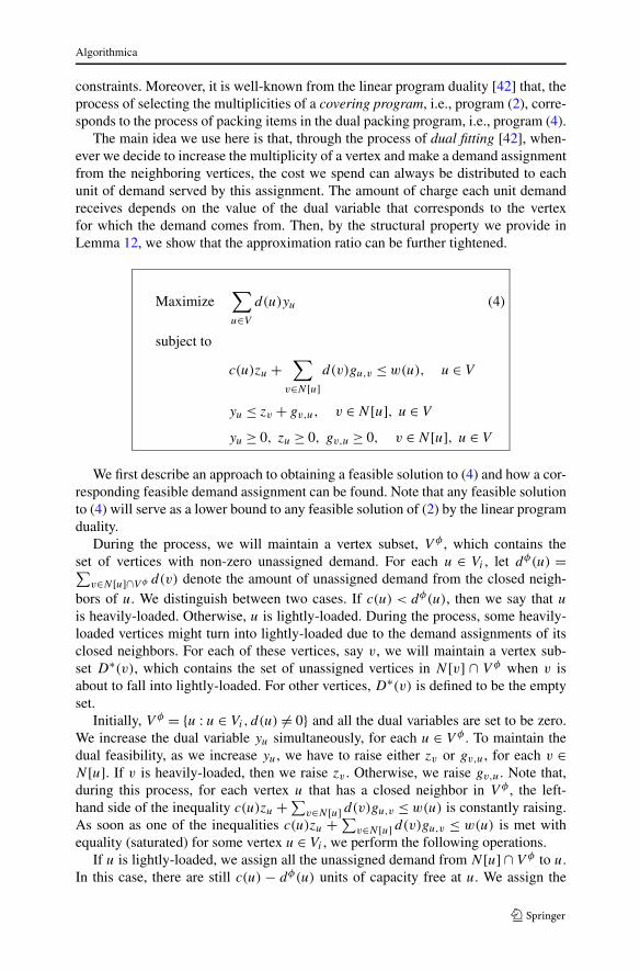
Algorithmica

constraints. Moreover, it is well-known from the linear program duality [42] that, theprocess of selecting the multiplicities of a covering program, i.e., program (2), corre-sponds to the process of packing items in the dual packing program, i.e., program (4).

The main idea we use here is that, through the process of dual fitting [42], when-ever we decide to increase the multiplicity of a vertex and make a demand assignmentfrom the neighboring vertices, the cost we spend can always be distributed to eachunit of demand served by this assignment. The amount of charge each unit demandreceives depends on the value of the dual variable that corresponds to the vertexfor which the demand comes from. Then, by the structural property we provide inLemma 12, we show that the approximation ratio can be further tightened.

Maximize∑

u∈V

d(u)yu (4)

subject to

c(u)zu +∑

v∈N [u]d(v)gu,v ≤ w(u), u ∈ V

yu ≤ zv + gv,u, v ∈ N [u], u ∈ V

yu ≥ 0, zu ≥ 0, gv,u ≥ 0, v ∈ N [u], u ∈ V

We first describe an approach to obtaining a feasible solution to (4) and how a cor-responding feasible demand assignment can be found. Note that any feasible solutionto (4) will serve as a lower bound to any feasible solution of (2) by the linear programduality.

During the process, we will maintain a vertex subset, V φ , which contains theset of vertices with non-zero unassigned demand. For each u ∈ Vi , let dφ(u) =∑

v∈N [u]∩V φ d(v) denote the amount of unassigned demand from the closed neigh-bors of u. We distinguish between two cases. If c(u) < dφ(u), then we say that u

is heavily-loaded. Otherwise, u is lightly-loaded. During the process, some heavily-loaded vertices might turn into lightly-loaded due to the demand assignments of itsclosed neighbors. For each of these vertices, say v, we will maintain a vertex sub-set D∗(v), which contains the set of unassigned vertices in N [v] ∩ V φ when v isabout to fall into lightly-loaded. For other vertices, D∗(v) is defined to be the emptyset.

Initially, V φ = {u : u ∈ Vi, d(u) �= 0} and all the dual variables are set to be zero.We increase the dual variable yu simultaneously, for each u ∈ V φ . To maintain thedual feasibility, as we increase yu, we have to raise either zv or gv,u, for each v ∈N [u]. If v is heavily-loaded, then we raise zv . Otherwise, we raise gv,u. Note that,during this process, for each vertex u that has a closed neighbor in V φ , the left-hand side of the inequality c(u)zu + ∑

v∈N [u] d(v)gu,v ≤ w(u) is constantly raising.As soon as one of the inequalities c(u)zu + ∑

v∈N [u] d(v)gu,v ≤ w(u) is met withequality (saturated) for some vertex u ∈ Vi , we perform the following operations.

If u is lightly-loaded, we assign all the unassigned demand from N [u] ∩ V φ to u.In this case, there are still c(u) − dφ(u) units of capacity free at u. We assign the

Algorithmica

ALGORITHM Greedy-Charging

1: V φ ←− {u : u ∈ Vi, d(u) �= 0}, V ∗ ←− Vi .2: dφ(u) ←− ∑

v∈N [u] d(v), for each u ∈ Vi .

3: wφ(u) ←− w(u), for each u ∈ V .4: Let Q be a first-in-first-out queue.5: while V φ �= ∅ do6: rv ←− wφ(v)/min{c(v), dφ(v)}, for each v ∈ V ∗.7: u ←− arg min{rv : v ∈ V ∗}. [u is the next vertex to be saturated.]8: wφ(v) ←− wφ(v) − wφ(u), for each v ∈ V ∗.9:

10: if dφ(u) ≤ c(u) then11: Assign the demand from N [u] ∩ V φ to u.12: Assign c(u) − dφ(u) amount of unassigned demand from D∗(u), if there is any, to u.13: else14: Attach u to the queue Q and mark u as heavy.15: end if16: Let Su ←− (N [u] ∩ V φ) ∪ {u}.17: Remove N [u] from V φ and update the corresponding dφ(v) for v ∈ Vi .18: For each v ∈ V ∗ such that dφ(v) = 0, remove v from V ∗ .19: for all vertex v becomes lightly-loaded in this iteration do20: D∗(v) ←− N [v] ∩ (V φ ∪ Su).21: end for22: end while23: while Q �= ∅ do24: Extract a vertex from the head of Q, say u.25: Assign the unassigned demand from N [u] to u.26: end while27:

Fig. 9 A high-level pseudo-code for the primal-dual algorithm

unassigned demand from D∗(u), if there is any, to u until either all the demand fromD∗(u) is assigned or all the free capacity in u is used. On the other hand, if u isheavily-loaded, we mark it as heavy and delay the demand assignment from its closedneighbors.

Then we set Qu = N [u] ∩ V φ and remove N [u] from V φ . Note that, due to thedefinition of dφ , even when u is heavily-loaded, we still update dφ(p) for each p ∈ Vi

with N [p] ∩ N [u] �= ∅, if needed, as if the demand was assigned. During the aboveoperation, some heavily-loaded vertices might turn into lightly-loaded due to the de-mand assignments (or simply due to the update of dφ). For each of these vertices,say v, we set D∗(v) = N [v] ∩ (V φ ∪ Qu). Intuitively, D∗(v) contains the set ofunassigned vertices from N [v] ∩ V φ when v is about to fall into the lightly-loadedvertices.

This process continues until V φ = ∅. For those vertices which are marked asheavy, we iterate over them according to their chronological order of being saturatedand assign at this moment all the remaining unassigned demand from their closedneighbors to them. A high-level description of this algorithm is provided in Fig. 9.

Let f ∗ : V ×V → R+ ∪{0} denote the resulting demand assignment function, andx∗ : V → Z+ ∪ {0} denotes the corresponding multiplicity function. The followinglemma bounds the cost of the solution produced by our algorithm.

Algorithmica

Lemma 17 For any Hi obtained from a general ladder Gi , we have w(f ∗) ≤ 7 ·OPTf (Hi ).

Proof We argue in the following that, for each u ∈ Vi , the cost resulted by u, which isw(u) · x∗(u), can be distributed to a certain portion of the demands from the verticesin N [u] such that each unit demand, say from vertex v ∈ N [u], receives a charge ofat most 7 · yv .

Let u ∈ Vi be a vertex with x∗(u) > 0. If u has been marked as heavy, then by ourscheme, we have gu,v = 0 and yv = zu for all v ∈ N [u]. Therefore w(u) = c(u) ·zu =c(u) · yv , and for each multiplicity of u, we need c(u) units of demand from N [u].If x∗(u) > 1, then at least c(u) · (x∗(u) − 1) units of demand are assigned to u, andby distributing the cost to them, each unit of demand gets charged at most twice. Ifx∗(u) = 1, then we charge the cost to any c(u) units of demand that are counted indφ(u) when u is saturated. Since u is a heavily-loaded vertex, dφ(u) > c(u) and therewill be sufficient amount of demand to charge.

If u is lightly-loaded, then x∗(u) = 1 and we have two cases. First, if∑v∈N [u] d(v) ≤ c(u), then u is lightly-loaded in the beginning and we have zu = 0

and yv = gu,v for each v ∈ N [u], which implies

w(u) =∑

v∈N [u]d(v) · gu,v =

∑

v∈N [u]d(v) · yv.

The cost w(u) of u can be distributed to all the demand from its closed neighbors,each unit demand, say from vertex v ∈ N [u], gets a charge of yv .

If∑

v∈N [u] d(v) > c(u), then u is heavily-loaded in the beginning and at somepoint turned into lightly-loaded. Let U0 ⊆ D∗(u) be the set of vertices whose removalfrom V φ achieves this change. By our scheme, zu is raised in the beginning and atsome point when dφ(u) is about to fall below c(u), we fix zu and start raising gu,v

for v ∈ D∗(u)\U0. Note that we have⎧⎪⎨

⎪⎩

yu0 = zu for all u0 ∈ U0,

yv = zu + gu,v for each v ∈ D∗(u)\U0, and

gu,v = 0 for v ∈ (N [u]\D∗(u)) ∪ U0.

Let d∗U0

= c(u) − ∑v∈D∗(u)\U0

d(v). We have

w(u) = c(u) · zu +∑

v∈N [u]d(v) · gu,v

=(

d∗U0

+∑

v∈D∗(u)\U0

d(v)

)· zu +

∑

v∈D∗(u)

d(v) · gu,v

= d∗U0

· zu +∑

v∈D∗(u)\U0

d(v) · (zu + gu,v)

≤∑

v∈U0

dv · yv +∑

v∈D∗(u)\U0

d(v) · yv.

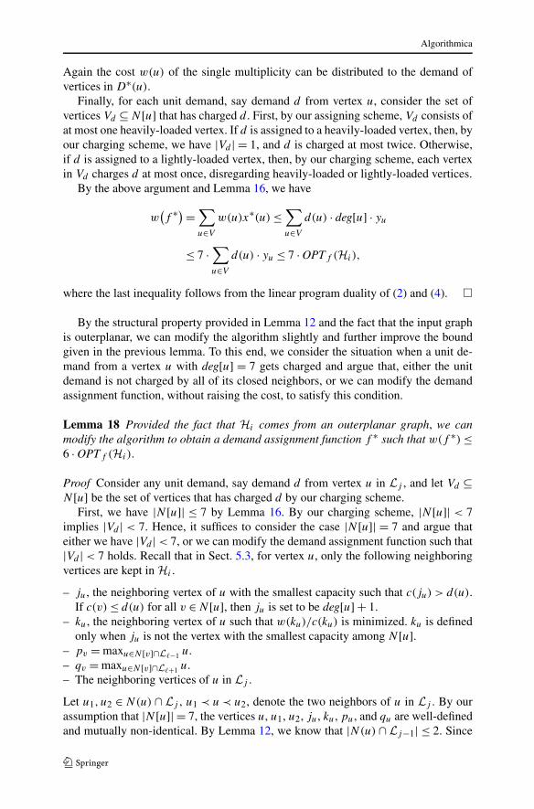
Algorithmica

Again the cost w(u) of the single multiplicity can be distributed to the demand ofvertices in D∗(u).

Finally, for each unit demand, say demand d from vertex u, consider the set ofvertices Vd ⊆ N [u] that has charged d . First, by our assigning scheme, Vd consists ofat most one heavily-loaded vertex. If d is assigned to a heavily-loaded vertex, then, byour charging scheme, we have |Vd | = 1, and d is charged at most twice. Otherwise,if d is assigned to a lightly-loaded vertex, then, by our charging scheme, each vertexin Vd charges d at most once, disregarding heavily-loaded or lightly-loaded vertices.

By the above argument and Lemma 16, we have

w(f ∗) =

∑

u∈V

w(u)x∗(u) ≤∑

u∈V

d(u) · deg[u] · yu

≤ 7 ·∑

u∈V

d(u) · yu ≤ 7 · OPTf (Hi ),

where the last inequality follows from the linear program duality of (2) and (4). �

By the structural property provided in Lemma 12 and the fact that the input graphis outerplanar, we can modify the algorithm slightly and further improve the boundgiven in the previous lemma. To this end, we consider the situation when a unit de-mand from a vertex u with deg[u] = 7 gets charged and argue that, either the unitdemand is not charged by all of its closed neighbors, or we can modify the demandassignment function, without raising the cost, to satisfy this condition.

Lemma 18 Provided the fact that Hi comes from an outerplanar graph, we canmodify the algorithm to obtain a demand assignment function f ∗ such that w(f ∗) ≤6 · OPTf (Hi ).

Proof Consider any unit demand, say demand d from vertex u in Lj , and let Vd ⊆N [u] be the set of vertices that has charged d by our charging scheme.

First, we have |N [u]| ≤ 7 by Lemma 16. By our charging scheme, |N [u]| < 7implies |Vd | < 7. Hence, it suffices to consider the case |N [u]| = 7 and argue thateither we have |Vd | < 7, or we can modify the demand assignment function such that|Vd | < 7 holds. Recall that in Sect. 5.3, for vertex u, only the following neighboringvertices are kept in Hi .

– ju, the neighboring vertex of u with the smallest capacity such that c(ju) > d(u).If c(v) ≤ d(u) for all v ∈ N [u], then ju is set to be deg[u] + 1.

– ku, the neighboring vertex of u such that w(ku)/c(ku) is minimized. ku is definedonly when ju is not the vertex with the smallest capacity among N [u].

– pv = maxu∈N [v]∩L�−1 u.– qv = maxu∈N [v]∩L�+1 u.– The neighboring vertices of u in Lj .

Let u1, u2 ∈ N(u) ∩ Lj , u1 ≺ u ≺ u2, denote the two neighbors of u in Lj . By ourassumption that |N [u]| = 7, the vertices u, u1, u2, ju, ku, pu, and qu are well-definedand mutually non-identical. By Lemma 12, we know that |N(u) ∩ Lj−1| ≤ 2. Since

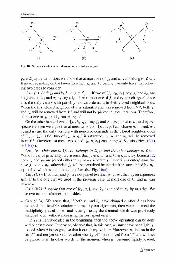
Algorithmica

Fig. 10 Situations when a unit demand of u is fully-charged

pu ∈ Lj−1 by definition, we know that at most one of ju and ku can belong to Lj−1.Hence, depending on the layers to which ju and ku belong, we only have the follow-ing two cases to consider.

Case (a): Both ju and ku belong to Lj+1. If two of {ju, ku, qu}, say, ju and ku, arenot joined to u1 and u2 by any edge, then at most one of ju and ku can charge d , sinceu is the only vertex with possibly non-zero demand in their closed neighborhoods.When the first closed neighbor of u is saturated and u is removed from V φ , both ju

and ku will be removed from V ∗ and will not be picked in later iterations. Therefore,at most one of ju and ku can charge d .

On the other hand, if two of {ju, ku, qu}, say ju and qu, are joined to u1 and u2, re-spectively, then we argue that at most two out of {ju,u, qu} can charge d . Indeed, u1,u, and u2 are the only vertices with non-zero demands in the closed neighborhoodsof {ju,u, qu}. After two of {ju,u, qu} is saturated, u1, u, and u2 will be removedfrom V φ . Therefore, at most two out of {ju,u, qu} can charge d . See also Figs. 10(a)and 10(b).

Case (b): Only one of {ju, ku} belongs to Lj+1 and the other belongs to Lj−1.Without loss of generality, we assume that ju ∈ Lj−1 and ku ∈ Lj+1. By Lemma 12,both ju and pu are joined either to u1 or u2 separately. Since Hi is outerplanar, wehave ju ≺ u ≺ pu, otherwise ju will be contained inside the face surrounded by pu,u1, and u, which is a contradiction. See also Fig. 10(c).

Case (b.1): If both ku and qu are not joined to either u1 or u2, then by an argumentsimilar to the one that we used in the previous case, at most one of ku and qu cancharge d .

Case (b.2): Suppose that one of {ku, qu}, say, ku, is joined to u1 by an edge. Wehave two further subcases to consider.

– Case (b.2a): We argue that, if both u1 and ku have charged d after d has beenassigned in a feasible solution returned by our algorithm, then we can cancel themultiplicity placed on ku and reassign to u1 the demand which was previouslyassigned to ku without increasing the cost spent on u1.

If u1 is lightly-loaded in the beginning, then the above operation can be donewithout extra cost. Otherwise, observe that, in this case, u1 must have been lightly-loaded when d is assigned so that it can charge d later. Moreover, u1 is also in theset V φ and not yet served, for otherwise ku will be removed from V ∗ and will notbe picked later. In other words, at the moment when u1 becomes lightly-loaded,

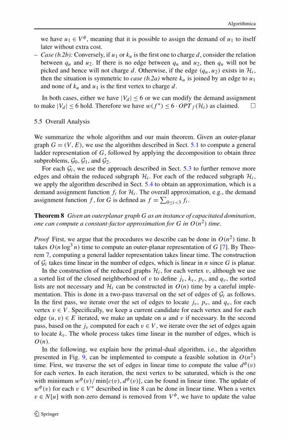
Algorithmica

we have u1 ∈ V φ , meaning that it is possible to assign the demand of u1 to itselflater without extra cost.

– Case (b.2b): Conversely, if u1 or ku is the first one to charge d , consider the relationbetween qu and u2. If there is no edge between qu and u2, then qu will not bepicked and hence will not charge d . Otherwise, if the edge (qu,u2) exists in Hi ,then the situation is symmetric to case (b.2a) where ku is joined by an edge to u1and none of ku and u1 is the first vertex to charge d .

In both cases, either we have |Vd | ≤ 6 or we can modify the demand assignmentto make |Vd | ≤ 6 hold. Therefore we have w(f ∗) ≤ 6 · OPTf (Hi ) as claimed. �

5.5 Overall Analysis

We summarize the whole algorithm and our main theorem. Given an outer-planargraph G = (V ,E), we use the algorithm described in Sect. 5.1 to compute a generalladder representation of G, followed by applying the decomposition to obtain threesubproblems, G0, G1, and G2.

For each Gi , we use the approach described in Sect. 5.3 to further remove moreedges and obtain the reduced subgraph Hi . For each of the reduced subgraph Hi ,we apply the algorithm described in Sect. 5.4 to obtain an approximation, which is ademand assignment function fi for Hi . The overall approximation, e.g., the demandassignment function f , for G is defined as f = ∑

0≤i<3 fi .

Theorem 8 Given an outerplanar graph G as an instance of capacitated domination,one can compute a constant-factor approximation for G in O(n2) time.

Proof First, we argue that the procedures we describe can be done in O(n2) time. Ittakes O(n log3 n) time to compute an outer-planar representation of G [7]. By Theo-rem 7, computing a general ladder representation takes linear time. The constructionof Gi takes time linear in the number of edges, which is linear in n since G is planar.

In the construction of the reduced graphs Hi , for each vertex v, although we usea sorted list of the closed neighborhood of v to define jv , kv , pv , and qv , the sortedlists are not necessary and Hi can be constructed in O(n) time by a careful imple-mentation. This is done in a two-pass traversal on the set of edges of Gi as follows.In the first pass, we iterate over the set of edges to locate jv , pv , and qv , for eachvertex v ∈ V . Specifically, we keep a current candidate for each vertex and for eachedge (u, v) ∈ E iterated, we make an update on u and v if necessary. In the secondpass, based on the jv computed for each v ∈ V , we iterate over the set of edges againto locate kv . The whole process takes time linear in the number of edges, which isO(n).

In the following, we explain how the primal-dual algorithm, i.e., the algorithmpresented in Fig. 9, can be implemented to compute a feasible solution in O(n2)

time. First, we traverse the set of edges in linear time to compute the value dφ(v)

for each vertex. In each iteration, the next vertex to be saturated, which is the onewith minimum wφ(v)/min{c(v), dφ(v)}, can be found in linear time. The update ofwφ(v) for each v ∈ V ∗ described in line 8 can be done in linear time. When a vertexv ∈ N [u] with non-zero demand is removed from V φ , we have to update the value

Algorithmica

dφ(v′) for all v′ ∈ N [v]. By Lemma 16, the closed degree of such vertices is boundedby 7. This update can be done in O(1) time. The construction of Su can be done inlinear time. Since dφ(v) can only decrease, each vertex can turn into lightly-loadedat most once. Therefore the overall processing time for these vertices is linear in thenumber of vertices. The outer-loop iterates at most O(n) times. Therefore the wholealgorithm runs in O(n2) time.

The feasibility of the demand assignment function f is guaranteed by Lemma 13and the fact that Hi is a subgraph of Gi . Since Hi ⊆ Gi , the demand assignment weobtained for Hi is also a feasible demand assignment for Gi . Therefore, f is feasiblefor G.

Putting everything together and we have

w(f ) ≤∑

0≤i<3

w(fi) Definition of f,

≤ 6 ·∑

0≤i<3

OPTf (Hi ) Lemma 18,

≤ 12 ·∑

0≤i<3

OPTf (Gi ) Lemma 16,

≤ 12 ·∑

0≤i<3

OPT(Gi ) ILP relaxation,

≤ 36 · OPT(G) Lemma 13. �

6 Planar Graphs

In this section, we show how the algorithms presented above can be extended toobtain approximation algorithms for planar graphs under a general framework dueto [3]. In Sect. 6.1 we sketch the framework and describe how the algorithms providedin Sect. 4.2 can lead to a pseudo-polynomial-time approximation scheme for planargraphs.

Regarding polynomial-time approximation algorithms, we prove in Sect. 6.2 thatapproximating this problem on planar graphs with inseparable demands to a factorsmaller than 3

2 − ε is weakly NP-hard, for any ε > 0. For the separable demandmodel, we show in Sect. 6.3 how the algorithm presented in Sect. 5 can be adoptedto obtain a constant-factor approximation for planar graphs.

6.1 The Framework

Let G = (V ,E) be a planar graph. We generate a planar embedding using the linear-time algorithm of Hopcroft and Tarjan [28]. To help present the framework, we definethe levels of the vertices with respect to this embeddings as follows. By level 1 wemean the set of vertices the lie on the unbounded face. For any j > 1, we refer levelj to as the set of vertices on the unbounded face after the removal of vertices in levels1,2, . . . , j − 1.

Algorithmica

Let m be the number of levels of this embedding, OPT be the cost of the optimaldemand assignment of G, and OPTj be the cost contributed by vertices at level j .For the ease of presentation, for any j with j ≤ 0 or j > m, the set of vertices in levelj is defined to be an empty set, and the corresponding cost OPTj is defined to bezero.

Let k ≥ 3 be a constant to be determined. For 0 ≤ i < k, we define Ci as

∑

0≤j≤ mk

(OPTk·j−i + OPTk·(j+1)−i−1).

Since∑

0≤i<k Ci ≤ 2 · OPT , there exists an i0 with 0 ≤ i0 < k such that Ci0 ≤ 2k

·OPT . For each 0 ≤ j ≤ m

k, define the graph Gj to be the graph induced by vertices

between level k · j − i0 and level k · (j + 1) − i0 − 1. The parameters of the verticesin Gj are set as follows. For those vertices which are from level k · j − i0 and levelk · (j + 1) − i0 − 1, their demands are set to be zero. The rest of the parametersremain unchanged. Clearly, Gj is a k-outerplanar graph, which has treewidth at most3k − 1 [3–5, 30], and we have

∑0≤j≤ m

kOPT(Gj ) ≤ (1 + 2

k) · OPT , where OPT(Gj )

is the cost of the optimal demand assignment of Gj .The following theorem follows directly from Theorem 6 in Sect. 4.2, Corollary 2

in Sect. 4.2, Lemma 5 in Sect. 3.3, and the decomposition described above.

Theorem 9 When the input graph is planar, one can compute the following approxi-mations for the capacitated domination problem in pseudo-polynomial time.

– (1+ 2k)-approximation in O(26k(logM+1)+log 3k ·n) time when the demand is insep-

arable, where M is the maximum capacity of the vertex set.– (1 + 2

k)-approximation in time O(2(2M+2N+1) log 3k · n) and

(2+ 2k)-approximation in time O(2(4M+1) log 3k ·n), when the demand is separable,

where M is the maximum capacity and N is the maximum demand of the vertexset.

Theorem 9 gives a parameterized approximation for both problem models in thesense that it allows a trade-off between the quality of the approximation results andthe running time of the algorithm.

6.2 A Lower Bound of ( 32 − ε) on the Approximation Factor for the Inseparable

Demand Model

Below we show that, when the demand is inseparable, it is weakly NP-hard to ap-proximate this problem within a factor of ( 3

2 − ε). The reduction is made from Par-tition, which is a well-known combinatorial problem that is known to be weaklyNP-hard [21].

Definition 9 (Partition problem) Given a sequence of positive integers a1, a2, . . . , an,the partition problem asks to decide whether or not there exists a subset A ⊆{1,2, . . . , n} such that

∑i∈A ai = ∑

1≤i≤n,i /∈A ai .

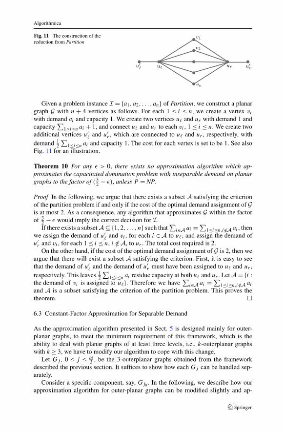
Algorithmica

Fig. 11 The construction of thereduction from Partition

Given a problem instance I = {a1, a2, . . . , an} of Partition, we construct a planargraph G with n + 4 vertices as follows. For each 1 ≤ i ≤ n, we create a vertex vi

with demand ai and capacity 1. We create two vertices u� and ur with demand 1 andcapacity

∑1≤i≤n ai + 1, and connect u� and ur to each vi , 1 ≤ i ≤ n. We create two

additional vertices u′� and u′

r , which are connected to u� and ur , respectively, withdemand 1

2

∑1≤i≤n ai and capacity 1. The cost for each vertex is set to be 1. See also

Fig. 11 for an illustration.

Theorem 10 For any ε > 0, there exists no approximation algorithm which ap-proximates the capacitated domination problem with inseparable demand on planargraphs to the factor of ( 3

2 − ε), unless P = NP.

Proof In the following, we argue that there exists a subset A satisfying the criterionof the partition problem if and only if the cost of the optimal demand assignment of Gis at most 2. As a consequence, any algorithm that approximates G within the factorof 3

2 − ε would imply the correct decision for I .If there exists a subset A ⊆ {1,2, . . . , n} such that

∑i∈A ai = ∑

1≤i≤n,i /∈A ai , thenwe assign the demand of u′

� and vi , for each i ∈ A to u�, and assign the demand ofu′

r and vi , for each 1 ≤ i ≤ n, i /∈A, to ur . The total cost required is 2.On the other hand, if the cost of the optimal demand assignment of G is 2, then we

argue that there will exist a subset A satisfying the criterion. First, it is easy to seethat the demand of u′

� and the demand of u′r must have been assigned to u� and ur ,

respectively. This leaves 12

∑1≤i≤n ai residue capacity at both u� and ur . Let A = {i :

the demand of vi is assigned to u�}. Therefore we have∑

i∈A ai = ∑1≤i≤n,i /∈A ai

and A is a subset satisfying the criterion of the partition problem. This proves thetheorem. �

6.3 Constant-Factor Approximation for Separable Demand

As the approximation algorithm presented in Sect. 5 is designed mainly for outer-planar graphs, to meet the minimum requirement of this framework, which is theability to deal with planar graphs of at least three levels, i.e., k-outerplanar graphswith k ≥ 3, we have to modify our algorithm to cope with this change.

Let Gj , 0 ≤ j ≤ m3 , be the 3-outerplanar graphs obtained from the framework

described the previous section. It suffices to show how each Gj can be handled sep-arately.

Consider a specific component, say, Gj0 . In the following, we describe how ourapproximation algorithm for outer-planar graphs can be modified slightly and ap-

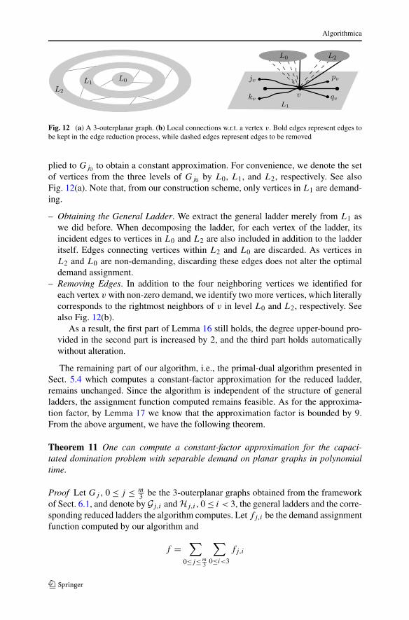
Algorithmica

Fig. 12 (a) A 3-outerplanar graph. (b) Local connections w.r.t. a vertex v. Bold edges represent edges tobe kept in the edge reduction process, while dashed edges represent edges to be removed

plied to Gj0 to obtain a constant approximation. For convenience, we denote the setof vertices from the three levels of Gj0 by L0, L1, and L2, respectively. See alsoFig. 12(a). Note that, from our construction scheme, only vertices in L1 are demand-ing.

– Obtaining the General Ladder. We extract the general ladder merely from L1 aswe did before. When decomposing the ladder, for each vertex of the ladder, itsincident edges to vertices in L0 and L2 are also included in addition to the ladderitself. Edges connecting vertices within L2 and L0 are discarded. As vertices inL2 and L0 are non-demanding, discarding these edges does not alter the optimaldemand assignment.

– Removing Edges. In addition to the four neighboring vertices we identified foreach vertex v with non-zero demand, we identify two more vertices, which literallycorresponds to the rightmost neighbors of v in level L0 and L2, respectively. Seealso Fig. 12(b).

As a result, the first part of Lemma 16 still holds, the degree upper-bound pro-vided in the second part is increased by 2, and the third part holds automaticallywithout alteration.

The remaining part of our algorithm, i.e., the primal-dual algorithm presented inSect. 5.4 which computes a constant-factor approximation for the reduced ladder,remains unchanged. Since the algorithm is independent of the structure of generalladders, the assignment function computed remains feasible. As for the approxima-tion factor, by Lemma 17 we know that the approximation factor is bounded by 9.From the above argument, we have the following theorem.

Theorem 11 One can compute a constant-factor approximation for the capaci-tated domination problem with separable demand on planar graphs in polynomialtime.

Proof Let Gj , 0 ≤ j ≤ m3 be the 3-outerplanar graphs obtained from the framework

of Sect. 6.1, and denote by Gj,i and Hj,i , 0 ≤ i < 3, the general ladders and the corre-sponding reduced ladders the algorithm computes. Let fj,i be the demand assignmentfunction computed by our algorithm and

f =∑

0≤j≤ m3

∑

0≤i<3

fj,i

Algorithmica

be the demand assignment function to the entire graph. We have

w(f ) ≤∑

0≤j≤ m3

∑

0≤i<3

w(fj,i) Definition of f,

≤ 9 ·∑

0≤j≤ m3

∑

0≤i<3

OPTf (Hj,i ) Lemma 17,

≤ 18 ·∑

0≤j≤ m3

∑

0≤i<3

OPTf (Gj,i ) Lemma 16,

≤ 18 ·∑

0≤j≤ m3

∑

0≤i<3

OPT(Gj,i ) ILP relaxation,

≤ 54 ·∑

0≤j≤ m3

OPT(Gj ) Lemma 13,

≤ 90 · OPT(G) Framework of Sect. 6.1.

This proves the theorem. �

Notice that, the framework used in this section does not depend on the separabil-ity of the demand. Hence any approximation for the inseparable demand model onk-outerplanar graphs for k ≥ 3 will imply an approximation for planar graphs as well.However, as our result for separable demand depends heavily on the linear programpresented in Sect. 5.2, at this moment we are not sure how corresponding approxima-tion results for inseparable demand model could be obtained.

7 Conclusion

In this paper, we studied a natural generalization of the dominating set under theconcept of capacitation, called capacitated domination, and provided approximationalgorithms as well as complexity results to compose a comprehensive study for thisproblem jointly with a series of previous work [31–33].

For general graphs, we provided logarithmic approximations which are asymptot-ically optimal. In terms of parameterized complexity, we showed that this problem isW[1]-hard with respect to the treewidth. For the positive side, we presented an FPTalgorithm which takes the treewidth and the maximum capacity of the vertices asparameters. The latter implies a pseudo-polynomial time approximation scheme forplanar graphs.

To drop the pseudo-polynomial factor of the approximation, we developed aconstant-factor approximation for outerplanar graphs with separable demands fol-lowed by augmenting the algorithm to obtain a constant-factor approximation forplanar graphs with separable demands. For planar graphs with inseparable demands,we showed that, unless P = NP , the approximation factor of any algorithm is at least32 − ε, for any ε > 0.

Below, we conclude by listing related open problems. First, due to the flexibil-ity of the ways the demand can be assigned, the approximation result we provided

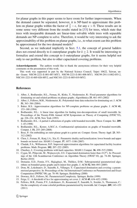
Algorithmica

for planar graphs in this paper seems to have room for further improvements. Whenthe demand cannot be separated, however, it is NP-hard to approximate this prob-lem on planar graphs within the factor of 3

2 − ε, for any ε > 0. These results are insome sense very different from the results stated in [33] for trees, which state thattrees with inseparable demands are linear-time solvable while trees with separabledemands are NP-complete to solve. Therefore, it would be very interesting to ask theapproximability of this problem on planar graphs, i.e., to what extent can this problembe approximated for the two demand models?

Second, as we indicated implicitly in Sect. 5.1, the concept of general laddersdoes not extend directly to k-outerplanar graphs for k ≥ 2. It would be interesting toformalize and extend this concept to k-outerplanar graphs, for it seems helpful notonly to our problem, but also to other capacitated covering problems.

Acknowledgements The authors would like to thank the anonymous referees for their very helpfulcomments on the presentation of this work.

This work was supported in part by the National Science Council, Taipei 10622, Taiwan, un-der Grants NSC98-2221-E-001-007-MY3, NSC98-2221-E-001-008-MY3, NSC99-2911-I-002-055-2,NSC101-2221-E-005-026-MY2, and NSC101-2221-E-005-019-MY2.

References

1. Alber, J., Bodlaender, H.L., Fernau, H., Kloks, T., Niedermeier, R.: Fixed parameter algorithms fordominating set and related problems on planar graphs. Algorithmica 33, 461–493 (2002)

2. Alber, J., Fellows, M.R., Niedermeier, R.: Polynomial-time data reduction for dominating set. J. ACM51, 363–384 (2004)

3. Baker, B.S.: Approximation algorithms for NP-complete problems on planar graphs. J. ACM 41,153–180 (1994)

4. Bodlaender, H.L.: A linear time algorithm for finding tree-decompositions of small treewidth. In:Proceedings of the Twenty-Fifth Annual ACM Symposium on Theory of Computing (STOC’93),pp. 226–234. ACM, New York (1993)

5. Bodlaender, H.L.: A partial k-arboretum of graphs with bounded treewidth. Theor. Comput. Sci. 209,1–45 (1998)

6. Bodlaender, H.L., Koster, A.M.C.A.: Combinatorial optimization on graphs of bounded treewidth.Comput. J. 51, 255–269 (2008)

7. Bose, P.: On embedding an outer-planar graph in a point set. Comput. Geom. Theory Appl. 23, 303–312 (2002)

8. Chen, J., Fernau, H., Kanj, I.A., Xia, G.: Parametric duality and kernelization: lower bounds and upperbounds on kernel size. SIAM J. Comput. 37, 1077–1106 (2007)

9. Chudak, F.A., Williamson, D.P.: Improved approximation algorithms for capacitated facility locationproblems. Math. Program. 102, 207–222 (2005)

10. Chuzhoy, J.: Covering problems with hard capacities. SIAM J. Comput. 36, 498–515 (2006)11. Cygan, M., Pilipczuk, M., Wojtaszczyk, J.O.: Capacitated domination faster than O(2n). In: Proceed-

ings of the 12th Scandinavian Conference on Algorithm Theory (SWAT’10), pp. 74–80. Springer,Berlin (2010)

12. Demaine, E.D., Fomin, F.V., Hajiaghayi, M., Thilikos, D.M.: Subexponential parameterized algo-rithms on bounded-genus graphs and h-minor-free graphs. J. ACM 52, 866–893 (2005)

13. Dom, M., Lokshtanov, D., Saurabh, S., Villanger, Y.: Capacitated domination and covering: a param-eterized perspective. In: Proceedings of the 3rd International Conference on Parameterized and ExactComputation (IWPEC’08), pp. 78–90. Springer, Heidelberg (2008)

14. Downey, R.G., Fellows, M.: Parameterized Complexity. Springer, Berlin (1999)15. Feige, U.: A threshold of lnn for approximating set cover. J. ACM 45, 634–652 (1998)16. Fellows, M.R., Fomin, F.V., Lokshtanov, D., Rosamond, F., Saurabh, S., Szeider, S., Thomassen, C.:

On the complexity of some colorful problems parameterized by treewidth. Inf. Comput. 209, 143–153(2011)

Algorithmica

17. Flum, J., Grohe, M.: Parameterized Complexity Theory. Springer, Berlin (2006)18. Fomin, F.V., Thilikos, D.M.: Dominating sets in planar graphs: branch-width and exponential speed-

up. SIAM J. Comput. 36, 281–309 (2006)19. Gandhi, R., Halperin, E., Khuller, S., Kortsarz, G., Srinivasan, A.: An improved approximation algo-

rithm for vertex cover with hard capacities. J. Comput. Syst. Sci. 72, 16–33 (2006)20. Gandhi, R., Khuller, S., Parthasarathy, S., Srinivasan, A.: Dependent rounding in bipartite graphs. In:

Proceedings of the 43rd Symposium on Foundations of Computer Science (FOCS’02), pp. 323–332.IEEE Comput. Soc., Washington (2002)

21. Garey, M.R., Johnson, D.S.: Computers and Intractability: A Guide to the Theory of NP-Complete-ness. Freeman, New York (1979)

22. Guha, S., Hassin, R., Khuller, S., Or, E.: Capacitated vertex covering. J. Algorithms 48, 257–270(2003)

23. Guo, J., Niedermeier, R.: Linear problem kernels for NP-hard problems on planar graphs. In: Proceed-ings of the 34th International Conference on Automata, Languages and Programming (ICALP’07),pp. 375–386. Springer, Berlin (2007)

24. Hagerup, T.: Simpler linear-time kernelization for planar dominating set. In: Proceedings of the 6thInternational Conference on Parameterized and Exact Computation (IPEC’11), pp. 181–193. Springer,Berlin (2012)

25. Haynes, T.W., Hedetniemi, S., Slater, P.: Fundamentals of Domination in Graphs (Pure and AppliedMathematics). Dekker, New York (1998)

26. Haynes, T.W., Hedetniemi, S.M., Hedetniemi, S.T., Henning, M.A.: Domination in graphs applied toelectric power networks. SIAM J. Discrete Math. 15, 519–529 (2002)

27. Hochbaum, D.S.: Approximation algorithms for the set covering and vertex cover problems. SIAM J.Comput. 11, 555–556 (1982)

28. Hopcroft, J., Tarjan, R.: Efficient planarity testing. J. ACM 21, 549–568 (1974)29. Johnson, D.S.: Approximation algorithms for combinatorial problems. J. Comput. Syst. Sci. 9, 256–

278 (1974)30. Kammer, F., Tholey, T.: Approximate tree decompositions of planar graphs in linear time. In: Pro-

ceedings of the Twenty-Third Annual ACM-SIAM Symposium on Discrete Algorithms (SODA’12),pp. 683–698. SIAM, Philadelphia (2012)

31. Kao, M.-J., Chen, H.-L.: Approximation algorithms for the capacitated domination problem. In: FAW2010, pp. 185–196. Springer, Berlin (2010)

32. Kao, M.-J., Lee, D.T.: Capacitated domination: constant factor approximations for planar graphs.In: Proceedings of the 22nd International Conference on Algorithms and Computation (ISAAC’11),pp. 494–503. Springer, Berlin (2011)

33. Kao, M.-J., Liao, C.-S., Lee, D.T.: Capacitated domination problem. Algorithmica 60, 274–300(2011)

34. Kloks, T.: Treewidth, Computations and Approximations. Lecture Notes in Computer Science,vol. 842. Springer, Berlin (1994)

35. Liao, C.-S., Lee, D.-T.: Power domination problem in graphs. In: Proceedings of the 11th AnnualInternational Conference on Computing and Combinatorics (COCOON’05), pp. 818–828. Springer,Berlin (2005)

36. Liedloff, M., Todinca, I., Villanger, Y.: Solving capacitated dominating set by using covering bysubsets and maximum matching. Discrete Appl. Math. (2012)

37. Niedermeier, R.: Invitation to Fixed Parameter Algorithms. Oxford University Press, Oxford (2006)38. Pál, M., Tardos, E., Wexler, T.: Facility location with nonuniform hard capacities. In: Proceedings of

the 42nd IEEE Symposium on Foundations of Computer Science (FOCS’01), p. 329. IEEE Comput.Soc., Washington (2001)

39. Roberts, F.S.: Graph Theory and Its Applications to Problems of Society (1978)40. Shmoys, D.B., Tardos, E., Aardal, K.: Approximation algorithms for facility location problems (ex-

tended abstract). In: STOC 1997, pp. 265–274. ACM, New York (1997)41. van Bevern, R., Hartung, S., Kammer, F., Niedermeier, R., Weller, M.: Linear-time computation of

a linear problem kernel for dominating set on planar graphs. In: Proceedings of the 6th Interna-tional Conference on Parameterized and Exact Computation (IPEC’11), pp. 194–206. Springer, Berlin(2012)

42. Vazirani, V.V.: Approximation Algorithms. Springer, New York (2001)43. Wan, P.-J., Alzoubi, K.M., Frieder, O.: A simple heuristic for minimum connected dominating set in

graphs. Int. J. Found. Comput. Sci. 14, 323–333 (2003)