Capital structure: profitability, earnings volatility and

Capital structure: profitability, earnings volatility

and the probability of financial distress

Jacque Dreyer

Student Number: 28530366

A research project submitted to the Gordon Institute of Business Science, University

of Pretoria, in partial fulfilment of the requirements for the degree of Master of

Business Administration.

November 2010

© 2010 University of Pretoria. All rights reserved. The copyright in this work vests in the University of Pretoria. No part of this work may be reproduced or transmitted in any form or by any means, without the prior written permission of the University of Pretoria.

©© UUnniivveerrssiittyy ooff PPrreettoorriiaa

Abstract This research project set out to determine whether there is a relationship between

the observed leverage levels of South African companies, their profitability, earnings

volatility and the probability of financial distress. The relevant body of knowledge

against which to execute this research project is known as capital structure theory.

Capital structure theory deals with the way in which firms finance themselves. It is

concerned with the relationship between the structure of debt, equity and hybrid

securities found on the right hand side of the firm’s balance sheet.

It is believed that the 2007/8 global financial crisis offers researchers a unique

opportunity to gain insight into how the observed leverage levels of firms and their

earnings volatility interact to form their probability of financial distress. This area of

research is of particular interest since it is commonly believed and frequently stated

that South African firms are underleveraged and secondly because there is contrarian

research beginning to be published indicating that firms with very little or no debt

(commonly referred to as lazy balance sheets) are outperforming their more

indebted peers and are being rewarded by investors for their prudence.

Keywords: Capital structure; Leverage; Financial distress; pecking order

ii


Declaration I declare that this research project is my own work. It is submitted in partial

fulfilment of the requirements for the degree of Master of Business Administration at

the Gordon Institute of Business Science, University of Pretoria. It has not been

submitted before for any degree or examination in any other University. I further

declare that I have obtained the necessary authorisation and consent to carry out this

research.

___________________________

Jacque Dreyer

November 2010

iii


Acknowledgements As with most things in life the process of completing this dissertation and the MBA

program in general has required the input, cooperation and support of many people.

I would like to specifically thank the following people:

Firstly my wife, Natascha, thank you for your support, patience and encouragement. I

know that this journey required you to make many sacrifices for which I am thankful.

To my research supervisors, Zenobia Ismael and Kuber Thaver, thank you for your

support and guidance. Having a research student that changes his topic and direction

mid‐course is never something easy to do but you have weathered the storm

wonderfully.

To Rudy Rudolph at Endress+Hauser, thank you for allowing me the opportunity to do

this MBA. I know that this was not the accepted norm at our small South African

subsidiary and my absence and distraction has placed a lot of strain on everybody

around me.

To my friends, I am looking forward to regaining a social dimension to my life again.

iv


Table of Contents

Abstract................................................................................................................................................... ii

Keywords:................................................................................................................................................ ii

Declaration............................................................................................................................................. iii

Acknowledgements................................................................................................................................ iv

Table of figures .................................................................................................................................... viii

List of tables........................................................................................................................................... ix

1. Chapter One – Introduction .........................................................................................................11

1.1. Research title ........................................................................................................................11

1.2. Research problem ................................................................................................................11

1.3. Research aim ........................................................................................................................16

2. Chapter two – Literature review..................................................................................................19

2.1. Introduction..........................................................................................................................19

2.2. Maximising shareholder wealth ..........................................................................................20

2.3. Defining capital structure research .....................................................................................21

2.4. Capital structure theories ....................................................................................................23

2.4.1. Capital structure irrelevance.........................................................................................23

2.4.2. Trade‐off theory............................................................................................................25

2.4.2.1. The advantages of debt.............................................................................................28

2.4.2.2. The cost of debt ........................................................................................................29

2.4.3. Pecking order theory.....................................................................................................32

2.4.4. The market timing theory of capital structure .............................................................34

2.5. Financial distress ..................................................................................................................35

2.7. Conclusion ............................................................................................................................40

3. Chapter Three – Research questions and hypothesis .................................................................42

3.1. Research hypothesis one: the relationship between profitability and debt .....................42

3.2. Research hypothesis two: difference between industry median debt levels ....................43

3.3. Research hypothesis three: the relationship between earnings volatility and debt.........44

3.4. Research hypothesis four: the relationship between the price‐to‐book ratio and debt 45

3.5. Research hypothesis five: the relationship between debt and the probability of financial

distress..............................................................................................................................................45

4. Chapter four ‐ Research Methodology ........................................................................................47

4.1. Introduction..........................................................................................................................47

4.2. Population of relevance .......................................................................................................47

v


4.3. Unit of analysis .....................................................................................................................48

4.4. Sampling Method .................................................................................................................48

4.5. Data collection process ........................................................................................................48

4.6. Data analysis process ...........................................................................................................49

4.6.1. Descriptive statistics .....................................................................................................49

4.6.2. Exploring the relationships between variables.............................................................51

4.6.3. Defining the dependant variables.................................................................................55

4.6.4. Cross sectional, longitudinal and panel data ................................................................55

4.6.5. Financial ratios ..............................................................................................................57

4.6.6. Hypothesis testing.........................................................................................................59

4.7. Research limitations .............................................................................................................60

4.8. Conclusion ............................................................................................................................61

5. Chapter Five – Presentation of Results .......................................................................................62

5.1. Introduction..........................................................................................................................62

5.2. General information and descriptive statistics for the sample data..................................62

5.3. Research hypothesis one: the relationship between profitability and debt .....................66

5.3.1. Leverage and ROA ........................................................................................................66

5.3.2. Industry median debt levels..........................................................................................71

5.3.3. Leverage and earnings volatility ...................................................................................74

5.3.4. Leverage and the price‐to‐book ratio ...........................................................................77

5.3.5. D/E and default probability...........................................................................................81

6.2. Discussion of results .............................................................................................................88

6.2.1. Research hypothesis one: the relationship between profitability and debt ................88

6.2.2. Research hypothesis two: difference between industry median debt levels...............90

6.2.3. Research hypothesis three: the relationship between earnings volatility and debt....91

6.2.4. Research hypothesis four: the relationship between the price‐to‐book ratio and

debt 92

6.2.5. Research hypothesis five: the relationship between debt and the probability of

financial distress ...........................................................................................................................93

7. Chapter seven – Conclusion and recommendations...................................................................96

7.1. Introduction..........................................................................................................................96

7.2. Summary of key findings......................................................................................................96

7.3. Recommendations ...............................................................................................................99

7.3.1. Recommendations for practitioners................................................................................99

vi


7.3.2. Recommendations for researchers................................................................................100

7.4. Suggestions for further research .......................................................................................100

7.5. Conclusion ..........................................................................................................................102

8. References ..................................................................................................................................104

vii


Table of figures

Figure 1: Application and sources of funding (Adapted from Ward & Price, 2006 pgs. 24‐25)..22

Figure 2: Abbreviated balance sheet (Myers, 2002 pg. 5) ..........................................................24

Figure 3: Capital cost and the optimal capital structure (Gitman, 2003, p.544) ........................27

Figure 4: Conceptual overview of capital structure landscape (adapted from Rayan, 2008).....38

Figure 5: Number of firms per sector included in the research project .....................................63

Figure 6: D/E Histogram for all industries included in the sample .............................................64

Figure 7: D/E Box plot for all industries included in the sample.................................................64

Figure 8: Box plot for the comparison of means of D/E vs. ROA ................................................67

Figure 9: Normal probability plot for D/E and ROA ....................................................................67

Figure 10: Correlation between D/E and ROA ............................................................................70

Figure 11: Box plot for the industry mean debt levels................................................................72

Figure 12: Box plot for the D/E ratio of firms based on their earnings volatility........................74

Figure 13: Normal probability plot for D/E versus earnings volatility ........................................75

Figure 14: Box plots for D/E versus the price‐to‐book‐ratio .......................................................78

Figure 15: Normal probability plots for D/E versus the price‐to‐book‐ratio ..............................78

Figure 16: Test of assumptions section for D/E versus the price‐to‐book‐ratio.........................79

Figure 17: Hypothesis test for D/E versus the price‐to‐book‐ratio.............................................79

Figure 18: Scatter diagram for D/E versus the price‐to‐book‐ratio ............................................80

Figure 19: Descriptive statistics for D/E versus financial distress probability............................81

Figure 20: Financial distress scores box plot...............................................................................81

Figure 21: The normal probability plot for the financial distress scores ....................................82

Figure 22: Box plots for financial distress versus interest coverage...........................................86

Figure 23: Normal probability plots for financial distress versus interest coverage ..................86

viii


List of tables

Table 1: Leverage in relation to explanatory variable under different capital structure theories

(based on data extracted from Frank & Goyal, 2009).................................................................17

Table 2: Selection matrix for the appropriate test for differences between the mean values of

two groups ..................................................................................................................................52

Table 3: Choosing an appropriate parametric or non‐parametric test (Cameron and Price,

2009 pg. 484)............................................................................................................................... 54

Table 4: Example of panel data with time series and cross Sectional data highlighted .............57

Table 5: Descriptive statistics for D/E and ROA ..........................................................................66

Table 6: Test of assumptions of normality for D/E and ROA ......................................................68

Table 7: Test for the differences between means for D/E versus ROA.......................................68

Table 8: Industry median debt levels test for normality.............................................................73

Table 9: Descriptive statistics for D/E and earnings volatility.....................................................74

Table 10: Test of assumptions section for D/E versus earnings volatility...................................75

Table 11 : Test for the differences between means for D/E versus earnings volatility ..............76

Table 12: Descriptive statistics for D/E versus the price‐to‐book‐ratio ......................................77

Table 13: Test of assumptions for the financial distress scores..................................................83

Table 14: Hypothesis test section for D/E versus financial distress probability .........................83

Table 15: Descriptive statistics for financial distress versus interest coverage..........................85

Table 16: Test of assumptions section for financial distress versus interest coverage ..............87

Table 17: Hypothesis test for financial distress versus interest coverage ..................................87

ix


List of equations

Equation 1: Value of the firm under perfect market conditions (Firer et al, 2008, pg 524) .......24

Equation 2: Value of the levered firm (Firer et al, 2008 pg. 524) ...............................................25

Equation 3: Sample mean (Albright et al, 2006 pg. 82) ..............................................................49

Equation 4: The relationship between standard deviation and variance (Albright et al, 2006

pg. 87)..........................................................................................................................................50

Equation 5: ROA (Firer et al, 2008 pg. 65)...................................................................................57

Equation 7: Debt‐to‐equity ratio (Firer et al, 2008 pg. 60) .........................................................58

Equation 8: Altman Z score (Bodie, Kane & Marcus, 2009 pg. 470) ...........................................58

x


11

1. Chapter One – Introduction

1.1. Research title

Capital structure: profitability, earnings volatility and the probability of financial

distress.

1.2. Research problem

Since the introduction of the Miller and Modigliani capital structure irrelevance

theorem the existence and determination of an optimal capital structure have been

one of the most controversial issues in corporate finance (Ryen, Vasconcellos & Kish,

1997). Despite the fact that there is a substantiate body of research about capital

structure theory academics are still not able to utilise the existing theory to explain

capital structure choice in practise or give practitioners guidance with regard to the

optimal mix between debt and equity in their financing decisions (Cai & Gosh, 2003).

According to Myers (2001) there is no unifying theory on the choice between debt

and equity and no reason to expect one either, there are however several theories

that are “conditionally useful” for explaining capital structure choice. This view is

supported by Frydenburg (2004) who states that current research does not point to a

single capital structure theory that adequately explains capital structure choice.

Harris and Raviv (1991) state that the various models and theories they have

surveyed identified a large number of potential determinants of capital structure but

that the empirical work does not point out which of these factors are (reliably)

important in various contexts. Some of these contexts include the increases and

decreases in profitability, increases and decreases in free cash flow, changes in


liquidation values of the firm, probability of financial distress and changes in the price

of the firms common stock to name but a few. Although they specifically exclude tax

based theories (stating that this is not their comparative research strength) Harris

and Raviv (1991) categorise the non‐tax based categories of capital structure into

four broad groups, namely:

I. Conflict of interest based approaches (i.e. agency cost)

II. Conveyance of information based approaches (i.e. asymmetric information)

III. Factors that influence the nature of competition or products (i.e. input/output

based approaches)

IV. Factors that will influence the outcome of corporate control contest

Norton (1991) indicated that one potential reason for the lack of agreement in capital

structure theory may be the fact that factors affecting capital structure choices are

not easily and objectively quantified by outside researchers. Norton states that these

factors include information asymmetries between managers and the marketplace,

expected bankruptcy cost, managerial risk preferences and the agency cost of

monitoring management. Titman and Wessels (1988) corroborate this view stating

that there are serious shortcomings in empirical tests of capital structure including:

I. There may be no unique representation for the attributes researchers wish to

measure. There are often several possible proxies for any particular attribute and

researchers lacking theoretical guidelines, may be tempted to select those variables

that work best in terms of statistical goodness‐of‐fit criteria thereby biasing the

significance levels of their tests

12


II. It is often difficult to find measures of particular attributes that are unrelated to

other attributes of interest, thus the selected proxy variables may be measuring the

effect of several different attributes

III. Since the observed variables are imperfect representations of the attributes they

are supposed to measure their use in regression analysis introduces an errors‐in‐

variable problem

IV. Measurement errors in the proxy variables may be correlated with measurement

error in the dependant variables creating spurious correlations even when the

unobserved attribute being measured is unrelated to the dependant variable

Harris and Raviv (2007, 2009) do however point to six core factors that have been

shown to be primarily responsible for the observed leverage levels:

a) Industry median leverage – firms that operate in industries that have high levels of

leverage tend to have high levels of leverage

b) Asset tangibility – leverage is positively correlated with asset tangibility

c) Profits – profitability and leverage is negatively correlated

d) Firm size – firm size and leverage is positively correlated

e) The market‐to‐book value of assets – market‐to‐book value of assets and leverage

are negatively correlated

13


f) Expected inflation – in high inflationary environments firms tend to increase their

leverage

Two of the most popular theories used to explain capital structure choice, and the

departure point for this study, are the trade‐off theory and the pecking order theory.

The trade‐off theory states that firms will pursue the tax deductibility of debt

weighted against the potential financial distress associated with excessive leverage in

their capital structures. The level of leverage a firm has in its capital structure is

therefore a balancing act between the benefits and cost of debt. The trade‐off theory

suggests that there is an optimal ratio between debt and equity (Myers 2001).

The pecking order theory proposes a hierarchy of funding preferences by managers

starting with internal sources of funds (i.e. retained earnings) followed by external

sources of funds, namely debt and equity, in order of preference. The pecking order

does not suggest an optimal ratio between debt and equity (Myers, 1984).

According to Fama and French (2005) both the trade‐off model and pecking order

model have serious shortcomings that prevent them from explaining capital structure

and therefore it does not make sense to continue to run empirical tests in an attempt

to see which theory best describes market behaviour, rather the two theories should

be seen as complimentary to each other in being able to describe some aspect of

financing decisions.

In contrast to the trade‐off and pecking order theories of capital structure Baker and

Wurgler (2002) observed that companies with low leverage levels tended to raise

funds when their share valuations were high and those with high leverage tended to

14


raise funds when their share valuations were low. They claim that these results

cannot be explained within the traditional theories of capital structure hence they

propose a market timing theory of capital structure which seems to offer substantial

explanatory power over chosen capital structures. The market timing theory is

disputed by DeAngelo, DeAngelo and Stulz (2010) who argue that firms near term

funding needs are a more reliable indication of equity issues and that market timing

is subordinated to capital requirements not a cause of it.

According to Frank and Goyal (1993) one of the reasons why no conclusive answers

to capital structure questions can be given, despite vast amounts of theoretical

literature and hundreds of empirical tests, is that many empirical studies are aimed at

giving support for a particular theory. Although this might be adequate for a given

paper it does not benefit our understanding of capital structure decisions. Several

researchers (Pinegar & Wilbricht, 1989; Brounen, de Jong & Koedijk, 2004) have

attempted to bridge the gap though survey research in order to try and explain how

managers make decisions with regard to capital structure. According to Pinegar and

Wilbricht (1989) their results indicate that financial planning principles are more

important in governing the financing decision of the firm than are specific capital

structure theories. This view is supported by Graham and Harvey (2002) who found

that although financial theory is incorporated into capital budgeting decisions

through the use of principles like Net Present Value (NPV) and Discounted Cash Flow

(DCF) calculations, finance professionals are not likely to pay attention to capital

structure theory but rather rely on practical, informal rules of thumb.

15


1.3. Research aim

According to Titman and Wessels (1988) a substantiate amount of empirical research

has been done on the determinants of the observed capital structure of firms. In

most cases this is done by identifying a number of potential explanatory variables and

regressing the explanatory variables against the firm’s capital structure. The most

common variables that have been used as explanatory (independent) variables

include profitability, asset tangibility, earnings volatility, non‐debt tax shields and

growth opportunities.

The aim of this research is to test three of these capital structure determinants

against the observed leverage witnessed in firms over the 1998‐2007 periods. The

explanatory variables that will be tested in the South African context are:

a) Profitability

b) Earnings volatility

c) Industry median leverage and the observed leverage of the firm

The predictions of the trade‐off and pecking order theories are outlined in the table

on the following page:

16


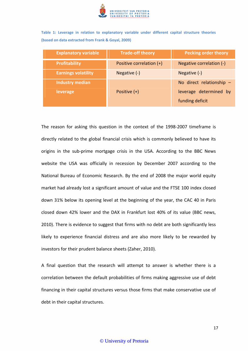
Table 1: Leverage in relation to explanatory variable under different capital structure theories

(based on data extracted from Frank & Goyal, 2009)

Explanatory variable Trade‐off theory Pecking order theory

Profitability Positive correlation (+) Negative correlation (‐)

Earnings volatility Negative (‐) Negative (‐)

Industry median

leverage

Positive (+)

No direct relationship –

leverage determined by

funding deficit

The reason for asking this question in the context of the 1998‐2007 timeframe is

directly related to the global financial crisis which is commonly believed to have its

origins in the sub‐prime mortgage crisis in the USA. According to the BBC News

website the USA was officially in recession by December 2007 according to the

National Bureau of Economic Research. By the end of 2008 the major world equity

market had already lost a significant amount of value and the FTSE 100 index closed

down 31% below its opening level at the beginning of the year, the CAC 40 in Paris

closed down 42% lower and the DAX in Frankfurt lost 40% of its value (BBC news,

2010). There is evidence to suggest that firms with no debt are both significantly less

likely to experience financial distress and are also more likely to be rewarded by

investors for their prudent balance sheets (Zaher, 2010).

A final question that the research will attempt to answer is whether there is a

correlation between the default probabilities of firms making aggressive use of debt

financing in their capital structures versus those firms that make conservative use of

debt in their capital structures.

17


In answering these research questions this research project aims to give additional

insight into the capital structure decisions of South African firms. A distinguishing

factor of this research project is the fact that this research incorporates the impact of

an external financial and economic shock (the global financial crisis) in an effort to

determine what impact such an externality had on firms with varying levels of

leverage. In answering this question the research hopes to be able to give a unique

and contrarian insight into the commonly held notion that South African firms are

under leveraged (Firer, Ross, Westerfield & Jordan, 2008).

18


2. Chapter two – Literature review

2.1. Introduction

Capital structure decisions can have important implications for the value of the firm

and its cost of capital (Firer et al, 2008 pg. 507). Poor capital structure decisions can

lead to an increased cost of capital thereby lowering the net present value (NPV) of

many of the firm’s investment projects to the point of making many investment

projects unacceptable (known as the underinvestment problem). Effective capital

structure decisions will lower the firms overall cost of capital and raise the NPV of

investment projects leading to more projects being acceptable to undertake and

consequently increasing the overall value of the firm (Gitman, 2003).

Despite the importance that capital structure can play in adding value to the firm

decades worth of theoretical literature and empirical testing have not been able to

give guidance to practitioners with regards to the choice between debt and equity in

their capital structures (Frank and Goyal, 2009). What is perplexing for anyone trying

to make sense of the capital structure literature is the fact that the different capital

structure theories are often diametrically opposed in their predictions while at other

times they may be in agreement but have different views about why the outcome has

been predicted. For this reason Myers (2002) stated that there is no universal theory

of capital structure, only conditional ones. Factors that are important in one context

may prove unimportant in another.

Perhaps it is for this reason that Barclay and Smith (2010) states that much of finance

education was designed to pass on to finance students rules of thumb derived from

the actions of successful practitioners. For this reason it has become of growing

19


importance to “develop theory to yield more precise predictions, and to devise more

powerful empirical tests as well as better proxies for the key firm characteristics that

are likely to drive corporate financing decisions” (Barclay & Smith, 2010 pg. 9).

2.2. Maximising shareholder wealth

The commonly stated goal of financial management is to maximise the wealth of the

owners or shareholders of the firm. Shareholder wealth in turn is defined as the

current price of the firm’s outstanding ordinary shares. It should be emphasised that

shareholders only have a residual claim to the assets of the firm and therefore they

will only be paid after every other stakeholder with a legal claim has been paid.

Because debt holders, suppliers of goods and services and employees all have a

priority claim it stands to reason that if the wealth of the shareholders are maximised

all other parties will stand to benefit (or at least not be disadvantaged) if this goal is

fulfilled. It should however be noted that profit maximisation and wealth

maximisation are not synonymous. A firm can undertake a variety of actions that

might improve short term profit that are either not translated into cash flows (i.e.

selling to firms or individuals that have no realistic probability of paying) or engaging

in other practises that are either not sustainable or ethical. The timing and magnitude

of cash flows and their associated risk are therefore the key drivers of the firms share

price and the wealth maximisation of the owners of the firm (Gitman, 2003; Firer et

al, 2008).

20


In achieving the goal of shareholder wealth maximisation managers are faced with

two important financial decisions, the investment decision and the financing decision.

Investment decisions or capital budgeting decisions refer to decisions about whether

to finance a project or assets and ensuring that the cash flows received from a project

or asset exceeds the cost incurred in acquiring that asset or implementing the

project. The financing decision refers to the way in which the asset or project are

financed. Financial managers therefore have to decide whether they will fund the

assets and projects of the firm through retained earnings, borrowings or equity or a

combination of the aforementioned options. The mixture chosen will affect both the

firms cost of capital, its risk and associated return and hence the value of its shares

(Gitman, 2003; Correia & Cramer, 2008).

2.3. Defining capital structure research

The study of capital structure focuses on the mix between debt, equity and the

variety of hybrid instruments used to finance the real investment of the firm. It is

therefore concerned with the right hand side of the balance sheet (Myers, 2001). All

the items on the right hand side of the balance sheet, excluding current liabilities, are

sources of capital employed to finance the real assets required to conduct the

business of the firm. Graphically a simplified capital the capital structure can be

illustrated as:

21


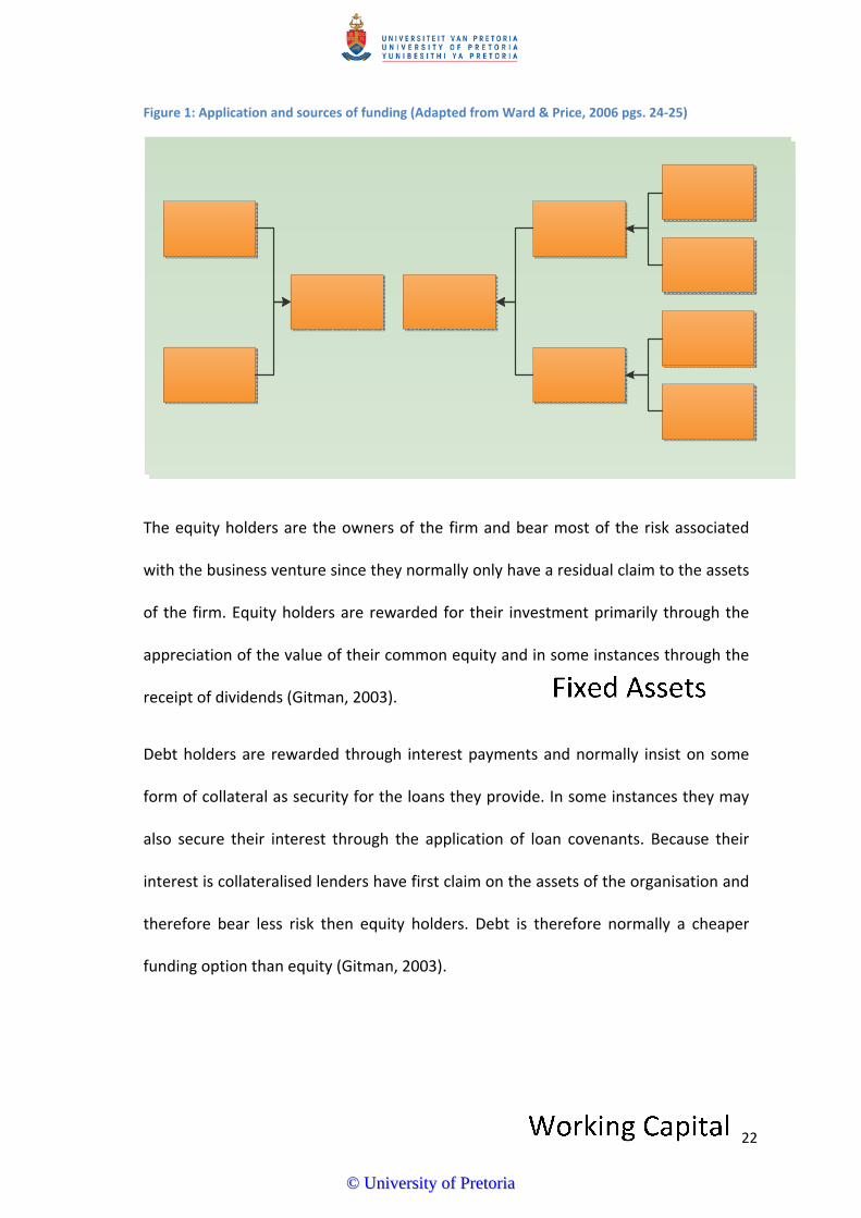
Figure 1: Application and sources of funding (Adapted from Ward & Price, 2006 pgs. 24‐25)

The equity holders are the owners of the firm and bear most of the risk associated

with the business venture since they normally only have a residual claim to the assets

of the firm. Equity holders are rewarded for their investment primarily through the

appreciation of the value of their common equity and in some instances through the

receipt of dividends (Gitman, 2003).

Debt holders are rewarded through interest payments and normally insist on some

form of collateral as security for the loans they provide. In some instances they may

also secure their interest through the application of loan covenants. Because their

interest is collateralised lenders have first claim on the assets of the organisation and

therefore bear less risk then equity holders. Debt is therefore normally a cheaper

funding option than equity (Gitman, 2003).

22


According to Ward and Price (2006) if you want to evaluate the performance of the

firm it is important to consider all interest bearing borrowings as loan capital

regardless of whether they are short term or long term loans.

Companies manage their capital structure through the issuance of new debt and

equity, by repaying debt or repurchasing shares. Other aspects relating to

management of the capital structure such as risk management, the issuance of hybrid

securities and various classes of bonds, dividend pay‐out management etc. fall largely

beyond the scope of this research.

2.4. Capital structure theories

Although there are numerous capital structure theories only the three most

pervasive capital structure theories, the trade‐off theory, the pecking order theory

and the market timing theory will be reviewed for the purposes of this study.

2.4.1. Capital structure irrelevance

The departure point for virtually all discussions on capital structure theory is

Modigliani and Miller’s capital structure irrelevance theory first published in 1958.

According to the theory the way in which a firm finances its assets (through the mix

of debt and equity) can have no impact on the value of the firm. The value of a firm is

derived by the productivity and the quality of the assets in which the firm has

invested. Consider the following abbreviated balance sheet:

23


Figure 2: Abbreviated balance sheet (Myers, 2002 pg. 5)

Considering the right hand side of the balance sheet the value of the firm (V) will

remain the same regardless of how the ratio between debt and equity is varied

(Myers, 2001). It is therefore possible to state:

Equation 1: Value of the firm under perfect market conditions (Firer et al, 2008, pg. 524)

Where:

VL = the value of a levered firm

VU = the value of an unlevered firm

It is important to note however that the Modigliani and Miller capital structure

irrelevance theory only holds under the assumption of perfect capital markets which

were defined by Modigliani and Miller (1958) as:

a) The shares of different firms are homogenous and are therefore perfect substitutes

for one another

b) All shares are traded under perfect market conditions

c) Investors are in agreement about the expected future returns for all shares

d) The cost of debt is the same regardless of the issuer of the debt

24


Modigliani and Miller (1958) conclude their seminal paper by remarking that these

restrictive assumptions were necessary to come to grips with the capital structure

problem, “Having served their purpose they can now be relaxed in the direction of

greater realism and relevance” (Modigliani and Miller, 1958 pg. 296).

2.4.2. Trade‐off theory

Modigliani and Miller (1963, pg. 433) issued a correction on their 1958 paper in which

they stated that the tax deductibility of debt would prevent arbitrage from making

the value of all firms “proportional to the expected returns generated by their

physical assets”.

According to the correction the value of the levered firm will be equal to the value of

the unlevered firm plus the value of the tax deductibility of debt at the firm’s

corporate income tax rate (Firer et al, 2008). This can be expressed as:

Equation 2: Value of the levered firm (Firer et al, 2008 pg. 524)

Where:

VL = the value of a levered firm

VU = the value of a unlevered firm

TC = the corporate tax rate

D = the amount of debt

25


The primary benefit or value of debt is therefore the fact that interest payments

incurred on the repayment of debt is deductible from corporate income tax. Debt

does however have disadvantages that include the increased probability of

bankruptcy should the firm fail to meet its obligations, the agency costs incurred by

the lender to monitor the activities of the firm and the fact that managers have

better knowledge about the prospects of the firm than investors do (Gitman, 2003).

The trade‐off theory therefore suggests that there is an optimum capital structure in

which the benefits of debt are offset by the cost of debt. This optimal capital

structure is achieved when the marginal benefit of an additional unit of debt is

exactly offset the marginal cost of an additional unit of debt (Fama & French, 2005).

A value maximising firm that is profitable should therefore not pass up the benefit of

an interest tax shield given an acceptably low probability of incurring financial

distress (Myers, 2001).

According to Gitman (2003) it is generally believed that the value of a firm is

maximised when its cost of capital is minimised. In order to prove this statement a

modification of the zero growth dividend model is used to determine the value of the

firm:

V = EBIT x (1‐T)/ka

Equation 3: Value of the firm (Gitman, 2003, pg.533)

26


Where:

V = the value of the firm

EBIT = Earnings before interest and taxes

T = Tax rate

EBIT x (1‐T) = after tax operating earnings available to debt and equity holders

ka= Weighted average cost of capital (WACC)

One can therefore conclude that if the earnings of the firm (EBIT) are held constant

the value of the firm (V) will be maximised when the average cost of capital (ka) is

minimised.

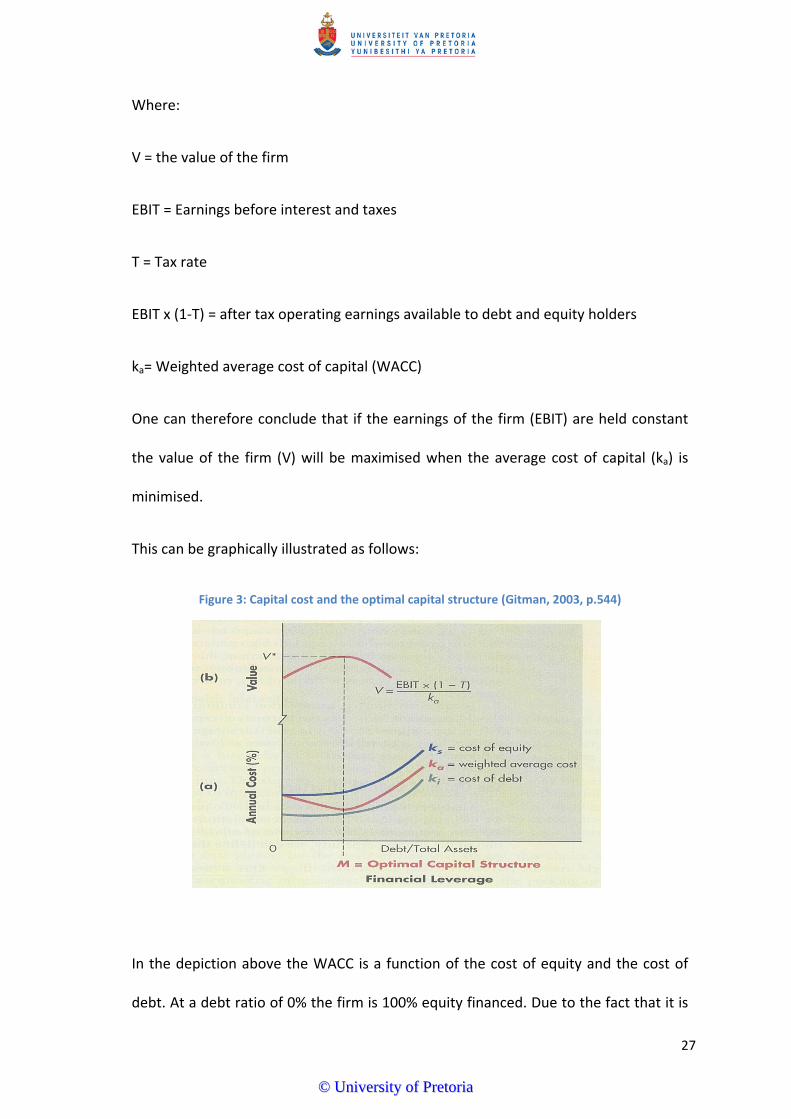
This can be graphically illustrated as follows:

Figure 3: Capital cost and the optimal capital structure (Gitman, 2003, p.544)

In the depiction above the WACC is a function of the cost of equity and the cost of

debt. At a debt ratio of 0% the firm is 100% equity financed. Due to the fact that it is

27


generally cheaper to employ debt financing than equity financing (ki<ks) the WACC

declines as more debt is added to the capital structure. As more debt is added costs

associated with debt begin to increase and the WACC starts to increase forming a U

shape or inflection point beyond which it is no longer sensible or economically viable

to add debt to the capital structure of the firm (Gitman, 2003).

2.4.2.1. The advantages of debt

2.4.2.1.1. Interest tax shield

Because interest is deductible from profits the judicious use of debt can decrease the

firm’s tax liability and therefore increase its after‐tax free cash flow (Barclay & Smith,

2005). The value of the debt tax shield is a function of the amount of interest the firm

pays and its marginal tax rate (Opler, Saron & Titman, 1997).

2.4.2.1.2. Reduction of agency cost

In the most basic form of the agency cost problem managers may not act in the best

interest of shareholders especially when excessive free cash flows are present

choosing to spend cash on corporate empire building, consumption of (self‐

appointed) perks, making overpriced acquisitions or generally failing to operate

efficiently. In the aforementioned cases both debt and the payment of dividends may

be used as tools for disciplining managers (Graham & Harvey, 2001).

2.4.2.1.3. The benefit of debt in controlling overinvestment

The overinvestment problem occurs when managers invest the free cash flow of the

firm in projects that have returns below the firm’s cost of capital. It may be the result

28


of investing unprofitably in growth in the firm’s core business, or worse, diversifying

into unknown business areas. Contractually obliged interest and principal payments,

as a result of incurring debt, may in such cases crowd out excess capital problems

(Barclay & Smith, 2005). This could be achieved by paying out excess free cash as

dividends to the shareholders of the firm and borrowing to fund the growth projects

of the firm. In such cases debt will serve as a disciplining tool ensuring that

investment decisions and their implications are fully considered prior to committing

to the projects in question.

2.4.2.2. The cost of debt

2.4.2.2.1. Cost of financial distress

One of the major benefits proposed by the trade‐off theory is the interest tax

deductibility of debt. However should the firm go through a period of operating at a

loss the value of the interest tax shield will be reduced to zero but the burden of

interest expenses will only serve to increase the financial distress experienced by the

firm.

2.4.2.2.2. Agency cost

Agency costs are defined as costs that occur as a consequence of conflicts of interest

and can originate as a result of conflicts between the managers and owners of firms

or the debt holders and equity holders of firms (Harris & Raviv, 1991).

Manager‐Shareholder: According to Ryen et al (1997) the two most prevalent areas

of manager‐shareholder conflict can be seen in the unwillingness of managers to

leverage the firm to its optimal value thereby forgoing significant shareholder value

29


and overspending on management perquisites. In instances where there is excessive

free cash flow debt can serve as a tool to discipline management.

Shareholder‐debtor: There is a variety of ways in which management may favour

shareholders above debt holders thereby transferring wealth from debt holders to

the owners of the firm. This could be achieved by issuing new debt with a higher

priority than the existing debt, rejecting positive Net Present Value projects if the

benefits will accrue only to debt holders, and at the extreme, through perverse

dividend pay‐outs at the risk of liquidating the firm. In order to protect themselves

debt holders can introduce protective covenants into their loan agreements. It should

however be noted that these covenants can lead to underinvestment, finance and

production problems (Ryen, Vasconcellos & Kish, 1997).

2.4.2.2.3. The underinvestment problem

Companies have a tendency to under invest when they face financial difficulty such as

the inability to service its debt (principal and interest) repayments. (Barclay & Smith,

2005). This problem is further accentuated when potential equity investors are

deterred by the fact that much of their equity investment will not go towards

creating wealth for them but rather will be applied to restore the financial position of

the firm’s debt holders. In such cases the cost of equity would be so excessive (deeply

discounted) that managers may choose to forgo profitable investment opportunities

(Myers, 2001; Barclay & Smith, 2005).

30


In addition to forgoing positive Net Present Value projects management may also

forgo adequate company specific investment in its human resources (Ryen et al,

1997).

2.4.2.3. The dynamic trade‐off theory

Unlike the static trade‐off theory, which implicitly assumes that firms always stay at

target leverage by continuously adjusting leverage to the target, the dynamic version

recognizes that financing frictions make it suboptimal for firms to continuously adjust

their leverage to the target. Under the dynamic trade‐off theory, firms weigh the

benefit of adjusting their capital structures against the adjustment cost and make

leverage adjustments only when the benefit outweighs the cost (Ovtchinnikov, 2010).

This means that should market conditions be unfavourable, firms may spend

considerable time away from their target capital structures and only revert to them

when conditions are favourable. Whether a firm is above or below its target leverage

ratio will also impact the speed with which it returns to its target capital structure.

The reason for this may be that once a firm operates at a level of debt significantly

above the industry mean the cost of financial distress increases markedly and the act

of rebalancing its capital structure becomes a more meaningful task (Cai & Gosh,

2003).

Myers (1984) indicates that he is not fully satisfied with the explanation of a dynamic

trade‐off theory insofar as frictions that prevent firms from staying at or near their

ideal capital structure are not mentioned to be of first order concern in the static

trade‐off theory. Should costs be so large that it could serve to force managers to

31


take extended excursions away from their optimal capital structure, more time

should be spend on understanding and explaining these frictions rather than refining

the static trade‐off theory (Myers, 1984).

2.4.3. Pecking order theory

According to the pecking order theory firms have no well‐defined target debt/equity

ratio and each firm’s observed debt ratio simply reflects the firm’s cumulative

requirement for external finance over an extended period (Myers, 1984). According

to the pecking order model firms will first use internal funds (retained earnings)

before issuing debt and will finally only issue equity under duress or when the

investment requirement so far exceed debt capacity that it would lead to excessive

leverage (Fama & French, 2005).

Just as is the case with trade‐off theory the pecking order has an intuitive appeal but

it is not without challenges however.

Although the pecking order theory is grounded on adverse selection based on

information asymmetry, it is not necessary for information asymmetry to exist for a

financing hierarchy to arise, other factors such as the expense of issuing various

classes of securities and incentive conflicts can create their own pecking orders (Leary

and Roberts, 2010). This view is supported by Titman and Wessels (1988) who found

that transaction cost may be an important determinant of capital structure choice;

32


this is reflected in the fact that short‐term debt ratios are negatively related to firm

size. This is probably related to the relatively high transaction cost of issuing long

term financial instruments such as bonds for smaller firms.

According to Myers (2001) practitioners usually think of the cost of external finance

as that of administration and underwriting and in some instances the under‐pricing of

new securities however asymmetric information creates the possibility that there

might also be a cost related to not accepting positive net present value (NPV)

projects. One such cost may be that the shareholders of the firm could conclude that

managers are excessively risk adverse thereby failing to adequately represent

shareholder interest. Managers on the other hand may feel that they have better

information about the cost and benefits of debt than shareholders thereby choosing

to forgo new investment opportunities especially if the earnings of the firm or

investment project is volatile (Lewellen, 2006).

Even if a pecking order do exists, companies may at times choose to ignore it in order

to maintain a spare debt capacity or to retain internal funding in favour of debt if

they believe that it will be required to fund attractive future investment

opportunities (Ryen et al, 1997). Shivdasani and Zenner (2005) state that one reason

companies may choose to maintain spare debt capacity is to maintain their credit

ratings since it can take several years to recover from a downgrade. Spare debt

capacity improves a company’s ability to withstand a period of poor performance and

allows it to execute a recovery plan.

33


2.4.4. The market timing theory of capital structure

Equity marketing timing refers to the practise of issuing shares when equity

valuations are high relative to book and past market valuations and repurchasing

equities when their market values are low. As a consequence observed capital

structures are a function of the past market values of securities rather than a desire

to achieve an optimum capital structure or as a consequence of following a pecking

order (Baker & Wurgler, 2002).

Baker and Wurgler (2002) point to four outcomes of empirical studies that support

their market timing hypothesis:

I. Past analysis of financing decisions indicate that firms issue equity instead of debt

when share prices are high relative to book and past market values and tend to

repurchase shares when the market values are low compared to historic averages

II. Analyses of long‐run stock returns following corporate finance decisions suggest that

timing the equity market is successful (for firms) on average

III. Earnings forecasts and realisations around equity issues suggest that firms issue

equity when there is investor market optimism about future earnings prospects (and

investors are hence likely to overpay for those equities)

IV. Finally and most convincingly two thirds of Chief Financial Officers (CFOs) admit to

market timing in anonymous surveys

34


DeAngelo, DeAngelo and Stulz (2010) do however pose a serious empirical caveat to

market timing theorist: most firms with attractive market timing opportunities fail to

issue stock. One reason proposed for this failure to issue stock is the fact that

investor rationality would force managers to disguise attempts to sell overvalued

stock. Rational and alert investors would immediately recognise any attempts to sell

overvalued stock and as a consequence reduce the price they are prepared to pay for

the stock. Another explanation is the fact that managers may simply not be able to

time the market as is proposed by Baker and Wurgler (2002). De Angelo et al (2010)

states that this explanation seems to be especially compelling in the light of recent

events where prominent financial institutions (Lehman Brothers, AIG, Bear Stearns

etc.) all repurchased shares at high prices immediately preceding the 2008 financial

meltdown.

DeAngelo et al (2010) states the primary reason for issuing stock is to fund the firms

near term cash needs with market timing playing only an ancillary role in the

decision. According to their findings 81% of all firms would have subnormal cash

levels and 62% would run out of cash within one year if they failed to engage in a

seasoned equity offering.

2.5. Financial distress

Traditional capital structure theory holds that a reasonable or moderate amount of

debt incurred by profitable firms will reduce the overall cost of capital of the firm and

hence increase firm value. Once the level of debt moves beyond the optimal debt

35


point the cost of capital and the financial risk associated with the firm will increase

and the value of the firm will decrease and the likelihood of financial distress

increases (Ariff, Hassan & Shamsher, 2008). Highly levered firms are more likely to

become distressed however the margin between highly levered and acceptable

leverage levels may not be significant especially in the light of external economic

shocks. Examples of this can be found in the Asian financial crisis. Prior to the Asian

crisis the difference between the debt ratio of firms that became distressed and

healthy firms was .0167 and .0108 respectively. After the financial crisis the debt level

of distressed firms rose to 0.627‐0.740 while that of healthy firms increased to 0.350‐

0.423. A limitation of previous capital structure research is the fact that the linkage

between healthy firms becoming financially distressed after financial shocks has been

under explored (Ariif et al, 2008). Indirect support for this finding is provided by

Zaher (2010) who found that debt free firms outperformed their indebted peers in

both the long and short run. Investors also penalised firm with high debt levels while

rewarding those firms that had no debt on their balance sheets following financial

crisis (Zaher, 2010). This result stands in direct contrast to the optimal capital

structure theory and may be interpreted as offering support for the pecking order

theory.

Financial distress refers to the costs that are incurred as a consequence of

bankruptcy, the efforts to avoid bankruptcy, the need to reorganise or the agency

cost that is incurred when the credit worthiness of a firm is in question (Myers, 2001).

36


Financial distress costs can be classified as either a direct or an indirect insolvency

cost (Firer et al, 2008).

Direct costs are those cost that are incurred either as a consequence of insolvency

procedures or in the efforts of reorganisation. Although the primary costs here are

legal and administrative costs there are also costs related to the dissipation of value

of the firm’s assets under bankruptcy procedures (Firer et al, 2008, Gitman 2003).

Indirect costs are far broader and more difficult to measure but includes factors such

as the under and overinvestment problems and the disengagement of the various

stakeholders of the firm.

Until such a time that the firm has been declared insolvent through legal proceedings

the shareholders own the firm and the assets of the firm and will be reluctant to

hand over ownership to debt holders that have a priority claim on the assets of the

firm. This might force the firm to invest in excessively risky projects in an effort to

save the firm; known as the overinvestment problem. Bondholders on the other hand

will act in their economic self‐interest and will try to protect the value of their legal

claim to the assets of the firm leading to an underinvestment problem.

There is also a possibility that the customers, suppliers and employees of the firm will

be reluctant to continue doing business with a financially distressed firm resulting in

further indirect costs.

Finally in trying to avoid insolvency the management of the firm will be distracted

from their normal operational and strategic functions leading to lost sales and

investment opportunities.

37


2.6. The capital structure landscape

Figure 4 below provides a conceptual overview of the factors impacting on or

influencing capital structure decisions.

Figure 4: Conceptual overview of capital structure landscape (adapted from Rayan, 2008)

Observed capital structure of the firm

Preffered capital structure of the firm

Pecking order theory

Trade‐off theory

Information asymmetry theory

Agency cost theory

Short term financing needs

Availability of profitable projects

The centre of the figure indicates the optimal capital structure range for a firm. The

observed capital structure may or may not be in this optimal capital range. One

example of a firm not being within the optimal capital structure range could be that

of a firm experiencing financial distress another may be the case of a firm operating

without any debt in its capital structure. Most firms with a target capital structure will

spend a substantial amount of time away from its target capital structure. This

departure from the ideal capital structure could be as a consequence of changes in

38


equity valuation or market friction or investment opportunities. The firm is however

assumed to take certain actions over time that will move it toward its target capital

structure.

Immediately outside the optimal capital structure range are a number of factors

impacting on the decision about what would constitute an ideal capital structure or

optimal capital structure range. Here it is possible to distinguish between two types

of factors: firstly purely theoretical constructs that are assumed to influence or guide

the practitioners and secondly practical aspects such as the availability of investment

opportunities and short term funding needs.

The next level indicates firm specific factors that include factors such as the maturity

of the firm (life cycle theory), profitability, and money spent on tangible versus

intangible assets etc.

The second outer most ring constitutes industry specific factors. This includes the

volatility of the industries revenues, typical debt/equity ratios etc.

The final level is the macro environment in which the firm operates and constitutes

all the macro‐economic realities faced by the firm as well as the legal and political

environment. Factors such as the rate of exchange volatility would form part of this

environment.

From the model above it should be clear that the capital structure decision is not a

simple one and a failure to understand the environment in which these decisions are

made could lead to flawed assumptions.

39


2.7. Conclusion

Firms (or the managers of firms) are largely free to choose any capital structure they

want especially since capital structure decisions can be made independently from

investment decisions. Capital structure decisions can however have important

implications for the value of the firm and its cost of capital (Firer et al, 2008).

In this chapter we reviewed the three most prevailing capital structure theories

namely the trade‐off theory, the pecking order theory and the market timing theory.

The trade‐off theory suggests that there is an optimal level of debt that balances the

advantages of debt against the costs of debt. It must be noted however that theory is

able to give precious little advice to practitioners about the calculation of an optimal

debt/equity ratio. Factors such as external economic shocks may also have a bigger

than expected impact on firms with comparatively similar leverage levels even if

academics regard these firms as conservatively leveraged. A prime example of this is

the relatively small differences that existed in the leverage ratios of both healthy and

distressed firms prior to the Asian crisis. This might indicate that operational factors

are at least as important as leverage levels when designing an optimal capital

structure.

Pecking order theory suggests that there is a financing hierarchy that starts with

retained earnings before moving to low cost debt and finally expensive equity. The

pecking order theory is based on a special case of information asymmetry namely

adverse selection cost. An unanswered question for the pecking order theory remains

the desire for management to maintain spare debt or funding capacity thereby

violating the pecking order theory in favouring debt over retained earnings.

40


The market timing theory suggests that managers will issue a specific type of security

when it believes that the security is overpriced or when market conditions are

favourable. A major flaw with this theory is that there is ample evidence of managers

mistiming the market suggesting that the theory, although desirable, may not be

practically feasible.

Following this literature review the researcher has to concur with the statement by

Ryen et al (1997, pg 48) that “there is much room for improvement in the

explanatory and predictive ability of capital structure theory”.

41


3. Chapter Three – Research questions and hypothesis

3.1. Research hypothesis one: the relationship between profitability and debt

The trade‐off and pecking order theories differ in their predictions on firm

profitability and the amount of leverage incurred by firms.

According to the trade‐off theory profitable firms will make greater use of debt in

order to capture the benefit of the tax shield offered by debt. In addition to the tax

shield benefit more profitable firms may also impose the discipline of debt on

managers in order to reduce agency cost problems. The trade‐off theory predicts a

positive relationship between profitability and leverage. However the evidence is

mixed at best with more profitable firms having either insignificantly more debt at

best or having less debt in their capital structures (Barclay & Smith, 2010).

The pecking order theory predicts that profitable firms will make use of retained

earnings as their primary source of funding and only if a funding deficit exists will

they make use of debt and then equity.

In order to deal with the different predictions of the trade‐off and pecking order

theories the research hypotheses has been stated twice. First to test for the positive

correlation between leverage and profitability suggested by the trade‐off theory and

secondly to test for the negative correlation between leverage and profitability

suggested by the pecking order theory.

42


Research Hypothesis 1A:

H0a = ρleverage,profitability ≤ 0 (Profitability and leverage is not correlated or negatively

correlated)

H1a = ρleverage,profitability > 0 (Profitability and leverage is positively correlated)

Research hypothesis 1B:

H0b = ρleverage,profitability ≥ 0 (Profitability and leverage is not correlated or positively

correlated)

H1b = ρleverage,profitability < 0 (Profitability and leverage is negatively correlated)

3.2. Research hypothesis two: difference between industry median debt levels

Capital structure theory suggests that the industry to which a firm belongs is likely to

have a considerable impact on the observed leverage levels of individual firms and

that over time firms will tend to migrate toward the median industry debt levels. This

movement toward the industry median debt level is regarded as evidence that an

optimal capital structure does exist (Bowen, Daley & Huber, 1982).

Although this research does not specifically test for the migration toward industry

median debt levels over time the existence of both statistically and practically

significant differences in median industry debt levels may be interpreted as support

for the optimal capital structure theory.

H0 = μ1 = µ2 = …μ8 (Industry median debt levels are homogenous)

H1 = μ1 ≠ µ2 ≠ …μ8 (Industry median debt levels are heterogeneous)

43


3.3. Research hypothesis three: the relationship between earnings volatility

and debt

Both the trade‐off theory and pecking order theory predicts that firms with higher

earnings volatility should make more conservative use of leverage in their capital

structures in order to prevent potential financial distress caused by the inability to

meet their financial obligations. According to the trade‐off theory firms weigh the

benefits of debt against the potential cost of debt in an effort to maximise

shareholder wealth.

The pecking order theory predicts that firms with more volatile earnings will preserve

spare debt capacity in an effort to prevent them from issuing more costly debt at a

later stage.

Regardless of which theory is correct the relationship between earnings volatility and

the observed capital structure of the firms is of practical significance in an

environment characterised by an increasing volatility in currency and commodity

prices. In such an environment managers are expected to be both prudent in their

financial management practises and proactive in their risk management strategies

(Shivdasani & Zenner, 2005).

H0 = ρleverage,stdev ROA ≥ 0 (There is no correlation between debt and earnings volatility)

H1 = ρleverage,stdev ROA < 0 (Earnings volatility and debt is negatively correlated)

44


3.4. Research hypothesis four: the relationship between the price‐to‐book

ratio and debt

The value of a firm’s future opportunities can be estimated by observing the firms

market to book ratio. The book value is the value of the firm’s assets in place, net of

liabilities and is backward looking (i.e. based on historic accounting values). The

market value is an estimation of the firm’s growth opportunities as perceived by

investors. Empirically there has been a strong inverse relationship between market‐

to‐book ratios and leverage levels or debt ratios (Myers, 2002). Booth, Aivazian,

Demirguc‐Kunt and Maksimovic (2001) however question the portability of all the

elements of capital structure theory specifically noting the price‐to‐book ratio as an

exception to the rule. According to them the price‐to‐book ratio can vary widely in

developing countries.

This hypothesis will therefore test to see if this relationship holds true in the South

African context.

H0 = ρleverage,p/book ≥ 0 (leverage and the price‐to‐book ratio is not correlated)

H1 = ρleverage,p/book < 0 leverage and the price‐to‐book ratio is negatively correlated)

3.5. Research hypothesis five: the relationship between debt and the

probability of financial distress

Opler et al (1997) states that firms with highly levered balance sheets are likely to

suffer disproportionately during economic downturns and as a consequence are

more likely to become financially distressed that their lower levered counterparts.

45


This view is supported by Shivdasani and Zenner (2005) who states that firms with

little debt on their balance sheets will continue to service their debt obligations even

in the face of significant financial and economic shocks while highly levered firms

would see their cash flow ratios plummet, perhaps to the point of being unable to

meet their obligations. This research hypothesis therefore aims to test whether firms

that made aggressive use of debt finance (i.e. was in the upper 50 percentile of

indebted firms) have financial distress scores that differ statistically from those firm

that made conservative use of debt following the onset of the global financial crisis.

H0 = ρfin distress,D/E ≤ 0 (the financial distress score of firms making aggressive use of

debt is no different than firms making conservative use of debt financing in their

capital structures)

H1 = ρfin‐distress,D/E > 0 (the financial distress score of firms making aggressive use of

debt is greater than firms making conservative use of debt financing in their capital

structures)

46


4. Chapter four ‐ Research Methodology

4.1. Introduction

According to Cameron and Price (2009) research is about collecting relevant data and

extracting from that data the relevant information to support an argument or draw

valid conclusions.

Chapter four discusses the research process and methodology that was employed to

answer the research hypotheses defined in chapter three.

4.2. Population of relevance

The population of relevance was all companies listed on the main board of the

Johannesburg Stock Exchange over the ten year period from 1999 to 2007.

The following firms were specifically excluded from the study:

a. AltX listed companies – due to the fact that AltX listed companies have very different

listing requirements from that of the main board of the Johannesburg Stock

Exchange, lower volumes traded and significantly lower market capitalisation it was

decided to exclude this sector.

b. The financial sector was excluded due to the fact that there is a separate strand of

literature dealing specifically with the capital structure of the financial industry. Banks

are bound by a host of regulations that non‐financial firms are not subjected too,

they are also incentivised to maximise leverage up to the regulatory minimum (Gropp

and Heider, 2009).

47


The following firms were excluded from the study:

A firm for which the debt‐to‐equity ratio data over the full ten year period was not

available was excluded from the study. This means that all firms that were

suspended, de‐listed or not yet listed at 1 January 1998 were specifically excluded

from the study.

4.3. Unit of analysis

The unit of analysis was a single company listed on the Johannesburg Stock Exchange

over the period ranging from 1999 until 2009. This is in line with previous empirical

studies conducted on capital structure.

4.4. Sampling Method

The sample may be regarded as a convenience sample as firms were selected or

excluded based on whether they fulfilled the desired criteria of the researcher.

Analysis was also conducted on industry segments in an attempt to observe

differences in the capital structure choices of different industries therefore the

sample may be regarded as stratified. Since the number of firms in each industry

segment is not the same the result was a disproportional stratified sample. (Zikmund,

2003 pg. 388)

4.5. Data collection process

Only secondary data was used in this study. The primary source for data was the

McGregor BFA (2010) research domain database.

48


4.6. Data analysis process

4.6.1. Descriptive statistics

The transformation of data into a format that is easier to understand and interpret is

known as descriptive statistics (Zikmund, 2003). According to Pallant (2009)

descriptive statistics can be used to:

a) Describe the characteristics of your sample

b) Checking your variables to ensure that they do not violate the underlying statistical

techniques that you intend using to answer your research questions

c) To address specific research questions

The first step will therefore be to describe the sample using descriptive statistics. In

addition to graphs and tables the following descriptive statistics will be used to

describe the sample

4.6.1.1. Measures of central tendency

4.6.1.1.1. The sample mean

The mean is also known as the arithmetic average of the sample or the sum of all the

observations divided by the number of observations. The formula for the mean is:

Equation 3: Sample mean (Albright et al, 2006 pg. 82)

Where:

49


Σ = Sigma or summation sign

n = number of observations

i = the value of the observation, therefore Xi is the value of the ith observation

4.6.1.1.2. The median

The median is the centre or middle observation of the data set. In the case of an

equal number of observations it is the average of the two centre observations.

4.6.1.2. Measures of dispersion

4.6.1.2.1. The minimum, maximum and range

The minimum is the smallest value it the data set and the maximum is the largest

observation in the data set. The range is the difference between the minimum and

maximum values.

4.6.1.3. Measures of variability

4.6.1.3.1. Variance

The variance is the average of the squared deviations from the mean.

4.6.1.3.2. Standard deviation

Standard deviation is defined as the square root of the variance and is expressed in

the original units of measure. The relationship between the standard deviation and

variance can be expressed as:

Equation 4: The relationship between standard deviation and variance (Albright et al, 2006 pg. 87)

50


4.6.1.4. Distribution of data

Many statistical tests assume data is normally distributed. The term normality is used

to describe outcomes that are represented by a symmetrical bell shaped curve with

the greatest frequency of scores in the centre and reduced frequencies toward the

extremes of the curve (Pallant, 2007). Normality can therefore partially be

ascertained by obtaining the skewedness and kurtosis values of the data distribution

as well as by visually inspection the data distribution (histogram).

4.6.2. Exploring the relationships between variables

4.6.2.1. Independent samples T‐test

T‐test may be used to determine if there are statistically significant differences

between the means of two samples or groups (Zikmund, 2003). T‐test may be used

for independent or paired samples test that are normally distributed. In the event

that data does not conform to the requirement for normality the non‐parametric

Mann‐Whitney U or Wilcoxon signed‐rank test for determining the differences in the

median between groups may be used (Pallant, 2008).

Table two below illustrates the decision making process followed in deciding upon

the appropriate test to determine whether a statistically meaningful difference exist

between the means of two groups:

51


Table 2: Selection matrix for the appropriate test for differences between the mean values of two groups (from Gibs class notes)

Normal Equal Variance

Yes Yes Equal‐Variance T‐Test T‐value

Yes No Aspin‐Welch Unequal‐Variance Test T‐value

No Yes

Mann‐Whitney U or Wilcoxon Rank‐

sum test for difference in medians

Rank‐Sum Test for Difference Z‐value

No No

Kolmogorov‐Smirnov test for

different distributions Dmn criterion value*

Appropriate test

statistic reported by NCSS 2007®

Data Characteristics Appropriate difference test

reported by NCSS 2007®

* Maximum difference between two empirical distribution functions

All t‐test will be conducted by firstly preparing and sorting the relevant data. During

the preparation phase all missing data and outliers will be corrected or deleted, once

this has been done the data will be sorted in descending order according to the

independent variable. The dependant variable will then be divided into two equal

groups in order to compare the means or medians of the groups. Prior to comparing

the means the data will be checked for the assumption of normality in order to

ensure that the appropriate statistical test for the difference between means or

medians are used for hypothesis testing.

4.6.2.2. Correlation analysis

The study of the relationship between two variables is referred to as correlation

analysis and is one of the most persuasive statistical tools used to analyse data. The

relationship between the variables can be linear, non‐linear or non‐existent it is

therefore useful to use scatter plots top identify potential relationship that might not

be otherwise obvious.

Correlations are numerical summary measures of strength of the relationship

between two variables and can vary between a perfect positive correlation (+1) to a

52


perfect negative correlation (‐1). A value approximating 0 indicates that there is no

relationship between the variables in question. One of the drawbacks of correlation

analysis is the fact that is cannot be used to establish causation amongst variables, or

stated differently, state that a change in the independent variable will lead to a

change in the dependant variable.

Correlation analysis will be used to support the findings of the t‐test in this research

project.

4.6.2.3. One way analysis of variance (ANOVA)

The one way analysis of variance is an appropriate statistical tool to measure the

difference between means for more than two groups when there is only one

independent variable affecting all groups. The null hypothesis states that all means

are equal. Should there be significant differences between the groups, in terms of

behaviour or characteristics; there will be statistically significant variances of the

group’s means about a grand mean. The null hypothesis (assuming all means are

equal) will be rejected if at least two means vary from the central mean (Zikmund,

2003).

4.6.2.4. Parametric versus non‐parametric test

Statisticians generally make use of two types of test, parametric and non‐parametric

each with its own advantages and disadvantages. Parametric tests make a number of

53


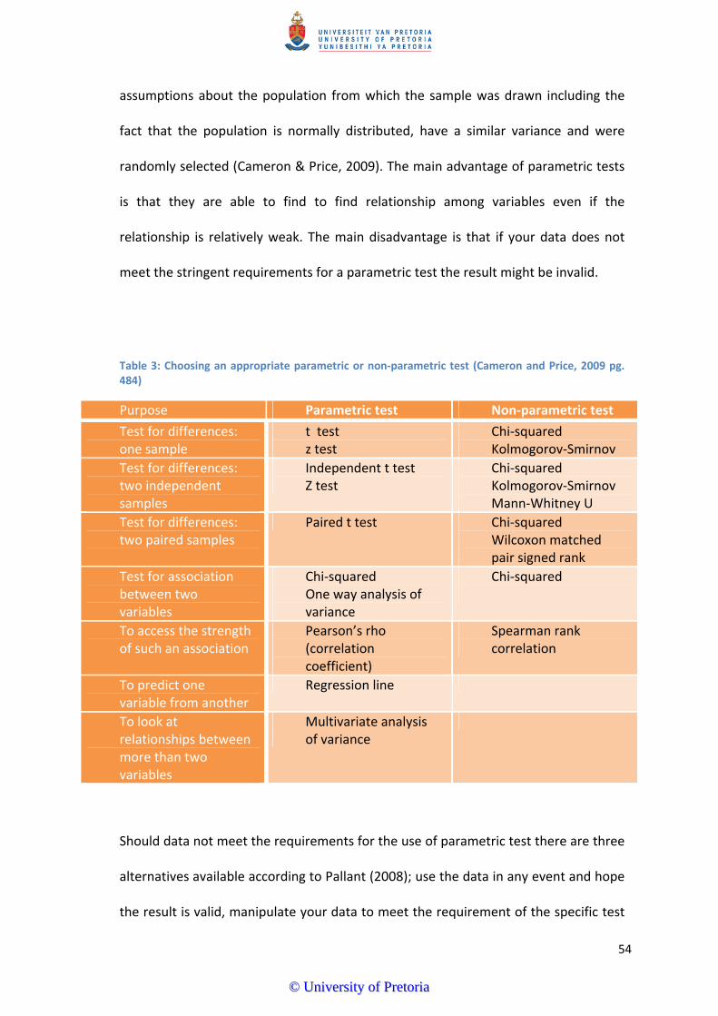
assumptions about the population from which the sample was drawn including the

fact that the population is normally distributed, have a similar variance and were

randomly selected (Cameron & Price, 2009). The main advantage of parametric tests

is that they are able to find to find relationship among variables even if the

relationship is relatively weak. The main disadvantage is that if your data does not

meet the stringent requirements for a parametric test the result might be invalid.

Table 3: Choosing an appropriate parametric or non‐parametric test (Cameron and Price, 2009 pg. 484)

Purpose Parametric test Non‐parametric test

Test for differences: one sample

t test z test

Chi‐squared Kolmogorov‐Smirnov

Test for differences: two independent samples

Independent t test Z test

Chi‐squared Kolmogorov‐Smirnov Mann‐Whitney U

Test for differences: two paired samples

Paired t test Chi‐squared Wilcoxon matched pair signed rank

Test for association between two variables

Chi‐squared One way analysis of variance

Chi‐squared

To access the strength of such an association

Pearson’s rho (correlation coefficient)

Spearman rank correlation

To predict one variable from another

Regression line

To look at relationships between more than two variables

Multivariate analysis of variance

Should data not meet the requirements for the use of parametric test there are three

alternatives available according to Pallant (2008); use the data in any event and hope

the result is valid, manipulate your data to meet the requirement of the specific test

54


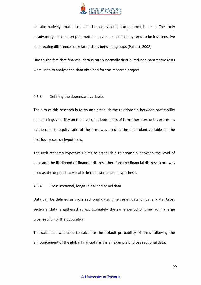
or alternatively make use of the equivalent non‐parametric test. The only

disadvantage of the non‐parametric equivalents is that they tend to be less sensitive

in detecting differences or relationships between groups (Pallant, 2008).

Due to the fact that financial data is rarely normally distributed non‐parametric tests

were used to analyse the data obtained for this research project.

4.6.3. Defining the dependant variables

The aim of this research is to try and establish the relationship between profitability

and earnings volatility on the level of indebtedness of firms therefore debt, expresses

as the debt‐to‐equity ratio of the firm, was used as the dependant variable for the

first four research hypothesis.

The fifth research hypothesis aims to establish a relationship between the level of

debt and the likelihood of financial distress therefore the financial distress score was

used as the dependant variable in the last research hypothesis.

4.6.4. Cross sectional, longitudinal and panel data

Data can be defined as cross sectional data, time series data or panel data. Cross

sectional data is gathered at approximately the same period of time from a large

cross section of the population.

The data that was used to calculate the default probability of firms following the

announcement of the global financial crisis is an example of cross sectional data.

55


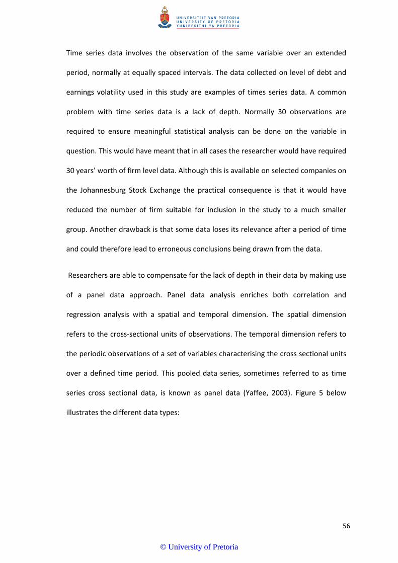
Time series data involves the observation of the same variable over an extended

period, normally at equally spaced intervals. The data collected on level of debt and

earnings volatility used in this study are examples of times series data. A common

problem with time series data is a lack of depth. Normally 30 observations are

required to ensure meaningful statistical analysis can be done on the variable in

question. This would have meant that in all cases the researcher would have required

30 years’ worth of firm level data. Although this is available on selected companies on

the Johannesburg Stock Exchange the practical consequence is that it would have

reduced the number of firm suitable for inclusion in the study to a much smaller

group. Another drawback is that some data loses its relevance after a period of time

and could therefore lead to erroneous conclusions being drawn from the data.

Researchers are able to compensate for the lack of depth in their data by making use

of a panel data approach. Panel data analysis enriches both correlation and

regression analysis with a spatial and temporal dimension. The spatial dimension

refers to the cross‐sectional units of observations. The temporal dimension refers to

the periodic observations of a set of variables characterising the cross sectional units

over a defined time period. This pooled data series, sometimes referred to as time

series cross sectional data, is known as panel data (Yaffee, 2003). Figure 5 below

illustrates the different data types:

56


Table 4: Example of panel data with time series and cross Sectional data highlighted

4.6.5. Financial ratios

4.6.5.1. Profitability

The return on total assets (ROA) is used as a scaled measure of firm profitability. It

measures the profitability of the firm relative to the firm’s investment in assets.

Return on total assets is defined as:

Equation 5: ROA (Firer et al, 2008 pg. 65)

The use of ROA to measure profitability is in line with previous studies conducted by

Titman and Wessels (1988) and Rajan and Zingales (1995).

4.6.5.2. Earnings volatility

57


Earnings volatility as measured as the standard deviation of the firm’s profitability

over the period of the study. Each year’s earnings are regarded as a separate data

point.

The use of the standard deviation of ROA is in line with previous studies conducted by

Titman and Wessels (1998).

4.6.5.3. Financial leverage

Financial leverage refers to the amount of debt used in the capital structure of the

firm relative to equity. Higher levels of leverage imply higher levels of debt in the

capital structure of the firm. The measure of leverage used in study is the debt/equity

ratio.

The debt to equity (D/E) ratio is defined as:

D/E =

Equation 6: Debt‐to‐equity ratio (Firer et al, 2008 pg. 60)

4.6.5.4. Financial distress probability

During 1968 Professor Edward I Altman from the University of New York introduced

the use of discriminant statistics to predict the likelihood of financial distress in firms.

The model made use of commonly available financial ratios to assign a Z score to

firms. The Z score is calculated as follows:

Z = 1.2X1 + 1.4 X2 + 3.3 X3 + 0.6 X4 + 1.0 XF

Equation 7: Altman Z score (Bodie, Kane & Marcus, 2009 pg. 470)

58


Where:

Z = Altman Z score

X1 = Working capital/total assets

X2 = Retained earnings/total assets

X3 = Earnings before interest and taxes (EBIT)/total assets

X4 = Market value of equity/book value of total liabilities

X5 = Sales/total assets

Firms assigned a score Z >2.99 is regarded as safe from financial distress while those

with a score of Z<1.81 was regarded as in the distress zone and likely to go bankrupt.

Firms with a score between 1.81 and 2.99 were regarded as being in the grey zone

with an uncertain outcome (Bodie et al, 2009).

4.6.6. Hypothesis testing

Theoretical hypothesis can be confirmed (or disconfirmed) by the application of

appropriate statistical techniques to empirical (observed) data (Zikmund, 2003).

The process of hypothesis testing is briefly outlined below:

I. The null hypothesis (H0) is defined

II. The alternative hypothesis (H1) is defined

59


III. The significance level or Alpha (α) is defined. The significance level determines the

probability level that is considered too low to offer support to the null hypothesis.

All tests were conducted at the α = 0.05 level (or the 95% confidence level)

IV. Based on the sample size and characteristics the appropriate statistical techniques

were chosen to determine whether the null hypothesis could be rejected in favour

of the alternative hypothesis based on the empirical data

4.7. Research limitations

4.7.1. Listed companies

The research in this study was done on a judgement sample of companies listed on

the Johannesburg stock exchange. Although judgement samples has the advantage

that it allows the researcher to select units for inclusion based on defined population

characteristics the disadvantage is that the sample might not be representative of the

population and the research outcome cannot be generalised to the population of

companies listed on the JSE.

Companies listed on the JSE also excludes privately owned firms and smaller

companies it would therefore be inappropriate to generalise the findings of this study

to these groups explicitly excluded in the research.

4.7.2. Survivorship bias

Survivorship bias refers to the act of skewing the results of a sample upwards due to

the fact that a number of firms would have failed over the period of the study have

60


been excluded from the study. In this study no attempt was made to compensate for

survivorship bias. The practical significance of this omission is the fact that, especially

in the case of the financial distress data, there would be a positive bias in the

outcome of the study.

4.7.3. Time period under consideration

Financial ratio data was collected for the period 1998‐2007. Financial distress

probability data was collected for the year 2009 (this is to allow for the lag effect

associated with financial distress as well as to compensate for the lag effect

associated with the accounting cycle). Due to changing market conditions it will be

inappropriate to expand the findings of this study to all other time periods.

4.7.4. Negative Debt/Equity ratios

All firms with negative Debt/Equity ratios were excluded from this study

4.8. Conclusion

Chapter four outlined the data collection process and research methodology that was

used to answer the five research questions stated in chapter three. In the next

chapter the data will be described and in chapter six the analysis of the data will be

discussed.

61


5. Chapter Five – Presentation of Results

5.1. Introduction

Chapter five is a summary of the results of the analysis conducted in accordance with

the guidelines presented in chapter four indicating the proposed research

methodology. The presentation of results is initiated by a general description of the

sample selected for inclusion in the study followed by a discussion of the

independent variable (capital structure as indicated by the D/E ratio). This is followed

by the outcome or the t‐tests and correlation analysis that were run using the NCSS

statistical package.

5.2. General information and descriptive statistics for the sample data

As of October 2010 the main board of the Johannesburg Stock Exchange comprised

342 companies classified into ten industries. Two of the ten industries, the financial

and utilities sectors were explicitly excluded from this research. The financial sectors

was excluded based on reserve requirements that skew their capital structures and

the utilities sector was excluded because there are no firms listed in this category.

In order to be included in the study firms had to have data available throughout the

period 1998‐2007 as well as a financial distress score for the year 2009. Any firm that

did not comply with this requirement was excluded from the sample.

All firms with negative debt‐to‐equity ratios or that had extreme outliers in their data

period were excluded as well. For the debt‐to‐equity ratio a value greater than nine

was considered to be an extreme outlier to be excluded.

62


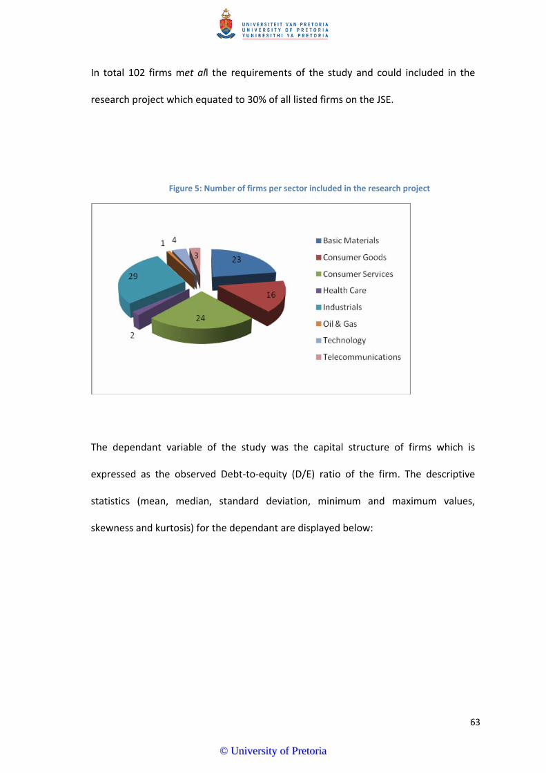
In total 102 firms met all the requirements of the study and could included in the

research project which equated to 30% of all listed firms on the JSE.

Figure 5: Number of firms per sector included in the research project

The dependant variable of the study was the capital structure of firms which is

expressed as the observed Debt‐to‐equity (D/E) ratio of the firm. The descriptive

statistics (mean, median, standard deviation, minimum and maximum values,

skewness and kurtosis) for the dependant are displayed below:

63


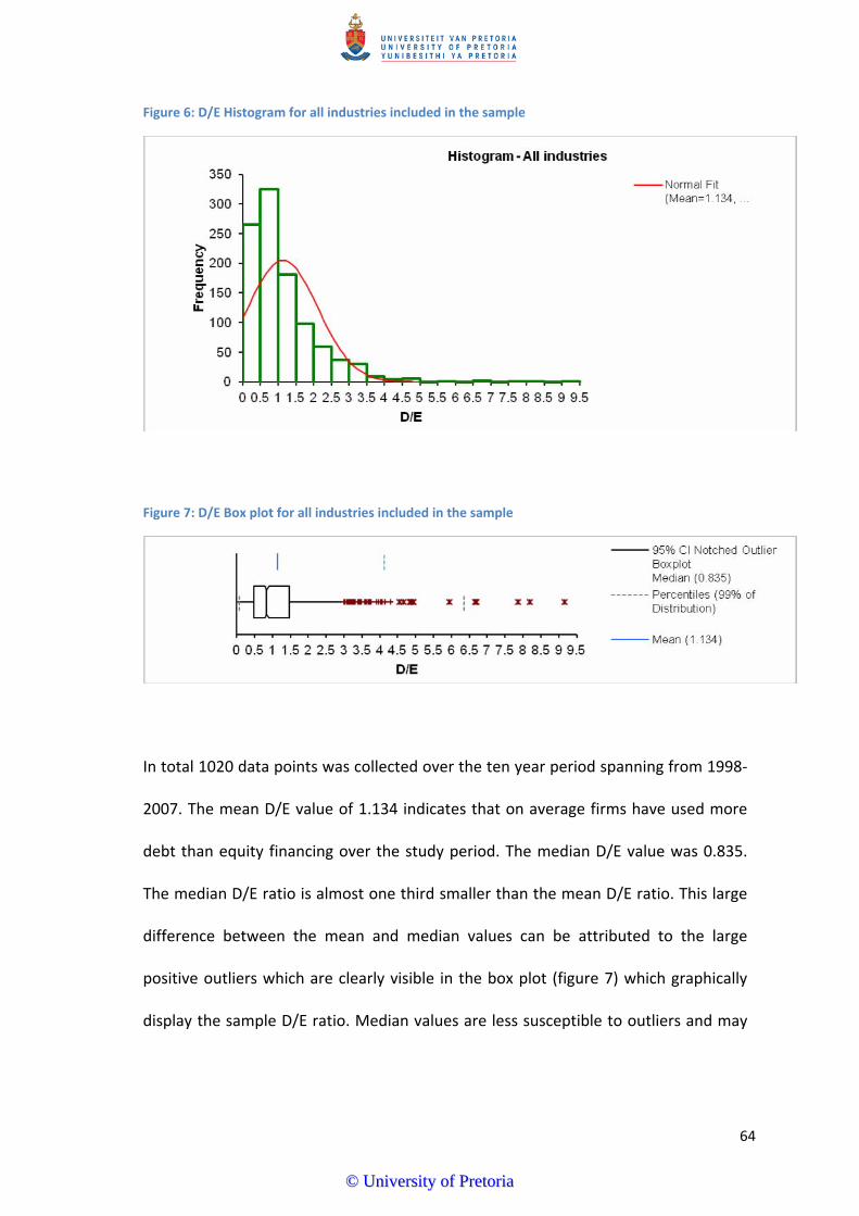
Figure 6: D/E Histogram for all industries included in the sample

Figure 7: D/E Box plot for all industries included in the sample

In total 1020 data points was collected over the ten year period spanning from 1998‐

2007. The mean D/E value of 1.134 indicates that on average firms have used more

debt than equity financing over the study period. The median D/E value was 0.835.

The median D/E ratio is almost one third smaller than the mean D/E ratio. This large

difference between the mean and median values can be attributed to the large

positive outliers which are clearly visible in the box plot (figure 7) which graphically

display the sample D/E ratio. Median values are less susceptible to outliers and may

64


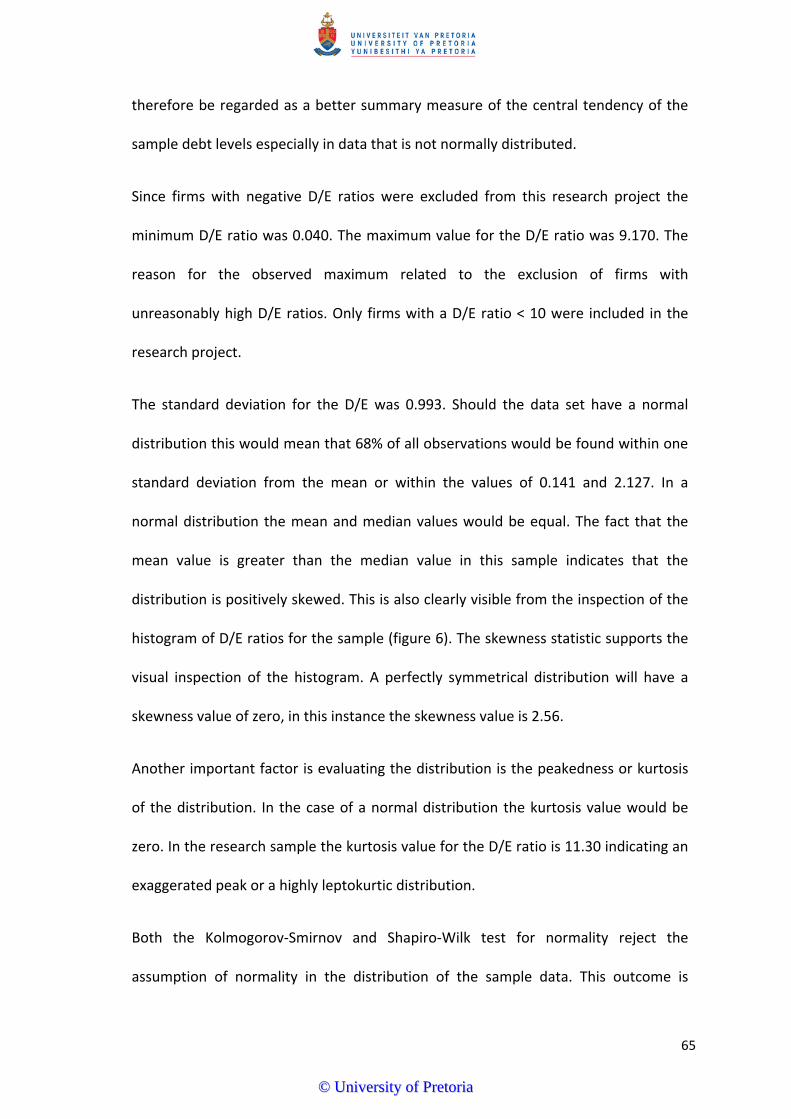
therefore be regarded as a better summary measure of the central tendency of the

sample debt levels especially in data that is not normally distributed.

Since firms with negative D/E ratios were excluded from this research project the

minimum D/E ratio was 0.040. The maximum value for the D/E ratio was 9.170. The

reason for the observed maximum related to the exclusion of firms with

unreasonably high D/E ratios. Only firms with a D/E ratio < 10 were included in the

research project.

The standard deviation for the D/E was 0.993. Should the data set have a normal

distribution this would mean that 68% of all observations would be found within one

standard deviation from the mean or within the values of 0.141 and 2.127. In a

normal distribution the mean and median values would be equal. The fact that the

mean value is greater than the median value in this sample indicates that the

distribution is positively skewed. This is also clearly visible from the inspection of the

histogram of D/E ratios for the sample (figure 6). The skewness statistic supports the

visual inspection of the histogram. A perfectly symmetrical distribution will have a

skewness value of zero, in this instance the skewness value is 2.56.

Another important factor is evaluating the distribution is the peakedness or kurtosis

of the distribution. In the case of a normal distribution the kurtosis value would be

zero. In the research sample the kurtosis value for the D/E ratio is 11.30 indicating an

exaggerated peak or a highly leptokurtic distribution.

Both the Kolmogorov‐Smirnov and Shapiro‐Wilk test for normality reject the

assumption of normality in the distribution of the sample data. This outcome is

65


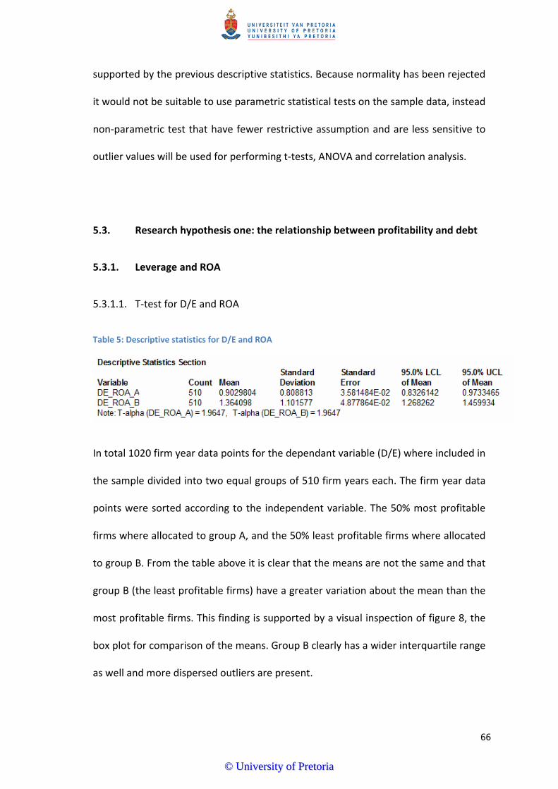
supported by the previous descriptive statistics. Because normality has been rejected

it would not be suitable to use parametric statistical tests on the sample data, instead

non‐parametric test that have fewer restrictive assumption and are less sensitive to

outlier values will be used for performing t‐tests, ANOVA and correlation analysis.

5.3. Research hypothesis one: the relationship between profitability and debt

5.3.1. Leverage and ROA

5.3.1.1. T‐test for D/E and ROA

Table 5: Descriptive statistics for D/E and ROA

In total 1020 firm year data points for the dependant variable (D/E) where included in

the sample divided into two equal groups of 510 firm years each. The firm year data

points were sorted according to the independent variable. The 50% most profitable

firms where allocated to group A, and the 50% least profitable firms where allocated

to group B. From the table above it is clear that the means are not the same and that

group B (the least profitable firms) have a greater variation about the mean than the

most profitable firms. This finding is supported by a visual inspection of figure 8, the

box plot for comparison of the means. Group B clearly has a wider interquartile range

as well and more dispersed outliers are present.

66


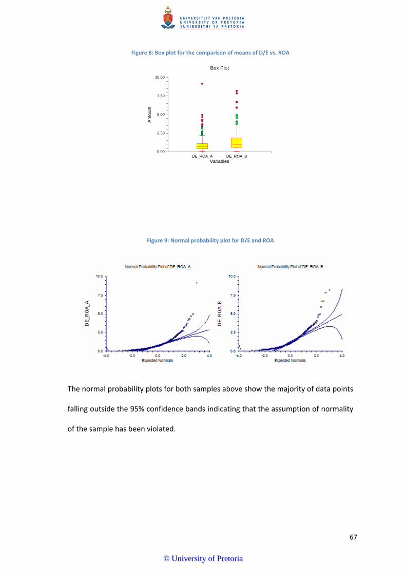
Figure 8: Box plot for the comparison of means of D/E vs. ROA

0.00

2.50

5.00

7.50

10.00

DE_ROA_A DE_ROA_B

Box Plot

Variables

Am

ount

Figure 9: Normal probability plot for D/E and ROA

The normal probability plots for both samples above show the majority of data points

falling outside the 95% confidence bands indicating that the assumption of normality

of the sample has been violated.

67


Table 6: Test of assumptions of normality for D/E and ROA

The findings from the visual inspection of the normal probability plot is confirmed by

the test of assumptions section of the NCSS output. Both samples violate the

skewness, kurtosis and omnibus normality test. Equal variances have also been

rejected using the modified‐Levene equal variance test for non‐parametric data.

Due to the fact that normality in the data distribution has been rejected the non‐

parametric Mann‐Whitney U test was used to test for the differences between

means. The Mann‐Whitney U test is used when assumption of normality is not valid

but permitting the distributions are at least ordinal in nature and that they are

identical except for the measure of central tendency.

Table 7: Test for the differences between means for D/E versus ROA

68


Test of hypothesis.

Research hypothesis 1A:


correlated)


The null hypothesis could not be rejected. The probability value (p‐value) exceed the

pre‐defined significance level for this test (α = 0.05)

Research Hypothesis 1B:


correlated)


As the probability level (p‐value) is smaller than the specified significance level (α =

0.05) the null hypothesis stating that there is no correlation or a positive correlation

between profitability and leverage is rejected.

69


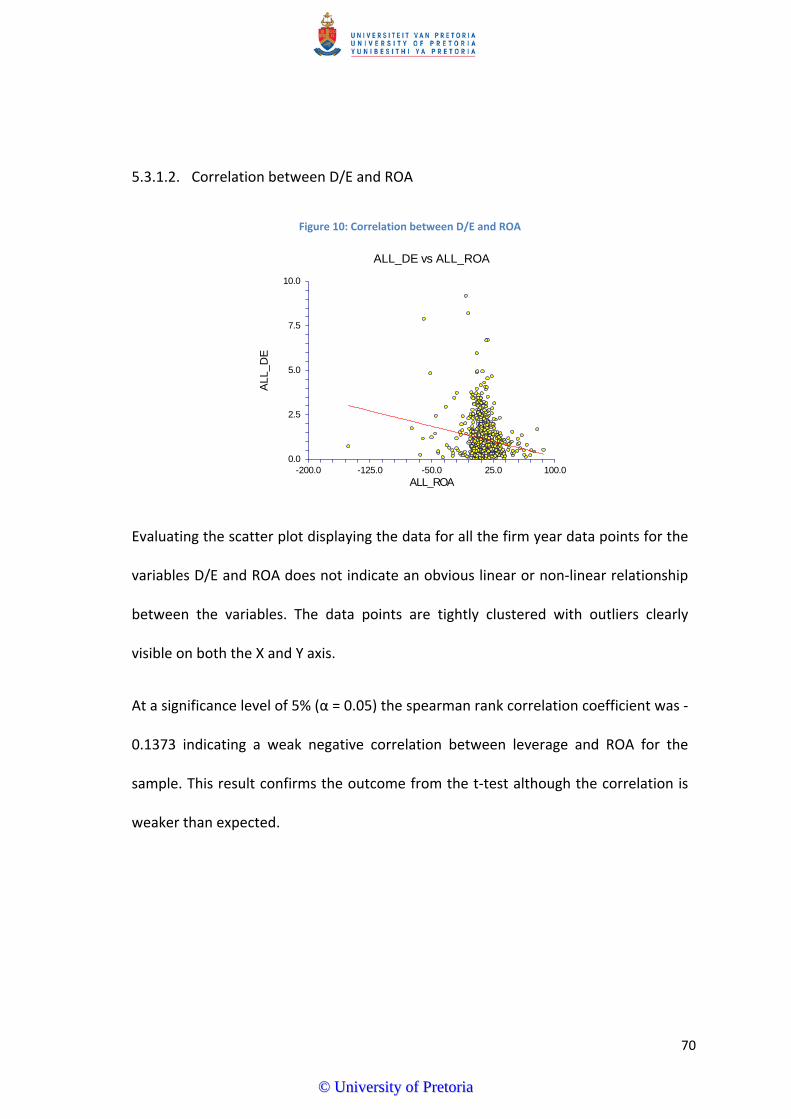
5.3.1.2. Correlation between D/E and ROA

Figure 10: Correlation between D/E and ROA

0.0

2.5

5.0

7.5

10.0

-200.0 -125.0 -50.0 25.0 100.0

ALL_DE vs ALL_ROA

ALL_ROA

ALL

_DE

Evaluating the scatter plot displaying the data for all the firm year data points for the

variables D/E and ROA does not indicate an obvious linear or non‐linear relationship

between the variables. The data points are tightly clustered with outliers clearly

visible on both the X and Y axis.

At a significance level of 5% (α = 0.05) the spearman rank correlation coefficient was ‐

0.1373 indicating a weak negative correlation between leverage and ROA for the

sample. This result confirms the outcome from the t‐test although the correlation is

weaker than expected.

70


5.3.2. Industry median debt levels

The one way analysis of variance (ANOVA) test was executed to determine whether

there was a difference between the median industry debt levels.

Visual inspection of the box plot for the mean industry debt levels (Figure 11) indicate

both unequal variances indicated by the different sizes of the interquartile ranges of

the box plots as well the fact that the data are positively skewed. This can be

witnessed by the large number of positive outliers above the box plots.

The mean and median values also appear to be significantly different based on the

inspection of the industry mean debt level box plot in figure 11. This indicates that

the data is not normally distributed.

71


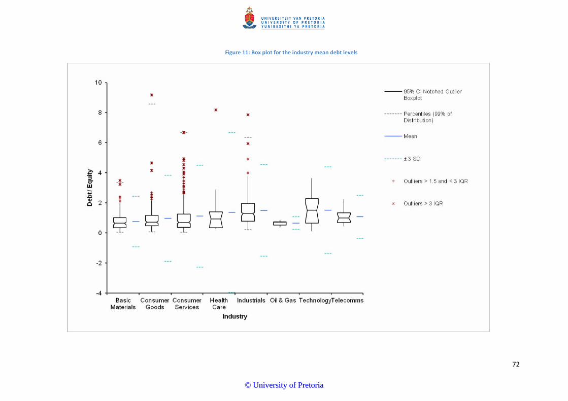
72

Figure 11: Box plot for the industry mean debt levels


73

At a significance level of 5% (α = 0.05) the null hypothesis is rejected and at least two

of the median values have been found to be statistically significantly different from

one another.



Test of Hypothesis two:

All tests for normality were rejected therefore parametric tests for the difference

between means could not be used for this test. The non‐parametric Kruskal‐Wallis

test was therefore used to answer the research hypothesis.

The test of assumptions section of the NCSS output confirms the visual inspection of

the box plots for industry mean debt levels with regards to both equal variances and

the violation of the assumption of normaility.

Table 8: Industry median debt levels test for normality


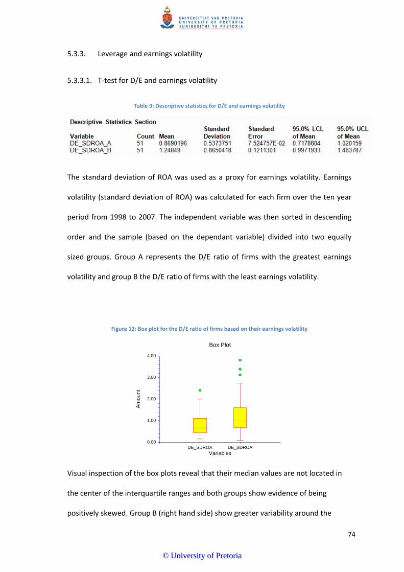
5.3.3. Leverage and earnings volatility

5.3.3.1. T‐test for D/E and earnings volatility

Table 9: Descriptive statistics for D/E and earnings volatility

The standard deviation of ROA was used as a proxy for earnings volatility. Earnings

volatility (standard deviation of ROA) was calculated for each firm over the ten year

period from 1998 to 2007. The independent variable was then sorted in descending

order and the sample (based on the dependant variable) divided into two equally

sized groups. Group A represents the D/E ratio of firms with the greatest earnings

volatility and group B the D/E ratio of firms with the least earnings volatility.

Figure 12: Box plot for the D/E ratio of firms based on their earnings volatility

0.00

1.00

2.00

3.00

4.00

DE_SDROA DE_SDROA

Box Plot

Variables

Am

ount

Visual inspection of the box plots reveal that their median values are not located in

the center of the interquartile ranges and both groups show evidence of being

positively skewed. Group B (right hand side) show greater variability around the

74


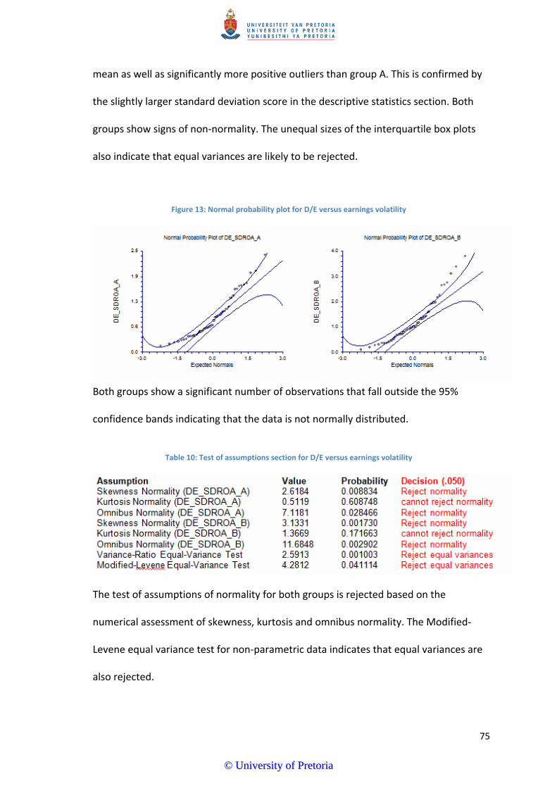
mean as well as significantly more positive outliers than group A. This is confirmed by

the slightly larger standard deviation score in the descriptive statistics section. Both

groups show signs of non‐normality. The unequal sizes of the interquartile box plots

also indicate that equal variances are likely to be rejected.

Figure 13: Normal probability plot for D/E versus earnings volatility

Both groups show a significant number of observations that fall outside the 95%

confidence bands indicating that the data is not normally distributed.

Table 10: Test of assumptions section for D/E versus earnings volatility

The test of assumptions of normality for both groups is rejected based on the

numerical assessment of skewness, kurtosis and omnibus normality. The Modified‐

Levene equal variance test for non‐parametric data indicates that equal variances are

also rejected.

75


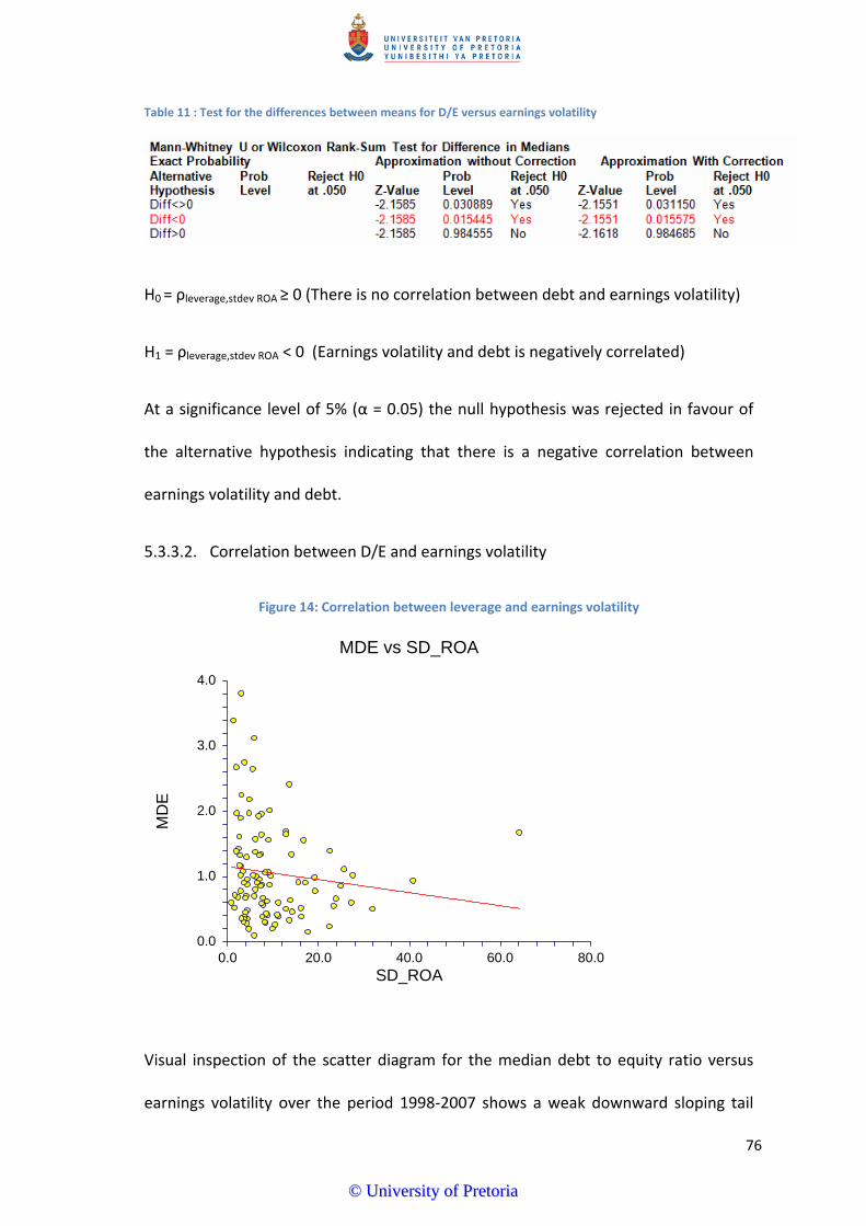
Table 11 : Test for the differences between means for D/E versus earnings volatility



At a significance level of 5% (α = 0.05) the null hypothesis was rejected in favour of

the alternative hypothesis indicating that there is a negative correlation between

earnings volatility and debt.

5.3.3.2. Correlation between D/E and earnings volatility

Figure 14: Correlation between leverage and earnings volatility

0.0

1.0

2.0

3.0

4.0

0.0 20.0 40.0 60.0 80.0

MDE vs SD_ROA

SD_ROA

MD

E

Visual inspection of the scatter diagram for the median debt to equity ratio versus

earnings volatility over the period 1998‐2007 shows a weak downward sloping tail

76


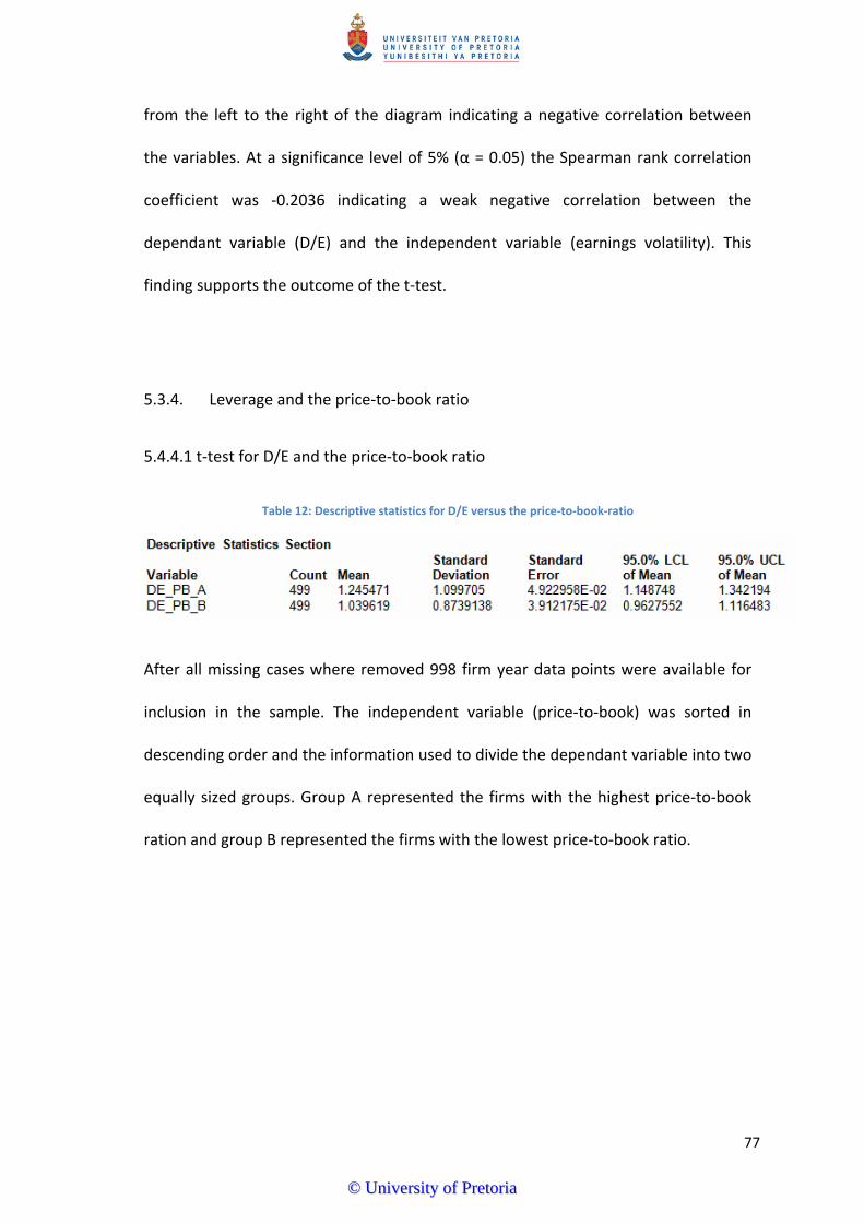
from the left to the right of the diagram indicating a negative correlation between

the variables. At a significance level of 5% (α = 0.05) the Spearman rank correlation

coefficient was ‐0.2036 indicating a weak negative correlation between the

dependant variable (D/E) and the independent variable (earnings volatility). This

finding supports the outcome of the t‐test.

5.3.4. Leverage and the price‐to‐book ratio

5.4.4.1 t‐test for D/E and the price‐to‐book ratio

Table 12: Descriptive statistics for D/E versus the price‐to‐book‐ratio

After all missing cases where removed 998 firm year data points were available for

inclusion in the sample. The independent variable (price‐to‐book) was sorted in

descending order and the information used to divide the dependant variable into two

equally sized groups. Group A represented the firms with the highest price‐to‐book

ration and group B represented the firms with the lowest price‐to‐book ratio.

77


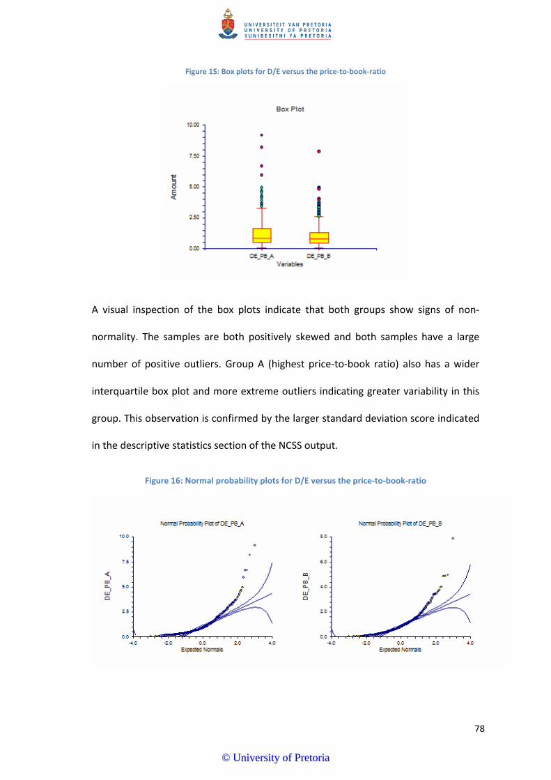
Figure 15: Box plots for D/E versus the price‐to‐book‐ratio

A visual inspection of the box plots indicate that both groups show signs of non‐

normality. The samples are both positively skewed and both samples have a large

number of positive outliers. Group A (highest price‐to‐book ratio) also has a wider

interquartile box plot and more extreme outliers indicating greater variability in this

group. This observation is confirmed by the larger standard deviation score indicated

in the descriptive statistics section of the NCSS output.

Figure 16: Normal probability plots for D/E versus the price‐to‐book‐ratio

78


The normal probability plot indicate that both samples have a large number of firm

year data points that fall outside the 95% confidence bands indicating that the data is

not normally distributed.

Figure 17: Test of assumptions section for D/E versus the price‐to‐book‐ratio

The test of assumptions section of the NCSS data output confirms the visual

inspection of the box and normal probability plots. The assumption of normality in

both samples was rejected based on the numerical calculation of the skewness,

kurtosis and omnibus normality values. The modified‐Levene equal variance test for

non‐parametric data also rejects the assumption of equal variances.

Figure 18: Hypothesis test for D/E versus the price‐to‐book‐ratio



79


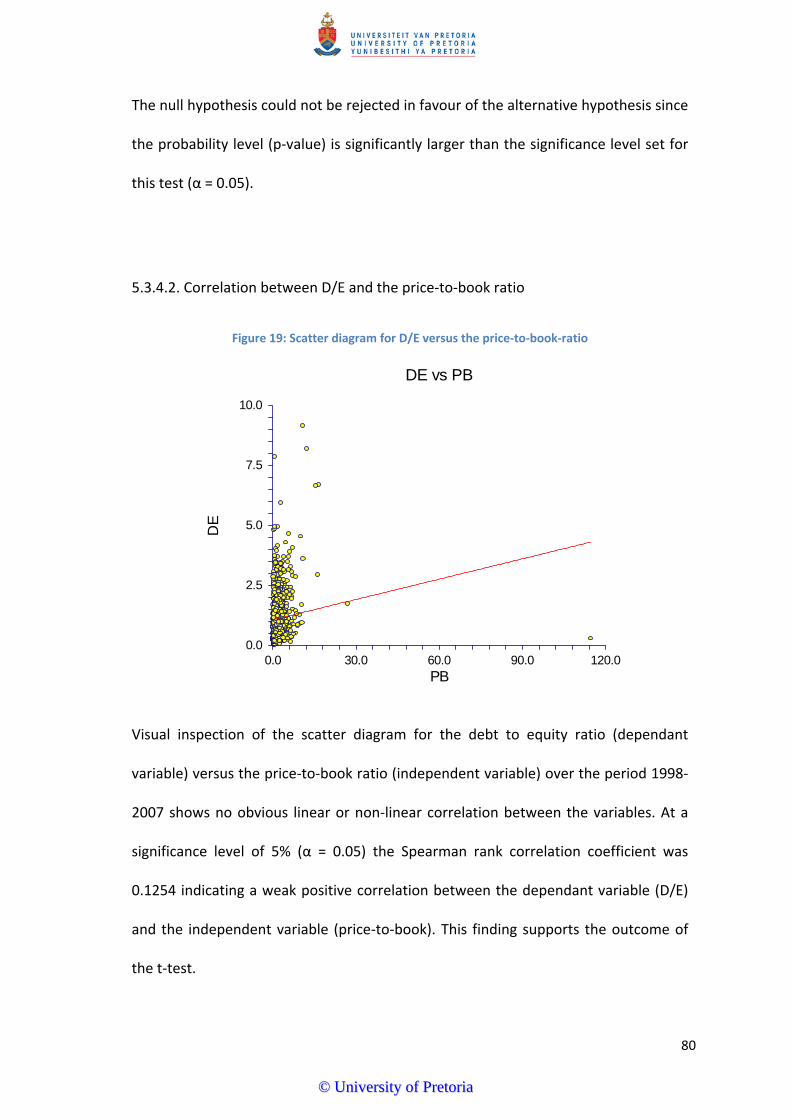
The null hypothesis could not be rejected in favour of the alternative hypothesis since

the probability level (p‐value) is significantly larger than the significance level set for

this test (α = 0.05).

5.3.4.2. Correlation between D/E and the price‐to‐book ratio

Figure 19: Scatter diagram for D/E versus the price‐to‐book‐ratio

0.0

2.5

5.0

7.5

10.0

0.0 30.0 60.0 90.0 120.0

DE vs PB

PB

DE

Visual inspection of the scatter diagram for the debt to equity ratio (dependant

variable) versus the price‐to‐book ratio (independent variable) over the period 1998‐

2007 shows no obvious linear or non‐linear correlation between the variables. At a

significance level of 5% (α = 0.05) the Spearman rank correlation coefficient was

0.1254 indicating a weak positive correlation between the dependant variable (D/E)

and the independent variable (price‐to‐book). This finding supports the outcome of

the t‐test.

80


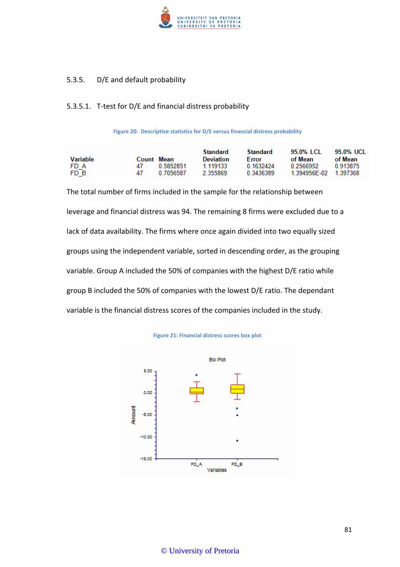
5.3.5. D/E and default probability

5.3.5.1. T‐test for D/E and financial distress probability

Figure 20: Descriptive statistics for D/E versus financial distress probability

The total number of firms included in the sample for the relationship between

leverage and financial distress was 94. The remaining 8 firms were excluded due to a

lack of data availability. The firms where once again divided into two equally sized

groups using the independent variable, sorted in descending order, as the grouping

variable. Group A included the 50% of companies with the highest D/E ratio while

group B included the 50% of companies with the lowest D/E ratio. The dependant

variable is the financial distress scores of the companies included in the study.

Figure 21: Financial distress scores box plot

81


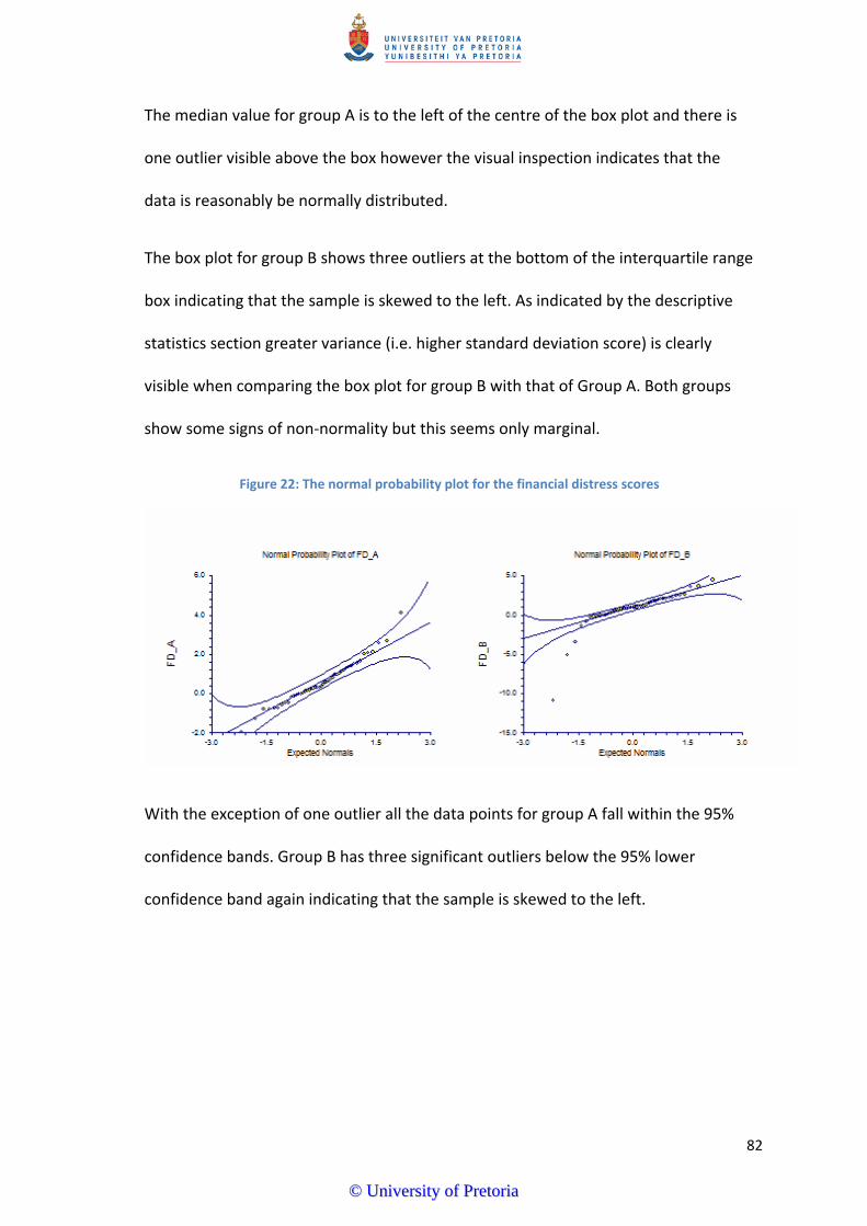
The median value for group A is to the left of the centre of the box plot and there is

one outlier visible above the box however the visual inspection indicates that the

data is reasonably be normally distributed.

The box plot for group B shows three outliers at the bottom of the interquartile range

box indicating that the sample is skewed to the left. As indicated by the descriptive

statistics section greater variance (i.e. higher standard deviation score) is clearly

visible when comparing the box plot for group B with that of Group A. Both groups

show some signs of non‐normality but this seems only marginal.

Figure 22: The normal probability plot for the financial distress scores

With the exception of one outlier all the data points for group A fall within the 95%

confidence bands. Group B has three significant outliers below the 95% lower

confidence band again indicating that the sample is skewed to the left.

82


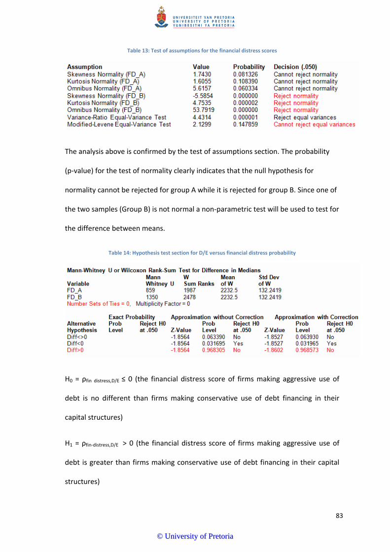
Table 13: Test of assumptions for the financial distress scores

The analysis above is confirmed by the test of assumptions section. The probability

(p‐value) for the test of normality clearly indicates that the null hypothesis for

normality cannot be rejected for group A while it is rejected for group B. Since one of

the two samples (Group B) is not normal a non‐parametric test will be used to test for

the difference between means.

Table 14: Hypothesis test section for D/E versus financial distress probability



capital structures)



structures)

83


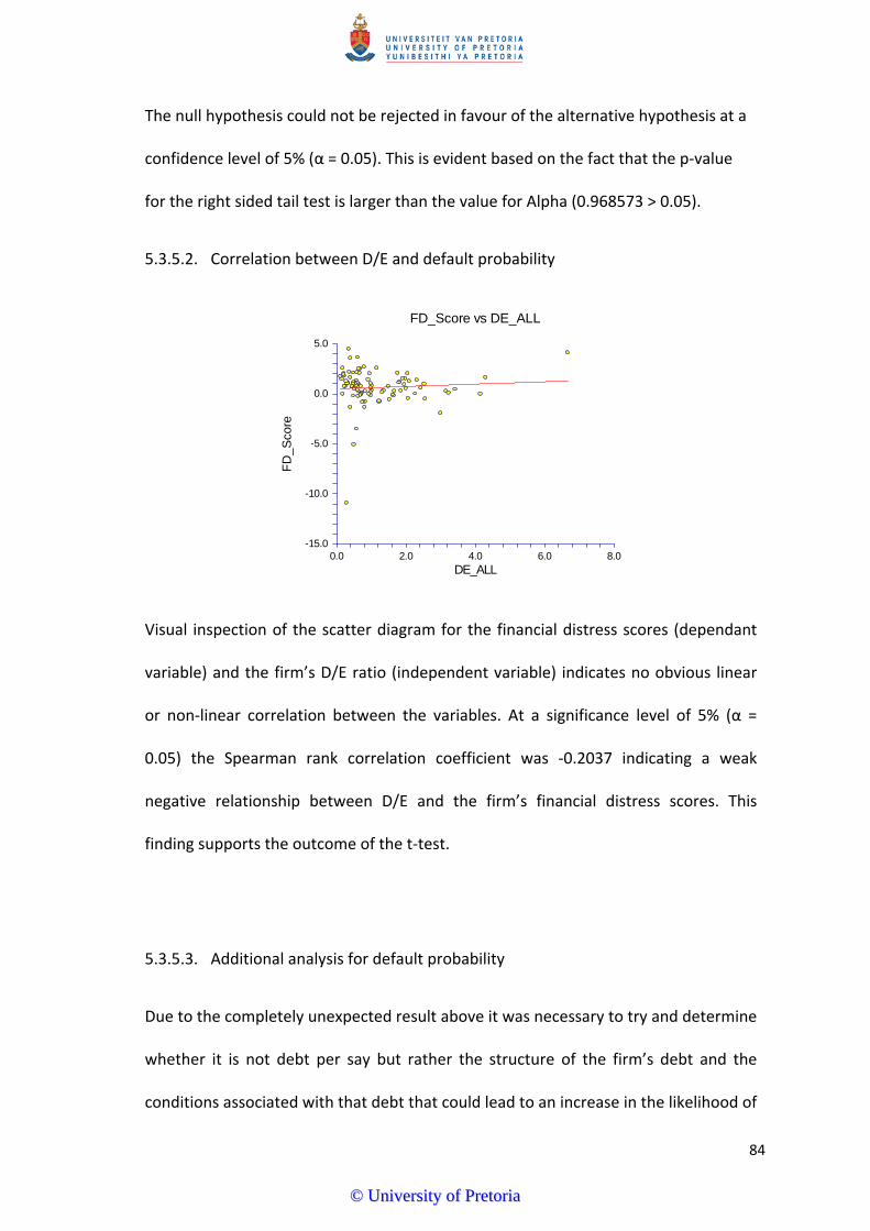
The null hypothesis could not be rejected in favour of the alternative hypothesis at a

confidence level of 5% (α = 0.05). This is evident based on the fact that the p‐value

for the right sided tail test is larger than the value for Alpha (0.968573 > 0.05).

5.3.5.2. Correlation between D/E and default probability

-15.0

-10.0

-5.0

0.0

5.0

0.0 2.0 4.0 6.0 8.0

FD_Score vs DE_ALL

DE_ALL

FD

_Sco

re

Visual inspection of the scatter diagram for the financial distress scores (dependant

variable) and the firm’s D/E ratio (independent variable) indicates no obvious linear

or non‐linear correlation between the variables. At a significance level of 5% (α =

0.05) the Spearman rank correlation coefficient was ‐0.2037 indicating a weak

negative relationship between D/E and the firm’s financial distress scores. This

finding supports the outcome of the t‐test.

5.3.5.3. Additional analysis for default probability

Due to the completely unexpected result above it was necessary to try and determine

whether it is not debt per say but rather the structure of the firm’s debt and the

conditions associated with that debt that could lead to an increase in the likelihood of

84


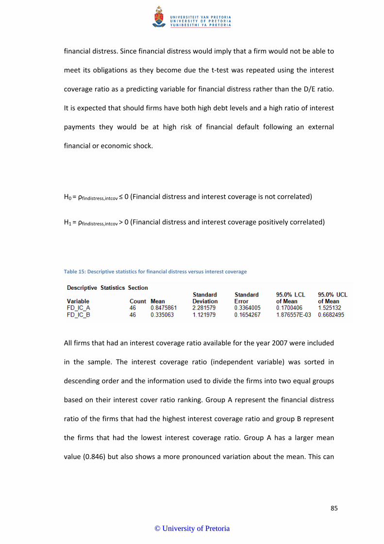
financial distress. Since financial distress would imply that a firm would not be able to

meet its obligations as they become due the t‐test was repeated using the interest

coverage ratio as a predicting variable for financial distress rather than the D/E ratio.

It is expected that should firms have both high debt levels and a high ratio of interest

payments they would be at high risk of financial default following an external

financial or economic shock.

H0 = ρfindistress,intcov ≤ 0 (Financial distress and interest coverage is not correlated)

H1 = ρfindistress,intcov > 0 (Financial distress and interest coverage positively correlated)

Table 15: Descriptive statistics for financial distress versus interest coverage

All firms that had an interest coverage ratio available for the year 2007 were included

in the sample. The interest coverage ratio (independent variable) was sorted in

descending order and the information used to divide the firms into two equal groups

based on their interest cover ratio ranking. Group A represent the financial distress

ratio of the firms that had the highest interest coverage ratio and group B represent

the firms that had the lowest interest coverage ratio. Group A has a larger mean

value (0.846) but also shows a more pronounced variation about the mean. This can

85


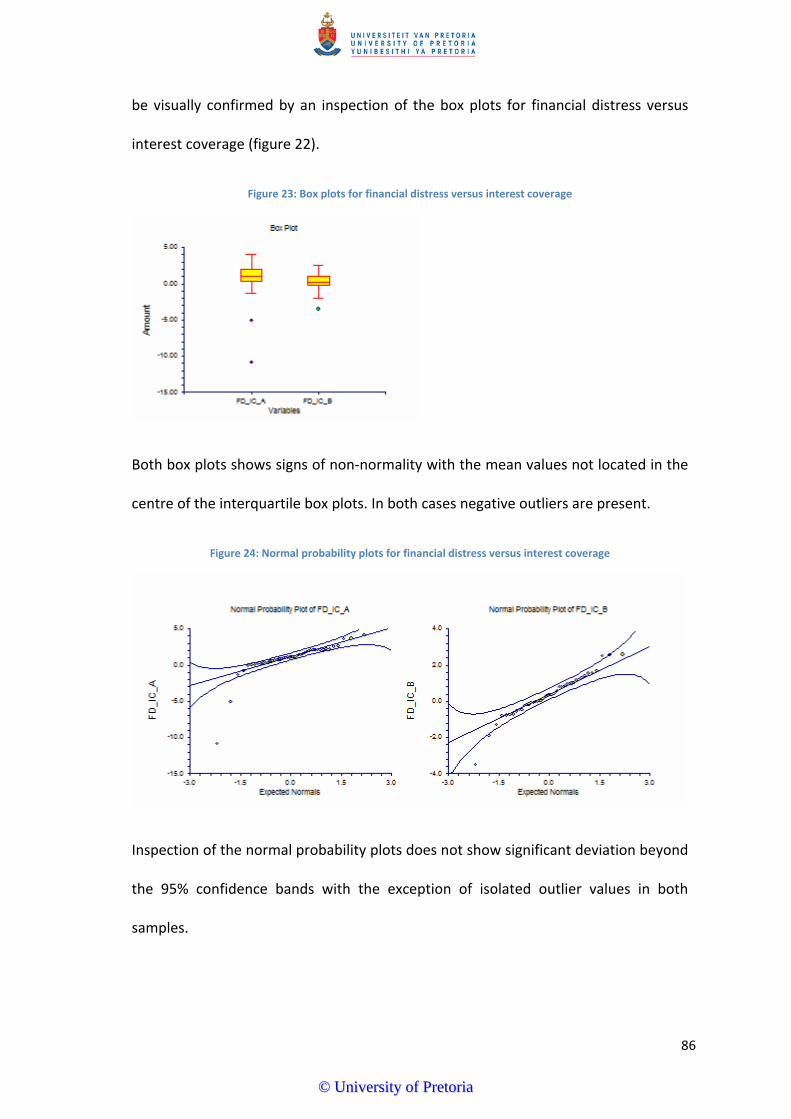
be visually confirmed by an inspection of the box plots for financial distress versus

interest coverage (figure 22).

Figure 23: Box plots for financial distress versus interest coverage

Both box plots shows signs of non‐normality with the mean values not located in the

centre of the interquartile box plots. In both cases negative outliers are present.

Figure 24: Normal probability plots for financial distress versus interest coverage

Inspection of the normal probability plots does not show significant deviation beyond

the 95% confidence bands with the exception of isolated outlier values in both

samples.

86


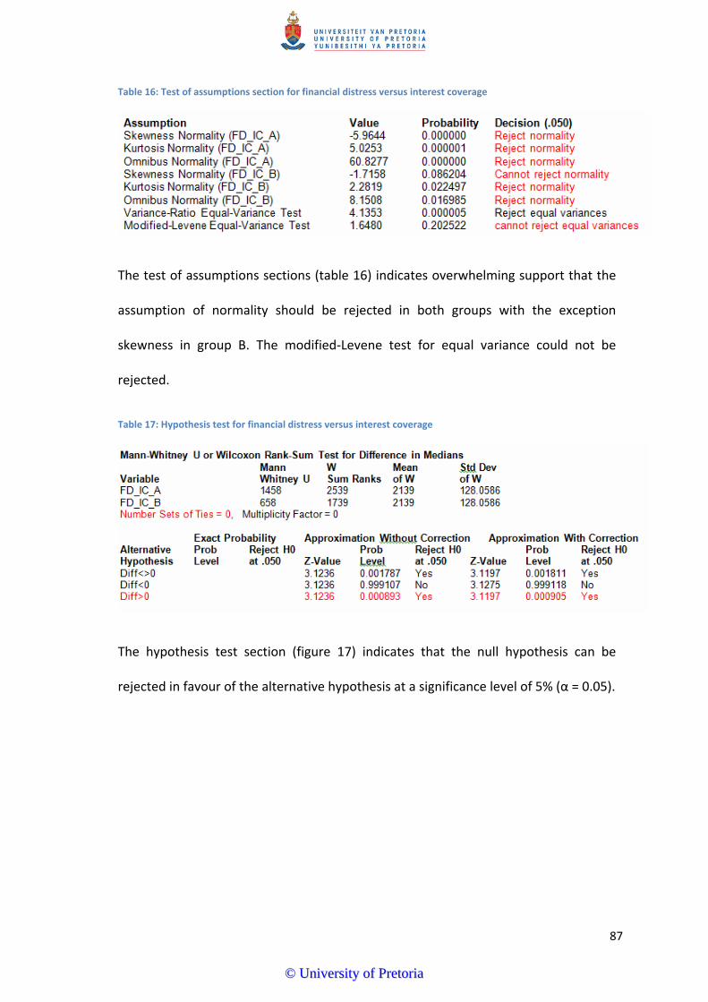
Table 16: Test of assumptions section for financial distress versus interest coverage

The test of assumptions sections (table 16) indicates overwhelming support that the

assumption of normality should be rejected in both groups with the exception

skewness in group B. The modified‐Levene test for equal variance could not be

rejected.

Table 17: Hypothesis test for financial distress versus interest coverage

The hypothesis test section (figure 17) indicates that the null hypothesis can be

rejected in favour of the alternative hypothesis at a significance level of 5% (α = 0.05).

87


6. Chapter Six ‐ Discussion of results

6.1. Introduction

In chapter six the outcome of the statistical of results obtained in chapter five will be

discussed in terms of both the research hypotheses and the literature review in order

to determine whether support is warranted for the aforementioned capital structure

theories and research hypothesis based on the available evidence. Each research

hypothesis will be discussed individually on the basis of the expected outcome of the

hypothesis test, the actual outcome and finally positing potential reasons for the

observed outcomes.

6.2. Discussion of results

6.2.1. Research hypothesis one: the relationship between profitability and debt

The trade‐off theory and the pecking order theory suggest that increased profitability

will have different impacts on the financing decisions of the firm. According to the

trade‐off theory increased profitability will lead to an increase in debt in an effort to

maximise the income tax shield obtained through the tax deductibility of interest

payments. The pecking order theory suggest that firms will prefer to make use of

internal funds over external funds and therefore will require less costly external debt

in times of increased profitability. Similarly firms will prefer to retire costly external

debt in times of good profitability.

88


Research hypothesis 1a:


correlated)


At a significance level of 5% (α = 0.05) the null hypothesis could not be rejected.

Research hypothesis 1b:


correlated)


At a significance level of 5% (α = 0.05) the null hypothesis was rejected in favour of

the alternative hypothesis.

The outcome of the first research hypothesis supports the pecking order theory

which states that there will be a negative correlation between debt and profitability.

This finding is supported by the two sample t‐test which divided the sample data into

two fifty percentile groups based on profitability. The most profitable 50% of firm

year data displayed a lower median debt level (0.69) than the least profitable firm

year data points (1.03). This indicates that the median debt level for the least

profitable 50% of firm year data points is nearly one half greater than that of the 50%

most profitable firm year data points. This result may indicate that firms either use

their profits to retire debt during profitable years, fund projects internally during

profitable years or some combination of both.

89


This outcome is supported by the correlation analysis which indicated a weak

negative correlation between profitably and debt. The correlation was however much

weaker than expected. One potential reason for this may be the fact that there are

significant outliers present in the data that may have skewed the outcome of the

correlation analysis.

Overall the outcome of the T‐test is regarded as much more objective than that of

the correlation analysis and the difference in the median debt levels can be regarded

as both statistically and practically significant since the most profitable firm year data

points indicated nearly 50% less debt than the least profitable firm year data points.

6.2.2. Research hypothesis two: difference between industry median debt levels

According to Frank and Goyal (2010) industry affiliation is a core determinant of firm

specific leverage. Firms that operate in industries that display high median debt levels

will tend to have high levels of debt. Hovakimian, Opler and Titman (2002) site

examples of industries in which the costs associated with debt can be so high that

firms will finance themselves primarily through equity (the bio‐technology and

software industries) whereas firms with low research and development cost, highly

tangible assets and relatively large market capitalisation are expected to have high

debt levels.



90


At a significance level of 5% (α = 0.05) the null hypothesis was rejected indicating that

South African firms also display a significant difference in industry median debt levels.

The technology sector showed the most pronounced levels of debt with the median

firm year debt‐to‐equity ratio being 1.51, more than double that of the basic

materials, consumer goods, consumer services and oil & gas median firm year debt

levels. The underlying factors, such as asset tangibility and research and development

cost, that drives this behaviour did not form a part of this study. The structure,

maturity and type of debt instruments issued, was also not investigated as a part of

this research project. Both of these factors could give significant insight into the

reason for the industry specific debt levels especially when compared to with the

macro‐economic cycle, relative maturity and competitive dynamics in each industry.

This finding offers some support for the optimal capital structure theory.

6.2.3. Research hypothesis three: the relationship between earnings volatility and

debt



The null hypothesis was rejected in favour of the alternative hypothesis.

One of the key factors in deciding on the amount of leverage in a firm’s capital

structure is the firm’s business risk. Business risk can be defined as those factor that

are typically driven by the firms operating strategy, industry dynamics and exposure

91


to economics fluctuations that would include factors such as the interest rate,

changes in commodity prices and the rate of exchange (Opler et al, 1997). Since

South African firms (and the developing economies of the world in general) are in

many instances especially dependant on both commodity prices and the rate of

exchange for both exports and the importation of capital goods it was expected that

earnings volatility would play a major role in the debt financing decisions of South

African firms.

Both the optimal capital structure theory and the pecking order theory predicted that

leverage will decrease as earnings volatility increases.

6.2.4. Research hypothesis four: the relationship between the price‐to‐book ratio

and debt



The null hypothesis could not be rejected in favour of the alternative hypothesis since

the probability level (p‐value) was larger than the specified significance level defined

for the hypothesis test (0.997595 > 0.05.)

The notion that the market value of the firm’s assets less liabilities (net worth) and

leverage is negatively correlated has been expressed by Frank and Goyal (2010) as

reliable capital structure relationship. Booth, Aivazian, Demirguc‐Kunt and

Maksimovic (2001) however question the portability of capital structure theory,

92


especially when concepts are transferred from the developed to the developing

world. One exception they found was that related to the price‐to‐book ratio of firms.

Booth et al (2001) found that the price‐to‐book value varied from trading to a

discount to trading at a premium in different developing countries and therefore the

correlation will vary across countries depending on the accounting principles

adopted. In general the factors that affect capital structure are similar for developed

and developing countries however in the case of business risk and the price‐to book

ratio the signs are often the opposite of what we would expect. One possible reason

might be the fact that firms in developing countries have a greater dependence on

short‐term debt and trade credit (Booth et al, 2001). This view is supported by

Nagesh (2001) who states that long term debt generally constitutes only a small

percentage of total assets, often less than 10% of total assets, probably because few

corporate debt securities are publicly traded in South Africa.

6.2.5. Research hypothesis five: the relationship between debt and the probability

of financial distress



capital structures)



structures)

93


The null hypothesis could not be rejected in favour of the alternative hypothesis.

This result was completely unexpected as logic predicts, and evidence suggest, that

firms with highly leveraged balance sheets would be more susceptible to financial

distress during a period of reduction in the demand for their products or adverse

external financial and economic shocks. This view is supported by Opler et al (1997)

who states that firms with highly leveraged balance sheet are likely to suffer

disproportionately during industry downturns.

The most likely cause for the result is that spurious correlations might have been

formed on the basis of a single aberrant industry or outlier values in more than one

industry. In order to test this theory a second t‐test was run using the interest

coverage ratio as a proxy for leverage as it is assumed that all debt would be interest

bearing. The hypothesis for this test is stated below:

H0 = ρfindistress,intcov = 0 (Financial distress and interest coverage is not correlated)

H1 = ρfindistress,intcov > 0 (Financial distress and interest coverage positively correlated)

In this instance it was possible to reject the null hypothesis in favour of the

alternative hypothesis. Although this does not conclusively answer the question of

whether high levels of debt will lead to a high probability of financial distress it does

point in that direction. It is therefore possible to reasonably deduct that both the

levels and structure (trade creditors and short‐term versus long‐term sources) of debt

plays an important role in the probability of financial default.

It is recommended that this research hypothesis be further unpacked, by industry

and firm, in order to better understand this unexpected result. Specific attention

94


should be paid to industry characteristics, firm level characteristics and the nature of

debt with which the firm is encumbered (i.e. the structure of the debt). The financial

and economic downturn of 2007/8 gives researchers a unique opportunity to further

investigate the relationship between leverage and the probability of financial

distress. Unfortunately due to space and time constraints this goal cannot be

achieved as a part of this research project.

95


7. Chapter seven – Conclusion and recommendations

7.1. Introduction

The concluding chapter of this research report aims to succinctly summarise some of

the main findings and learning that has occurred as a consequence of this process.

The summary of key findings will be followed by recommendations for practitioners

before concluding with suggestions for further research.

7.2. Summary of key findings

It has been said that in some areas theory leads practise and in others theory follows

practise, capital structure research seems to follow practise and still lacks a singular

overarching theory with both goods explanatory and predictive power. It is probably

this shortcoming that has lead researchers like Myers (1984) to conclude that we

know little about how managers make capital structure decisions. One of the

challenges faced by capital structure theory is the fact that the theories are often

diametrically opposed to one another (Barclay & Smith, 1999).

Two possible reasons can be postulated for this: Firstly it has been argued that much

of the empirical research have often been conducted with the specific aim of finding

support for a particular theory thereby biasing the outcome of the research (Frank &

Goyal, 2003) and secondly the practise of capital structure has proven to be a very

contextual matter impacted by the firm, the industry in which the firm operates and

the broader macro‐economic and legal environment (Booth et al, 2001).

96


Despite these challenges there is a belief that progress is being made and that the

continuous interaction between theory and empirical testing will lead to more

sophisticated models able to give corporate finance practitioners better guidance.

One of the challenges that will have to be overcome during this process is the

difficulty of measuring the variables thought to affect capital structure however

researchers will continue to seek and find better proxy variables for key corporate

financing decisions (Barclay & Smith, 1999).

To develop a more thorough understanding of capital structure it is necessary, at

least partially, to break free from the constraints of quantitative research methods in

an effort to learn more from corporate finance practitioners. This view was

championed by Norton (1991) who stated that it is unlikely that capital structure

theory will make any significant progress until such time that greater attention is

placed on the decision making processes of financial managers.

The relationship between leverage and debt was unexpected and are most likely

erroneous. Support for this argument can be found in the fact that the correlation

between the interest coverage ratio of firms and their financial distress probability is

positively correlated. This result may have been caused by a single industry skewing

the overall result of the test or alternatively by a number of outliers present in the

data across industries. There is without doubt also some element of bias in the data

as all firms with a D/E ratio greater than 10 where excluded from the sample. Several

firms reported D/E ratios of several hundred to one and including these in the sample

would have contaminated the efforts of the research project.

97


The positive relationship between the price‐to‐book ratio and leverage was also

surprising as it is often believed that the South African financial and capital markets

exhibit characteristics more like that of the developed rather than the developing

world. One potential reason for this might be the fact that South Africa has a highly

developed stock market, comparable to that of the Western world, but our debt

market is still relatively under traded. This gives rise to the fact that South African

listed firms have relatively low long term debt to net asset ratios.

As expected earnings volatility and leverage was negatively correlated. This factor

suggests that firms that earn most of their revenue through either imports or exports

are subjected to the vicissitudes of the Rand as well as the commodity price cycles

are likely to exhibit chronically lower debt levels than firms that operate more

domestically. Those Firms’ dependant on imported capital machinery can of course

always time the purchase of capital goods to coincide with favourable exchange rate

conditions but this would offer limited shelter at best.

Finally, since this research project has found support for both the optimal capital

structure theory and the pecking order theory the outcome concurs with the findings

of Myers (2002) that capital structure theories are conditional, not general, and are

at best dependent on firm, industry and country specific factors.

98


7.3. Recommendations

7.3.1. Recommendations for practitioners

Capital structure theory is a developing area of corporate finance and as such has

very few general prescriptions it can offer to practitioners, however the following

guidelines does offer valuable insight:

I. Firms should match their leverage levels with their earnings volatility. Firms with

greater earnings volatility should use less leverage in their capital structures than

firms with relatively stable earnings.

II. To the extent that earnings are mean reverting firms can increase their leverage.

III. The commonly expressed notion that South African firms are underleveraged should

be viewed with at least some scepticism. The Asian crisis showed that the difference

in leverage between firms that became financially distressed and those that

remained financially sound were very small. Individual operating characteristics seem

to matter at least as much as capital structure and market and economic conditions.

IV. There is some evidence that South African firms underutilise long term debt in their

capital structures. Changing the structure of debt can have potentially beneficial

effect on the firms risk profile and cost of capital.

99


7.3.2. Recommendations for researchers

I. Continuing to seek empirical evidence in support of existing capital structure theories

has reached a point of diminishing returns. These theories offer at best conditional

explanatory and predictive power and cannot be transferred across firms, industries

and countries without encountering some serious caveats. Some combination of

qualitative and quantitative research probably offers the greatest probability of

progress. The fact that capital structure theory has so little practical value to offer

practitioners should be an indication that this area of research is ready for disruptive

rather than evolutionary thinking.

7.4. Suggestions for further research

Capital structure theory offer rich opportunities for further research. There are

numerous methods in which this research can be advanced further as well as some

additional suggestions based on experiences gained during the completion of this

research report:

i. This study made use of quantitative data in an effort to explain the observed capital

structures of firms over the 1998‐2007 time period. Norton (1991) indicated that

there are limitations associated with using empirical data to determine which factors

account for the capital structure decisions that managers of firms make. One way to

overcome this problem would be to adopt a qualitative or survey based approach in

order to ask managers/practitioners what factors affect the way in which they

structure the capital structures of their firms rather than to use proxy variables and

100


ii. The relationship between economic variables and the observed capital structure of

firms could potentially offer significant insight into the behaviour of South African

firms. The major macro‐economic variables; gross domestic product, consumer

inflation rate, production inflation rate, the prime interest and repo rates and

exchange rates immediately come to mind. The motivation for such a study would be

an effort to understand how the macro‐economic environment affects the earnings

volatility and capital structure of firms. It will be of particular importance to gain

insight into how the behaviour of exchange rate dependant firms (importers and

resellers and those firms dependent on exports for the majority of their revenues)

are impacted versus firms that source and sell locally and are consequently

somewhat less affected by the vicissitudes of the South African Rand.

101


iii. The relationship between observed leverage levels and the probability of financial

distress warrants further investigation, especially in the light of the recurring

statement that South African firms are under leveraged. The 2007/8 financial crisis is

the perfect backdrop for such research to take place as it allows researchers a unique

opportunity to evaluate the impact of external financial and economic shocks on

firms with heterogeneous capital structures.

iv. Most studies of capital structure in South Africa are driven by data availability which

bias them toward large and mature firms listed on the main board of the

Johannesburg Stock Exchange. In order to better understand the capital market

frictions experienced by smaller firms early in their life cycles it would be meaningful

to conduct capital structure research on companies listed on the Alternative

Exchange (Alt‐X) of the Johannesburg Stock Exchange. Given the desperate need for

entrepreneurship and the fact that most small enterprises in South Africa are under

capitalised this area of capital structure research might prove especially meaningful

from both a theoretical and practical perspective.

7.5. Conclusion

Since the introduction of Modigliani and Miller’s capital structure irrelevance

proposition the subject of how and why firms choose a specific capital structure have

remained a controversial topic (Myers, 1984). Unfortunately it would seem that the

capital structure literature of the past five decades has not been able to emulate the

success that corporate finance research have been able to achieve in the area of

102


capital budgeting (Graham & Harvey, 2002) and therefore practitioners have been

left with a set of heuristics or rules of thumb to make decisions about their choices of

debt, equity and other hybrid financing instruments (Myers, 2001). Researchers like

Barclay and Smith (1999) do however indicate that significant strides are being made

in the quality of the empirical studies being conducted in the area of capital structure

research.

Much of the debate to date have centred around the argument of debt versus equity

in the observed capital structure of firms but in addition to explaining the basic

leverage choice (i.e. how much debt a company should use) Barclay and Smith (1999)

states that useful capital structure theories should address issues such as the

structure of debt (i.e. debt maturity, options and debt covenants etc.). According to

Barclay and Smith (1999) companies don’t only choose a level of leverage but rather

they decide on a coherent package of financial policies and instruments. Under such

conditions it is foreseeable that the context of the firm will become even more

important in explaining existing leverage choices in an effort to offer meaningful

guidance for future policy decisions. The target debt‐to‐equity ratio should include

factors such as the company’s projected investment requirements; the level and

stability of its operating cash flows; its tax status; the possible loss of value should the

company be unable to make positive net present value investments or be forced into

financial distress and the ability to raise capital on short notice without excessive

ownership dilution.

In the South African context this equates to significant research opportunities and

increased collaboration between practitioners and academia.

103


8. References

Albright, S.C., Winston, W.L. & Zappe, C.J. (2006) Data analysis and decision making

with Microsoft Excel. United States of America: Thomson South‐Western.

Arrif, M., Hassan, T. & Shamsher, M. (2008) How capital structure adjust dynamically

during financial crises. Corporate finance review. 13(3), 11‐24.

Baker, M. & Wurgler, J. (2002) Market timing and capital structure. The journal of

finance. 57(1), 1‐32.

Barclay, M.J. & Smith, C.W. (1999) The capital structure puzzle: another look at the

evidence. Journal of applied corporate finance. 12(1), 8‐20.

BBC News (2010) Timeline: the credit crunch to downturn. Retrieved from the BBC

News website: http://news.bbc.co.uk/2/hi/7521250.stm (accessed 21/09/10).

Bodie, Z., Kane, A. & Marcus, J. (2009) Investments, 8th edition. New York: McGraw

Hill.

Booth, L., Aivazian, V., Demirgruc‐Kunt, A. & Maksimovic, V. (2001) Capital structures

in developing countries. The journal of finance. 56(1), 87‐130.

Bowen, R.M., Daley, L.A. & Huber, C.C. (1982) Evidence on the existence and

determinants of inter‐industry differences in leverage. Financial management. 11(4),

10‐20.

Brounen, D., De Jong, A. & Koedijk, K. (2004) Corporate finance in Europe:

confronting theory with practise. Financial management. 33(4), 71‐101.

104


http://news.bbc.co.uk/2/hi/7521250.stm

Cai, F. & Ghosh, A. (2003) Test of capital structure theory: A binomial approach.

Journal of business and economic studies. 9(2), 20‐32.

Cameron, S. & Price, D. (2009) Business research methods: a practical approach.

London: Chartered institute of personnel development.

Correia, C. & Cramer, P. (2008) An analysis of cost of capital, capital structure and

capital budgeting practises: a survey of South African listed companies. Meditari

accountancy research. 16(2), 31‐52.

De Angelo, H., De Angelo, L. & Stulz, R.M. (2010) Seasoned equity offerings, market

timing, and the corporate lifecycle. Journal of financial economics. 2010(95), 275‐295.

Fama, F.E. & French, K.R. (2005) Financing decisions: who issues stock? Journal of

financial economics. 76, 549‐582.

Firer, C., Ross, S.A., Westerfield, R.W. & Jordan, B.D. (2008) Fundamentals of

corporate finance: 4th South African edition. Berkshire: McGraw Hill.

Frank, M.Z. & Goyal, V.K. (2003) Testing the pecking order theory of capital structure.

Journal of financial economics. 67, 217‐248.

Gitman, L.J. (2003) Principles of managerial finance. Boston: Addison

Wesley/Pearsons education.

Graham, J. & Harvey, C. (2001) The theory and practise of corporate finance. Journal

of financial economics. 60, 187‐243.

Graham, J. & Harvey, C. (2002) How do CFOs make capital budgeting and capital

structure decisions? Journal of applied corporate finance. (15(1), 8‐23.

105


Gropp, R. & Heider, F. (2009) The determinants of bank capital structure. European

central bank working paper series. 1096, 1‐50.

Hovakimian, A., Opler, T. & Titman, S. (2002) The capital structure choice: new

evidence for a dynamic tradeoff model. Journal of applied corporate finance. 15(1),

24‐30.

Leary, M.T. & Roberts, M.R. (2010) The pecking order, debt capacity, and information

asymmetry. Journal of financial economics. 95, 332‐355.

Lewellen, K. (2006) Financing decisions when managers are risk averse. Journal of

financial economics. 82, 551‐589.

Myers, S.C. (1984) The capital structure puzzle. The journal of finance. 39(3), 575‐589.

Myers, S.C. (2002) Financing of corporations. Handbook of the economics of finance.

Negash, M. (2001) Debt, tax shield and bankruptcy cost: evidence from the JSE.

Investment analyst journal. 54, 33‐44.

Opler, T.C., Saron, M. & Titman, S. (1997) Designing capital structure to create

shareholder value. Journal of applied corporate finance. 10(1), 21‐32.

Ovtchinnikov, A.V. (2010) Capital structure decisions: evidence from deregulated

industries. Journal of financial economics. 95, 249‐274.

Pallant, J. (2007) SPSS survival manual. Berkshire: McGraw Hill/Open university press.

106


107

Rayan, K. (2008) Financial leverage and firm value. Master’s degree of Business

Administration Dissertation, University of Pretoria: Gordon Institute of business

Science.

Ryen, G.T., Vasconcellos, G.M. & Kish, R.J. (1997) Capital structure decisions: what

have we learned. Business horizons. September‐October, 41‐50.

Salkind, N.J. (2007) Statistics for people who think they hate statistics. California:

SAGE publications.

Shivdasani, A. & Zenner, M. (2005) How to choose a capital structure: navigating the

debt‐equity decision. Journal of applied corporate finance. 17(1), 26‐35.

Titman, S. & Wessels, R. (1988) The determinants of capital structure choice. The

journal of finance. 43(1), 1‐19.

Ward, M. & Price, A. (2008) Turning vision into value: Corporate finance for non‐

financial executives. Pretoria: Van Schaik Publishers.

Yaffee, R. (2003). A primer for panel data analysis [internet]. Connect information

technology at NYU, fall edition. Available from

http://www.nyu.edu/its/pubs/connect/fall03/yaffee_primer.html (accessed

30/10/2010).

Zaher, T.S. (2010) Performance of debt free firms. Managerial finance, 36(6), 491‐

501.

Zikmund, W.G. (2003) Business research methods, 7th edition. Ohio: Thomson South

Western.


http://www.nyu.edu/its/pubs/connect/fall03/yaffee_primer.html

Documents

Capital structure: profitability, earnings volatility and