Embed Size (px)
Citation preview
Capsule Deep Generative ModelThat Forms Parse Trees
Yifeng LiDepartment of Computer Science
Brock UniversitySt. Catharines, Canada
Xiaodan ZhuDepartment of Electrical and Computer Engineering
Queen’s UniversityKingston, Canada
Richard NaudBrain and Mind Research Institute
University of OttawaOttawa, Canada
Pengcheng XiDigital Technologies Research Centre
National Research Council CanadaOttawa, Canada
Abstract—Supervised capsule networks are theoretically ad-vantageous over convolutional neural networks, because they aimto model a range of transformations of local physical or abstractobjects and part-whole relationships among them. However, itremains unclear how to use the concept of capsules in deepgenerative models. In this study, to address this challenge, wepresent a statistical modelling of capsules in deep generativemodels where distributions are formulated in the exponentialfamily. The major contribution of this unsupervised method isthat parse trees as representations of part-whole relationshipscan be dynamically learned from the data.
Index Terms—deep learning, generative model, capsule net,parse tree, exponential family
I. INTRODUCTION
Deep neural networks and learning algorithms haveachieved grand successes in a variety of areas where data arecomplicated and plenty [1]–[3]. Behind these achievements,the spirit is distributed representation learning [4], which says,any discrete object, symbols or sequence in our world can berepresented by a vector of continuous values. This philosophyis strongly supported by its modern implementations in naturallanguage processing through word embedding [5], [6], andcomputer vision through convolutional neural networks [7],[8].
However, distributed representation does not mean thatstructured latent representations are not important in neuralnetworks. Actually, it is an open and foundational question.At least, the huge adoption of convolutions in various typesof data beyond images indicates that sophisticated structuresoften help achieve state of the art performance. A commonstruggle that current supervised and unsupervised neural net-works are facing is that complicated symbolic manipulationsand reasonable combinations of local patterns can not bewell handled. The introduction of capsule networks stirs newthoughts on how local parts are learned and combined to
This research is supported by the New Beginning Ideation Fund from theNational Research Council Canada.
form a cohesive role, and how features are disentangled withincapsules. In the supervised setting, a capsule is a set of neuralunits that are activated or depressed together [9], [10]. Whilea single unit is barely useful in representing comprehensiveinformation, a set of units is. The introduction of capsulesgoes far beyond an improvement of convolutions. It advocatesa family of models that carves the flow of information withinneural networks. Interestingly, the dynamic routing of capsulesin these deterministic capsule networks are realized usinggenerative techniques such as expectation maximization (EM)[10], because it is in fact an inference problem. This naturallyinspires the studies of capsules in generative models. Inthe simplest case, exponential family restricted Boltzmannmachine (exp-RBM) and Helmholtz machine (exp-HM) areextended to capsule RBM (cap-RBM) and HM (cap-HM)by replacing unit latent variables with stochastic capsules[11]. Although capsules in these models can be contextuallyactivated, part-whole trees, i.e. parse trees, are not formed inthe latent space.
To push forward the front line of research in this direction,we propose a new exponential family deep generative modelin this paper to automatically and dynamically build parsetree among stochastic capsules for a given sample. The paperis organized as follows. Insights into closely related workis provided in Section II. The proposed model and learningrules are described in Section III. Preliminary experiments arereported in Section IV, followed by a discussion (V).
II. RELATED WORK
A. Transforming Auto-Encoder
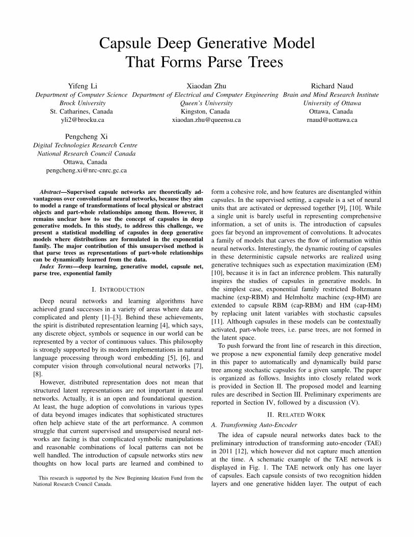
The idea of capsule neural networks dates back to thepreliminary introduction of transforming auto-encoder (TAE)in 2011 [12], which however did not capture much attentionat the time. A schematic example of the TAE network isdisplayed in Fig. 1. The TAE network only has one layerof capsules. Each capsule consists of two recognition hiddenlayers and one generative hidden layer. The output of each
recognition component is a 3 by 3 pose matrix M , and anactivation probability a. The pose matrix is then multiplied bythe affine or 3D transformation matrix W . The transformedmatrix is then fed into the generative component to produce apatch within an reconstructed image. The patch is multipliedby the activation probability a. A pose matrix or vectormay potentially represent any properties of a visual entity.A vote matrix is transformed from the pose matrix. TAEcan be viewed as a prototype of generative-like architecturewith capsules for image generation. However, the 3 by 3transformation matrix is not learned from data, but instead ispredefined when making the input-output pair of each trainingimage. Thus, the real application of TAE is very limited.
Pose Matrix
11x11
96
9611x11
32 units
64 units
128 units
22x22
96
96
22x22
32 units
64 units
128 units
a1M 1
V 1(M 1W 1)
a2M 2
V 2 (M 2W 2)
Input Image
Reconstructed Image
RecognitionUnits
GenerativeUnits
ActivationProbability
Vote Matrix
Capsule
Fig. 1: Example of transforming autoencoder presented in [12].
B. Vector Capsule Net
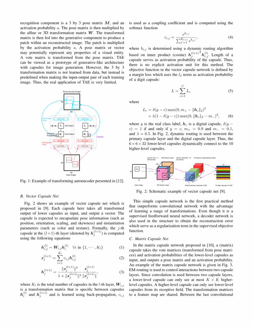
Fig. 2 shows an example of vector capsule net which isproposed in [9]. Each capsule here takes all transformedoutput of lower capsules as input, and output a vector. Thecapsule is expected to encapsulate pose information (such asposition, orientation, scaling, and skewness) and instantiationparameters (such as color and texture). Formally, the j-thcapsule at the (l+1)-th layer (denoted by h(l+1)
j ) is computedusing the following equations
h(l)i,j = Wi,jh
(l)i ∀i in {1, · · · ,Kl} (1)
s(l+1)j =
Kl∑i=1
ci,jh(l)i,j (2)
h(l+1)j =
‖s(l+1)j ‖2
1 + ‖s(l+1)j ‖2
s(l+1)j
‖s(l+1)j ‖
, (3)
where Kl is the total number of capsules in the l-th layer,Wi,j
is a transformation matrix that is specific between capsulesh(l)i and h(l+1)
j and is learned using back-propagation, ci,j
is used as a coupling coefficient and is computed using thesoftmax function
ci,j =ebi,j∑Kl+1
j′=1 ebij′
, (4)
where bi,j is determined using a dynamic routing algorithm
based on inner product (cosine) h(l+1)j
Th(l)i,j . Length of a
capsule serves as activation probability of the capsule. Thus,there is no explicit activation unit for this method. Theobjective function in the vector capsule network is defined bya margin loss which uses the l2 norm as activation probabilityof a digit capsule:
L =
C∑c=1
Lc (5)
where
Lc = δ(y − c) max(0,m+ − ‖hc‖2)2
+ λ(1− δ(y − c)) max(0, ‖hc‖2 −m−)2, (6)
where y is the real class label, hc is a digital capsule, δ(y −c) = 1 if and only if y = c, m+ = 0.9 and m− = 0.1,and λ = 0.5. In Fig. 2, dynamic routing is used between theprimary capsule layer and the digital capsule layer. Thus, the6×6×32 lower-level capsules dynamically connect to the 10higher-level capsules.
Kernel: 9x9 -> 1256 kernels
256 feature maps
Kernel: 9x9x256 -> 832 kernels
32 feature maps/capsule types
6x6x32 primary capsules of 8D
6
6
8
20
20
256
9x9
9x9
A cap
sule
of 8
D
32
28
28
10 digit capsules of 16DInput image
256 feature maps
10
16
Fig. 2: Schematic example of vector capsule net [9].
This simple capsule network is the first practical methodthat outperforms convolutional network with the advantageof learning a range of transformations. Even though it is asupervised feedforward neural network, a decoder network isalso used in the structure to obtain the reconstruction errorwhich serve as a regularization term in the supervised objectivefunction.
C. Matrix Capsule Net
In the matrix capsule network proposed in [10], a (matrix)capsule takes the vote matrices (transformed from pose matri-ces) and activation probabilities of the lower-level capsules asinput, and outputs a pose matrix and an activation probability.An example of the matrix capsule network is given in Fig. 3.EM-routing is used to control interactions between two capsulelayers. Since convolution is used between two capsule layers,a lower-level capsule can only see at most K × K higher-level capsules. A higher-level capsule can only see lower-levelcapsules from its receptive field. The transformation matricesto a feature map are shared. Between the last convolutional

capsule layer and class capsules, a class capsule can see alllower-level capsules. Transformation matrices from the samefeature map are shared to the class capsules.
5x5
32
32
Input image
14 14 6 4 32
5x5 params per kerneltotal: 5x5xA params this layer
Convolutional Layer 1
A B C D
E
Ax(4x4+1) params per kerneltotal: Ax(4x4+1)xB params this layer
KxKxBx4x4 params per kerneltotal: KxKxBx4x4xC params this layer
KxKxBx4x4 params per kerneltotal: KxKxBx4x4xC params this layer
total: Dx4x4xC params this layer
Primary Capsule Layer Convolutional Capsule Layer 1
Convolutional Capsule Layer 2
Class Capsules
14 6414
KxK
KxK
Fig. 3: Schematic example of matrix capsule net [10].
Suppose capsule Cj is the j-th capsule in the l+1 layer, andcapsule Ci is the i-th capsule in the l-th layer. The connectionsfrom Ci to Cj is represented by transformation matrix Wij ,which transforms the pose matrix Hi to vote matrix Vij usingVij = HiWij . Each capsule has two bias parameters: βa andβu, which combine with the vote matrices from the lower-level capsules to determine the activation probability of thecapsule. The biases βa and βu can be respectively the samefor all capsules. This process is visualized in Fig. 4. Thus,the parameters of a capsule network include transformationmatrices on the connections and biases on the capsules.
H 1( l) H 2
( l) H 3( l) H 4
( l) H 5( l)
W 2,2(l+1)W 1,2
(l+1) W 4,2(l+1)W 3,2
(l+1) W 5,2(l+1)
a1(l) a2
(l) a3(l) a4
(l) a5(l)
βu βa
H 2( l+1) a2
(l+1)
C1(l) C 2
(l) C 3(l) C 4
(l) C5(l)
C 2(l+1)
V 1,2(l) V 2,2
(l) V 3,2(l) V 4,2
(l) V 5,2(l)
C1(l+1) C 3
(l+1)
Fig. 4: Input and output of a matrix capsule. Each noderepresents a matrix capsule.
A capsule network is composed of multiple capsule layers.The outputs of capsules in layer l + 1 is based on the outputof capsules in layer l. The model parameters are learned usingback-propagation. A cost function is defined by comparing theactual class label with the activations of the class capsules. Thespread loss function used in [10] is defined as
L =
C∑c=1,c 6=t
(max
(0,m− (at − ac)
))2, (7)
where at is the activation of the capsule corresponding to theactual class t, ac’s are activations of other classes, and m isa margin which increases from 0.2 to 0.9. Cross-entropy losscan also be used even though
∑Cc=1 ac 6= 1. To build the part-
whole relationship among capsules, EM routing is proposedto dynamically activate parent capsules.
D. Generative Capsule Nets
The statistical modelling of capsules has been exploredbased on the exponential family RBMs and HMs [13]–[15].The main idea of the capsule RBM (cap-RBM) proposed in[11] is to replace individual latent variables with stochastic
capsules, each of which is composed of a vector (hk) of hiddenrandom variables following exponential family distributions,and a Bernoulli variable (zk) as activity indicator of thecapsule. An example of such network is displayed in Fig. 5a.Assume the vector of variables x has M units, and the hiddenlayer has K capsules, each of which has J variables and oneswitch variable. The base distributions of capsule RBM aredefined in natural form of exponential family as
p(x) =
M∏m=1
exp(aTmsm + log f(xm)−A(am)
)(8)
p(h) =
K∏k=1
J∏j=1
exp(bTk,jtk,j + log g(hk,j)−B(bk,j)
)(9)
p(z) =
K∏k=1
exp(ckzk − C(zk)
), (10)
The joint distribution is formulated as an energy-based dis-tribution: p(x,h, z) = 1
Z exp(− E(x,h, z)
), where Z is
the partition function, and E(x,h, z) is the energy functiondefined as
E(x,h, z) =−M∑
m=1
(aTmsm + log f(xm)
)−
K∑k=1
J∑j=1
(bTk,jtk,j + log g(hk,j)
)− cTz
−K∑
k=1
zk(xTWkhk). (11)
Inheriting the decomposibility of exp-RBMs, the condition-als of cap-RBM can be obtained in natural forms:
p(x|h, z) =
M∏m=1
p(xm|η(am)
), (12)
p(h|x, z) =
K∏k=1
J∏j=1
p(hk,j |η(bk,j)
), (13)
p(z|x,h) =
K∏k=1
BE(zk|η(ck)
), (14)
where function η(·) maps the natural posterior parameters tothe standard forms.
One advantage of cap-RBM is that the activity of capsulesare dynamically inferred. Different samples activate differentsubset of capsules. Innovation is required to generalize theconcept of cap-RBM to deep generative models. Capsule HM(cap-HM) is the most straightforward generalization of cap-RBM for directed multi-layer capsule models. In cap-HM, thejoint distribution of visible variables and L layers of latentvectors is factorized as:
p(x,h, z) =p(x|h(1), z(1))( L−1∏
l=1
p(h(l), z(l)|h(l+1), z(l+1)))
p(h(L), z(L)). (15)
x
h1, z1 h2, z2 h3, z3 h4, z4
W 1 W 2 W 3 W 4
a
b1,c1 b2,c2 b3,c3 b4,c4
(a) Capsule RBM.
x
h1(1) , z1
(1) h2(1) , z2
(1) h3(1) , z3
(1) h4(1) , z4
(1)
W 1(1) W 2
(1) W 3(1) W 4
(1)
a
b1(1) ,c1
(1) b2(1) ,c2
(1) b3(1) ,c3
(1) b4(1) ,c 4
(1)
h1(2) , z1
(2) h2(2) , z2
(2) h3(2) , z3
(2) h4(2) , z4
(2)
W 1 :4,1(2) W 1 :4,2
(2) W 1 :4,3(2) W 1 :4,4
(2)
b1(2) , c1
(2) b2(2) , c2
(2) b3(2) , c3
(2) b4(2) , c4
(2)
(b) Capsule HM.
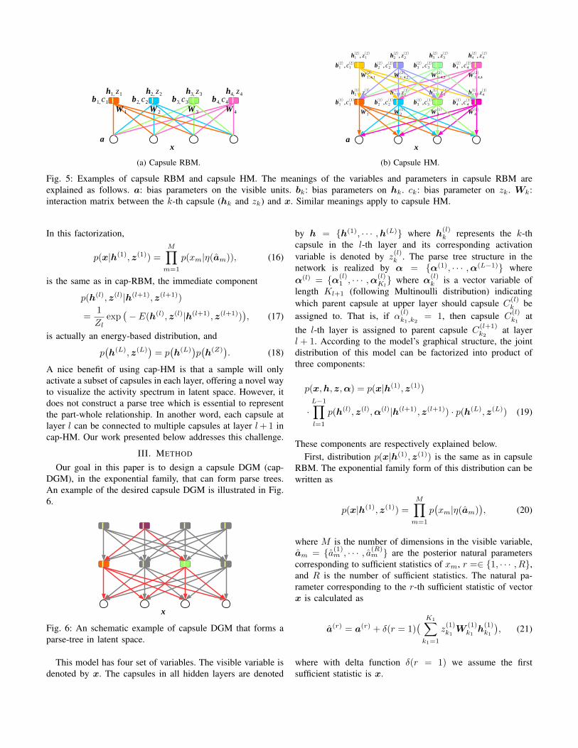
Fig. 5: Examples of capsule RBM and capsule HM. The meanings of the variables and parameters in capsule RBM areexplained as follows. a: bias parameters on the visible units. bk: bias parameters on hk. ck: bias parameter on zk. Wk:interaction matrix between the k-th capsule (hk and zk) and x. Similar meanings apply to capsule HM.
In this factorization,
p(x|h(1), z(1)) =
M∏m=1
p(xm|η(am)), (16)
is the same as in cap-RBM, the immediate component
p(h(l), z(l)|h(l+1), z(l+1))
=1
Zlexp
(− E(h(l), z(l)|h(l+1), z(l+1))
), (17)
is actually an energy-based distribution, and
p(h(L), z(L)
)= p(h(L)
)p(h(Z)
). (18)
A nice benefit of using cap-HM is that a sample will onlyactivate a subset of capsules in each layer, offering a novel wayto visualize the activity spectrum in latent space. However, itdoes not construct a parse tree which is essential to representthe part-whole relationship. In another word, each capsule atlayer l can be connected to multiple capsules at layer l+ 1 incap-HM. Our work presented below addresses this challenge.
III. METHOD
Our goal in this paper is to design a capsule DGM (cap-DGM), in the exponential family, that can form parse trees.An example of the desired capsule DGM is illustrated in Fig.6.
x
Fig. 6: An schematic example of capsule DGM that forms aparse-tree in latent space.
This model has four set of variables. The visible variable isdenoted by x. The capsules in all hidden layers are denoted
by h = {h(1), · · · ,h(L)} where h(l)k represents the k-th
capsule in the l-th layer and its corresponding activationvariable is denoted by z
(l)k . The parse tree structure in the
network is realized by α = {α(1), · · · ,α(L−1)} whereα(l) = {α(l)
1 , · · · ,α(l)Kl} where α(l)
k is a vector variable oflength Kl+1 (following Multinoulli distribution) indicatingwhich parent capsule at upper layer should capsule C
(l)k be
assigned to. That is, if α(l)k1,k2
= 1, then capsule C(l)k1
atthe l-th layer is assigned to parent capsule C
(l+1)k2
at layerl + 1. According to the model’s graphical structure, the jointdistribution of this model can be factorized into product ofthree components:
p(x,h, z,α) = p(x|h(1), z(1))
·L−1∏l=1
p(h(l), z(l),α(l)|h(l+1), z(l+1)) · p(h(L), z(L)) (19)
These components are respectively explained below.First, distribution p(x|h(1), z(1)) is the same as in capsule
RBM. The exponential family form of this distribution can bewritten as
p(x|h(1), z(1)) =
M∏m=1
p(xm|η(am)
), (20)
where M is the number of dimensions in the visible variable,am = {a(1)m , · · · , a(R)
m } are the posterior natural parameterscorresponding to sufficient statistics of xm, r =∈ {1, · · · , R},and R is the number of sufficient statistics. The natural pa-rameter corresponding to the r-th sufficient statistic of vectorx is calculated as
a(r) = a(r) + δ(r = 1)( K1∑k1=1
z(1)k1W
(1)k1h(1)k1
), (21)
where with delta function δ(r = 1) we assume the firstsufficient statistic is x.
Second, the conditional distribution in an intermediate layerp(h(l), z(l),α(l)|h(l+1), z(l+1)) is actually an energy-basedmodel:
p(h(l), z(l),α(l)|h(l+1), z(l+1)) =1
Zle−E(h(l),z(l),α(l)),
(22)
where Zl is the partition function, and in the language ofexponential family the energy function can be defined as
E(h(l), z(l),α(l)) = −Kl∑k1
J∑j=1
(b(l)k1,j
Tt(l)k1,j
+ log g(h(l)k1,j
))
− c(l)Tz(l) −
Kl∑k1=1
d(l)k1
Tα
(l)k1
−Kl∑
k1=1
Kl+1∑k2=1
α(l)k1,k2
z(l)k1z(l+1)k2
h(l)k1
TW
(l+1)k1,k2
h(l+1)k2
, (23)
where J is the length of a capsule h(l)k1
, t(l)k1is the corre-
sponding sufficient statistics, b(l)k1is the corresponding natural
parameter, c(l) is the natural parameter of Bernoulli vectorz(l), d(l)k1
is the natural parameter of Multinoulli distributionof vector α(l)
k1, and matrix W (l+1)
k1,k2is the transformation matrix
between capsule C(l)k1
and C(l+1)k2
.From this energy-based distribution, we can derive condi-
tionals of each individual variable, as below:
p(h(l)|z(l),α(l),h(l+1), z(l+1))
=
Kl∏k1=1
p(h(1)k1|z(l)k1
,α(l)k1,h(l+1), z(l+1))
=
Kl∏k1=1
p(h(l)k1|η(b
(l)k1
)), (24)
where
b(l,u)k1
= b(l,u)k1
+ δ(u = 1)
Kl+1∑k2=1
α(1)k1,k2
z(l)k1z(l+1)k2
W(l+1)k1,k2
h(l+1)k2
;
(25)
p(z(l)|h(l),α(l),h(l+1), z(l+1)
)=
Kl∏k1=1
p(z(l)k1|h(l)
k1,α
(l)k1,h(l+1), z(l+1)
)=
Kl∏k1=1
BE(z(l)k1|η(c
(l)k1
)), (26)
where z(l)k1
is a Bernoulli variable and its posterior naturalparameter is
c(l)k1
= c(l)k1
+
Kl+1∑k2=1
α(1)k1,k2
z(l+1)k2
h(l)k1
TW
(l+1)k1,k2
h(l+1)k2
; (27)
p(α(l)|h(l), z(l),h(l+1), z(l+1)
)=
Kl∏k1=1
p(α
(l)k1|h(l)
k1, z
(l)k1,h(l+1), z(l+1)
)=
Kl∏k1=1
MU(α
(l)k1|η(d
(l)k1
)), (28)
where α(l)k1
is a Multinoulli variable of length Kl+1 and itsposterior parameter is
d(l)k1
= d(l)k1
+
z(l)k1z(l+1)1 h
(l)k1
TW
(l+1)k1,1
h(l+1)1
z(l)k1z(l+1)2 h
(l)k1
TW
(l+1)k1,2
h(l+1)2
...
z(l)k1z(l+1)Kl+1
h(l)k1
TW
(l+1)k1,Kl+1
h(l+1)Kl+1
. (29)
For the top hidden layer, p(h(L), z(L)) can be simplyfactorized as
p(h(L), z(L)) = p(z)p(h|z), (30)
where p(z) follows a Multinoulli distribution, and p(h|z)follows a distribution from the exponential family.
Similarly, the joint distribution of the inference componentis written as
q(h, z,α|x) = q(h(1), z(1)|x)
·L−1∏l=1
q(h(l+1), z(l+1),α(l)|h(l), z(l)). (31)
First, q(h(1), z(1)|x) is the same as in capsule RBM.For 1 ≤ l ≤ L − 2, q(h(l+1), z(l+1),α(l)|h(l), z(l)) is an
energy-based submodel
q(h(l+1),z(l+1),α(l)|h(l),z(l)) =1
Z(R)l+1
e−E(h(l+1),z(l+1),α(l)),
(32)
where
E(h(l+1), z(l+1),α(l))
= −Kl+1∑k2=1
J∑j=1
(b(R,l+1)k2,j
Tt(l+1)k2,j
+ log g(h(l+1)k2,j
))
− c(R,l+1)Tz(l+1)
−Kl∑
k1=1
d(R,l)k1
Tα
(l)k1
−K1∑
k1=1
Kl+1∑k2=1
α(l)k1,k2
z(l)k1z(l+1)k2
h(l+1)k1
TW
(R,l+1)k1,k2
h(l+1)k2
.
(33)

The conditional distributions of this energy-based submodelcan be obtained as below:
q(h(l+1)|z(l+1),α(l),h(l), z(l))
=
Kl+1∏k2=1
q(h(l+1)k2|z(l+1)
k2,α(l),h(l), z(l))
=
Kl+1∏k2=1
q(h(l+1)k2|η(b
(R,l+1)k2
)), (34)
where
b(R,l+1,u)k2
= b(R,l+1,u)k2
+ δ(u = 1)
·Kl∑
k1=1
α(l)k1,k2
z(l)k1z(l+1)k2
h(l+1)k1
TW
(R,l+1)k1,k2
h(l+1)k2
; (35)
q(z(l+1)|h(l+1),α(l),h(l), z(l))
=
Kl+1∏k2=1
q(z(l+1)k2|h(l+1)
k2,α(l),h(l), z(l))
=
Kl+1∏k2=1
BE(z(l+1)k2|η(c
(R,l+1)k2
)), (36)
where
c(R,l+1)k2
= c(R,l+1)k2
+
Kl∑k1=1
α(l)k1,k2
z(l)k1h
(l+1)k1
TW
(R,l+1)k1,k2
h(l+1)k2
;
(37)
q(α(l)|h(l+1), z(l+1),h(l), z(l))
=
Kl∏k1=1
q(α(l)k1|h(l+1), z(l+1), z
(l)k1
)
=
Kl∏k1=1
MU(η(d
(R,l)k1
)), (38)
where
d(R,l)k1
= d(R,l)k1
+
z(l)k1z(l+1)1 h
(l)k1
TW
(R,l+1)k1,1
h(l+1)1
z(l)k1z(l+1)2 h
(l)k1
TW
(R,l+1)k1,2
h(l+1)2
...
z(l)k1z(l+1)Kl+1
h(l)k1
TW
(R,l+1)k1,Kl+1
h(l+1)Kl+1
. (39)
We assume z(L) is Multinoulli inq(h(L), z(L),α(L−1)|h(L−1), z(L−1)).
A. Model Learning
Obviously, the generative parameters include θ ={a, b, c,d,W }. The recognition parameters include φ ={b(R), c(R),d(R),W (R)}. Similar to the parameter learning incapsule HM, we can derive learning rules for capsule DGM:
∆θ =∂j(x)
∂θ= −Eq(h,z,α|x)
[∂ log p(x,h, z,α)
∂θ
]. (40)
Now, let us start with the gradient for W (l+1)kl,kl+1
below.
∂ log p(x,h,z,α)
∂W(l+1)kl,kl+1
=∂ log p
(h(l),z(l),α(l)|h(l+1),z(l+1)
)∂W
(l+1)kl,kl+1
=∂E(h(l),z(l),α(l))
∂W(l+1)kl,kl+1
− Ep(h(l),z(l),α(l)|h(l+1),z(l+1))
[∂E(h(l),z(l),α(l))
∂W(l+1)kl,kl+1
]=(α(l)kl,kl+1
z(l)klh
(l)kl− 〈α(l)
kl,kl+1z(l)klh
(l)kl〉)(z(l+1)kl+1
h(l+1)kl+1
)T, (41)
where 〈·〉 is the shorthand for expectation w.r.t. generativedistribution p(x,h, z,α), and variables outside 〈·〉 are sam-pled from the recognition distribution q(h, z,α|x) (actuallythey are mean-field approximations).
Similarly, the gradients for b, c, and d can be computed asbelow
∂ log p(x,h, z,α)
∂b(l,u)k
= t(l,u)k − 〈t(l,u)k 〉, (42)
∂ log p(x,h, z,α)
∂c(l)= z(l) − 〈z(l)〉, (43)
∂ log p(x,h, z,α)
∂d(l)kl,kl+1
= α(l)kl,kl+1
− 〈α(l)kl,kl+1
〉. (44)
Using the same spirit, we can compute gradients for recog-nition parameters using the master equation below.
∆φ =∂j(x)
∂φ= −Ep(x,h,z,α)
[∂ log q(h, z,α|x)
∂φ
]. (45)
∂q(h,z,α|x
)∂W
(R,l+1)kl,kl+1
=∂q(h(l+1),z(l+1),α(l)|h(l),z(l)
)∂W
(R,l+1)kl,kl+1
=∂E(h(l+1),z(l+1),α(l))
∂W(R,l+1)kl,kl+1
− Eq(h(l+1),z(l+1),α(l)|h(l),z(l))
[∂E(h(l+1),z(l+1),α(l))
∂W(R,l+1)kl,kl+1
](46)
=(z(l)klh
(l)kl
)(α(l)kl,kl+1
z(l+1)kl+1
h(l+1)kl+1
− 〈α(l)kl,kl+1
z(l+1)kl+1
h(l+1)kl+1〉)T.
(47)
Similarly, we can have
∂ log q(h, z,α|x)
∂b(R,l,u)k
= t(l,u)k − 〈t(l,u)k 〉, (48)
∂ log q(h, z,α|x)
∂c(R,l)= z(l) − 〈z(l)〉, (49)
∂ log q(h, z,α|x)
∂d(R,l)kl,kl+1
= α(l)kl,kl+1
− 〈α(l)kl,kl+1
〉, (50)
where 〈·〉 is the expectation under recognition distributionq(h, z,α|x), and variables outside are sampled (mean-fieldapproximated) from the generative distribution p(x,h, z,α).

(a) Pretrain first capsule RBM. (b) Pretrain first capsule RBM. (c) Fine-tuning.
Fig. 7: Learning curves of cap-DGM in terms of reconstruction error in pretraining and finetuning phases on MNIST.
IV. PRELIMINARY EXPERIMENTS
We conducted a set of preliminary experiments on theMNIST and Fashion-MNIST data. First of all, we learneda cap-DGM, on both datasets, with two latent layers ofcapsules, each of which has 40 capsules and each capsulehas 9 Gaussian variables. The network was layer-wise pre-trained as cap-RBMs, and then finetuned using our wake-sleep learning algorithm. The pretraining phase is essentialto help initialize the model parameters. The learning curvesin terms of reconstruction error in both phases on MNIST areshown in Fig. 7. It shows that both training phases graduallyreduce the reconstruction error. The learning of cap-RBMsdoes help guide the learning of the entire network into acomfort parameter space. In our experiments, we found thatthe learning of cap-DGM would not be successful withoutpretraining.
After model learning, we generated parse trees for realsamples from the data and visualized it in Fig. 8 and 9. Itcan be seen that in each case, a tree structure indeed wasconstructed with the parent capsules on the top layer andchild capsules at the bottom layer. Each child capsule is onlyconnected to just one parent capsule, which is an advantageover the activity spectra of capsules from cap-HM reportedin [11]. Further more, from these parse trees, we can observethat different samples from the same class obtain similar butnot identical structures, and parse trees across different classesexhibit distinct patterns. Thus, it contributes a novel way ofvisualizing the latent space in deep generative models.
Due to the property that the structure of a tree expandsexponentially as the increase of depth, the parse tree cannot be very deep. But by adding one more latent capsulelayers, we can observe, e.g. from Fig. 10, parse trees moreclearly for corresponding samples. Again, in contrast to theresults reported in [11], it implies that our new model helpsenforce more structured latent space than cap-HM (providingspectrum-like structure) and other deep generative models suchas VAE [17] (providing full connections between layers).
V. DISCUSSION AND CONCLUSION
It is a challenging task to model hierarchically structuredlatent space in deep generative models. In this paper, wepresent a novel capsule deep generative model, from theperspective of exponential family, that can form parse trees
(a) Actual MNIST samples. (b) Reconstructed samples.
(c) Parse trees for first 3 samples of digit 0 in (a) and (b).
(d) Parse trees for first 3 samples of digit 6 in (a) and (b).
(e) Parse trees ffor first 3 samples of digit 7 in (a) and (b).
Fig. 8: Reconstructed MNIST samples and correspondingparse trees from a cap-DGM with two latent capsule layers.Visible layer is not visualized in the trees. Size of a nodeindicates the activity of the capsule.

(a) Actual Fashion-MNIST samples. (b) Reconstructed samples.
(c) Parse trees for first three trousers in (a) and (b).
(d) Parse tree for first three sneakers in (a) and (b).
(e) Parse tree for first three ankle boots in (a) and (b).
Fig. 9: Reconstructed Fashion-MNIST samples and corre-sponding parse trees from a cap-DGM with two latent capsulelayers. Visible layer is not visualized in the trees. Size of anode indicates the activity of the capsule.
in the latent space to represent part-whole relationship. Ourpreliminary experimental results show that such tree structurescan be automatically learned from the data using our model.Please be reminded that, this work is a position paper, provingthe concept, but needing more studies and improvementsin implementation, learning algorithms, and validations. Wederived the wake-sleep learning algorithm for our model. Toimprove learning quality and possibly eliminate the pretrainingphase, new learning algorithms (such as REINFORCE method[16] and back-propagation [17], [18]) will be explored. Themethod is currently implemented using pure Python. It willbe re-designed in PyTorch or TensorFlow so that componentssuch as convolution can be added to the structure for better
Fig. 10: Parse trees of corresponding Fashion-MNIST samplesfrom a cap-DGM of three latent layers.
quality of generation.
ACKNOWLEDGMENT
The authors would like to thank the anomynous reviewersand all organisers of the conference.
REFERENCES
[1] G. Hinton, S. Osindero, and Y. Teh, “A fast learning algorithm for deepbelief nets,” Neural Computation, vol. 18, pp. 1527–1554, 2006.
[2] G. Hinton and R. Salakhutdinov, “Reducing the dimensionality of datawith neural networks,” Science, vol. 313, pp. 504–507, 2006.
[3] Y. LeCun, Y. Bengio, and G. Hinton, “Deep learning,” Nature, vol. 521,pp. 436–444, 2015.
[4] G. Hinton, J. McClelland, and D. Rumelhart, “Distributed repre-sentations,” in Parallel Distributed Processing: Explorations in TheMicrostructure of Cognition, D. Rumelhart and J. McClelland, Eds.Cambridge, MA: MIT Press, 1986, pp. 77–109.
[5] Y. Bengio, R. Ducharme, P. Vincent, and C. Jauvin, “A neural proba-bilistic language model,” Journal of Machine Learning Research, vol. 2,pp. 1137–1155, 2003.
[6] T. Mikolov, K. Chen, G. S. Corrado, and J. Dean, “Efficient estimationof word representations in vector space,” in International Conference onLearning Representations, 2013.
[7] Y. LeCun and Y. Bengio, “Convolutional networks for images, speech,and time series,” in The Handbook of Brain Theory and Neural Net-works, M. Arbib, Ed. Cambridge, MA: MIT Press, 1995, pp. 255–258.
[8] A. Krizhevsky, I. Sutskever, and G. E. Hinton, “ImageNet classificationwith deep convolutional neural networks,” in Advances in Neural Infor-mation Processing Systems 25, F. Pereira, C. J. C. Burges, L. Bottou, andK. Q. Weinberger, Eds. Curran Associates, Inc., 2012, pp. 1097–1105.
[9] S. Sabour, N. Frosst, and G. Hinton, “Dynamic routing between cap-sules,” in Neural Information Processing Systems, 2017, pp. 3856–3866.
[10] G. Hinton, S. Sabour, and N. Frosst, “Matrix capsules with EM routing,”in International Conference on Learning Representations, 2018.
[11] Y. Li and X. Zhu, “Capsule generative models,” in International Confer-ence on Artificial Neural Networks, Munich, Germany, Sep. 2019, pp.281–295.
[12] G. Hinton, A. Krizhevsky, and S. Wang, “Transforming auto-encoder,”in International Conference on Artificial Neural Networks, 2011, pp.44–51.
[13] M. Welling, M. Rosen-Zvi, and G. Hinton, “Exponential family har-moniums with an application to information retrieval,” in Advances inNeural Information Processing Systems, 2005, pp. 1481–1488.
[14] Y. Li and X. Zhu, “Exponential family restricted Boltzmann machinesand annealed importance sampling,” in International Joint Conferenceon Neural Networks, 2018, pp. 39–48.
[15] ——, “Exploring Helmholtz machine and deep belief net in the ex-ponential family perspective,” in ICML 2018 Workshop on TheoreticalFoundations and Applications of Deep Generative Models, 2018.
[16] R. J. Williams, “Simple statistical gradient-following algorithms forconnectionist reinforcement learning,” Machine Learning, vol. 8, pp.229–256, 1992.
[17] D. Kingma and M. Welling, “Auto-encoding variational Bayes,” inInternational Conference on Learning Representations, 2014.
[18] D. J. Rezende, S. Mohamed, and D. Wierstra, “Stochastic backprop-agation and approximate inference in deep generative models,” inInternational Conference on Machine Learning, 2014, pp. II–1278–II–1286.