Capter 16Output and Aggregate Demand

1

Chapter 16: Begg, Vernasca, Fischer, Dornbusch (2012).McGraw Hill

Learning ObjectivesPotential output vs. current outputDistinguish between autonomous expenditure

and induced expenditure and explain how real GDP influences expenditure plans

Explain how real GDP adjusts to achieve equilibrium expenditure

Explain the expenditure multiplier

2

Aggregate Output

Full employment output (or potential output) is the level of output produced when the labor market is in equlibrium and the economy is producing at full employment

Potential output is not the maximum level of output an economy can produce

3

Aggregate Output

Potential output reflects the level of labour that workers wish to supply

Current output what is currently produced, and might be diverge from potential output

4

The Aggregate Expenditure Model

Prices and wages are fixedOutput is determined by the demand sideFor the time being, we assume that there is

noGovernmentForeign Trade

5

The Aggregate Expenditure ModelA model that explains what determines the

quantity of real GDP demanded and changes in that quantity at a given price level

Aggregate Expenditure: Consumption, and Investment

6

The Aggregate Expenditure Model

The key assumption is that we divide expenditure plans into:

Autonomous expenditure does not respond to changes in real GDP

Induced expenditure does respond to changes in real GDP

7

The Consumption Function

All income is either spent on consumption or saved in an economy in which there are no taxes

Saving = Aggregate Income-Consumption

8

The Consumption Function

Some of the determinants of aggregate consumption:Household IncomeHousehold WealthInterest ratesHousehold’s expectations about the future

9

The Consumption Function

In the General theory, Keynes argued that consumption depends directly on income

Consumption function:

C =A+ cY

10

The Consumption Function

The slope of the consumption function (c) is called the marginal propensity to consume (MPC), or the fraction of a change in income that is consumed, or spent, 0<c<1

11

The Consumption Function

12

C = b + cY

∆C

∆Y c

∆Y

∆C

A

The Consumption FunctionThe fraction of a change in income that is

saved is called the marginal propensity to save (MPS).

Once we know how much consumption will result from a given level of income, we know how much saving there will be. Therefore,

13

1MPC + MPS

S Y C

The Consumption Function

C Y 1 0 0 7 5.

14

At a national income of zero, consumption is $100 billion (a).

For every $100 billion increase in income (Y), consumption rises by $75 billion (C).

The Consumption Function

15

)( TY =Disposable Income (DI) (Income - Net Taxes)

C = A + c (Y – T) A = autonomous consumption expenditure

c = marginal propensity to consume

The Determinants of Consumption

Expectations: a more optimistic outlook on the economy will raise consumer’s expenditures

The interest rate cause consumers to postpone consumption

Others: price level, and wealth

16

Changes in the Consumption Function

Consumption expenditure increases and the consumption function shifts upward if

• The real interest rate falls

• Wealth increases

• Expected future income increases

17

Real interest rates falls, wealth increases, expected future income increases

Changes in Consumption Function

18

ysyshsjjahbjjhdbfkjslkjbaslkjnaslkjcnbaklsjcnalijksxncsjsbjbjhbjbjhbjbjhbjbjhabjhsbjhbashb

ysyshsjjahbjjhdbfkjslkjbaslkjnaslkjcnbaklsjcnalijksxncsjsbjbjhbjbjhbjbjhbjbjhabjhsbjhbashb

ysbjhbashb

Real interest rates increases, wealth decreases, expected future income decreases

The Saving Function

19

C Y 1 0 0 7 5.S Y C

Y - C = S

AGGREGATEINCOME

(Billions of Dollars)

AGGREGATE CONSUMPTION

(Billions of Dollars)

AGGREGATE SAVING

(Billions of Dollars)

0 100 -100

80 160 -80

100 175 -75

200 250 -50

400 400 0

600 550 50

800 700 100

1,000 850 150

Investment

Investment refers to purchases by firms of new buildings and equipment and additions to inventories, all of which add to firms’ capital stock.

One component of the inventory is determined by how much households decide to buy, which is not under complete control of firms

20

Investment

Change in Inventory = Production - Sales

21

Actual versus Planned Investment

Desired or Planned investment refers to the additions to capital stock and inventory that are planned by firms.

Actual Investment is the actual amount of investment that takes place; it includes items such as unplanned changes in inventories

22

The Planned Investment Function

For now, we assume that planned investment is fixed

That is, it does not change when income changes

The planned investment is an autonomous variable

23

The Planned Investment Function

24

Investment Function

Investment is autonomous (independent of income)

25

II

Investment FunctionAt this point investment is planned

investment expenditures (I)Investment is closely linked to the

interest rate, since interest represents the opportunity cost of investing in capital

The investment function will shift with changes in expectations for business profits

26

Autonomous Investment

Although investment is related to the interest rate and business expectations, investment does not depend in any significant way on disposable income As such, investment is “autonomous”

However, changes in the interest rate or expectations for profits will still shift autonomous investment

27

Determinants of InvestmentFactors that can cause a shift in the investment function are:The interest rateExpectationsTechnology

28

Planned Aggregate Expenditure = Aggregate Demand

Planned aggregate expenditure is the total amount the economy plans to spend in a given period. It is equal to Aggregate Demand. It is equal to consumption (C) plus planned investment (I).

29

IC AD

Aggregate Demand

30

Equilibrium

In the macroeconomics good market, equilibrium occurs when desired spending equals to aggregate output, income

31

EquilibriumOutput = Desired Spending

Y =AD = C + IDisequilibria

Output > Desired SpendingOutput < Desired Spending

32

Equilibrium

33

C Y 1 0 0 7 5. I 2 5Deriving the Desired Spending Schedule and Finding Equilibrium (All Figures in Billions of Dollars) The Figures in Column 2 are Based on the Equation C = 100 + .75Y.

(1) (2) (3) (4) (5) (6)

AGGREGATEOUTPUT

(INCOME) (Y)

AGGREGATECONSUMPTION (C)

PLANNEDINVESTMENT (I)

DESIRED (AD)C + I

UNPLANNEDINVENTORY

CHANGEY (C + I)

EQUILIBRIUM?(Y = AD)

100 175 25 200 100 No

200 250 25 275 75 No

400 400 25 425 25 No

500 475 25 500 0 Yes

600 550 25 575 + 25 No

800 700 25 725 + 75 No

1,000 850 25 875 + 125 No

Y Y 1 0 0 7 5 2 5.

Y C I (1)

C Y 1 0 0 7 5.(2)

I 2 5(3)

By substituting (2) and (3) into (1) we get:

There is only one value of Y for which this statement is true. We can find it by rearranging terms:

Y Y 1 0 0 7 5 2 5.

Y Y .7 5 1 0 0 2 5Y Y .7 5 1 2 5

.2 5 1 2 5Y

Y 1 2 5

2 55 0 0

.

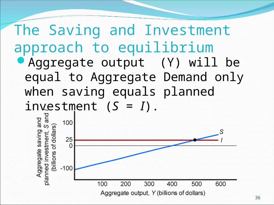
The Saving and Investment approach to equilibriumAggregate output (Y) will be equal

to Aggregate Demand only when saving equals planned investment (S = I).

36

The MultiplierThe multiplier is the ratio of the change

in the equilibrium level of output to a change in some autonomous variable.An autonomous variable is a variable that is assumed not to depend on the state of the economy—that is, it does not change when the economy changes.

In this chapter, for example, we consider planned investment to be autonomous

37

The MultiplierThe multiplier of autonomous

investment describes the impact of an initial increase in planned investment on production, income, consumption spending, and equilibrium income.

The size of the multiplier depends on the slope of the planned aggregate expenditure line.

38

The MultiplierThe marginal propensity to save may

be expressed as:

Because S must be equal to I for equilibrium to be restored, we can substitute I for S and solve:

39

M P SS

Y

M P SI

Y

Y IM P S

1

m ultip lierM P C

1

1

The Multiplier

40

After an increase in planned investment, equilibrium output is four times the amount of the increase in planned investment.

The Paradox of Thrift

When households become concerned about the future and decide to save more, the corresponding decrease in consumption leads to a drop in spending and income.

Households end up consuming less, but they have not saved any more.