CARICOOS:UnSistemaCaribeñoparalaObservaciónCostera

JulioM.MorellRodriguez

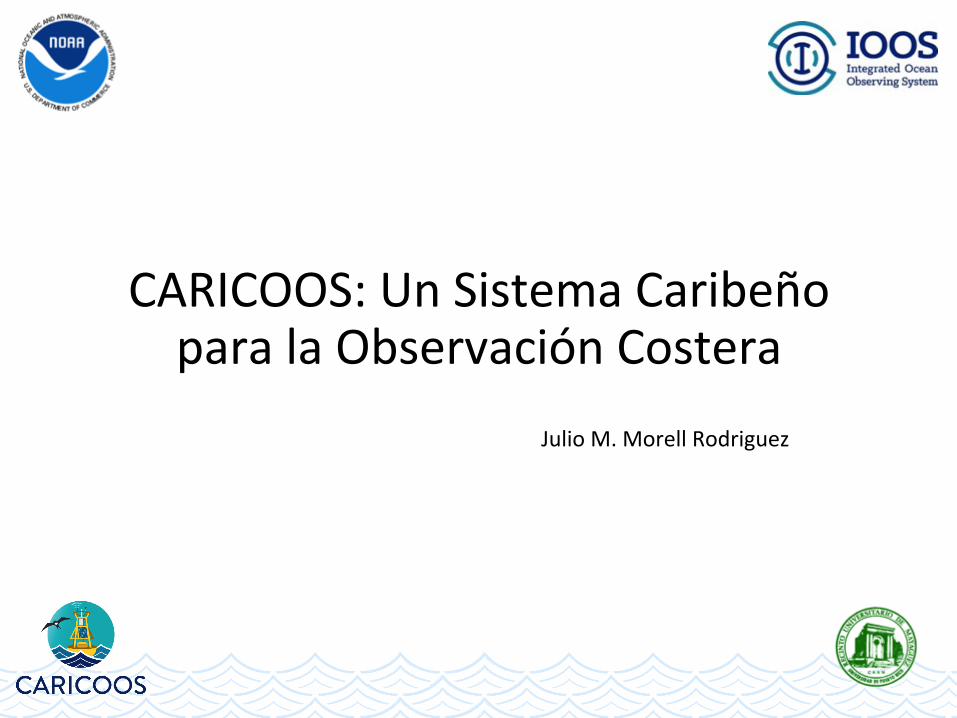
LaregiónCariCOOS:•  Elevaciónmax.1.2km•  Zpromediooceánica:4km•  Zpromedioplataforma:25m•  Pendientesmarcadas

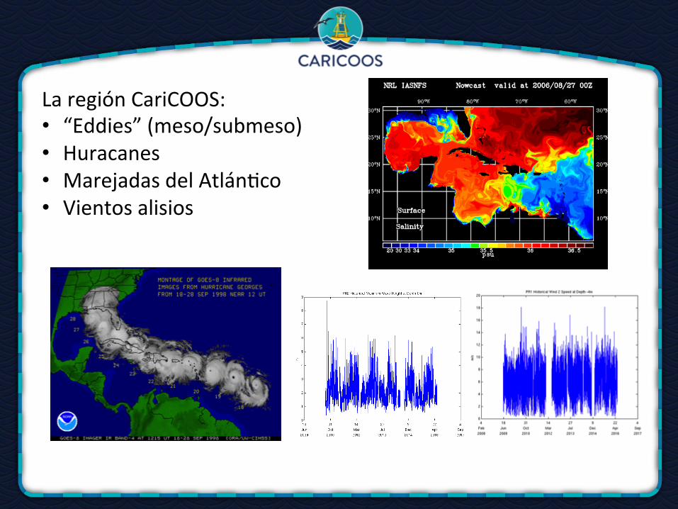
LaregiónCariCOOS:•  “Eddies”(meso/submeso)•  Huracanes•  MarejadasdelAtlánTco•  Vientosalisios

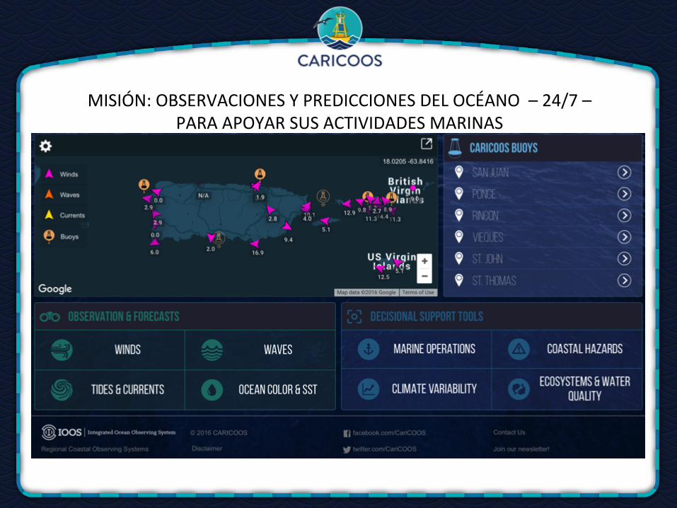
MISIÓN:OBSERVACIONESYPREDICCIONESDELOCÉANO–24/7–PARAAPOYARSUSACTIVIDADESMARINAS

MAUNABO HFR Antenna

LAS MAREAS Meteo Station

PONCE Data Buoy

SEAGLIDER 1 (variable location)

PONCE HFR

Antenna ISLA

MAGUEYES Meteo Station

LA PARGUERA

MapCO2 Buoy

SOUTH CABO ROJO HFR Antenna

SOUTH CABO ROJO Meteo Station

NORTH CABO ROJO HFR Antenna

NORTH CABO ROJO Meteo Station

AÑASCO HFR Antenna

RINCON Wave Buoy

RINCON Meteo Station

AGUADILLA Meteo Station

ARECIBO Meteo Station SAN JUAN

Meteo Station

SEAGLIDER 2 (variable location)

SAN JUAN Data Buoy

GURABO Meteo Station

TWO BROTHERS Meteo Station CROWN MOUNTAIN

Meteo Station SAVANAH ISLAND

Meteo Station

FAJARDO Meteo Station

VIEQUES Data Buoy ST JOHN

Data Buoy

SANDY POINT Meteo Station

BUCK ISLAND Meteo Station

RUPERTS ROCK Meteo Station

ST THOMAS

Data Buoy

YABUCOA Meteo Station

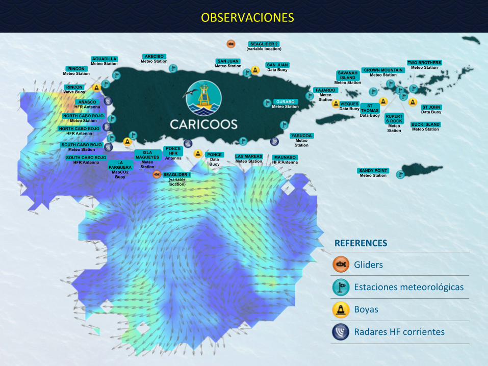
Gliders

Estacionesmeteorológicas

Boyas

RadaresHFcorrientes

REFERENCES

OBSERVACIONES

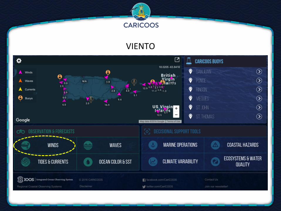
VIENTO

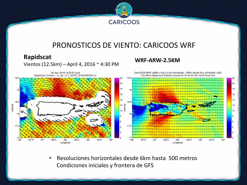
PRONOSTICOSDEVIENTO:CARICOOSWRFRapidscatVientos(12.5km)–April4,2016~4:30PM

WRF-ARW-2.5KM

•  Resolucioneshorizontalesdesde6kmhasta500metrosCondicionesinicialesyfronteradeGFS

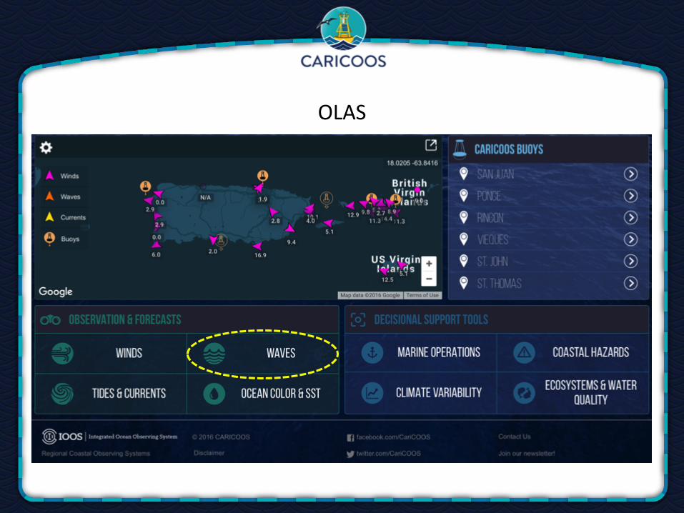
OLAS

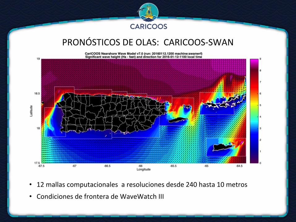
PRONÓSTICOSDEOLAS:CARICOOS-SWAN

•  12mallascomputacionalesaresolucionesdesde240hasta10metros

•  CondicionesdefronteradeWaveWatchIII

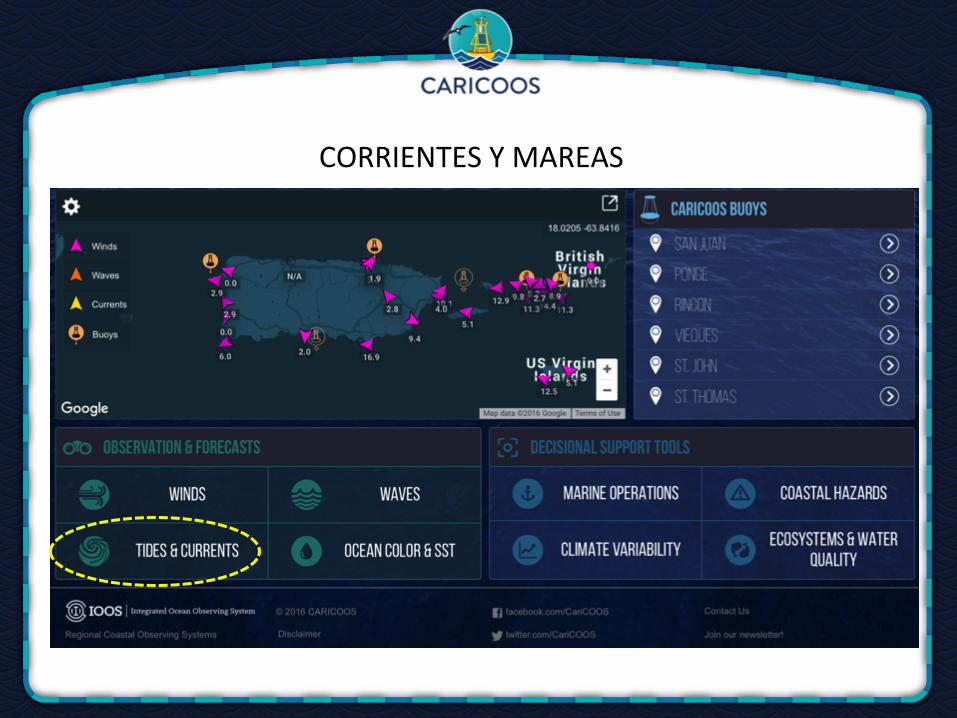
CORRIENTESYMAREAS

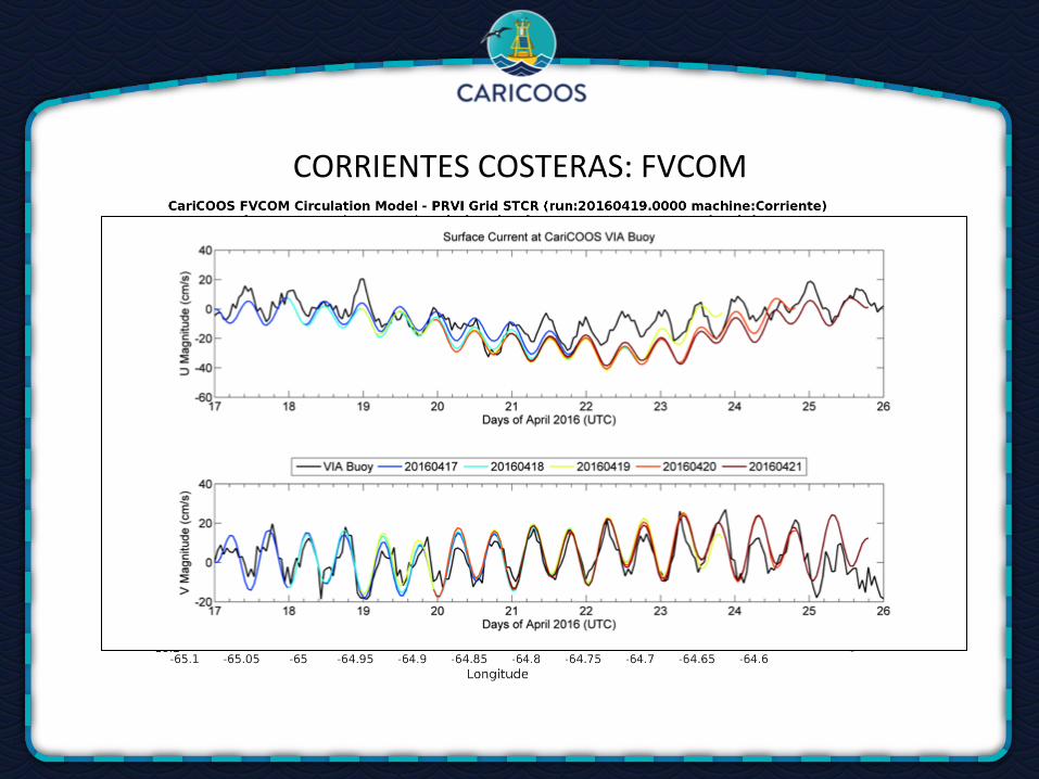
CORRIENTESCOSTERAS:FVCOM

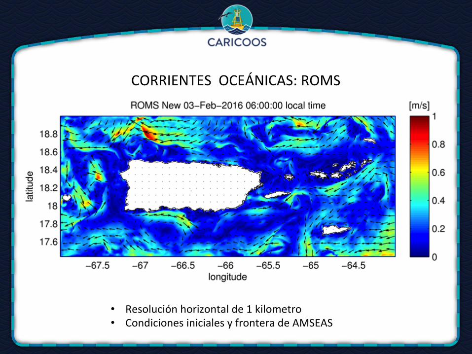
CORRIENTESOCEÁNICAS:ROMS

•  Resoluciónhorizontalde1kilometro•  CondicionesinicialesyfronteradeAMSEAS

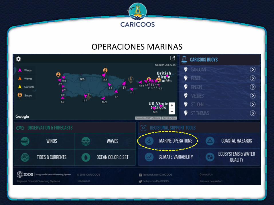
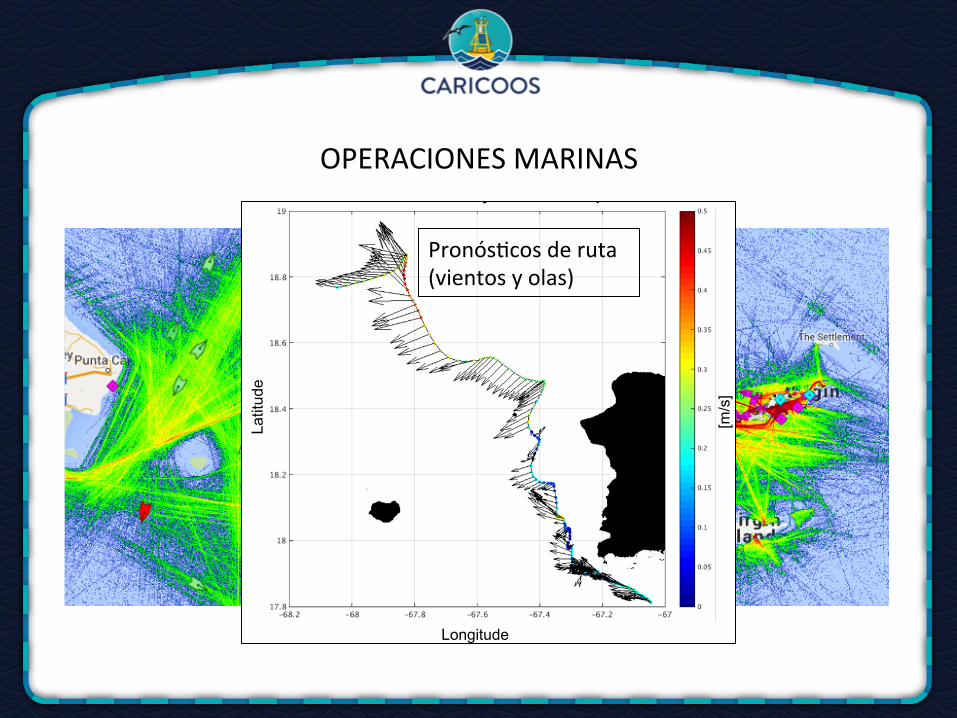
OPERACIONESMARINAS

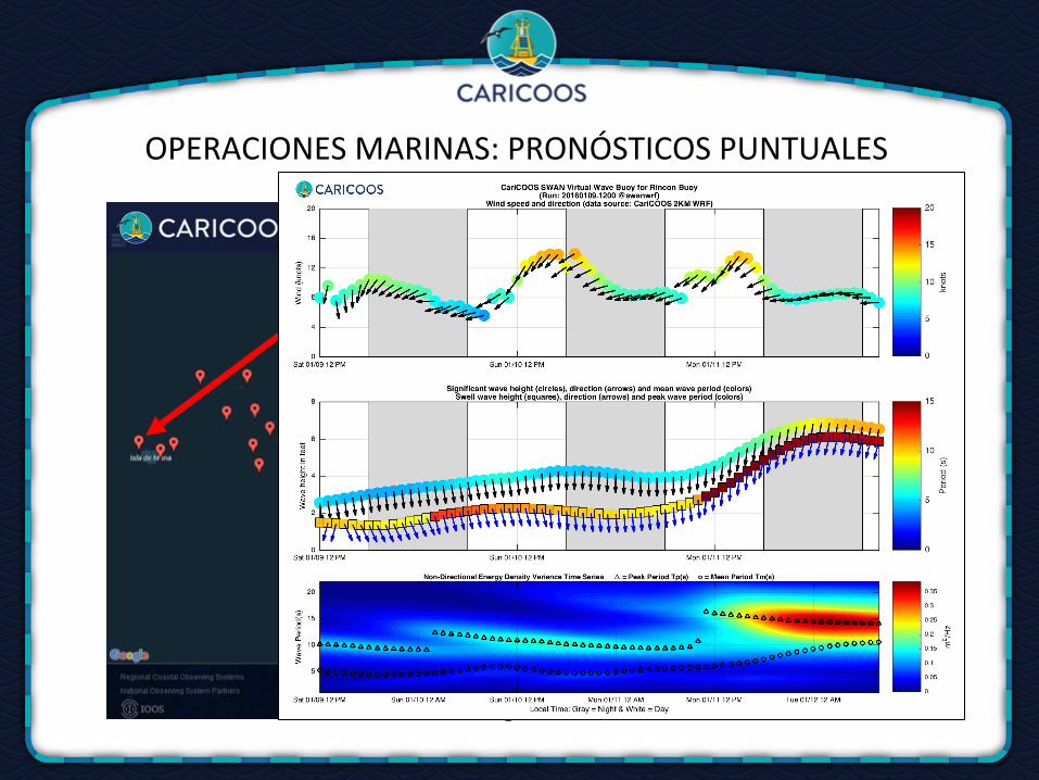
OPERACIONESMARINAS:PRONÓSTICOSPUNTUALES

•  Over200CariCOOSpointforecast•  Majorusers:recrea=onalboaters,commercialfishing,lawenforcement,surfers&beachgoers

The Mona Passage is dominated by very complex circulation patterns caused by the interaction between strong tidal currents,large-scale circulation and mesoscale phenomena. Seven-teen satellite-tracked drifters were deployed on or near the MonaPassage between February 2015 and August 2015. These deployments aimed to determine the transport of fish eggs andearly larvae from several marine protected areas (MPAs) off the west coast of Puerto Rico. These drifters transmitted theirlocation every half hour; individually providing continuous data for a maximum of two months, but, as a whole, providingcontinuous data for almost five months. The data acquired from these deployments has allowed for the direct observation ofthe main features of the circulation in the Mona Passage.

Langrangian Drifter Dispersion in the Mona PassageEstefanía Quiñones-Meléndez1, Miguel Canals2, and Jorge E. Capella3

estefania.quinones@upr.edu1Physical Oceanography, Department of Marine Sciences, University of Puerto Rico at Mayagüez

2UPRM Center for Applied Ocean Sciences and Engineering, Dept. of Engineering Science and Materials, University of Puerto Rico at Mayagüez3Caribbean Coastal Ocean Observing System, University of Puerto Rico at Mayagüez

Poulain, P. (2001). Adriatic Sea surface circulation as derived from drifter data between 1990 and 1999. Journal of MarineSystems, 29 (1-4), 3-32. This project is funded by the NOAA Coral Reef Conservation Program, Grant FNA14NMF4410150.

Drifter 3 DesecheoDrifter 4 BdSDrifter 5 BdSDrifter 6 BdSDrifter 7 BdS

The first group of drifters released on Feb. 5, 2015 and Feb. 11, 2015 are shown. Theinserted table lists the deployment site and colored path that corresponds to each drifter.

Drifter 3 transmitted its position every 30 min. until March 8, 2015 at 10:48PM(EST). Due to battery loss, its last recorded position is about 115 kilometers offthe north coast of Haiti.

Trajectories for drifters 3 through 19

Latit

ude

Longitude

Day

s A

fter D

eplo

ymen

t

Latit

ude

Longitude

Day

s A

fter R

elea

se

Traj

ecto

ries

upda

ted

on F

ebru

ary

26, 2

015

Latit

ude

Day

s A

fter R

elea

se

Trajectories for drifters 3 through 19 [zoom-in]

Latit

ude

Longitude

[m/s

]

3 % of WRF wind velocity at drifter 17’s positions

Dis

tanc

e [k

m]

Time [# of days]

Drifters’ Trajectories

Speeds for drifters 3 through 19

[kts

]

Visual comparison of drifter trajectories and their corresponding speeds. These images help show the drifters coveragearea and identify the location of stronger and weaker currents.

Simulated Larval Dispersal

Drifter 3 DesecheoDrifter 4 BdSDrifter 5 BdSDrifter 6 BdSDrifter 7 BdS

Longitude

Wind Slip

The C.O.D.E drifters were designed to reduce wind drag,but the effect is still present. Recent works revealed thatthe wind slip is 3% of the present wind forcing. Wecalculated the 3% of the WRF wind model for our regionand plotted it on top of the drifter trajectories for a bettervisualization.

Data Distribution

[Above] The Mona Passage area was divided in 0.1° x 0.1° bins.Colorbar represents the density of valid data points per bin.[Right] Trajectories of 336 virtual particles followed during twoweeks based on the AMSEAS hydrodynamic model. Particleswere released one-by-one every 3 hours starting on December1st, 2014 up to May 17, 2015.

Two-Particle Statistics / Relative Dispersion

Visual representation of how far away drifters travelled fromtheir initial position with respect to the number of days atsea. The behavior is very similar between drifters andindependent of the deployment site.

Single Particle Statistics / Absolute DispersionIntroduction

Dis

tanc

e [k

m]

Distance between drifter 3 and concurrent drifters

Distance travelled from deployment site

Source refers to Bajo de Sico(18.2300, -67.4299). All 17 drifters were referenced to this starting point.

Radial distance from source in 1(black) and 2(red) weeks

Mona Passage Circulation

This close-up shows the drifters’ sensitivity to tidalfluctuations, and a glimpse of the dominant northwarddirections of the currents in the Mona Passage. Cautionmust be take before identifying eddies, this image coversa span of 14 days worth of data, it is not a snapshot ofconditions at an specific instant of time.La

titud

e

Longitude

Next StepsWe are currently developingthe design for an eco-friendlyversion of the C.O.D.E drifter.The preliminary plans includeusing bamboo trunks as asubstitute for the PVC tubesand cotton fabric for the vanes.

References and AcknowledgementsDate

Drifter position data was interpolated to an hourly time step. Distance between pairs of drifters were calculated for those that were active at the same time. This image shows the case for drifter 3, which shared active time with drifters 4, 5, 6, and 7.

PronósTcosderuta(vientosyolas)

OPERACIONESMARINAS

Clickonvirtualbuoy

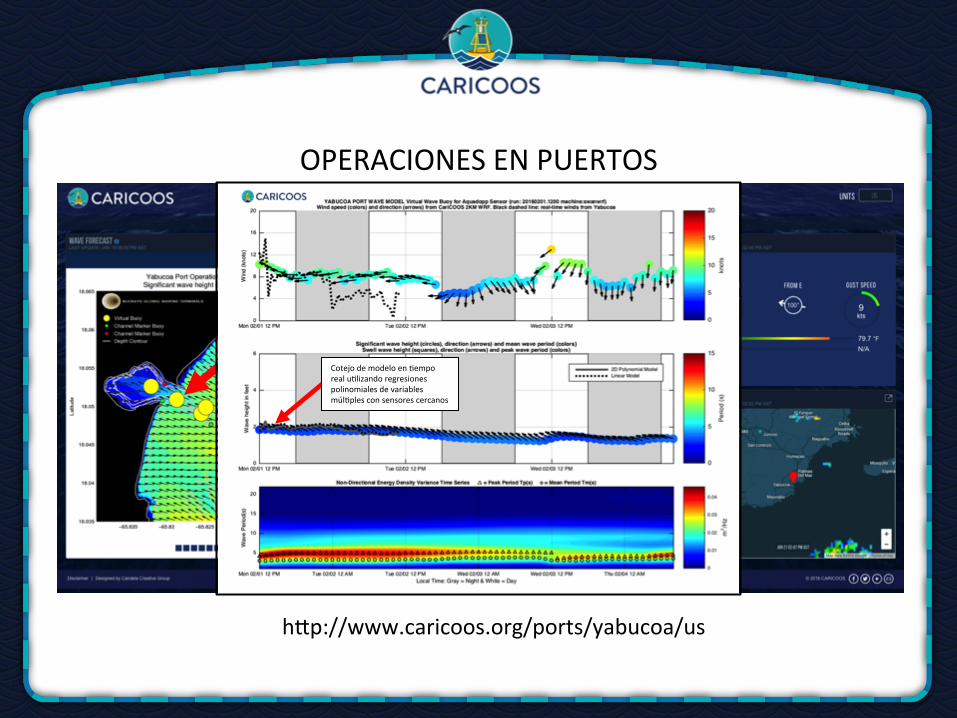
CotejodemodeloenTemporealuTlizandoregresionespolinomialesdevariablesmúlTplesconsensorescercanos

hlp://www.caricoos.org/ports/yabucoa/us

OPERACIONESENPUERTOS

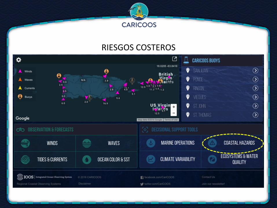
RIESGOSCOSTEROS

Beach Hazards Warning System Final Report

where d is the local water depth and L is the local wavelength, which is obtained by solving the fullwave dispersion relation:

!2 = gk tanh kd (3.5)

where ! = 2⇡/T is the wave angular frequency and k = 2⇡/L is the angular wavenumber.

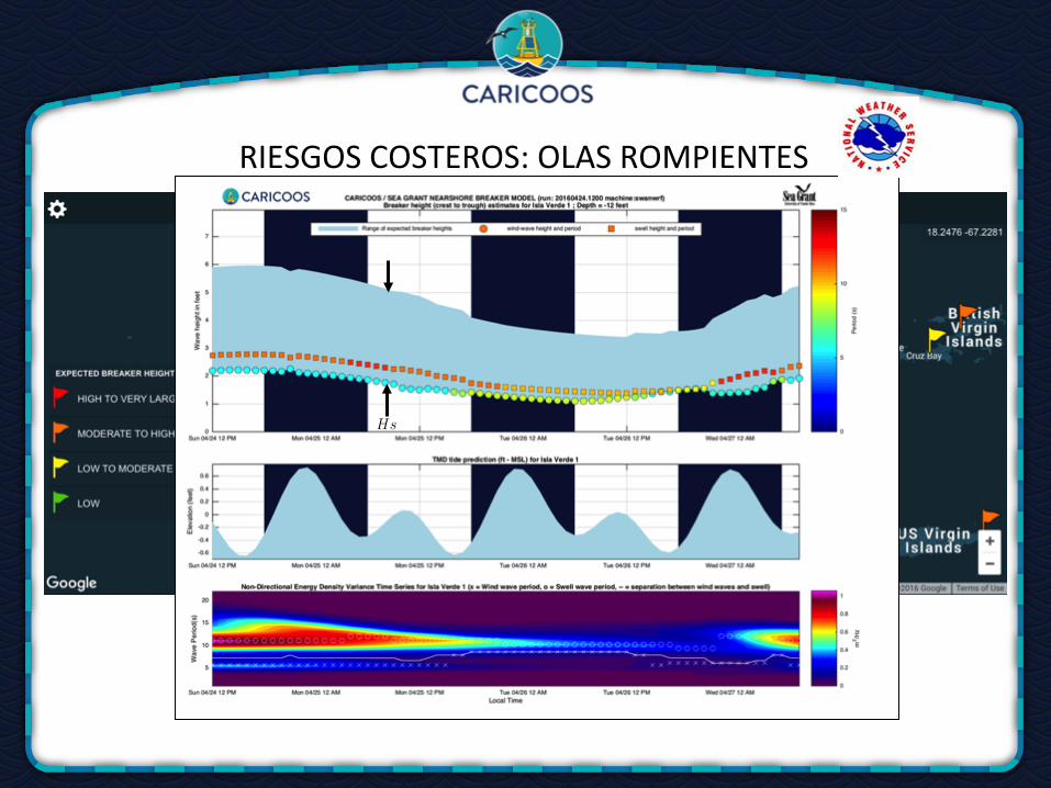
In order to estimate breaking wave heights, a similar approach was used in the present study in whichthe time-dependent wave energy flux at each virtual buoy is computed using equation 3.2 and then usedto calculate the equivalent offshore wave height so that equation 3.1 by (?) can be used to estimate thetime-dependent breaking wave heights. The SWAN model output at each virtual buoy is characterizedby the predicted significant wave height Hsi, mean wave period Tmi, peak wave period Tpi, the swellwave height Hswi, the mean wave direction ✓mi, and peak wave direction ✓pi. The i subscript indicatesthat this is the model estimated wave parameter at a specific nearshore virtual buoy. The time-dependentwave-energy flux at each virtual buoy is then calculated as:

Pi(t) = Ei(t)Cgi(t) (3.6)

where

Ei(t) =1

8⇢gHs2i (3.7)

and

Cgi(t) =1

2

(

1 +4⇡di/Li

sinh(4⇡di/Li)

)Li

Tpi(3.8)

where Cgi is the group speed at the virtual buoy location, di is the water depth at the virtual buoy andLi is the wavelength corresponding to the SWAN-predicted peak wave period Tpi, computed using thefull dispersion relation given in equation 3.5. Using equation 3.2, the equivalent deep water wave heightH1 with an energy flux equal to the energy flux predicted by SWAN at the virtual buoy location is givenby

H1 = Hsi

sCgiCg1

(3.9)

where Cg1 is the deep water group speed corresponding to the SWAN-predicted peak wave periodat the virtual buoy location, Tpi. Using this equivalent deep water wave height, it is then possible toestimate the breaking wave height based on the available wave energy flux at the virtual buoy location,using ?’s relationship:

Preliminary draft 24

RIESGOSCOSTEROS:OLASROMPIENTES

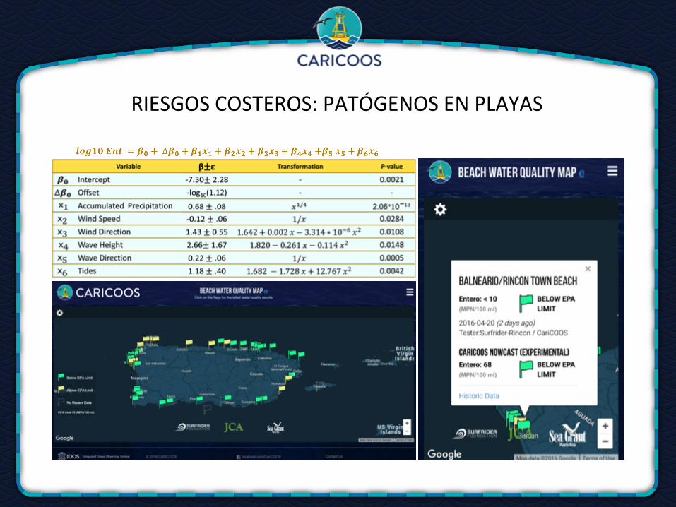
RIESGOSCOSTEROS:PATÓGENOSENPLAYAS

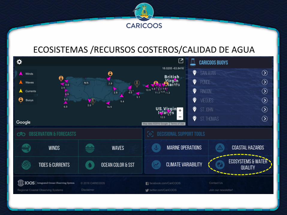
ECOSISTEMAS/RECURSOSCOSTEROS/CALIDADDEAGUA

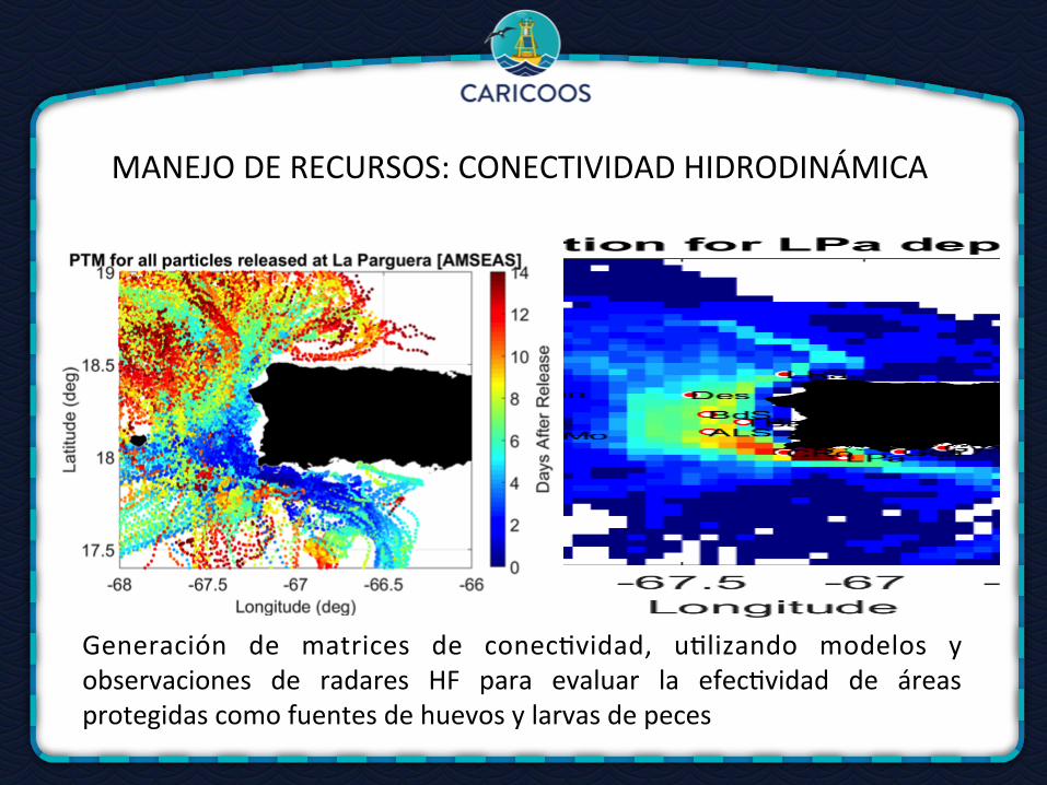
Generación de matrices de conecTvidad, uTlizando modelos yobservaciones de radares HF para evaluar la efecTvidad de áreasprotegidascomofuentesdehuevosylarvasdepeces

MANEJODERECURSOS:CONECTIVIDADHIDRODINÁMICA

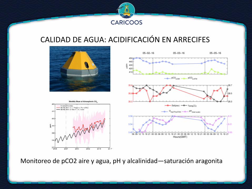
MonitoreodepCO2aireyagua,pHyalcalinidad—saturaciónaragonita

CALIDADDEAGUA:ACIDIFICACIÓNENARRECIFES

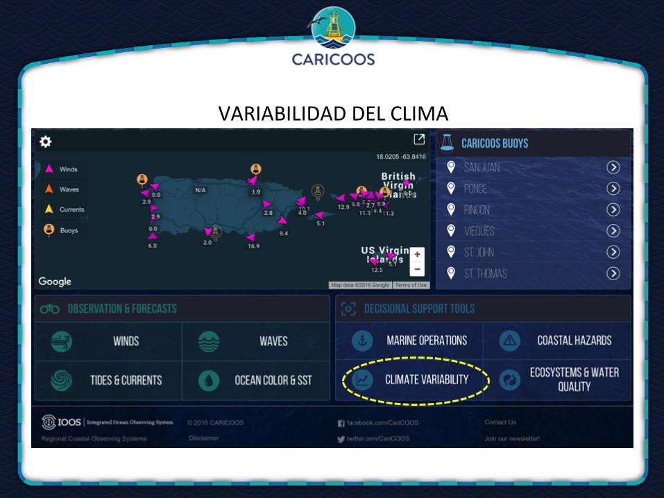
VARIABILIDADDELCLIMA

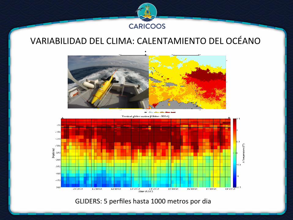
GLIDERS:5perfileshasta1000metrospordia

VARIABILIDADDELCLIMA:CALENTAMIENTODELOCÉANO:

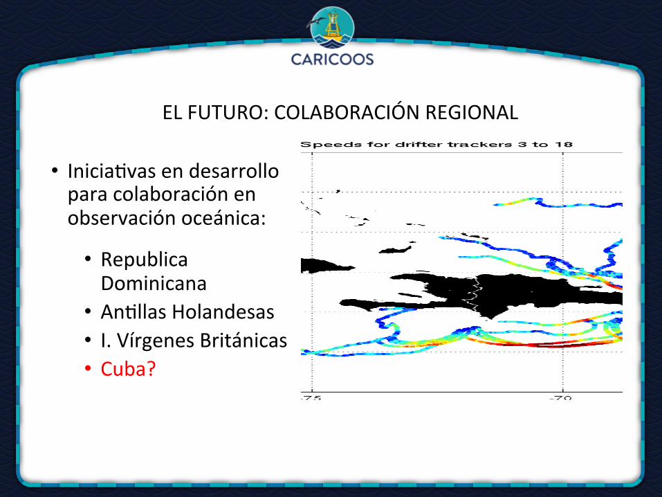
ELFUTURO:COLABORACIÓNREGIONAL

•  IniciaTvasendesarrolloparacolaboraciónenobservaciónoceánica:

•  RepublicaDominicana•  AnTllasHolandesas•  I.VírgenesBritánicas•  Cuba?