Journal of Agricultural and Resource Economics, 17(1): 205-217Copyright 1992 Western Agricultural Economics Association

Cash Forward Contracting versus Hedging ofFed Cattle, and the Impact of Cash Contracting onCash Prices

Emmett Elam

This research examines cash forward contracting of fed cattle. For an individual feeder,a cash contract eliminates basis risk (as compared to a futures hedge). However, thedisadvantage is that the contract price is estimated to be lower than the futures hedgeprice by $.28-$.59/cwt for steers and $.86-$1.64/cwt for heifers. From the industryperspective, contracting appears to have a negative impact on cash prices. An increaseof 1,000 head in U.S. monthly contract cattle shipments is associated with a $.003-$.009/cwt decrease in the U.S. average cash price. The negative impact of cash contractingvaries by state.

Key words: cash forward contract, fed cattle, futures hedge, risk.

A cash forward contract offers a means of fixing the price of fed cattle before they are ready for market.While cattle feeders are inclined to use cash contracts, they also recognize the potential negative impactof contracting on cash prices [National Cattlemen's Association (NCA); Ward and Bliss]. Some price-structure studies of livestock markets have concluded that the number of buyers is positively related toprice (Ward 1988). When packers forward contract cattle, they no longer need to buy these cattle in thecash market, reducing competition and possibly lowering cash prices. However, the hypothesis that thecash price of cattle will decrease as the number of buyers decreases is disputed by some who argue thatany diminished packer demand in the cash market as a result offorward contracting is offset by diminishedsupply in the cash market [U.S. General Accounting Office (U.S. GAO)]. Consequently, price should notbe impacted, either negatively or positively, as a result of increased cash contracting. Empirical evidenceis required to determine whether contracting impacts cash prices.

A study by Hayenga and O'Brien reports results from a regression model designed to measure theimpact of contracting on Colorado cash prices. The regression results show that an increase in the percentageof total slaughter contracted in Texas is associated with a significant decrease in the fed cattle price inColorado, whereas an increase in the contracting percentage in Kansas is associated with a significantincrease in the Colorado fed cattle price. Because of the different impacts of contracting on price, theauthors state that further analysis is needed before any conclusions can be drawn.

The concern about contracting is due to the increase in the number of contract cattle in recent years.Contracting, which was almost nonexistent before the early 1980s, became significant by the end of thedecade. From November 1988-May 1991, an average of 104,000 head of contract cattle were shippedper month in the four states of Colorado, Kansas, Nebraska, and Texas (Cattle-Fax). These four statesaccount for 90% of total contract shipments (Ward and Bliss). Survey results show that contract shipmentshave increased as a percentage of slaughter from 9% in 1986, to 14% in 1988, and 17% in 1989 [U.S.GAO; U.S. Department of Agriculture (USDA), News Division]. These percentages include marketingagreements plus cash contracts. This level of contracting potentially could have a negative impact on thecash market; however, the impact may differ depending on whether or not there is overcapacity in thepacking industry.

Emmett Elam is an associate professor in the Department of Agricultural Economics, Texas Tech University, Lubbock,Texas.

This is paper No. T-1-335, College of Agricultural Sciences, Texas Tech University.Appreciation is expressed to Don Ethridge, Sujit Roy, Charles Dodson, Jim Gill, and three anonymous reviewers

for their helpful comments on an earlier draft of this article.

205

Journal of Agricultural and Resource Economics

This research has two objectives. The first objective is to compare the futures hedge price and the cashforward contract price for fed cattle. Studies of grain and soybean markets show that the hedge price ishigher on average than the contract price (Harris and Miller for corn and soybeans in South Carolina;and Elam and Woodworth for soybeans in Arkansas). There is no published research that compares cashcontract and hedge prices for fed cattle; however, cattle feeders generally feel that the contract price islower than the hedge price (Stalcup; Ward and Bliss). Cash forward contract prices were obtained froma sample of cash contracts from six Texas feedlots and compared with the futures hedge price.

The second objective of this research is to determine whether cash contracting has a significant impacton the cash market price. Simple correlation coefficients are calculated between the amount of contractcattle shipments in a month and the cash price. Also, a price transmission equation is estimated whichrelates the fed cattle price to various economic variables, including a variable measuring the amount ofcash contracting. The sign and magnitude of the estimated contract coefficient measure the impact ofcontracting on the cash market. If contracting reduces competition in the cash market and causes the cashprice to be lower, then the estimated coefficient on the contract variable should be negative.

Cash Contracting versus Hedging

Fed cattle can be forward priced using a cash forward contract, which is an agreement by a cattle feederto deliver to a packer a specified number of cattle in a designated future month. Two types of contractsare available. A flat price contract specifies the price at the time the contract is signed by the cattle feederand packer. By contrast, a basis contract specifies the basis level (cash price minus futures price) at thetime the contract is signed, with the price left to be fixed at a later time. The feeder can fix the contractprice at any time prior to the month cattle are to be delivered to the packer. The contract price is determinedby adding the basis specified in the contract, which can be either positive or negative, to the futures priceon the day cattle are priced. A basis contract allows a feeder to fix the basis at one point in time, but waituntil sometime later to fix the price, perhaps after the price level has increased. The contract basis (orprice) is negotiated by the packer and the cattle feeder (or feedlot manager who represents the feeder'sinterests).

Cash contracts call for delivery of cattle to a specified packing plant, with the cattle feeder paying thecost of transportation (unless waived by the packer in some cases). A partial payment of $10 per head ismade to the cattle feeder at the time a cash contract is signed.1 Cash contracts can include specificationssuch as quality grade, yield grade, dressing percentage, etc., or the specifications may be waived. In non-spec contracts, the packer assumes the risk of quality and yield variation on the cattle.

An alternative means for pricing fed cattle is to hedge them with live cattle futures contracts traded onthe Chicago Mercantile Exchange. When the cattle reach their finished weight, they are placed on thefeedlot showlist and sold f.o.b. the feedlot to the highest bidder. Cattle are weighed at the feedlot and a4% pencil shrink is applied (as with contract cattle).

A cash contract has advantages and disadvantages compared with a hedge for pricing feedlot cattle(Elam and Woodworth; Hieronymus). One advantage of a cash contract is that an exact price can bedetermined. By contrast, only an approximate price is determined when a hedge is placed. With a cashforward contract, a cattle feeder is not required to deposit margin money as with a futures market hedge,or meet margin calls if the price should rise. Cattle feeders may gain benefits from lenders by using a cashcontract because basis risk and margin calls are eliminated. A forward contract can be used to price anynumber of cattle, rather than multiples of the 40,000 pound cattle futures contract. Also, a cash contractprovides a cash buyer for cattle in a concentrated market and avoids daily use of time spent negotiatinga price (NCA). By comparison, a hedger must locate a buyer and negotiate a price at the time the cattleare ready for market.2

The primary disadvantage of a cash contract, at least for grains and soybeans, is that the price is loweron average than the hedge price (Elam and Woodworth; Harris and Miller). This is because the contractingbuyer (elevator) is obliged to assume basis risk. To compensate, the grain elevator contracts with theproducer at a lower basis than he/she expected to exist at the time the grain (or soybeans) is to be delivered.

This research examines whether or not the cash contract price for fed cattle is lower than the hedgeprice. Fed cattle contracts were obtained from a sample of six feedlots in the Texas Panhandle, whichranged in capacity from 15,000-50,000 head. Three of the feedlots are located in the Texas Triangle(Canyon to Farwell to Plainview), while two lots are in the northern Panhandle, and one lot is in thesouthern Panhandle. One feedlot is in close proximity to the contracting packer's plant, whereas anotherlot is located a considerable distance from the plant. The six feedlots feed the usual types of cattle (notincluding Holsteins) that are typical of the Texas Panhandle. Contract prices from the six lots are comparedwith the futures hedge price over a two-and-one-half-year period.

206 July 1992

Fed Cattle Contracting 207

Hedge Price Compared with Contract Price

A fed cattle contract implicitly includes a basis if the contract is a fixed price contract, and explicitlyincludes a basis if it is a basis contract. The basis is for the nearby futures contract at the time the cattleare to be delivered (e.g., June futures for May cattle). When the cattle feeder decides to price the contractcattle, the contract price is determined by adding the contract basis to the futures price on that day. Bycomparison, the futures hedge price is determined by adding the futures sale price from the day the cattleare hedged, and the actual basis at the time the cattle are sold in the cash market.3

To remove the effect of varying price levels, it was assumed that a hedge was initiated at the same timethe contract price was fixed (i.e., with the futures price at a particular level). In the case of a basis contract,the basis can be set at one point in time (t), with the price left to be fixed at a later point (t + i). Incomparing a hedge and a cash contract, it was assumed that the hedge was initiated when the contractprice was fixed at time (t + i). Then the difference between the hedge and contract price is equal to thedifference between the hedge and contract basis figures. Because contract specifications call for cattle tobe delivered to the packing plant and hedge cattle are sold fo.b. the feedlot, and f because of the $10 perhead up-front payment on contract cattle, the raw basis figures had to be adjusted before comparisonscould be made.

The adjusted basis for a contract was obtained by taking the contract basis and (a) subtracting the costof transportation to the nearest packing plant and (b) adding the interest on the $10 per head up-frontdeposit:

(1) Adjusted Contract Basis = Contract Basis orac i- Cost of Transportation+ Interest on Deposit.

The figures in equation (1) are in dollars per hundredweight. The adjusted basis for a hedge was obtainedby subtracting the futures transaction costs from the actual basis at the time a hedge was lifted:(2) Adjusted Hedge Basis = Actual Basis - Transaction Costs.The futures transaction cost was assumed to be $. 125/cwt, i.e., the sum of a round-turn futures commissionof $.075/cwt ($30/400 cwt) plus an execution cost of $.05/cwt. The execution cost is the estimated costto enter and exit a futures position, i.e., the difference between the ask and bid prices (Hieronymus; Brorsenand Nielsen).

The adjusted hedge basis, adjusted contract basis, and the difference in the adjusted basis figures forTexas steers and heifers are shown in table 1. The adjusted contract basis figures were calculated from asample of non-spec cash contracts obtained from the six feedlots described above. The contracts from asmall sample of feedlots should be representative of contracts in the Panhandle, because contract bids ata given point in time are similar across packers and feedlots. A total of 274 steer contracts and 92 heifercontracts were collected, representing 57,459 head of steers and 16,250 head of heifers over the periodMay 1987 through September 1989. The truck mileage and cost to transport fed cattle from the feedlotto packing plant were obtained from the Texas Railroad Commission (regulated trucking rates, CommodityTariffs 8-M and 8-N). The cost to transport cattle varied depending on the tariff rate and the distancefrom feedlot to packing plant. Over the two-and-one-half-year study period, the average cost to transportcattle was $.40 per cwt. Three-month Treasury Bill rates were used to calculate the interest on the $10up-front deposit (Board of Governors of the Federal Reserve System). Contracts collected from the sixfeedlots typically did not include the date they were signed, and thus an assumption was made that acontract was held for four months.4

An adjusted hedge basis was calculated using the "average weighted cash price" for fed steers and heifersas reported by the Texas Cattle Feeders Association. Live cattle futures market prices were provided bythe Chicago Mercantile Exchange. It was assumed that Treasury Bills were used as margin for a futuresmarket position. Because Treasury Bills conjunctively earn interest as they serve as margin, on the averagethere is zero cost (no interest lost) on money deposited as margin for a futures market position.

The figures at the top of table 1 are monthly averages of the adjusted hedge and adjusted contract basisfigures for steers during the period May 1987 through September 1989. In eight of 12 months, the hedgebasis is higher than the contract basis. Across the 12 months of the year, the average hedge basis for steersis $.59/cwt higher than the average contract basis. The per-head difference is equal to $6.49 per head fora 1,100-pound steer over the two-and-one-half-year sample period. For heifers, the average differencebetween the adjusted hedge basis and adjusted contract basis figures is $1.64/cwt, or $16.40 per head fora 1,000-pound heifer. Monthly basis figures are not provided for heifers because of the smaller numberof heifer contracts in the data set.

The large difference between the hedge and contract basis figures for heifers compared with steers isdue in part to an increase in the cash price for heifers relative to steers during the study period. The

Elam

Journal of Agricultural and Resource Economics

Table 1. Average Adjusted Hedge Basis, Average Adjusted Con-tract Basis, and the Difference, Fed Steers and Heifers for the TexasHigh Plains, May 1987-September 1989

Sex and Average Adjusted BasisSex andDelivery Month Hedgea Contractb Difference

Steers: .............................................. $/cwt.Steers: --------------------------------------------- $/cwt ------------------------------------------January .42 -. 31 .73February -. 71 -. 10 -. 61March -. 42 -1.00 .58April .02 .11 -.09May 3.43 .06 3.37June 1.27 .02 1.25July 1.05 .28 .77August -. 10 .04 -. 14September -1.68 -.20 -1.48October -. 75 -.79 .04November .76 -. 43 1.19December 1.28 -.21 1.49Average, Jan.-Dec.c .38 -.21 .59

Heifers:Average, Jan.-Dec. -.55 -2.19 1.64

a Adjusted hedge basis = actual delivery month basis - futures transactioncosts [equation (1) in text].b Adjusted contract basis = contract basis - transportation cost + intereston deposit [equation (2) in text]. The contract basis was taken from cashforward contracts obtained from six Texas feedlots. The numbers of steercontracts used to calculate the average steer basis figures are: January, 29;February, 20; March, 13; April, 53; May, 32; June, 48; July, 15; August, 13;September, 14; October, 9; November, 13; December, 15. The total numberof steer contracts for all months is 274. The total number of heifer contractsused to calculate the average heifer basis (for all months) is 92.c Simple average of monthly figures.

increase was due to tight cattle supplies and packing plant overcapacity, and to a shift in consumer demandfor smaller retail cuts which are produced from heifer carcasses. As the cash price for heifers increasedrelative to that of steers, heifer feeders began to expect a higher contract basis for heifers. However, packerswere slow to increase the contract basis, despite the increase in the cash price/basis for heifers.

When comparing the hedge price to the forward contract price, an argument can be made for using anexpected basis in deriving the hedge price. An average of the historical basis over several years is oftenused as a proxy for the expected basis. The averaging process removes the influence of year-to-yearvariation which can cause the hedge price in a particular year to be high or low relative to the contractprice. The hedge price derived using the expected basis provides a more accurate indication of the trueprice that can be achieved from hedging. Because the difference between the hedge and contract prices issmall, it is particularly important to remove basis variation before making comparisons.

Because of the short sample period and the possibility for abnormal basis variation, hedge prices werecalculated using the expected basis. The average of the historical basis over a three-year period was usedas a proxy for the expected basis. For example, for a hedge to be lifted in May 1987, the three-year averageMay basis for the years 1984-86 was used as the expected basis for May 1987. Adjusted expected hedgebasis figures were calculated by subtracting the futures transaction costs from the expected (three-yearaverage) basis:

(3) Adjusted Expected Hedge Basis = Expected Basis - Transaction Costs.

The averages of the adjusted expected hedge basis figures for steers and heifers for the period May 1987through September 1989 are shown in column 2 of table 2. The adjusted hedge basis figures using theexpected basis are lower than the adjusted hedge basis figures using the actual basis (shown in table 1).This is due to an increase in the basis over the study period compared with the previous three years. Theamount the adjusted expected hedge basis is above the adjusted contract basis is $.28/cwt for steers and

208 July 1992

Fed Cattle Contracting 209

Table 2. Average Adjusted Expected Hedge Basis, Average Ad-justed Contract Basis, and the Difference, Fed Steers and Heifersfor the Texas High Plains, May 1987-September 1989

Average AverageAdjusted AdjustedExpected Contract

Sex Hedge Basisa Basisb Difference

........................................................-------------------- $/cwt ..........................................................Steers .07 -.21 .28Heifers -1.33 -2.19 .86

a Adjusted expected hedge basis = expected delivery month basis (three-yearaverage) - futures transaction costs [equation (3) in text].b Adjusted contract basis = contract basis - transportation cost + intereston deposit [equation (2) in text]. The contract basis was taken from cashforward contracts obtained from six Texas feedlots.

$.86/cwt for heifers, which is $3.08 per head for a 1,100-pound steer and $8.60 per head for a 1,000-pound heifer. These figures represent the per-head amount that the expected hedge price is above theactual contract price over the sample period.

Derived Risk Aversion Coefficients

One reason cattle feeders may choose to contract is because they prefer to eliminate the basis risk that ispresent when hedging. However, results of this study found that there is a cost for contracting; that is, acontract has a lower price on average than a hedge. The difference between the hedge price and the contractprice can be used to measure the risk aversion of cattle feeders. This difference is the insurance premiumthe cattle feeder implicitly pays for eliminating basis risk. For example, the insurance premium for steersfrom table 1 is $.59/cwt (which is the difference between the adjusted hedge basis and adjusted forwardcontract basis). The insurance premium is positively related to the risk aversion level of the cattle feeder.The more risk averse the cattle feeder, the higher the insurance premium the feeder is willing to pay toeliminate basis risk.

Pratt has shown that the insurance (risk) premium is equal to one-half the variance of the risk timesthe absolute risk aversion coefficient. In the present context, the insurance premium (IP) can be expressed as(4) IP = (MSE(N, - Ttj)r)/2,

where MSE(Nt - T,t_) is the average squared difference between the net and target prices from a hedge,and r is the Pratt-Arrow absolute risk aversion coefficient. The price risk in a cattle hedge is due to basisrisk, which causes the actual (net) price achieved from a hedge to differ from the target (expected) price.A detailed explanation of hedging risk is provided by Elam and Davis.

Equation (4) can be solved for the risk aversion coefficient:

(5) r = 2IP/MSE(N, - Tt,_).

This equation shows that risk aversion is equal to two times the insurance premium divided by thevariability of the risk. Using equation (5), the risk aversion coefficient for cattle feeders can be derivedbased on the IPs from tables 1 and 2 and an estimate of the MSE for a hedge. The estimated MSEs forthe period May 1987 through September 1989 are 1.70 for steers and 2.49 for heifers.5 The unit of measurefor the MSEs is dollars per cwt squared. Separate risk aversion coefficients were derived for steers andheifers, and for IP values based on the actual basis and expected basis (table 3). Because borrowed moneyfrequently is used to feed cattle, risk aversion coefficients were derived for leveraged cattle feeding.

The positive risk aversion coefficients in table 3 indicate that cattle feeders are averse to risk. This isevident from the fact that the forward contract price is lower than the hedge price (tables 1 and 2). Thederived risk aversion coefficients for heifer feeders are higher than those for steer feeders.

The estimated risk aversion coefficients in table 3 are higher than those typically reported in agriculturalresearch (Raskin and Cochran). For example, Holt and Brandt, in a study of hog hedging strategies, userisk aversion coefficients of .02-.04 for the category "risk averse" and .08-.10 for the category "highlyrisk averse." The derived risk aversion coefficients for unleveraged cattle feeders in table 3 are considerablyhigher than for hog feeders. In leveraged cattle feeding, risk increases because a given amount of moneycontrols a larger amount of assets (which increases the variability of the return). With an average of 25%

Elam

Journal of Agricultural and Resource Economics

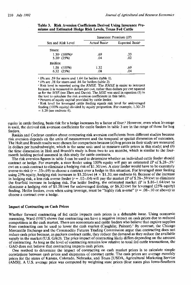
Table 3. Risk Aversion Coefficients Derived Using Insurance Pre-miums and Estimated Hedge Risk Levels, Texas Fed Cattle

Insurance Premium (IP)

Sex and Risk Level Actual Basisa Expected Basisb

Steers:1.30c (100%)d .69 .335.20e (25%) .04 .02

Heifers:1.58 (100%) 1.32 .696.32 (25%) .08 .04

a IPs are .59 for steers and 1.64 for heifers (table 1).b IPs are .28 for steers and .86 for heifers (table 2).c Risk level is reported using the RMSE. The RMSE is easier to interpretbecause it is measured in dollars per cwt, rather than dollars per cwt squaredas for the MSE (see Elam and Davis). The MSE was used in equation (5) inthe text to calculate the risk aversion coefficients in this table.d Percent of equity capital provided by cattle feeder.e Risk level for leveraged cattle feeding equals risk level for unleveragedfeeding (100% equity) divided by equity proportion. For example, 1.30/.25= 5.20 (see endnote 6).

equity in cattle feeding, basis risk for a hedge increases by a factor of four.6 However, even when leverageis used, the derived risk aversion coefficients for cattle feeders in table 3 are in the range of those for hogfeeders.

Raskin and Cochran caution about comparing risk aversion coefficients from different studies becauserisk aversion depends on the units of measurement and the temporal or spatial dimension of outcomes.The Holt and Brandt results were chosen for comparison because (a) hog prices in their study are measuredin dollars per hundredweight, which is the same unit used to measure cattle prices in this study; and (b)the time dimension in Holt and Brandt's study is from two to ten months, which is similar to the four-month holding period assumed in this study for cattle contracts.

The risk aversion figures in table 3 can be used to determine whether an individual cattle feeder shouldcontract or hedge. For example, a steer feeder using 100% equity will pay an estimated IP of $.28-.59/cwt on a cash contract to eliminate a hedging risk of $1.30/cwt. A steer feeder would have to be extremelyaverse to risk (r = .33-.69) to choose a contract over a hedge in this situation. For leveraged steer feedingusing 25% equity, hedging risk increases to $5.20/cwt (4 x $1.30; see endnote 6). Because of the increasein hedging risk, a less risk averse feeder (r = .02-.04) will pay the market IP of $.28-.59/cwt to eliminatethe fourfold increase in hedging risk. For heifer feeding, the estimated market IP is $.86-1.64/cwt toeliminate a hedging risk of $1.58/cwt for unleveraged feeding, or $6.32/cwt for leveraged (25% equity)feeding. Heifer feeders, even when using leverage, must be "highly risk averse" (r = .08-. 10 or above) tochoose a contract over a hedge.

Impact of Contracting on Cash Prices

Whether forward contracting of fed cattle impacts cash prices is a debatable issue. Using economicreasoning, Ward (1987) shows that contracting can have a negative impact on cash prices due to reducedcompetition in the cash market. There are economists and cattle feeders who believe that captive suppliesfrom contracting can be used to lower the cash market (Caughlin; Painter).7 By contrast, the ChicagoMercantile Exchange and the Commodity Futures Trading Commission argue that contracting does notreduce cash price because, as packers contract cattle, they reduce the demand as they reduce the availablesupply in the market (U.S. GAO). The price impact of contracting likely differs depending on the amountof contracting. As long as the level of contracting remains low relative to total fed cattle transactions, theGAO does not believe that contracting impacts cash prices.

One method to determine the impact of contracting on cash market prices is to calculate simplecorrelations between cash prices and shipments of contract cattle. The cash prices are average monthlyprices for the states of Kansas, Colorado, Nebraska, and Texas [USDA, Agricultural Marketing Service(AMS)]. A U.S. average price was computed by weighting state prices (four states plus Iowa-Southern

210 July 1992

Fed Cattle Contracting 211

Table 4. Simple Correlation Coefficients (r) between Fed CattleCash Price and Contract Shipments, Using Monthly Data for 1988-10 through 1991-05

Simple Correlation Coefficient (r)

Location Original Series First Differences

Kansas -.37ab -.18Colorado -. 54b -. 23bNebraska -.09 -.03Texas -.20 -.02U.S. -.36 b -. 11

Note: The number of observations for the original series is n = 32, exceptfor Nebraska where n = 31. The first-difference series has one less obser-vation.a Correlation coefficient between Kansas fed cattle prices and Kansas contractcattle shipments.b Significant at the .10 level using a one-tailed t-test.

Minnesota) by the proportion of commercial slaughter in each state. The Iowa-Southern Minnesota pricewas included to represent Midwest feeding. Cattle-Fax has reported monthly shipments of contract cattlein four states (mentioned above) since October 1988. The data are based on a survey of Cattle-Fax memberfeedyards (which account for more than one-half the marketings of fed cattle in the four states) and surveyinformation from other sources such as the Texas Cattle Feeders Association.

The estimated correlation coefficients between cash prices and contract shipments are negative for theU.S. and all four states (table 4). Correlations for the U.S., Kansas, and Colorado are significant at the.10 level for a one-tailed test.8 Negative correlations indicate that an increase in contract shipments isassociated with a decrease in the cash price. Also reported in table 4 are correlations between first differencesin prices and contract shipments. First differences are used to eliminate any trends in the variables. First-difference correlations are also negative for the U.S. and for each state individually.

Another means of determining whether contracting impacts cash prices is by estimating a price trans-mission equation-which can be derived from the demand and supply functions for marketing services(George and King; Tomek and Robinson). Marketing studies have estimated price transmission equationswhich relate the price at one level in the marketing channel to the price at another level (e.g., George andKing; Schultz and Marsh). Applied to this study, the price of fed cattle (the dependent variable at theslaughter level) is related to the price of wholesale beef. Other explanatory (independent) variables includedin the price transmission equation are (a) value of byproducts; (b) cost of marketing inputs (e.g., labor,materials, etc.); and (c) quantity of product being handled by the marketing system. A variable whichmeasures the amount of contracting can be added, and the estimated coefficient for this variable analyzedto determine the impact of contracting on cash prices. If contracting reduces competition in the cashmarket and causes the cash price to be lower, then the estimated coefficient on the contract variable shouldbe negative. By contrast, if contracting does not reduce competition, then the estimated coefficient shouldbe approximately zero.

A price transmission equation at the slaughter level can be specified as follows:

(6) PS, = A0 + [1PW, + f 2BP, + f3MC, + f 4Qt + P5CS, + Ut,

where PS = average price of Choice 1,100-1,300 pound steers, dollars per cwt (USDA, AMS); PW =wholesale price of beef (boxed value or carcass price), dollars per cwt; MC = index of marketing cost,1982 = 100 [simple average of Producer Price Index for materials (U.S. Department of Commerce) andindex of meat packer wages (U.S. Department of Labor)]; BP = beef byproduct allowance, dollars percwt (White et al.); Q = commercial beef production, millions of pounds (USDA, AMS); and CS = contractcattle shipments, 1,000s of head (Cattle-Fax). All variables in equation (6) are measured at time t. Thecoefficients, 0, .... , f5, are population coefficients, and ut is a random (non-autocorrelated, homoskedastic)error term with expected mean zero. 9 Small English letters are used to represent least squares estimatesof the population coefficients. The least squares coefficients b1 and b2 are expected to be positive. Thecoefficient b3 is expected to be negative because as marketing cost increases, the live animal price shoulddecrease relative to the wholesale price. The coefficient b4 is generally expected to be negative to reflecta higher margin associated with larger quantities handled by the marketing system (Schultz and Marsh;Ikerd; Breimyer).

Elam

Journal of Agricultural and Resource Economics

Table 5. Estimated Coefficients for U.S. Price Transmission Equations for Fed Steers Using MonthlyData

Explanatory VariablesBy- Mrkt. Com- Statistics

Wholesale Price/ Inter- Whl. product Cost mercial Contract StaDependent Variable cept Price Value Indexa Slaughter Shipmentsb R2 DWC

Boxed Cutout Value (n = 31):U'S. Price 34.59 .61 .42 -.35 -. 006 -. 004 .96 1.58

(3.54)d (15.60) (2.18) (-4.09) (-.77) (-1.19) e

U.S. Price w/Instr. Var. 39.60 .57 .67 -. 38 -. 001 -. 009 .83 1.53for Wholesale Price (2.11) (6.82) (1.80) (-2.19) (-.72) (- 1.52)

Carcass Price (n = 20):U.S. Price 33.69 .57 .81 -. 35 -. 000 -. 003 .98 2.09

(4.05) (17.18) (5.42) (-4.11) (.00) (-1.27)U.S. Price w/Instr. Var. 49.64 .54 1.24 -.61 .001 -. 007 .90 1.85

for Wholesale Price (2.52) (6.18) (3.70) (-3.29) (.76) (-1.10)

a Simple average of the Producer Price Index for intermediate materials (U.S. Department of Commerce) and meatpacker wage index (U.S. Department of Labor).b Number of contract cattle shipped per month in a state, in 1,000s of head (Cattle-Fax).c Durbin-Watson statistic. The equations were corrected for first-order autocorrelation.d Denotes t-value for testing the null hypothesis that the coefficient is zero.e Critical t-values for a one-tailed hypothesis test with 14 and 25 degrees of freedom are - 1.34 and - 1.32, respectively,for the. 10 significance level. The regressions using boxed cutout value included n = 31 observations, and the regressionsusing carcass price included n = 20 observations. The sample period is from November 1988 through May 1991.

Equation (6) was estimated using monthly data for the period October 1988 through May 1991. Thebeginning month of the estimation period was determined by the availability of contract shipments data.Equation (6) was estimated for individual states (Kansas, Colorado, Nebraska, and Texas) and the U.S.The U.S. results are shown in table 5. Separate equations were estimated using two series of wholesaleprices-boxed beef cutout value for Choice #2-3, 550-700 pound beef carcasses, and Choice #3, 600-800 pound steer carcasses. Carcass prices are available only through June 1990, because the USDAterminated carcass price reporting due to the small amount of carcass trade. Thus, only n = 21 observationswere used in estimating equation (6) when carcass price was used as the wholesale price. When boxedcutout value was used as the wholesale price, n = 32 observations were used in estimation (October 1988-May 1991).

An instrumental variable was used for PW because of the potential problem of correlation between PW(an endogenous variable in a meat sector model) and the error term (u) in equation (6). A two-stepprocedure was used where (a) the instrumental variable was developed from a regression of PW onexogenous variables such as beef production and income; and (b) the set of predicted values of wholesaleprices, PW, was used as the instrumental variable for PWin equation (6).10 The fact that PWis uncorrelatedwith the disturbance term in equation (6) guarantees that the least squares estimates are consistent.

The estimated coefficients b, b2, b3, and b4 are consistent with a priori expectations in all four estimatesof equation (6) (table 5). Equations were estimated using boxed beef cutout values and carcass price forwholesale prices, and an instrumental variable was used for the wholesale price, as well as the actualwholesale price. The estimated coefficients for PW and BP are positive and significant at the .10 level (orlower) in all four equations, and the coefficients for MC are negative and significant in all four equations.The estimated coefficients for Q are negative in three of the four equations, but are not significant.

The purpose for including a contract variable in equation (6) was to test rival conjectures regarding theimpact of contracting on cash prices. The null hypothesis tested is that contracting does not affect cashprices, i.e., Ho: /5 = 0 in equation (6). The alternative hypothesis is that contracting has a negative impacton price, i.e., Ha: f 5 < 0. A one-tailed test is used because there is no reason to expect that contractingcan increase cash prices.1

The estimated b5 values for contract shipments (-.003 to -. 009) are all negative for the U.S. regression(table 5). One of the estimated coefficients is significant at the .10 level and the other three coefficientsare significant at the .15 level. The estimated coefficients indicate that for each increase of 1,000 head ofcontract cattle shipped in a given month, the U.S. average cash price decreases by .30 to almost 1¢ percwt, ceteris paribus. The reader should be cautioned that the estimates are based on a small sample of n

212 July 1992

Fed Cattle Contracting 213

Table 6. Estimated Coefficients for State Price Transmission Equations for Fed Steers Using MonthlyData

Explanatory Variables

Wholesale Price/ By- Mrkt. State tDependent Whl. product Cost Commercial Contract StVariable Intercept Price Value Indexa Slaughter Shipmentsb R2 DWC

Boxed Cutout Value:Kansas Price 39.99 .57 .49 -.32 -. 010 -.037 .96 1.72

(5.77)d (20.02) (3.30) (-4.73) (-3.05) (-4.00)eColorado Price 40.86 .57 .43 -.38 -.006 -.018 .94 1.77

(3.37) (12.32) (1.93) (-3.91) (-.70) (-1.47)Nebraska Price 25.97 .65 .34 -.30 -.003 -. 004 .96 1.67

(3.12) (19.84) (1.96) (-3.60) (-.84) (-.36)Texas Price 35.67 .60 .50 -. 37 -. 003 -. 003 .94 1.49

(3.17) (14.10) (2.25) (-3.80) (-.68) (-.39)Carcass Price:

Kansas Price 40.45 .54 .97 -.40 -. 002 -.024 .97 2.48(3.93) (13.60) (5.76) (-4.06) (-.43) (-2.70)f

Colorado Price 42.87 .48 .99 -.34 -.020 -. 015 .98 2.14(4.62) (15.84) (7.31) (-4.44) (-2.61) (-1.42)

Nebraska Price 18.79 .62 .75 -.26 .001 -.003 .98 2.07(2.10) (19.14) (5.55) (-2.84) (.22) (-.33)

Texas Price 47.18 .52 .96 -.44 -.003 -.007 .88 1.95(3.99) (10.75) (4.31) (-3.95) (-.56) (-.91)

a Simple average of the Producer Price Index for intermediate materials (U.S. Department of Commerce) and meatpacker wage index (U.S. Department of Labor).b Number of contract cattle shipped per month in a state, in 1,000s of head (Cattle-Fax).c Durbin-Watson statistic. The equations were corrected for first-order autocorrelation.d Denotes t-value for testing the null hypothesis that the coefficient is zero.e Critical t-value for a one-tailed hypothesis test with 25 or 26 degrees of freedom is -1.32 for the .10 significancelevel. The regressions using boxed cutout value for Kansas, Colorado, and Texas included n = 32 observations, andthe regression for Nebraska included n = 31 observations.f Critical t-value for a one-tailed hypothesis test with 14 or 15 degrees of freedom is -1.34 for the .10 significancelevel. The regressions using carcass price for Kansas, Colorado, and Texas included n = 21 observations, and theregression for Nebraska included n = 20 observations.

= 32 or 21 observations. However, the fact that the estimated contract shipments coefficients in table 5are consistently negative for different estimation techniques (instrumental variable vs. noninstrumentalvariable), for different wholesale values (box vs. carcass), and for different time periods provides supportfor the conclusion that contracting has a negative impact on the cash price.' 2

A price change of less than 1 per cwt per 1,000 head seems small; however, it can make a substantialdifference in the return from feeding cattle if contract levels change by several thousand contracts. Anincrease of 10,000 head of contract cattle shipped in a month is associated with an estimated decrease of$.03-.09 per cwt in the fed cattle price, which is $.33 to $.99 per head for a 1,100-pound steer. Thisrepresents 3-9% (or more) of the average net return from feeding cattle-estimated at -$6.75 to +$10.65per head (Trapp and Webb; Trapp).

The estimates in table 5 are based on data for a period of overcapacity in the packing industry andrelatively tight supplies of cattle (NCA). The impact of contracting on cash prices may be different whensupplies increase (as they will over the course of the current cattle cycle).

The estimated impacts of contracting on individual state prices are shown in table 6. The estimates arebased on ordinary least squares using actual boxed cutout values and carcass price for the wholesale price(instrumental variables discussion follows). The estimated coefficients are consistent with a priori expec-tations. The signs of the coefficients are similar across states, except for the positive sign for the quantitycoefficient in the Nebraska equation with carcass price. The coefficients for contract cattle shipments arenegative in all equations. The coefficients are significant at the .10 level for Kansas and Colorado.

The estimated coefficients in table 6 indicate that the fed cattle price will decrease by $.02-.04/cwt inKansas and $.02/cwt in Colorado when contract cattle shipments increase by 1,000 head per month in a

Elam

Journal of Agricultural and Resource Economics

Table 7. Estimates for the Contract Shipments Coefficient Usingan Instrumental Variable for the Wholesale Price, by States

State Boxed Cutout Value Carcass Price

Kansas -. 046 (-2.24)a -. 021 (-1.14)bColorado -. 040 (-1.92) -.048 (-2.59)Nebraska -. 030 (-1.27) -.023 (-.96)Texas -. 009 (-.72) -.005 (-.33)

Note: The figures in this table are least squares estimates for the contractshipments coefficient, f5, in equation (6) in the text.a Critical t-value for a one-tailed hypothesis test with 25 or 26 degrees offreedom is -1.32 for the .10 significance level. The regressions using boxedcutout value for Kansas, Colorado, and Texas included n = 32 observations,and the regression for Nebraska included n = 31 observations. The sampleperiod is from October 1988 through May 1991.b Critical t-value for a one-tailed hypothesis test with 14 or 15 degrees offreedom is -1.34 for the .10 significance level. The regressions using carcassprice for Kansas, Colorado, and Texas included n = 21 observations, andthe regression for Nebraska included n = 20 observations.

state. The smallest negative impact of contracting is in Nebraska and Texas, where the estimated decreasein the fed cattle price is less than $.01/cwt for a 1,000-head increase in monthly contract cattle shipments.Texas and Nebraska account for the highest and lowest percentage of contract shipments, respectively,for the four states (i.e., 40% and 13%). The impact of contracting is also smallest for Texas for theinstrumental variable results discussed below. If monthly contract shipments in Texas were to increaseby 10,000 head, the Texas price of fed cattle would decrease an estimated 3-7¢ per cwt, or $.33-.77 perhead. By contrast, in Kansas if monthly contract cattle shipments increased by 10,000 head, the Kansasfed cattle price would decrease an estimated 24-37¢ per cwt, or $2.64-4.07 per head. Kansas contractsaccount for 27% of the four-state total contracts.

Equation (6) also was estimated for the four states using an instrumental variable for wholesale price.The estimated coefficients b,, b2, b3, and b4 are similar to the estimates obtained when using the actualwholesale price. The estimated coefficients for the contract shipments variable (bs) are shown in table 7for the instrumental variable regression. The two coefficient estimates for Colorado and one coefficientestimate for Kansas are significant at the .10 level. Compared to using the actual wholesale price (table6), the estimated coefficients are more negative for Colorado and Nebraska when an instrumental variableis used for the wholesale price.

Price flexibilities with respect to contract shipments are reported in table 8. A price flexibility measuresthe percentage of change in the fed cattle cash price for a 1% change in monthly contract shipments. Thesmallest price flexibilities (indicating the largest negative impact of contracting) are for Kansas and Col-

Table 8. Price Flexibilities with Respect to Contract Cattle Ship-ments

Colo- Nebras-Wholesale Price U.S. Kansas rado ka Texas

Actual Wholesale Price:Box Cutout Value -. 005 -. 013 -. 005 -. 001 -. 002Carcass -. 004 -. 009 -. 004 -. 001 -. 004

Instrumental Variable for Wholesale Price:Box Cutout Value -. 012 -. 015 -. 013 -. 005 -. 005Carcass -. 010 -. 008 -. 013 -. 004 -. 003

Note: Price flexibility is f = C5 (CS/PS), where #5 is the estimated slopecoefficient for the contract shipments variable (tables 5-7), and CS and PSare mean values of monthly contract shipments and cash steer prices, re-spectively. CS = 103.71, 27.84, 21.24, 13.03, and 41.57 for the U.S., Kansas,Colorado, Nebraska, and Texas, respectively; and PS = 76.55, 76.88, 76.59,76.55, and 76.76, respectively.

214 July 1992

Fed Cattle Contracting 215

orado. A price flexibility of -. 015 for Kansas indicates that a 1% increase in Kansas contract shipmentsis associated with a .015% decrease in the Kansas cash price. If Kansas contract shipments were to increaseby 50%, the Kansas cash price would decrease by .75%, which is $.58/cwt for cattle prices at the mean(i.e., .0075 x $76.88).

The price impact of contracting varies from state to state, possibly because of different numbers ofbuyers in each state. Colorado, for example, has only two major packers, whereas Nebraska has several. 13

The four-firm packer concentration ratio for Colorado is 99.9 compared to 72.3 for Nebraska (Ward1988). Consistent with the greater concentration in Colorado, the price flexibility with respect to contractshipments in Colorado is 2.6 times smaller than that for Nebraska (-.013 vs. -. 005, from table 8). Thedegree of concentration does not fully account for the different price impacts of contracting because Texasand Kansas have similar four-firm concentration ratios (84.7 and 88.4, respectively); however, the priceflexibility for Kansas is three times smaller than for Texas (-.015 vs. -. 005, from table 8). Further studyis needed to explain why contracting has different impacts in different states.

Summary and Conclusions

This research examined cash contracting of fed cattle from the viewpoint of both an individual feederand the industry. For an individual feeder, the primary disadvantage of a cash contract compared to afutures hedge is a lower price. Based on a sample of fed cattle contracts from six feedlots in Texas, it wasestimated that the contract price is lower than the hedge price by $.28-.59/cwt for steers and $.86-1.64/cwt for heifers. The difference between the hedge price and contract price represents the cost of eliminatingthe basis risk in a futures hedge. The relatively large estimated cost to contract suggests that cash contractswould be used by extremely risk averse cattle feeders. Notwithstanding the cost to contract, some cattlefeeders may choose a cash contract to eliminate basis risk and futures margin calls, and to guarantee acash buyer.

From an industry viewpoint, contracting appears to have a negative impact on cash prices. It is estimatedthat for each increase of 1,000 head of contract cattle shipments in a given month, the U.S. average cashprice of fed cattle will decrease by less than $.01/cwt. The negative impact of contracting varies by states.The greatest negative impact is in Kansas and Colorado where a 1,000-head increase in monthly contractshipments is associated with a $.02-.05/cwt decrease in the Kansas or Colorado price. The least negativeimpact is in Texas where a 1,000-head increase in monthly contract shipments is associated with a $.003-.009/cwt decrease in the Texas price.

[Received March 1991;final revision received December 1991.]

Notes

Partial payments of $10 per head were discontinued beginning in the summer of 1990.2 An alternative to a cash forward contract or futures hedge is to buy a put option on live cattle futures. A put option

does not eliminate basis risk, but it may be appealing to a risk averse hedger because it provides protection against adecline in price, without margin calls, and also allows the feeder to take advantage of higher prices.

3 The actual price for a short hedge is equal to the future price at the time the hedge is placed (F,_j) plus the actualbasis when the cattle are sold and the hedge is lifted (C, - F,), where C, and F, are the cash and futures prices,respectively, at the time the hedge is lifted [see equation (1) in Elam and Davis].

4 Ward and Bliss report that cattle feeders typically contract cattle two to four months prior to delivery to packers.The length of time a contract is held, however, has little effect on the comparison between contract and hedge pricesreported in this study. The only effect comes from the small amount of interest on the $10 up-front payment on contractcattle [which is added to the contract basis in equation (1) in the text].

5 Hedging risk was calculated using the following equation:

MSE(N, - T,) = - (B,- B)n ,=1

where B, is the average basis for the previous three-year period. For example, B, for January 1989 is the average ofthe January basis figures for 1986-88.

6 The risk level for leverage cattle feeding is:

Risk Level = [l/(Equity Proportion)]*Basis Riskfor Unleveraged Feeding.

This equation can be explained as follows. Assume that an unleveraged (100% equity) cattle feeder can make a returnof R dollars per cwt from feeding cattle. By using leverage, the cattle feeder increases the amount of cattle that can be

Elam

Journal of Agricultural and Resource Economics

fed with a given dollar investment. With a 25% equity investment, four times as many cattle can be fed, and thus thereturn increases to 4R. The variance of the return (or MSE) increases by a factor of 16 [i.e., var(4R) = 16var(R)],whereas the standard deviation (or RMSE) increases by a factor of four [i.e., std. dev.(4R) = 4 std. dev.(R].

7 A lower cash price could result if packers contract better quality cattle (i.e., quality and yield grade) and leave,perhaps, lower quality cattle in the cash market that will command a lower price anyway.

8 A one-tailed test was used because it was felt that contracting either has no impact on prices or a negative impacton prices. Thus, significant deviations from zero are expected to occur only in the negative direction.

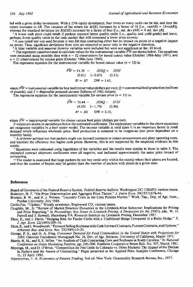
9 A time variable and seasonal dummy variables were included but were not significant at the .10 level.10 The regression equations used to calculate values for the instrumental variable PW are shown below. The equations

were estimated using monthly data with n = 32 observations for boxed cutout value (October 1988-May 1991), andn = 21 observations for carcass price (October 1988-June 1990).

The regression equation for the instrumental variable for boxed cutout value (n = 32) is:

PW= 11.28 - .002Q + .029I

(0.61) (-0.67) (5.51)

R2= .87 DW = 1.61,

where PW = instrumental variable for box beef cutout value (dollars per cwt); Q = commercial beef production (millionsof pounds); and I = disposable personal income (billions of 1982 dollars).

The regression equation for the instrumental variable for carcass price (n = 21) is:

PW = 70.44 - .009Q + .013I(4.05) (-1.79) (2.96)

R2 = .80 DW = 2.10,

where PW = instrumental variable for choice carcass beef price (dollars per cwt).T-values are shown in parentheses below the estimated coefficients. The explanatory variables in the above equations

are exogenous variables in a beef sector model. The income variable is used since it is an important factor in retaildemand which influences wholesale price. Beef production is assumed to be exogenous (not price dependent on amonthly basis).

' A reviewer pointed out that packers might use forward contracts to reduce procurement and plant operating costs,and translate the efficiency into higher cash prices. However, this is not supported by the empirical evidence in thisarticle.

12 Equations were estimated using logarithms of the variables and the results were similar to those in table 5. Theestimated contract shipment coefficients were all negative, and indicated approximately the same price impact ofcontracting.

13 The reader is cautioned that large packers do not buy cattle only within the state(s) where their plants are located,and thus the number of buyers may be greater than the number of packers with plants in a given state.

References

Board of Governors of the Federal Reserve System. Federal Reserve Bulletin. Washington DC: USGPO, various issues.Breimyer, H. F. "On Price Determination and Aggregate Price Theory." J. Farm Econ. 39(1957):678-94.Brorsen, B. W., and R. J. Nielsen. "Liquidity Costs in the Corn Futures Market." Work. Pap., Dep. of Agr. Econ.,

Purdue University, July 1986.Cattle-Fax. "Update." Weekly newsletter, Englewood CO, various issues.Caughlin, M., Jr. "Review of Market Structure Dynamics in the Livestock-Meat Subsector: Implications for Pricing

and Price Reporting." In Proceedings, Key Issues in Livestock Pricing: A Perspective for the 1990's, eds., W. D.Purcell and J. Rowsell. Blacksburg VA: Research Institute on Livestock Pricing, December 1987.

Elam, E., and J. Davis. "Hedging Risk for Feeder Cattle with a Traditional Hedge Compared to a Ratio Hedge." S.J. Agr. Econ. 22(1990):209-16.

Elam, E., and J. Woodworth. "Forward Selling Soybeans with Cash Forward Contracts, Futures Contracts, and Options."Arkansas Bus. and Econ. Rev. 22(1989): 10-20.

George, P. S., and G. A. King. Consumer Demand for Food Commodities in the United States with Projections for1980. Giannini Foundation Monograph No. 26, Div. of Agr. Sciences, University of California, March 1971.

Harris, H. M., and S. E. Miller. "An Analysis of Cash Contracting Corn and Soybeans in South Carolina." In NationalConference on Grain Marketing Patterns, pp. 290-300. Southern Cooperative Series Bull. No. 307, March 1981.

Hayenga, M., and D. O'Brien. "Competition for Fed Cattle in Colorado vs. Other Markets: The Impact of the Declinein Packers and the Ascent of Contracting." Paper presented at the Applied Price Analysis Conference, ChicagoIL, 23 April 1990.

Hieronymus, T. A. Economics of Futures Trading, 2nd ed. New York: Commodity Research Bureau, Inc., 1977.

216 July 1992

Fed Cattle Contracting 217

Holt, M. T., and J. A. Brandt. "Combining Price Forecasting with Hedging of Hogs: An Evaluation Using AlternativeMeasures of Risk." J. Futures Markets 5(1985):297-309.

Ikerd, J. E. Analysis of Farm to Retail Price Spreads to Improve Cattle Price Forecasts. Res. Bull. B-771, OklahomaState University, December 1983.

National Cattlemen's Association, NCA Beef Industry Concentration/Integration Task Force. Beef in a CompetitiveWorld. NCA Task Force Report, Denver CO, October 1989.

Painter, S. "Mounting a Challenge to the Powerful Packers." The Wichita Eagle, 22 April 1990, p. 2f.Pratt, J. W. "Risk Aversion in the Small and in the Large." Econometrica 32(1964):122-36.Raskin, R., and M. J. Cochran. "Interpretations and Transformations of Scale for Pratt-Arrow Absolute Risk Aversion

Coefficient: Implications for Generalized Stochastic Dominance." West. J. Agr. Econ. 11(1986):204-10.Schultz, R. W., and J. M. Marsh. "Steer and Heifer Price Differences in the Live Cattle and Carcass Markets." West.

J. Agr. Econ. 10(1985):77-92.Stalcup, L. "The Cost of a Forward Contract." Beef Today (February 1990):28-29.Texas Cattle Feeders Association. "Newsletter," various issues.Tomek, W. G., and K. L. Robinson. Agricultural Product Prices, 2nd ed. Ithaca NY: Cornell University Press, 1981.Trapp, J. N. "Seasonal Aspect of Cattle Feeding Profits." Current Farm Econ. 62(1989):19-30.Trapp, J. N., and J. K. Webb. "Cattle Feeding Profit Variances: Private Versus Public Data Comparisons." Current

Farm Econ. 59(1986):10-17.U.S. Department of Agriculture, Agricultural Marketing Service, Livestock Division. Livestock, Meat, and WoolMarket

News. Washington DC, various issues.U.S. Department of Agriculture, News Division, Office of Public Affairs. "USDA Program Announcements." Wash-

ington DC: USDA, 27 April 1990.U.S. Department of Commerce, Bureau of Economic Analysis. Survey of Current Business. Washington DC, various

issues.U.S. Department of Labor, Bureau of Labor Statistics. Employment and Earnings. Washington DC, various issues.U.S. General Accounting Office, Resources, Community, and Economic Development Division. Commodity Futures

Trading: Purpose, Use, Impact, and Regulation of Cattle Futures Markets. GAO/RCED No. 88-30, Report toCongressional Committees, November 1987.

Ward, C. E. "Market Structure Dynamics in the Livestock-Meat Subsector: Implications for Pricing and Price Re-porting." Proceedings, Key Issues in Livestock Pricing: A Perspective for the 1990's, eds., W. D. Purcell and J.Rowsell. Blacksburg VA: Research Institute on Livestock Pricing, December 1987.

. Meatpacker Competition and Pricing. Blacksburg VA: Research Institute on Livestock Pricing, July 1988.Ward, C. E., and T. J. Bliss. Forward Contracting of Fed Cattle: Extent, Benefits, Impacts, and Solutions. Res. Bull.

4-89, Research Institute on Livestock Pricing, Virginia Polytechnic Institute and State University, November1989.

White, T. F., Jr., L. A. Duewer, J. Ginzel, R. Bohall, and T. Crawford. Choice Beef Prices and Price Spreads Series:Methodology and Revisions. Staff Rep. No. AGES-9106, Commodity Economics Division, Economic ResearchService, USDA, Washington DC, February 1991.

Elam