Cash holdings, risk, and expected returns - …people.bu.edu/bpalazzo/Cash_Holdings.pdfCash holdings, risk, and expected returns† Dino Palazzo∗ November 3, 2011 Abstract In this

Cash holdings, risk, and expected returns †

Dino Palazzo∗

November 3, 2011

Abstract

In this paper I develop and empirically test a model that highlights how the correlation between cash flows

and a source of aggregate risk affects a firm’s optimal cash holding policy. In the model, riskier firms (i.e.,

firms with a higher correlation between cash flows and the aggregate shock) are more likely to use costly

external funding to finance their growth option exercises and have higher optimal savings. This precautionary

savings motive implies a positive relation between expected equity returns and cash holdings. In addition,

this positive relation is stronger for firms with less valuable growth options. Using a data set of US pubic

companies, I find evidence consistent with the model’s predictions.

Keywords: Expected equity returns, precautionary savings, growth options

JEL classification : G12, G32, D92

† I am very grateful to Gian Luca Clementi, Douglas Gale, Sydney Ludvigson, and Tom Sargent for their guidanceand encouragement. I also thank an anonymous referee, Rui Albuquerque, Francisco Barillas, Alberto Bisin, MichaelFaulkender (discussant), Jonathan Halket, Chuan-Yang Hwang, Matthias Kredler, Evgeny Lyanders, Cesare Robotti,Guido Ruta, Francesco Sangiorgi (discussant), Cecilia Parlatore Siritto, Stijn Van Nieuwerburgh, Gianluca Violante,Neng Wang, and the seminar participants at the New York University (NYU) Financial Economics Workshop, NYUMacro Student Lunch Seminar, Federal Reserve Bank of New York, NYU Stern Finance Seminar, Federal ReserveBank of Richmond, Federal Reserve Bank of New York, Boston University, Center for Monetary and Financial Studies(CEMFI), Instituto de Empresa, Pompeu Fabra University (UPF), Norwegian School of Economics and BusinessAdministration (NHH), Queen Mary University of London, Bocconi University, Tilburg University, University ofAmsterdam, Stockholm School of Economics, Bank of Italy, Federal Reserve Bank of Boston, 2009 Western FinanceAssociation (WFA) Conference, The Rimini Centre for Economic Analysis (RCEA) Money and Finance Workshop,University of North Carolina at Chapel Hill, and European Central Bank. I thank Lu Zhang for kindly providing thedata on the investment and profitability factors.

∗Department of Finance, Boston University School of Management, 595 Commonwealth Avenue, Boston, MA02215, United States. Email address: [email protected]. Tel.: +1 617 358 5872.

1. Introduction

This paper studies how the correlation between cash flows and a source of aggregate risk affects

the optimal cash holding policy of a firm. Using a three-period model of a firm’s investing and

financing decisions, I show how the riskiness of cash flows creates a novel motive for precautionary

savings that is incremental to those already identified in prior studies. This additional precautionary

savings motive allows me to explore the relation between cash holdings and equity returns and derive

testable implications, which I verify using data on US public companies.

The model presented here extends the three-period framework of Kim, Mauer, and Sherman

(1998) to allow for a source of aggregate risk. In my setup, a manager can finance investment

with retained earnings or equity. Equity issuance involves pecuniary costs, such as bankers’ and

lawyers’ fees, while savings allow the firm to avoid costly equity financing but earn a lower return

than shareholders could obtain outside of the firm. The optimal cash holding policy is pinned down

by the trade-off between the choice to distribute dividends in the current period or to save cash

and thus avoid costly external financing in the future. Unlike Kim, Mauer, and Sherman (1998), I

assume that investors are not risk-neutral. Specifically, shareholders value future cash flows using a

stochastic discount factor driven by a source of aggregate risk. As a result, riskier firms (i.e., firms

with a higher correlation between cash flows and the aggregate shock) have the highest hedging

needs because they are more likely to experience a cash flow shortfall in those states in which they

need external financing the most. Riskier firms’ optimal savings are therefore higher than those of

less risky firms.

This mechanism allows the model to produce a number of testable implications on the relation

between cash holdings and expected equity returns. First, an increase in the riskiness of cash flows

leads to an increase in both expected equity returns and retained earnings. In the data, a positive

correlation should be observed between cash holdings and equity returns. Second, the magnitude

of this correlation is larger for firms with less profitable investment opportunities. This prediction

stems from the fact that, in the model, firms with less profitable investment opportunities have

a smaller fraction of their total value tied to growth options and hence the expected return on

these firms’ assets in place has a larger weight in determining the overall expected return. As a

result, a change in the riskiness of the cash flows produced by a firm’s assets in place leads to a

2

larger change in expected returns the smaller is the profitability of the firm’s growth option. It

follows that two firms that differ only in their future investment profitability experience the same

increase in expected equity returns only if the firm with the more profitable investment opportunity

experiences a larger increase in riskiness. Given that a larger increase in riskiness also causes a

larger increase in cash holdings, a stronger marginal effect of expected equity returns should be

observed on cash holdings across firms with more profitable growth options.

To test the model’s predictions, I verify that an ex ante measure of expected returns has

a significant impact on corporate cash policies. Specifically, I follow the method proposed by

Gebhardt, Lee, and Swaminathan (2001) and modified by Wu and Zhang (2011) to construct an

accounting-based measure for expected equity returns. Using this measure, I test whether the

ex ante heterogeneity in expected equity returns is positively related to ex post differences in

cash holdings, as predicted by the model. This analysis complements other studies (e.g., Opler,

Pinkowitz, Stulz, and Williamson (1999)) that use cash flow volatility as a proxy for firm-level

risk. The results show that changes in cash holdings from one period to the next are positively

related to beginning-of-period expected equity returns. That is, firms with a higher expected equity

return experience a larger increase in their cash balance. This result is robust to the inclusion of

variables that control for expected cash flows and future investment opportunities, and it supports

the finding of a precautionary savings motive driven by expected equity returns.

In addition, to test if the relation between expected returns and cash holdings is influenced by

expected profitability, as predicted by the model, I run a subsample analysis using three different

measures for the profitability of a firm’s growth options. The results show that, when I use market

size and current profitability as proxies, firms with higher expected profitability have a larger

sensitivity of cash holdings to expected equity returns, thus confirming the model’s prediction.

When I use the third measure, the book-to-market ratio, the evidence is less favorable. This is

not a surprise given that the book-to-market ratio is a catch-all proxy for many variables, besides

future profitability.

In the second part of the empirical analysis, I perform a portfolio exercise in the spirit of Fama

and French (1993) to test whether cash holdings carry a positive risk premium. I first run a simple

portfolio sorting based on cash-to-asset ratios. This sorting is able to produce an equally weighted

excess return of the high cash-to-assets portfolio over the low cash-to-assets portfolio that on average

3

is positive and significant at 0.77% per month. When I use value-weighted returns, the excess return

is still positive with a point estimate of 0.41% per month, but it is not significant. However, when

I adjust for risk using the Fama and French (1993) or the Chen, Novy-Marx, and Zhang (2011)

three-factor models , the risk-adjusted excess return of the high cash-to-assets portfolio over the

low cash-to-assets portfolio is positive and significant both for equally and value-weighted excess

returns. Next, I perform three independent two-way sorts on cash holdings and the same proxies

for expected profitability used in the first part of the empirical analysis to verify that the cash

holdings–related excess return is larger for firms with less valuable growth options. I find that, for

equally weighted portfolios, the difference in the cash–related excess returns between high expected

profitability firms and low expected profitability firms is positive, significant, and varying between

0.54% and 1.28% per month. As in the one-way sort case, the results are less supportive when I use

value-weighted returns. In the latter case, the difference in the cash-related excess returns between

high and low expected profitability firms is positive and significant only when I use the book-to-

market ratio as a proxy. This leads to the conclusion that the evidence whether cash holdings carry

a positive risk premium based on realized equity returns is not as strong as the one produced using

the accounting-based measure for expected equity returns.

The model presented in this paper builds on the framework of Kim, Mauer, and Sherman (1998)

by introducing a source of aggregate risk. In this way, the link between corporate precautionary

savings and risk premia can be explicitly studied1. As in Kim, Mauer, and Sherman (1998), Gamba

and Triantis (2008) study the interaction between cash holdings and financing constraints in a setup

in which firms can both hoard cash and issue debt. They show that corporate liquidity is more

valuable for small and younger firms because it allows them to improve their financial flexibility.

They further show that combinations of debt and cash holdings that produce the same value of net

debt have a different impact on a firm’s financial flexibility. In a closely related model, Riddick and

Whited (2009) show that the firm’s propensity to save out of cash flows is negative and that cash

flow volatility is more important than financing constraints in shaping the optimal cash holdings

policy of a corporation.

1Other studies that provide a theory of optimal cash holdings are Huberman (1984), Almeida, Campello, andWeisbach (2004), Nikolov and Morellec (2009), Acharya, Almeida, and Campello (2007), Han and Qiu (2007),Asvanunt, Broadie, and Sundaseran (2010), Acharya, Davydenko, and Strebulaev (2011), and Bolton, Chen, andWang (2011).

4

These papers do not explicitly model the correlation of the firm’s cash flows with an aggregate

source of risk, and they do not study the link between the cross-section of equity returns and

capital structure decisions. Building on Berk, Green, and Naik (1999) and Zhang (2005), George

and Hwang (2010) and Gomes and Schmid (2010) propose two alternative models to rationalize the

negative relation between book leverage and average excess returns, but in their models cash can be

either distributed as dividends to shareholders or invested in new real assets. Livdan, Sapriza, and

Zhang (2009), in contrast, develop a model in which a manager can issue risk-free corporate debt

and save cash2. They show that the higher the shadow price of new debt, the lower the firm’s ability

to finance all the desired investments. As a result, the correlation of dividends with the business

cycle increases, leading to higher risk and higher expected returns. While Livdan, Sapriza, and

Zhang (2009) link risk premia to financing decisions, they do not study directly the determinants of

corporate precautionary savings and the role of this variable in shaping the cross-section of equity

returns.

The determinants of corporate cash holdings and their time-series properties have been widely

studied in the literature. Opler, Pinkowitz, Stulz, and Williamson (1999) show that for US public

companies the cash-to-asset ratio is negatively related to size and book-to-market and positively

related to capital expenditure, payouts, research and development expenditure, and cash flow volatility.

Consistent with Opler, Pinkowitz, Stulz, and Williamson (1999), Han and Qiu (2007) show that

the volatility of cash flows has a positive impact on a firm’s precautionary motive for holding cash;

this positive relation, however, is significant only for financially constrained firms. In this paper, I

explore the link between a firm’s cash holdings and its systematic risk (e.g., the correlation between

cash flows and an aggregate source of risk) instead of its cash flow volatility. In a related paper,

Simutin (2010) independently finds that firms with high excess cash holdings are more exposed to

systematic risk and earn a positive and significant excess return over firms with low excess cash

holdings3.

The outline of the paper is as follows. In Section 2, a simple financing problem in a three-period

framework shows how a precautionary savings motive can generate a positive correlation between

2? also study the interaction between the cost of equity and financing decisions, albeit in a model without debt.3In this paper, corporate cash holdings are identified using a firm’s cash-to-assets ratio. Other studies on the

determinants of cash holdings are Almeida, Campello, and Weisbach (2004), Dittmar and Mahrt-Smith (2007),Harford, Mansi, and Maxwell (2008), and Nikolov and Morellec (2009). Bates, Kahle, and Stulz (2009) provide anempirical analysis of the evolution of the cash-to-assets ratio for US public companies over the period 1980–2006.

5

cash holdings and expected equity returns. Section 3 contains the empirical analysis. Section 4

concludes.

2. Model

This section presents a model that departs from the risk-neutral setup of Kim, Mauer, and

Sherman (1998) by adding a stochastic discount factor and cash flows correlated with systematic

risk. In what follows, a firm expects an investment opportunity in the near future and needs to

decide whether to hoard cash, and thus earn a lower return than the opportunity cost of capital,

or to distribute dividends in the current period, and thus increase the expected cost of future

investment. This trade–off determines the current period’s optimal saving policy. The assumption

that cash flows are correlated with aggregate risk introduces an additional motive for precautionary

savings that drives riskier firms to save more, and this additional motive—absent in a risk-neutral

environment—is the key ingredient that generates a positive correlation between expected equity

returns and a firm’s cash holdings.

2.1. Setup

Consider a model, with periods indexed by t = 0, 1, 2. At time t = 0, a firm is endowed with

initial cash holdings equal to C0 and an asset (the risky asset) that produces a random cash flow

in period 1 only.

At time 1, after the realization of the risky asset’s cash flow, the firm has the option to install an

asset (the safe asset) that produces a deterministic cash flow (C2) at time t = 2 that is not pledgeable

at time t = 1. I assume that the investment opportunity arrives with probability π, π ∈ [0, 1], and

bears a fixed investment cost I = 1. If the firm has insufficient internal resources to pay for the

fixed cost, it can issue equity by paying a unit issuance cost equal to λ. The assumptions of a

stochastic cash flow and a fixed investment cost are made to generate the possibility of a liquidity

shock and a consequent need for external financing at time t = 1.

The firm can also transfer cash from one period to the next at the internal gross rate R̂ < R,

where R is the risk-free gross interest rate. Following Riddick and Whited (2009), an internal

6

w

t=0

Given the initial

cash endowment C0,

the firm decides to

transfer an amount

of cash S1 to the

next period.

w

t=1

The asset in place at

time 0 produces cash flows.

An investment opportunity

arrives with probability π.

A fixed cost I must be paid

if the firm invests.

w

t=2

Dividends are

distributed.

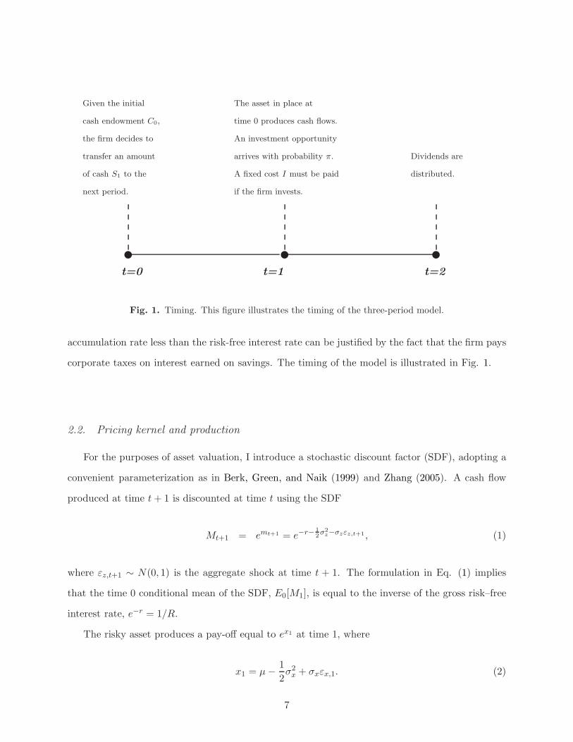
Fig. 1. Timing. This figure illustrates the timing of the three-period model.

accumulation rate less than the risk-free interest rate can be justified by the fact that the firm pays

corporate taxes on interest earned on savings. The timing of the model is illustrated in Fig. 1.

2.2. Pricing kernel and production

For the purposes of asset valuation, I introduce a stochastic discount factor (SDF), adopting a

convenient parameterization as in Berk, Green, and Naik (1999) and Zhang (2005). A cash flow

produced at time t + 1 is discounted at time t using the SDF

Mt+1 = emt+1 = e−r− 1

2σ2

z−σzεz,t+1, (1)

where εz,t+1 ∼ N(0, 1) is the aggregate shock at time t + 1. The formulation in Eq. (1) implies

that the time 0 conditional mean of the SDF, E0[M1], is equal to the inverse of the gross risk–free

interest rate, e−r = 1/R.

The risky asset produces a pay-off equal to ex1 at time 1, where

x1 = µ −1

2σ2

x + σxεx,1. (2)

7

The idiosyncratic shock, εx,1 ∼ N(0, 1), is correlated with the error term of the pricing kernel so that

the cash flows produced by the asset in place at time 0 are risky. I assume that COV (εz,1, εx,1) =

σx,z and, as a consequence, COV (x1,m1) = −σxσzσx,z = −βxm, where βxm is the systematic risk

of a project’s cash flow. Under the above assumptions, the time 0 value of the cash flow that will

be realized at time 1 is given by the certainty equivalent discounted at the (gross) risk–free interest

rate:

E0[em1ex1] = E0[e

−r− 1

2σ2

z−σzεz,1+µ− 1

2σ2

x+σxεx,1] = e−reµ−βxm. (3)

As βxm increases, the cash flow becomes more correlated with the aggregate shock and hence less

valuable.

2.3. The firm’s problem

At time 0, the firm has to decide how much of the initial cash endowment C0 to distribute as

dividends (D0) and how much to retain as savings (S1). Given that the return on internal savings

R̂ is lower than the risk-free rate R, S1 is always bounded above by C0.

To simplify the problem, I assume that the time 1 present discounted value of the safe project’s

cash flow, C2

R, is greater than the investment cost when the safe project is entirely equity-financed,

1 + λ. This condition is sufficient to ensure that the firm always invests at time 1 if an investment

opportunity arises. Conditional on investing at time 1, the firm issues equity only if corporate

savings, S1, plus the cash flow from the risky asset, ex1 , are not enough to pay for the investment

cost. In this case, the dividend at time 1, D1, is negative and the firm pays a proportional issuance

cost equal to λ. The last period’s dividend is the cash flow produced by the safe asset, D2 = C2.

If the firm does not invest at time 1, all the internal resources are distributed to shareholders and

the time 2 dividend is zero. The problem of the firm can be written as

V0 ≡ maxS1≥0

D0 + E0 [M1 (D1 + E1[M2D2])] , (4)

8

where

D0 = C0 −S1

R̂, (5)

D1 =

(1 + λχ1)(S1 + ex1 − 1) with probability π

S1 + ex1 with probability 1-π

, (6)

and

D2 =

C2 with probability π

0 with probability 1 − π

. (7)

χ1 is an indicator function that takes the value of one if the internal resources at time 1 are not

enough to pay for the fixed cost of investment (ex1 + S1 < 1), and M2 is the pricing kernel used in

period 1 to evaluate any pay-off in period 2. Proposition A.1, in Appendix A, provides a condition

for the existence and the uniqueness of an interior solution for the firm’s problem.

Assuming an interior solution, the optimal saving policy is such that the firm equates the cost

and the benefit of saving an extra unit of cash:

1 = R̂E0

[M1

]+ πλR̂E0

[M1χ1

]=

R̂

R+ πλR̂E0

[M1χ1

]. (8)

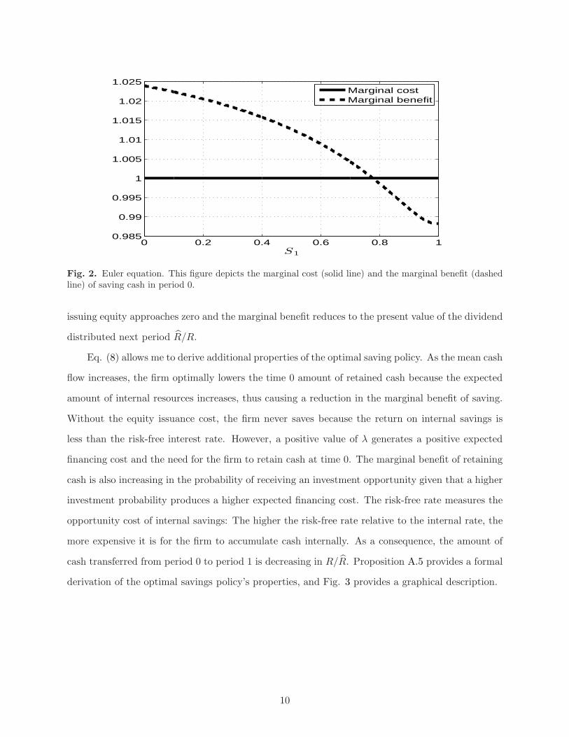
The marginal cost is simply one, the forgone dividend at time 0, and the marginal benefit is given

by the expected dividend that the firm will distribute next period plus the expected reduction in

equity issuance cost. The flat line in Fig. 2 reports the marginal cost of saving cash in period 0, and

the decreasing line is the marginal benefit. The latter is decreasing in S1 because the more cash a

firm saves, the smaller the probability of issuing equity in the future and the smaller the expected

reduction in equity issuance cost. If S1 approaches the fixed investment cost, the probability of

9

0 0.2 0.4 0.6 0.8 10.985

0.99

0.995

1

1.005

1.01

1.015

1.02

1.025

S1

Marginal costMarginal benefit

Fig. 2. Euler equation. This figure depicts the marginal cost (solid line) and the marginal benefit (dashedline) of saving cash in period 0.

issuing equity approaches zero and the marginal benefit reduces to the present value of the dividend

distributed next period R̂/R.

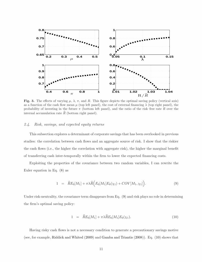
Eq. (8) allows me to derive additional properties of the optimal saving policy. As the mean cash

flow increases, the firm optimally lowers the time 0 amount of retained cash because the expected

amount of internal resources increases, thus causing a reduction in the marginal benefit of saving.

Without the equity issuance cost, the firm never saves because the return on internal savings is

less than the risk-free interest rate. However, a positive value of λ generates a positive expected

financing cost and the need for the firm to retain cash at time 0. The marginal benefit of retaining

cash is also increasing in the probability of receiving an investment opportunity given that a higher

investment probability produces a higher expected financing cost. The risk-free rate measures the

opportunity cost of internal savings: The higher the risk-free rate relative to the internal rate, the

more expensive it is for the firm to accumulate cash internally. As a consequence, the amount of

cash transferred from period 0 to period 1 is decreasing in R/R̂. Proposition A.5 provides a formal

derivation of the optimal savings policy’s properties, and Fig. 3 provides a graphical description.

10

0.2 0.3 0.4 0.50.65

0.7

0.75

0.8

µ0.05 0.1 0.15

0.4

0.6

0.8

1

λ

0.4 0.6 0.8 1

0.7

0.8

0.9

1

π1.01 1.02 1.03 1.040

0.2

0.4

0.6

0.8

R/R̂

Fig. 3. The effects of varying µ, λ, π, and R. This figure depicts the optimal saving policy (vertical axis)as a function of the cash flow mean µ (top left panel), the cost of external financing λ (top right panel), theprobability of investing in the future π (bottom left panel), and the ratio of the risk–free rate R over the

internal accumulation rate R̂ (bottom right panel).

2.4. Risk, savings, and expected equity returns

This subsection explores a determinant of corporate savings that has been overlooked in previous

studies: the correlation between cash flows and an aggregate source of risk. I show that the riskier

the cash flows (i.e., the higher the correlation with aggregate risk), the higher the marginal benefit

of transferring cash inter-temporally within the firm to lower the expected financing costs.

Exploiting the properties of the covariance between two random variables, I can rewrite the

Euler equation in Eq. (8) as

1 = R̂E0[M1] + πλR̂(E0[M1]E0(χ1) + COV [M1, χ1]

). (9)

Under risk-neutrality, the covariance term disappears from Eq. (9) and risk plays no role in determining

the firm’s optimal saving policy:

1 = R̂E0[M1] + πλR̂E0[M1]E0(χ1). (10)

Having risky cash flows is not a necessary condition to generate a precautionary savings motive

(see, for example, Riddick and Whited (2009) and Gamba and Triantis (2008)). Eq. (10) shows that

11

if the probability of investing next period is zero, then the firm will never retain cash because the

probability of issuing costly equity is also zero. However, the marginal benefit of retaining an extra

unit of cash is increasing in the probability of investing next period and hence the precautionary

motive is stronger in times when investment opportunities are likely to arise. The Euler equation

under risk-neutrality also reveals that firms with the same expected cash flows and the same probability

of investing next period will choose the same optimal savings policy given that they have the same

probability of issuing equity next period.

By contrast, Eq. (9) shows that firms with the same expected cash flows and the same probability

of investing next period will choose different savings policies depending on their cash flows’ correlation

with an aggregate shock. An increase in the covariance term will lower the expected value of firms’

cash flows in those future states in which the firm is more likely to issue equity (namely, when

the firm decides to invest and the realization of the aggregate shock is low). As a consequence, an

increase in riskiness leads to an increase in the time 1 expected financing cost, ceteris paribus, and

the firm reacts by increasing savings at time 0. This comparative static property is illustrated in

Panel A of Fig. 4 and formalized in Proposition A.2.

The expected return between time 0 and time 1 is the ratio of the time 0 expected future

dividends over the time 0 ex-dividend value of the firm P0:

E0[R0,1] =E0[D1 + P1]

P0=

E0[D1 + E1(M2D2)]

E0[M1 (D1 + E1[M2D2]). (11)

When the cash flows are uncorrelated with the stochastic discount factor, the expected equity

return is equal to the risk-free return R. When there is no investment opportunity (π = 0) or no

equity issuance cost (λ = 0), the optimal policy for the firm is to set S∗1 = 0. This will make the

expected equity return independent of the savings policy. These three cases are of no interest if the

focus is to study the relation between savings and expected equity returns. Hence, risk, a positive

expectation of future investment, and costly external financing are essential ingredients to explore

the link between cash holdings and equity returns.

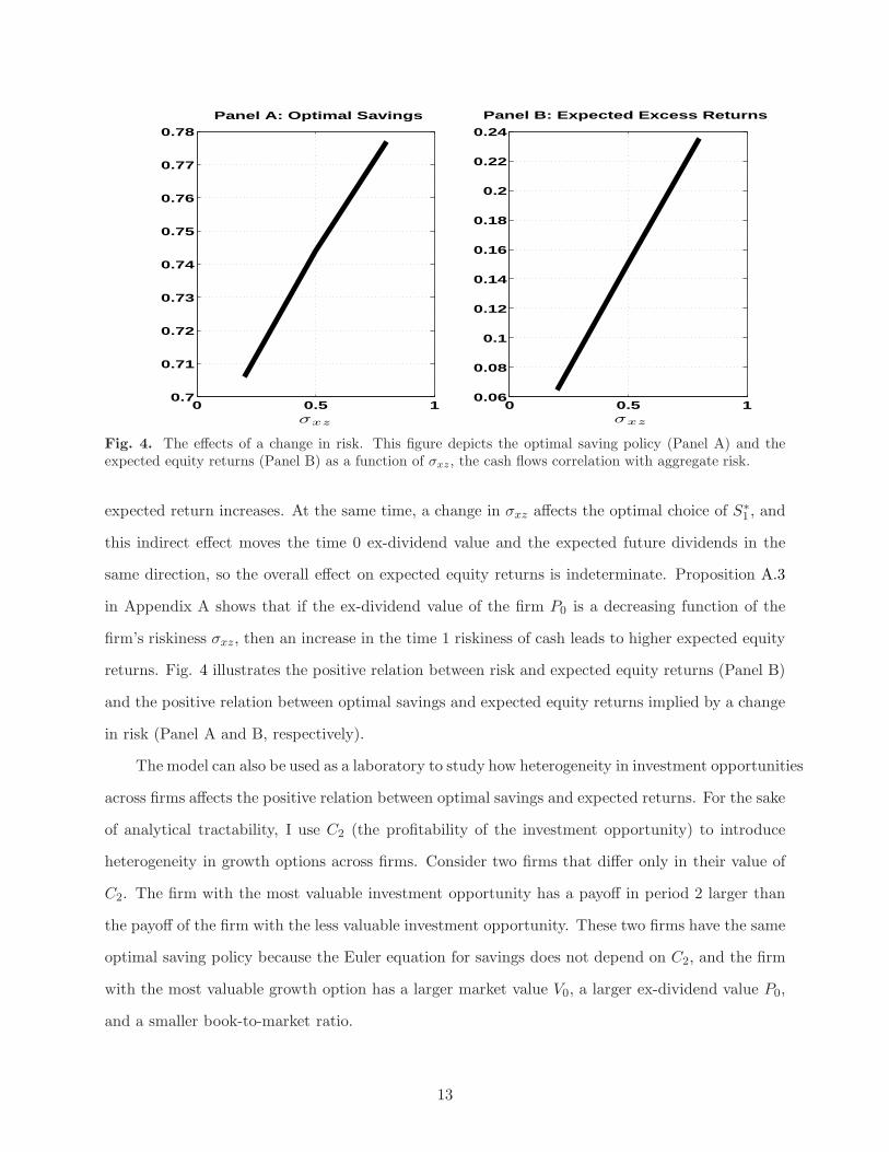
A change in the firm’s systematic risk affects expected returns through two channels. The

first channel works through the direct effect of a change in σxz. An increase in risk reduces the

time 0 ex-dividend value of the firm, while the expected future dividends are not affected. The

12

0 0.5 10.7

0.71

0.72

0.73

0.74

0.75

0.76

0.77

0.78

Panel A: Optimal Savings

σxz

0 0.5 10.06

0.08

0.1

0.12

0.14

0.16

0.18

0.2

0.22

0.24

Panel B: Expected Excess Returns

σxz

Fig. 4. The effects of a change in risk. This figure depicts the optimal saving policy (Panel A) and theexpected equity returns (Panel B) as a function of σxz, the cash flows correlation with aggregate risk.

expected return increases. At the same time, a change in σxz affects the optimal choice of S∗1 , and

this indirect effect moves the time 0 ex-dividend value and the expected future dividends in the

same direction, so the overall effect on expected equity returns is indeterminate. Proposition A.3

in Appendix A shows that if the ex-dividend value of the firm P0 is a decreasing function of the

firm’s riskiness σxz, then an increase in the time 1 riskiness of cash leads to higher expected equity

returns. Fig. 4 illustrates the positive relation between risk and expected equity returns (Panel B)

and the positive relation between optimal savings and expected equity returns implied by a change

in risk (Panel A and B, respectively).

The model can also be used as a laboratory to study how heterogeneity in investment opportunities

across firms affects the positive relation between optimal savings and expected returns. For the sake

of analytical tractability, I use C2 (the profitability of the investment opportunity) to introduce

heterogeneity in growth options across firms. Consider two firms that differ only in their value of

C2. The firm with the most valuable investment opportunity has a payoff in period 2 larger than

the payoff of the firm with the less valuable investment opportunity. These two firms have the same

optimal saving policy because the Euler equation for savings does not depend on C2, and the firm

with the most valuable growth option has a larger market value V0, a larger ex-dividend value P0,

and a smaller book-to-market ratio.

13

Given that the two firms share the same Euler equation for savings, a marginal increase in σxz

causes the same change in optimal savings for both of them. However, the expected equity return

depends on the value of C2 and, as Proposition A.4 shows, its sensitivity to a change in risk is

decreasing in the profitability of the future growth opportunity. This prediction stems from the

fact that firms with a smaller C2 have a smaller fraction of their value tied to the growth option

and hence the expected return on these firms’ assets in place is more important in determining

their overall expected return. As a result, a change in the riskiness of the cash flows produced by

a firm’s assets in place leads to a larger change in expected returns the smaller is the profitability

of the firm’s growth option. It follows that a change in riskiness causes the same change in savings

across the two firms, but a larger increase in expected return for the firm with the less valuable

growth option. Thus, the model predicts a stronger positive relation between cash holdings and

expected returns for firms with lower expected profitability.

2.5. Testable hypothesis

The model produces two testable hypotheses on the relation between corporate cash holdings

and expected equity returns.

Hypothesis 1 Expected equity returns and firm cash holdings are positively related because firms

with riskier assets in place are more likely to experience a cash flow shortfall when they are more

likely to issue equity.

Hypothesis 2 The magnitude of the positive relation between expected equity returns and firm

cash holdings depends on the profitability of future investment opportunities. The less profitable

the growth opportunities, the larger the change in expected equity returns associated with the same

change in cash holdings.

14

3. Cash holdings and the cross-section of equity returns: empirical

analysis

The empirical analysis consists of two parts. In Subsection 3.1, I investigate whether corporate

cash holding policies are driven by a firm-level measure of expected equity returns after controlling

for variables known to affect changes in the cash-to-assets ratio. In Subsection 3.2, I perform a

standard portfolio analysis in the spirit of Fama and French (1993). I first sort portfolios according

to their cash-to-asset ratio to test whether corporate cash holdings carry a positive risk premium,

and I then study whether the cash-related risk premium varies across firms that differ in terms of

their growth options’ profitability.

3.1. Cash holdings and expected equity returns

The model in Section 2 shows that heterogeneity in firms’ expected equity returns causes riskier

firms to hoard more cash to reduce expected financing costs (Hypothesis 1). In this subsection,

I test whether the variation in expected equity returns across firms is positively correlated with

changes in cash holding policies. As noted by Black (1993) and Elton (1999), among others, the

average realized equity return, used in standard portfolio analysis, is not a good proxy for expected

returns. I, therefore, follow a recent strand of the financial accounting literature that uses firm-level

data to construct accounting-based measures of expected equity returns. In particular, I rely on a

methodology known as the residual income model that allows one to evaluate an implied rate of

return (the proxy for expected equity returns) that equates the stock price of a company to the

present discounted value of future dividends, as described in Eq. (12)4:

Pt =∞∑

i=1

Et(Dt+i)

(1 + re)i, (12)

where Pt is the price of the stock at time t, Et(Dt+i) is the time t + i expected dividend, and re is

the internal rate of return, the proxy for the equity cost of capital. Appendix B provides a detailed

account of the methodology I adopt to derive the firm-level measure of expected equity returns.

4 Easton and Monahan (2005) provide a survey of the different accounting-based measures of expected equityreturns. The residual income model methodology used in this paper follows the work of Gebhardt, Lee, andSwaminathan (2001).

15

3.1.1. Cross–sectional regressions

In this subsection, I perform an exercise along the lines of Almeida, Campello, and Weisbach

(2004) by testing whether changes in corporate cash holdings can be explained by a firm’s expected

return, as measured by re, among other variables known to affect firms’ cash holding policies. Table

1 reports the results from the regression analysis. I exclude from the data set utilities [standard

industrial classification Code (SIC) codes between 4900 and 4949] and financial companies (SIC

codes between 6000 and 6999) because these sectors are subject to heavy regulation. The dependent

variable in all of the regressions is the change in the cash-to-assets ratio (∆CH) between years t−1,

and t and all the explanatory variables are truncated at the top and bottom 1% to limit the influence

of outliers. In the baseline regression, the set of explanatory variables includes the lagged value of

∆CH, which controls for cash holding policies’ mean reverting dynamics as suggested by Opler,

Pinkowitz, Stulz, and Williamson (1999), and the proxy for expected equity returns re evaluated at

time t−1. The pooled ordinary least squares regression (OLS) regression (Column 1) shows that the

coefficient on expected equity returns is positive and significant. A 0.10 increase in expected equity

returns is associated on average with a 0.01 change in the cash-to-assets ratio. The significance

of the coefficient on re does not disappear if I control for firm fixed effects (Column 4) or if I run

Fama and Macbeth regressions to control for time effects in corporate cash policies.

In Column 2 of Table 1, I add the lagged value of ∆CH and re to the baseline regression in

Almeida, Campello, and Weisbach (2004). CF is the cash flows-to-assets ratio, measured as the

ratio of income before extraordinary items (item IB in Compustat) over total assets at the end of

year t. BMt is the natural logarithm of book equity over market equity at the end of year t. As

in Davis, Fama, and French (2000), book equity is equal to stockholder equity (item SEQ), plus

balance sheet deferred taxes and investment tax credit (item TXDITC, if available), minus the

book value of preferred stock. In order of availability, preferred stock is equal to item PSTKRV, or

item PSTKL, or item PSTK. If item SEQ is missing, stockholder equity is equal to the book value

of common equity (item CEQ) plus the par value of preferred stock (item PSTKL). If item SEQ

and item CEQ are both missing, then stockholder equity is evaluated as total assets (item AT)

minus total liabilities (item LT). Market equity is the fiscal year end equity price (item PRCC F)

multiplied by the number of common shares outstanding (item CSHO). Size is the natural logarithm

16

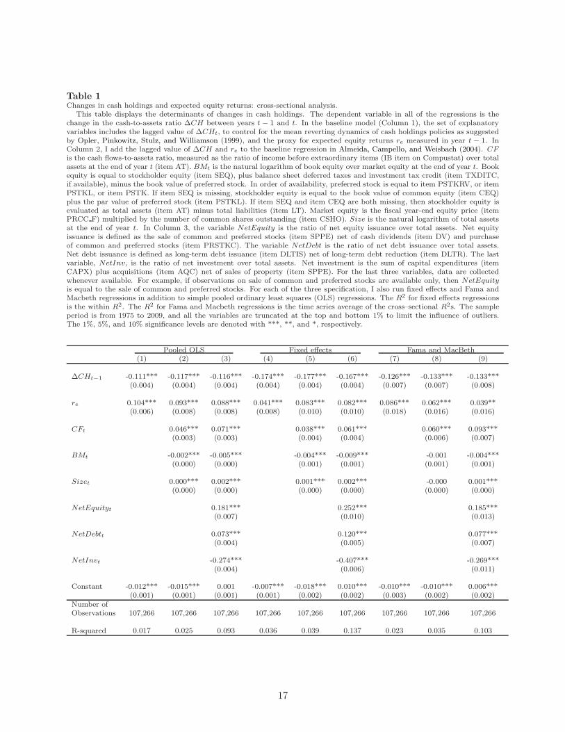
Table 1Changes in cash holdings and expected equity returns: cross-sectional analysis... This table displays the determinants of changes in cash holdings. The dependent variable in all of the regressions is thechange in the cash-to-assets ratio ∆CH between years t − 1 and t. In the baseline model (Column 1), the set of explanatoryvariables includes the lagged value of ∆CHt, to control for the mean reverting dynamics of cash holdings policies as suggestedby Opler, Pinkowitz, Stulz, and Williamson (1999), and the proxy for expected equity returns re measured in year t − 1. InColumn 2, I add the lagged value of ∆CH and re to the baseline regression in Almeida, Campello, and Weisbach (2004). CF

is the cash flows-to-assets ratio, measured as the ratio of income before extraordinary items (IB item on Compustat) over totalassets at the end of year t (item AT). BMt is the natural logarithm of book equity over market equity at the end of year t. Bookequity is equal to stockholder equity (item SEQ), plus balance sheet deferred taxes and investment tax credit (item TXDITC,if available), minus the book value of preferred stock. In order of availability, preferred stock is equal to item PSTKRV, or itemPSTKL, or item PSTK. If item SEQ is missing, stockholder equity is equal to the book value of common equity (item CEQ)plus the par value of preferred stock (item PSTKL). If item SEQ and item CEQ are both missing, then stockholder equity isevaluated as total assets (item AT) minus total liabilities (item LT). Market equity is the fiscal year-end equity price (itemPRCC F) multiplied by the number of common shares outstanding (item CSHO). Size is the natural logarithm of total assetsat the end of year t. In Column 3, the variable NetEquity is the ratio of net equity issuance over total assets. Net equityissuance is defined as the sale of common and preferred stocks (item SPPE) net of cash dividends (item DV) and purchaseof common and preferred stocks (item PRSTKC). The variable NetDebt is the ratio of net debt issuance over total assets.Net debt issuance is defined as long-term debt issuance (item DLTIS) net of long-term debt reduction (item DLTR). The lastvariable, NetInv, is the ratio of net investment over total assets. Net investment is the sum of capital expenditures (itemCAPX) plus acquisitions (item AQC) net of sales of property (item SPPE). For the last three variables, data are collectedwhenever available. For example, if observations on sale of common and preferred stocks are available only, then NetEquity

is equal to the sale of common and preferred stocks. For each of the three specification, I also run fixed effects and Fama andMacbeth regressions in addition to simple pooled ordinary least squares (OLS) regressions. The R2 for fixed effects regressionsis the within R2. The R2 for Fama and Macbeth regressions is the time series average of the cross–sectional R2s. The sampleperiod is from 1975 to 2009, and all the variables are truncated at the top and bottom 1% to limit the influence of outliers.The 1%, 5%, and 10% significance levels are denoted with ***, **, and *, respectively.

Pooled OLS Fixed effects Fama and MacBeth(1) (2) (3) (4) (5) (6) (7) (8) (9)

∆CHt−1 -0.111*** -0.117*** -0.116*** -0.174*** -0.177*** -0.167*** -0.126*** -0.133*** -0.133***(0.004) (0.004) (0.004) (0.004) (0.004) (0.004) (0.007) (0.007) (0.008)

re 0.104*** 0.093*** 0.088*** 0.041*** 0.083*** 0.082*** 0.086*** 0.062*** 0.039**(0.006) (0.008) (0.008) (0.008) (0.010) (0.010) (0.018) (0.016) (0.016)

CFt 0.046*** 0.071*** 0.038*** 0.061*** 0.060*** 0.093***(0.003) (0.003) (0.004) (0.004) (0.006) (0.007)

BMt -0.002*** -0.005*** -0.004*** -0.009*** -0.001 -0.004***(0.000) (0.000) (0.001) (0.001) (0.001) (0.001)

Sizet 0.000*** 0.002*** 0.001*** 0.002*** -0.000 0.001***(0.000) (0.000) (0.000) (0.000) (0.000) (0.000)

NetEquityt 0.181*** 0.252*** 0.185***(0.007) (0.010) (0.013)

NetDebtt 0.073*** 0.120*** 0.077***(0.004) (0.005) (0.007)

NetInvt -0.274*** -0.407*** -0.269***(0.004) (0.006) (0.011)

Constant -0.012*** -0.015*** 0.001 -0.007*** -0.018*** 0.010*** -0.010*** -0.010*** 0.006***(0.001) (0.001) (0.001) (0.001) (0.002) (0.002) (0.003) (0.002) (0.002)

Number ofObservations 107,266 107,266 107,266 107,266 107,266 107,266 107,266 107,266 107,266

R-squared 0.017 0.025 0.093 0.036 0.039 0.137 0.023 0.035 0.103

17

of total assets at the end of year t.

Table 1 shows that the cash flow sensitivity of cash (i.e., the coefficient on CF ) is positive and

significant over the entire sample in all of the regression specifications. In the pooled OLS case,

a 0.10 increase in the cash flows-to-assets ratio is associated on average with an increase in the

cash-to-assets ratio between 0.005 and 0.007. The sign of the coefficient on BM is in line with

the findings in Almeida, Campello, and Weisbach (2004). A higher BM signals lower investment

opportunities and is associated with a decrease in cash holdings. However, the significance is lost

in one case when I run Fama and Macbeth regressions (Regression 8). The coefficient on Size

is positive, and it is not significant only in the Fama and Macbeth regressions (Regression 8).

Controlling for cash flows, investment opportunities, and physical size does not affect the sign and

significance of the coefficient on re.

As a last robustness check, I test whether the uses and sources of funds from financing and

investing operations between t−1 and t have any effect on the positive correlation between expected

equity returns and changes in cash holdings (Column 3). The variable NetEquity is the ratio of net

equity issuance over total assets. I measure net equity issuance as the sale of common and preferred

stocks (item SPPE) net of cash dividends (item DV) and the purchase of common and preferred

stocks (item PRSTKC). The variable NetDebt is the ratio of net debt issuance over total assets,

where net debt issuance is defined as long–term debt issuance (item DLTIS) net of long–term debt

reduction (item DLTR). The last variable, NetInv, is the ratio of net investment over total assets.

Net investment is the sum of capital expenditures (item CAPX) plus acquisitions (item AQC) net

of sales of property (item SPPE)5.

The coefficients on the three variables have the expected sign and are always significant. An

increase in external financing (NetEquity and NetDebt) between t − 1 and t contributes to an

increase in the liquid resources held by the firm at the end of period t. An increase in investing

activity is associated with a reduction in the cash-to-assets ratio. Controlling for uses and sources

of funds between time t − 1 and t helps improve the degree to which cash holding changes can be

explained—the R2 more than doubles— but the sign and statistical significance of the proxy for

expected equity returns are not affected.

5For all of the variables, I collect the data whenever available. For example, if I have only observations on the saleof common and preferred stock, then NetEquity is equal to the sale of common and preferred stock.

18

3.1.2. Subsample analysis

In this subsection, I explore how future profitability affects the coefficient on expected equity

returns. According to the model, expected equity returns of firms with more valuable growth

options are less sensitive to a change in the riskiness of assets in place (Hypothesis 2). As a

consequence, two firms that differ only in their future investment profitability experience the same

increase in expected equity returns only if the firm with the more profitable investment opportunity

experiences a larger increase in riskiness. Given that a larger increase in riskiness also causes a

larger increase in cash holdings, a stronger marginal effect of expected equity returns should be

observed on cash holdings across firms with more profitable growth options.

The model also predicts that an increase in future profitability causes an increase the firm’s

market value and a corresponding decrease in the book-to-market ratio. It follows that size and

book-to-market are two natural proxies that one can use to measure future profitability. However,

these two variables, being a function of a firm’s market price, are at best a noisy proxy and for this

reason I also include the return on equity (ROE) as an additional measure of expected profitability6.

I sort firms according to their expected profitability following three schemes. First, I divide

firms into two size categories using the firm’s market capitalization in period t − 1: small firms

(firms in the bottom 30% of the size distribution) and large firms (firms in the top 30% of the size

distribution). Then, I sort firms into two book-to-market categories: small book-to–market firms

(firms in the bottom 30% of the book-to-market distribution) and large book-to-market firms (firms

in the top 30% of the book-to-market distribution). Finally, I sort firms into two ROE categories:

small ROE firms (firms in the bottom 30% of the ROE distribution) and large ROE firms (firms

in the top 30% of ROE distribution). Market capitalization and the book-to-market ratio are

measured as described in Subsection 3.1.1, and ROE is the ratio of income before extraordinary

items (item IB in Compustat) over the one-period lagged book value of equity, also defined in

Subsection 3.1.1. The sorting is performed at an annual frequency, and I use the one-period lagged

value of the market capitalization, book-to-market ratio, and ROE to align their timing with the

6Current profitability, as measured by the return on equity, is a highly persistent variable and for this reason itcan be considered a good measure of expected profitability.

19

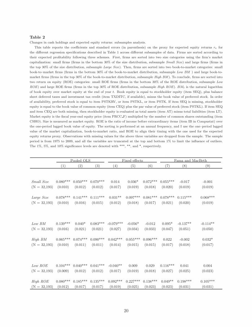
Table 2

Changes in cash holdings and expected equity returns: subsamples analysis.

.. This table reports the coefficients and standard errors (in parenthesis) on the proxy for expected equity returns re for

the different regression specifications described in Table 1 across different subsamples of data. Firms are sorted according to

their expected profitability following three schemes. First, firms are sorted into two size categories using the firm’s market

capitalization: small firms (firms in the bottom 30% of the size distribution, subsample Small Size) and large firms (firms in

the top 30% of the size distribution, subsample Large Size). Then, firms are sorted into two book-to-market categories: small

book-to–market firms (firms in the bottom 30% of the book-to-market distribution, subsample Low BM ) and large book-to-

market firms (firms in the top 30% of the book-to-market distribution, subsample High BM ). To conclude, firms are sorted into

two return on equity (ROE) categories: small ROE firms (firms in the bottom 30% of the ROE distribution, subsample Low

ROE) and large ROE firms (firms in the top 30% of ROE distribution, subsample High ROE). BMt is the natural logarithm

of book equity over market equity at the end of year t. Book equity is equal to stockholder equity (item SEQ), plus balance

sheet deferred taxes and investment tax credit (item TXDITC, if available), minus the book value of preferred stock. In order

of availability, preferred stock is equal to item PSTKRV, or item PSTKL, or item PSTK. If item SEQ is missing, stockholder

equity is equal to the book value of common equity (item CEQ) plus the par value of preferred stock (item PSTKL). If item SEQ

and item CEQ are both missing, then stockholder equity is evaluated as total assets (item AT) minus total liabilities (item LT).

Market equity is the fiscal year-end equity price (item PRCC F) multiplied by the number of common shares outstanding (item

CSHO). Size is measured as market equity. ROE is the ratio of income before extraordinary items (item IB in Compustat) over

the one-period lagged book value of equity. The sorting is performed at an annual frequency, and I use the one–period lagged

value of the market capitalization, book-to-market ratio, and ROE to align their timing with the one used for the expected

equity returns proxy. Observations with missing values for the above three variables are dropped from the sample. The sample

period is from 1975 to 2009, and all the variables are truncated at the top and bottom 1% to limit the influence of outliers.

The 1%, 5%, and 10% significance levels are denoted with ***, **, and *, respectively.

Pooled OLS Fixed effects Fama and MacBeth

(1) (2) (3) (4) (5) (6) (7) (8) (9)

Small Size 0.080*** 0.050*** 0.070*** 0.014 0.036* 0.072*** 0.055*** -0.017 -0.001

(N = 32,193) (0.010) (0.012) (0.012) (0.017) (0.019) (0.018) (0.020) (0.019) (0.019)

Large Size 0.078*** 0.141*** 0.111*** 0.031** 0.097*** 0.081*** 0.078*** 0.115*** 0.068***

(N = 32,193) (0.010) (0.016) (0.015) (0.012) (0.018) (0.017) (0.021) (0.020) (0.019)

Low BM 0.139*** 0.040* 0.083*** -0.079*** -0.056* -0.012 0.095* -0.137** -0.114**

(N = 32,193) (0.016) (0.021) (0.021) (0.027) (0.034) (0.033) (0.047) (0.051) (0.050)

High BM 0.065*** 0.074*** 0.090*** 0.042*** 0.055*** 0.096*** 0.022 -0.002 0.032*

(N = 32,193) (0.010) (0.011) (0.011) (0.014) (0.015) (0.015) (0.017) (0.018) (0.017)

Low ROE 0.104*** 0.040*** 0.041*** -0.040** 0.009 0.029 0.116*** 0.041 0.004

(N = 32,193) (0.009) (0.012) (0.012) (0.017) (0.019) (0.018) (0.027) (0.025) (0.023)

High ROE 0.080*** 0.185*** 0.135*** 0.092*** 0.227*** 0.138*** 0.049** 0.198*** 0.105***

(N = 32,193) (0.012) (0.017) (0.017) (0.019) (0.025) (0.023) (0.023) (0.031) (0.031)

20

one I use for the expected equity returns proxy. Observations with missing values for the three

variables are dropped from the sample.

Table 2 reports the coefficient on the expected equity return for the different book-to-market,

size, and ROE categories. When I use book-to-market to measure expected profitability, the results

are in line with what would expected only when pooled OLS regressions are considered. In this

case, the coefficients on the proxy for the expected equity return are always positive and, in one

case, low book-to-market firms have a coefficient larger and more than two standard errors away

from the estimated value for high book-to-market firms (Regression 1). The empirical results are

more supportive of the model’s prediction when expected profitability is measured using size or

ROE as proxies. In the former case, the estimated sensitivity of cash holdings to a change in

expected equity returns for small firms is smaller and more than two standard errors away from the

estimated value for large firms in five cases (Regressions 2, 3, 5, 8, and 9). In the latter case, the

estimated sensitivity of cash holdings to a change in expected equity returns for low ROE firms is

smaller and more than two standard errors away from the estimated value for high ROE firms in

seven cases (Regressions 2, 3, 4, 5, 6, 8, and 9).

Overall, the empirical analysis performed using an accounting-based proxy for expected equity

returns produces results consistent with the model’s predictions. First, an increase in the proposed

measure for expected equity returns is associated with an increase in cash holdings. Second, the

data also show support for the hypothesis that the marginal effect of expected equity returns on

cash holdings should be stronger across firms with more profitable growth options when size and

ROE are used as proxies for expected profitability.

3.2. Portfolio analysis

In this subsection, I perform a standard portfolio analysis in the spirit of Fama and French

(1993) that uses realized returns instead of expected returns. I first sort portfolios according to

their cash-to-asset ratio to test whether corporate cash holdings carry a positive risk premium

(Hypothesis 1), and I then study whether the cash-related risk premium varies across firms that

differ in terms of their growth options’ profitability (Hypothesis 2).

21

3.2.1. Data

Stock prices and quantities come from the Center for Research in Securities Prices (CRSP)

and accounting data come from Compustat Quarterly. To begin, I match the companies in CRSP

with companies in Compustat that have the same value for the security identifier PERMNO. I

then eliminate observations for which the first six digits of the Compustat Committee on Uniform

Security Identification Procedures (CUSIP) code differ from the first six digits of the CRSP CUSIP

code or the CRSP name CUSIP (NCUSIP) code.

I consider only ordinary common shares (share codes 10 and 11 in CRSP), and I exclude

observations related to suspended, halted, or non listed shares (exchange codes lower than 1 and

higher than 3). I also require that a stock has reported returns for at least 24 months prior to

portfolio formation. If a stock undergoes a performance delist after portfolio formation and the

delisting return is missing, I follow Shumway (1997) and assign to the missing equity returns a

value of -30%7.

A stock’s market value (Size) is defined as the value of the firm’s market capitalization at

portfolio formation. The monthly risk-free interest rate and the observations for the Fama and

French and momentum factors are taken from Kenneth French’s website8.

As in Subsection 3.1.1, I use the SIC code in Compustat to exclude from the data set utilities

(SIC codes between 4900 and 4949) and financial companies (SIC codes between 6000 and 6999)

because these sectors are subject to heavy regulation. I construct the book-to-market ratio (BM)

by dividing the book value of equity by the market value of equity at portfolio formation. Following

Chen, Novy-Marx, and Zhang (2011), the book value is equal to the book value of shareholders

equity, plus balance sheet deferred taxes and investment tax credits (item TXDITCQ, if available),

minus the book value of preferred stock. Shareholder equity is measured using stockholders’ equity

(item SEQQ). If the variable is not available, I use common equity (item CEQQ) plus the carrying

value of preferred stock (item PSTKQ). If both shareholder equity and common equity are missing,

I use total assets (item ATQ) minus total liabilities (item LTQ). The book value of preferred stock

is measured using the redemption value (item PSTKRQ, if available). If the quantity is missing,

I use the carrying value (item PSTKQ, if available). The cash-to-assets ratio (CH) is defined as

7The CRSP codes for poor performance delists can be found in the CRSP Delisting Returns guide, athttp://www.crsp.com/crsp/resources/papers/crsp_white_paper_delist_returns.pdf.

8 http://mba.tuck.dartmouth.edu/pages/faculty/ken.french/data_library.html.

22

http://www.crsp.com/crsp/resources/papers/crsp_white_paper_delist_returns.pdf

http://mba.tuck.dartmouth.edu/pages/faculty/ken.french/data_library.html

the value of corporate cash holdings (item CHEQ) over the value of the firm’s total assets (item

ATQ). The return on equity is the ratio of income before extraordinary items (item IBQ) over the

one–quarter–lagged book value of equity. Companies with a negative book-to-market ratio or a

negative cash-to-assets ratio are excluded from the sample. I use the quarterly accounting data

available in month t in portfolios sorts starting at time t + i + 1 if there has been an earnings

announcement (item RDQ) in month t + i, where i = 1, 2, 39.

3.2.2. One-way sorts

I start the portfolio analysis by sorting firms according to their cash-to-assets ratio using ten

deciles containing on average 248 firms. Following the strategy that Chen, Novy-Marx, and Zhang

(2011) use to construct their return on assets (ROA) factor (a cash-related variable), I rebalance

portfolios at a monthly frequency starting at the beginning of July 1972 and ending in December

2009, and I assume a one-month holding period. Table 3 reports the time series average of the cross-

sectional mean and median values for the book-to-market, market size, net assets, profitability, and

post-ranking βs across the ten portfolios. The book-to-market ratio is used as a proxy for future

investment opportunities (growth options). Net assets (defined as total assets net of cash holdings)

is used as a proxy for the physical size of a company and, given their high correlation, is also a proxy

for the level of future expected cash flows. Current profitability, measured as the return on equity,

is used as a proxy for future profitability. Following Fama and French (1992), I use post–ranking

βs to approximate a firm’s systematic risk instead of pre–ranking βs because the former can be

more precisely estimated.

Book-to-market, physical size, market value, and current profitability are decreasing over

the ten portfolios. A simple Wilcoxon rank sum test rejects the null hypothesis that the values of

the cross-sectional medians for the top and bottom deciles are generated by the same continuous

distribution. Companies with a high level of cash relative to assets tend to be physically small,

low market value firms with a low book-to-market ratio and negative profitability. The positive

correlation between the post-ranking βs and the cash-to-assets ratio provides preliminary evidence

of a positive correlation between a firm’s systematic risk and its savings policy, as implied by the

9A more conservative approach, where I use the accounting data from the latest fiscal quarter that precedesportfolio formation by at least six months if item RDQ is missing, delivers very similar results.

23

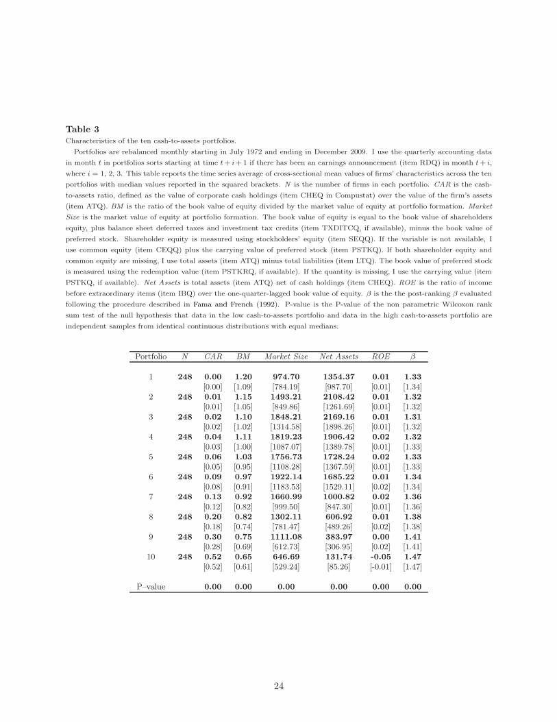
Table 3

Characteristics of the ten cash-to-assets portfolios.

.. Portfolios are rebalanced monthly starting in July 1972 and ending in December 2009. I use the quarterly accounting data

in month t in portfolios sorts starting at time t + i + 1 if there has been an earnings announcement (item RDQ) in month t + i,

where i = 1, 2, 3. This table reports the time series average of cross-sectional mean values of firms’ characteristics across the ten

portfolios with median values reported in the squared brackets. N is the number of firms in each portfolio. CAR is the cash-

to-assets ratio, defined as the value of corporate cash holdings (item CHEQ in Compustat) over the value of the firm’s assets

(item ATQ). BM is the ratio of the book value of equity divided by the market value of equity at portfolio formation. Market

Size is the market value of equity at portfolio formation. The book value of equity is equal to the book value of shareholders

equity, plus balance sheet deferred taxes and investment tax credits (item TXDITCQ, if available), minus the book value of

preferred stock. Shareholder equity is measured using stockholders’ equity (item SEQQ). If the variable is not available, I

use common equity (item CEQQ) plus the carrying value of preferred stock (item PSTKQ). If both shareholder equity and

common equity are missing, I use total assets (item ATQ) minus total liabilities (item LTQ). The book value of preferred stock

is measured using the redemption value (item PSTKRQ, if available). If the quantity is missing, I use the carrying value (item

PSTKQ, if available). Net Assets is total assets (item ATQ) net of cash holdings (item CHEQ). ROE is the ratio of income

before extraordinary items (item IBQ) over the one-quarter-lagged book value of equity. β is the the post-ranking β evaluated

following the procedure described in Fama and French (1992). P-value is the P-value of the non parametric Wilcoxon rank

sum test of the null hypothesis that data in the low cash-to-assets portfolio and data in the high cash-to-assets portfolio are

independent samples from identical continuous distributions with equal medians.

Portfolio N CAR BM Market Size Net Assets ROE β

1 248 0.00 1.20 974.70 1354.37 0.01 1.33[0.00] [1.09] [784.19] [987.70] [0.01] [1.34]

2 248 0.01 1.15 1493.21 2108.42 0.01 1.32[0.01] [1.05] [849.86] [1261.69] [0.01] [1.32]

3 248 0.02 1.10 1848.21 2169.16 0.01 1.31[0.02] [1.02] [1314.58] [1898.26] [0.01] [1.32]

4 248 0.04 1.11 1819.23 1906.42 0.02 1.32[0.03] [1.00] [1087.07] [1389.78] [0.01] [1.33]

5 248 0.06 1.03 1756.73 1728.24 0.02 1.33[0.05] [0.95] [1108.28] [1367.59] [0.01] [1.33]

6 248 0.09 0.97 1922.14 1685.22 0.01 1.34[0.08] [0.91] [1183.53] [1529.11] [0.02] [1.34]

7 248 0.13 0.92 1660.99 1000.82 0.02 1.36[0.12] [0.82] [999.50] [847.30] [0.01] [1.36]

8 248 0.20 0.82 1302.11 606.92 0.01 1.38[0.18] [0.74] [781.47] [489.26] [0.02] [1.38]

9 248 0.30 0.75 1111.08 383.97 0.00 1.41[0.28] [0.69] [612.73] [306.95] [0.02] [1.41]

10 248 0.52 0.65 646.69 131.74 -0.05 1.47[0.52] [0.61] [529.24] [85.26] [-0.01] [1.47]

P–value 0.00 0.00 0.00 0.00 0.00 0.00

24

model.10 Also, the two size measures show a hump-shaped relation with the cash-to-assets ratio.

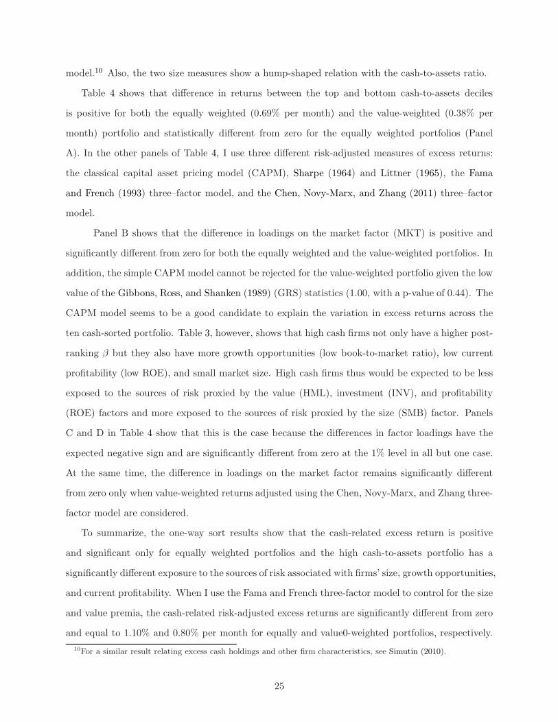
Table 4 shows that difference in returns between the top and bottom cash-to-assets deciles

is positive for both the equally weighted (0.69% per month) and the value-weighted (0.38% per

month) portfolio and statistically different from zero for the equally weighted portfolios (Panel

A). In the other panels of Table 4, I use three different risk-adjusted measures of excess returns:

the classical capital asset pricing model (CAPM), Sharpe (1964) and Littner (1965), the Fama

and French (1993) three–factor model, and the Chen, Novy-Marx, and Zhang (2011) three–factor

model.

Panel B shows that the difference in loadings on the market factor (MKT) is positive and

significantly different from zero for both the equally weighted and the value-weighted portfolios. In

addition, the simple CAPM model cannot be rejected for the value-weighted portfolio given the low

value of the Gibbons, Ross, and Shanken (1989) (GRS) statistics (1.00, with a p-value of 0.44). The

CAPM model seems to be a good candidate to explain the variation in excess returns across the

ten cash-sorted portfolio. Table 3, however, shows that high cash firms not only have a higher post-

ranking β but they also have more growth opportunities (low book-to-market ratio), low current

profitability (low ROE), and small market size. High cash firms thus would be expected to be less

exposed to the sources of risk proxied by the value (HML), investment (INV), and profitability

(ROE) factors and more exposed to the sources of risk proxied by the size (SMB) factor. Panels

C and D in Table 4 show that this is the case because the differences in factor loadings have the

expected negative sign and are significantly different from zero at the 1% level in all but one case.

At the same time, the difference in loadings on the market factor remains significantly different

from zero only when value-weighted returns adjusted using the Chen, Novy-Marx, and Zhang three-

factor model are considered.

To summarize, the one-way sort results show that the cash-related excess return is positive

and significant only for equally weighted portfolios and the high cash-to-assets portfolio has a

significantly different exposure to the sources of risk associated with firms’ size, growth opportunities,

and current profitability. When I use the Fama and French three-factor model to control for the size

and value premia, the cash-related risk-adjusted excess returns are significantly different from zero

and equal to 1.10% and 0.80% per month for equally and value0-weighted portfolios, respectively.

10For a similar result relating excess cash holdings and other firm characteristics, see Simutin (2010).

25

Table 4

Equity returns and risk-adjusted returns across the ten cash-to-assets portfolios.

.. Portfolios are rebalanced monthly starting in July 1972 and ending in December 2009. I use the quarterly accounting data in

month t in portfolios sorts starting at time t+i+1 if there has been an earnings announcement (item RDQ) in month t+i, where

i = 1, 2, 3. This table reports results for both equally weighted and value-weighted portfolios. CH1 is the bottom cash-holding

decile, CH5 is the fifth cash-holding decile, CH10 is the top cash-holding decile, and ∆CH is the difference between the top

and bottom cash-holding deciles. Panel A reports the average realized equity returns in excess of the risk-free rate and the

corresponding t-statistics. Panel B, Panel C, and Panel D report the risk-adjusted equity returns (α) and the factor loadings

(βs) with the corresponding t-statistics using the classical capital asset pricing model (Sharpe (1964), Littner (1965)), the Fama

and French (1993) three-factor model, and the Chen, Novy-Marx, and Zhang (2011) three-factor model, respectively. GRS and

p(GRS) are the Gibbons, Ross, and Shanken (1989) test statistics and the corresponding p-value, respectively. m.a.e. is the

mean absolute error of the risk-adjusted equity returns. The t-statistics are evaluated following Newey and West (1987) and

using 12 lags. The t-statistics of the difference in factor loadings between the top and bottom cash-holding deciles are evaluated

using robust t-statisctics.

Equally weighted Value-weighted

CH1 CH5 CH10 ∆CH CH1 CH5 CH10 ∆CH

Panel A: rei

= E[rit − r

ft ]

rei 0.51 0.90 1.19 0.69 0.39 0.44 0.77 0.38

tre

i1.66 2.87 2.76 2.14 1.72 1.91 2.05 1.33

Panel B: rit − r

ft = α+ βM KT (MKTt − r

ft ) + εi

t

α 0.04 0.41 0.62 0.58 -0.02 0.03 0.20 0.22

tα 0.23 2.08 2.04 1.95 -0.22 0.27 0.96 0.87

βMKT 1.08 1.15 1.34 0.26 0.96 0.97 1.34 0.38

tβMKT17.90 20.31 18.20 3.47 25.76 35.78 14.40 5.68

GRS = 4.02 p(GRS) = 0.00 m.a.e = 0.35 GRS = 1.00 p(GRS) = 0.44 m.a.e = 0.11

Panel C: rit − r

ft = α+ βM KT (MKTt − r

ft ) + βSM B SMBt + βHM LHMLt + εi

t

α -0.35 0.08 0.75 1.10 -0.12 -0.07 0.69 0.80

tα -3.21 0.72 3.08 5.47 -0.97 -0.73 3.54 3.67

βMKT 1.06 1.09 1.01 -0.05 1.01 1.01 1.08 0.07

tβMKT32.56 34.83 18.44 -0.76 30.95 38.07 16.81 1.23

βSMB 0.79 0.85 1.21 0.42 -0.03 -0.00 0.28 0.32

tβSMB7.48 8.74 11.62 3.17 -0.48 -0.06 2.64 3.27

βHML 0.55 0.43 -0.46 -1.01 0.17 0.17 -0.91 -1.09

tβHML6.49 4.91 -4.96 -9.55 2.07 2.63 -9.26 -11.67


Panel D: rit − r

ft = α + βM KT (MKTt − r

ft ) + βIN V INVt + βROEROEt + εi

t

α 0.17 0.60 1.44 1.26 -0.10 -0.03 0.80 0.89

tα 0.84 2.90 3.64 3.63 -0.87 -0.28 2.97 3.19

βMKT 1.05 1.10 1.15 0.11 0.98 0.98 1.20 0.22

tβMKT17.92 18.58 16.39 1.48 35.60 45.44 20.00 3.60

βINV 0.14 0.15 -0.19 -0.32 -0.08 -0.01 -0.58 -0.50

tβINV1.13 1.38 -1.18 -1.88 -0.91 -0.19 -3.49 -3.16

βROE -0.23 -0.32 -0.90 -0.66 0.14 0.07 -0.41 -0.55

tβROE-2.03 -3.45 -4.28 -4.05 1.91 1.02 -2.44 -4.59


26

When I use the Chen, Novy-Marx, and Zhang three-factor model to control for the investment and

profitability premia, the cash-related risk-adjusted excess returns are also significantly different

from zero and equal to 1.26% and 0.89% per month for equally and value weighted portfolios,

respectively.

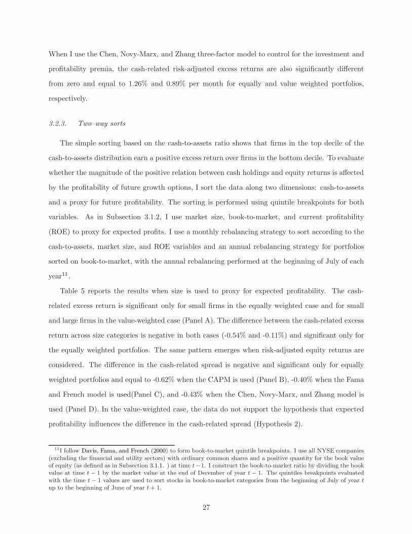
3.2.3. Two–way sorts

The simple sorting based on the cash-to-assets ratio shows that firms in the top decile of the

cash-to-assets distribution earn a positive excess return over firms in the bottom decile. To evaluate

whether the magnitude of the positive relation between cash holdings and equity returns is affected

by the profitability of future growth options, I sort the data along two dimensions: cash-to-assets

and a proxy for future profitability. The sorting is performed using quintile breakpoints for both

variables. As in Subsection 3.1.2, I use market size, book-to-market, and current profitability

(ROE) to proxy for expected profits. I use a monthly rebalancing strategy to sort according to the

cash-to-assets, market size, and ROE variables and an annual rebalancing strategy for portfolios

sorted on book-to-market, with the annual rebalancing performed at the beginning of July of each

year11.

Table 5 reports the results when size is used to proxy for expected profitability. The cash-

related excess return is significant only for small firms in the equally weighted case and for small

and large firms in the value-weighted case (Panel A). The difference between the cash-related excess

return across size categories is negative in both cases (-0.54% and -0.11%) and significant only for

the equally weighted portfolios. The same pattern emerges when risk-adjusted equity returns are

considered. The difference in the cash-related spread is negative and significant only for equally

weighted portfolios and equal to -0.62% when the CAPM is used (Panel B), -0.40% when the Fama

and French model is used(Panel C), and -0.43% when the Chen, Novy-Marx, and Zhang model is

used (Panel D). In the value-weighted case, the data do not support the hypothesis that expected

profitability influences the difference in the cash-related spread (Hypothesis 2).

11I follow Davis, Fama, and French (2000) to form book-to-market quintile breakpoints. I use all NYSE companies(excluding the financial and utility sectors) with ordinary common shares and a positive quantity for the book valueof equity (as defined as in Subsection 3.1.1. ) at time t−1. I construct the book-to-market ratio by dividing the bookvalue at time t − 1 by the market value at the end of December of year t − 1. The quintiles breakpoints evaluatedwith the time t − 1 values are used to sort stocks in book-to-market categories from the beginning of July of year tup to the beginning of June of year t + 1.

27

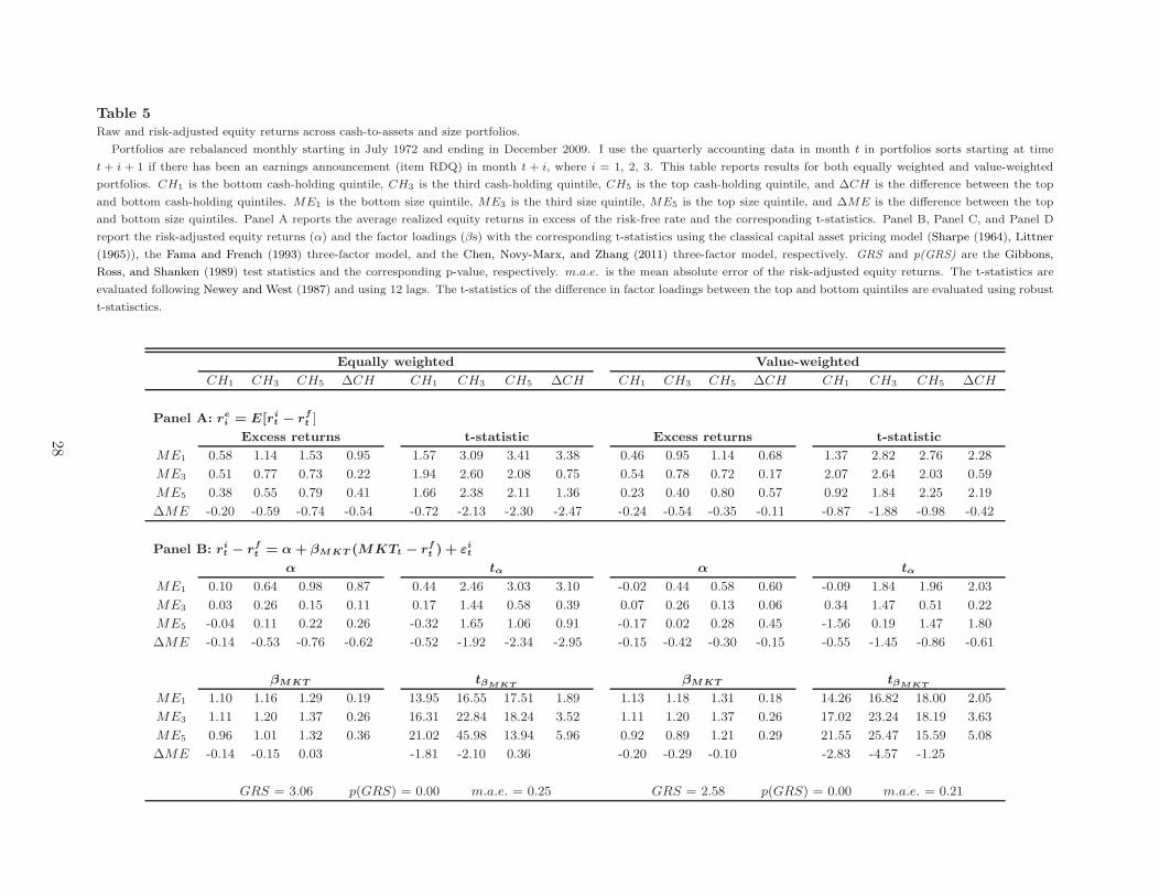
Table 5

Raw and risk-adjusted equity returns across cash-to-assets and size portfolios.

.. Portfolios are rebalanced monthly starting in July 1972 and ending in December 2009. I use the quarterly accounting data in month t in portfolios sorts starting at time

t + i + 1 if there has been an earnings announcement (item RDQ) in month t + i, where i = 1, 2, 3. This table reports results for both equally weighted and value-weighted

portfolios. CH1 is the bottom cash-holding quintile, CH3 is the third cash-holding quintile, CH5 is the top cash-holding quintile, and ∆CH is the difference between the top

and bottom cash-holding quintiles. ME1 is the bottom size quintile, ME3 is the third size quintile, ME5 is the top size quintile, and ∆ME is the difference between the top

and bottom size quintiles. Panel A reports the average realized equity returns in excess of the risk-free rate and the corresponding t-statistics. Panel B, Panel C, and Panel D

report the risk-adjusted equity returns (α) and the factor loadings (βs) with the corresponding t-statistics using the classical capital asset pricing model (Sharpe (1964), Littner

(1965)), the Fama and French (1993) three-factor model, and the Chen, Novy-Marx, and Zhang (2011) three-factor model, respectively. GRS and p(GRS) are the Gibbons,

Ross, and Shanken (1989) test statistics and the corresponding p-value, respectively. m.a.e. is the mean absolute error of the risk-adjusted equity returns. The t-statistics are

evaluated following Newey and West (1987) and using 12 lags. The t-statistics of the difference in factor loadings between the top and bottom quintiles are evaluated using robust

t-statisctics.


CH1 CH3 CH5 ∆CH CH1 CH3 CH5 ∆CH CH1 CH3 CH5 ∆CH CH1 CH3 CH5 ∆CH

Panel A: rei = E[ri

t − rft ]

Excess returns t-statistic Excess returns t-statistic

ME1 0.58 1.14 1.53 0.95 1.57 3.09 3.41 3.38 0.46 0.95 1.14 0.68 1.37 2.82 2.76 2.28

ME3 0.51 0.77 0.73 0.22 1.94 2.60 2.08 0.75 0.54 0.78 0.72 0.17 2.07 2.64 2.03 0.59

ME5 0.38 0.55 0.79 0.41 1.66 2.38 2.11 1.36 0.23 0.40 0.80 0.57 0.92 1.84 2.25 2.19

∆ME -0.20 -0.59 -0.74 -0.54 -0.72 -2.13 -2.30 -2.47 -0.24 -0.54 -0.35 -0.11 -0.87 -1.88 -0.98 -0.42

Panel B: rit − r


ft ) + εi

t

α tα α tα

ME1 0.10 0.64 0.98 0.87 0.44 2.46 3.03 3.10 -0.02 0.44 0.58 0.60 -0.09 1.84 1.96 2.03

ME3 0.03 0.26 0.15 0.11 0.17 1.44 0.58 0.39 0.07 0.26 0.13 0.06 0.34 1.47 0.51 0.22

ME5 -0.04 0.11 0.22 0.26 -0.32 1.65 1.06 0.91 -0.17 0.02 0.28 0.45 -1.56 0.19 1.47 1.80

∆ME -0.14 -0.53 -0.76 -0.62 -0.52 -1.92 -2.34 -2.95 -0.15 -0.42 -0.30 -0.15 -0.55 -1.45 -0.86 -0.61

βM KT tβMKTβM KT tβMKT

ME1 1.10 1.16 1.29 0.19 13.95 16.55 17.51 1.89 1.13 1.18 1.31 0.18 14.26 16.82 18.00 2.05

ME3 1.11 1.20 1.37 0.26 16.31 22.84 18.24 3.52 1.11 1.20 1.37 0.26 17.02 23.24 18.19 3.63

ME5 0.96 1.01 1.32 0.36 21.02 45.98 13.94 5.96 0.92 0.89 1.21 0.29 21.55 25.47 15.59 5.08

∆ME -0.14 -0.15 0.03 -1.81 -2.10 0.36 -0.20 -0.29 -0.10 -2.83 -4.57 -1.25

GRS = 3.06 p(GRS) = 0.00 m.a.e. = 0.25 GRS = 2.58 p(GRS) = 0.00 m.a.e. = 0.21

28

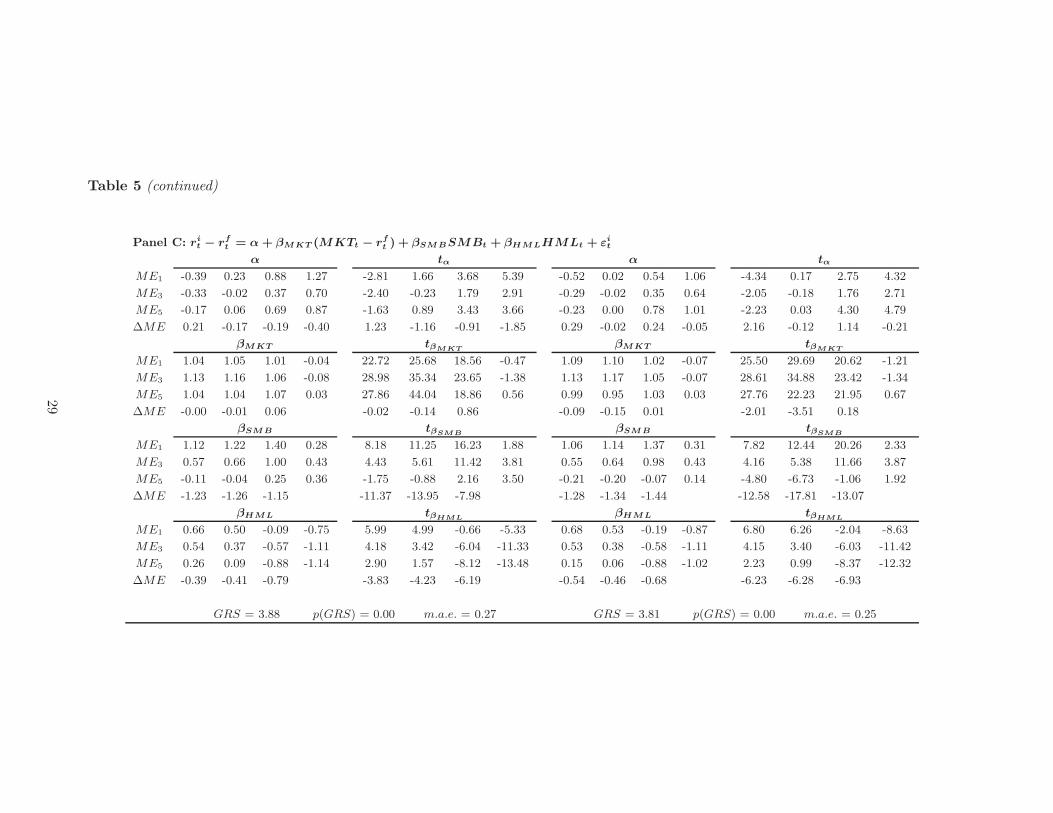
Table 5 (continued)

Panel C: rit − r


ft ) + βSM BSMBt + βHM LHMLt + εi

t

α tα α tα

ME1 -0.39 0.23 0.88 1.27 -2.81 1.66 3.68 5.39 -0.52 0.02 0.54 1.06 -4.34 0.17 2.75 4.32

ME3 -0.33 -0.02 0.37 0.70 -2.40 -0.23 1.79 2.91 -0.29 -0.02 0.35 0.64 -2.05 -0.18 1.76 2.71

ME5 -0.17 0.06 0.69 0.87 -1.63 0.89 3.43 3.66 -0.23 0.00 0.78 1.01 -2.23 0.03 4.30 4.79

∆ME 0.21 -0.17 -0.19 -0.40 1.23 -1.16 -0.91 -1.85 0.29 -0.02 0.24 -0.05 2.16 -0.12 1.14 -0.21


ME1 1.04 1.05 1.01 -0.04 22.72 25.68 18.56 -0.47 1.09 1.10 1.02 -0.07 25.50 29.69 20.62 -1.21

ME3 1.13 1.16 1.06 -0.08 28.98 35.34 23.65 -1.38 1.13 1.17 1.05 -0.07 28.61 34.88 23.42 -1.34

ME5 1.04 1.04 1.07 0.03 27.86 44.04 18.86 0.56 0.99 0.95 1.03 0.03 27.76 22.23 21.95 0.67

∆ME -0.00 -0.01 0.06 -0.02 -0.14 0.86 -0.09 -0.15 0.01 -2.01 -3.51 0.18

βSM B tβSMBβSM B tβSMB

ME1 1.12 1.22 1.40 0.28 8.18 11.25 16.23 1.88 1.06 1.14 1.37 0.31 7.82 12.44 20.26 2.33

ME3 0.57 0.66 1.00 0.43 4.43 5.61 11.42 3.81 0.55 0.64 0.98 0.43 4.16 5.38 11.66 3.87

ME5 -0.11 -0.04 0.25 0.36 -1.75 -0.88 2.16 3.50 -0.21 -0.20 -0.07 0.14 -4.80 -6.73 -1.06 1.92

∆ME -1.23 -1.26 -1.15 -11.37 -13.95 -7.98 -1.28 -1.34 -1.44 -12.58 -17.81 -13.07

βHM L tβHMLβHM L tβHML

ME1 0.66 0.50 -0.09 -0.75 5.99 4.99 -0.66 -5.33 0.68 0.53 -0.19 -0.87 6.80 6.26 -2.04 -8.63

ME3 0.54 0.37 -0.57 -1.11 4.18 3.42 -6.04 -11.33 0.53 0.38 -0.58 -1.11 4.15 3.40 -6.03 -11.42

ME5 0.26 0.09 -0.88 -1.14 2.90 1.57 -8.12 -13.48 0.15 0.06 -0.88 -1.02 2.23 0.99 -8.37 -12.32

∆ME -0.39 -0.41 -0.79 -3.83 -4.23 -6.19 -0.54 -0.46 -0.68 -6.23 -6.28 -6.93


29

Table 5 (continued)

Panel D: rit − r



t

α tα α tα

ME1 0.39 1.03 1.85 1.46 1.46 3.74 4.71 5.58 0.10 0.68 1.33 1.23 0.42 2.77 3.43 4.39

ME3 -0.00 0.27 0.70 0.71 -0.02 1.61 1.84 2.63 0.03 0.26 0.68 0.65 0.16 1.53 1.81 2.46

ME5 -0.23 0.09 0.80 1.03 -2.20 1.17 2.63 4.28 -0.38 -0.10 0.69 1.08 -3.36 -0.99 2.69 4.77

∆ME -0.62 -0.94 -1.04 -0.43 -2.55 -3.48 -3.33 -2.06 -0.49 -0.78 -0.64 -0.16 -1.85 -2.67 -1.81 -0.60


ME1 1.04 1.07 1.09 0.05 13.13 13.14 13.12 0.59 1.10 1.13 1.14 0.04 14.22 15.24 15.14 0.50

ME3 1.12 1.19 1.25 0.12 20.20 24.66 20.74 1.73 1.11 1.20 1.24 0.13 21.20 25.60 20.96 1.81

ME5 1.01 1.02 1.18 0.18 42.43 67.97 20.26 3.43 0.97 0.92 1.12 0.15 37.16 37.13 20.85 2.76

∆ME -0.03 -0.05 0.09 -0.43 -0.79 1.21 -0.13 -0.21 -0.02 -1.88 -3.51 -0.32

βIN V tβINVβIN V tβINV

ME1 0.22 0.23 -0.05 -0.27 1.26 1.43 -0.26 -1.20 0.28 0.29 0.00 -0.28 1.86 2.25 0.00 -1.42

ME3 -0.02 0.11 -0.20 -0.18 -0.17 1.28 -1.12 -0.97 -0.02 0.12 -0.21 -0.19 -0.23 1.35 -1.21 -1.01

ME5 0.02 -0.06 -0.56 -0.58 0.22 -1.06 -3.29 -4.11 0.07 -0.00 -0.54 -0.61 0.97 -0.03 -3.22 -4.21

∆ME -0.20 -0.29 -0.51 -1.27 -1.91 -2.43 -0.20 -0.29 -0.54 -1.40 -2.24 -2.74

βROE tβROEβROE tβROE

ME1 -0.47 -0.61 -1.04 -0.57 -3.32 -5.60 -6.42 -3.36 -0.31 -0.46 -0.92 -0.62 -2.28 -4.66 -5.13 -3.96

ME3 0.06 -0.07 -0.57 -0.63 0.37 -0.78 -2.51 -3.86 0.06 -0.06 -0.56 -0.62 0.40 -0.60 -2.47 -3.89

ME5 0.23 0.06 -0.40 -0.63 2.58 0.84 -2.00 -5.05 0.22 0.14 -0.21 -0.43 3.97 2.86 -1.50 -4.49

∆ME 0.70 0.67 0.64 6.04 6.64 3.65 0.52 0.60 0.71 4.99 6.80 4.77


30

Table 5 also reports the loading on each risk factor used to risk-adjust the excess returns. Similar

to the one-way sort case, the significance of the difference in loadings on the market factor weakens

substantially when the Fama and French or the Chen, Novy-Marx, and Zhang factor model is used,

at the same time, high cash portfolios are significantly less exposed to the sources of risk proxied

by the HML and the ROE factors. Panel C shows that the difference in loadings on the HML

factor varies between -1.14 (large size portfolio) and -0.75 (small size portfolio), thus generating a

substantial spread of -0.19% per month in the cash-related excess return between large and small

firms12. Panel D shows that, for the large firms category, high cash firms are less exposed to the

investment factor and this is expected given that the investment factor has properties similar to

the HML factor, as Chen, Novy-Marx, and Zhang (2011) show. In addition, high cash firms have a

significant smaller loading on the ROE factor that varies between -0.63 and -0.57 (-0.62 and -0.43)

in the equally (value-) weighted case. These results confirm what is found in the one-way sort case.

The cash-related risk-adjusted excess returns increase after the sources of risk associated to firms’

size, growth opportunities and current profitability are controlled for.

Table 6 and Table 7 report the outcome of the two-way sorts on cash-to-assets and book-to-

market and cash-to-assets and return on equity, respectively. The results are very similar to the

ones described for the cash-to-assets and size-sorted portfolios. When the book-to-market ratio is

used to proxy for expected profitability, more support is found for the hypothesis that expected

profitability influences the difference in the cash-related spread because the spread is now positive

and significant for both equally weighted (1.28% per month) and value-weighted (0.75% per month)

portfolios. Panel C and Panel D of Table 6 show that the high cash portfolios are significantly less

exposed to the value and the profitability risk factors, but they still earn a significantly larger excess

return than low cash portfolios.

Using a third proxy for expected profitability, I get a significantly larger cash-related spread

(0.87% per month) only for low ROE portfolios in the equally weighted case (Table 7, Panel A).

As in the previous two cases and in the one-sort case, high cash firms have larger factor loadings

on the value and profitability factors (Table 7, Panel C and Panel D). It is worth highlighting that

12The average value of the HML factor over the period that starts in July 1972 and ends in December 2009 is equalto 0.47%. The different exposure to the value factor generates a difference in returns between high cash and low cashfirms equal to -0.75×0.47 = -0.35% (-1.14×0.47 = -0.54%) for small (large) size firms. The implied difference in thecash-related spread between large (more profitable) and small (less profitable) firms is equal to -0.54% - (-0.35)% =-0.19%.

31

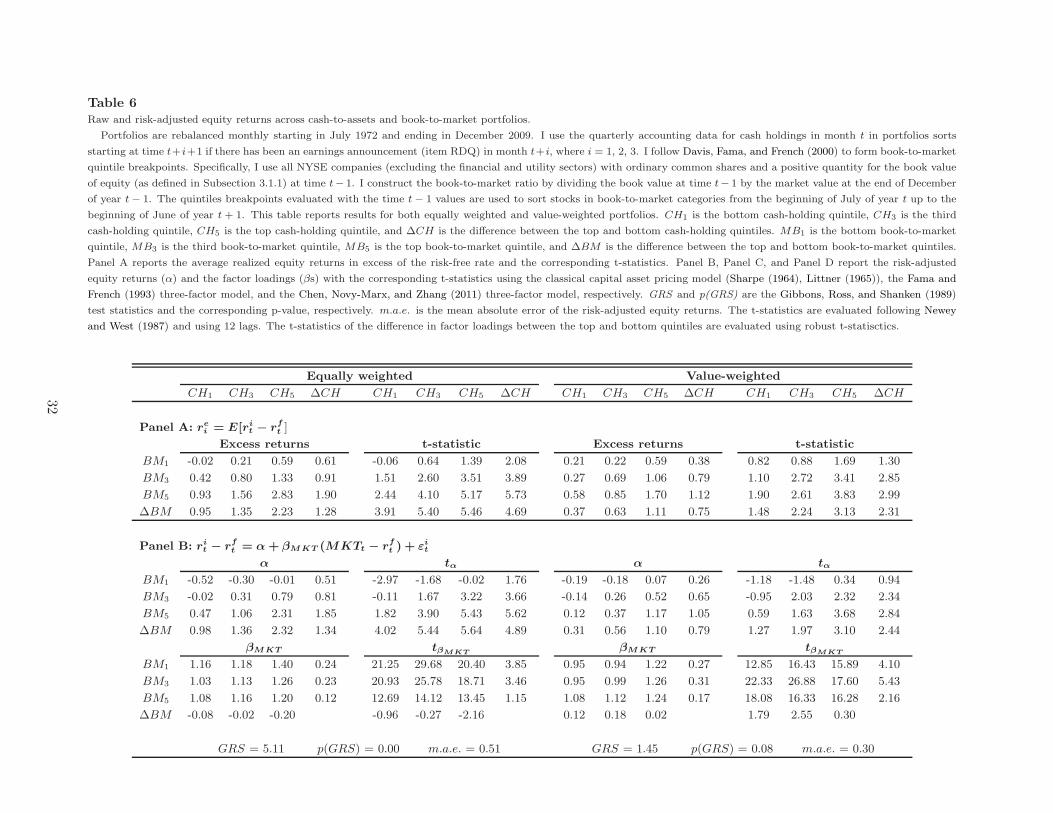
Table 6

Raw and risk-adjusted equity returns across cash-to-assets and book-to-market portfolios.

.. Portfolios are rebalanced monthly starting in July 1972 and ending in December 2009. I use the quarterly accounting data for cash holdings in month t in portfolios sorts

starting at time t+i+1 if there has been an earnings announcement (item RDQ) in month t+i, where i = 1, 2, 3. I follow Davis, Fama, and French (2000) to form book-to-market

quintile breakpoints. Specifically, I use all NYSE companies (excluding the financial and utility sectors) with ordinary common shares and a positive quantity for the book value

of equity (as defined in Subsection 3.1.1) at time t− 1. I construct the book-to-market ratio by dividing the book value at time t− 1 by the market value at the end of December

of year t − 1. The quintiles breakpoints evaluated with the time t − 1 values are used to sort stocks in book-to-market categories from the beginning of July of year t up to the

beginning of June of year t + 1. This table reports results for both equally weighted and value-weighted portfolios. CH1 is the bottom cash-holding quintile, CH3 is the third

cash-holding quintile, CH5 is the top cash-holding quintile, and ∆CH is the difference between the top and bottom cash-holding quintiles. MB1 is the bottom book-to-market

quintile, MB3 is the third book-to-market quintile, MB5 is the top book-to-market quintile, and ∆BM is the difference between the top and bottom book-to-market quintiles.

Panel A reports the average realized equity returns in excess of the risk-free rate and the corresponding t-statistics. Panel B, Panel C, and Panel D report the risk-adjusted

equity returns (α) and the factor loadings (βs) with the corresponding t-statistics using the classical capital asset pricing model (Sharpe (1964), Littner (1965)), the Fama and

French (1993) three-factor model, and the Chen, Novy-Marx, and Zhang (2011) three-factor model, respectively. GRS and p(GRS) are the Gibbons, Ross, and Shanken (1989)

test statistics and the corresponding p-value, respectively. m.a.e. is the mean absolute error of the risk-adjusted equity returns. The t-statistics are evaluated following Newey

and West (1987) and using 12 lags. The t-statistics of the difference in factor loadings between the top and bottom quintiles are evaluated using robust t-statisctics.


CH1 CH3 CH5 ∆CH CH1 CH3 CH5 ∆CH CH1 CH3 CH5 ∆CH CH1 CH3 CH5 ∆CH

Panel A: rei = E[ri

t − rft ]

Excess returns t-statistic Excess returns t-statistic

BM1 -0.02 0.21 0.59 0.61 -0.06 0.64 1.39 2.08 0.21 0.22 0.59 0.38 0.82 0.88 1.69 1.30

BM3 0.42 0.80 1.33 0.91 1.51 2.60 3.51 3.89 0.27 0.69 1.06 0.79 1.10 2.72 3.41 2.85

BM5 0.93 1.56 2.83 1.90 2.44 4.10 5.17 5.73 0.58 0.85 1.70 1.12 1.90 2.61 3.83 2.99

∆BM 0.95 1.35 2.23 1.28 3.91 5.40 5.46 4.69 0.37 0.63 1.11 0.75 1.48 2.24 3.13 2.31

Panel B: rit − r


ft ) + εi

t

α tα α tα

BM1 -0.52 -0.30 -0.01 0.51 -2.97 -1.68 -0.02 1.76 -0.19 -0.18 0.07 0.26 -1.18 -1.48 0.34 0.94

BM3 -0.02 0.31 0.79 0.81 -0.11 1.67 3.22 3.66 -0.14 0.26 0.52 0.65 -0.95 2.03 2.32 2.34

BM5 0.47 1.06 2.31 1.85 1.82 3.90 5.43 5.62 0.12 0.37 1.17 1.05 0.59 1.63 3.68 2.84

∆BM 0.98 1.36 2.32 1.34 4.02 5.44 5.64 4.89 0.31 0.56 1.10 0.79 1.27 1.97 3.10 2.44


BM1 1.16 1.18 1.40 0.24 21.25 29.68 20.40 3.85 0.95 0.94 1.22 0.27 12.85 16.43 15.89 4.10

BM3 1.03 1.13 1.26 0.23 20.93 25.78 18.71 3.46 0.95 0.99 1.26 0.31 22.33 26.88 17.60 5.43

BM5 1.08 1.16 1.20 0.12 12.69 14.12 13.45 1.15 1.08 1.12 1.24 0.17 18.08 16.33 16.28 2.16

∆BM -0.08 -0.02 -0.20 -0.96 -0.27 -2.16 0.12 0.18 0.02 1.79 2.55 0.30


32

Table 6 (continued)

Panel C: rit − r



t

α tα α tα

BM1 -0.63 -0.30 0.28 0.92 -3.88 -2.47 1.21 3.59 -0.16 -0.03 0.57 0.73 -0.93 -0.22 3.04 2.90

BM3 -0.32 0.05 0.74 1.06 -2.24 0.53 4.34 4.99 -0.33 0.09 0.61 0.94 -2.20 0.72 3.09 3.80

BM5 -0.07 0.54 2.03 2.10 -0.42 3.12 5.35 6.81 -0.24 -0.09 0.99 1.23 -1.23 -0.38 3.46 3.57

∆BM 0.56 0.84 1.74 1.18 2.78 4.18 4.76 4.35 -0.07 -0.06 0.42 0.49 -0.32 -0.25 1.45 1.62


BM1 1.05 1.04 1.07 0.02 24.90 36.14 21.73 0.39 0.97 0.92 1.00 0.03 15.18 19.96 22.67 0.59

BM3 0.99 1.07 1.04 0.04 20.46 32.51 20.54 0.81 1.02 1.06 1.09 0.07 24.08 21.82 18.21 1.23

BM5 1.09 1.13 1.05 -0.03 21.76 22.95 12.20 -0.33 1.16 1.23 1.14 -0.02 25.44 12.91 16.40 -0.28

∆BM 0.04 0.09 -0.02 0.58 1.53 -0.20 0.19 0.31 0.14 3.05 4.40 2.00


BM1 0.68 0.63 0.93 0.25 9.62 9.82 7.57 2.16 -0.13 -0.18 0.07 0.20 -2.28 -3.44 1.02 2.47

BM3 0.69 0.75 1.06 0.38 5.99 10.56 14.42 3.55 0.03 0.02 0.59 0.56 0.41 0.23 6.58 6.00

BM5 0.93 1.04 1.16 0.24 7.91 7.63 7.85 1.40 0.25 0.34 0.77 0.52 2.38 2.76 7.57 3.90

∆BM 0.25 0.41 0.24 2.33 3.40 1.37 0.38 0.52 0.71 3.67 4.96 6.03


BM1 0.08 -0.11 -0.69 -0.77 0.95 -1.24 -7.73 -8.30 -0.03 -0.25 -0.90 -0.87 -0.26 -2.27 -9.22 -8.94

BM3 0.40 0.32 -0.12 -0.52 3.41 4.27 -1.42 -5.53 0.34 0.29 -0.27 -0.61 3.65 3.53 -3.49 -6.20

BM5 0.78 0.72 0.29 -0.49 7.25 5.85 1.45 -2.67 0.58 0.74 0.17 -0.40 5.53 4.83 1.28 -2.98

∆BM 0.70 0.83 0.98 6.18 7.06 5.73 0.61 0.99 1.07 5.58 8.22 8.51


33

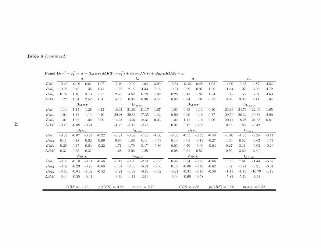
Table 6 (continued)

Panel D: rit − r



t

α tα α tα

BM1 -0.46 -0.18 0.61 1.07 -2.40 -0.99 1.64 3.99 -0.54 -0.42 0.48 1.02 -4.00 -3.38 1.82 4.54

BM3 -0.05 0.42 1.35 1.41 -0.27 2.14 4.33 7.16 -0.31 0.29 0.97 1.28 -1.84 1.97 3.06 4.72

BM5 0.76 1.46 3.13 2.37 2.55 4.62 6.78 7.92 0.28 0.43 1.82 1.54 1.06 1.58 5.81 4.63

∆BM 1.22 1.64 2.52 1.30 5.15 6.85 6.36 4.72 0.82 0.84 1.34 0.52 3.84 3.33 4.14 1.64


BM1 1.14 1.15 1.26 0.12 18.31 21.66 21.17 1.67 1.03 0.99 1.13 0.10 23.83 24.76 22.09 1.65

BM3 1.04 1.11 1.14 0.10 20.08 20.86 17.35 1.42 0.99 0.99 1.16 0.17 29.50 26.32 19.81 2.90

BM5 1.01 1.07 1.02 0.00 14.38 14.02 12.31 0.03 1.04 1.11 1.10 0.06 20.14 18.28 21.63 0.81

∆BM -0.13 -0.08 -0.24 -1.72 -1.15 -2.76 0.01 0.12 -0.03 0.15 1.83 -0.42


BM1 -0.05 -0.07 -0.27 -0.22 -0.31 -0.68 -1.86 -1.30 -0.05 -0.11 -0.53 -0.48 -0.40 -1.35 -3.25 -3.11

BM3 0.11 0.18 0.02 -0.09 0.86 1.86 0.11 -0.53 0.14 0.05 -0.13 -0.27 1.39 0.52 -0.63 -1.57

BM5 0.26 0.27 0.04 -0.22 1.71 1.79 0.17 -0.86 0.03 0.50 -0.00 -0.04 0.27 3.11 -0.03 -0.20

∆BM 0.31 0.35 0.31 1.68 2.06 1.25 0.08 0.61 0.52 0.56 3.60 2.60


BM1 -0.05 -0.10 -0.61 -0.56 -0.47 -0.90 -2.51 -3.55 0.45 0.34 -0.22 -0.66 11.53 7.61 -1.44 -6.67

BM3 -0.02 -0.23 -0.70 -0.68 -0.31 -3.55 -6.91 -6.66 0.14 -0.06 -0.48 -0.62 1.47 -0.71 -5.21 -6.31

BM5 -0.50 -0.64 -1.02 -0.52 -3.24 -4.68 -9.78 -3.02 -0.21 -0.34 -0.79 -0.58 -1.41 -1.73 -10.79 -4.18

∆BM -0.46 -0.55 -0.41 -3.49 -4.11 -2.14 -0.66 -0.69 -0.58 -5.82 -5.79 -4.54


34

Table 7

Raw and risk-adjusted equity returns across cash-to-assets and return on equity (ROE) portfolios.

.. Portfolios are rebalanced monthly starting in July 1972 and ending in December 2009. I use the quarterly accounting data in month t in portfolios sorts starting at time

t + i + 1 if there has been an earnings announcement (item RDQ) in month t + i, where i = 1, 2, 3. This table reports results for both equally weighted and value-weighted

portfolios. CH1 is the bottom cash-holding quintile, CH3 is the third cash-holding quintile, CH5 is the top cash-holding quintile, and ∆CH is the difference between the top and

bottom cash-holding quintiles. ROE1 is the bottom ROE quintile, ROE3 is the third ROE quintile, ROE5 is the top ROE quintile, and ∆ROE is the difference between the top

and bottom ROE quintiles. Panel A reports the average realized equity returns in excess of the risk-free rate and the corresponding t-statistics. Panel B, Panel C, and Panel D

report the risk-adjusted equity returns (α) and the factor loadings (βs) with the corresponding t-statistics using the classical capital asset pricing model (Sharpe (1964), Littner

(1965)), the Fama and French (1993) three-factor model, and the Chen, Novy-Marx, and Zhang (2011) three-factor model, respectively. GRS and p(GRS) are the Gibbons,

Ross, and Shanken (1989) test statistics and the corresponding p-value, respectively. m.a.e. is the mean absolute error of the risk-adjusted equity returns. The t-statistics are

evaluated following Newey and West (1987) and using 12 lags. The t-statistics of the difference in factor loadings between the top and bottom quintiles are evaluated using robust

t-statisctics.

Equally weighted Value-weightedCH1 CH3 CH5 ∆CH CH1 CH3 CH5 ∆CH CH1 CH3 CH5 ∆CH CH1 CH3 CH5 ∆CH

Panel A: rei = E[ri

t − rft ]

Excess returns t-statistic Excess returns t-statisticROE1 -0.32 0.62 1.04 1.36 -0.68 1.33 2.02 4.10 -0.66 0.14 0.17 0.83 -1.40 0.29 0.40 2.05ROE3 0.70 0.94 1.01 0.31 2.49 3.32 3.11 1.26 0.43 0.29 0.69 0.27 1.94 1.17 1.82 0.86ROE5 0.93 1.28 1.44 0.51 2.90 4.13 4.13 2.09 0.45 0.64 0.88 0.43 1.53 2.54 2.50 1.40∆ROE 1.25 0.66 0.40 -0.85 3.85 1.96 1.47 -3.17 1.11 0.50 0.71 -0.40 2.92 1.23 2.65 -1.06

Panel B: rit − r


ft ) + εi

t

α tα α tα

ROE1 -0.86 0.03 0.42 1.28 -2.80 0.09 1.09 3.79 -1.23 -0.46 -0.42 0.80 -3.77 -1.49 -1.51 1.97ROE3 0.25 0.48 0.49 0.25 1.33 2.46 2.40 1.02 0.02 -0.15 0.12 0.10 0.19 -1.16 0.51 0.34ROE5 0.44 0.79 0.88 0.44 2.24 4.38 4.44 1.79 0.02 0.24 0.35 0.33 0.12 1.77 1.86 1.10∆ROE 1.30 0.76 0.46 -0.85 4.10 2.27 1.69 -3.15 1.25 0.70 0.78 -0.47 3.42 1.84 2.91 -1.26


ROE1 1.25 1.37 1.44 0.19 14.36 15.51 15.03 1.51 1.31 1.40 1.38 0.07 19.58 14.59 13.64 0.76ROE3 1.05 1.08 1.19 0.14 16.95 20.25 19.73 2.20 0.95 1.01 1.34 0.39 23.13 31.61 11.28 4.73ROE5 1.13 1.14 1.31 0.18 18.25 18.58 23.28 2.89 0.99 0.93 1.23 0.23 14.20 15.69 19.07 3.76∆ROE -0.12 -0.23 -0.13 -1.25 -2.57 -1.38 -0.32 -0.46 -0.16 -4.44 -5.85 -1.84


35

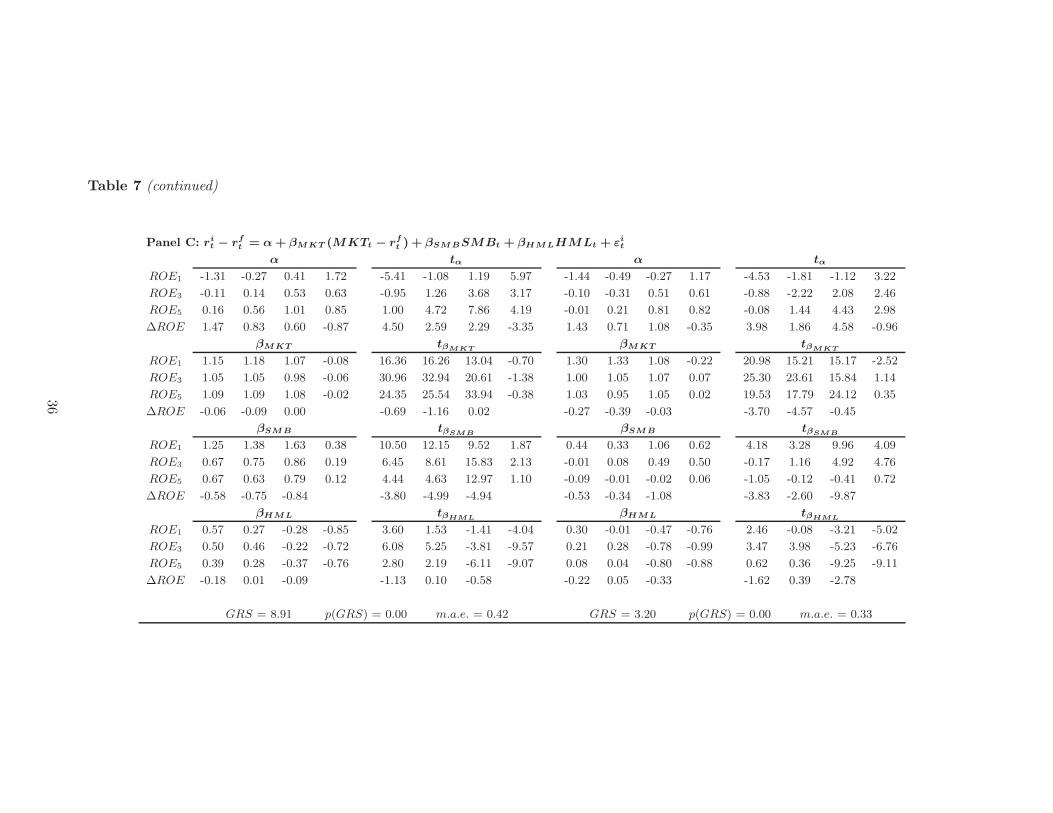
Table 7 (continued)

Panel C: rit − r



t

α tα α tα

ROE1 -1.31 -0.27 0.41 1.72 -5.41 -1.08 1.19 5.97 -1.44 -0.49 -0.27 1.17 -4.53 -1.81 -1.12 3.22

ROE3 -0.11 0.14 0.53 0.63 -0.95 1.26 3.68 3.17 -0.10 -0.31 0.51 0.61 -0.88 -2.22 2.08 2.46

ROE5 0.16 0.56 1.01 0.85 1.00 4.72 7.86 4.19 -0.01 0.21 0.81 0.82 -0.08 1.44 4.43 2.98

∆ROE 1.47 0.83 0.60 -0.87 4.50 2.59 2.29 -3.35 1.43 0.71 1.08 -0.35 3.98 1.86 4.58 -0.96


ROE1 1.15 1.18 1.07 -0.08 16.36 16.26 13.04 -0.70 1.30 1.33 1.08 -0.22 20.98 15.21 15.17 -2.52

ROE3 1.05 1.05 0.98 -0.06 30.96 32.94 20.61 -1.38 1.00 1.05 1.07 0.07 25.30 23.61 15.84 1.14

ROE5 1.09 1.09 1.08 -0.02 24.35 25.54 33.94 -0.38 1.03 0.95 1.05 0.02 19.53 17.79 24.12 0.35

∆ROE -0.06 -0.09 0.00 -0.69 -1.16 0.02 -0.27 -0.39 -0.03 -3.70 -4.57 -0.45


ROE1 1.25 1.38 1.63 0.38 10.50 12.15 9.52 1.87 0.44 0.33 1.06 0.62 4.18 3.28 9.96 4.09

ROE3 0.67 0.75 0.86 0.19 6.45 8.61 15.83 2.13 -0.01 0.08 0.49 0.50 -0.17 1.16 4.92 4.76

ROE5 0.67 0.63 0.79 0.12 4.44 4.63 12.97 1.10 -0.09 -0.01 -0.02 0.06 -1.05 -0.12 -0.41 0.72

∆ROE -0.58 -0.75 -0.84 -3.80 -4.99 -4.94 -0.53 -0.34 -1.08 -3.83 -2.60 -9.87


ROE1 0.57 0.27 -0.28 -0.85 3.60 1.53 -1.41 -4.04 0.30 -0.01 -0.47 -0.76 2.46 -0.08 -3.21 -5.02

ROE3 0.50 0.46 -0.22 -0.72 6.08 5.25 -3.81 -9.57 0.21 0.28 -0.78 -0.99 3.47 3.98 -5.23 -6.76

ROE5 0.39 0.28 -0.37 -0.76 2.80 2.19 -6.11 -9.07 0.08 0.04 -0.80 -0.88 0.62 0.36 -9.25 -9.11

∆ROE -0.18 0.01 -0.09 -1.13 0.10 -0.58 -0.22 0.05 -0.33 -1.62 0.39 -2.78


36

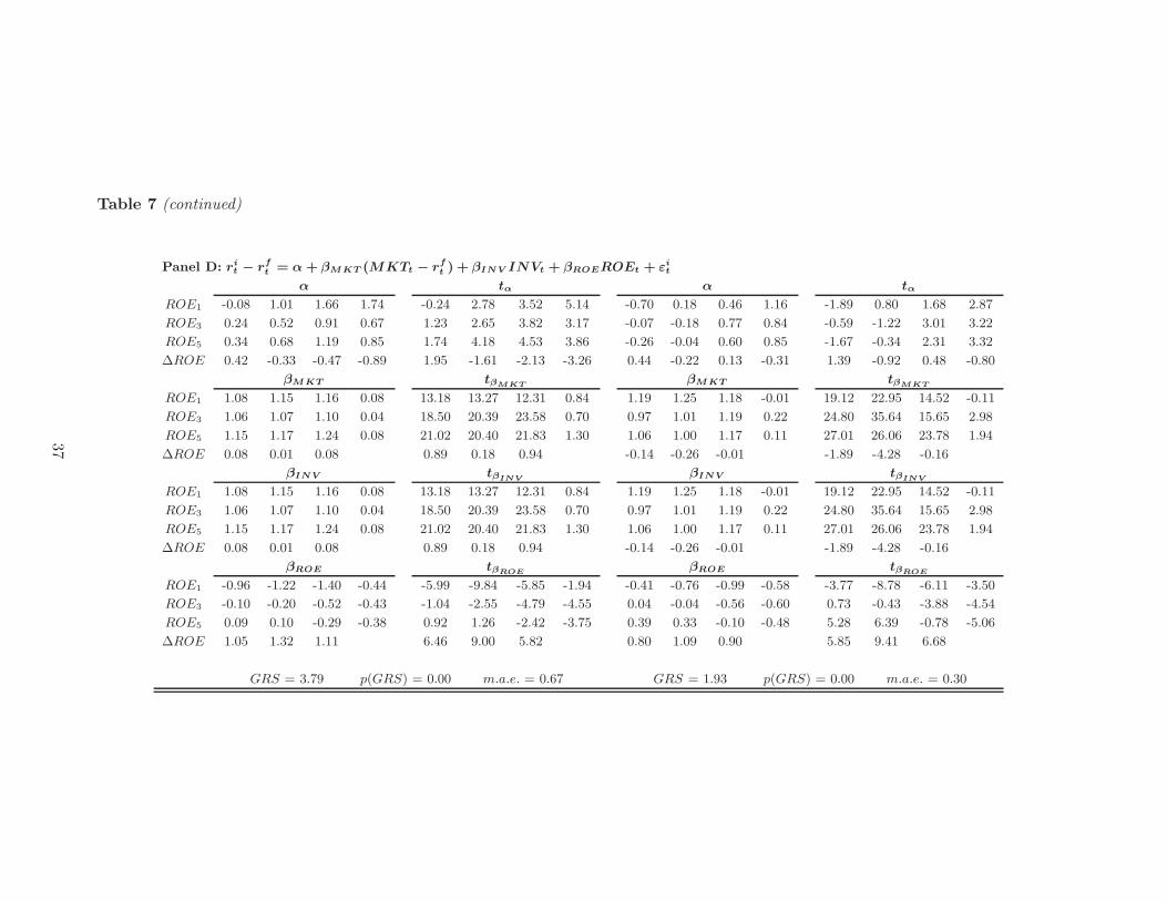
Table 7 (continued)

Panel D: rit − r



t

α tα α tα

ROE1 -0.08 1.01 1.66 1.74 -0.24 2.78 3.52 5.14 -0.70 0.18 0.46 1.16 -1.89 0.80 1.68 2.87

ROE3 0.24 0.52 0.91 0.67 1.23 2.65 3.82 3.17 -0.07 -0.18 0.77 0.84 -0.59 -1.22 3.01 3.22

ROE5 0.34 0.68 1.19 0.85 1.74 4.18 4.53 3.86 -0.26 -0.04 0.60 0.85 -1.67 -0.34 2.31 3.32

∆ROE 0.42 -0.33 -0.47 -0.89 1.95 -1.61 -2.13 -3.26 0.44 -0.22 0.13 -0.31 1.39 -0.92 0.48 -0.80


ROE1 1.08 1.15 1.16 0.08 13.18 13.27 12.31 0.84 1.19 1.25 1.18 -0.01 19.12 22.95 14.52 -0.11

ROE3 1.06 1.07 1.10 0.04 18.50 20.39 23.58 0.70 0.97 1.01 1.19 0.22 24.80 35.64 15.65 2.98

ROE5 1.15 1.17 1.24 0.08 21.02 20.40 21.83 1.30 1.06 1.00 1.17 0.11 27.01 26.06 23.78 1.94

∆ROE 0.08 0.01 0.08 0.89 0.18 0.94 -0.14 -0.26 -0.01 -1.89 -4.28 -0.16


ROE1 1.08 1.15 1.16 0.08 13.18 13.27 12.31 0.84 1.19 1.25 1.18 -0.01 19.12 22.95 14.52 -0.11

ROE3 1.06 1.07 1.10 0.04 18.50 20.39 23.58 0.70 0.97 1.01 1.19 0.22 24.80 35.64 15.65 2.98

ROE5 1.15 1.17 1.24 0.08 21.02 20.40 21.83 1.30 1.06 1.00 1.17 0.11 27.01 26.06 23.78 1.94

∆ROE 0.08 0.01 0.08 0.89 0.18 0.94 -0.14 -0.26 -0.01 -1.89 -4.28 -0.16


ROE1 -0.96 -1.22 -1.40 -0.44 -5.99 -9.84 -5.85 -1.94 -0.41 -0.76 -0.99 -0.58 -3.77 -8.78 -6.11 -3.50

ROE3 -0.10 -0.20 -0.52 -0.43 -1.04 -2.55 -4.79 -4.55 0.04 -0.04 -0.56 -0.60 0.73 -0.43 -3.88 -4.54

ROE5 0.09 0.10 -0.29 -0.38 0.92 1.26 -2.42 -3.75 0.39 0.33 -0.10 -0.48 5.28 6.39 -0.78 -5.06

∆ROE 1.05 1.32 1.11 6.46 9.00 5.82 0.80 1.09 0.90 5.85 9.41 6.68


37

high ROE firms are significantly less exposed to the size risk factor when I control for the cash-

to-assets ratio. This finding does not come as a surprise given that firms with higher profitability

tend also to be larger firms13.

The CAPM model produces the smaller mean absolute error for the intercepts when I sort

according to cash holdings and size and when I sort according to cash holdings and ROE (value-

weighted returns case). The Fama and French three-factor model produces the smaller mean

absolute error for the intercepts when I sort according to cash holdings and book-to-market and

when I sort according to cash holdings and ROE (equally weighted returns case). All the proposed

linear factor models are rejected at the 10% level.

Overall, the portfolio analysis provides supportive evidence only for the hypothesis that expected

equity returns and firm cash holdings are positively related (Hypothesis 1). Firms with higher cash

holdings have on average higher excess equity returns. The evidence supporting the hypothesis that

expected profitability influences the difference in the cash-related spread (Hypothesis 2) is weaker

because more profitable firms produce a smaller spread almost exclusively when equally weighted

portfolios are considered.

4. Conclusion

This paper explores an additional source of corporate precautionary savings driven by the

correlation between cash flows and aggregate risk. Using a model that assumes costly access to

external financing, I show that the higher the correlation between cash flows and an aggregate shock

(i.e., the riskier the firm), the more the firm hoards cash as a hedge against the risk of a future

cash flow shortfall (i.e., the higher the savings). The model also generates testable predictions

regarding the correlation between corporate cash holdings and expected equity returns. Under the

assumption that the ex-dividend value of the firm is decreasing in the riskiness of the firm’s assets

in place, the model predicts that the correlation between cash holdings and expected equity returns

should be positive and larger for firms with less profitable growth options.

I test the model’s predictions using two measures of expected equity returns. When I use an

accounting-based proxy, the data show that this variable positively affects changes in cash holding

13I do not report the firms’ characteristics across the two-way sorted portfolios. These results are available uponrequest.

38

policies, thus providing robust evidence in support of precautionary savings motives at the firm level

being driven by expected equity returns. In addition, the data show support for the hypothesis

that the marginal effect of expected equity returns on cash holdings should be stronger across

firms with more profitable growth options when I use market size and ROE as proxies for expected

profitability. The data are less supportive when I perform a portfolio analysis using average realized

returns. I obtain a sizable and significant excess return of high cash-to-assets portfolios over low

cash-to-assets portfolios, which is larger for firms with less profitable growth options, mainly when

I consider equally weighted equity returns.

An interesting result that stems from the portfolio analysis is that high cash firms have more

growth opportunities and lower current profitability and, as a consequence, they are less exposed

to the sources of risk proxied by the value, investment, and profitability factors. At the same time,

these firms earn a larger and significant risk-adjusted return over firms with a low cash-to-assets

ratio suggesting the presence of a source of risk related to cash-holdings that is not captured by the

the Fama and French (1993) and the Chen, Novy-Marx, and Zhang (2011) three–factor models.

Appendix A

In this appendix, I provide the proofs of the results discussed in Section 2.

A.1. Existence and uniqueness of the optimal savings policy

Proposition A.1 A unique interior solution to the firm’s problem exists if the marginal benefit of

saving cash evaluated at S1 = 0 is larger than the marginal cost, namely,

1

R+

πλ

RΦ (ζ0) >

1

R̂, (13)

where Φ(·) is the cumulative distribution function of a standard normal random variable and

ζ0 =−µ + .5σ2

x + βxm

σx. (14)

39

Proof. Rewrite the firm’s problem as

maxS1≥0

C0 −S1

R̂+ (1 − π)E0

[M1(e

x1 + S1)]

+ πE0

[M1(1 + λχ1)(e

x1 + S1 − 1)]

+ πe−2rC2. (15)

Let κ = log(1 − S1

). Then, πE0

[M1(1 + λχ1)(e

x1 + S1 − 1)]

can be rewritten as

πE0

[M1(1 + λ)(ex1 + S1 − 1)

∣∣∣x1 < κ]Φ(κ − µ + 0.5σx

σx

)(16)

+πE0

[M1

(ex1 + S1 − 1

)∣∣∣x1 ≥ κ](

1 − Φ(κ − µ + 0.5σx

σx

)).

The above expression can be further simplified using the following two results.

Lemma A.1 Let X and Y be two correlated normal random variables. X has mean µx and

variance σx, and Y has mean µy and variance σy. Let ρ be their correlation coefficient. Then,

E[eY |X ≤ x̄

]= eµy+

σ2y2

(Φ(

x̄−µx

σx− ρσy

)

Φ(

x̄−µx

σx

))

,

where Φ is the cumulative distribution function of a standard normal variable.

Lemma A.2 Let X and Y be two correlated normal random variables. X has mean µx and

variance σx, and Y has mean µy and variance σy. Let σxy be the their covariance. Then,

E[eXeY |X ≥ x̄

]= eµy+µx+

σ2y+σ2

x+2σxy

2

(1 − Φ

( x̄−µx−σ2x−σxy

σx

)

1 − Φ(

x̄−µx

σx

))

,

where Φ is the cumulative distribution function of a standard normal variable.

These two results can be derived using any standard statistics textbook (e.g., Casella and Berger

(2002)). Lemmas A.1 and A.2 allow me to rewrite E0

[M1

(π(1 + λχ1)(e

x1 + S1 − 1))]

as

π

R

[(1 + Φ (ζ − σx) λ)eµ−βxm + (S1 − 1)

(1 + Φ

(ζ)λ)]

, (17)

where ζ = κ−µ+.5σ2x+βxm

σxand βxm = σxσzσx,z. The firm’s problem becomes

maxS1≥0

{C0 −

S1

R̂+

1

R

[eµ−βxm + S1

]+

π

R

[λ(eµ−βxmΦ

(ζ − σx

)+ S1Φ

(ζ))

− I(1 + λΦ

(ζ))

+C2

R

]}, (18)

40

and the first–order condition with respect to S1 is

1

R̂+ φ =

1 − π

R+

π

R

(eµ−βxmλΦ′(ζ − σx)

σx(S1 − 1)+ (1 + Φ(ζ)λ) +

(S1 − 1)λΦ′(ζ)

σx(S1 − 1)

)

, (19)

where φ is the Lagrange multiplier on the non-negativity constraint for S1. Because Φ′(ζ − σx) =

Φ′(ζ)e−0.5σ2x+σxζ , the first-order condition for an interior solution reduces to

1

R̂=

1

R+

πλ

RΦ(ζ). (20)

Φ(ζ)

is decreasing in S1 and converges to zero as S1 approaches one, implying that the marginal

benefit of saving cash, 1R

+ πλR

Φ(ζ), is a decreasing function of S1 and it reaches its maximum

value when S1 is equal to zero. It follows that having the marginal benefit of savings when S1 = 0

above the marginal cost, 1bR, is sufficient to guarantee the existence and uniqueness of an interior

solution.

A.2. Optimal savings policy and risk

Proposition A.2 The optimal savings policy is increasing in the firm’s riskiness.

Proof. The total differential of Eq. 20 with respect to S∗1 and σxz is

0 = −

(Φ′ (ζ)

σx(1 − S∗1)

)dS∗

1 +

(Φ′ (ζ)σxσz

σx

)dσxz, (21)

and the sensitivity of the optimal savings choice to a change in risk, as measured by σx,z, is

dS∗1

dσx,z

=

(Φ′(ζ)σxσz

σx

)

(Φ′(ζ)

σx(1−S∗1)

) = σxσz(1 − S∗1). (22)

The above quantity is always positive because the firm never chooses S∗1 greater than or equal to

one.

41

A.3. Expected returns and risk

Proposition A.3 If the firm’s ex-dividend value at time 0 is decreasing in σx,z, then the firm’s

expected return is increasing in σx,z.

Proof. To assess how a change in riskiness affects expected equity returns, take the first derivative

of E[Re0,1] with respect to σxz, where E[Re

0,1] is the ratio of the sum of the expected dividends in

periods 1 and 2 over the ex-dividend value of the firm in period 0. To simplify the notation, I write

the expected equity return as E[Re0,1] = f/g. Applying the quotient rule gives

dE[Re0,1]

dσxz

=g (fσxz − (f/g)gσxz )

g2, (23)

where fσxz and gσxz are the derivatives of f and g with respect to σxz. The sum of the expected

dividends in periods 1 and 2 is equal to

f = (1 − π)E0 [ex1 + S∗1 ] + πE0 [(1 + λχ1)(e

x1 + S∗1 − 1)] +

πC2

R

= eµ + S∗1 − π + πλE0 [χ1(e

x1 + S∗1 − 1)] +

πC2

R> 0, (24)

and the derivative with respect to σxz is

fσxz =

(1 + πλΦ

(ζ −

βxm

σx

))dS∗

1

dσxz. (25)

Given thatdS∗

1

dσxz> 0, fσxz is a positive quantity, then having a negative gσxz (i.e., assuming that the

firm’s ex-dividend value at time 0 is decreasing in σx,z) is sufficient to generate a positive relation

between a firm’s expected return and σxz14.

Proposition A.4 The sensitivity of expected returns to σx,z is decreasing in the profitability of the

investment opportunity C2.

14The positive correlation between σxz and expected returns is a robust result. The sufficient condition gσxz< 0

implies the restriction

(1 − S∗1 )

eµ−βxm<

1 + πλΦ(ζ − σx)

1 + πλΦ(ζ),

which is satisfied for a wide range of plausible values for the model’s parameters. The calculations are available uponrequest.

42

Proof. I need to show that the quantitydE[Re

0,1]

dσxzis a decreasing function of C2. Using the same

notation as in the proof of Proposition A.3, Ican write the sensitivity of expected returns to σx,z as

dE[Re0,1]

dσxz=

fσxzg − fgσxz

g2. (26)

fσxz and gσxz do not depend on C2. The derivative of the above quantity with respect to C2 is thus

equal to

dE[Re0,1]

dσxzdC2=

(πe−2rfσxz − πe−rgσxz

)g2 − (gfσxz − fgσxz)2gπe−2r

g4

=πe−2rg2 [−fσxz − gσxz (er − 2f/g)]

g4. (27)

The quantity −fσxz is negative because fσxz > 0 (see the proof of Proposition A.3) and the quantity

−gσxz (er − 2f/g) is also negative because by assumption gσxz < 0 and (er − 2f/g) < 0, where the

latter value is the return on the risk-free asset minus twice the expected equity return E[Re0,1]

15.

It follows that the numerator ofdE[Re

0,1]

dσxzdC2is negative. The sensitivity of expected returns to σx,z is

decreasing in C2.

A.4. Optimal savings policy: additional properties

Proposition A.5 The optimal savings policy is decreasing in the mean of the cash flow process µ;

decreasing in the risk–free rate R; increasing in the probability of getting an investment opportunity

π; and increasing in the cost of external financing λ.

Proof. Consider the first-order condition when an interior solution exists and evaluate the total

differential with respect to S∗1 and µ:

0 =

(Φ′ (ζ)

σx(S∗1 − 1)

)

dS∗1 +

(

−Φ′ (ζ)

σx

)

dµ ⇒dS∗

1

dµ= −

(− Φ′(ζ)

σx

)

(Φ′(ζ)

σx(S∗1−1)

) = (S∗1 − 1) < 0. (28)

The optimal savings policy is decreasing in the mean of the cash flow process µ because the firm

never chooses S∗1 greater than or equal to one. The total differential with respect to R and S∗

1

15By Proposition A.3, E[Re0,1] is increasing in σxz and converges to er as σxz converges to zero. It follows that

when I assume risk (i.e., σxz > 0) I obtain er− 2f/g < 0 because 2f/g = 2E[Re

0,1] > E[Re0,1] > er.

43

implies that the optimal savings policy is decreasing in the risk-free rate R:

1

R̂dR = λπ

(Φ′ (ζ)

σx(S∗1 − 1)

)

dS∗1 ⇒

dS∗1

dR=

(σx

λπR̂

)(S∗

1 − 1

Φ′ (ζ)

)< 0. (29)

The total differential with respect to π and S∗1 implies that the optimal savings policy is increasing

in the probability of investing π:

0 = Φ (ζ) dπ + π

(Φ′ (ζ)

σx(S∗1 − 1)

)

dS∗1 ⇒

dS∗1

dπ= −

Φ (ζ)

Φ′ (ζ)

σx(S∗1 − 1)

π> 0. (30)

The total differential with respect to λ and S∗1 implies that the optimal savings policy is increasing

in the cost of external financing λ:

0 = Φ (ζ) dλ + λ

(Φ′ (ζ)

σx(S∗1 − 1)

)dS∗

1 ⇒dS∗

1

dλ= −

Φ (ζ)

Φ′ (ζ)

σx(S∗1 − 1)

λ> 0. (31)

Appendix B

In this appendix, I describe how to build the proxy for expected equity returns used in Subsection

3.1.

B.1. Measuring the equity cost of capital

Using a simple accounting identity implied by the clean surplus approach, I can rewrite Eq.

(12) as

Pt =

∞∑

i=1

Et(Bt−1+i + NIt+i − Bt+i)

(1 + re)i= Bt +

∞∑

i=1

Et(NIt+i − reBt+i−1)

(1 + re)i, (32)

where Bt+i is the book value of equity at time t + i and NIt+1 is the net income for period t + i.

By dividing both sides by Bt, I end up with

Pt

Bt

= 1 +∞∑

i=1

Et(ROEt+i − re)Bt+i−1

Bt

(1 + re)i, (33)

where ROEt+1 is the return on equity in period t + i, defined as the ratio of NIt+i over Bt+i−1.

Gebhardt, Lee, and Swaminathan (2001) suggest truncating the summation at time T and using

44

as a terminal value the last term in the summation evaluated as a perpetuity:

Pt

Bt

= 1 +T∑

i=1

Et(ROEt+i − re)Bt+i−1

Bt

(1 + re)i+

Et(ROEt+T − re)Bt+T−1

Bt

re(1 + re)T. (34)

The proxy for the expected equity return at time t is the value of re that satisfies Eq. (34) 16. The

latter is also subject to the law of motion for the book value of equity implied by the clean surplus

approach,

Bt+i+1 = Bt+i + NIt+i+1 − Dt+i+1 ⇒Bt+i+1

Bt+i

= 1 + ROEt+i+1 −Dt+i+1

Bt+i

. (35)

Gebhardt, Lee, and Swaminathan (2001) use earnings forecasts from the Institutional Brokers’

Estimate System (I/B/E/S) to construct a measure of expected profitability (ROEt+i). Wu and

Zhang (2011) point out, however, that earnings forecasts have important limitations, the most

important being that analyst forecasts mainly cover large and well established public companies.

For this reason, I follow their approach and estimate values of ROEt+i up to three years in the

future using the Fama and MacBeth cross-sectional regression methodology suggested by Fama and

French (2006). Wu and Zhang (2011) suggest the following specification to maximize the number

of available observations:

ROEt+k =Yt+k

Bt+k−1= α0 + α1 log

(Bt

Mt

)+ α2 log MCt (36)

+α3NEGYt + α4 log

(Yt

Bt

)+ α5AGt + εt+k,

where k = 1, 2, 3. The data used in the estimation of Eq. (36) come from Compustat Annual, and,

as in the rest of the paper, I exclude from the data set utilities (SIC codes between 4900 and 4949)

and financial companies (SIC codes between 6000 and 6999). Return on equity in year t + k is

defined as Yt+k/Bt+k−1, where Yt+k (profitability) is income per share in year t+k (item IB divided

by item CSHO) and Bt+k−1 is book equity per share in year t + k − 1. Book equity is defined as

in Davis, Fama, and French (2000) (see Subsection 3.1.1 for a detailed description). Book equity

per share (Bt+k−1) is book equity divided by the total number of shares outstanding (item CSHO)

16In this paper, I assume T = 12.

45

Observations with a negative book equity are excluded from the data set17. Book-to-market is

the ratio of book equity per share over the fiscal year-end price per share (item PRCC F). Market

capitalization (MCt) is the fiscal year-end price per share (item PRCC F) times the total number

of shares outstanding (item CSHO). NEG Yt is a dummy variable that takes the value of one if

income per share is negative. Asset growth is AGt = (at−at−1)/at−1, where at is total assets (item

AT) divided by the total number of shares outstanding (item CSHO). As suggested by Wu and

Zhang (2011), I use a ten-year rolling window to avoid look-ahead bias.

I use Eq. (36) to assign to each firm in the data set the corresponding predicted values for

ROEt+1, ROEt+2, and ROEt+3, while values of ROEt+i with i = 4, 5, ..., 12 are evaluated using a

simple linear interpolation between ROEt+3 and ROEt+12. The latter value is given by the median

industry ROE evaluated at time t using only positive values for the past ROEs in the previous ten

years (at least five years) and the 48-industry classification of Fama and French. I then use Eq.

(35) to recursively generate future book values using the estimated values for ROEt+i and setting

Dt+i+1

Bt+i= κROEt+i+1, where κ is the time t dividend payout ratio18.

References

Acharya, V. V., Almeida, H., Campello, M., 2007. Is cash negative debt? A hedging perspective

on corporate financial policies. Journal of Financial Intermediation 16, 515–554.

Acharya, V. V., Davydenko, S. A., Strebulaev, I. A., 2011. Cash holdings and credit spreads.

Unpublished working paper 16995, National Bueau of Economic Research, Cambridge, MA.

Almeida, H., Campello, M., Weisbach, M. S., 2004. The cash flow sensitivity of cash. Journal of

Finance 59 (4), 1777–1804.

17I also exclude observations with future negative book values as implied by Eq. (35) because I am not aware of areliable method to evaluate return on equity when the book value is negative. This filter results in the loss of 2,449out of 140,443 observations.

18The dividend payout ratio is the ratio of the total amount of dividends (item DVT) over income beforeextraordinary items (item IB). As in Gebhardt, Lee, and Swaminathan (2001), if income is negative then the dividendpayout ratio is the ratio of the total amount of dividends (item DVT) over 0.06 times total assets (item AT). Moreover,κ is equal to zero (one) if the dividend payout ratio takes values smaller than zero (larger than one). Under theassumption of a constant dividend payout ratio, Eq. (35) can be rewritten as

Bt+i+1

Bt+i

= 1 + ROEt+i+1(1 − κ).

In the empirical analysis, I set κ = 0 when ROEt+i+1 ≤ 0; the results are not sensitive to such a modification.

46

Asvanunt, A., Broadie, M., Sundaseran, S., 2010. Growth Options and Optimal Default under

Liquidity Constraints: the Role of Corporate Cash Balances. Unpublished working paper.

Columbia University Graduate School of Business, New York.

Bates, T. W., Kahle, K. M., Stulz, R., 2009. Why do US firms hold so much more cash than they

used to? Journal of Finance 64 (5), 1985–2021.

Berk, J. B., Green, R. C., Naik, V., 1999. Optimal investment, growth options, and security returns.

Journal of Finance 54 (5), 1553–1607.

Black, F., 1993. Estimating expected return. Financial Analysts Journal, 36–38.

Bolton, P., Chen, H., Wang, N., 2011. A unified theory of Tobin’s q, corporate investment, financing,

and risk management. Journal of Finance, forthcoming.

Casella, G., Berger, R. L., 2002. Statistical Inference, 2nd Edition. Duxbury Advanced Series,

Pacific Grove, CA.

Chen, L., Novy-Marx, R., Zhang, L., 2011. An alternative three-factor model. Unpublished working

paper. Social Science Research Network eLibrary, http://ssrn.com/paper=1418117.

Davis, J. L., Fama, E. F., French, K. R., 2000. Characteristics, covariances, and average returns:

1929 to 1997. Journal of Finance 55 (1), 389–406.

Dittmar, A., Mahrt-Smith, J., 2007. Corporate governance and the value of cash holdings. Journal

of Financial Economics 83, 599–634.

Easton, P. D., Monahan, S. J., 2005. An evaluation of accounting-based measures of expected

returns. Accounting Review 80 (2), 501–538.

Elton, E. J., 1999. Expected returns, realized returns, and asset pricing tests. Journal of Finance

54 (4), 1199–1220.

Fama, E. F., French, K. R., 1992. The cross-section of expected stock returns. Journal of Finance

47 (2), 427–465.

Fama, E. F., French, K. R., 1993. Common risk factors in the returns on stocks and bonds. Journal

of Finance 33 (1), 3–56.

47

Fama, E. F., French, K. R., 2006. Profitability, investment, and average returns. Journal of Financial

Economics 82, 491–518.

Gamba, A., Triantis, A., 2008. The value of financial flexibility. Journal of Finance 63 (5), 2263–

2296.

Gebhardt, W. R., Lee, C. M. C., Swaminathan, B., 2001. Toward an implied cost of capital. Journal

of Accounting Research 39 (1), 135–176.

George, T. J., Hwang, C. Y., 2010. A resolution of the distress risk and leverage puzzles in the

cross section of stock returns. Journal of Financial Economics 96, 56–79.

Gibbons, M. R., Ross, S. A., Shanken, J., 1989. A test of the efficiency of a given portfolio.

Econometrica 57 (5), 1121–1152.

Gomes, J. F., Schmid, L., 2010. Levered returns. Journal of Finance 65 (2), 467–494.

Han, S., Qiu, J., 2007. Corporate precautionary cash holdings. Journal of Corporate Finance 13,

43–57.

Harford, J., Mansi, S. A., Maxwell, W. F., 2008. Corporate governance and firm cash holdings in

the US. Journal of Financial Economics 87 (3), 535–555.

Huberman, G., 1984. External financing and liquidity. Journal of Finance 39 (3), 895–908.

Kim, C.-S., Mauer, D. C., Sherman, A. E., 1998. The determinants of corporate liquidity: theory

and evidence. Journal of Financial and Quantitative Analysis 33 (3), 335–359.

Littner, J., 1965. The valuation of risk assets and the selection of risky investments in stock

portfolios and capital budgets. Review of Economics and Statistics 47, 13–37.

Livdan, D., Sapriza, H., Zhang, L., 2009. Financially constrained stock returns. Journal of Finance

44 (4), 1827–1862.

Newey, W. K., West, K. D., 1987. A simple, positive semi-definite, heteroskedasticity and

autocorrelation consistent covariance matrix. Econometrica 55 (3), 703–708.

48

Nikolov, B., Morellec, E., 2009. Cash holdings and competition. Unpublished working paper. Swiss

Finance Institute, Lausanne, Switzerland.

Opler, T., Pinkowitz, L., Stulz, R., Williamson, R., 1999. The determinants and implications of

corporate cash holdings. Journal of Financial Economics 52, 3–46.

Riddick, L. A., Whited, T. M., 2009. The corporate propensity to save. Journal of Finance 64 (4),

1729–1766.

Sharpe, W. F., 1964. Capital asset prices: a theory of market equilibrium under conditions of risk.

Journal of Finance 19 (3), 425–442.

Shumway, T., 1997. The delisting bias in CRSP data. Journal of Finance 52 (1), 327–340.

Simutin, M., 2010. Excess cash and stock returns. Financial Management 39 (3), 1197–1222.

Wu, J., Zhang, L., 2011. Do Anomalies Exist Ex Ante? Unpublished working paper. Social Science

Research Network eLibrary, http://ssrn.com/paper=1685985.

Zhang, L., 2005. The value premium. Journal of Finance 60 (1), 67–103.

49

Documents

Cash holdings, risk, and expected returns - …people.bu.edu/bpalazzo/Cash_Holdings.pdfCash holdings, risk, and expected returns† Dino Palazzo∗ November 3, 2011 Abstract In this