Embed Size (px)
Citation preview
Cassiopée 4 softwareUser documentation
MARCH 25, 2021DAVID DORCHIES, MATHIAS CHOUET


Contents
1 Documentation . . . . . . . . . . . . . . . . . . . . . . . . . . . . . . . . . . . . . . 51.1 Presentation of Cassiopée . . . . . . . . . . . . . . . . . . . . . . . . . . . . . 5
1.1.1 Presentation of Cassiopée software . . . . . . . . . . . . . . . . . . . . 51.1.2 Principle of operation of a calculation module . . . . . . . . . . . . . . 61.1.3 Application parameters . . . . . . . . . . . . . . . . . . . . . . . . . . . 91.1.4 Keyboard shortcuts list . . . . . . . . . . . . . . . . . . . . . . . . . . . 11
1.2 Pipe flow . . . . . . . . . . . . . . . . . . . . . . . . . . . . . . . . . . . . . . . 111.2.1 Lechapt and Calmon . . . . . . . . . . . . . . . . . . . . . . . . . . . . 111.2.2 Distributor pipe . . . . . . . . . . . . . . . . . . . . . . . . . . . . . . . 13
1.3 Open-channel flow . . . . . . . . . . . . . . . . . . . . . . . . . . . . . . . . . 141.3.1 Uniform flow . . . . . . . . . . . . . . . . . . . . . . . . . . . . . . . . . 141.3.2 Backwater curve . . . . . . . . . . . . . . . . . . . . . . . . . . . . . . 151.3.3 Upstream / downstream elevations of a reach . . . . . . . . . . . . . . 161.3.4 Parametric section . . . . . . . . . . . . . . . . . . . . . . . . . . . . . 171.3.5 Slope . . . . . . . . . . . . . . . . . . . . . . . . . . . . . . . . . . . . 211.3.6 Section types . . . . . . . . . . . . . . . . . . . . . . . . . . . . . . . . 211.3.7 Manning-Strickler’s formula . . . . . . . . . . . . . . . . . . . . . . . . 23
1.4 Parallel structures . . . . . . . . . . . . . . . . . . . . . . . . . . . . . . . . . . 261.4.1 Parallel structures . . . . . . . . . . . . . . . . . . . . . . . . . . . . . . 261.4.2 Free flow weir stage-discharge laws . . . . . . . . . . . . . . . . . . . 271.4.3 Cross walls . . . . . . . . . . . . . . . . . . . . . . . . . . . . . . . . . 281.4.4 Device equations . . . . . . . . . . . . . . . . . . . . . . . . . . . . . . 30
1.5 Fish ladders . . . . . . . . . . . . . . . . . . . . . . . . . . . . . . . . . . . . . 471.5.1 Fish ladders: Fall . . . . . . . . . . . . . . . . . . . . . . . . . . . . . . 471.5.2 Fish ladders: Number of falls . . . . . . . . . . . . . . . . . . . . . . . 471.5.3 Fish ladders: Power dissipation . . . . . . . . . . . . . . . . . . . . . . 471.5.4 Fish ladders: Dimensions . . . . . . . . . . . . . . . . . . . . . . . . . 481.5.5 Cross walls . . . . . . . . . . . . . . . . . . . . . . . . . . . . . . . . . 481.5.6 Fish ladder . . . . . . . . . . . . . . . . . . . . . . . . . . . . . . . . . 491.5.7 Pre-barrages . . . . . . . . . . . . . . . . . . . . . . . . . . . . . . . . 53
1.6 Rock-ramp fishpasses . . . . . . . . . . . . . . . . . . . . . . . . . . . . . . . 541.6.1 Rock-ramp fishpasses . . . . . . . . . . . . . . . . . . . . . . . . . . . 541.6.2 Calculation of the flow rate of a rock-ramp pass . . . . . . . . . . . . . 551.6.3 Compound rock-ramp fishpasses . . . . . . . . . . . . . . . . . . . . . 621.6.4 Blocks concentration . . . . . . . . . . . . . . . . . . . . . . . . . . . . 63
1.7 Baffle fishways . . . . . . . . . . . . . . . . . . . . . . . . . . . . . . . . . . . 641.7.1 Baffle fishway (or baffle fishway) setup . . . . . . . . . . . . . . . . . . 641.7.2 Baffle fishways (or baffle fishways) calculation formulas . . . . . . . . 661.7.3 Plane baffles (Denil) fishway . . . . . . . . . . . . . . . . . . . . . . . . 671.7.4 “Fatou” baffle fiwhway . . . . . . . . . . . . . . . . . . . . . . . . . . . 711.7.5 Superactive baffles fishway . . . . . . . . . . . . . . . . . . . . . . . . 74
3/134

1.7.6 Mixed / chevron baffles fishway . . . . . . . . . . . . . . . . . . . . . . 761.8 Crossability verification . . . . . . . . . . . . . . . . . . . . . . . . . . . . . . . 79
1.8.1 Crossability verification . . . . . . . . . . . . . . . . . . . . . . . . . . . 791.8.2 Crossability verification: Fish ladders . . . . . . . . . . . . . . . . . . . 801.8.3 Crossability verification: Baffle fishways (simulation) . . . . . . . . . . 891.8.4 Crossability verification: Rock-ramp fishpasses . . . . . . . . . . . . . 911.8.5 Crossability verification: Predefined species . . . . . . . . . . . . . . . 94
1.9 Downstream migration . . . . . . . . . . . . . . . . . . . . . . . . . . . . . . . 951.9.1 Calculation of the head loss on a water intake trashrack . . . . . . . . 951.9.2 Jet impact . . . . . . . . . . . . . . . . . . . . . . . . . . . . . . . . . . 102
1.10 Mathematical tools . . . . . . . . . . . . . . . . . . . . . . . . . . . . . . . . . 1031.10.1 Operators and trigonometric functions . . . . . . . . . . . . . . . . . . 1031.10.2 Multi-module solver . . . . . . . . . . . . . . . . . . . . . . . . . . . . . 104
1.11 Numerical methods . . . . . . . . . . . . . . . . . . . . . . . . . . . . . . . . . 1051.11.1 Runge-Kutta diagram of order 4 . . . . . . . . . . . . . . . . . . . . . . 1051.11.2 Explicite Euler method . . . . . . . . . . . . . . . . . . . . . . . . . . . 1071.11.3 Trapezes integration method . . . . . . . . . . . . . . . . . . . . . . . . 1081.11.4 Brent’s method . . . . . . . . . . . . . . . . . . . . . . . . . . . . . . . 1081.11.5 Newton’s method . . . . . . . . . . . . . . . . . . . . . . . . . . . . . . 108
1.12 Historique des versions . . . . . . . . . . . . . . . . . . . . . . . . . . . . . . . 1081.13 Legal notice and terms of use . . . . . . . . . . . . . . . . . . . . . . . . . . . 128
1.13.1 Editor . . . . . . . . . . . . . . . . . . . . . . . . . . . . . . . . . . . . 1281.13.2 Hosting . . . . . . . . . . . . . . . . . . . . . . . . . . . . . . . . . . . 1281.13.3 Contents of the Cassiopée software . . . . . . . . . . . . . . . . . . . 1281.13.4 Limitation of liability . . . . . . . . . . . . . . . . . . . . . . . . . . . . . 1291.13.5 Users’ personal information . . . . . . . . . . . . . . . . . . . . . . . . 1291.13.6 Hypertext links . . . . . . . . . . . . . . . . . . . . . . . . . . . . . . . 1291.13.7 Brands and logos . . . . . . . . . . . . . . . . . . . . . . . . . . . . . . 1301.13.8 Screenshots and prints . . . . . . . . . . . . . . . . . . . . . . . . . . . 1301.13.9 Free software . . . . . . . . . . . . . . . . . . . . . . . . . . . . . . . . 130
2 List of figures . . . . . . . . . . . . . . . . . . . . . . . . . . . . . . . . . . . . . . . 1312.1 List of Figures . . . . . . . . . . . . . . . . . . . . . . . . . . . . . . . . . . . . 1312.2 List of Tables . . . . . . . . . . . . . . . . . . . . . . . . . . . . . . . . . . . . . 132
4/134

1 Documentation
1.1 Presentation of Cassiopée
1.1.1 Presentation of Cassiopée software
https://cassiopee.g-eau.fr
1.1.1.1 General characteristics
Cassiopée is a software dedicated to rivers hydraulics with especially some help for sizingfish passes, agricultural hydraulics and open-channel hydraulics in general. It comes in theform of independent calculation modules allowing one to solve a given problem. Calculationmodules may be chained (parameters or calculation results may be “linked” from one moduleto another) in order to build complex calculation chains. Users may locally save the modulesthey use, in order to reuse them later.
1.1.1.2 Pre-requisites - installation
Cassiopée does not require any installation. It is available online using an up-to-date browser(tested with Firefox, Chrome and Chromium) by navigating to the following address: https://cassiopee.g-eau.fr
Offline versions are availble (Windows, Linux, macOS, Android) at the following address: https://cassiopee.g-eau.fr/cassiopee-releases/
1.1.1.3 Documentation
Download documentation in PDF format
Download illustrated quick start guide (in french) in PDF format
1.1.1.4 Contact and bug reporting
To report a bug in the application, please use the “Report a issue” link in the main menu ofthe application or write directly to [email protected].
For questions concerning the design of fish crossing structures for upstream (basin, re-tarder, macro-roughness) and downstream migrations, please contact Sylvain Richard, poleOFB-IMFT Écohydraulique, [email protected].
5/134
1.1.2 Principle of operation of a calculation module
Each Cassiopée calculation module allows you to calculate a parameter of your choice fromthose in one or more equations.
1.1.2.1 Open a new calculation module
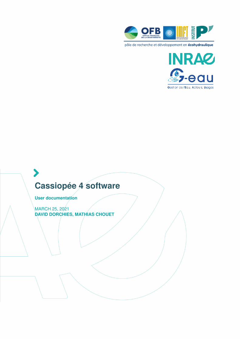
Figure 1.1: Top banner of the application with the menu, the list of open modules and thebutton to add a new module
The list of modules is available when the application is launched. After opening a newcalculation module, this list is available via the “+” button located in the upper banner or viathe “” menu and then the “New calculation module” link located in the menu.
The list of open modules appears in the upper banner and allows you to navigate betweenopen modules.
1.1.2.2 How are the choices made to perform a calculation or a series of calculations ?
The module is presented as a series of parameters involved in solving the equation of thecalculation module.
For each of them, the user can choose to:
• Set the parameter’s value (“FIXED” button);
• Vary the parameter to perform a series of calculations (“VARIATED” button);
• Choose the parameter that will be calculated (“CALCULATE” button).
The interface is designed so that one and only one parameter is chosen for the calcula-tion. Parameters that cannot be calculated do not have a “CALCULATE” button.
1.1.2.3 How to vary a parameter to perform a series of calculations
A series of calculations can be triggered between a minimum value and a maximum valuefor a given step:
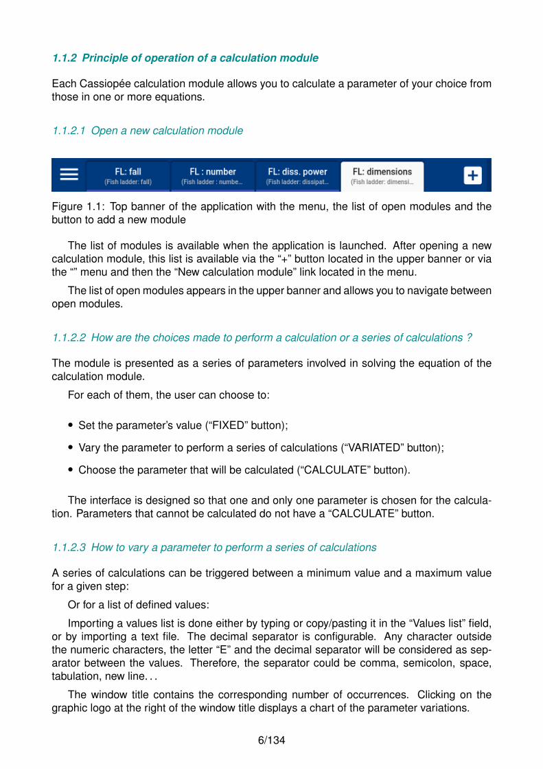
Or for a list of defined values:
Importing a values list is done either by typing or copy/pasting it in the “Values list” field,or by importing a text file. The decimal separator is configurable. Any character outsidethe numeric characters, the letter “E” and the decimal separator will be considered as sep-arator between the values. Therefore, the separator could be comma, semicolon, space,tabulation, new line. . .
The window title contains the corresponding number of occurrences. Clicking on thegraphic logo at the right of the window title displays a chart of the parameter variations.
6/134

Figure 1.2: Parameters of the module for calculating the fall of a basin pass
In case several parameters vary and they do not have the same number of occurrences,it is necessary to define a strategy to extend the shortest lists to fit the list of the parameterwith the most occurrences. Two strategies are available: repeat the last value or reuse thevalues in the list since the first occurrence.
1.1.2.4 How to launch a calculation or a series of calculations
Press the [Enter] key or click on the “Calculate” button at the bottom of the page.
1.1.2.5 Calculation results
For fixed parameters, the results panel displays the fixed parameters and the calculatedparameter as well as any additional results.
7/134

Figure 1.3: Define min, max and step values for a parameter to be varied
For one or more varying parameters, the results panel displays:
• an evolution graph on the which you can choose the parameter to use on the x-axisand y-axis;
• a table containing the parameters set;
• a table showing the parameters that vary and the calculated parameter as well as thevalues of any additional results.
The tables and charts are provided with different functionalities:
• a download button to retrieve the table content in XLSX format;
• a download button to retrieve the chart in PNG format;
• a button to display the table or chart in full screen.
The charts are zoomed in by making a mouse selection on some area. The button withthe curved left-pointing arrow resets the zoom to its original position displaying all availablevalues.
8/134
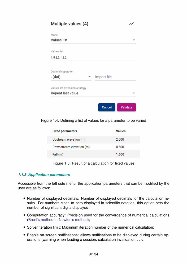
Figure 1.4: Defining a list of values for a parameter to be varied
Figure 1.5: Result of a calculation for fixed values
1.1.3 Application parameters
Accessible from the left side menu, the application parameters that can be modified by theuser are as follows:
• Number of displayed decimals: Number of displayed decimals for the calculation re-sults. For numbers close to zero displayed in scientific notation, this option sets thenumber of significant digits displayed;
• Computation accuracy: Precision used for the convergence of numerical calculations(Brent’s method or Newton’s method);
• Solver iteration limit: Maximum iteration number of the numerical calculation;
• Enable on-screen notifications: allows notifications to be displayed during certain op-erations (warning when loading a session, calculation invalidation. . . );
9/134
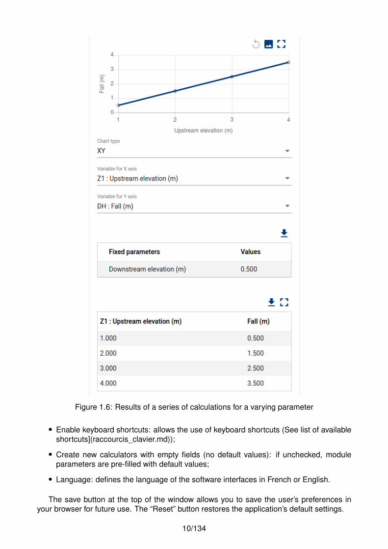
Figure 1.6: Results of a series of calculations for a varying parameter
• Enable keyboard shortcuts: allows the use of keyboard shortcuts (See list of availableshortcuts](raccourcis_clavier.md));
• Create new calculators with empty fields (no default values): if unchecked, moduleparameters are pre-filled with default values;
• Language: defines the language of the software interfaces in French or English.
The save button at the top of the window allows you to save the user’s preferences inyour browser for future use. The “Reset” button restores the application’s default settings.
10/134
1.1.4 Keyboard shortcuts list
To use keyboard shortcuts, the feature must be enabled in [application parameters.
• Alt + S: Saves the current session
• Alt + O: Opens a session file
• Alt + Q: Empties the current session
• Alt + N: Adds a new calculation module to the current session
• Alt + : Triggers calculation of the current module
• Alt + D: Duplicates the current module
• Alt + W: Closes the current module
• Alt + G: Shows modules diagram
• Alt + 1: Positions the page on the “Input” section of the current module
• Alt + 2: Positions the page on the “Results” section of the current module
• Alt + 3: Positions the page on the “Charts” section of the current module
1.2 Pipe flow
1.2.1 Lechapt and Calmon
This module allows to calculate the pressure losses in a circular pipe from the Lechapt andCalmon abacuses.
It allows the calculation of the value of one of the following quantities:
• Flow rate (m3/s)
• Pipe diameter (m)
• Total head loss (m)
• Pipe length (m)
• Singular pressure loss coefficient (m)
The total head loss is the sum of the linear head losses JL obtained from the Lechaptand Calmon abacuses and singular JS depending on the above coefficient.
11/134

1.2.1.1 Lechapt and Calmon abacuses
Lechapt and Calmon formula is based on adjustements of Cyril Frank Colebrook formula:
JL =lT
1000L.QM .D−N
With:
• JL: headloss in mm/m or m/km;
• lT : pipe length in m;
• Q: flow in L/s;
• D: pipe diameter in m;
• L, M and N coefficients depending on roughness {}.
The error made with respect to the Colebrook formula is less than 3% for speeds between0.4 and 2 m/s.
The correlation table of the coefficients is as follows:
Table 1.1: Materials and coefficients used in the Lechapt and Calmon formula
Material (mm) L M N
Uncoated cast iron or steel - Coarse concrete(corrosive water)
2 1.863 2 5.33
Uncoated cast iron or steel - Coarse concrete(low corrosive water)
1 1.601 1.975 5.25
Cast iron or steel with cement coating 0.5 1.40 1.96 5.19Cast iron or steel bitumen coating - centrifugedconcrete
0.25 1.16 1.93 5.11
Rolled steel - smooth concrete 0.1 1.10 1.89 5.01Cast iron or steel centrifugal coating 0.05 1.049 1.86 4.93PVC - polyethylene 0.025 1.01 1.84 4.88Hydraulically smooth pipe - 0.05 D 0.2 0.00 0.916 1.78 4.78Hydraulically smooth pipe - 0.25 D 1 0.00 0.971 1.81 4.81
1.2.1.2 Singular head loss
JS = KSV 2
2g
With:
• KS : singular head loss coefficient
• V : water speed in the pipe (V = 4Q/π/D2)
12/134

1.2.1.3 Darcy’s head loss coefficient
$$ f_D = 2g J DlTV 2
1.2.2 Distributor pipe
Analytical relationship for the direct calculation of pressure drops in pipes distributing a flowrate in a homogeneous manner based on the Blasius formula.
1.2.2.1 Assumptions
Figure 1.7: Conduct diagram
We assume a pipe length L, inner diameter D, with a flow rate at the top Q. We calculatethe pressure drop between the two ends of the pipe. In a constant flow section q, the frictioncoefficient is evaluated with the Blasius formula, valid for moderate Reynolds numbers forsmooth walls:
λ ' aRe−0.25
1.2.2.2 Analytical development
We’re recording the position from the downstream end of the pipe. The flow rate is supposedto vary linearly with x, and is then written:
q(x) = Qx/L
Let’s note S = πD2/4 the inner surface of the pipe. The pressure drop is obtained byintegrating the Darcy-Weisbach relationship:
∆H =
∫ L
x=0
aRe−0.25u2(x)
2gDdx
Note the kinematic viscosity. We then replace Re with uD/ν, which gives
∆H =
∫ L
x=0
au(x)−0.25D−0.25ν0.25u2(x)
2gDdx
By rearranging, we get:
∆H =
∫ L
x=0
aν0.25u1.75(x)
2gD1.25dx
13/134

Let’s use the flow equation to show the flow (u(x) = q(x)/S):
∆H =
∫ L
x=0
aν0.25(Qx/(LS))1.75
2gD1.25dx
then the diameter:
∆H =
∫ L
x=0
aν0.25(4Qx/(LπD2))1.75
2gD1.25dx
We rearrange to get
∆H = aν0.25(4/π)1.75Q1.75
2gD4.75
∫ L
x=0
(x/L)1.75dx
By integrating, we obtain
∆H = aν0.25(4/π)1.75Q1.75
2gD4.75
L
2.75
∆H = aν0.2541.75
5.5gπ1.75Q1.75LD4.75
1.2.2.3 Digital application
For water at 20°C: ν ' 10−6 m2/s, which gives
DeltaH = 0.323 10−3Q1.75
D4.75L
with ∆H in meters.
For water at 50°C, ν ' 0.55610−6 m2/s, which means that the pressure drop is reducedby about 14%, or
DeltaH = 0.28 10−3Q1.75
D4.75L
1.3 Open-channel flow
1.3.1 Uniform flow
The uniform flow is characterized by a water height called the normal height. The normalheight is reached when the water line is parallel to the bottom, the load is then itself parallelto the water line and thus the head loss is equal to the slope of the bottom: If = J
With:
• If : bottom slope in m/m
14/134

• J : head loss in m/m
The head loss {J} is calculated here using Manning-Strickler’s formula:
J =U2
K2R4/3=
Q2
S2K2R4/3
With:
• K: Strickler coefficient in m1/3/s
In uniform flow, we obtain the formula:
Q = KR2/3S√If
Based on the which, flow Q, slope If and Strickler calculation K can be calculated ana-lytically.
To calculate normal height hn , one can solve f(hn) = Q−KR2/3S√If = 0
using Newton’s method:
hk+1 = hk −f(hk)
f ′(hk)
with:
• f(hk) = Q−KR2/3S√If
• f ′(hk) = −K√If (
23R′R−1/3S +R2/3S ′)
To calculate the geometrical parameters of the section, the calculation module uses theflow calculation equation and solves the problem by dichotomy.
1.3.2 Backwater curve
The calculation of the backwater curve involves the following differential equation:
dy
dx=If − J(h)
1− F 2(h)
where If is the slope of a canal, J the formula giving us the local pressure drop (depend-ing on the water level), y here refers to the height of water.
Thus, for a rectangular channel of width b and a Strickler coefficient K:
J =Q2(b+ 2y)4/3
K2b10/3y10/3
and
15/134
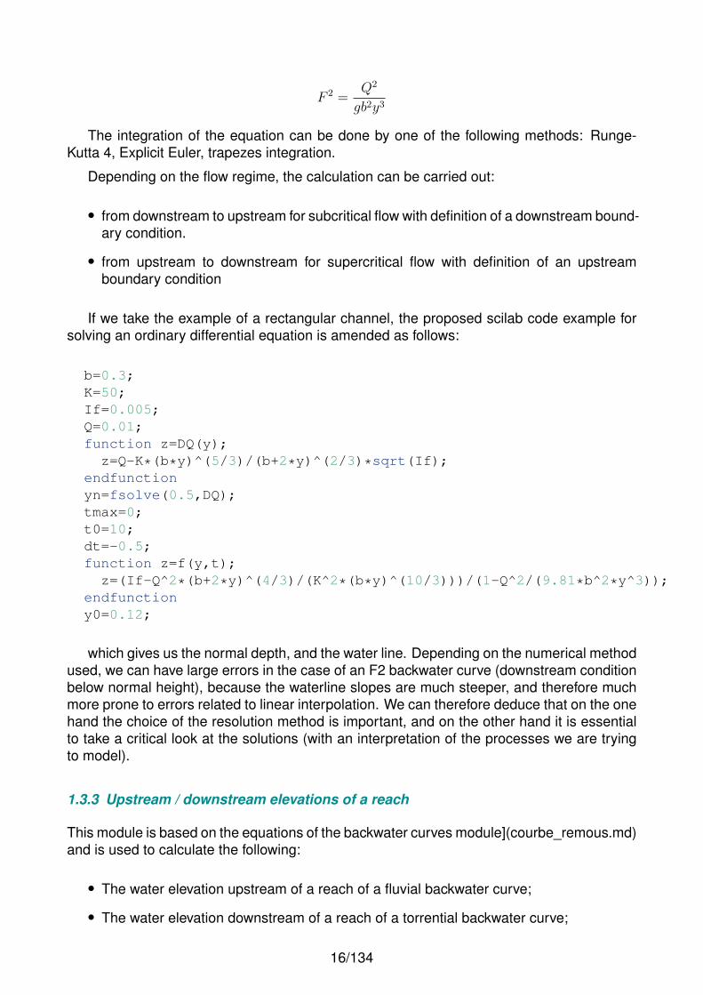
F 2 =Q2
gb2y3
The integration of the equation can be done by one of the following methods: Runge-Kutta 4, Explicit Euler, trapezes integration.
Depending on the flow regime, the calculation can be carried out:
• from downstream to upstream for subcritical flow with definition of a downstream bound-ary condition.
• from upstream to downstream for supercritical flow with definition of an upstreamboundary condition
If we take the example of a rectangular channel, the proposed scilab code example forsolving an ordinary differential equation is amended as follows:
b=0.3;K=50;If=0.005;Q=0.01;function z=DQ(y);
z=Q-K*(b*y)^(5/3)/(b+2*y)^(2/3)*sqrt(If);endfunctionyn=fsolve(0.5,DQ);tmax=0;t0=10;dt=-0.5;function z=f(y,t);
z=(If-Q^2*(b+2*y)^(4/3)/(K^2*(b*y)^(10/3)))/(1-Q^2/(9.81*b^2*y^3));endfunctiony0=0.12;
which gives us the normal depth, and the water line. Depending on the numerical methodused, we can have large errors in the case of an F2 backwater curve (downstream conditionbelow normal height), because the waterline slopes are much steeper, and therefore muchmore prone to errors related to linear interpolation. We can therefore deduce that on the onehand the choice of the resolution method is important, and on the other hand it is essentialto take a critical look at the solutions (with an interpretation of the processes we are tryingto model).
1.3.3 Upstream / downstream elevations of a reach
This module is based on the equations of the backwater curves module](courbe_remous.md)and is used to calculate the following:
• The water elevation upstream of a reach of a fluvial backwater curve;
• The water elevation downstream of a reach of a torrential backwater curve;
16/134

• The flow that connects the upstream and downstream water elevations of a fluvial ortorrential backwater curve.
The regime chosen on the type of water line determines whether the calculation is madefrom downstream to upstream (fluvial regime) and from upstream to downstream (torrentialregime).
This calculation module is particularly useful for calculating the water line of a series ofhydraulic structures or reaches (see the typical example “Flow of a channel with structures”).
1.3.4 Parametric section
This module calculates the hydraulic quantities associated to:
• a section with a defined geometrical shape ([See section types managed by Cas-siopée)
• a draft y in m
• a flow Q in m3/s
• a bottom slope If in m/m
• a roughness expressed with the Strickler’s coefficient K in m1/3/s
The calculated hydraulic quantities are:
• Width at mirror (m)
• Wet perimeter (m)
• Hydraulic surface (m2)
• Hydraulic radius (m)
• Average speed (m/s)
• Specific head (m)
• Head loss (m)
• Linear variation of specific energy (m/m)
• Normal depth (m)
• Froude number
• Critical depth (m)
• Critical head (m)
• Corresponding depth (m)
• Impulsion (kgms-1)
• Conjugate depth
• Tractive force (Pa)
17/134
1.3.4.1 Bank height, overflow and closed-conduit flow
The sections are all provided with a bank height which is used at three levels in the freesurface hydraulics calculation tools:
• It allows to define if the calculated water level overflows the section.
• Beyond this bank height the hydraulic calculations simulate a flow between two verticalwalls. For example, a semi-circular pipe can be modelled by defining a bank heightequal to the radius of the pipe.
• For a circular pipe, a bank height greater than or equal to the diameter of the pipemakes it possible to model a closed pipe. If the water level exceeds the diameter of thepipe, hydraulic calculations simulate a closed-conduit flow using the Preissmann slottechnique.
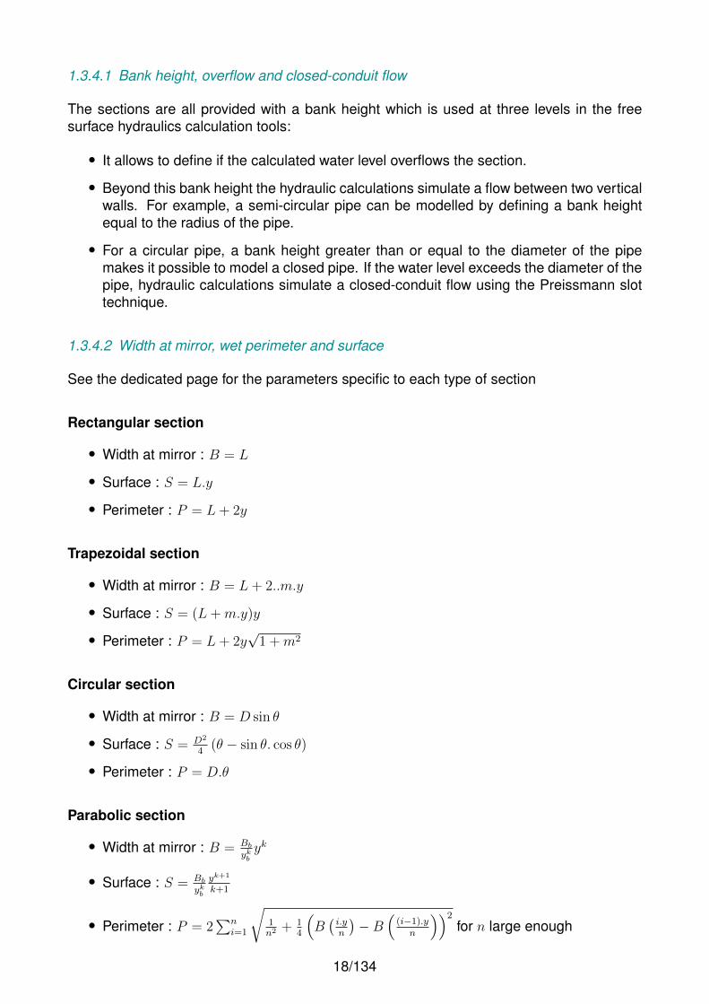
1.3.4.2 Width at mirror, wet perimeter and surface
See the dedicated page for the parameters specific to each type of section
Rectangular section
• Width at mirror : B = L
• Surface : S = L.y
• Perimeter : P = L+ 2y
Trapezoidal section
• Width at mirror : B = L+ 2..m.y
• Surface : S = (L+m.y)y
• Perimeter : P = L+ 2y√
1 +m2
Circular section
• Width at mirror : B = D sin θ
• Surface : S = D2
4(θ − sin θ. cos θ)
• Perimeter : P = D.θ
Parabolic section
• Width at mirror : B = Bb
ykbyk
• Surface : S = Bb
ykb
yk+1
k+1
• Perimeter : P = 2∑n
i=1
√1n2 + 1
4
(B(i.yn
)−B
((i−1).yn
))2for n large enough
18/134

1.3.4.3 Hydraulic radius (m)
R = S/P
1.3.4.4 Average speed (m/s)
U = Q/S
1.3.4.5 Specific head (m)
H(y) = y +U2
2g
1.3.4.6 Head loss (m/m)
Cassiopée uses Manning Strickler formula:
J =U2
K2R4/3=
Q2
S2K2R4/3
1.3.4.7 Linear variation of specific energy (m/m)
∆Es = If − J
1.3.4.8 Normal depth (m)
See the uniform flow calculation.
1.3.4.9 Froude number
The Froude number expresses the ratio between the mean fluid velocity and the surfacewave velocity. c.
c =
√gS
B
Fr =U
c=
√Q2B
gS3
1.3.4.10 Critical depth (m)
The critical height is reached when the average velocity of the fluid is equal to the velocity ofthe waves on the water surface.
The critical height is therefore reached when the Froude number Fr = 1.
For any section, the critical height is calculated as follows yc by solving f(yc) = Fr2−1 = 0
19/134
We use Newton’s method by posing yk+1 = yk − f(yk)f ′(yk)
with : - f(yk) = Q2BgS3 − 1 - f ′(yk) =
Q2
gB′.S−3BS′
S4
1.3.4.11 Critical head (m)
This is the head calculated for a draft equal to the critical depth. Hc = H(yc).
1.3.4.12 Corresponing depth (m)
For a fluvial (respectively torrential draft) y, corresponding depth is the torrential (respectivelyfluvial) draft for the which H(y) = H(ycor).
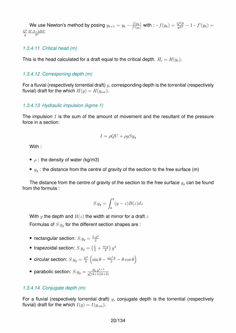
1.3.4.13 Hydraulic impulsion (kgms-1)
The impulsion I is the sum of the amount of movement and the resultant of the pressureforce in a section:
I = ρQU + ρgSyg
With :
• ρ : the density of water (kg/m3)
• yg : the distance from the centre of gravity of the section to the free surface (m)
The distance from the centre of gravity of the section to the free surface yg can be foundfrom the formula :
S.yg =
∫ y
0
(y − z)B(z)dz
With y the depth and B(z) the width at mirror for a draft z
Formulas of S.yg for the different section shapes are :
• rectangular section: S.yg = L.y2
2
• trapezoidal section: S.yg =(L2
+ m.y3
)y2
• circular section: S.yg = D3
8
(sin θ − sin3 θ
3− θ cos θ
)• parabolic section: S.yg = Bb.y
k+2
ykb (k+1)(k+2)
1.3.4.14 Conjugate depth (m)
For a fluvial (respectively torrential draft) y, conjugate depth is the torrential (respectivelyfluvial) draft for the which I(y) = I(ycon).
20/134

1.3.4.15 Tractive force (Pa)
τ0 = ρgRJ
1.3.5 Slope
1.3.5.1 Definition
The slope used in all Cassiopée’s modules is the topographic slope:
The grade (also called slope, incline, gradient, mainfall, pitch or rise) of a physicalfeature, landform or constructed line refers to the tangent of the angle of thatsurface to the horizontal. (Source: Wikipedia)
Figure 1.8: Longitudinal cross-sectional scheme of a rectilinear section
The slope (I) in m/m used in Cassiopee’s modules is:
I = ∆h/d = tan(α)
Important:
All calculation modules consider a descending slope as positive except for the “Jet Im-pact” module where a positive slope will be considered as rising and vice versa. To invertthe slope in a calculation sequence of linked modules, use the “linear function” module witha = −1 and b = 0.
1.3.5.2 The “Slope” module
This tools allows to calculate the missing value of the four quantities:
• upstream elevation (Z1) in m;
• downstream elevation (Z2) in m;
• length (d) in m;
• slope (I) in m/m, with I = (Z1−Z2)d
.
1.3.6 Section types
1.3.6.1 Rectangular section
The rectangular section is characterized by the following parameters:
• width at bottom L (in m)
21/134

Figure 1.9: Rectangular section
Figure 1.10: Circular section
1.3.6.2 Circular section
The circular section is characterized by the following parameters:
• the pipe diameter D (in m)
• the angle θ between the pipe bottom and the junction point between water surface andpipe (in Rad)
θ = arccos(
1− yD/2
)θ′ = 2
D√
1−(1− 2yD )
2
1.3.6.3 Trapezoidal section
Figure 1.11: Trapezoidal section
The trapezoidal section is characterized by the following parameters:
• width at bottom L (in m)
• bank slope (inclination to the vertical: widening between the top and bottom of theslope divided by the depth.) m (in m/m)
1.3.6.4 Parabolic section
The parabolic section is characterized by a mirror width that can be expressed in the form:
B = Λ.yk.
With k: coefficient between 0 and 1. k = 0.5 corresponds to the true parabolic form.
Λ can be calculated by giving:
• yb: bank height (in m)
22/134

• Bb: embankment width (in m)
We then have: Λ = Bb
ykb
1.3.7 Manning-Strickler’s formula
1.3.7.1 Definition
Manning-Strickler formula is written as follows:
V = KsR2/3h i1/2
with:
• V la vitesse moyenne de la section transversale en m/s
• Ks Strickler’s coefficient
• Rh Hydraulic radius in m
• i slope en m/m
The Strickler coefficient Ks varies from 20 (rough stone and rough surface) to 80 (smoothconcrete and cast iron).
Manning’s coefficient n is obtained by :
n =1
Ks
1.3.7.2 Chow’s table (1959)
Table 1.2: Chow’s table (1959)
Type of channel and description KS min. KS normal KS max.
1. Main channelsa. clean, straight, full stage, no rifts or deeppools
30 33 40
b. same as above, but more stones andweeds
25 29 33
c. clean, winding, some pools and shoals 22 25 30d. same as above, but some weeds andstones
20 22 29
e. same as above, lower stages, moreineffective slopes and sections
18 21 25
f. same as “d” with more stones 17 20 22g. sluggish reaches, weedy, deep pools 13 14 20h. very weedy reaches, deep pools, orfloodways with heavy stand of timber andunderbrush
7 10 13
23/134

Type of channel and description KS min. KS normal KS max.
2. Mountain streams, no vegetation inchannel, banks usually steep, trees andbrush along banks submerged at highstagesa. bottom: gravels, cobbles, and few boulders 20 25 33b. bottom: cobbles with large boulders 14 20 253. Floodplainsa. Pasture, no brush1. short grass 29 33 402. high grass 20 29 33b. Cultivated areas1. no crop 25 33 502. mature row crops 22 29 403. mature field crops 20 25 33c. Brush1. scattered brush, heavy weeds 14 20 292. light brush and trees, in winter 17 20 293. light brush and trees, in summer 13 17 254. medium to dense brush, in winter 9 14 225. medium to dense brush, in summer 6 10 14d. Trees1. dense willows, summer, straight 5 7 92. cleared land with tree stumps, no sprouts 20 25 333. same as above, but with heavy growth ofsprouts
13 17 20
4. heavy stand of timber, a few down trees,little undergrowth, flood stage belowbranches
22 21 20
5. same as 4. with flood stage reachingbranches
6 8 10
4. Excavated or Dredged Channelsa. Earth, straight, and uniform1. clean, recently completed 50 56 632. clean, after weathering 40 45 563. gravel, uniform section, clean 33 40 454. with short grass, few weeds 30 37 45b. Earth winding and sluggish1. no vegetation 33 40 432. grass, some weeds 30 33 403. dense weeds or aquatic plants in deepchannels
25 29 33
4. earth bottom and rubble sides 29 33 365. stony bottom and weedy banks 25 29 406. cobble bottom and clean sides 20 25 33c. Dragline-excavated or dredged1. no vegetation 30 36 402. light brush on banks 17 20 29d. Rock cuts1. smooth and uniform 25 29 40
24/134
Type of channel and description KS min. KS normal KS max.
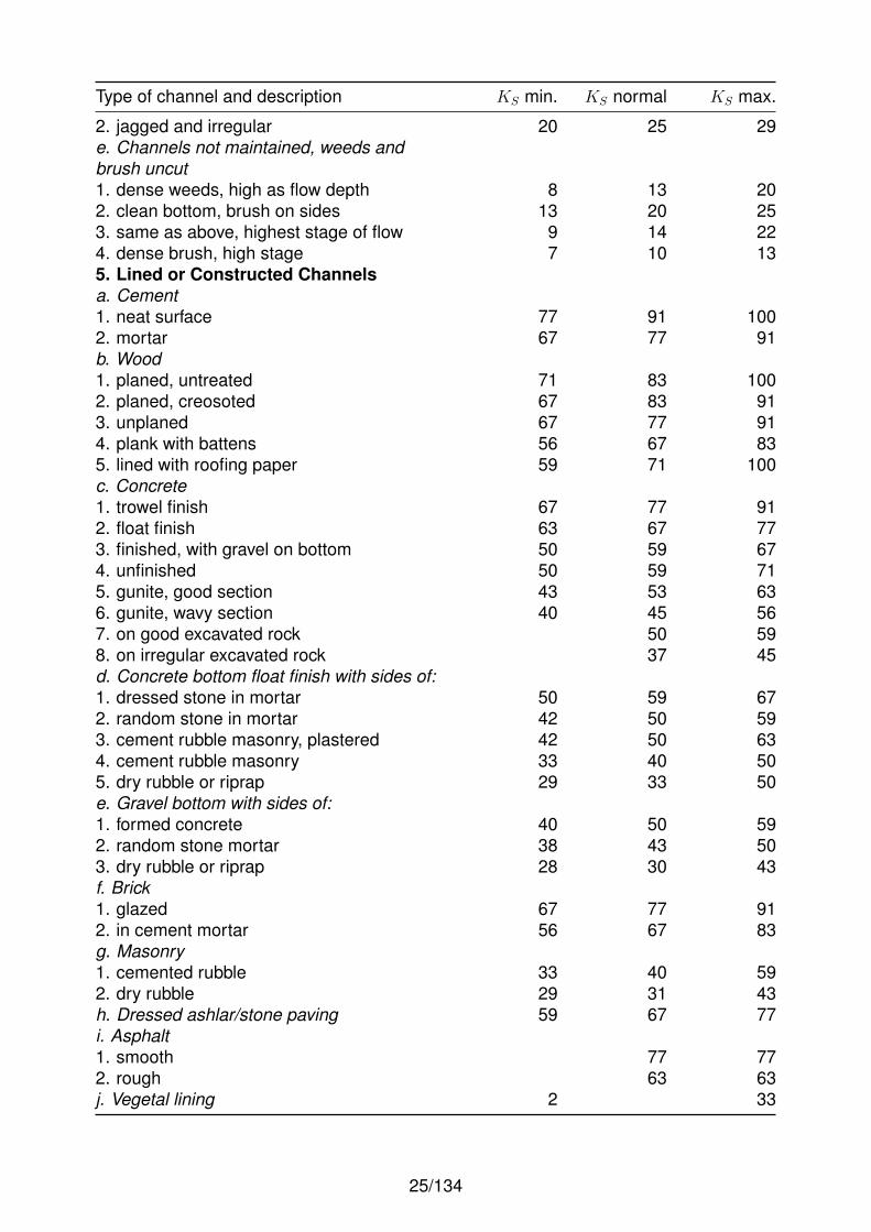
2. jagged and irregular 20 25 29e. Channels not maintained, weeds andbrush uncut1. dense weeds, high as flow depth 8 13 202. clean bottom, brush on sides 13 20 253. same as above, highest stage of flow 9 14 224. dense brush, high stage 7 10 135. Lined or Constructed Channelsa. Cement1. neat surface 77 91 1002. mortar 67 77 91b. Wood1. planed, untreated 71 83 1002. planed, creosoted 67 83 913. unplaned 67 77 914. plank with battens 56 67 835. lined with roofing paper 59 71 100c. Concrete1. trowel finish 67 77 912. float finish 63 67 773. finished, with gravel on bottom 50 59 674. unfinished 50 59 715. gunite, good section 43 53 636. gunite, wavy section 40 45 567. on good excavated rock 50 598. on irregular excavated rock 37 45d. Concrete bottom float finish with sides of:1. dressed stone in mortar 50 59 672. random stone in mortar 42 50 593. cement rubble masonry, plastered 42 50 634. cement rubble masonry 33 40 505. dry rubble or riprap 29 33 50e. Gravel bottom with sides of:1. formed concrete 40 50 592. random stone mortar 38 43 503. dry rubble or riprap 28 30 43f. Brick1. glazed 67 77 912. in cement mortar 56 67 83g. Masonry1. cemented rubble 33 40 592. dry rubble 29 31 43h. Dressed ashlar/stone paving 59 67 77i. Asphalt1. smooth 77 772. rough 63 63j. Vegetal lining 2 33
25/134
1.4 Parallel structures
1.4.1 Parallel structures
1.4.1.1 Description of the calculation module
This calculation module allows to simulate the hydraulic operation of valves and thresholdsplaced in parallel. All the flow laws present in Cassiopée are grouped in this module, whichmakes it possible in particular to easily compare the flow laws between them.
This module allows to calculate any missing parameter among them:
• Boundary conditions (water level upstream and downstream of the structures);
• The flow through the structures;
• Parameters of the structures (crest elevation, width, flow coefficient. . . ).
The module calculates the requested parameter and displays for each structure present:
• The flow passing through the structure;
• The type of flow: under load (flow pinched under a gate), or free surface;
• The speed: flooded, partially flooded or dewatered;
• The type of jet for free surface flows: surface or submerged.
1.4.1.2 Jet type
For the definition of the type of jet (plunging or surface), see: Larinier, M., 1992. Succes-sive basin transitions, pre-dams and artificial rivers. Bulletin Français de la Pêche et de laPisciculture 45-72. https://doi.org/10.1051/kmae:1992005.
Excerpt from Larinier, M., 1992. Passages to successive basins, pre-dams and artificialrivers. Bulletin Français de la Pêche et de la Pisciculture 45-72. https:// doi.org/ 10.1051/kmae:1992005
The definition used in Cassiopée is as follows:
• if DH ≥ 0.5H1 then the jet is plunging;
• if DH < 0.5H1 then the jet is surface.
With H1, the upstream head over the weir and DH the head drop across the weir.
26/134

Figure 1.12: Diagram of jet type
1.4.2 Free flow weir stage-discharge laws
This calculation module is similar to that of the Parallel structures, except that it simulatesonly free flows and refine by using the upstream approach speed.
It can be used to calculate the relationship between water level upstream of a weir andflow. It is most often used to assess the upstream-flow rating relationship at a weir or struc-ture evacuator of a development. The facility may have several distinct discharge levels andRectangular (with horizontal discharge side), triangular, semi-triangular weirs or truncatedtriangles.
The classical use consists in entering the extreme levels (min/max) of the upstream waterlevel and the calculation step for which flow estimates are desired.
The upstream characteristics (upstream width and bed elevation) make it possible toestimate the approach speed and upstream kinetic energy, expressed in metres, and tocalculate total flow from the total head at a non-negligible approach speed.
V =Q
L× (Z1 − Zlit)
with V the approach speed, Q the flow, Z1 the upstream water elevation, Zlit the up-stream river bed elevation.
27/134

Ec =V 2
2g
with Ec the upstream cinetic energy in metres, and g the acceleration of gravity (9.81m.s-2).
Head H used for flow calculation then is:
H = Z1 + Ec
The difficulty of the calculation lies in the fact that the flow rate to be calculated is involvedin the calculation of the head. This problem is solved with the fixed point algorithm wherethe flow rate calculation is repeated several times by updating the head at each iteration untilthe calculation converges to the final value of the flow rate.
The approach speed correction coefficient Cv is then calculated by relating the flow rateobtained with the head H to the flow rate calculation with the upstream dimension Z1.
1.4.3 Cross walls
This tool, which is similar to the Parallel Structures tool, is an aid to the hydraulic pre-dimensioning of a fish pass: it is most often used for the dimensioning of notches, slots,orifices, etc. characterizing the walls of a pass as well as for the setting in altitude of thenotches, slots and apron of the upstream basin of a pass.
It allows to calculate the missing value of the 7 values characterizing the fall, the surfaceof the submerged orifice, the width of the slot, the load on the slot, the width of the notch,the load on the notch and the flow rate.
Mandatory data to be provided are the dimensions of the basins (width and length) andthe average draught in metres. These data associated with the fall between basins allow usto calculate the power dissipation.
Once the module is calculated, the tool proposes to create a basin pass from this crosswall by specifying the upstream water elevation, the number of falls in the pass and thedownstream water elevation.
1.4.3.1 Hydraulic structures that can be part of the cross wall
The tool allows you to place one or more structures in parallel among the following types ofstructures:
Submerged orifice Excerpt from Larinier, M., Travade, F., Porcher, J.-P., Gosset, C., 1992.Fish passage: expertise and design of crossing structures. CSP. (page 94).
The submerged orifice equation is described on the submerged orifice formula page.
Submerged Slot Excerpt from Larinier, M., Travade, F., Porcher, J.-P., Gosset, C., 1992.Fish passage: expertise and design of crossing structures. CSP. (page 94).
The submerged slot equation is described on the sumberged slot formula page.
28/134

Figure 1.13: Submerged orifice diagram
Figure 1.14: Schematic of the submerged slot
Notch Excerpt from Larinier, M., Travade, F., Porcher, J.-P., Gosset, C., 1992. Fish pas-sage: expertise and design of crossing structures. CSP. (page 94).
The equation used for the notch is that of Kindsvater-Carter and Villemonte.
29/134

Figure 1.15: Notch diagram
1.4.4 Device equations
1.4.4.1 Stage-discharge equations list
Table 1.3: Stage-discharge equations list
EquationDefault discharge
coefficient Available in
Broad-crested weir / Orifice(Cemagref-D)
0.4 Parallel Structures
Broad-crested weir / sluicegate (Cemagref-V)
0.6 Parallel Structures
Broad-crested weir / orifice(Cunge)
0.6 Parallel Structures, Cross walls,Downwall
Free flow sluice gate 0.6 Parallel StructuresSubmerged sluice gate 0.8 Parallel StructuresFree flow sharp-crested weir(Poleni)
0.4 Parallel Structures, Free flow weirstage-discharge laws
Deeply submergedsharp-crested weir(Rajaratnam)
0.9 Parallel Structures
Submerged slot (Larinier) 0.75 Parallel Structures, Cross walls,Downwall
Sharp-crested weir(Kindsvater-Carter +Villemonte)
α=0.4, β=0.001 Parallel Structures
30/134
EquationDefault discharge
coefficient Available in
Triangular weir sharp-crested(Villemonte) andbroad-crested (Bos)
1.36 Parallel Structures, Free flow weirstage-discharge laws, Cross walls,Downwall
Truncated triangular weir(Villemonte)
1.36 Parallel Structures, Free flow weirstage-discharge laws, Cross walls,Downwall
Submerged orifice (Bernoulli) 0.7 Parallel Structures, Cross walls,Downwall
Free flow orifice (Bernoulli) 0.7 Parallel StructuresSharp-crested weir(Villemonte)
0.4 Parallel Structures, Cross walls,Downwall
Regulated notch (Villemonte) 0.4 DownwallRegulated submerged slot(Larinier)
0.75 Downwall
1.4.4.2 Kindsvater-Carter and Villemonte formula
The calculation module allows hydraulic calculations to be carried out for several structuresin parallel.
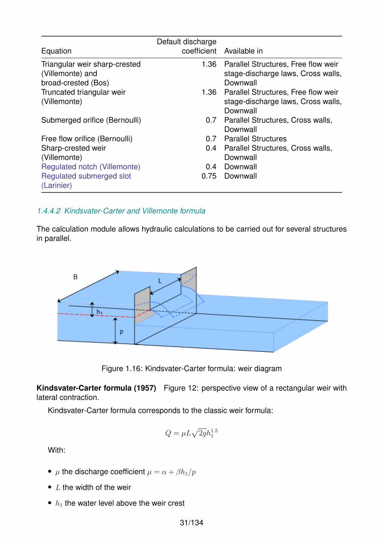
Figure 1.16: Kindsvater-Carter formula: weir diagram
Kindsvater-Carter formula (1957) Figure 12: perspective view of a rectangular weir withlateral contraction.
Kindsvater-Carter formula corresponds to the classic weir formula:
Q = µL√
2gh1.51
With:
• µ the discharge coefficient µ = α + βh1/p
• L the width of the weir
• h1 the water level above the weir crest
31/134

• p the sill or weir crest height
The coefficients α and β depend on the ratio between the width of the weir (L) andthe width of the basin (B). Their values are given in the abacuses below (Excerpt fromLarinier, M., Porcher, J.-P., 1986. Programmes de calcul sur HP86 : hydraulique et passes àpoissons):
Figure 1.17: Kindsvater-Carter formula: abacuses
Submerged flow: Villemonte formula (1947) For a downstream water elevation higherthan the elevation of the weir crest, the flow is submerged and a flooding coefficient is appliedto the flow coefficient.
Villemonte proposes the following formula:
K =Qsubmerged
Qfree
=
[1−
(h2
h1
)n]0.385With: - h1 the upstream water level above the weir crest - h2 the downstream water level
above the weir crest - n the exponent in free flow relationships (rectangular=1.5, triangu-lar=2.5, parabolic=2)
32/134
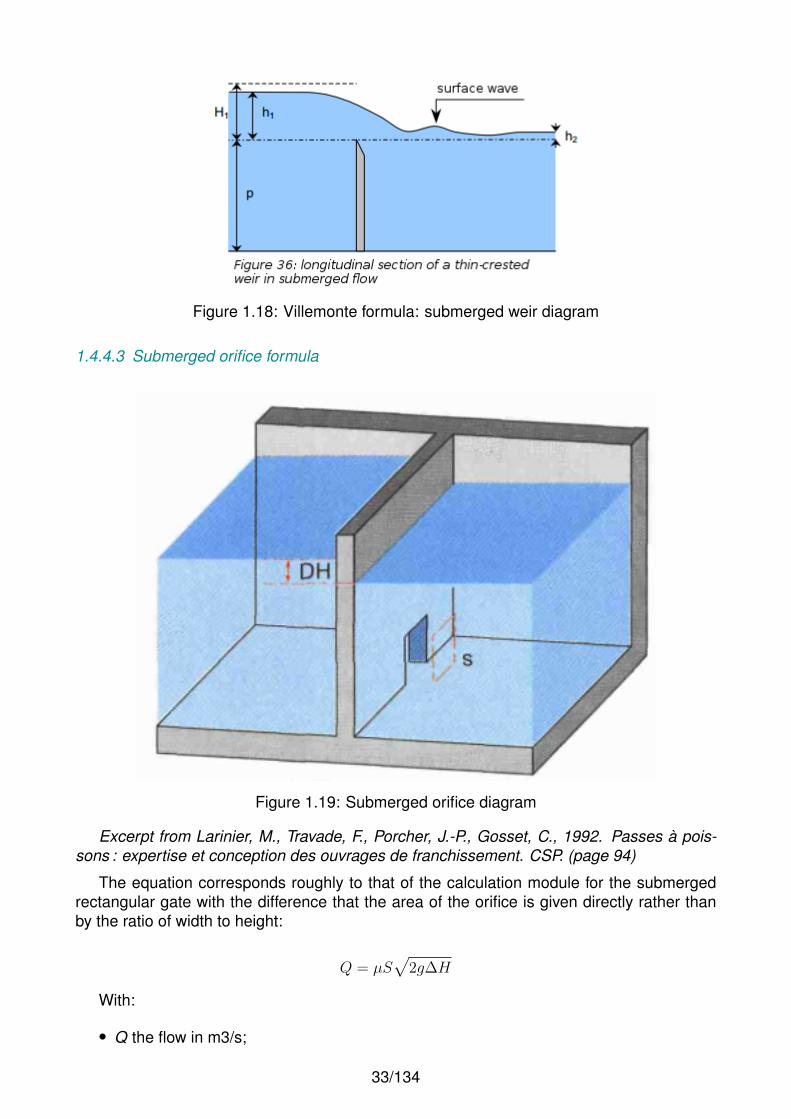
Figure 1.18: Villemonte formula: submerged weir diagram
1.4.4.3 Submerged orifice formula
Figure 1.19: Submerged orifice diagram
Excerpt from Larinier, M., Travade, F., Porcher, J.-P., Gosset, C., 1992. Passes à pois-sons : expertise et conception des ouvrages de franchissement. CSP. (page 94)
The equation corresponds roughly to that of the calculation module for the submergedrectangular gate with the difference that the area of the orifice is given directly rather thanby the ratio of width to height:
Q = µS√
2g∆H
With:
• Q the flow in m3/s;
33/134

• the discharge coefficient (equal to 0.7 by default);
• S the orifice surface in m2;
• H the head loss H1 - H2 in m(named “Fall” in Cassiopée).
1.4.4.4 Free orifice formula
Figure 1.20: Free orifice diagram
Excerpt from CARLIER, M. (1972). Hydraulique générale et appliquée. OCLC : 421635236.Paris : Eyrolles
The general formula for a free orifice or nozzle is as follows (CARLIER, 1972):
Q = CdS√
2gH
With:
• Q the flow in m3/s;
• Cd the discharge coefficient;
• S the orifice surface in m2;
• g the acceleration of gravity 9.81 m/s2
• H The water level measured from the surface of the water to the centre of the orificein meters.
The area S to be considered is the smallest cross-sectional area of the orifice or nozzle(Figure 5.12c). The discharge coefficient Cd varies depending on the type of orifice or nozzle.Figure 5.12 shows the most common shapes and discharge coefficients (Source: CARLIER,1972).
34/134
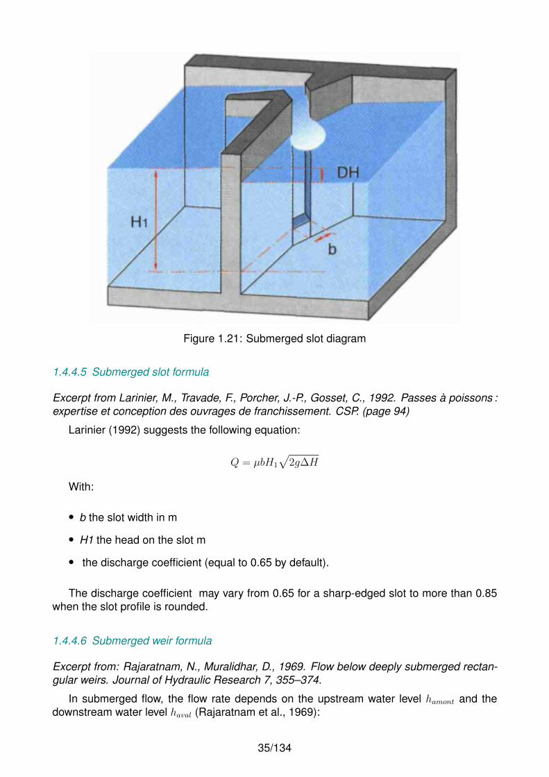
Figure 1.21: Submerged slot diagram
1.4.4.5 Submerged slot formula
Excerpt from Larinier, M., Travade, F., Porcher, J.-P., Gosset, C., 1992. Passes à poissons :expertise et conception des ouvrages de franchissement. CSP. (page 94)
Larinier (1992) suggests the following equation:
Q = µbH1
√2g∆H
With:
• b the slot width in m
• H1 the head on the slot m
• the discharge coefficient (equal to 0.65 by default).
The discharge coefficient may vary from 0.65 for a sharp-edged slot to more than 0.85when the slot profile is rounded.
1.4.4.6 Submerged weir formula
Excerpt from: Rajaratnam, N., Muralidhar, D., 1969. Flow below deeply submerged rectan-gular weirs. Journal of Hydraulic Research 7, 355–374.
In submerged flow, the flow rate depends on the upstream water level hamont and thedownstream water level haval (Rajaratnam et al., 1969):
35/134
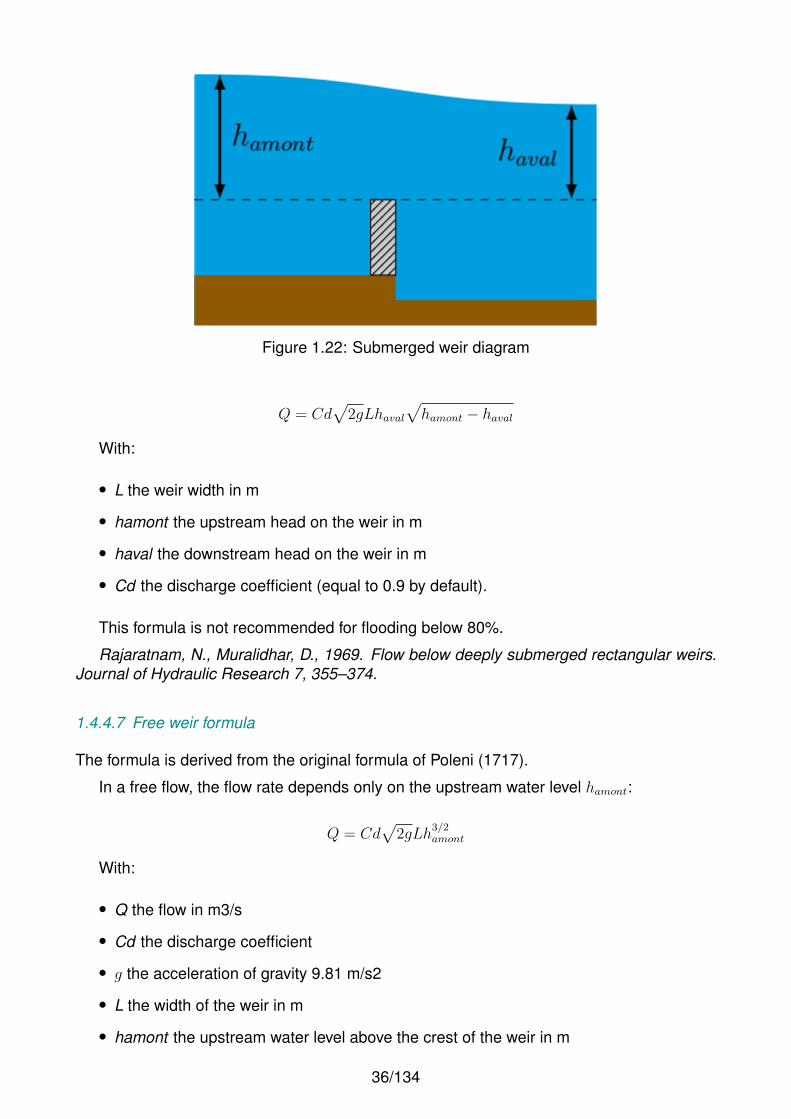
Figure 1.22: Submerged weir diagram
Q = Cd√
2gLhaval√hamont − haval
With:
• L the weir width in m
• hamont the upstream head on the weir in m
• haval the downstream head on the weir in m
• Cd the discharge coefficient (equal to 0.9 by default).
This formula is not recommended for flooding below 80%.
Rajaratnam, N., Muralidhar, D., 1969. Flow below deeply submerged rectangular weirs.Journal of Hydraulic Research 7, 355–374.
1.4.4.7 Free weir formula
The formula is derived from the original formula of Poleni (1717).
In a free flow, the flow rate depends only on the upstream water level hamont:
Q = Cd√
2gLh3/2amont
With:
• Q the flow in m3/s
• Cd the discharge coefficient
• g the acceleration of gravity 9.81 m/s2
• L the width of the weir in m
• hamont the upstream water level above the crest of the weir in m
36/134
A flow coefficient value Cd = 0.4 is generally a good approximation for a rectangularweir. For more complex weir shapes (trapezoidal, circular. . . ) or to take into account thecharacteristics of the longitudinal profile (thin-crested weir, thick-crested weir), one can referto the CETMEF weir leaflet (CETMEF, 2005).
CETMEF (2005). Notice sur les déversoirs : synthèse des lois d’écoulement au droit desseuils et déversoirs. Compiègne : Centre d’Études Techniques Maritimes Et Fluviales. 89 p.
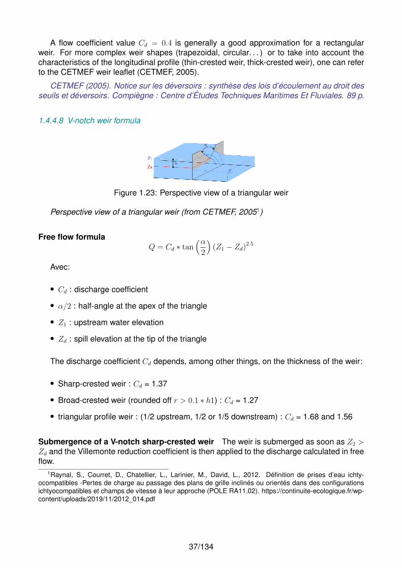
1.4.4.8 V-notch weir formula
Figure 1.23: Perspective view of a triangular weir
Perspective view of a triangular weir (from CETMEF, 20051)
Free flow formulaQ = Cd ∗ tan
(α2
)(Z1 − Zd)2.5
Avec:
• Cd : discharge coefficient
• α/2 : half-angle at the apex of the triangle
• Z1 : upstream water elevation
• Zd : spill elevation at the tip of the triangle
The discharge coefficient Cd depends, among other things, on the thickness of the weir:
• Sharp-crested weir : Cd = 1.37
• Broad-crested weir (rounded off r > 0.1 ∗ h1) : Cd = 1.27
• triangular profile weir : (1/2 upstream, 1/2 or 1/5 downstream) : Cd = 1.68 and 1.56
Submergence of a V-notch sharp-crested weir The weir is submerged as soon as Z2 >Zd and the Villemonte reduction coefficient is then applied to the discharge calculated in freeflow.
1Raynal, S., Courret, D., Chatellier, L., Larinier, M., David, L., 2012. Définition de prises d’eau ichty-ocompatibles -Pertes de charge au passage des plans de grille inclinés ou orientés dans des configurationsichtyocompatibles et champs de vitesse à leur approche (POLE RA11.02). https://continuite-ecologique.fr/wp-content/uploads/2019/11/2012_014.pdf
37/134

Submergence of a V-notch broad-crested weir Submergence occurs for h2/h1 > 4/5with h1 = Z1 − Zd and h2 = Z2 − Zd, and with Z2 the downstream water elevation.
The reduction coefficient proposed by Bos (1989) 2 is then applied:
Figure 1.24: Submergence reduction factor for a V-notch broad-crested weir (from Bos, 19893)
Submergence reduction factor for a V-notch broad-crested weir (from Bos, 1989 4)
The abacus is approximated by the following formula:
Ks = sin(3.9629(1− h2/h1)0.575)
1.4.4.9 Truncated triangular weir formula
TT1 caracterized by:
• Cd: discharge coefficient
• Zd: triangle’s lower overflow elevation
• Zt: triangle’s higher overflow elevation
• B/2: half-opening of the triangle
Formula2Raynal, S., Chatellier, L., Courret, D., Larinier, M., David, L., 2013. An experimental study on fish-friendly
trashracks–Part 2. Angled trashracks. Journal of Hydraulic Research 51, 67–75.3Raynal, S., Chatellier, L., Courret, D., Larinier, M., David, L., 2013. An experimental study on fish-friendly
trashracks–Part 2. Angled trashracks. Journal of Hydraulic Research 51, 67–75.4Raynal, S., Chatellier, L., Courret, D., Larinier, M., David, L., 2013. An experimental study on fish-friendly
trashracks–Part 2. Angled trashracks. Journal of Hydraulic Research 51, 67–75.
38/134

for Zam ≤ Zt
Q = CdB
2(Zt − Zd)(Zam − Zd)2.5
for Zam > Zt
Q = CdB
2(Zt − Zd)((Zam − Zd)2.5 − (Zam − Zt)2.5
)Thin wall weir: Cd = 1.37
Thick weir without contraction (rounded r > 0.1 ∗ h1): Cd = 1.27
Triangular profile weir: (1/2 upstream, 1/2 or 1/5 downstream): Cd = 1.68 and 1.56
1.4.4.10 CEM88(D) : Weir / Orifice (low sill)
Figure 1.25: CEM 88 V diagram
Weir - free flow Q = µfL√
2gh3/21
Weir - submerged flow Q = kFµFL√
2gh3/21
kF flow reduction coefficient in submerged flow. The flow reduction coefficient is a func-tion of h2
h1and the value α of this ratio when switching from submerged flow to free flow.
Flooding is achieved when h2h1> α. Variation law of kF was ajusted to experimental results
(α = 0.75).
Let’s put x =√
1− h2h1
:
• If x > 0.2 : kF = 1−(
1− x√1−α
)β• If x ≤ 0.2 : kF = 5x
(1−
(1− 0.2√
1−α
)β)
With β = −2α + 2.6, an equivalent free flow coefficient is calculated as above.
39/134

Undershot gate - free flow Q = L√
2g(µh
3/21 − µ1(h1 −W )3/2
)Experimentally, the flow coefficient of a valve is found to increase with h1
W. A law of
variation ofµ was adjusted, in the form of:
µ = µ0 − 0.08h1W
with : µ0 ' 0.4
so µ1 = µ0 − 0.08h1W−1
To ensure continuity with the free surface for h1W
= 1, µF = µ0 − 0.08 then has to beµF = 0.32 for µ0 = 0.4
Undershot gate - submerged flow
Partially submerged flow Q = L√
2g[kFµh
3/21 − µ1 (h1 −W )3/2
]kF being the same as for free surface.
The switching from submerged flow to free flow was adjusted to experimental results, wethen have a law like:
α = 1− 0.14h2W
0.4 ≤ α ≤ 0.75
In order to ensure continuity with free surface operation, the free surface sumbmerged-free switch must therefore be for α = 0.75 instead of 2/3 in the orifice weir formulation.
Totally submerged flow Q = L√
2g(kFµh
3/21 − kF1µ1 (h1 −W )3/2
)Formulation of kF1 is the same as the one of kF replacing h2 with h2 −W (and h1 with
h1 −W ) for the calculation of coefficient x and of α (and therefore of kF1).
Switching to totally submerged occurs for:
h2 > α1h1 + (1− α1)W
with : α1 = 1− 0.14h2−WW
(α1 = α(h2 −W ))
Weir gate operation is represented by the above equations and Figure 20. Regardless ofthe type of flow under load, an equivalent free flow coefficient is calculated corresponding toa conventional free flow gate design:
CF = QL√2gW
√h1
The default master coefficient for the device is a coefficient of CG usually close to 0.6.We then transform it into µ0 = 2
3CG, which allows to calculate µ and µ1 of the equation of the
free flow gate.
Note: it is possible to obtain CF 6= CG, even under free flow conditions, as long as thedischarge coefficient increases with the ratio h1
W.
• (12) : Weir - free flow
• (19) : Orifice - partially submerged
40/134
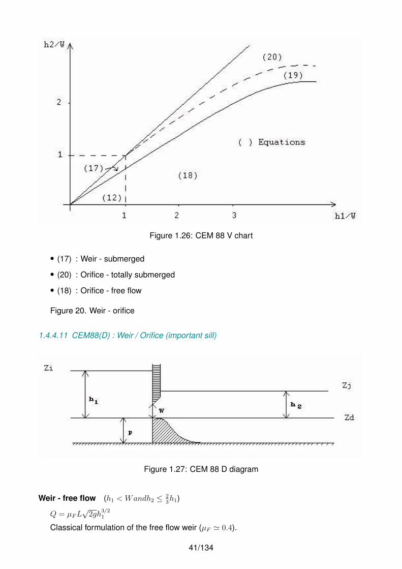
Figure 1.26: CEM 88 V chart
• (17) : Weir - submerged
• (20) : Orifice - totally submerged
• (18) : Orifice - free flow
Figure 20. Weir - orifice
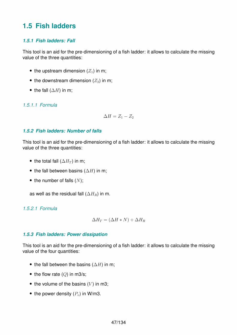
1.4.4.11 CEM88(D) : Weir / Orifice (important sill)
Figure 1.27: CEM 88 D diagram
Weir - free flow (h1 < Wandh2 ≤ 23h1)
Q = µFL√
2gh3/21
Classical formulation of the free flow weir (µF ' 0.4).
41/134

Weir - submerged flow (h1 < W and h2 ≥ 23h1)
Q = µSL√
2g(h1 − h2)1/2h2Classical formulation of the submerged weir.
The switch from submerged to free flow occurs for h2 = 23h1, we then have:
µS = 3√3
2µF for µF = 0.4⇒ µS = 1.04
An equivalent free flow coefficient can be calculated:
µF = Q
L√2gh
3/21
which makes it possible to evaluate the degree of flooding of the threshold by compar-ing it to the free coefficient µF introduces. Indeed, the master coefficient of the structureintroduced is that of the free weir. (µF close to 0.4).
Orifice - free flow (h1 ≥ W and h2 ≤ 23h1)
We take a formulation like:
Q = µL√
2g(h3/21 − (h1 −W )3/2
)This modeling applies well to large rectangular orifices.
Continuity to free surface operation is ensured when:h1W
= 1, we then have µ = µF .
Orifice - submerged flow There are two formulations depending on whether the orifice ispartially submerged or totally submerged.
Partially submerged flow (h1 ≥ W and 23h1 < h2 <
23h1 + W
3)
Q = µFL√
2g[3√3
2
((h1 − h2)1/2 h2
)− (h1 −W )3/2
]Totally submerged flow (h1 ≥ W and 2
3h1 + W
3< h2)
(Q = µ′L√
2g(h_1− h_2)Θ{1/2} [h2 − (h2 −W )]⇒ Q = µ′L√
2g(h_1− h_2)Θ{1/2}W )
Classical formulation of submerged orifices, with µ′ = µS.
Orifice weir operation is represented by the equations above and Figure 19. Regardlessof the type of flow under load, an equivalent free flow coefficient is calculated correspondingto the conventional free orifice formulation:
CF = QL√2gW (h1−0.5W )1/2
• (12) : Weir - free flow
• (15) : Orifice - partially submerged
• (13) : Weir - submerged
• (16) : Orifice - totally submerged
• (14) : Orifice - free flow
42/134

Figure 1.28: CEM 88 D chart
Figure 19. Weir - Orifice
1.4.4.12 Cunge 1980 formula
This stage discharge equation is based on the equations described by Cunge in his book 5,or in more detail in an article by Mahmood and Yevjevich 6. This law is a compilation of theclassical laws taking into account the different flow conditions: submerged, free flow, freesurface and in charge as well as the equations CEM88(D) : Weir / Orifice (important sill)and CEM88(D) : Weir / Orifice (low sill). However, contrary to these equations, it does notprovide any continuity between free surface and in charge flow conditions. This can lead todesign problems in the vicinity of this transition.
This law is suitable for a broad-crested rectangular weir, possibly in combination witha valve. The default discharge coefficient Cd = 1 corresponds to the following dischargecoefficients for the classical equations:
• Cd = 0.385 for the free flow weir](seuil_denoye.md).
• Cd = 1 for the submerged weir.
• Cd = 1 for the submerged gate.
• Cc = 0.611 for [the free flow gate with Cd calculated from Cc (See below).5Raynal, S., Courret, D., Chatellier, L., Larinier, M., David, L., 2012. Définition de prises d’eau ichty-
ocompatibles -Pertes de charge au passage des plans de grille inclinés ou orientés dans des configurationsichtyocompatibles et champs de vitesse à leur approche (POLE RA11.02). https://continuite-ecologique.fr/wp-content/uploads/2019/11/2012_014.pdf
6Raynal, S., Chatellier, L., Courret, D., Larinier, M., David, L., 2013. An experimental study on fish-friendlytrashracks–Part 2. Angled trashracks. Journal of Hydraulic Research 51, 67–75.
43/134

Free flow / submerged regime detection The flow regime is in free flow as long as thedownstream water level is below critical height:
(Z2 − Zdv) <2
3(Z1 − Zdv)
with Z1 upstream water elevation, Z2 downstream water elevation, et Zdv apron or sillelevation of the hydraulic structure.
Free flow / in charge flow detection The water level at the gate when the gate is open isconsidered here to be equal to:
• the critical height in the case of a free flow regime;
• the downstream water height in the case of a submerged regime.
The flow becomes in charge when the gate touches the surface of the water at this point.
In free flow, the flow is in charge when:
W ≤ 2
3(Z1 − Zdv)
In submerged flow, the condition becomes:
W ≤ Z2
Discharge equations The free flow gate equation uses a fixed contraction coefficient Ccwith:
Cd = Cc√1+CcW/ham
For all other flow regimes, used equations here are the following as they can be usedindependently:
Free surface In charge
Free flow Free flow weir](seuil_denoye.md) free flow gateSubmerged Submerged weir [Submerged gate
1.4.4.13 Free flow gate
Excerpt from Baume, J.-P., Belaud, G., Vion, P.-Y., 2013. Hydraulique pour le génie ru-ral, Formations de Master, Mastère Spécialisé, Ingénieur agronome. UMR G-EAU, Irstea,SupAgro Montpellier.
W is the gate opening, ham the upstream water level and L the date width. The dewa-tered valve equation is derived from Bernoulli’s load conservation relationship between theupstream side of the valve and the contracted section.
The height h2 corresponds to the contracted section and is equal to CcW where Cc is the
44/134

Figure 1.29: Free flow gate diagram
contraction coefficient. The free flow gate equation is often expressed as a function of a flowcoefficient in the form of:
Q = CdLW√
2g√ham
So we have the relationship between Cd and Cc :
Cd = Cc√1+CcW/ham
Numerous experiments were conducted to evaluate Cd, which varies little around 0.6. Asa first approximation, for a low W/ham (undershot gate, most frequent case), Cd is close toCc and can be chosen equal to 0.6.
Discharge coefficients Cd are given by abacuses, which can be found in specializedbooks if necessary. They range from 0.5 to 0.6 for a vertical gate, from 0.6 to 0.7 for aradial gate, up to 0.8 for a gate inclined with respect to the vertical.
1.4.4.14 Submerged gate
Figure 1.30: Submerged gate diagram
45/134

Excerpt from Baume, J.-P., Belaud, G., Vion, P.-Y., 2013. Hydraulique pour le génierural, Formations de Master, Mastère Spécialisé, Ingénieur agronome. UMR G-EAU, Irstea,SupAgro Montpellier.
Submerged gate equation Q = C ′dLW√
2g√ham − hav
Coefficient C ′d is around 0.8.
1.4.4.15 Villemonte 1947
The “Villemonte (1947)” equation uses the equation of the Free weir to which the flooding co-efficient proposed by Villemonte applies (see explanations below). This flooding coefficientis also used for the triangular and truncated triangular weir formulas.
Figure 1.31: Villemonte formula: submerged weir diagram
For a downstream water elevation higher than the crest elevation of the weir, the flow isflooded and a flooding coefficient is applied to the flow coefficient.
Villemonte proposes the following formula:
K =Qsubmerged
Qfree
=
[1−
(h2
h1
)n]0.385With:
• h1 the upstream water level above the crest of the weir
• h2 the downstream water level above the crest of the weir
• n the exponent in free flow relationships (rectangular=1.5, triangular=2.5, parabolic=2)
Villemonte, J.R., 1947. Submerged weir discharge studies. Engineering news record866, 54–57.
46/134
1.5 Fish ladders
1.5.1 Fish ladders: Fall
This tool is an aid for the pre-dimensioning of a fish ladder: it allows to calculate the missingvalue of the three quantities:
• the upstream dimension (Z1) in m;
• the downstream dimension (Z2) in m;
• the fall (∆H) in m;
1.5.1.1 Formula
∆H = Z1 − Z2
1.5.2 Fish ladders: Number of falls
This tool is an aid for the pre-dimensioning of a fish ladder: it allows to calculate the missingvalue of the three quantities:
• the total fall (∆HT ) in m;
• the fall between basins (∆H) in m;
• the number of falls (N );
as well as the residual fall (∆HR) in m.
1.5.2.1 Formula
∆HT = (∆H ∗N) + ∆HR
1.5.3 Fish ladders: Power dissipation
This tool is an aid for the pre-dimensioning of a fish ladder: it allows to calculate the missingvalue of the four quantities:
• the fall between the basins (∆H) in m;
• the flow rate (Q) in m3/s;
• the volume of the basins (V ) in m3;
• the power density (Pv) in W/m3.
47/134
The formula for calculating the power dissipation is then:
Pv =ρgQ∆H
V
with:
• ρ: the density of water;
• g: the acceleration of the Earth’s gravity = 9.81 m.s-2
1.5.4 Fish ladders: Dimensions
This tool is an aid for dimensioning the basins of a pass: it allows to calculate the missingvalue of the four quantities:
• the volume of water (V ) in m3;
• the mean draught (Ymean) in m;
• the length of the basin (L) in m;
• the width of the basin (B) in m.
The calculation is carried out by applying the formula:
V = Ymean × L×B
1.5.5 Cross walls
This tool, which is similar to the Parallel Structures tool, is an aid to the hydraulic pre-dimensioning of a fish pass: it is most often used for the dimensioning of notches, slots,orifices, etc. characterizing the walls of a pass as well as for the setting in altitude of thenotches, slots and apron of the upstream basin of a pass.
It allows to calculate the missing value of the 7 values characterizing the fall, the surfaceof the submerged orifice, the width of the slot, the load on the slot, the width of the notch,the load on the notch and the flow rate.
Mandatory data to be provided are the dimensions of the basins (width and length) andthe average draught in metres. These data associated with the fall between basins allow usto calculate the power dissipation.
Once the module is calculated, the tool proposes to create a basin pass from this crosswall by specifying the upstream water elevation, the number of falls in the pass and thedownstream water elevation.
1.5.5.1 Hydraulic structures that can be part of the cross wall
The tool allows you to place one or more structures in parallel among the following types ofstructures:
48/134

Figure 1.32: Submerged orifice diagram
Submerged orifice Excerpt from Larinier, M., Travade, F., Porcher, J.-P., Gosset, C., 1992.Fish passage: expertise and design of crossing structures. CSP. (page 94).
The submerged orifice equation is described on the submerged orifice formula page.
Submerged Slot Excerpt from Larinier, M., Travade, F., Porcher, J.-P., Gosset, C., 1992.Fish passage: expertise and design of crossing structures. CSP. (page 94).
The submerged slot equation is described on the sumberged slot formula page.
Notch Excerpt from Larinier, M., Travade, F., Porcher, J.-P., Gosset, C., 1992. Fish pas-sage: expertise and design of crossing structures. CSP. (page 94).
The equation used for the notch is that of Kindsvater-Carter and Villemonte.
1.5.6 Fish ladder
1.5.6.1 General presentation
This module calculates the water line of a fish ladder with successive basins. Two calculationpossibilities are offered: calculation of the inflow into the channel from the upstream anddownstream water levels, calculation of the upstream water level from the inflow into thechannel and the downstream water level.
The creation of a channel can be done from scratch or from a wall model created withthe Cross walls tool.
Input parameters are divided into two steps:
49/134

Figure 1.33: Schematic of the submerged slot
Figure 1.34: Notch diagram
• The hydraulic parameters which include the boundary conditions (water level upstreamand downstream of the fish ladder) and the inflow into the fish ladder.
• The parameters of the basins, which include the geometry of the basins and the pa-rameters of the hydraulic structures constituting the walls.
50/134

It is possible to vary one or two hydraulic parameters so as to obtain a series of resultsfor several boundary conditions or flows.
1.5.6.2 Input of the pass geometry
The geometry table has a line for each basin and a final line to describe the downstreamwall. For each basin, the parameters present are
• length of the basin (m)
• basin width (m)
• attraction flow (m3/s)
• Mid-basin invert rating (m)
• Upstream invert elevation (m)
To these are added the parameters of the structures of the upstream wall of each basin.
Modification of the pass structure The structure of the pass, i.e. the number of basinsor the number of structures in a wall can be changed using the toolbar at the top right of thetable:
Figure 1.35: Edit toolbar for the geometry of the pass
This bar is activated when you select:
• a basin (which includes its upstream wall) or the downstream wall by clicking on thefirst column of a row
• a structure by clicking on an uneditable cell of a structure in a wall
• all structures in a column of the table by clicking on the header of the column to beselected
It is also possible to expand an existing selection by pressing the Ctrl] key to add a newitem to the selection, or by pressing the [Shift] key to expand the selection between two rowsor two columns.
Depending on the elements selected in the table, the toolbar indicates whether the pro-posed actions will apply to the selected basins or structures.
The toolbar consists of the following buttons:
1. Number of basins or structures to be added or duplicated
2. Add n basins or n structures with n the number indicated on the first button.
51/134

3. Duplicate n basins or n structures with n the number indicated on the first button.
4. Delete selected basins or structures
5. 1. Move the selected pools (or structures) upwards (or to the left).
6. 1. Move the selected basins (or structures) downwards (or to the right).
Advanced modification of the pass geometry The selection of basins or structures givesaccess to a button “Modify values” which allows to modify a parameter among all the vari-ables of the selected cells in the geometry table.
For this variable to be modified, one can:
• define a fixed value;
• apply a delta;
• calculate an interpolation between the basin selected upstream and downstream.
The downstream wall The downstream wall, in addition to the laws of structures availableon the walls, allows the use of a “lift gate” in the form of two laws:
• Regulated notch (Villemonte 1957);
• Regulated submerged slot (Larinier 1992).
The lift gate is a structure where the crest of the weir is regulated to maintain a set-point waterfall between the last basin and the downstream water level. In addition to theconventional parameters of the flow laws, it includes:
• a DH setpoint waterfall (m)
• a minimum crest elevation minZDV (m);
• a maximum crest elevation maxZDV (m);
During the calculation, if the calculated crest elevation is less than minZDV (resp. greaterthan maxZDV ), the value is locked at minZDV (resp. maxZDV ) and a warning appears inthe calculation log.
1.5.6.3 Calculation results
The results are presented in the form of a summary table of hydraulic calculations for allbasins and walls. It contains all the data calculated by the modules Cross walls and Powerdissipation.
Two graphs are present:
• A profile along the channel with the apron elevation of the basins and the water eleva-tion in each basin.
52/134
• A general graph allowing the selection of any parameter from the result table in ab-scissa and ordinate.
If several results are available due to the variation of one or two hydraulic parametersof the pass, all calculated water lines are displayed in the long profile, and a drop-down listallows to select the result to be displayed in the generalist table and graph.
1.5.7 Pre-barrages
Pre-barrages are a type of basin pass used for crossing low obstacles. They are made up ofseveral walls or thresholds dividing the fall into several large basins in parallel and in series.
1.5.7.1 General presentation
This module calculates the flow distribution and the water line of the basins of a pre-barrage.Two calculation possibilities are offered: calculation of the channel flow into knowing theupstream and downstream water level, calculation of the upstream water level knowing thechannel flow and the downstream water level.
The input of the pre-barrage parameters is divided into two parts:
• The composition of the pre-barrage in basins and the walls connecting the basins, onthe first part of the screen.
• The input of the pre-barrage parameters: boundary conditions, basin parameters andwalls parameters, on the second part of the screen.
It is possible to vary any parameter in order to obtain a series of results.
The pre-barrage composition scheme can be displayed in full screen and exported toPNG image format.
1.5.7.2 Pre-barrage composition
At its creation, the pre-barrage consists of an upstream boundary condition, a basin, a down-stream boundary condition and walls joining these three elements.
The buttons “Add new basin” and “Add new wall” are used to add respectively a basin anda wall to the pre-barrage. When adding a wall, you are asked to which boundary conditionsor basins the wall is connected. When entering the connections to the walls, the user mustfollow the numbering of the basins, which necessarily respects an upstream-downstreamorder.
A toolbar allows to duplicate and delete a selected wall or basin and to change the orderof a basin.
1.5.7.3 Entering parameters of the pre-barrage elements
The entry of the parameters of the upstream or downstream boundary condition, of a basinor a wall is made by selecting the desired element in the diagram in the first part of thescreen.
53/134

The entry of the elements is then carried out as for any Cassiopée module. For the entryof walls, refer to the module [Parallel structures.
1.5.7.4 Launching the calculation
The calculate button is activated from the moment all the basins are connected by walls fromupstream to downstream of the pre-barrage and all the parameters have been entered.
1.5.7.5 Visualization of the results
After the calculation, the interface displays two tabs “Input” and “Results” that allow to navi-gate between the pre-barrage input and the calculation results.
If the calculation produces a series of results, a drop-down list allows you to choosewhich result to display for each parameter that has changed.
The first part of the screen shows a synoptic of the pre-barrage with the flows and fallsat the walls, the average power dissipated and the average depth at the basins, and theflow and water levels at the upstream and downstream boundary conditions. To view thenumerical results at basin level, the user must click on one of these items on the diagram.To view the numerical results at a wall, click on the corresponding wall on the diagram.
An “Export all results” button allows you to retrieve a table in Excel format containing theresults of boundary conditions, basins and walls for the whole calculation series.
1.6 Rock-ramp fishpasses
1.6.1 Rock-ramp fishpasses
The rock-ramp fishpass calculation module makes it possible to calculate the characteristicsof a rock-ramp pass made up of uniformly distributed blocks with equal transverse ax andlongitudinal ay spacings.
Figure 1.36: Schematic of a regular arrangement of rockfill and notations
54/134

Excerpt from Larinier et al., 20067
The tool allows you to calculate one of the following values:
• The width of the pass (m);
• The slope of the pass (m);
• The flow rate (m3/s);
• The depth h (m);
• The concentration of the blocks.
It requires the following values to be entered:
• The upstream bottom coordinate (m);
• The length of the pass (m);
• The background roughness (m);
• The width of the blocks D facing the flow (m);
• The useful height of the blocks k (m);
• The drag coefficient of a single block (1 for round, 2 for square).
1.6.2 Calculation of the flow rate of a rock-ramp pass
The calculation of the flow rate of a rock-ramp pass corresponds to the implementation ofthe algorithm and the equations present in Cassan et al. (2016)8.
1.6.2.1 General calculation principle
After Cassan et al., 20169
There are three possibilities:
• the submerged case when h ≥ 1.1× k
• the emergent case when h ≤ k
7Raynal, S., Courret, D., Chatellier, L., Larinier, M., David, L., 2012. Définition de prises d’eau ichty-ocompatibles -Pertes de charge au passage des plans de grille inclinés ou orientés dans des configurationsichtyocompatibles et champs de vitesse à leur approche (POLE RA11.02). https://continuite-ecologique.fr/wp-content/uploads/2019/11/2012_014.pdf
8Raynal, S., Courret, D., Chatellier, L., Larinier, M., David, L., 2012. Définition de prises d’eau ichty-ocompatibles -Pertes de charge au passage des plans de grille inclinés ou orientés dans des configurationsichtyocompatibles et champs de vitesse à leur approche (POLE RA11.02). https://continuite-ecologique.fr/wp-content/uploads/2019/11/2012_014.pdf
9Raynal, S., Courret, D., Chatellier, L., Larinier, M., David, L., 2012. Définition de prises d’eau ichty-ocompatibles -Pertes de charge au passage des plans de grille inclinés ou orientés dans des configurationsichtyocompatibles et champs de vitesse à leur approche (POLE RA11.02). https://continuite-ecologique.fr/wp-content/uploads/2019/11/2012_014.pdf
55/134

Figure 1.37: Organigramme de la méthode de calcul
• the quasi-emergent case when k < h < 1.1× k
In the quasi-emergent case, the calculation of the flow corresponds to a transition be-tween emergent and submerged case formulas:
Q = a×Qsubmerge + (1− a)×Qemergent
with a =h/k − 1
1.1− 1
1.6.2.2 Submerged case
The calculation is done by integrating the velocity profile in and above the macro-roughnesses.The calculated velocities are the temporal and spatial averages per plane parallel to the bot-tom.
In macro-roughnesses, velocities are obtained by double averaging the Navier-Stokesequations in uniform regime with a mixing length model for turbulence.
Above the macro-roughnesses, the classical turbulent boundary layer analysis is main-tained. The velocity profile is continuous at the top of the macro-roughnesses and is depen-dent on the boundary conditions set by the hydraulics:
56/134
• velocity at the bottom (without turbulence) in m/s:
u0 =√
2gSD(1− σC)/(CdC)
• total shear stress at the top of the roughnesses in m/s:
u∗ =√gS(h− k)
The average bed velocity is given by integrating the flows between and above the blocks:
u =Qinf +Qsup
h
with respectively Qinf and Qsup the unit flows for the part in the canopy and the part abovethe canopy.
Calculation of the unit flow rate Qinf in the canopy The flow in the canopy is obtainedby integrating the velocity profile (Eq. 9, Cassan et al., 2016):
Qinf =
∫ 1
0
u(z)dz
with
u(z) = u0
√β
(h
k− 1
)sinh(βz)
cosh(β)+ 1
with
β =√
(k/αt)(CdCk/D)/(1− σC)
with
Cd = Cxfh∗(h∗)
and αt obtained by solving the following equation:
αtu(1)− l0u∗ = 0
with
l0 = min (s, 0.15k)
with
s = D
(1√C− 1
)57/134
Calculation of the unit flow Qsup above the canopy
Qsup =
∫ h
k
u(z)dz
with (Eq. 12, Cassan et al., 2016)
u(z) =u∗κ
ln
(z − dz0
)with (Eq. 14, Cassan et al., 2016)
z0 = (k − d) exp
(−κuku∗
)and (Eq. 13, Cassan et al., 2016)
d = k − αtukκu∗
which gives
Qsup =u∗κ
((h− d)
(ln
(h− dz0
)− 1
)−(
(k − d)
(ln
(k − dz0
)− 1
)))
1.6.2.3 Emerging case
The calculation of the flow rate is done by successive iterations which consist in finding theflow rate value allowing to obtain the equality between the flow velocity V and the averagevelocity of the bed given by the equilibrium of the friction forces (bottom + drag) with gravity:
u0 =
√2gSD(1− σC)
CdfF (F )C(1 +N)
with
N =αCf
CdfF (F )Ch∗
with
α = 1− (ay/ax × C)
1.6.2.4 Formulas used
Bulk velocity V
V =Q
B × h
58/134

Average speed between blocks Vg From Eq. 1 Cassan et al (2016)10 and Eq. 1 Cassanet al (2014)11:
Vg =V
1−√
(ax/ay)C
Drag coefficient of a single block Cd0 Cd0 is the drag coefficient of a block consideringa single block infinitely high with F << 1 (Cassan et al, 201412).
Blockshape Cylinder
“Rounded face”shape
Square-basedparallelepiped “Flat face” shape
bloc_cylindre.png
bloc_face_arrondie.pngbloc_base_carree.png
Value ofCd0
1.0 1.2-1.3 2.0 2.2
When establishing the statistical formulae for the 2006 technical guide (Larinier et al. 2006[ˆ4]),the definition of the block shapes to be tested was based on the use of quarry blocks withneither completely round nor completely square faces. The so-called “rounded face” shapewas thus not completely cylindrical, but had a trapezoidal bottom face (seen in plan). Simi-larly, the “flat face” shape was not square in cross-section, but also had a trapezoidal bottomface. These differences in shape between the “rounded face” and a true cylinder on the onehand, and the “flat face” and a true parallelepiped with a square base on the other hand,result in slight differences between them in the shape coefficients Cd0.
Block shape coefficient Cassan et al. (2014)13, et Cassan et al. (2016)14 define σ as theratio between the block area in the x, y plane and D2. For the cylindrical form of the blocks,σ is equal to π/4 and for a square block, σ = 1.
10Raynal, S., Courret, D., Chatellier, L., Larinier, M., David, L., 2012. Définition de prises d’eau ichty-ocompatibles -Pertes de charge au passage des plans de grille inclinés ou orientés dans des configurationsichtyocompatibles et champs de vitesse à leur approche (POLE RA11.02). https://continuite-ecologique.fr/wp-content/uploads/2019/11/2012_014.pdf
11Raynal, S., Chatellier, L., Courret, D., Larinier, M., David, L., 2013. An experimental study on fish-friendlytrashracks–Part 2. Angled trashracks. Journal of Hydraulic Research 51, 67–75.
12Raynal, S., Chatellier, L., Courret, D., Larinier, M., David, L., 2013. An experimental study on fish-friendlytrashracks–Part 2. Angled trashracks. Journal of Hydraulic Research 51, 67–75.
13Raynal, S., Chatellier, L., Courret, D., Larinier, M., David, L., 2013. An experimental study on fish-friendlytrashracks–Part 2. Angled trashracks. Journal of Hydraulic Research 51, 67–75.
14Raynal, S., Courret, D., Chatellier, L., Larinier, M., David, L., 2012. Définition de prises d’eau ichty-ocompatibles -Pertes de charge au passage des plans de grille inclinés ou orientés dans des configurationsichtyocompatibles et champs de vitesse à leur approche (POLE RA11.02). https://continuite-ecologique.fr/wp-content/uploads/2019/11/2012_014.pdf
59/134

Ratio between the average speed downstream of a block and the maximum speed rThe values of () depends on the block shapes (Cassan et al., 201415 et Tran et al. 2016 16):
• round : rQ = 1.1
• “rounded face” shape : r = 1.2
• square-based parallelepiped : r = 1.5
• “flat face” shape : r = 1.6
Cassiopée implements a formula depending on Cd0:
r = 0.4Cd0 + 0.7
Froude FF =
Vg√gh
Froude-related drag coefficient correction function fF(F) If F < 1 (Eq. 19, Cassan etal., 201417):
fF (F ) = min
(r
1− F 2g
4
,1
F23
)2
otherwise fF (F ) = 1 because a torrential flow upstream of the blocks is theoreticallyimpossible because of the hydraulic jump caused by the downstream block.
Maximum speed umax According to equation 19 of Cassan et al, 201418 :
umax = Vg√fF (F )
Drag coefficient correction function linked to relative depth fh*(h*) The equation usedin Cassiopeia differs slightly from equation 20 of Cassan et al. 201419 and equation 6 of
15Raynal, S., Chatellier, L., Courret, D., Larinier, M., David, L., 2013. An experimental study on fish-friendlytrashracks–Part 2. Angled trashracks. Journal of Hydraulic Research 51, 67–75.
16Raynal, S., Courret, D., Chatellier, L., Larinier, M., David, L., 2013. An experimental study on fish-friendlytrashracks–Part 1. Inclined trashracks. Journal of Hydraulic Research 51, 56–66.
17Raynal, S., Chatellier, L., Courret, D., Larinier, M., David, L., 2013. An experimental study on fish-friendlytrashracks–Part 2. Angled trashracks. Journal of Hydraulic Research 51, 67–75.
18Raynal, S., Chatellier, L., Courret, D., Larinier, M., David, L., 2013. An experimental study on fish-friendlytrashracks–Part 2. Angled trashracks. Journal of Hydraulic Research 51, 67–75.
19Raynal, S., Chatellier, L., Courret, D., Larinier, M., David, L., 2013. An experimental study on fish-friendlytrashracks–Part 2. Angled trashracks. Journal of Hydraulic Research 51, 67–75.
60/134

Cassan et al. 201620. This formula is a fit to the experimental measurements on circularblocks used in Cassan et al. 201621:
fh∗(h∗) = (1 + 1/h2∗)
Coefficient of friction of the bed Cf If ks < 10−6m then we use Blasius’ formula
Cf = 0.3164/4 ∗Re−0.25
with
Re = u0 × h/ν
Else (Eq. 3, Cassan et al., 2016 d’après Rice et al., 1998)
Cf =2
(5.1log(h/ks) + 6)2
1.6.2.5 Notations
• α: ratio of the area affected by the bed friction to ax × ay
• αt: length scale of turbulence in the block layer (m)
• β: ratio between drag stress and turbulence stress
• κ: Von Karman constant = 0.41
• σ: ratio between the block area in the plane X,y et D2
• ax: cell width (perpendicular to the flow) (m)
• ay: length of a cell (parallel to the flow) (m)
• B: pass width (m)
• C: blocks concentration
• Cd: drag coefficient of a block under current flow conditions
• Cd0: drag coefficient of a block considering an infinitely high block with F � 1
• Cf ): bed friction coefficient
• d: displacement in the zero plane of the logarithmic profile (m)20Raynal, S., Courret, D., Chatellier, L., Larinier, M., David, L., 2012. Définition de prises d’eau ichty-
ocompatibles -Pertes de charge au passage des plans de grille inclinés ou orientés dans des configurationsichtyocompatibles et champs de vitesse à leur approche (POLE RA11.02). https://continuite-ecologique.fr/wp-content/uploads/2019/11/2012_014.pdf
21Raynal, S., Courret, D., Chatellier, L., Larinier, M., David, L., 2012. Définition de prises d’eau ichty-ocompatibles -Pertes de charge au passage des plans de grille inclinés ou orientés dans des configurationsichtyocompatibles et champs de vitesse à leur approche (POLE RA11.02). https://continuite-ecologique.fr/wp-content/uploads/2019/11/2012_014.pdf
61/134

• D: width of the block facing the flow (m)
• F : Froude number based on h and Vg
• g: acceleration of gravity = 9.81 m.s-2
• h: average depth (m)
• h∗: dimensionless depth (h/D)
• k: useful block height (m)
• ks: roughness height (m)
• l0: length scale of turbulence at the top of the blocks (m)
• N : ratio between bed friction and drag force
• Q: flow (m3/s)
• S: pass slope (m/m)
• u0: average bed speed (m/s)
• u∗: shear velocity (m/s)
• V : flow velocity (m/s)
• Vg: velocity between blocks (m/s)
• s: minimum distance between blocks (m)
• z: vertical position (m)
• z0: hydraulic roughness (m)
• z: dimensionless stand z = z/k
1.6.3 Compound rock-ramp fishpasses
This calculation module allows to calculate the flow passing through a rock-ramp pass called“complex” because it has an inclined apron or multiple aprons.
1.6.3.1 General characteristics
The parameters to be entered are the same as for the so-called “simple” macro-roughnesspass](macrorugo.md). Concerning the apron of the pass two choices are offered:
• Multiple aprons: it is possible to create, duplicate, delete, change the order of as manyaprons as necessary. For each apron, the parameters to be entered are: the width ofthe apron and the dimension of the apron upstream of the pass.
• The inclined apron: in addition to the width of the apron, the right and left sides of theapron must be entered upstream of the pass.
62/134

The calculated data are the same as for the so-called “simple” macro-roughness pass.The results display the different data for each apron and the graph allows you to view thisdata for each apron (transverse profile). In the event that at least one of the calculationparameters varies, the results are available individually via a drop-down list.
1.6.3.2 Inclined apron case
The calculation of an inclined apron pass consists in discretizing the pass into several hori-zontal aprons. The width of the created aprons is fixed at the distance between two blockswith an adjustment of the uppest apron to obtain the total width of the pass. It is possible toedit the created aprons by selecting “Multiple aprons” after performing a calculation with aninclined apron.
1.6.4 Blocks concentration
This module makes it possible to calculate the concentration of uniformly distributed blocksin a [rock-ramp fish pass.
It allows to calculate one of the following values:
• The width of the pass (m) ;
• The number of blocks ;
• The diameter of the blocks (m) ;
• The concentration of the blocks C.
1.6.4.1 Formula
Figure 1.38: Schematic of a regular arrangement of rockfill and notations
63/134

Excerpt from Larinier et al., 200622
The spacing between the blocks is then calculated with the following formula:
ax = ay =D√C
With :
• ax and ay respectively the longitudinal and lateral distances between the centres of theblocks (m);
• the width of the blocks facing the flow (m);
• the concentration of the blocks (-).
The number of blocks N for a pass of width B is then obtained with the equation:
N = B/ax
1.6.4.2 Harmonization
When calculating the number of blocks, if it is not an integer, upward and downward harmo-nized numbers of blocks are given along with corresponding concentration values.
Tolerance is of the order of a centimetre.
1.7 Baffle fishways
1.7.1 Baffle fishway (or baffle fishway) setup
This module allows to dimension a baffle fishway. Supported baffle fishway types are:
• plane baffles (Denil) fishway](theorie_plans.md);
• “Fatou” baffle fishway;
• [superactive baffles fishway;
• mixed / chevron baffles fishway.
See all the formulas used for baffle fishways.22Raynal, S., Courret, D., Chatellier, L., Larinier, M., David, L., 2012. Définition de prises d’eau ichty-
ocompatibles -Pertes de charge au passage des plans de grille inclinés ou orientés dans des configurationsichtyocompatibles et champs de vitesse à leur approche (POLE RA11.02). https://continuite-ecologique.fr/wp-content/uploads/2019/11/2012_014.pdf
64/134

1.7.1.1 Hydraulic setup
This tool allows to calculate one of the following values:
• flow through the pass (m3/s);
• upstream head (m);
• pass width (m) for plane and Fatou types.
Given the following mandatory parameters:
• pass type (Plane, Fatou, superactive, mixed);
• slope (m/m).
Parameter “Space between baffles (m)” is optional. When not given, its standard valueis calculated. When given, if its value deviates by more than 10% from standard value, anerror is generated.
1.7.1.2 Altimetric setup
Altimetric setup parameters (upstream water level and downstream water level) are optionaland allow to calculate:
• pass length in horizontal projection and following the slope
• number of baffles
• apron and spilling elevations, upstream and downstream
• rake height of upstream side walls
1.7.1.3 Generating a baffle fishway simulation module
Results of an altimetrically setup pass may be used to generate a baffle fishway simula-tion](simulation.md) module, using the ad hoc button. ## Baffle fishway (or baffle fishway)simulation
This module allows to calculate different hydraulic conditions on a baffle fishway with aknown geometry. This geometry may come from topographical measurements or from theresult of a baffle fishway setup.
Supported baffle fishway types are:
• plane baffles (Denil) fishway;
• “Fatou” baffle fishway;
• [superactive baffles fishway;
• mixed / chevron baffles fishway.
65/134

See all the formulas used for baffle fishways.
This tool allows to calculate one of the following values:
• flow through the pass (m3/s);
• upstream water elevation (m);
• upstream spilling elevation (m).
Given the following mandatory parameters:
• pass type (Plane, Fatou, superactive, mixed);
• slope (m/m).
• pass width (m);
• upstream spilling or apron elevation (m);
• downstream spilling or apron elevation (m).
1.7.2 Baffle fishways (or baffle fishways) calculation formulas
For calculation of:
• upstream head ha;
• water level in the pass h;
• flow Q;
• flow velocity V ;
• upstream apron elevation Zr1;
• minimal rake height of upstream side walls Zm
Refer to the formulas specific to each baffle fishway type:
• plane baffles (Denil) fishway](theorie_plans.md);
• “Fatou” baffle fishway;
• [superactive baffles fishway;
• mixed / chevron baffles fishway.
1.7.2.1 Upstream water elevation Z1
Z1 = Zd1 + ha
With Zd1 the spilling elevation of the first upstream baffle, ha the upstream head.
66/134
1.7.2.2 Pass length
Pass length along a water line parallel to the pass slope Lw equals
Lw = (Z1 − Z2)
√1 + S2
S
with Z1 and Z2 the upstream and downstream water elevations, S the slope.
Pass length along the slope LS must be a multiple of the length between two baffles Prounded to the greater integer:
LS = d(Lw − ε)/P e × P
With ε = 1 mm to leave a margin before adding an extra baffle.
Horizontal projection of the pass length Lh thus equals:
Lh =LS√
1 + S2
1.7.2.3 Number of baffles Nb
For plane and Fatou types:
Nb = LS/P + 1
For superactive and mixed types:
Nb = LS/P
1.7.2.4 Downstream apron Zr2 and spilling Zd2 elevations:
Zr2 = Zr1 −LS × S√
1 + S2
Zd2 = Zr2 + Zd1 − Zr1
1.7.3 Plane baffles (Denil) fishway
1.7.3.1 Geometrical characteristics
Excerpt from Larinier, 200223
23Raynal, S., Courret, D., Chatellier, L., Larinier, M., David, L., 2012. Définition de prises d’eau ichty-ocompatibles -Pertes de charge au passage des plans de grille inclinés ou orientés dans des configurationsichtyocompatibles et champs de vitesse à leur approche (POLE RA11.02). https://continuite-ecologique.fr/wp-content/uploads/2019/11/2012_014.pdf
67/134

Figure 1.39: Characteristics of a plane baffles (Denil) fishway
1.7.3.2 Hydraulic laws given by abacuses
Experiments conducted by Larinier, 200224 allowed to establish abacuses that link adimen-sional flow Q∗:
24Raynal, S., Courret, D., Chatellier, L., Larinier, M., David, L., 2012. Définition de prises d’eau ichty-ocompatibles -Pertes de charge au passage des plans de grille inclinés ou orientés dans des configurationsichtyocompatibles et champs de vitesse à leur approche (POLE RA11.02). https://continuite-ecologique.fr/wp-content/uploads/2019/11/2012_014.pdf
68/134

Q∗ =Q
√gL2,5
to upstream head ha and the average water level in the pass h :
Figure 1.40: Abacuses of a plane baffles (Denil) fishway for a slope of 10%
Abacuses of a plane baffles (Denil) fishway for a slope of 10% (Excerpt from Larinier,200225)
Figure 1.41: Abacuses of a plane baffles (Denil) fishway for a slope of 15%
Abacuses of a plane baffles (Denil) fishway for a slope of 15% (Excerpt from Larinier,200226)
Figure 1.42: Abacuses of a plane baffles (Denil) fishway for a slope of 20%
Abacuses of a plane baffles (Denil) fishway for a slope of 20% (Excerpt from Larinier,200227)
To run calculations for all slopes between 8% and 22%, polynomes coefficients of aba-cuses above are themelves adjusted in the form of slope S depending polynomes.
We thus have:
ha/L = a2(S)Q∗2 + a1(S)Q∗ + a0(S)
a2(S) = 315.110S2 − 115.164S + 6.85371
a1(S) = −184.043S2 + 59.7073S − 0.530737
a0(S) = 15.2115S2 − 5.22606S + 0.633654
And:
h/L = b2(S)Q∗2 + b1(S)Q∗ + b0
25Raynal, S., Courret, D., Chatellier, L., Larinier, M., David, L., 2012. Définition de prises d’eau ichty-ocompatibles -Pertes de charge au passage des plans de grille inclinés ou orientés dans des configurationsichtyocompatibles et champs de vitesse à leur approche (POLE RA11.02). https://continuite-ecologique.fr/wp-content/uploads/2019/11/2012_014.pdf
26Raynal, S., Courret, D., Chatellier, L., Larinier, M., David, L., 2012. Définition de prises d’eau ichty-ocompatibles -Pertes de charge au passage des plans de grille inclinés ou orientés dans des configurationsichtyocompatibles et champs de vitesse à leur approche (POLE RA11.02). https://continuite-ecologique.fr/wp-content/uploads/2019/11/2012_014.pdf
27Raynal, S., Courret, D., Chatellier, L., Larinier, M., David, L., 2012. Définition de prises d’eau ichty-ocompatibles -Pertes de charge au passage des plans de grille inclinés ou orientés dans des configurationsichtyocompatibles et champs de vitesse à leur approche (POLE RA11.02). https://continuite-ecologique.fr/wp-content/uploads/2019/11/2012_014.pdf
69/134

b2(S) = 347.368S2 − 130.698S + 8.14521
b1(S) = −139.382S2 + 47.2186S + 0.0547598
b0(S) = 16.7218S2 − 6.09624S + 0.834851
1.7.3.3 Calculation of ha, h and Q
We can then use those coefficients to calculate ha, h and Q∗:
ha = L(a2(Q
∗)2 + a1Q∗ + a0
)h = L
(b2(Q
∗)2 + b1Q∗ + b0
)Using the positive inverse function, depending on ha/L, we get:
Q∗ =−a1 +
√a21 − 4a2(a0 − ha/L)
2a2
And we finally have:
Q = Q∗√gL2,5
Calculation limitations of Q∗, ha/L and h/L are determined based on the extremities ofthe abacuses curves.
1.7.3.4 Flow velocity
Flow velocity V corresponds to the minimum flow speed given the flow section Aw at theperpendicular of the baffle :
V =Q
Aw
for plane baffles fishways using the notation of the schema above, we have:
Aw = B ×(h− C +D
2sin(45)
)Which gives with standard proportions:
Aw = L (0.583h− 0.146L)
1.7.3.5 Upstream apron elevation Zr1
Zr1 = Zd1 −D sin(45 + arctan(S))
70/134

1.7.3.6 Minimal rake height of upstream side walls Zm
Zm = Zr1 +−Hmin sin(45 + arctan(S))
1.7.4 “Fatou” baffle fiwhway
1.7.4.1 Geometrical characteristics
Figure 1.43: Characteristics of a Fatou baffle fishway
Excerpt fromLarinier, 200228
28Raynal, S., Courret, D., Chatellier, L., Larinier, M., David, L., 2012. Définition de prises d’eau ichty-ocompatibles -Pertes de charge au passage des plans de grille inclinés ou orientés dans des configurationsichtyocompatibles et champs de vitesse à leur approche (POLE RA11.02). https://continuite-ecologique.fr/wp-content/uploads/2019/11/2012_014.pdf
71/134

1.7.4.2 Hydraulic laws given by abacuses
Experiments conducted by Larinier, 200229 allowed to establish abacuses that link adimen-sional flow Q∗:
Q∗ =Q
√gL2,5
to upstream head ha and the average water level in the pass h :
Figure 1.44: Abacuses of a Fatou baffle fishway for a slope of 10%
Abacuses of a Fatou baffle fishway for a slope of 10% (Excerpt fromLarinier, 200230)
Figure 1.45: Abacuses of a Fatou baffle fishway for a slope of 15%
Abacuses of a Fatou baffle fishway for a slope of 15% (Excerpt fromLarinier, 200231)
Figure 1.46: Abacuses of a Fatou baffle fishway for a slope of 20%
Abacuses of a Fatou baffle fishway for a slope of 20% (Excerpt fromLarinier, 200232)
To run calculations for all slopes between 8% and 22%, polynomes coefficients of aba-cuses above are themelves adjusted in the form of slope S depending polynomes.
We thus have:
ha/L = a2(S)Q∗2 + a1(S)Q∗ + a0(S)
a2(S) = −783.592S2 + 269.991S − 25.2637
a1(S) = 302.623S2 − 106.203S + 13.2957
a0(S) = 15.8096S2 − 5.19282S + 0.465827
29Raynal, S., Courret, D., Chatellier, L., Larinier, M., David, L., 2012. Définition de prises d’eau ichty-ocompatibles -Pertes de charge au passage des plans de grille inclinés ou orientés dans des configurationsichtyocompatibles et champs de vitesse à leur approche (POLE RA11.02). https://continuite-ecologique.fr/wp-content/uploads/2019/11/2012_014.pdf
30Raynal, S., Courret, D., Chatellier, L., Larinier, M., David, L., 2012. Définition de prises d’eau ichty-ocompatibles -Pertes de charge au passage des plans de grille inclinés ou orientés dans des configurationsichtyocompatibles et champs de vitesse à leur approche (POLE RA11.02). https://continuite-ecologique.fr/wp-content/uploads/2019/11/2012_014.pdf
31Raynal, S., Courret, D., Chatellier, L., Larinier, M., David, L., 2012. Définition de prises d’eau ichty-ocompatibles -Pertes de charge au passage des plans de grille inclinés ou orientés dans des configurationsichtyocompatibles et champs de vitesse à leur approche (POLE RA11.02). https://continuite-ecologique.fr/wp-content/uploads/2019/11/2012_014.pdf
32Raynal, S., Courret, D., Chatellier, L., Larinier, M., David, L., 2012. Définition de prises d’eau ichty-ocompatibles -Pertes de charge au passage des plans de grille inclinés ou orientés dans des configurationsichtyocompatibles et champs de vitesse à leur approche (POLE RA11.02). https://continuite-ecologique.fr/wp-content/uploads/2019/11/2012_014.pdf
72/134

And:
h/L = b2(S)Q∗2 + b1(S)Q∗ + b0
b2(S) = −73.4829S2 + 54.6733S − 14.0622
b1(S) = 42.4113S2 − 24.4941S + 8.84146
b0(S) = −3.56494S2 + 0.450262S + 0.0407576
1.7.4.3 Calculation of ha, h and Q
We can then use those coefficients to calculate ha, h and Q∗:
ha = L(a2(Q
∗)2 + a1Q∗ + a0
)h = L
(b2(Q
∗)2 + b1Q∗ + b0
)Using the positive inverse function, depending on ha/L, we get:
Q∗ =−a1 +
√a21 − 4a2(a0 − ha/L)
2a2
And we finally have:
Q = Q∗√gL2,5
Calculation limitations of Q∗, ha/L and h/L are determined based on the extremities ofthe abacuses curves.
1.7.4.4 Flow velocity
Flow velocity V corresponds to the minimum flow speed given the flow section Aw at theperpendicular of the baffle :
V =Q
Aw
for Fatou baffle fishways using the notation of the schema above, we have:
Aw = B × h
Which gives with standard proportions:
Aw = 0.6hL
73/134

1.7.4.5 Upstream apron elevation Zr1
Zr1 = Zd1 +0.3S − 0.2√
1 + S2
1.7.4.6 Minimal rake height of upstream side walls Zm
Zm = Zr1 +4L
3√
1 + S2
1.7.5 Superactive baffles fishway
Figure 1.47: Characteristics of a superactive baffles fishway
Excerpt from Larinier, 200233
1.7.5.1 Hydraulic laws given by abacuses
Experiments conducted by Larinier, 200234 allowed to establish abacuses that link adimen-sional flow q∗ :
33Raynal, S., Courret, D., Chatellier, L., Larinier, M., David, L., 2012. Définition de prises d’eau ichty-ocompatibles -Pertes de charge au passage des plans de grille inclinés ou orientés dans des configurationsichtyocompatibles et champs de vitesse à leur approche (POLE RA11.02). https://continuite-ecologique.fr/wp-content/uploads/2019/11/2012_014.pdf
34Raynal, S., Courret, D., Chatellier, L., Larinier, M., David, L., 2012. Définition de prises d’eau ichty-ocompatibles -Pertes de charge au passage des plans de grille inclinés ou orientés dans des configurations
74/134

q∗ =Q/L√2ga1,5
to upstream head ha and the average water level in the pass h :
Figure 1.48: Abacuses of a superactive baffles fishway for a slope of 10%
Abacuses of a superactive baffles fishway for a slope of 10% (Excerpt from Larinier,200235)
Figure 1.49: Abacuses of a superactive baffles fishway for a slope of 15%
Abacuses of a superactive baffles fishway for a slope of 15% (Excerpt from Larinier,200236)
To run calculations for all slopes between 8% and 22%, polynomes coefficients of aba-cuses above are themelves adjusted in the form of slope S depending polynomes.
We thus have:
ha/a = a2(S)q∗2 + a1(S)q∗ + a0(S)
a2(S) = −0.354624S − 0.0153156
a1(S) = 0.514953S + 1.25460
a0(S) = −2.22434S + 0.596682
And:
h/a = b2(S)q∗2 + b1(S)q∗ + b0
b2(S) = −0.559218S + 0.000504060
b1(S) = 1.15807S + 1.07554
b0(S) = −2.62712S + 0.601348
ichtyocompatibles et champs de vitesse à leur approche (POLE RA11.02). https://continuite-ecologique.fr/wp-content/uploads/2019/11/2012_014.pdf
35Raynal, S., Courret, D., Chatellier, L., Larinier, M., David, L., 2012. Définition de prises d’eau ichty-ocompatibles -Pertes de charge au passage des plans de grille inclinés ou orientés dans des configurationsichtyocompatibles et champs de vitesse à leur approche (POLE RA11.02). https://continuite-ecologique.fr/wp-content/uploads/2019/11/2012_014.pdf
36Raynal, S., Courret, D., Chatellier, L., Larinier, M., David, L., 2012. Définition de prises d’eau ichty-ocompatibles -Pertes de charge au passage des plans de grille inclinés ou orientés dans des configurationsichtyocompatibles et champs de vitesse à leur approche (POLE RA11.02). https://continuite-ecologique.fr/wp-content/uploads/2019/11/2012_014.pdf
75/134

1.7.5.2 Calculation of ha, h and Q
We can then use those coefficients to calculate ha, h and q∗:
ha = a(a2(q
∗)2 + a1q∗ + a0
)h = a
(b2(q
∗)2 + b1q∗ + b0
)Using the positive inverse function, depending on ha/L, we get:
q∗ =−a1 +
√a21 − 4a2(a0 − ha/a)
2a2
And we finally have:
Q = Lq∗√ga1,5
Calculation limitations of q∗, ha/a and h/a are determined based on the extremities of theabacuses curves.
1.7.5.3 Flow velocity
Flow velocity V corresponds to the minimum flow speed given the flow section Aw at theperpendicular of the baffle :
V =Q
Aw
for superactive baffles fishways using the notation of the schema above, we have:
Aw = h× L
1.7.5.4 Upstream apron elevation Zr1
Zr1 = Zd1 +2.6aS − a√
1 + S2
1.7.6 Mixed / chevron baffles fishway
Excerpt from Larinier, 200237
37Raynal, S., Courret, D., Chatellier, L., Larinier, M., David, L., 2012. Définition de prises d’eau ichty-ocompatibles -Pertes de charge au passage des plans de grille inclinés ou orientés dans des configurationsichtyocompatibles et champs de vitesse à leur approche (POLE RA11.02). https://continuite-ecologique.fr/wp-content/uploads/2019/11/2012_014.pdf
76/134

Figure 1.50: Characteristics of a mixed / chevron baffles fishway
1.7.6.1 Hydraulic laws given by abacuses
Experiments conducted by Larinier, 200238 allowed to establish abacuses that link adimen-sional flow q∗ :
38Raynal, S., Courret, D., Chatellier, L., Larinier, M., David, L., 2012. Définition de prises d’eau ichty-ocompatibles -Pertes de charge au passage des plans de grille inclinés ou orientés dans des configurationsichtyocompatibles et champs de vitesse à leur approche (POLE RA11.02). https://continuite-ecologique.fr/wp-content/uploads/2019/11/2012_014.pdf
77/134

q∗ =Q/L√2ga1,5
to upstream head ha and the average water level in the pass h :
Figure 1.51: Abacuses of a mixed / chevron baffles fishway for a slope of 10%
Abacuses of a mixed / chevron baffles fishway for a slope of 10% (Excerpt from Larinier,200239)
Figure 1.52: Abacuses of a mixed / chevron baffles fishway for a slope of 16%
Abacuses of a mixed / chevron baffles fishway for a slope of 15% (Excerpt from Larinier,200240)
To run calculations for all slopes between 8% and 22%, polynomes coefficients of aba-cuses above are themelves adjusted in the form of slope S depending polynomes.
We thus have:
ha/a = a2(S)q∗2 + a1(S)q∗ + a0(S)
a2(S) = 0.188324S − 0.0427461
a1(S) = −2.47998S + 1.25363
a0(S) = 5.02138S + 0.709434
And:
h/a = b2(S)q∗2 + b1(S)q∗ + b0
b2(S) = −0.0733832S − 0.00839864
b1(S) = 0.176261S + 0.661656
b0(S) = −4.97686S + 1.30546
39Raynal, S., Courret, D., Chatellier, L., Larinier, M., David, L., 2012. Définition de prises d’eau ichty-ocompatibles -Pertes de charge au passage des plans de grille inclinés ou orientés dans des configurationsichtyocompatibles et champs de vitesse à leur approche (POLE RA11.02). https://continuite-ecologique.fr/wp-content/uploads/2019/11/2012_014.pdf
40Raynal, S., Courret, D., Chatellier, L., Larinier, M., David, L., 2012. Définition de prises d’eau ichty-ocompatibles -Pertes de charge au passage des plans de grille inclinés ou orientés dans des configurationsichtyocompatibles et champs de vitesse à leur approche (POLE RA11.02). https://continuite-ecologique.fr/wp-content/uploads/2019/11/2012_014.pdf
78/134

1.7.6.2 Calculation of ha, h and Q
We can then use those coefficients to calculate ha, h and q∗:
ha = a(a2(q
∗)2 + a1q∗ + a0
)h = a
(b2(q
∗)2 + b1q∗ + b0
)Using the positive inverse function, depending on ha/L, we get:
q∗ =−a1 +
√a21 − 4a2(a0 − ha/a)
2a2
And we finally have:
Q = Lq∗√ga1,5
Calculation limitations of q∗, ha/a and h/a are determined based on the extremities of theabacuses curves.
1.7.6.3 Flow velocity
Flow velocity V corresponds to the minimum flow speed given the flow section Aw at theperpendicular of the baffle :
V =Q
Aw
for mixed / chevron baffles fishways using the notation of the schema above, we have:
Aw = h× L
1.7.6.4 Upstream apron elevation Zr1
Zr1 = Zd1 +3aS − a√
1 + S2
1.8 Crossability verification
1.8.1 Crossability verification
This module allows to verify the capacity of different fish species to cross the following typesof fish passes:
• fish ladders](pab.md)
• baffle fishways
79/134
• rock-ramp fishpasses
1.8.1.1 Principle
For each pass type, several crossability criteria are checked, expressed as threshold values(ex: minimal basin depth, for a fish ladder).
Exceeding the threshold value of a criterion leads to an explicit error mentioning thequantity concerned and the threshold value, and results in the pass not being crossable.
Some criteria such as maximal dissipated power have both an alert value (crossability ispossible but not guaranteed) and a limit value (crossing the pass is impossible).
For a given pass, one can check at once the crossing capabilities of several species, overmultiple modalities (variation of one or more parameters in the pass).
1.8.1.2 Predefined species
[Several common species groups are predefined: default values are associated to crossabil-ity criteria.
Default values for some of those criteria might be missing for a species group, when thelatter is considered unabled to cross the pass type the criterion is related to.
1.8.1.3 Custom species
The Fish species characteristics module allows to define custom values for allcriteria, before running a pass verification.
If a criterion is applicable to the pass that is being checked, but no value was given, anerror will be triggered when running the verification, leading to the pass being not crossable.
1.8.2 Crossability verification: Fish ladders
When verifying a fish ladder, basins and walls are sequentially tested, as well as everydevice of each wall. If at least one basin is not crossable, then the pass is not crossable.
Criteria differ depending on the jet type generated by the device being verified. If a wallhas several devices, it will be considered crossable if at least one device is crossable.
Orifices are considered uncrossable.
For certain species, values of certain criteria are not precisely known or are subject toslight changes depending on future feedback.
1.8.2.1 Criteria
Diving jet support Some species do not support diving jets. For such species, eachdevice leading to a diving jet is marked as not crossable.
Maximum fall, in m Basin fall must be lower than maximum fall.
80/134

Minimum slot width, in m (surface jet only) Slot width must be greater than minimumwidth.
Minimum orifice surface, in m² Orifice surface must be greater than minimum slot width(above), squared.
Minimum head on weir, in m Head on weir must be greater than minimum head.
Minimum basin depth, in m Basin depth must be greater than minimum depth. For divingjets, depth must be greater than twice the basin fall.
Minimum basin length, in m Basin length must be greater than minimum length.
Recommanded maximum dissipated power and limit maximum dissipated power, inW/m³ Maximal dissipated power in the basin must be lower than limit maximum dissipatedpower. If it is greater than recommanded maximum dissipated power, a warning is thrown.
Important: maximum dissipated power verification is disabled in the current Cassiopéeversion.
1.8.2.2 Criteria values for predefined species groups
From “Informations sur la Continuité Écologique - ICE, Onema 2014”, and et OFB com. pers.
Table 1.6: List of predefined values for crossing criteria of a fish ladder
ICE group Species
Minimumhead on weir(m)
Recommandedmaximumdissipatedpower (W/m³)
Limitmaximumdissipatedpower (W/m³)
1 Atlanticsalmon(Salmosalar)Sea orriver trout[50-100](Salmo trutta)
0.3 200 250
2 Mules (Chelonlabrosus, Lizaramada)
0.2 200 250
3a Gread shad(Alosa alosa)
0.4 150 200
3b Shad (Alosafallax fallax)
0.4 150 200
3c Sea lamprey(Petromyzonmarinus)
0.15 200 250
81/134
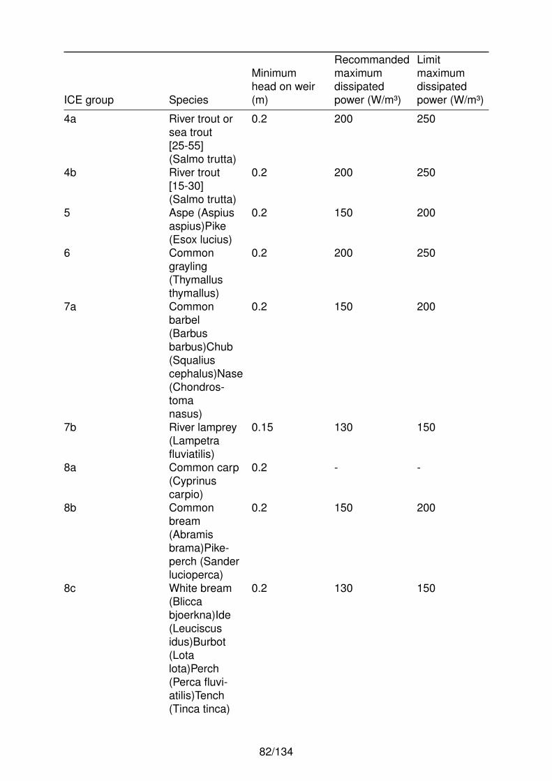
ICE group Species
Minimumhead on weir(m)
Recommandedmaximumdissipatedpower (W/m³)
Limitmaximumdissipatedpower (W/m³)
4a River trout orsea trout[25-55](Salmo trutta)
0.2 200 250
4b River trout[15-30](Salmo trutta)
0.2 200 250
5 Aspe (Aspiusaspius)Pike(Esox lucius)
0.2 150 200
6 Commongrayling(Thymallusthymallus)
0.2 200 250
7a Commonbarbel(Barbusbarbus)Chub(Squaliuscephalus)Nase(Chondros-tomanasus)
0.2 150 200
7b River lamprey(Lampetrafluviatilis)
0.15 130 150
8a Common carp(Cyprinuscarpio)
0.2 - -
8b Commonbream(Abramisbrama)Pike-perch (Sanderlucioperca)
0.2 150 200
8c White bream(Bliccabjoerkna)Ide(Leuciscusidus)Burbot(Lotalota)Perch(Perca fluvi-atilis)Tench(Tinca tinca)
0.2 130 150
82/134

ICE group Species
Minimumhead on weir(m)
Recommandedmaximumdissipatedpower (W/m³)
Limitmaximumdissipatedpower (W/m³)
8d Commondace(Leuciscus spbut Idus)
0.2 150 200
9a Bleak(Alburnusalbur-nus)Sprirlin(Alburnoidesbipuncta-tus)Mediterraneanbarbel(Barbusmeridion-alis)Souffia(Telestessouf-fia)Cruciancarp(Carassiuscaras-sius)Prussiancarp(Carassiusgibelio)Roach(Rutilus ru-tilus)Commonrudd(Scardiniuserythrophthalmus)South-westeuropeannase (Para-chondrostomatoxostoma)
0.2 130 150
83/134
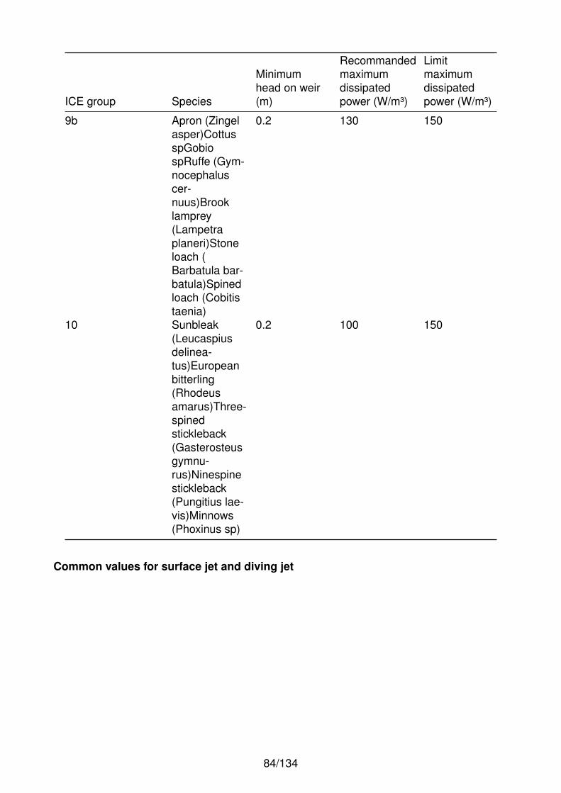
ICE group Species
Minimumhead on weir(m)
Recommandedmaximumdissipatedpower (W/m³)
Limitmaximumdissipatedpower (W/m³)
9b Apron (Zingelasper)CottusspGobiospRuffe (Gym-nocephaluscer-nuus)Brooklamprey(Lampetraplaneri)Stoneloach (Barbatula bar-batula)Spinedloach (Cobitistaenia)
0.2 130 150
10 Sunbleak(Leucaspiusdelinea-tus)Europeanbitterling(Rhodeusamarus)Three-spinedstickleback(Gasterosteusgymnu-rus)Ninespinestickleback(Pungitius lae-vis)Minnows(Phoxinus sp)
0.2 100 150
Common values for surface jet and diving jet
84/134
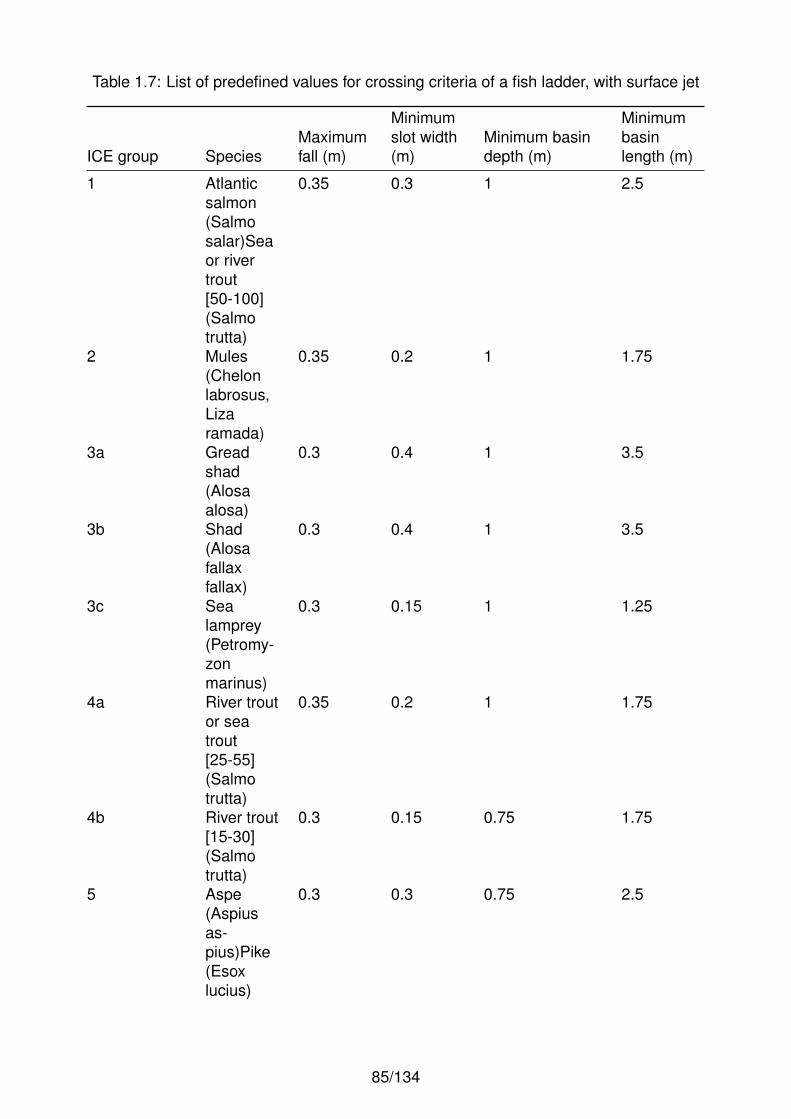
Table 1.7: List of predefined values for crossing criteria of a fish ladder, with surface jet
ICE group SpeciesMaximumfall (m)
Minimumslot width(m)
Minimum basindepth (m)
Minimumbasinlength (m)
1 Atlanticsalmon(Salmosalar)Seaor rivertrout[50-100](Salmotrutta)
0.35 0.3 1 2.5
2 Mules(Chelonlabrosus,Lizaramada)
0.35 0.2 1 1.75
3a Greadshad(Alosaalosa)
0.3 0.4 1 3.5
3b Shad(Alosafallaxfallax)
0.3 0.4 1 3.5
3c Sealamprey(Petromy-zonmarinus)
0.3 0.15 1 1.25
4a River troutor seatrout[25-55](Salmotrutta)
0.35 0.2 1 1.75
4b River trout[15-30](Salmotrutta)
0.3 0.15 0.75 1.75
5 Aspe(Aspiusas-pius)Pike(Esoxlucius)
0.3 0.3 0.75 2.5
85/134
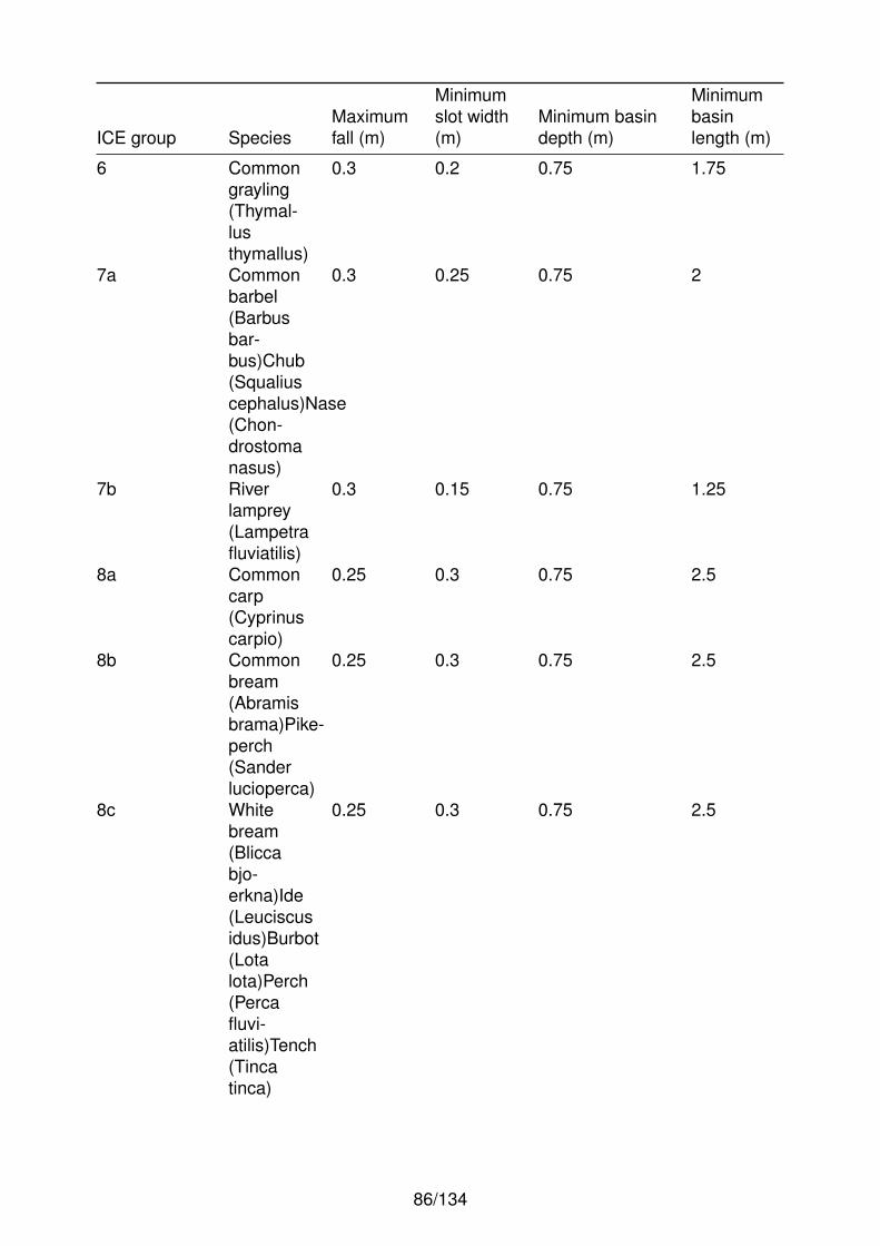
ICE group SpeciesMaximumfall (m)
Minimumslot width(m)
Minimum basindepth (m)
Minimumbasinlength (m)
6 Commongrayling(Thymal-lusthymallus)
0.3 0.2 0.75 1.75
7a Commonbarbel(Barbusbar-bus)Chub(Squaliuscephalus)Nase(Chon-drostomanasus)
0.3 0.25 0.75 2
7b Riverlamprey(Lampetrafluviatilis)
0.3 0.15 0.75 1.25
8a Commoncarp(Cyprinuscarpio)
0.25 0.3 0.75 2.5
8b Commonbream(Abramisbrama)Pike-perch(Sanderlucioperca)
0.25 0.3 0.75 2.5
8c Whitebream(Bliccabjo-erkna)Ide(Leuciscusidus)Burbot(Lotalota)Perch(Percafluvi-atilis)Tench(Tincatinca)
0.25 0.3 0.75 2.5
86/134
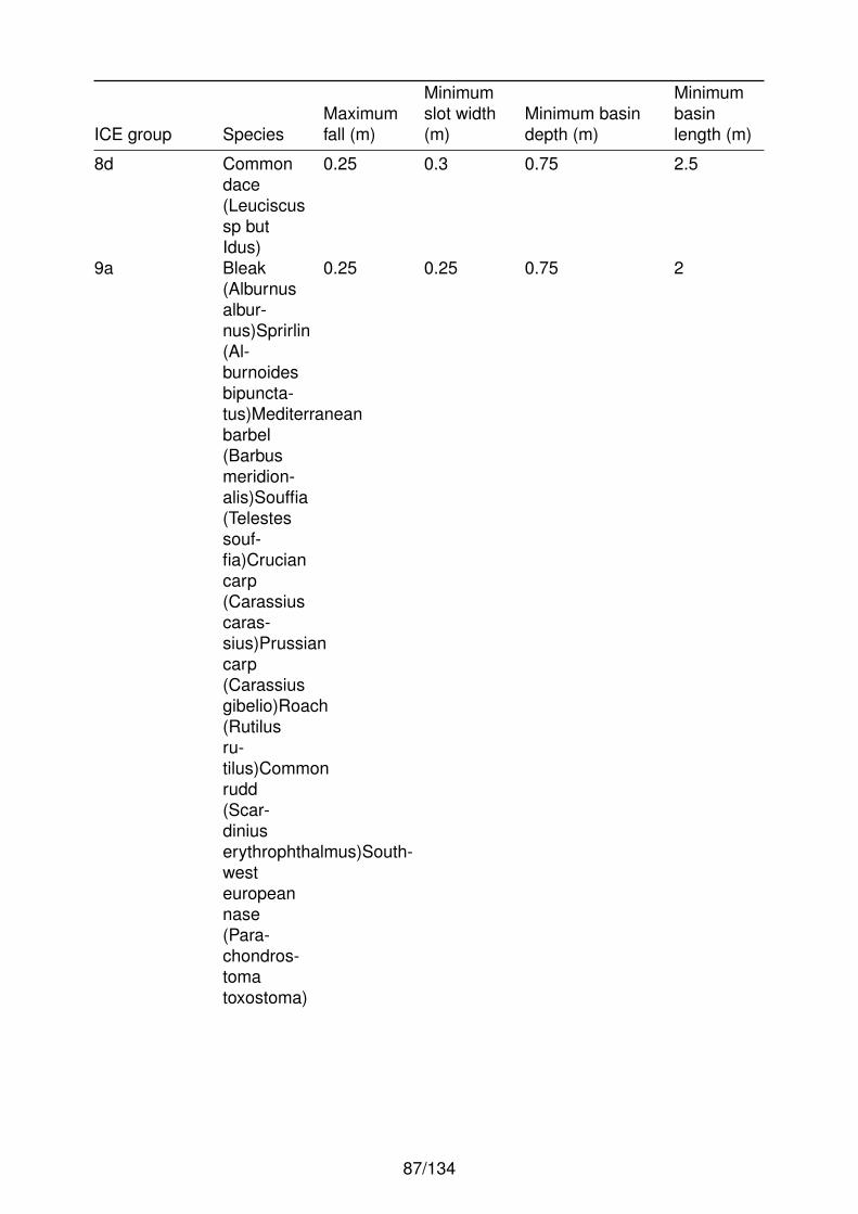
ICE group SpeciesMaximumfall (m)
Minimumslot width(m)
Minimum basindepth (m)
Minimumbasinlength (m)
8d Commondace(Leuciscussp butIdus)
0.25 0.3 0.75 2.5
9a Bleak(Alburnusalbur-nus)Sprirlin(Al-burnoidesbipuncta-tus)Mediterraneanbarbel(Barbusmeridion-alis)Souffia(Telestessouf-fia)Cruciancarp(Carassiuscaras-sius)Prussiancarp(Carassiusgibelio)Roach(Rutilusru-tilus)Commonrudd(Scar-diniuserythrophthalmus)South-westeuropeannase(Para-chondros-tomatoxostoma)
0.25 0.25 0.75 2
87/134

ICE group SpeciesMaximumfall (m)
Minimumslot width(m)
Minimum basindepth (m)
Minimumbasinlength (m)
9b Apron(Zingel as-per)CottusspGobiospRuffe(Gymno-cephaluscer-nuus)Brooklamprey(Lampetraplaneri)Stoneloach (Barbatulabarbat-ula)Spinedloach(Cobitistaenia)
0.2 0.15 0.5 1.25
10 Sunbleak(Leu-caspiusdelinea-tus)Europeanbitterling(Rhodeusamarus)Three-spinedstickle-back(Gasteros-teusgymnu-rus)Ninespinestickle-back(Pungitiuslae-vis)Minnows(Phoxinussp)
0.2 0.15 0.5 1.25
Surface jet
88/134
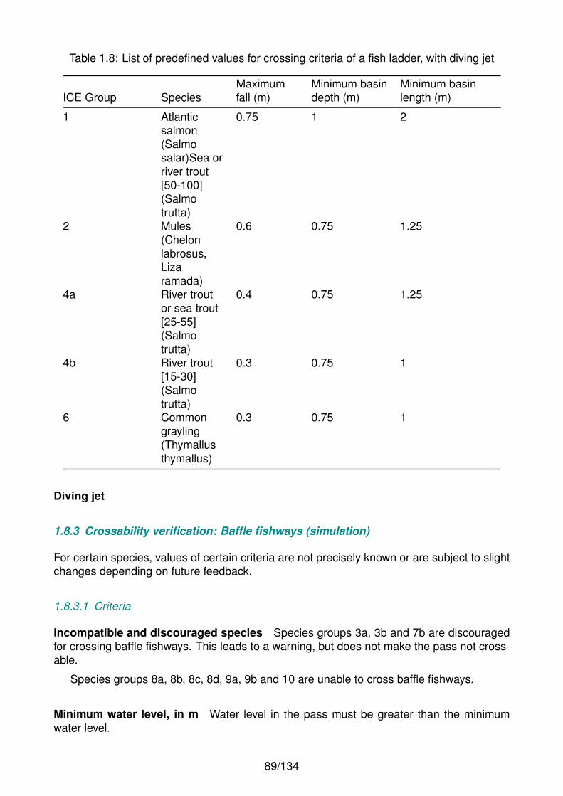
Table 1.8: List of predefined values for crossing criteria of a fish ladder, with diving jet
ICE Group SpeciesMaximumfall (m)
Minimum basindepth (m)
Minimum basinlength (m)
1 Atlanticsalmon(Salmosalar)Sea orriver trout[50-100](Salmotrutta)
0.75 1 2
2 Mules(Chelonlabrosus,Lizaramada)
0.6 0.75 1.25
4a River troutor sea trout[25-55](Salmotrutta)
0.4 0.75 1.25
4b River trout[15-30](Salmotrutta)
0.3 0.75 1
6 Commongrayling(Thymallusthymallus)
0.3 0.75 1
Diving jet
1.8.3 Crossability verification: Baffle fishways (simulation)
For certain species, values of certain criteria are not precisely known or are subject to slightchanges depending on future feedback.
1.8.3.1 Criteria
Incompatible and discouraged species Species groups 3a, 3b and 7b are discouragedfor crossing baffle fishways. This leads to a warning, but does not make the pass not cross-able.
Species groups 8a, 8b, 8c, 8d, 9a, 9b and 10 are unable to cross baffle fishways.
Minimum water level, in m Water level in the pass must be greater than the minimumwater level.
89/134
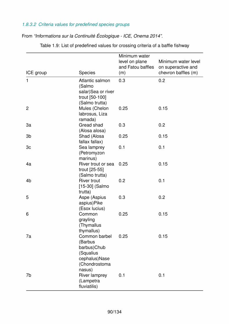
1.8.3.2 Criteria values for predefined species groups
From “Informations sur la Continuité Écologique - ICE, Onema 2014”.
Table 1.9: List of predefined values for crossing criteria of a baffle fishway
ICE group Species
Minimum waterlevel on planeand Fatou baffles(m)
Minimum water levelon superactive andchevron baffles (m)
1 Atlantic salmon(Salmosalar)Sea or rivertrout [50-100](Salmo trutta)
0.3 0.2
2 Mules (Chelonlabrosus, Lizaramada)
0.25 0.15
3a Gread shad(Alosa alosa)
0.3 0.2
3b Shad (Alosafallax fallax)
0.25 0.15
3c Sea lamprey(Petromyzonmarinus)
0.1 0.1
4a River trout or seatrout [25-55](Salmo trutta)
0.25 0.15
4b River trout[15-30] (Salmotrutta)
0.2 0.1
5 Aspe (Aspiusaspius)Pike(Esox lucius)
0.3 0.2
6 Commongrayling(Thymallusthymallus)
0.25 0.15
7a Common barbel(Barbusbarbus)Chub(Squaliuscephalus)Nase(Chondrostomanasus)
0.25 0.15
7b River lamprey(Lampetrafluviatilis)
0.1 0.1
90/134
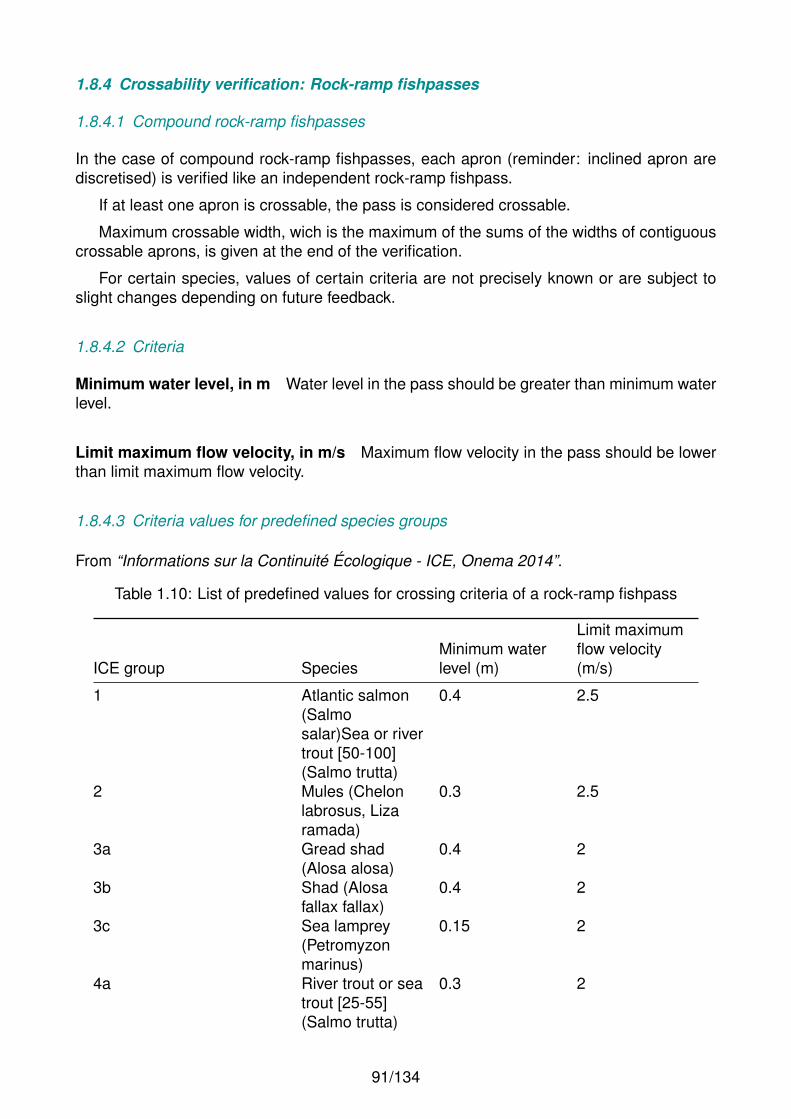
1.8.4 Crossability verification: Rock-ramp fishpasses
1.8.4.1 Compound rock-ramp fishpasses
In the case of compound rock-ramp fishpasses, each apron (reminder: inclined apron arediscretised) is verified like an independent rock-ramp fishpass.
If at least one apron is crossable, the pass is considered crossable.
Maximum crossable width, wich is the maximum of the sums of the widths of contiguouscrossable aprons, is given at the end of the verification.
For certain species, values of certain criteria are not precisely known or are subject toslight changes depending on future feedback.
1.8.4.2 Criteria
Minimum water level, in m Water level in the pass should be greater than minimum waterlevel.
Limit maximum flow velocity, in m/s Maximum flow velocity in the pass should be lowerthan limit maximum flow velocity.
1.8.4.3 Criteria values for predefined species groups
From “Informations sur la Continuité Écologique - ICE, Onema 2014”.
Table 1.10: List of predefined values for crossing criteria of a rock-ramp fishpass
ICE group SpeciesMinimum waterlevel (m)
Limit maximumflow velocity(m/s)
1 Atlantic salmon(Salmosalar)Sea or rivertrout [50-100](Salmo trutta)
0.4 2.5
2 Mules (Chelonlabrosus, Lizaramada)
0.3 2.5
3a Gread shad(Alosa alosa)
0.4 2
3b Shad (Alosafallax fallax)
0.4 2
3c Sea lamprey(Petromyzonmarinus)
0.15 2
4a River trout or seatrout [25-55](Salmo trutta)
0.3 2
91/134

ICE group SpeciesMinimum waterlevel (m)
Limit maximumflow velocity(m/s)
4b River trout[15-30] (Salmotrutta)
0.2 2
5 Aspe (Aspiusaspius)Pike(Esox lucius)
0.3 2
6 Commongrayling(Thymallusthymallus)
0.3 2
7a Common barbel(Barbusbarbus)Chub(Squaliuscephalus)Nase(Chondrostomanasus)
0.3 2
7b River lamprey(Lampetrafluviatilis)
0.15 2
8a Common carp(Cyprinus carpio)
0.3 1.5
8b Common bream(Abramisbrama)Pike-perch (Sanderlucioperca)
0.3 1.5
8c White bream(Bliccabjoerkna)Ide(Leuciscusidus)Burbot (Lotalota)Perch (Percafluviatilis)Tench(Tinca tinca)
0.3 1.5
8d Common dace(Leuciscus spbut Idus)
0.3 1.5
92/134

ICE group SpeciesMinimum waterlevel (m)
Limit maximumflow velocity(m/s)
9a Bleak (Alburnusalburnus)Sprirlin(Alburnoidesbipuncta-tus)Mediterraneanbarbel (Barbusmeridion-alis)Souffia(Telestessouffia)Cruciancarp (Carassiuscaras-sius)Prussiancarp (Carassiusgibelio)Roach(Rutilusrutilus)Commonrudd (Scardiniuserythrophthalmus)South-west europeannase (Parachon-drostomatoxostoma)
0.2 1.5
9b Apron (Zingelasper)CottusspGobio spRuffe(Gymnocephaluscernuus)Brooklamprey(Lampetraplaneri)Stoneloach ( Barbatulabarbatula)Spinedloach (Cobitistaenia)
0.2 1.5
93/134

ICE group SpeciesMinimum waterlevel (m)
Limit maximumflow velocity(m/s)
10 Sunbleak(Leucaspiusdelinea-tus)Europeanbitterling(Rhodeusamarus)Three-spinedstickleback(Gasterosteusgymnu-rus)Ninespinestickleback(Pungitiuslaevis)Minnows(Phoxinus sp)
0.2 1.5
1.8.5 Crossability verification: Predefined species
From “Informations sur la Continuité Écologique - ICE, Onema 2014”.
Table 1.11: List of predefined group species
ICE group Species
1 Atlantic salmon (Salmo salar)Seaor river trout [50-100] (Salmotrutta)
2 Mules (Chelon labrosus, Lizaramada)
3a Gread shad (Alosa alosa)3b Shad (Alosa fallax fallax)3c Sea lamprey (Petromyzon
marinus)4a River trout or sea trout [25-55]
(Salmo trutta)4b River trout [15-30] (Salmo trutta)5 Aspe (Aspius aspius)Pike (Esox
lucius)6 Common grayling (Thymallus
thymallus)7a Common barbel (Barbus
barbus)Chub (Squaliuscephalus)Nase (Chondrostomanasus)
7b River lamprey (Lampetrafluviatilis)
94/134

ICE group Species
8a Common carp (Cyprinus carpio)8b Common bream (Abramis
brama)Pike-perch (Sanderlucioperca)
8c White bream (Blicca bjoerkna)Ide(Leuciscus idus)Burbot (Lotalota)Perch (Perca fluviatilis)Tench(Tinca tinca)
8d Common dace (Leuciscus sp butIdus)
9a Bleak (Alburnus alburnus)Sprirlin(Alburnoidesbipunctatus)Mediterraneanbarbel (Barbusmeridionalis)Souffia (Telestessouffia)Crucian carp (Carassiuscarassius)Prussian carp(Carassius gibelio)Roach (Rutilusrutilus)Common rudd (Scardiniuserythrophthalmus)South-westeuropean nase(Parachondrostoma toxostoma)
9b Apron (Zingel asper)CottusspGobio spRuffe(Gymnocephalus cernuus)Brooklamprey (Lampetra planeri)Stoneloach ( Barbatulabarbatula)Spined loach (Cobitistaenia)
10 Sunbleak (Leucaspiusdelineatus)European bitterling(Rhodeus amarus)Three-spinedstickleback (Gasterosteusgymnurus)Ninespine stickleback(Pungitius laevis)Minnows(Phoxinus sp)
1.9 Downstream migration
1.9.1 Calculation of the head loss on a water intake trashrack
Head loss ∆H on a water intake trashrack is calculated as follows:
∆H = ξV 21
2g
95/134

Upstream flow velocity V1 is calculated from the discharge Q, the water height H1 andthe intake width B upstream the trashrack:
V1 =Q
H1 ×B
The calculation of the head loss coefficient ξ is based on the characteristics of thetrashrack. For a full description of the assumptions, formulas and limitations of the method,please refer to the Raynal et al. (2012) report41 available here (in French): https://continuite-ecologique.fr/wp-content/uploads/2019/11/2012_014.pdf
1.9.1.1 Conventional trashrack
Conventional trashracks: perpendicular to the flow and slightly inclined to the horizontal.
Formula Use of the F1 formula of Raynal et al (2012)42 to calculate the head losses.
ξ = a ∗KO ∗Kβ
With:
• ξ: total head loss coefficient (-)
• a: bar shape coefficient (-), see “Bar profile” below
• KO: blockage head loss coefficient due to bars, spacers and clogging (-)
• Kβ: head loss coefficient due to the angle of the trashrack (-)
KO =
(OC
1−OC
)1.6
With OC blockage ratio due to bars, spacers and clogging (-):
OC = O + (1−O)× C
With:
• O blockage ratio due to bars and spacers
• C clogging ratio41Raynal, S., Courret, D., Chatellier, L., Larinier, M., David, L., 2012. Définition de prises d’eau ichty-
ocompatibles -Pertes de charge au passage des plans de grille inclinés ou orientés dans des configurationsichtyocompatibles et champs de vitesse à leur approche (POLE RA11.02). https://continuite-ecologique.fr/wp-content/uploads/2019/11/2012_014.pdf
42Raynal, S., Courret, D., Chatellier, L., Larinier, M., David, L., 2012. Définition de prises d’eau ichty-ocompatibles -Pertes de charge au passage des plans de grille inclinés ou orientés dans des configurationsichtyocompatibles et champs de vitesse à leur approche (POLE RA11.02). https://continuite-ecologique.fr/wp-content/uploads/2019/11/2012_014.pdf
96/134

Kβ = (1− cos β)0.39
With β the angle of inclination of the trashrack in reference to the vertical (°).
1.9.1.2 Angled trashrack
Flow-oriented and near-vertical trashracks.
Figure 1.53: Angled trashrack
Courret, D. et Larinier, M. Guide pour la conception de prise d’eau ichtyocompatibles pourles petites centrales hydroélectriques, 2008. https:// doi.org/ 10.13140/ RG.2.1.2359.1449.
Formula Use of the F2 formula of Raynal et al (2012)43 to calculate the head losses (Alsoin Equation (7) of Raynal et al. (2013)44).
ξ = a ∗KO ∗Kα
With Kα head loss coefficient due to inclination in reference to the horizontal (-)
Kα = 1 + c ∗(
90− α90
)2.35
∗(
1−OO
)3
43Raynal, S., Courret, D., Chatellier, L., Larinier, M., David, L., 2012. Définition de prises d’eau ichty-ocompatibles -Pertes de charge au passage des plans de grille inclinés ou orientés dans des configurationsichtyocompatibles et champs de vitesse à leur approche (POLE RA11.02). https://continuite-ecologique.fr/wp-content/uploads/2019/11/2012_014.pdf
44Raynal, S., Chatellier, L., Courret, D., Larinier, M., David, L., 2013. An experimental study on fish-friendlytrashracks–Part 2. Angled trashracks. Journal of Hydraulic Research 51, 67–75.
97/134

With:
• α: inclination angle of the trashrack in reference to the horizontal (°)
• c: bar shape coefficient (-), see “Bar profile” below
1.9.1.3 Inclined trashrack
trashracks perpendicular to the flow, and inclined with respect to the horizontal
Figure 1.54: Inclined trashrack
Courret, D. et Larinier, M. Guide pour la conception de prise d’eau ichtyocompatibles pourles petites centrales hydroélectriques, 2008. https:// doi.org/ 10.13140/ RG.2.1.2359.1449.
Formula Use of the F3 formula of Raynal et al (2012)45 to calculate the head losses (Alsoin Equation (11) of Raynal et al. (2013)46).
ξ = a ∗Kb ∗Kβ +KFent ∗KentH
With:45Raynal, S., Courret, D., Chatellier, L., Larinier, M., David, L., 2012. Définition de prises d’eau ichty-
ocompatibles -Pertes de charge au passage des plans de grille inclinés ou orientés dans des configurationsichtyocompatibles et champs de vitesse à leur approche (POLE RA11.02). https://continuite-ecologique.fr/wp-content/uploads/2019/11/2012_014.pdf
46Raynal, S., Courret, D., Chatellier, L., Larinier, M., David, L., 2013. An experimental study on fish-friendlytrashracks–Part 1. Inclined trashracks. Journal of Hydraulic Research 51, 56–66.
98/134

Figure 1.55: Inclined trashrack
• Kb: blockage head loss coefficient due to bars and clogging (-)
• KFent: spacer shape coefficient (-), see “Bar profile” below
• KentH : blockage head loss coefficient due to spacers (-)
Kb =
(Ob,C
1−Ob,C
)1.65
With Ob,C = Ob + (1−Ob)× C et Ob blockage ratio due to bars.
Kβ = (sin β)2
KentH =
(OentH
1−OentH
)0.77
With OentH blockage ratio due to spacers.
1.9.1.4 Parameters
Elevation of the immersed vertex of the trashrack May be different from the water levelif the top of the trashrack is drowned.
Section width B For conventional or inclined trashrack, it mMust also correspond to thewidth of the trashrack.
99/134
Average approach speed for the maximum turbinated flow, subtracting the upperblocked part, if any “Maximum” value of the approach speed taken into account in thecalculation of the head loss in a safety approach.
Inclination with respect to the horizontal
Conventional trashrack Scope of the formula: 45 90°
Angled trashrack Vertical trashracks ( = 90°).
The slight inclination of the trashracks ( 75/80°), often set up for screening purposes, canbe neglected.
inclined trashrack Scope of the formula: 15° 90°
Recommended for fish guidance: 26°
Orientation with respect to the direction of flow
Conventional trashrack trashracks perpendicular to the flow ( = 90°)
Angled trashrack Scope of the formula: 30° 90°
Recommended for fish guidance: 45°
inclined trashrack trashracks perpendicular to the flow ( = 90°)
Average normal speed for maximum turbinated flow rate VN Recommended to avoidplating fish on the trashrack (physical barrier) or their premature passage through (be-havioural barrier): VN 0.5 m/s.
Angled or inclined trashrack Above the average value calculated here, it is essentialto refer to the recommendations derived from the experimental characterization of the actualvelocity values.
Bar shape ratio b/p
Angled trashrack Validity range of the formula: ratio b/p close to 0.125
Ratio of spacing / bar thickness
Angled trashrack Scope of validity of the formula: 1 ≤ e/b ≤ 3 with e space betweenbars.
100/134
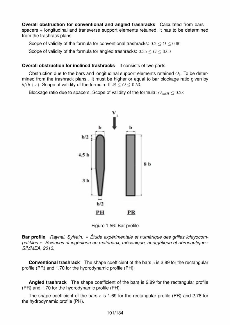
Overall obstruction for conventional and angled trashracks Calculated from bars +spacers + longitudinal and transverse support elements retained, it has to be determinedfrom the trashrack plans.
Scope of validity of the formula for conventional trashracks: 0.2 ≤ O ≤ 0.60
Scope of validity of the formula for angled trashracks: 0.35 ≤ O ≤ 0.60
Overall obstruction for inclined trashracks It consists of two parts.
Obstruction due to the bars and longitudinal support elements retained Ob. To be deter-mined from the trashrack plans.. It must be higher or equal to bar blockage ratio given byb/(b+ e). Scope of validity of the formula: 0.28 ≤ O ≤ 0.53.
Blockage ratio due to spacers. Scope of validity of the formula: OentH ≤ 0.28
Figure 1.56: Bar profile
Bar profile Raynal, Sylvain. « Étude expérimentale et numérique des grilles ichtyocom-patibles ». Sciences et ingénierie en matériaux, mécanique, énergétique et aéronautique -SIMMEA, 2013.
Conventional trashrack The shape coefficient of the bars a is 2.89 for the rectangularprofile (PR) and 1.70 for the hydrodynamic profile (PH).
Angled trashrack The shape coefficient of the bars is 2.89 for the rectangular profile(PR) and 1.70 for the hydrodynamic profile (PH).
The shape coefficient of the bars c is 1.69 for the rectangular profile (PR) and 2.78 forthe hydrodynamic profile (PH).
101/134

inclined trashrack The shape coefficient of the bars a is 3.85 for the rectangular profile(PR) and 2.10 for the hydrodynamic profile (PH).
Average shape coefficient of spacers and transverse elements, weighted accordingto their respective shares
inclined trashrack To be determined from the trashrack plans.
For example, 1.79 for cylindrical spacers, 2.42 for rectangular spacers, and around 4 forsquare beams and IPNs.
1.9.2 Jet impact
This module performs a ballistic calculation of a jet while neglecting air friction. It allows tocalculate the missing value among the following quantities:
• Initial velocity at the start of the jet (m/s)
• Initial slope at the start of the jet (m/m). Note that, contrary to the slope used in thefree surface calculation module, this slope is positive for an upward directed jet andnegative for a downward directed jet.
• Abscissa of the impact or horizontal distance travelled between the start of the jet andthe point of impact (m)
• Start dimension of the jet (m)
• Water elevation (m)
The bottom elevation is used to calculate the depth and the depth to fall ratio.
1.9.2.1 Designing an outlet for fish evacuation
The downstream fish evacuation outlet ends with a device that empties into the plant’s tail-race. This module calculates the position and velocity at the point of impact of the free fallor water vein on the surface of the tailrace water taking into account the initial angle andvelocity of the jet and the drop height.
Excerpt from Courret, Dominique, and Michel Larinier. Guide for the design of ichthy-ocompatible water intakes for small hydroelectric power plants, 2008. https://doi.org/10.13140/RG.2.1.2359.1449,p.24:
Speeds in the structure and at the point of impact in the tailrace must remainbelow about 10 m/s, with some organizations even recommending that they notexceed 7-8 m/s (ASCE 1995). (. . . ) The head between the outlet and the waterbody must not exceed a dozen metres to avoid any risk of injury to fish on impact,whatever their size and mode of fall (free fall or fall in the water vein) (Larinierand Travade 2002). The discharge must also be made in an area of sufficientdepth to avoid any risk of injury from mechanical shock. Odeh and Orvis (1998)recommend a minimum depth of about a quarter of the fall, with a minimum ofabout 1 m.
102/134

1.9.2.2 Formulas used
Fall height
H = 0.5 ∗ g ∗ D2
cosα2 ∗ V 20
− tanα ∗D
With:
• H: height of fall (m) which corresponds to the difference in height between the jet’sdeparture and the water surface.
• g: acceleration of gravity = 9.81 m.s-2
• D: horizontal distance travelled between the start of the jet and the point of impact (m)
• α : angle of shooting in relation to the horizontal (°)
• 0 : initial speed (m/s)
Impact abscissa (horizontal distance covered)
D =V0
g ∗ cosα
(V0 ∗ sinα +
√(V0 ∗ sinα)2 + 2 ∗ g ∗H
)
Flight time
t =D
V0 cosα
Horizontal speed at impactVx = V0 cosα
Vertical speed at impactVz = V0 sinα− t ∗ g
Speed at impactVt =
√V 2x + V 2
z
1.10 Mathematical tools
1.10.1 Operators and trigonometric functions
The basic mathematical operators and functions provided by Cassiopeia make it possibleabove all to facilitate the link between the results of one calculation module and the input intoanother in the case of a sequence of calculations between several modules. The providedexample “Weir jet length” shows the use of the “Linear function” module.
103/134

1.10.1.1 Linear function
The linear function module solves the equation of a line:
y = ax+ b
Three parameters must be entered and the module calculates the missing parameter.
1.10.1.2 Sum and product of powers
This module allows to write an equation summing powers in the form axn with a, x, and n ofreal numbers.
In the case of a sum the equation solved by the module is written:
y =k∑i=1
aixnii
In the case of a product the equation solved by the module is written:
y =k∏i=1
aixnii
All parameters must be entered except the last one which is the value calculated in theequation.
1.10.1.3 Trigonometric function
This module allows to calculate the value of a trigonometric function or its inverse.
The equation solved by this module is written:
y = f(x)
With f , a trigonometric function and x an angle in degrees or radian.
The “Operation” parameter allows to choose the operator among the available functions:cos, sin, tan, cosh, sinh and tanh. The “Unit” parameter is used to choose between degreeand radian.
1.10.2 Multi-module solver
The multi-module solver allows to calculate the value of an input parameter of a moduledepending on a calculation chain made up of several modules for which a target value for anoutput calculated parameter is sought.
The diagram below shows the example of a calculation chain comprising two modules.The module x takes the parameter Input x and calculates the parameter Output x. They module takes the Input y parameter and calculates the Output y parameter. The
104/134

Input y parameter is linked to the Output x parameter. The problem to be solved by thesolver is to get the value of the Input x to obtain a target value in Output y.
graph LRIx([Input x])x[Module x]Ox([Output x / Input y])y[Module y]Oy([Output y])Ix --> xx --> OxOx --> yy --> OyOy -..->|Input x for a target value Output y ?| Ix
To solve this problem, the characteristics of the target parameter must be defined whichinclude:
• The module and its calculated parameter (here the module y calculating Output y);
• The target result which can be the parameter calculated by the module or one of itscomplementary results (Here Output y);
• The desired target value.
It is also necessary to define the characteristics of the searched parameter:
• The searched parameter is to be chosen from the list of input parameters of the mod-ules of the session (Here the Input x parameter of the x module);
• An initial value of this parameter to start the calculation.
The initial value chosen must be close enough to the solution because there is noguarantee that the function resulting from the sequence of calculations is continuous andmonotonous.
Examples of the use of the multi-module solver are given in the example sessions “Chan-nel flow with structures” and “Critical slope of a channel”. The notes of these sessionsdescribe the sequence of the modules and the use of the solver.
1.11 Numerical methods
1.11.1 Runge-Kutta diagram of order 4
The Runge-Kutta scheme of order 4 is based on an approximation of the derivative to ahigher order (order 4). The principle of discretization is the same as for the Euler method,but we will make some additional calculations to approach the derivative:
• we know the function f , a point ti where we know yi
105/134

• we can therefore calculate f1 = y′i = f(yi, ti) (cf. Euler=pente method to the point(ti, yi))
• we calculate f2 = f(yi + 12∆tf1, ti + 1
2∆t) (estimated value in the middle of the interval,
with the slope taken in ti)
• we calculate f3 = f(yi + 12∆tf2, ti + 1
2∆t) (estimated value in the middle of the interval
ti+1/2, with the slope taken in ti+1/2
• we calculate f4 = f(yi + ∆tf3, ti + ∆t) (estimated value in ti+1, with the slope taken inti+1/2
• we then have yi+1 ' y1 + 16∆t(f1 + 2f2 + 2f3 + f4)
• you can then iterate (solve step by step) to move to the next point. The problem isinitialized from t0 where we know y0 (boundary condition).
It is clear that the method is much more precise. Even with a much higher calculationstep, the solution is approached correctly, whereas the Euler method gives results very farfrom the exact solution. We also note that, between the discretization points, the solutionwas approached by line segments (although we may have more advanced interpolation ifwe need to know intermediate values).
The program can be written as follows, using the Scilab scientific calculation software:
// Program for solving a differential equation// Equation to be solved: dy/dt=f(y,t)
// Definition of the function fa=-0.1;function z=f(y,t);z=a*y; endfunction
// Boundary condition:t0=0;y0=1;
// Time discretizationtmax=50;dt=5;
// Number of discretization stepsN=(tmax-t0)/dt;// Indicesii=1:N+1;t=(ii-1)*dt; // time vector
// time vector with a finer step, for the exact solutiont2=0:tmax;
// Solution by Euler method, noted yeye(1)=y0; // boundary conditionfor i=1:N
106/134
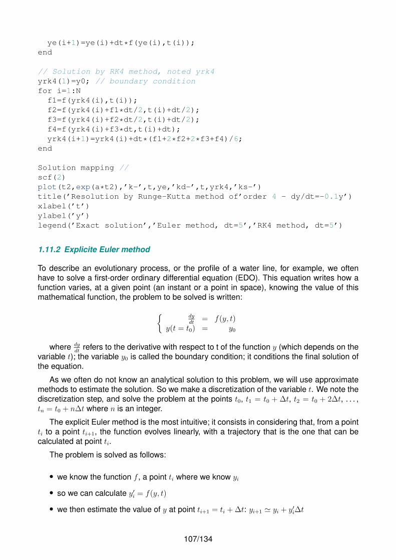
ye(i+1)=ye(i)+dt*f(ye(i),t(i));end
// Solution by RK4 method, noted yrk4yrk4(1)=y0; // boundary conditionfor i=1:N
f1=f(yrk4(i),t(i));f2=f(yrk4(i)+f1*dt/2,t(i)+dt/2);f3=f(yrk4(i)+f2*dt/2,t(i)+dt/2);f4=f(yrk4(i)+f3*dt,t(i)+dt);yrk4(i+1)=yrk4(i)+dt*(f1+2*f2+2*f3+f4)/6;
end
Solution mapping //scf(2)plot(t2,exp(a*t2),’k-’,t,ye,’kd-’,t,yrk4,’ks-’)title(’Resolution by Runge-Kutta method of’order 4 - dy/dt=-0.1y’)xlabel(’t’)ylabel(’y’)legend(’Exact solution’,’Euler method, dt=5’,’RK4 method, dt=5’)
1.11.2 Explicite Euler method
To describe an evolutionary process, or the profile of a water line, for example, we oftenhave to solve a first-order ordinary differential equation (EDO). This equation writes how afunction varies, at a given point (an instant or a point in space), knowing the value of thismathematical function, the problem to be solved is written:{
dydt
= f(y, t)y(t = t0) = y0
where dydt
refers to the derivative with respect to t of the function y (which depends on thevariable t); the variable y0 is called the boundary condition; it conditions the final solution ofthe equation.
As we often do not know an analytical solution to this problem, we will use approximatemethods to estimate the solution. So we make a discretization of the variable t. We note thediscretization step, and solve the problem at the points t0, t1 = t0 + ∆t, t2 = t0 + 2∆t, . . . ,tn = t0 + n∆t where n is an integer.
The explicit Euler method is the most intuitive; it consists in considering that, from a pointti to a point ti+1, the function evolves linearly, with a trajectory that is the one that can becalculated at point ti.
The problem is solved as follows:
• we know the function f , a point ti where we know yi
• so we can calculate y′i = f(y, t)
• we then estimate the value of y at point ti+1 = ti + ∆t: yi+1 ' yi + y′i∆t
107/134
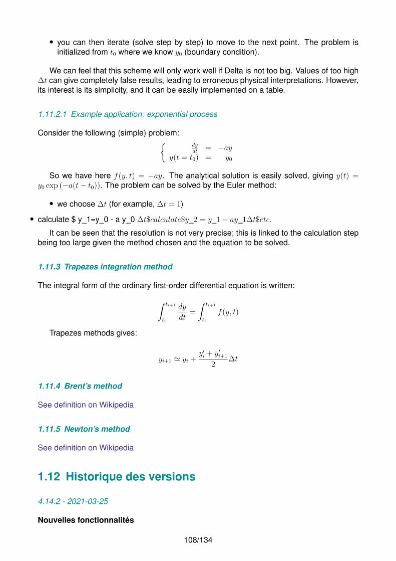
• you can then iterate (solve step by step) to move to the next point. The problem isinitialized from t0 where we know y0 (boundary condition).
We can feel that this scheme will only work well if Delta is not too big. Values of too high∆t can give completely false results, leading to erroneous physical interpretations. However,its interest is its simplicity, and it can be easily implemented on a table.
1.11.2.1 Example application: exponential process
Consider the following (simple) problem:{dydt
= −ayy(t = t0) = y0
So we have here f(y, t) = −ay. The analytical solution is easily solved, giving y(t) =y0 exp (−a(t− t0)). The problem can be solved by the Euler method:
• we choose ∆t (for example, ∆t = 1)
• calculate $ y_1=y_0 - a y_0 ∆t$calculate$y_2 = y_1− ay_1∆t$etc.
It can be seen that the resolution is not very precise; this is linked to the calculation stepbeing too large given the method chosen and the equation to be solved.
1.11.3 Trapezes integration method
The integral form of the ordinary first-order differential equation is written:
∫ ti+1
ti
dy
dt=
∫ ti+1
ti
f(y, t)
Trapezes methods gives:
yi+1 ' yi +y′i + y′i+1
2∆t
1.11.4 Brent’s method
See definition on Wikipedia
1.11.5 Newton’s method
See definition on Wikipedia
1.12 Historique des versions
4.14.2 - 2021-03-25
Nouvelles fonctionnalités
108/134

•• Passe à macro-rugosité: Retour aux formules utilisées dans la v4.13.1 (jalhyd#297,nghyd#493)
Correction de bogues
• Passe à macro-rugosité: error de calcul de la vitesse max (jalhyd#294)
• Graphiques: lorsqu’on relance un calcul les axes ne se mettent pas à jour (nghyd#489)
Documentation
• Macrorugo : Documentation de Cd0 avec schéma (nghyd#492)
4.14.1 - 2021-02-17
Nouvelles fonctionnalités
• Passe à macro-rugosité: Changer Cd0 pour Cx et ajuster Cd0 aux données expéri-mentales (jalhyd#291)
Correction de bogues
• Vérificateur de passe: message erroné pour les passes à macro-rugosités submergées(jalhyd#292)
4.14.0 - 2021-02-16 (Scomber scombrus)
Nouvelles fonctionnalités
• Passe à macro-rugosité: Mise à jour des formules de calcul (jalhyd#283)
• Passe à macro-rugosité: Ajout de la vitesse moyenne entre les blocs (jalhyd#285)
• Passe à macro-rugosité: Ajout du Strickler équivalent dans les résultats liables à desStrickler (jalhyd#287)
• Passe à macro-rugosité: ajout d’un avertissement pour les concentrations en dehorsde l’intervalle validé par les expérimentations (jalhyd#284)
• Vérificateur: Les passes à macro-rugosité submergées sont non franchissables (jal-hyd#290)
Correction de bogues
• Passe à macro-rugosité: Calcul de la puissance dissipée erroné (jalhyd#282)
• Crash au chargement d’un module contenant une parenthèse dans son nom (nghyd#487)
• Electron: l’icône de l’application n’est plus reconnue (nghyd#485)
109/134

Documentation
• Documentation du solveur multi-module et des modules de calcul mathématiques(nghyd#433)
• Macrorugo : documenter le coefficient de forme Cd0 (nghyd#477)
• MacroRugo: erreur de formule de correction de Cd dans la documentation (nghyd#488)
• Documentation du module de calcul de la cote amont / aval d’un bief (nghyd#490)
4.13.1 - 2020-10-02
Correction de bogues
• PreBarrage: Distribution des débits erronée sur exemple simple (jalhyd#279)
• PreBarrage: erreur de calcul sur Z2 > Z1 initiale (jalhyd#280)
• Prebarrage : avec Chrome (et electron) le schéma est mal rendu (nghyd#482)
4.13.0 - 2020-09-24 (Michel Larinier)
Nouvelles fonctionnalités
• Module Pré-barrage (jalhyd#32, jalhyd#269, jalhyd#268, jalhyd#243, jalhyd#246, nghyd#395,nghyd#430, nghyd#456, nghyd#455, jalhyd#275, jalhyd#276, jalhyd#277, jalhyd#278,nghyd#452, nghyd#470, nghyd#451)
• Simplification de l’architecture des composants de résultats Angular (nghyd#418, nghyd#466,nghyd#465)
• Modifier les titres et descriptions de “Passes à bassins” et “Passes à macro-rugosités”(nghyd#478)
• Ajouter des mots-clés “maths” pour les outils mathématiques (moteur de recherche)(nghyd#474)
Correction de bogues
• Electron : la détection de mise à jour disponible ne fonctionne plus (nghyd#462)
• Débit lié au débit en calcul d’un PréBarrage : erreur dans CalcSerie() (jalhyd#274)
• Cloisons : changer le type d’ouvrage pour Seuil Triangulaire casse le fieldset (nghyd#479)
Documentation
• Prébarrages (nghyd#467)
• Aide du Jet / de la pente : mentionner l’inversion de la pente pour le module Jet(nghyd#475)
• Ajouter à l’accueil de la documentation un chapitre “contact, bugs, remarques. . . ”(nghyd#472)
110/134
4.12.1 - 2020-09-15
Correction de bogues
• Lien vers la documentation cassé sur Chrome et Edge (nghyd#458)
• Macrorugo : en mode “champs vides par défault”, L est en calcul avec une valeurinitiale vide (nghyd#459)
• Grille : différencier Ob de O pour les grilles inclinées (jalhyd#273)
• Fermeture d’un module Jet calculé : plante l’application (nghyd#460)
• Déversoir dénoyé : Infinity pour des largeurs de lit faible et sur variation (jalhyd#272)
Documentation
• Lechapt-Calmon : documentation du coefficient de pertes de charges singulières (nghyd#338)
4.12.0 - 2020-09-09 (Les critères de Francis Blanche ils peuvent le faire !)
Nouvelles fonctionnalités
• Vérification des critères de franchissement des passes à poissons (jalhyd#204, nghyd#60,jalhyd#236, jalhyd#251, jalhyd#238, jalhyd#252, jalhyd#250, jalhyd#258, jalhyd#247,jalhyd#239, jalhyd#249, jalhyd#248, jalhyd#254, jalhyd#235, jalhyd#237, nghyd#402,jalhyd#216, nghyd#426)
• Moteur de recherche sur la page d’accueil (nghyd#428)
• Améliorer le système de traduction (nghyd#223)
• Labels des paramètres : lire l’unité dans le modèle et non dans les fichiers de traduc-tion (nghyd#417)
• Cloisons : remplacement de la loi Cunge80 par la loi CEM88D (jalhyd#264)
Correction de bogues
• Cordova : la notification de mise à jour ne fonctionne plus (nghyd#436)
• Conditionner le passage en mode CALC aux liens déjà définis, pour éviter les boucles(nghyd#181)
• Solveur : le paramètre recherché, si c’est un extraResult, ne s’initialise pas correcte-ment lors du chargement d’une session (jalhyd#263)
• Solveur : this.prms.X is undefined (jalhyd#262)
• Exemple “débit d’un chenal avec ouvrages” : plusieurs bugs (nghyd#446)
• PAR, générer une simulation à partir d’un calage : NaN (nghyd#447)
111/134

• Paramètres liés d’un enfant à l’autre d’un même module : boucle infinie si la sourcevarie (nghyd#444)
• JaLHyd : dans createStructure(), définir automatiquement le structureType en fonctionde la loiDebit
• Lors de la vérification d’une passe à bassins variée, bug sur la vérification de chargeminimale (jalhyd#265)
• PAB, calcul de cloison qui échoue : l’erreur ne dit pas quelle cloison est en cause(jalhyd#267)
• Vérification d’une PAB variée : erreur dans la vérification des critères obligatoires (jal-hyd#266)
• Vérification de PAB : rendre la largeur minimale d’échancrure obligatoire (jalhyd#270)
Documentation
• Documentation de la vérification des passes (nghyd#434)
• Traduire la documentation des PAR (nghyd#443)
• Harmonisation de l’indentation des fichiers (nghyd#409)
Mises à jour de dépendances
• Angular 10
• Cordova 10
• Electron 10
• Mathjax 3 (nghyd#416)
4.11.1 - 2020-08-11
Nouvelles fonctionnalités
• Lois d’ouvrages: ajouter le n° d’ouvrage dans les logs (jalhyd#260, nghyd#442)
Correction de bogues
• Erreur de formulation de la loi de Cunge en orifice dénoyé (jalhyd#259)
• Définition de la valeur initiale d’un calcul (nghyd#440)
• Structure et Dever : exposer les résultats pour liage (jalhyd#255)
• Déversoirs dénoyés: Ajouter les liens vers les lois de débit (nghyd#437)
112/134

Documentation
• Mise à jour de la documentation de la loi de Cunge (nghyd#441)
4.11.0 - 2020-07-28 (Puisque tu PAR)
Nouvelles fonctionnalités
• Calage d’une passe à ralentisseurs (jalhyd#34, jalhyd#223, jalhyd#225, jalhyd#226,jalhyd#232, jalhyd#233, jalhyd#234, jalhyd#240, nghyd#365, nghyd#394, nghyd#408,nghyd#422, nghyd#423, nghyd#424, nghyd#425)
• Simulation d’une passe à ralentisseurs (jalhyd#201, jalhyd#229, nghyd#366, nghyd#382,nghyd#394, nghyd#425)
• Bief : lier les paramètres de section pour les Sections Paramétrées générées (nghyd#380)
• Permettre de lier des paramètres de sections de types identiques, sans utiliser lesfamilles (jalhyd#203, nghyd#379)
Correction de bogues
• Lien entre deux paramètres de section : la valeur n’apparaît pas dans le tableau derésultats (nghyd#381)
• Désactiver le suivi Matomo lorsqu’Angular n’est pas en mode “prod” (nghyd#412)
• Corriger le coefficient de débit de la vanne submergée (jalhyd#231, nghyd#421)
• Cloisons : une pelle (négative) est calculée pour les orifices, ce qui donne lieu à desavertissements (jalhyd#242)
• Empêcher de créer des liens vers des paramètre invisibles (jalhyd#244)
• MRC : après un calcul varié, il n’y a plus d’eau sur certains radiers (jalhyd#253,nghyd#432)
Documentation
• Passes à ralentisseurs (nghyd#398)
4.10.6 - 2020-07-21
Nouvelles fonctionnalités
• Transférer les fonctionnalités de cassiopee-2-integration dans Gitlab-CI (nghyd#374)
Correction de bogues
• Lechapt-Calmon : ne plus proposer de matériau “NONE” (jalhyd#230)
113/134
Documentation
• Renommer les lois d’ouvrage (nghyd#419)
• Erreur dans l’équation de Cunge
• Corrections mineures sur Vanne Dénoyée
4.10.5 - 2020-06-30
Nouvelles fonctionnalités
• Renommer les lois triangulaires “dénoyées” en “(Villemonte)” (jalhyd#210, nghyd#393)
• Lois d’ouvrages: ajout du seuil triangulaire épais (jalhyd#211, nghyd#399)
• Régime Uniforme, conduite circulaire: provoquer une erreur fatale si la conduite est encharge (jalhyd#214, nghyd#406)
• Cunge 1980 : ajout dans les cloisons et modification du coefficient de débit à 1 (jal-hyd#220, jalhyd#221, nghyd#404)
Correction de bogues
• PAB : résultats cassés (nghyd#392)
• PAM : Supprimer le lien rugosité de fond (nghyd#391)
• Cloisons : avertissement si les cotes de radier des seuils se situent sous la cote deradier du bassin amont (jalhyd#217)
• Absence d’erreur en cas de code de langue manquant dans les listes déroulantes(nghyd#400)
• Contrôler le domaine de définition lors de l’affectation de .singleValue (jalhyd#218)
• Ouverture de vanne et liens : bug sur longueur du paramètre varié (jalhyd#222)
• Exemple “Longueur de jet d’un déversoir” cassé (jalhyd#224)
• Exemple 3 : l’affichage de graphique clignote (nghyd#407)
• Définition de la pente (jalhyd#212)
Documentation
• Documentation de la pente (nghyd#397)
• Documentation de la loi Cunge80 (nghyd#403)
• Documentation des grilles: il manque la définition des variables (nghyd#401)
114/134

4.10.4 - 2020-04-17
Nouvelles fonctionnalités
• Régime uniforme: ajouter un bouton pour créer une section paramétrée (nghyd#386)
• Cordova : notifications de mise à jour (nghyd#384)
Correction de bogues
• Section paramétrée: le tirant d’eau critique ne converge pas sur une section circulairefermée (jalhyd#209)
• Régime uniforme: erreur de calcul de la vitesse (jalhyd#206, jalhyd#207)
• Impact de jet: problème de gestion des erreurs fatales (jalhyd#205)
• Unité du coefficient de Strickler (jalhyd#208)
• Robustifier le solveur sur la recherche de l’intervalle de départ (jalhyd#164)
• Champ vide à la création d’un module: les champs de section ne sont pas vides quandon choisit un type de section (nghyd#388)
• Section paramétrée: Ajouter le tirant d’eau dans le schéma en coupe de la section(nghyd#389)
• Saisie paramètre qui varie: message d’erreur persistant sur le champ min (nghyd#385)
• Cordova : version erronée (nghyd#383)
Documentation
• Fusionner “Section paramétrée” et “Variables hydrauliques” (nghyd#390)
• Sections : documentation du champ Hauteur de berge
4.10.3 - 2020-03-12
Nouvelles fonctionnalités
• Nouveau raccourci clavier Alt+G pour afficher le diagramme des modules
• Diagramme des modules : lien vers les notes
• Test e2e des exemples officiels (nghyd#373)
• Exemples types mis à jour, avec notes
115/134

Correction de bogues
• Calcul d’un module aval qui casse les résultats du module amont (nghyd#371)
• Astérisques sur les champs non-obligatoires (nghyd#368)
• Exemple “Débit d’un chenal avec ouvrages” : impossible de calculer la cote amontdans le module “Cotes d’un bief” (jalhyd#202)
• Déversoirs et Lois d’ouvrages : liens erronés vers la documentation du seuil dénoyé
• Jet : ne pas remplir “sous” la ligne de fond, lorsque sa cote est négative (nghyd#372)
• Passage en mode calcul d’un paramètre dont la singleValue est undefined (nghyd#367)
• Marges sur les titres de Fieldset, Fieldset container, PAB Table
• Désactivation des notifications lorsqu’on vide la session (nghyd#375)
• Chargement d’un Solveur avant ses Nubs cibles
• Sélection de la cible du Solveur lorsque le Nub calculé n’a pas de paramètre calculé(ex: Section Paramétrée) (nghyd#378)
• Section Paramétrée : tableau de résultats fixes en plusieurs exemplaires lors de l’utilisationavec le Solveur (nghyd#377)
• Bief : calcul des sections amont et aval (nghyd#376)
4.10.2 - 2020-02-25
Correction de bogues
• Correction de liens erronés vers la documentation
Documentation
• Documentation : ajout de liens vers la page de téléchargement
4.10.1 - 2020-02-25
Correction de bogues
• Electron : erreur de détection de mise à jour (comparaison chaînes semver)
116/134

4.10.0 - 2020-02-24 (Langue Hilare Neuve)
Nouvelles fonctionnalités
• Solveur : cibler un résultat complémentaire (nghyd#363, jalhyd#188)
• Monkey test sur les interfaces (nghyd#235)
• Lechapt-Calmon : ajouter un avertissement lorsque la vitesse est en dehors de l’intervalle[0.4, 2] (jalhyd#192)
• Rendre plus générique la gestion des listes déroulantes (nghyd#359)
• Automatiser les chemins de configuration depuis le CalculatorType (nghyd#358)
Correction de bogues
• Certains liens doivent être cliqués deux fois (nghyd#364)
• Solveur : interdire de travailler sur un Nub dont le résultat est varié (jalhyd#198)
• Paramètre varié et lien à un résultat varié simultanément (jalhyd#199)
• Parfois lorsqu’on charge une session, le bouton Calculer reste grisé (nghyd#349)
• PAB : parfois le type de jet est undefined (jalhyd#196)
• Export XLSX : retirer “help” des entêtes de colonnes (nghyd#360)
• Chargement de session : selon l’ordre des paramètres, le paramètre calculé n’est pascorrectement défini
Documentation
• Générer la documentation en PDF (nghyd#348)
Mises à jour de dépendances
• Angular 9 (nghyd#354)
• Typescript 3.7 (jalhyd#197)
• mise à jour de toutes les dépendances jalhyd/nghyd sauf Mermaid (provoque un bug)et Mathjax (adaptations importantes nécessaires)
4.9.0 - 2020-01-15 (On Fusionne Bien)
Nouvelles fonctionnalités
• Nouveau module “Concentration de blocs” (jalhyd#185)
• Lechapt-Calmon : ajout des pertes de charge singulières (nghyd#352, jalhyd#172)
• Simplification du code des Formulaires (nghyd#353)
• Passage de l’AFB à l’OFB : changement de logo, de nom, d’URL
117/134
Documentation
• Documentation utilisateurs en anglais (nghyd#321)
• Réorganisation de la documentation utilisateurs (nghyd#355)
• Documentation développeurs (nghyd#317)
• Exemples de code Typescript et Javascript pour le développement d’applications enligne de commande basées sur JaLHyd
• Diagramme de classes simplifié de JaLHyd
Mises à jour de dépendances
• Jasmine 3.5
• Karma 4.4
4.8.1 - 2019-12-20
Nouvelles fonctionnalités
• Dever: Ajout d’un avertissement si la cote de radier d’un ouvrage est sous la cote defond du lit (jalhyd#179)
• Strickler: Ajout d’une aide contextuelle (nghyd#332)
• Grille: permettre les calculs partiels (nghyd#336)
• MacroRugo: Ajout d’avertissement sur l’adéquation taille des cellules - largeur de larampe (jalhyd#174)
• Documentation lois d’ouvrages manquantes (nghyd#342)
• Champs vides à la création d’un module (nghyd#331)
• Dever: Calcul du débit corrigé en utilisant la charge dans les formules (jalhyd#52,nghyd#345)
• Grille: Ajouter le coefficient de forme des barreaux dans les résultats complémentaires(jalhyd#178)
• Grille: Ajouter un profil de barreaux personnalisé (nghyd#334)
• PAB: Ajouter la position du radier des seuils sur le graphique du profil en long (jal-hyd#171)
• Impact de jet: Modification des champs de hauteurs (jalhyd#181)
• Hydraulique à surface libre: ajouter un avertissement quand ça déborde (jalhyd#180)
• Cloisons: Ajouter le calcul de la pelle (jalhyd#169)
• MacroRugoCompound: radier incliné - Ajouter le calcul du dévers latéral (jalhyd#177)
118/134
• MacroRugo: Supprimer les débits et vitesses du guide technique (jalhyd#177)
• MacroRugo: Domaine de définition de Cd0 (jalhyd#175)
• PAB nombre: Ajout du nombre de chutes harmonisé (jalhyd#167)
• MacroRugoComplexe: modification du libellé des champs (nghyd#333)
• PAB: Export du tableau de géométrie au format XLSX (jalhyd#170)
• MacroRugo: transition douce entre régime émergent et régime submergé (jalhyd#191)
Correction de bogues
• Parfois, lorsque le débit varie, la PAB n’a pas d’eau à l’aval pour certaines valeurs dedébit (jalhyd#187)
• Lorsqu’on vide un champ, si on change de page, au retour le champ est à nouveaurempli (nghyd#343)
• Impact de chute: Erreur de calcul de la chute nécessaire pour atteindre l’abscissed’impact (jalhyd#183)
• Impact de jet: non prise en compte de l’angle (jalhyd#182)
• Grille: Pas d’invalidation des résultats sur le choix du profil des barreaux (nghyd#335)
• MacroRugoCompound: radier incliné - changer la répartition des cellules (jalhyd#173)
4.8.0 - 2019-11-26 (Affine et forte à la fois, par amour du remous)
Nouvelles fonctionnalités
• Module Fonction affine (jalhyd#160, nghyd#319)
• Module Trigonométrie (jalhyd#161)
• Module Somme et produit de puissances (jalhyd#162)
• Loi Déversoir noyé (jalhyd#165, nghyd#318)
• Logo animé lors du chargement de l’application (nghyd#322)
Correction de bogues
• MacroRugo: définition de la valeur par défaut de Cd0 à 1.2 (jalhyd#166)
• Échec du calcul en chaîne dans certains cas (nghyd#325)
• Remous : suppression de LargeurBerge dans le log (nghyd#326)
• Remous : les tirants d’eau critique et normal sont erronés sur le graphique (nghyd#327)
• Remous : une fois calculé, chaque rechargement du module ajoute une copie des logs(nghyd#324)
• Remous : en fluvial uniquement avec forte pente, les abscisses sont fausses (nghyd#328)
• Calcul en chaîne : ERR inopiné dans le tableau de résultats fixes (nghyd#329)
119/134
4.7.0 - 2019-10-29 (AGB - Agence Grolandaise pour la Biodiversité)
Nouvelles fonctionnalités
• Solveur multi-modules (jalhyd#152, nghyd#301)
• Nouvelle loi d’ouvrage: Orifice Dénoyé (jalhyd#156, nghyd#311)
• Script de déploiement d’une nouvelle version (sur Aubes) (cassiopee2-integration#9)
• Documentation lois d’ouvrages CEM88 V et D (nghyd#315)
• Remous: connecter le ressaut sur un seul point lorsque le ressaut est court (une seuleabscisse) (nghyd#312)
Correction de bogues
• Lois d’ouvrages: bug à l’affichage des résultats variés lorsque le calcul échoue (jal-hyd#163)
• PAB : problème de cotes sur les cloisons (jalhyd#158)
• Calcul en chaîne: stopper la chaîne si une erreur survient (jalhyd#155)
• Diagramme de Jet / de Section : problème de rafraîchissement (nghyd#308)
• Remous : il manque parfois une abscisse (jalhyd#147)
Mises à jour de dépendances
• chartjs-plugin-zoom 0.7.4
4.6.1 - 2019-10-15
Nouvelles fonctionnalités
• Suivi des comportements des utilisateurs à l’aide de Matomo (sur Aubes) (nghyd#306)
• Documentation: faciliter l’accès à l’application plutôt qu’à GitLab (nghyd#307)
Mises à jour de dépendances
• chartjs-plugin-zoom 0.7.4
120/134
4.6.0 - 2019-10-14 (Bluefish délavé)
Nouvelles fonctionnalités
• Ajout du module Bief (jalhyd#55, nghyd#299)
• Ajout du module Grille (jalhyd#114, nghyd#289)
• Ajout du module Impact de Jet (jalhyd#112, nghyd#287)
• Ajout du module : Pente (jalhyd#143, nghyd#295)
• Passage des courbes de remous en cotes (jalhyd#146, nghyd#298)
• SectionParametree: remplacement de Yf et Yt par Ycor (jalhyd#145, nghyd#297)
• Régime uniforme: ajout de la vitesse moyenne (jalhyd#139)
• Page d’accueil: ajout du logo du pôle (IMFT), remplacement du texte nghyd#208)
• Tests e2e sur les messages de langues absents (nghyd#294)
• Ajout de la possibilité d’un bouton d’aide dans les résultats (nghyd#293)
• Electron : mise à jour automatique (nghyd#250)
• Intégration continue : exécution des tests e2e (nghyd#278)
• Préférences: applicaton de “precision” et “newtonMaxIter” à la Session en cours (jal-hyd#40, nghyd#286)
• Lorsqu’un paramètre varie, ajout dans le log global d’un résumé des erreurs/avertissements(jalhyd#140)
Correction de bogues
• MacroRugo: écart des débits en submergé (jalhyd#154)
• MacroRugo: non convergence du calcul pour les faibles profondeurs (jalhyd#144)
• Remous : crash avec paramètre lié à un résultat non calculé (jalhyd#151)
• Remous : lorsque la longueur du bief n’est pas un multiple du pas de discrétisation,exécuter le calcul sur la dernière abscisse tout de même (jalhyd#153)
• Remous: parfois le premier point de la courbe torrentielle est absent (jalhyd#148)
• Cordova: le zoom sur les graphiques n’est pas réinitialisable (nghyd#270)
• Chargement de session : déduire le type de structure (nodeType) de la loi de débit(nghyd#265)
• Lechapt-Calmon : effacer les résultats lorsqu’on change de matériau (nghyd#291)
• Lois d’Ouvrages: les logs ne s’affichent pas (jalhyd#120, nghyd#284)
• Lois d’ouvrages: calculer un paramètre enfant en variant la cote aval fait planter lesrésultats (nghyd#285)
121/134
Mises à jour de dépendances
• chartjs-plugin-zoom 0.7.4
• ngx-markdown 8.2.1
• electron 6.0.10
4.5.0 - 2019-09-09 (Fish ramps that rock!)
Nouvelles fonctionnalités
• Passe à macro-rugosité complexe (jalhyd#35, nghyd#271)
• Réorganisation des onglets par glisser-déposer (nghyd#206)
• Raccourcis clavier (nghyd#192)
• Ajout des graphiques de type “Points” (nghyd#118)
• Passe à bassins: Supprimer simultanément plusieurs bassins (nghyd#269)
• Sessions exemples (nghyd#165)
• Diagrammes des modules de calcul et de leurs liens (nghyd#140)
• Amélioration de la précision d’affichage (nghyd#281, nghyd#29)
• Ouverture d’un fichier de session pour chargement : prévenir si le fichier est vide oumal formé (nghyd#264)
Correction de bogues
• Lechapt-Calmon : le sélecteur de matériaux n’a plus de sélection par défaut (nghyd#276)
• Lechapt-Calmon : enregistrement de la propriété “matériaux” (jalhyd#138)
• Lois d’ouvrages: plantage sur deux paramètres qui varient (nghyd#273)
• Passe à bassins: prise en compte de la longueur des bassins dans l’interpolation(nghyd#268)
• Passe à bassins: il manque l’édition de la cote de radier de la cloison aval (nghyd#277)
• Résultats fixés: l’unité des paramètres calculés n’est pas affichée (nghyd#274)
122/134

4.4.2 - 2019-08-06
Nouvelles fonctionnalités
• Boutons d’aide sur tous les éléments graphiques (nghyd#157)
• Chargement de session: ouverture automatique du premier module nouvellementchargé
• Touche Tab dans un champ de saisie: le texte est surligné (nghyd#259)
• Simplification des fichiers de session
• Graphique : afficher tous les paramètres d’une même famille simultanément (nghyd#246)
• Réorganisation du format des résultats (jalhyd#128)
• Erreur au chargement de session avec lien sur des paramètres calculés (nghyd#263)
• Enregistrement de session partielle avec liens tronqués: enregistrer les valeurs courantesdes paramètres (jalhyd#133)
Correction de bogues
• Documentation de la passe à Macrorugosités
• Enregistrement de session: dédoublonner les messages concernant les dépendances
• nodeType est lu depuis la Section et plus depuis le Nub parent (jalhyd#124)
• Electron / Cordova : script npm pour mettre à jour les mimetypes dans dist/index.html(nghyd#258)
• Passe à bassins : traduction
• Graphiques : ne pas représenter les données de type ENUM (nghyd#260)
• Remous : l’itérateur d’abscisses est en retard sur le dessin du graphe (nghyd#267)
4.4.1 - 2019-07-30
Nouvelles fonctionnalités
• Passe à bassins : ajouter un accès rapide aux différents panneaux (table, résultats,graphiques. . . ) pour éviter de faire défiler péniblement (nghyd#237)
• Passe à bassins : permettre d’ajouter / dupliquer un ouvrage pour plusieurs cloisons àla fois (nghyd#243)
• Passe à bassins : ajouter la nature du jet (nghyd#245)
• Lois d’ouvrages: Ne pas écraser les valeurs par défaut du coefficient de débit auchangement de loi (nghyd#225)
• Lois d’ouvrages: Ajouter le type de jet dans les résultats complémentaires des ou-vrages (jalhyd#92)
• Amélioration du titre et de l’icône de l’application (nghyd#257)
123/134

Correction de bogues
• Ne pas exposer les paramètres de cloisons pour les rendre liables (nghyd#247, jal-hyd#111)
• Passe à macro-rugosités : erreur de calcul (nghyd#247)
• Passe à bassins : Le journal de calcul ne s’efface pas quand les données d’entréechangent (nghyd#241)
• Courbes de remous : les inputs ne sont plus pris en compte (nghyd#256)
• Invalidation de calcul bien qu’absence de lien de résultat (jalhyd#98)
• Lois d’ouvrages: Erreur de calcul des lois de seuil / vanne (jalhyd#118)
• Lechapt-Calmon : le sélecteur de matériaux ne charge plus les coefficients, depuis la4.4.0a (nghyd#231)
• Cloisons: Erreur de calcul de la charge (jalhyd#127)
• Cloisons: Erreur de calcul de la cote de radier si la charge est en calcul (jalhyd#126)
• Passe à macro-rugosité: Écart entre le débit calculé et celui du guide technique (jal-hyd#113)
• Passe à macro-rugosité: Erreurs de calcul (jalhyd#85)
• Paramètre varié : le champ d’édition de la liste de valeurs s’affiche mal (nghyd#244)
• Paramètres liables : parfois le mat-select est trop étroit et on ne sait pas ce qu’on esten train de choisir (nghyd#248)
Mises à jour de dépendances
• Angular 8.1.2
4.4.0 - 2019-07-16 (Basse à Sapins)
Nouvelles fonctionnalités
• Module “Passe à bassins”
• Plusieurs paramètres peuvent varier simultanément
• Implémentation de la vanne levante
• Implémentation de la loi de Villemonte sur les seuils triangulaires et triangulaires tron-qués
• Remplacement de la cote de radier par la charge sur les seuils de cloisons
• Remplacement de la dichotomie par la méthode de Brent
• Simplification de la loi Kivi pour les cloisons et les PAB
124/134

• Déploiement avec Electron : paquets installables pour Windows 32 bits et Linux (.deb)
• Déploiement avec Cordova : paquet .apk (non signé) pour Android
• Zoom sur les graphiques
• Bouton d’aide dans la barre de navigation, lorsque la session est vide
• Carte de bienvenue lorsque la session est vide: logos et mentions légales
• Système de rapport de bugs par email
• Paramètres liés: affichage de la valeur, icônes d’information
• Compilation: allègement de la bibliothèque Mathjax embarquée
• Magnifique icône en SVG
• Option pour désactiver les notifications à l’écran
• Nouveaux tests
Correction de bogues
• Correction erreur de calcul de ZDV
• Corrections d’erreurs liées au cycle de vie d’Angular
• Structures en parallèle: interdiction de supprimer le dernier ouvrage
• Mode plein écran compatible avec les navigateurs plus anciens
• Amélioration de la robustesse de l’enregistrement / chargement de session
• Suppression du lissage sur les graphiques de type “scatter”
• Nettoyage de code
• Limitation de la précision numérique à différents endroits
4.3.0 - 2019-04-12 (Éditions LLL)
Nouvelles fonctionnalités
• Module “Passe à bassin : chute”
• Module “Passe à bassin : nombre de bassins”
• Amélioration du filtre de choix des paramètres liables
• Vérification de la cohérence des paramètres liés au chargement de session
• Validation et invalidation en cascade des modules de calcul liés
• Calcul en cascade automatique des modules de calculs liés
125/134
• Transfert de ngHyd vers JaLHyd des mécanismes gérant les états des paramètres desmodules de calcul
• Ajout des tags de version dans le panneau latéral
• La touche TAB permet de passer directement d’un champ de saisie à un autre
• Le bouton “+” disparaît sur la page d’accueil
Correction de bogues
• Divers bogues autour des paramètres liés
• Mise à jour intempestive des paramètres calculés dans le formulaire de saisie
• Précision d’affichage des données dans les infobulles
4.2.0 - 2019-03-11
Nouvelles fonctionnalités
• titres courts pour les modules, suffixe numérique automatique
• Lechapt-Calmon : amélioration du sélecteur de matériau
• affichage des valeurs liées
• détection de la langue du navigateur
• mémorisation des paramètres par le navigateur
• mécanisme de langue de secours pour les modules non traduits
• paramètres variables : courbe d’évolution
• graphiques de résultats : choix libre de l’abscisse et de l’ordonnée
Correction de bogues
• déplacement de la sérialisation au niveau du modèle (JaLHyd)
• nouvelle gestion des langues: plus robuste, charge moins de fichiers inutiles, ajoutd’un cache
• meilleure gestion de la session et de la hiérarchie (ouvrages en parallèle / parent)
• gestion homogène de la touche entrée dans les formulaires : déclenche le calcul
• la précision Pr est traitée comme un paramètre normal
• simplification de la gestion des types d’ouvrages
• désérialisation des ouvrages en parallèle
• validation des ouvrages en parallèle
126/134

• validation des paramètres variables
• simplification et suppression de code inutilisé
• affichage des icônes et polices hors-ligne
• conservation du type de graphe lorsqu’on change de module
• ajout de tests exhaustifs sur le calcul des paramètres et le clonage des modules
4.1.0 - 2019-02-20
Nouvelles fonctionnalités
• interface : angular-material, angular-flex, charte graphique Irstea
• nouvelle page de liste, modules groupés par thèmes
• ajout du module Passe à Enrochement
• bouton pour vider la session
• bouton pour cloner un module de calcul
• fichier de configuration JSON, gestion d’une langue par défaut
• paramètre variable : amélioration des listes de valeurs
• affichage des graphiques et des tableaux de résultats en plein écran
• export des graphiques en PNG
• export des tableaux de résultats vers Excel
• utilisation de chaînes pour les UID
• utilisation de routerLink et des fragments d’URL (#)
• ajout de tests e2e avec Protractor
• limitation de la précision dans les graphiques
Correction de bogues
• redirection des URL invalides vers /list
• chargement de paramètres liés
• sauvegarde et chargement des valeurs des paramètres
• IDs uniques dans les champs de formulaires
• nettoyage du code (tslint)
• suppression de code inutilisé
• renommage et simplification de classes
• amélioration de la traduction
127/134

Mises à jour de dépendances
• Angular 7.2
• Compodoc
• angular-material
• angular-flex
• suppression de MDBootstrap
• suppression de FontAwesome
4.0.0 - 2018-07-23
1.13 Legal notice and terms of use
1.13.1 Editor
The site cassiopee.g-eau.fr hereinafter referred to as “Cassiopée” is published by the UMRG-EAU (Mixed Research Unit “Water Management, Actors, Uses”):
UMR G-EAU 361 rue Jean-François Breton BP 5095 34196 Montpellier Cedex 5France Tel: +33 (0) 4 67 04 63 00
Director of publication: Olivier Barreteau, Director of the UMR G-EAU
Development Project Manager: David Dorchies
Developers: François Grand, Mathias Chouet
Cassiopée is a tool proposed by OFB (French Office for Biodiversity) within the frameworkof the OFB-Irstea conventions (Action n°100 of the 2016-2018 convention and Action n°21of the 2019-2021 convention).
1.13.2 Hosting
UMR G-EAU 361 rue Jean-François Breton BP 5095 34196 Montpellier Cedex 5France
1.13.3 Contents of the Cassiopée software
The OFB and the UMR G-EAU offer access to calculation tools in the field of hydraulics andmore specifically tools to assist in the sizing of fish passes.
Internet users’ access to the Cassiopee site and tools is free and unlimited for all privateand professional uses, as long as this access is made only through the tools and interfacesof the site cassiopee.g-eau.fr.
Unless otherwise stated, the intellectual property of the content of the pages is held bythe Institut national de Recherche en Sciences et Technologies pour l’Environnement etl’Agriculture (IRSTEA).
128/134
1.13.4 Limitation of liability
The UMR G-EAU undertakes to provide the necessary and reasonable means to ensure ormake ensure continuous access to the cassiopee.g-eau.fr website and its contents for theuser.
However, the UMR G-EAU cannot be held liable to users in the event of interruption, fail-ure or possible lack of quality of Cassiopée’s services for any reason whatsoever, includingfor reasons of maintenance, upkeep or updating of the servers.
Unless otherwise stated, the contents of Cassiopee are published for information pur-poses only, excluding any guarantee as to their accuracy or suitability for the specific needsof users of the site cassiopee.g-eau.fr. The contents of Cassiopée do not in any way engagethe responsibility of the producers in the event of direct or indirect damage resulting fromtheir non-conformity with the reality on the ground.
If you notice an error or omission in the tools and content of Cassiopée, please report itvia the “Report a problem” feature available in the main menu of Cassiopée.
1.13.5 Users’ personal information
Data collected by Cassiopée The cassiopee.g-eau.fr site does not collect any personaldata about the user except the IP address of the machine used to connect to the site.
The data and calculations carried out by Cassiopée are entirely carried out on the user’smachine and are not transmitted to the server or any other third party.
Submitting a bug report via the “Report a problem” feature invites the user to send byemail the content of his current work session to the Cassiopée development team. Theuser can choose not to transmit his session by deleting the text of the email below theline --- Status of the current session - do not modify the text below---. The email address provided by the user to the development team will not be sharedwith third parties or used for any purpose other than to contact the user in connection withthe reported problem.
Data stored on the user’s terminal Cassiopée does not store any information on theuser’s terminal except the application settings if they are explicitly saved by the user.
All or part of the user’s working session can be saved by the user on any medium at hisconvenience (json file) and then loaded for later use.
1.13.6 Hypertext links
Links from cassiopee.g-eau.fr to other sites The links inserted in the pages of the sitecassiopee.g-eau.fr to third party sites are provided for information purposes only. The con-tent of the sites at which these links point does not engage the responsibility of the UMRG-EAU.
Link to cassiopee.g-eau.fr The establishment of a hyperlink to Cassiopée is free andopen on condition that this hyperlink allows the opening of a new viewing window and thatthe display of the URL cassiopee.g-eau.fr in the new window is readable by the Internet useras soon as it is opened and throughout the access to Cassiopée’s data.
129/134

UMR G-EAU reserves the right to delete any hyperlink to Cassiopée that may harm itseditorial policy or its image.
1.13.7 Brands and logos
The brands and logos appearing on the site make it possible to inform as to the origin ofthe data and software used; they have no advertising character and are the property of theirrespective owners.
1.13.8 Screenshots and prints
The content produced by Cassiopée (calculation results, tables, graphs, etc.) can be reusedand distributed on any medium without any limitation.
Cassiopée’s documentation is published underCC BY-NC-ND 4.0 License which autho-rizes to copy, distribute, communicate all or part of the documentation by any means andin any format under the conditions that it is credited with a link to the license, it is not usedcommercially, and that it is not modified.
1.13.9 Free software
License of the Cassiopée calculation module Cassiopée is based on a library calledJaLHyd (for JAvascript Library for HYDraulics) developed in Typescript by the Cassiopéedevelopment team. This library is published under GNU AGPL 3 license and the sourcecode is available on request from the Cassiopée editor.
Third-party tools and libraries Cassiopée has been developed using many libraries andfree software tools including:
• Typescript
• Visual Studio Code
• Angular
• Angular Material
• Chart.js
• MathJax
130/134
2 List of figures
2.1 List of Figures
1.1 Top banner of the application with the menu, the list of open modules and thebutton to add a new module . . . . . . . . . . . . . . . . . . . . . . . . . . . . 6
1.2 Parameters of the module for calculating the fall of a basin pass . . . . . . . 71.3 Define min, max and step values for a parameter to be varied . . . . . . . . . 81.4 Defining a list of values for a parameter to be varied . . . . . . . . . . . . . . 91.5 Result of a calculation for fixed values . . . . . . . . . . . . . . . . . . . . . . 91.6 Results of a series of calculations for a varying parameter . . . . . . . . . . . 101.7 Conduct diagram . . . . . . . . . . . . . . . . . . . . . . . . . . . . . . . . . . 131.8 Longitudinal cross-sectional scheme of a rectilinear section . . . . . . . . . . 211.9 Rectangular section . . . . . . . . . . . . . . . . . . . . . . . . . . . . . . . . 221.10 Circular section . . . . . . . . . . . . . . . . . . . . . . . . . . . . . . . . . . . 221.11 Trapezoidal section . . . . . . . . . . . . . . . . . . . . . . . . . . . . . . . . 221.12 Diagram of jet type . . . . . . . . . . . . . . . . . . . . . . . . . . . . . . . . . 271.13 Submerged orifice diagram . . . . . . . . . . . . . . . . . . . . . . . . . . . . 291.14 Schematic of the submerged slot . . . . . . . . . . . . . . . . . . . . . . . . . 291.15 Notch diagram . . . . . . . . . . . . . . . . . . . . . . . . . . . . . . . . . . . 301.16 Kindsvater-Carter formula: weir diagram . . . . . . . . . . . . . . . . . . . . . 311.17 Kindsvater-Carter formula: abacuses . . . . . . . . . . . . . . . . . . . . . . 321.18 Villemonte formula: submerged weir diagram . . . . . . . . . . . . . . . . . . 331.19 Submerged orifice diagram . . . . . . . . . . . . . . . . . . . . . . . . . . . . 331.20 Free orifice diagram . . . . . . . . . . . . . . . . . . . . . . . . . . . . . . . . 341.21 Submerged slot diagram . . . . . . . . . . . . . . . . . . . . . . . . . . . . . 351.22 Submerged weir diagram . . . . . . . . . . . . . . . . . . . . . . . . . . . . . 361.23 Perspective view of a triangular weir . . . . . . . . . . . . . . . . . . . . . . . 371.24 Submergence reduction factor for a V-notch broad-crested weir (from Bos,
1989 ) . . . . . . . . . . . . . . . . . . . . . . . . . . . . . . . . . . . . . . . . 381.25 CEM 88 V diagram . . . . . . . . . . . . . . . . . . . . . . . . . . . . . . . . . 391.26 CEM 88 V chart . . . . . . . . . . . . . . . . . . . . . . . . . . . . . . . . . . 411.27 CEM 88 D diagram . . . . . . . . . . . . . . . . . . . . . . . . . . . . . . . . . 411.28 CEM 88 D chart . . . . . . . . . . . . . . . . . . . . . . . . . . . . . . . . . . 431.29 Free flow gate diagram . . . . . . . . . . . . . . . . . . . . . . . . . . . . . . 451.30 Submerged gate diagram . . . . . . . . . . . . . . . . . . . . . . . . . . . . . 451.31 Villemonte formula: submerged weir diagram . . . . . . . . . . . . . . . . . . 461.32 Submerged orifice diagram . . . . . . . . . . . . . . . . . . . . . . . . . . . . 491.33 Schematic of the submerged slot . . . . . . . . . . . . . . . . . . . . . . . . . 501.34 Notch diagram . . . . . . . . . . . . . . . . . . . . . . . . . . . . . . . . . . . 501.35 Edit toolbar for the geometry of the pass . . . . . . . . . . . . . . . . . . . . . 51
131/134
1.36 Schematic of a regular arrangement of rockfill and notations . . . . . . . . . 541.37 Organigramme de la méthode de calcul . . . . . . . . . . . . . . . . . . . . . 561.38 Schematic of a regular arrangement of rockfill and notations . . . . . . . . . 631.39 Characteristics of a plane baffles (Denil) fishway . . . . . . . . . . . . . . . . 681.40 Abacuses of a plane baffles (Denil) fishway for a slope of 10% . . . . . . . . 691.41 Abacuses of a plane baffles (Denil) fishway for a slope of 15% . . . . . . . . 691.42 Abacuses of a plane baffles (Denil) fishway for a slope of 20% . . . . . . . . 691.43 Characteristics of a Fatou baffle fishway . . . . . . . . . . . . . . . . . . . . . 711.44 Abacuses of a Fatou baffle fishway for a slope of 10% . . . . . . . . . . . . . 721.45 Abacuses of a Fatou baffle fishway for a slope of 15% . . . . . . . . . . . . . 721.46 Abacuses of a Fatou baffle fishway for a slope of 20% . . . . . . . . . . . . . 721.47 Characteristics of a superactive baffles fishway . . . . . . . . . . . . . . . . . 741.48 Abacuses of a superactive baffles fishway for a slope of 10% . . . . . . . . . 751.49 Abacuses of a superactive baffles fishway for a slope of 15% . . . . . . . . . 751.50 Characteristics of a mixed / chevron baffles fishway . . . . . . . . . . . . . . 771.51 Abacuses of a mixed / chevron baffles fishway for a slope of 10% . . . . . . . 781.52 Abacuses of a mixed / chevron baffles fishway for a slope of 16% . . . . . . . 781.53 Angled trashrack . . . . . . . . . . . . . . . . . . . . . . . . . . . . . . . . . . 971.54 Inclined trashrack . . . . . . . . . . . . . . . . . . . . . . . . . . . . . . . . . 981.55 Inclined trashrack . . . . . . . . . . . . . . . . . . . . . . . . . . . . . . . . . 991.56 Bar profile . . . . . . . . . . . . . . . . . . . . . . . . . . . . . . . . . . . . . . 101
2.2 List of Tables
1.1 Materials and coefficients used in the Lechapt and Calmon formula . . . . . 121.2 Chow’s table (1959) . . . . . . . . . . . . . . . . . . . . . . . . . . . . . . . . 231.3 Stage-discharge equations list . . . . . . . . . . . . . . . . . . . . . . . . . . 301.6 List of predefined values for crossing criteria of a fish ladder . . . . . . . . . . 811.7 List of predefined values for crossing criteria of a fish ladder, with surface jet 851.8 List of predefined values for crossing criteria of a fish ladder, with diving jet . 891.9 List of predefined values for crossing criteria of a baffle fishway . . . . . . . . 901.10 List of predefined values for crossing criteria of a rock-ramp fishpass . . . . . 911.11 List of predefined group species . . . . . . . . . . . . . . . . . . . . . . . . . 94
132/134


UMR G-EAU361 rue J-F Breton - BP 5095
34196 Montpellier cedex 5tél. : +33(0)4670400
Rejoignez-nous sur :
www.g-eau.frwww.inrae.fr
Institut national de recherche pourl’agriculture, l’alimentation et l’environnement