Embed Size (px)
Citation preview
Causal Diagrams for Epidemiological Research
Eyal Shahar, MD, MPHProfessor
Division of Epidemiology & BiostatisticsMel and Enid Zuckerman College of Public Health
The University of Arizona

What is it and why does it matter?
A tool (method) that:
• clarifies our wordy or vague causal thoughts about the research topic
• helps us to decide which covariates should enter the statistical model—and which should not
• unifies our understanding of confounding bias, selection bias, and information bias
What is the key question in a non-randomized study?
When estimating the effect of E (“exposure”) on D (“disease”), what should we adjust for?
or
Confounder selection strategy
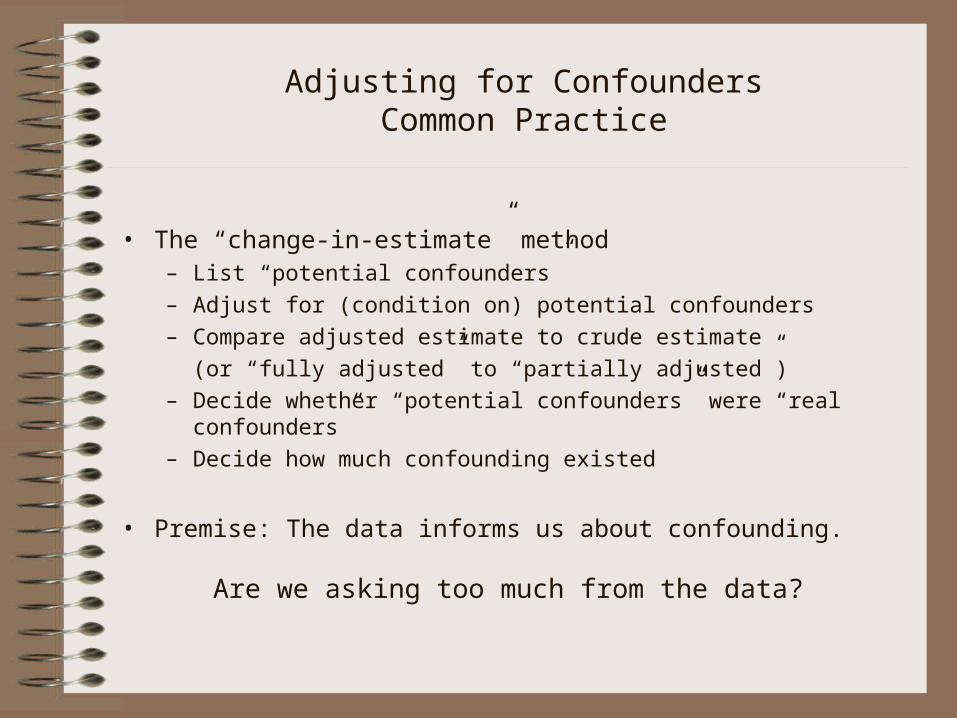
• The “change-in-estimate” method– List “potential confounders”
– Adjust for (condition on) potential confounders
– Compare adjusted estimate to crude estimate
(or “fully adjusted” to “partially adjusted”)
– Decide whether “potential confounders” were “real confounders”
– Decide how much confounding existed
• Premise: The data informs us about confounding.
Adjusting for ConfoundersCommon Practice
Are we asking too much from the data?
Adjusting for ConfoundersCommon Practice
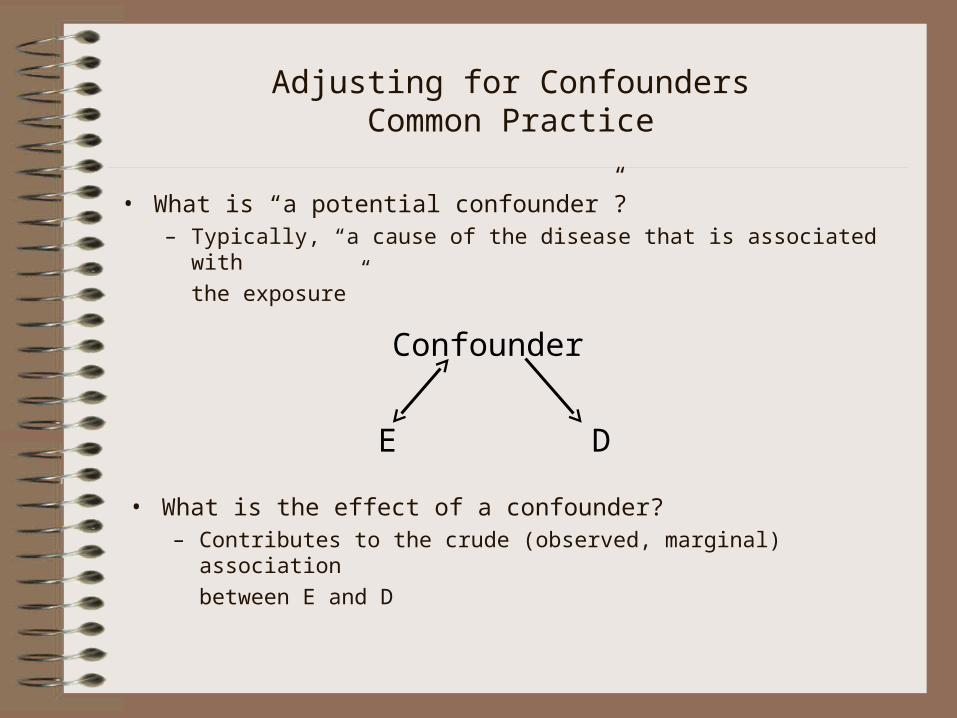
• What is “a potential confounder”?– Typically, “a cause of the disease that is associated with
the exposure”
E D
Confounder
• What is the effect of a confounder?– Contributes to the crude (observed, marginal) association
between E and D

Adjusting for ConfoundersCommon Practice
• Extension to multiple confounders
E D
C1
E D
C4
E D
C2
E D
C3
E D
C5
E D
C6
Adjusting for ConfoundersCommon Practice
Problems
• A sequence of isolated, independent, causal diagrams– but C1, C2, C3, C4, C5,.. might be connected causally
• Unidirectional arrow = a causal direction– but what is the meaning of the bidirectional arrow?
• Even with a single confounder, the “change-in-estimate” method could fail
Adjusting for ConfoundersProblems
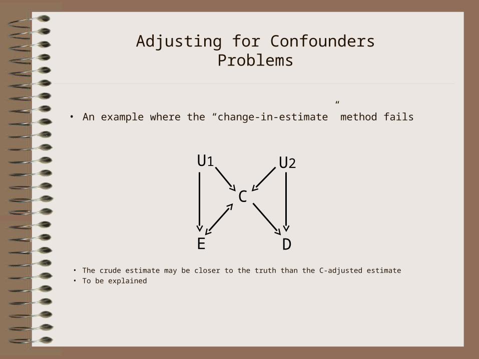
• An example where the “change-in-estimate” method fails
E D
C
U1 U2
• The crude estimate may be closer to the truth than the C-adjusted estimate• To be explained
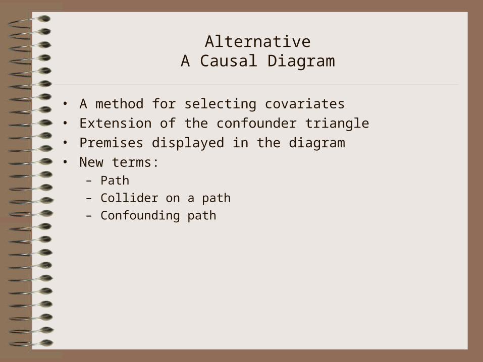
AlternativeA Causal Diagram
• A method for selecting covariates• Extension of the confounder triangle • Premises displayed in the diagram• New terms:
– Path
– Collider on a path
– Confounding path
Selected references
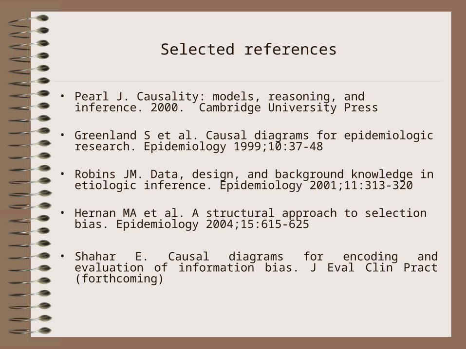
• Pearl J. Causality: models, reasoning, and inference. 2000. Cambridge University Press
• Greenland S et al. Causal diagrams for epidemiologic research. Epidemiology 1999;10:37-48
• Robins JM. Data, design, and background knowledge in etiologic inference. Epidemiology 2001;11:313-320
• Hernan MA et al. A structural approach to selection bias. Epidemiology 2004;15:615-625
• Shahar E. Causal diagrams for encoding and evaluation of information bias. J Eval Clin Pract (forthcoming)
A Causal Diagram Notation and Terms
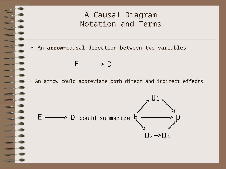
• An arrow=causal direction between two variables
E D
• An arrow could abbreviate both direct and indirect effects
E D could summarize E D
U2 U3
U1
A Causal Diagram Notation and Terms
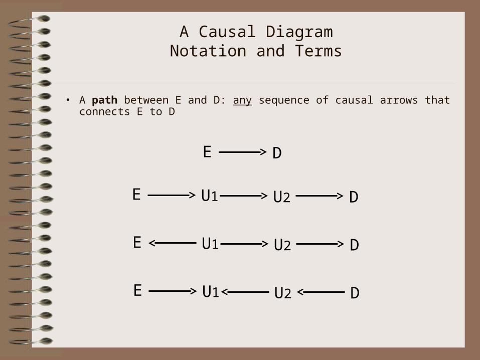
• A path between E and D: any sequence of causal arrows that connects E to D
E D
E U1 U2 D
E U1 U2 D
E U1 U2 D

A Causal Diagram Notation and Terms
• Circularity (self-causation) does not exist: Directed Acyclic Graph
E U1
U2
D
E U1 U2 D
• E and U2 collide at U1
• A collider on the path between E and D
A Causal Diagram Notation and Terms
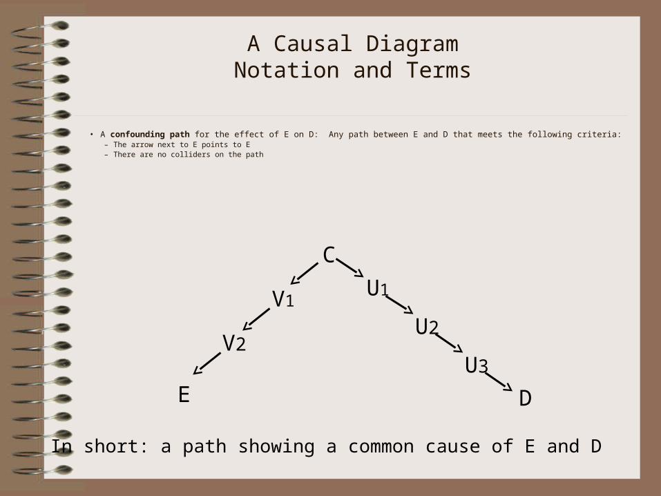
• A confounding path for the effect of E on D: Any path between E and D that meets the following criteria:– The arrow next to E points to E– There are no colliders on the path
E D
C
U1
U2
U3
V1
V2
In short: a path showing a common cause of E and D
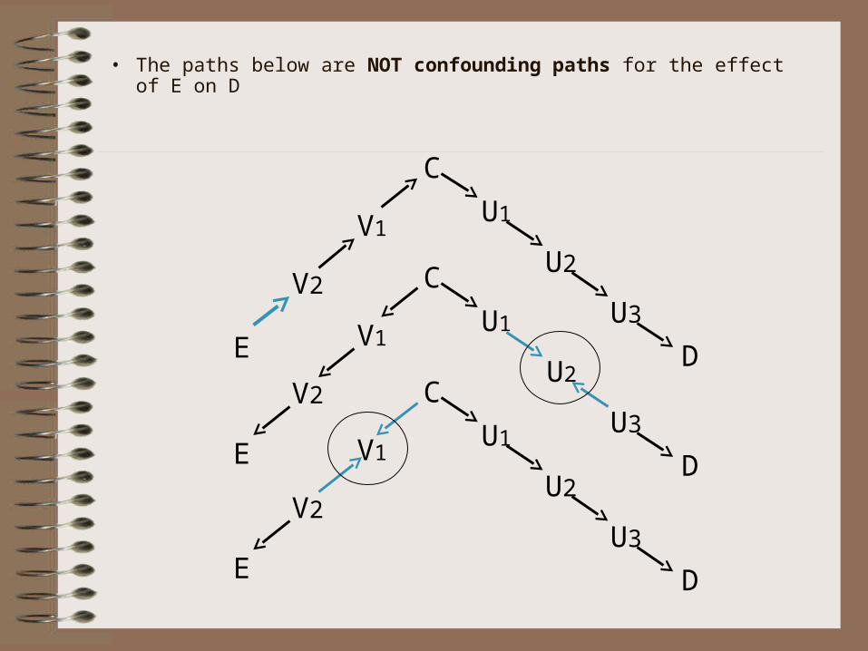
• The paths below are NOT confounding paths for the effect of E on D
E D
C
U1
U2
U3
V1
V2
E D
C
U1
U3
V1
V2U2
V1
E D
C
U1
U2
U3V2
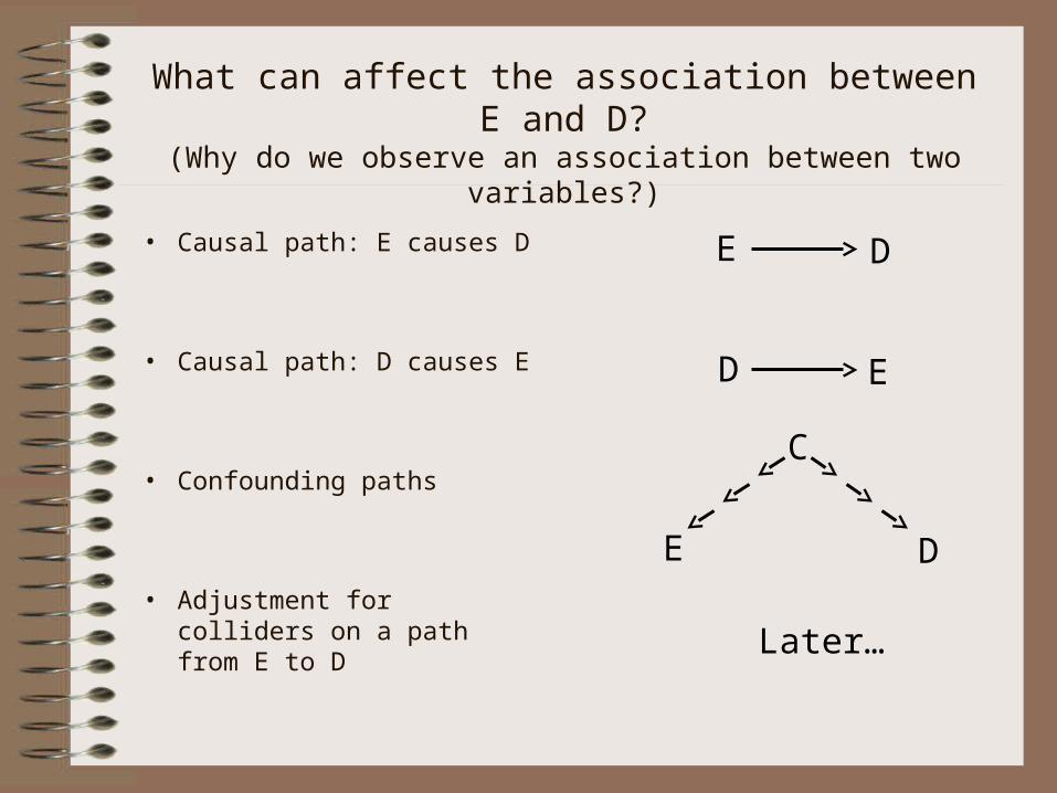
What can affect the association between E and D?(Why do we observe an association between two variables?)
• Causal path: E causes D
• Causal path: D causes E
• Confounding paths
• Adjustment for colliders on a path from E to D
E D
D E
E D
C
Later…

Why does a confounding path affect the crude (marginal) association between E and D?
Intuitively:• Association= being able to “guess” the value of one variable (D)
from the value of another (E)• ED allows us to guess D from E (and E from D)• A confounding path allows for sequential guesses along the
path
E D
U1
U2
U3
V1
V2
C

How can we block a confounding path between E and D?
• Condition on a variable on the path (on any variable)• Methods for conditioning
– Restriction– Stratification– Regression
E D
U1
U2
U3
V1
V2
C
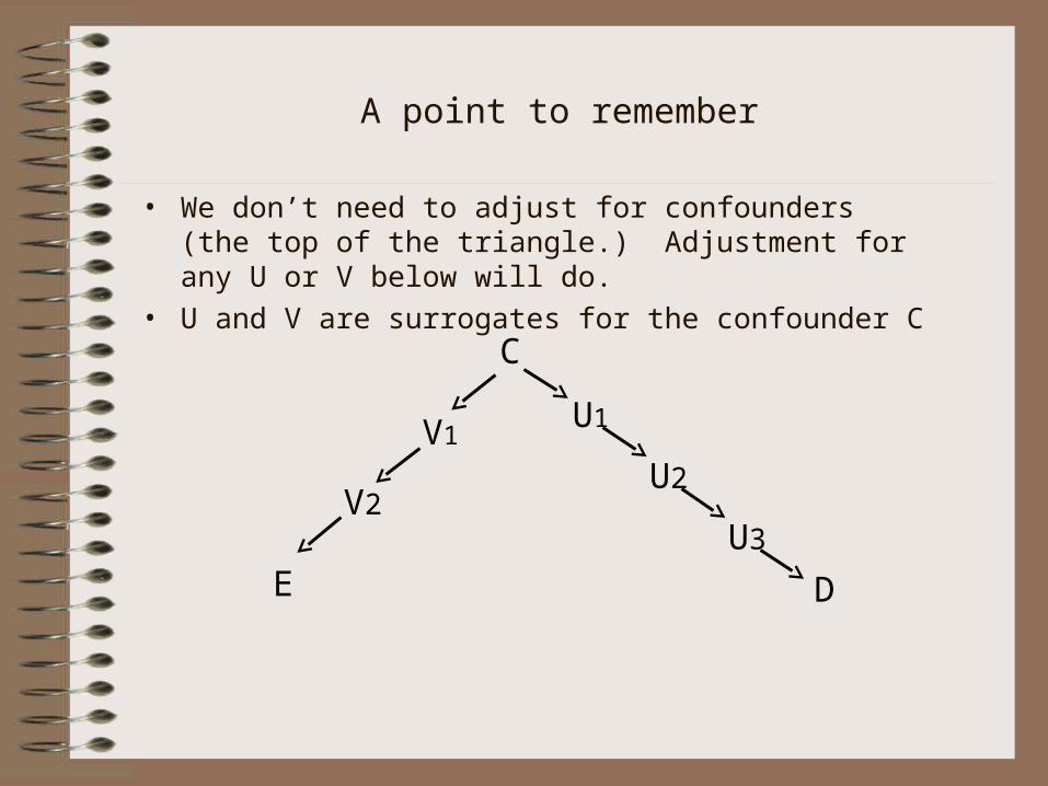
A point to remember
• We don’t need to adjust for confounders (the top of the triangle.) Adjustment for any U or V below will do.
• U and V are surrogates for the confounder C
E D
U1
U2
U3
V1
V2
C
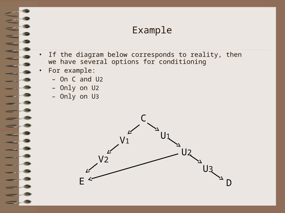
Example
• If the diagram below corresponds to reality, then we have several options for conditioning
• For example: – On C and U2 – Only on U2
– Only on U3
E D
U1
U2
U3
V1
V2
C
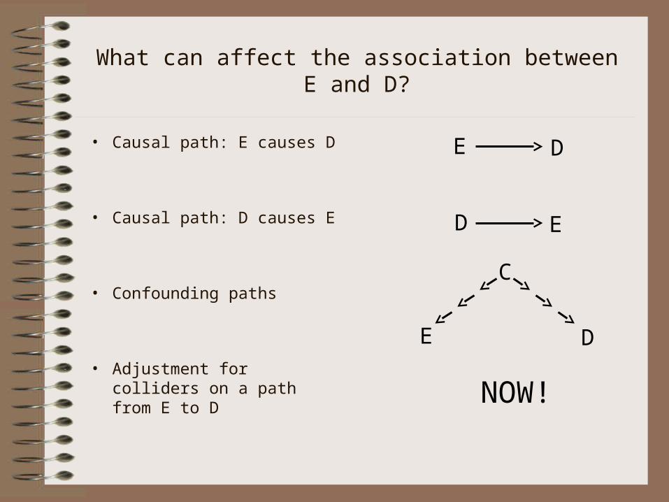
What can affect the association between E and D?
• Causal path: E causes D
• Causal path: D causes E
• Confounding paths
• Adjustment for colliders on a path from E to D
E D
D E
E D
C
NOW!
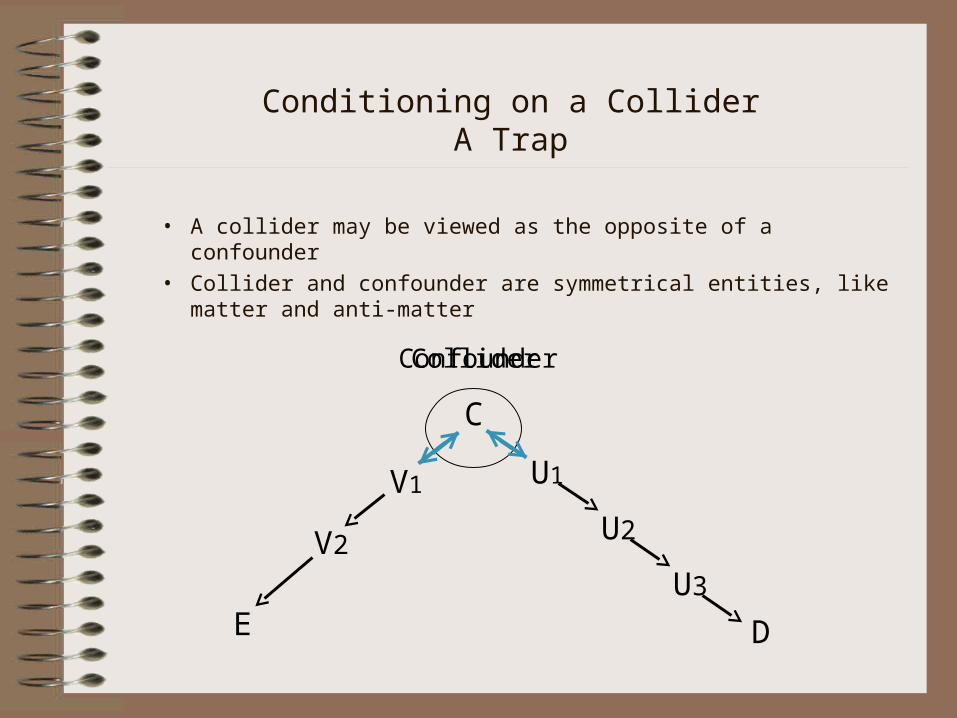
Conditioning on a ColliderA Trap
• A collider may be viewed as the opposite of a confounder• Collider and confounder are symmetrical entities, like
matter and anti-matter
E D
U1
U2
U3
V1
V2
C
ColliderConfounder
Conditioning on a ColliderA Trap
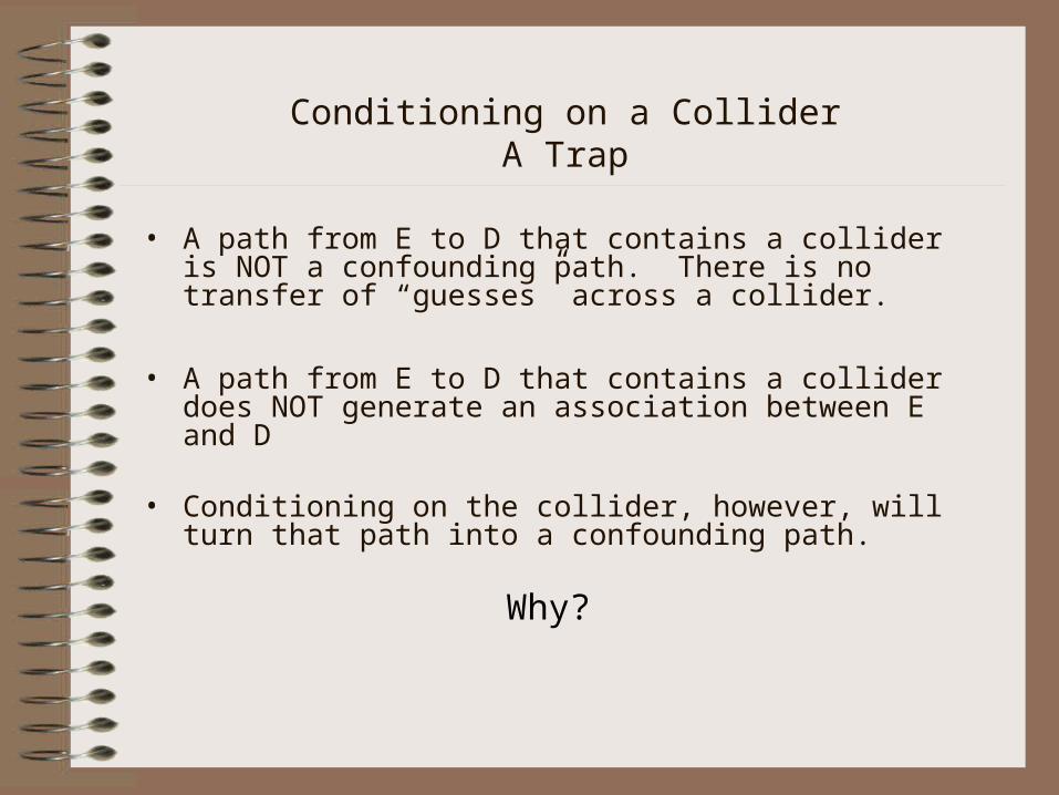
• A path from E to D that contains a collider is NOT a confounding path. There is no transfer of “guesses” across a collider.
• A path from E to D that contains a collider does NOT generate an association between E and D
• Conditioning on the collider, however, will turn that path into a confounding path.
Why?
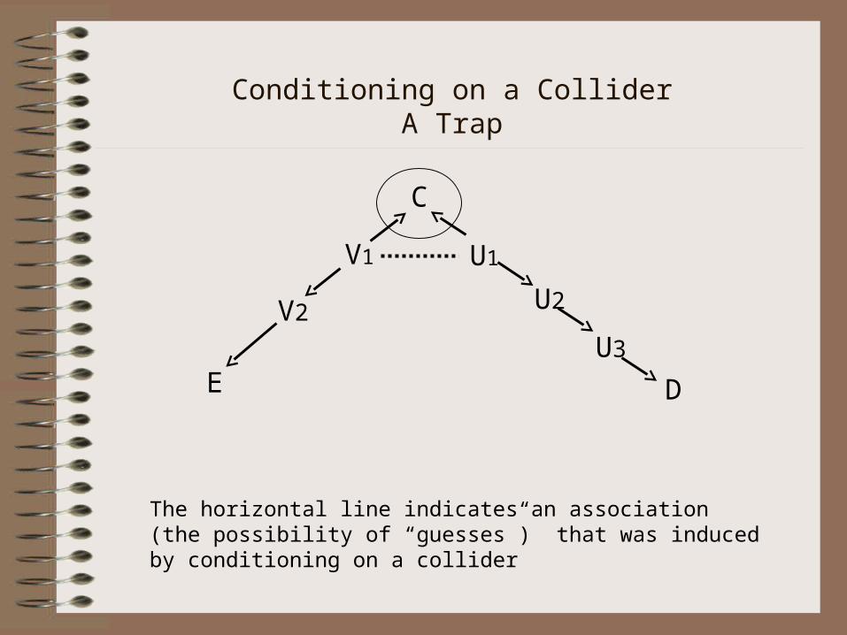
Conditioning on a ColliderA Trap
The horizontal line indicates an association (the possibility of “guesses”) that was induced by conditioning on a collider
E D
U1
U2
U3
V1
V2
C
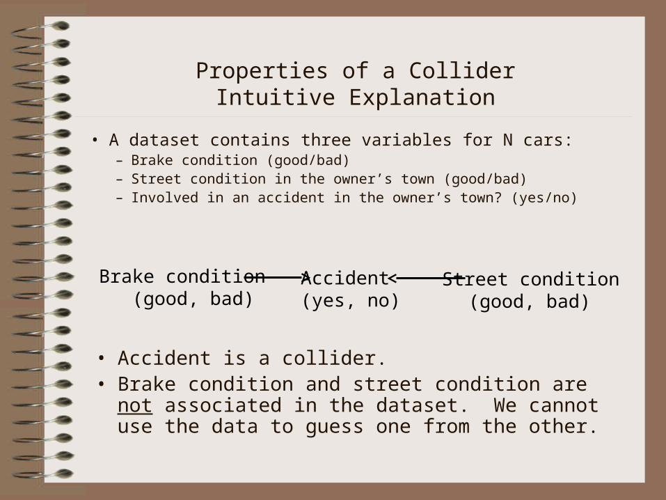
Properties of a ColliderIntuitive Explanation
Brake condition (good, bad)
Street condition (good, bad)
Accident(yes, no)
• A dataset contains three variables for N cars:– Brake condition (good/bad)– Street condition in the owner’s town (good/bad)– Involved in an accident in the owner’s town? (yes/no)
• Accident is a collider. • Brake condition and street condition are not
associated in the dataset. We cannot use the data to guess one from the other.
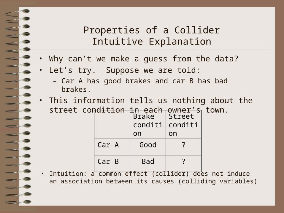
Properties of a ColliderIntuitive Explanation
• Why can’t we make a guess from the data?• Let’s try. Suppose we are told:
– Car A has good brakes and car B has bad brakes.
• This information tells us nothing about the street condition in each owner’s town.
Brake condition
Street condition
Car A Good ?
Car B Bad ?
• Intuition: a common effect (collider) does not induce an association between its causes (colliding variables)
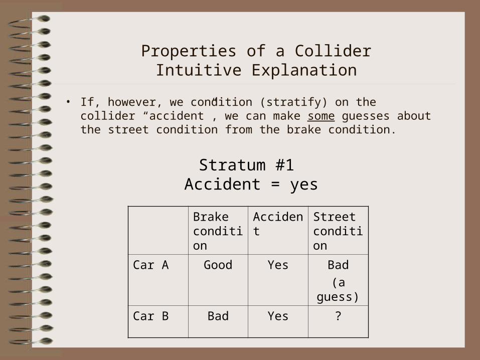
Properties of a ColliderIntuitive Explanation
• If, however, we condition (stratify) on the collider “accident”, we can make some guesses about the street condition from the brake condition.
Brake condition
Accident Street condition
Car A Good Yes Bad
(a guess)
Car B Bad Yes ?
Stratum #1 Accident = yes
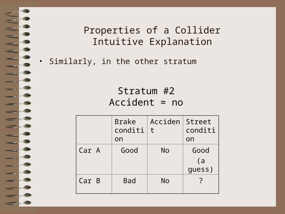
Properties of a ColliderIntuitive Explanation
• Similarly, in the other stratum
Brake condition
Accident Street condition
Car A Good No Good
(a guess)
Car B Bad No ?
Stratum #2Accident = no

Properties of a Collider
In summary:• Conditioning on a collider creates an association between the
colliding variables and, therefore, may open a confounding path
E D
C
U1 U2
Before conditioning on C After conditioning on C
E D
C
U1 U2

Derivations
• The “change-in-estimate” method could fail if we condition on colliders, and thereby open confounding paths
• To (rationally) select covariates for adjustment, we must commit to a causal diagram (premises)
(But we often say that we don’t know and can’t commit, and hope that the change-in-estimate method will work.)
Causal inference, like all scientific inference, is conditional on premises (which may be false)—not on ignorance
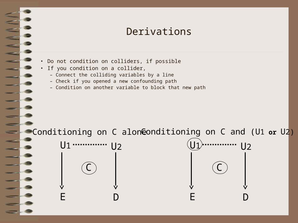
Derivations
• Do not condition on colliders, if possible• If you condition on a collider,
– Connect the colliding variables by a line– Check if you opened a new confounding path– Condition on another variable to block that new path
E D
C
U1 U2
E D
C
U1 U2
Conditioning on C alone Conditioning on C and (U1 or U2)

Practical advice
• Study one exposure at a time
• A model that may be good for exposure A might not be good for exposure B (even if B is in the model)
• Never adjust for an effect of the exposure
• Never adjust for an effect of the disease
• Never select covariates by stepwise regression
• Never look at p-values to decide on confounding• (actually, never look at p-values…)
Extension to other problems of causal inquiry
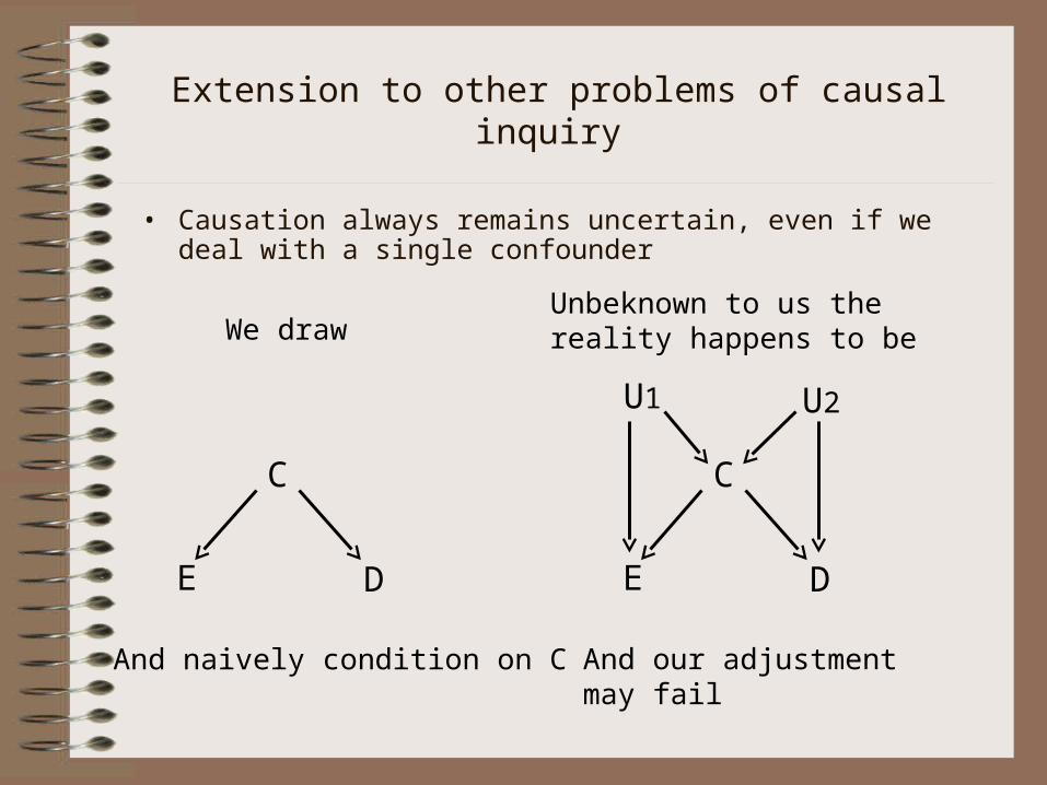
• Causation always remains uncertain, even if we deal with a single confounder
E D
C
We draw
And naively condition on C
E D
C
U1 U2
Unbeknown to us thereality happens to be
And our adjustmentmay fail
Extension to other problems of causal inquiry
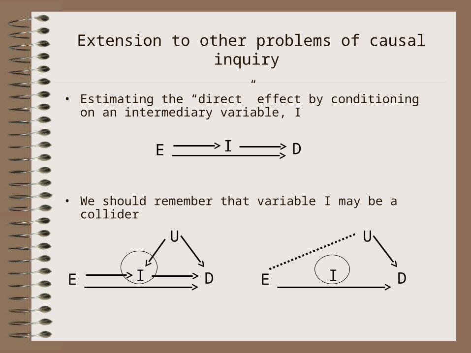
• Estimating the “direct” effect by conditioning on an intermediary variable, I
E I D
• We should remember that variable I may be a collider
E I D
U
E I D
U
Extension to other problems of causal inquiry
• Causal diagrams explain the mechanism of selection bias
• Example:
What happens if we estimate the effect of marital status on dementia in a sample of nursing home residents?
Assume: no effectboth variables affect “place of residence” (home, or nursing home)

Extension to other problems of causal inquiry
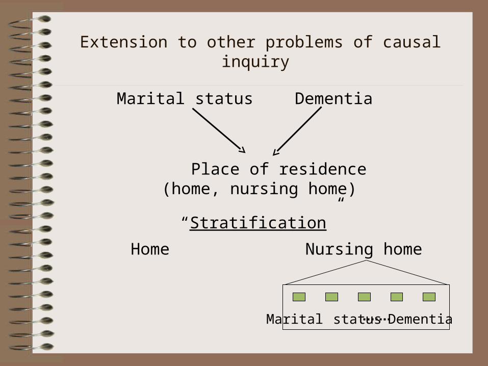
Marital status Dementia
Place of residence(home, nursing home)
• By studying a sample of nursing home residents, we are conditioning on a collider (on a “sampling collider”) and might create an association between marital status and dementia in that stratum
Extension to other problems of causal inquiry
Marital status Dementia
Place of residence(home, nursing home)
Marital status Dementia
Nursing home
“Stratification”
Home

Extensions: control selection bias(Source: Hernan et al, Epidemiology 2004)
S (0,1) Selection into a case-control sample S=1
DS because disease status affectsselection. Diseased members of thecohort are over-sampled (cases) relative to non-diseased (controls)
DE Source cohort: no effectEstrogen MI
Suppose: F is hip fracture
F
E D
S (0,1)
Estrogen MI
Suppose: EF
Suppose: Controls preferentiallyselected from women with hip fracture
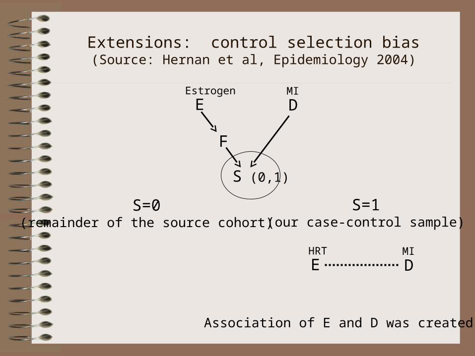
Extensions: control selection bias(Source: Hernan et al, Epidemiology 2004)
E D
S (0,1)
Estrogen MI
F
S=1(our case-control sample)
S=0(remainder of the source cohort)
E DHRT MI
Association of E and D was created
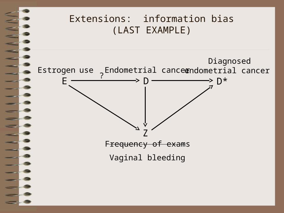
Extensions: information bias(LAST EXAMPLE)
E DEstrogen use Endometrial cancer
D*
Diagnosed endometrial cancer
?
ZFrequency of exams
Vaginal bleeding
Summary Points
• The “change-in-estimate” method could fail if we condition on colliders, and thereby open confounding paths
• The theory of causal diagrams extends the idea of a confounder to the multi-confounder case
• Unification of confounding bias, selection bias, and information bias under a single theoretical framework

• “Back-door algorithm”• Sufficient set for adjustment• Minimally sufficient set• Differential losses to follow-up• Time-dependent confounders• Interpretation of hazard ratios• Conditioning on a common effect always induced an
association between its causes, but this association could be restricted to some levels of the common effect
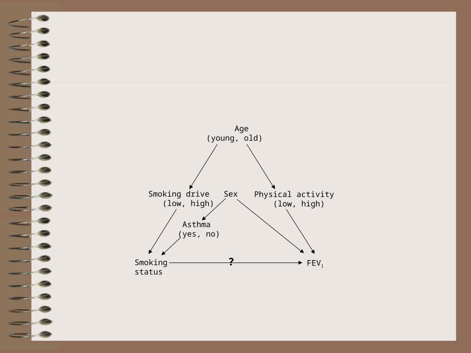
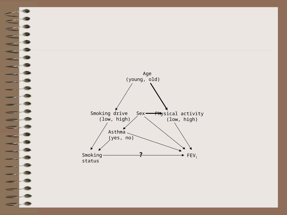
Smokingstatus
FEV1
Sex
?
Age (young, old)
Smoking drive (low, high)
Physical activity (low, high)
Asthma (yes, no)
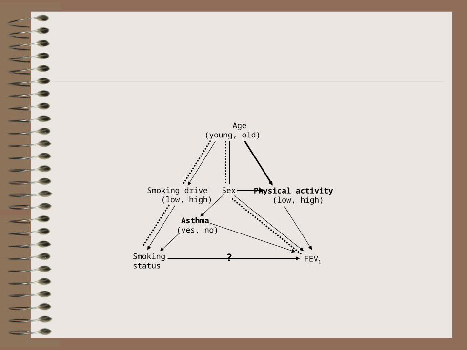
Smokingstatus
FEV1
Sex
?
Age (young, old)
Smoking drive (low, high)
Physical activity (low, high)
Asthma (yes, no)
Smokingstatus
FEV1
Sex
?
Age (young, old)
Smoking drive (low, high)
Physical activity (low, high)
Asthma (yes, no)
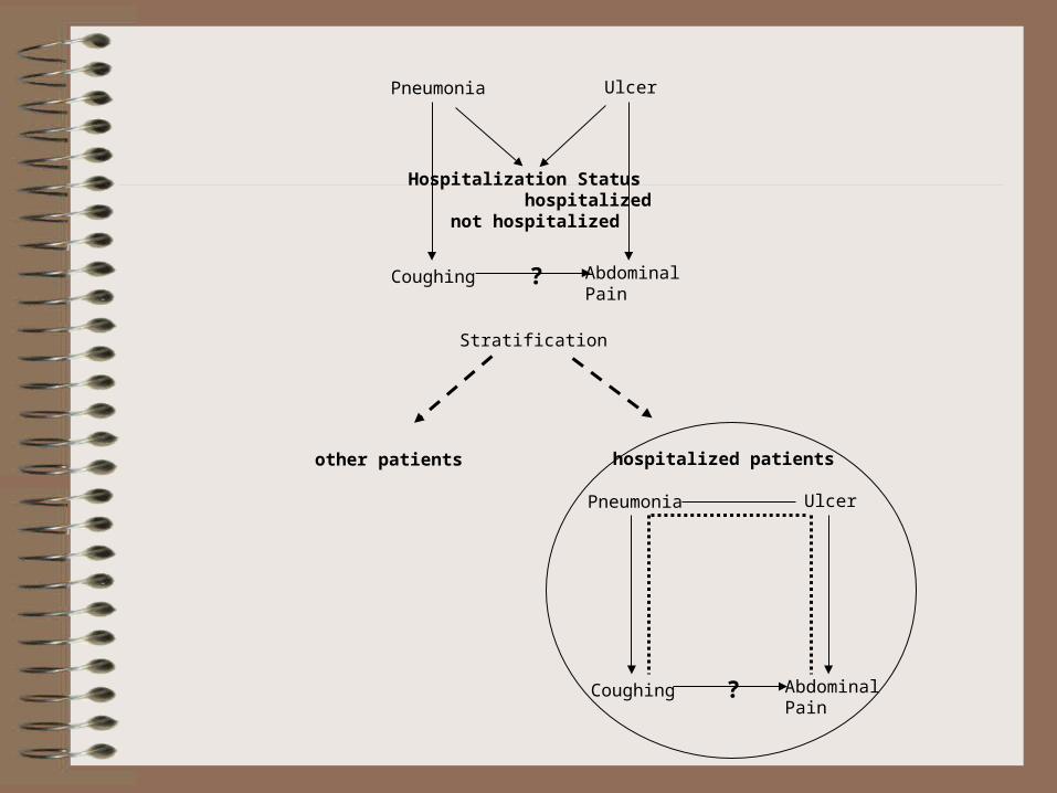
Hospitalization Status hospitalized not hospitalized
Pneumonia Ulcer
Coughing Abdominal Pain
Pneumonia Ulcer
Coughing Abdominal Pain
Stratification
hospitalized patientsother patients
?
?
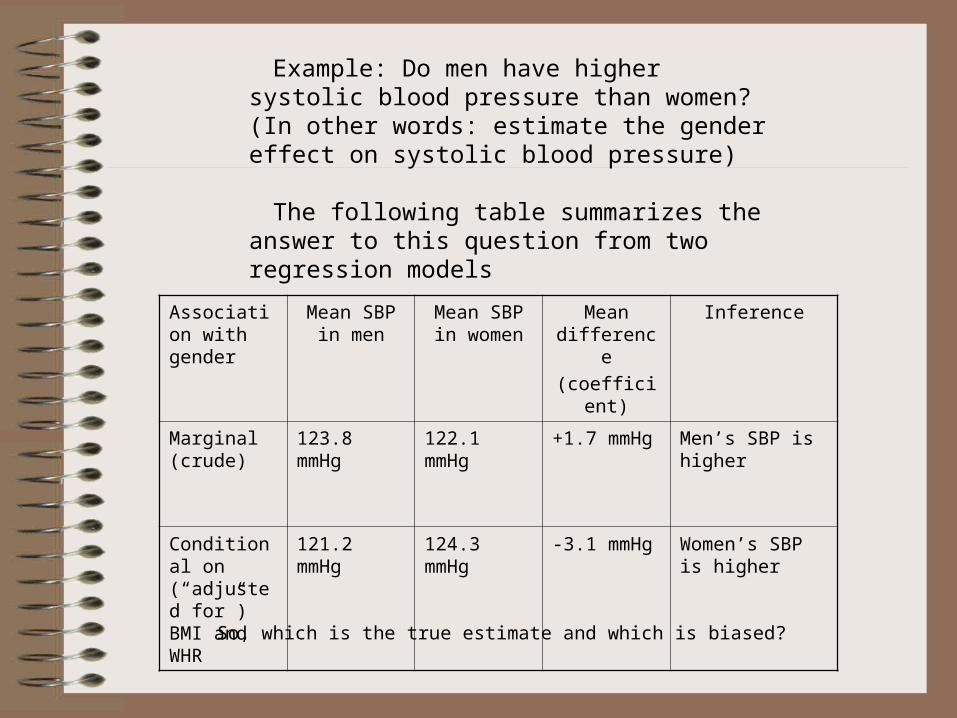
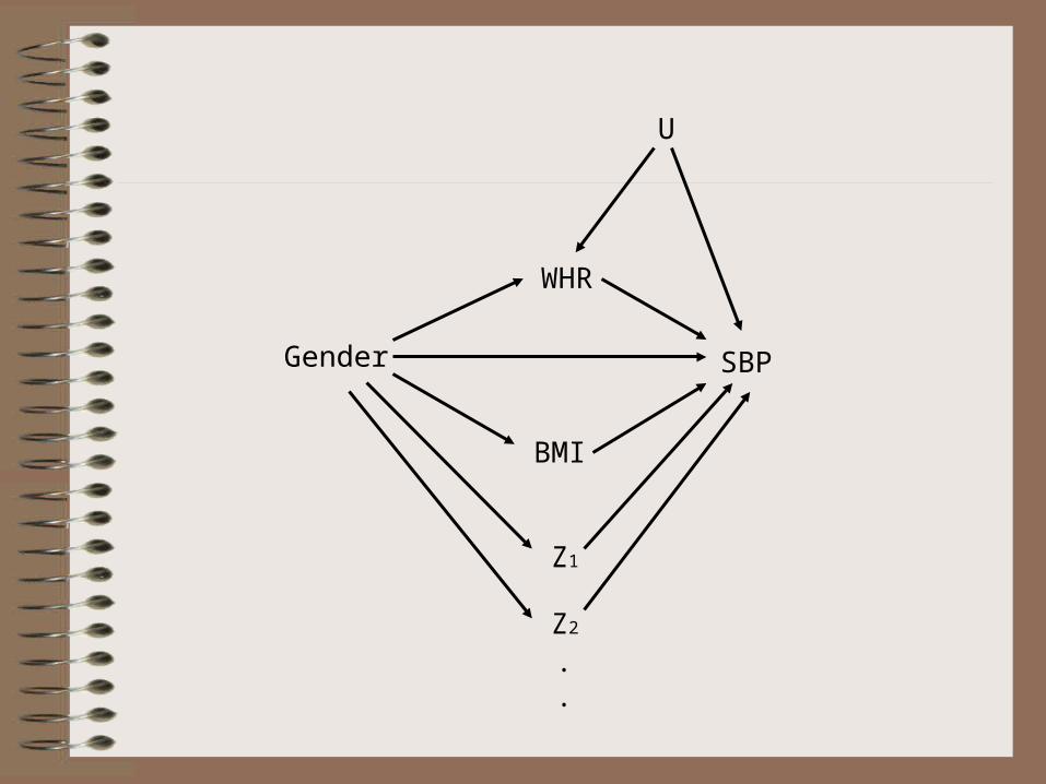
Example: Do men have higher systolic blood pressure than women? (In other words: estimate the gender effect on systolic blood pressure)
The following table summarizes the answer to this question from two regression models
So, which is the true estimate and which is biased?
Association with gender
Mean SBP in men
Mean SBP in women
Mean difference
(coefficient)
Inference
Marginal (crude)
123.8 mmHg 122.1 mmHg +1.7 mmHg Men’s SBP is higher
Conditional on (“adjusted for”) BMI and WHR
121.2 mmHg 124.3 mmHg -3.1 mmHg Women’s SBP is higher

Gender SBP
WHR
BMI
Z1
Z2
.
.
Gender SBP
WHR
BMI
Z1
Z2
.
.
U

Gender SBP
WHR
BMI
Z1
Z2
.
.
U