Appendix D Progress towards Australia’s emissions reduction goalsAustralia faces a major task to meet the Authority’s recommended emissions reduction goals. Australia’s emissions are projected to rise, underpinned by population and economic growth. Strong policies will be needed to turn this around and drive the transition to a lower emissions economy.

Australia has significant emissions reduction opportunities in the domestic economy. A price incentive could drive substantial emissions reductions, particularly in electricity generation, fugitive emissions and industrial processes. The minimum 5 per cent emissions reduction target could be achieved solely through domestic emissions reductions, provided a strong and effective suite of policies is in place. The Authority’s recommended 2020 target could be met by complementing domestic emissions reductions with international units. Depending on the policies implemented, the required reduction in emissions could be achieved for relatively small economic cost, and while maintaining economic growth and rising incomes.

Cost-effective and complementary policies must be put in place now and sustained to support the development of a lower emissions economy in the decades beyond 2020. Most of Australia’s emissions come from long-lived equipment, buildings and vehicles, which will take time to change. In many cases, policies will not influence the majority of stock until 2030.

The most important sector for potential emissions reductions is electricity. It has the largest share of Australia’s emissions and its emissions are projected to grow strongly without price incentives or additional policies. In scenarios with a price incentive, however, the electricity sector is projected to account for the largest share of emissions reductions. The RET is another important driver, as is action to increase the uptake of energy efficiency.

Further emissions reductions are also available. Light vehicle efficiency standards have delivered cost-effective reductions in other markets; their use in Australia warrants investigation. In the near term, targeted policies should be implemented to increase the uptake of energy efficiency more broadly. Depending on policy incentives, in the longer term the land sector could also offer large emissions reductions.

Appendix D1 Evaluating progress

As outlined in Chapter 1, the Clean Energy Act requires the Authority to review Australia’s progress towards its medium- and long-term emissions reduction goals. Appendix D, together with chapters 6, 11 and 12, fulfils this legislative requirement.

Appendix D1 sets out the purpose, scope and approach to the review of progress. Appendix D2 highlights the outlook for emissions from the Australian economy as a whole. Appendices D3–D10 outline the outlook for changes in emissions from each sector, expanding on the discussion in Chapter 11.

D1.1 Purpose and scope of the Review

To meet its emissions reduction goals, Australia has implemented a range of policy measures, as discussed in Chapter 5. This Review assesses how Australia is tracking towards its emissions reduction goals, providing important feedback to government on changes taking place in the economy in response to these policy measures and other factors.

This Review focuses on the outlook for emissions across the economy under several scenarios and also considers the outlook for changes in emissions in different sectors. The approach is designed to assess if and how Australia might achieve its emissions reduction targets. Considering the projected outcomes in each sector helps to identify opportunities to transition to a lower emissions economy, and determine the efficiency of policy measures and their impact on different sectors.

The Authority has based its Review on the four scenarios described in Chapter 10 and Appendix F (no price, low, medium and high scenarios). The Authority has also drawn on additional modelling, published material and expert input to provide a broader review of possible future outcomes.

D1.2 Stakeholder views on the Authority’s Review

Some stakeholder submissions to the Issues Paper for this Review raised concerns that assessing progress by referring to developments in each sector may imply sector-specific emissions targets or development pathways. There were concerns such an approach could compromise Australia’s broad-based strategy to reducing emissions.

The Authority does not recommend binding sector-specific objectives or prescribe pathways, technologies or activities to reach Australia’s emissions reduction goals. Rather, the Review synthesises information from multiple sources to better understand possible paths towards emissions reductions and the factors (‘contributors’) likely to lead to

significant changes in emissions. The Authority’s analysis considers the likelihood and timing of potential outcomes. This can help identify if Australia is on track to meet its broader national emissions reduction goals, and how those goals may be met.

Some stakeholders called for a focus on policy as a driver of changes in emissions. The Authority has not estimated the change in emissions from any specific policy or legislation, though it has considered the potential of general policy options. The emissions reduction potential of specific policy is generally determined as part of the process of developing or evaluating regulatory instruments. Instead, the Review seeks to identify drivers of change in emissions; across successive annual progress reviews this could identify policies with a significant effect on activity and emissions.

The Review does not explicitly assess the cost-effectiveness of policies, but does identify opportunities for changes in technology or behaviour to increase the uptake of cost-effective emissions reductions in future, and policy options that warrant further investigation. The Authority focuses on the most substantive contributors and drivers of emissions outcomes. While policy is relevant, macroeconomic and other drivers are also important.

D1.3 Framework for analysing progress

The Authority’s analytic framework for assessing progress considers:

Australia’s domestic emissions levels and emissions intensity, recent trends and projections

historical and projected sectoral emissions outcomes, the key contributors to those outcomes, and the underlying economic, policy and technological drivers.

D1.4 Considering activity and supply intensity

In this Review, emissions are disaggregated into activity levels and emissions intensity to give a more comprehensive picture of Australia’s progress. For example, emissions in the electricity sector are affected by both the amount of electricity generated (the activity level) and the emissions intensity of generation.

It is important to highlight the extent to which emissions levels, both historical and projected, reflect changing levels of activity compared with the emissions intensity of that activity. This distinction helps illustrate

the projected strong growth in activity for most parts of the economy. It is also useful in informing policy, since different policy instruments often focus on either decreasing emissions intensity, or changing demand or activity.

D1.5 Reviewing progress economy-wide and by sector

The economy-wide analysis considers the relative contribution of different sectors to changes in domestic emissions, based on taking up emissions reduction opportunities to a certain marginal cost.

The sectoral analysis of progress (appendices D3–D10) identifies potential emissions outcomes in absolute terms and in terms of activity levels and emissions intensity. Sectoral analyses are designed to, over time:

identify the greatest contributors to changes in sector emissions, including those that affect levels of activity and the emissions intensity of the sector’s activity

track the main contributors to projected emissions outcomes and the drivers that underpin them

allow comparison between modelled and realised sectoral outcomes, helping to anticipate when contributors or drivers will persist, subside or recur.

The Authority has adopted the same approach to define sectors and organise its sector-level reporting as is used in Australia’s National Greenhouse Gas Inventory—electricity generation, transport, direct combustion, fugitives, industrial processes, agriculture, LULUCF and waste.

The Authority also uses complementary analysis of emissions attributed to end-use categories, such as buildings, where it provides additional information or helps consider opportunities for, or barriers to, cost-effective emissions reductions.

D1.6 Assessing emissions changes against a fixed baseline

This appendix does not focus on emissions reduction relative to a concept of BAU (or ‘no price’ scenario). BAU projections depend on the broader economic and policy context at a point in time and, as such, fail to provide a stable and robust basis for tracking progress towards fixed

long-term targets. Instead, the Authority uses 2000 as the base year against which to assess changes in emissions. This approach:

is consistent with the expression of Australia’s emissions reduction targets

avoids the use of a BAU reference, supporting longer term comparison of Australia’s progress that remains relevant as the economic conditions and legislative framework change over time

is easily rebased to alternative reference years, if required.

Australia’s total emissions in 2000 were 586 Mt CO2-e.

In contrast to Appendix D, Chapter 11 most often compares emissions projections relative to a counterfactual ‘no price’ scenario.

D1.7 Synthesising data sources and quantifying emissions

This Review uses historical and projected emissions for the period 1990–2030 from Treasury and DIICCSRTE modelling (2013). In that report:

the data incorporates National Greenhouse Gas Inventory data for the 2010–11 inventory year and preliminary emissions estimates for 2011–12 and 2012–13

emissions for 2012 are based on preliminary inventory data and modelled estimates available at the time Treasury and DIICCSRTE modelling was undertaken (March 2013). They do not reflect 2012 or 2013 emissions reported in the June 2013 Quarterly Update of Australia’s National Greenhouse Gas Inventory, released in December 2013. The June 2013 Quarterly Update is the source of Australia’s estimated carryover from the first commitment period of the Kyoto Protocol. Revisions incorporated in the June 2013 Quarterly Update revise estimated 2012 emissions, but have almost no effect on the rate of growth in emissions between 2011–12 and 2012–13

the data for emissions for the period 2013–2030 are modelled estimates (see Appendix C)

historical emissions for the LULUCF sector for the period 1990–2012 are based on an estimate of emissions consistent with the new accounting rules (Article 3.4) agreed for the second commitment period of the Kyoto Protocol

all emissions data has been converted to CO2-e using global warming potentials from the IPCC Fourth Assessment Report. Historical emissions for LULUCF for the period 1990 to 2012 have been adjusted to be consistent with the new accounting rules agreed for the second commitment period of the Kyoto Protocol. This means historical and projected emissions data throughout the report is directly comparable.

All data in this report is for the financial year ending 30 June unless otherwise indicated. For example, data reported for 2013 is for the financial year 2012–13. All dollar amounts (prices and costs) reported in this appendix are 2012 Australian dollars, unless otherwise stated.

In December 2013, the National Greenhouse Gas Inventory was updated for the 2012–13 year, with refinements to earlier years’ emissions levels. For consistency with the modelled scenarios, Appendix D retains the historical emissions data on which the Treasury and DIICCSRTE modelling is based.

Modelling from the Treasury and DIICCSRTE has formed the core data set analysed in this Review, including four core scenarios—one without a carbon price, and three different price levels (Box D.1). The electricity, transport and agriculture sectors were modelled separately in greater detail, and scenarios and sensitivities from these models are also included.

Box D.1: Modelling scenarios used to track emissions progress

No price scenario—assumes there is no carbon price and no CFI. This scenario includes emissions reductions from pre-existing measures such as energy efficiency measures and the RET.

Low scenario—additionally assumes the carbon price and CFI are in place. The carbon price is fixed for two years, then moves to a flexible price. The flexible price begins at $5.49/t CO2-e in 2015, and grows at 4 per cent per year in real terms to reach $6.31 in 2020. The price then follows a linear transition to $54.48 in 2030.

Medium scenario—assumes the fixed price for two years, then a flexible price beginning at $5.49/t CO2-e in 2015, and following a linear transition to $30.14 in 2020. From 2021, the price follows the international price from the medium global action scenario, which grows at 4 per cent per year in real terms in US dollars.

High scenario—assumes the fixed price for two years, then a flexible price beginning at $5.49/t CO2-e in 2015, and following a linear transition

to $73.44 in 2020. From 2021, the price follows the international price from the ambitious global action scenario, which grows at 4 per cent per year in real terms in US dollars.

The effective carbon price faced by liable entities is lower than the modelled price in the low, medium and high scenarios. Kyoto units such as CERs currently trade at prices well below the prices used in these scenarios and the modelling assumes there is a price difference between CERs and ACUs for the period to 2020. The effective carbon price faced by liable entities is a weighted average of the ACU and CER price, with weights reflecting the CER sub-limit (12.5 per cent of their liability).

Chapter 10 of this Review and Table 3.1 of the Treasury and DIICCSRTE (2013) modelling report provide further details of the scenario assumptions.

It is useful to consider uncertainty when assessing possible future outcomes. Among other things, Australia’s emissions may be higher or lower as a result of changes in the level of global action on climate change, the Australian legislative framework, economic growth, demographic factors and technology costs. The Review notes opportunities, risks and barriers to delivering emissions reductions projected in recent modelling and analysis. The Authority considers the four scenarios described earlier, alongside sensitivity analyses and alternative projections, to explore some important variables.

The Authority acknowledges that modelling presents possible future outcomes based on a particular set of assumptions. This analysis has also drawn on additional published sources and expert input to supplement modelling results and give a broader picture of potential futures. Appendix D explores opportunities for greater emissions reductions than those projected, as well as risks and barriers to realising the emissions outcomes projected by the modelling.

This Review provides a more detailed assessment of the outlook for the electricity and transport sectors than for other parts of the economy. In subsequent progress reviews, similarly detailed consideration of emissions from other sectors could be undertaken, over time building an economy-wide picture of possible paths for reductions in emissions.

D1.8 Selecting contributors and drivers

The Authority analyses progress in terms of contributors and drivers.

D1.8.1 Contributors

Contributors are changes that directly affect the emissions outcomes. They may include factors that affect emissions intensity, such as changes in process, fuels or technology. Generally, a sector’s activity level will be a contributor to its emissions outcomes.

The Authority has focused on contributors to emissions outcomes that are:

projected to deliver a significant proportion of Australia’s changes in emissions by 2050, whether at a point in time or in aggregate (nominally over 5 per cent of domestic emissions changes)

among the top few contributors to emissions reductions, at a point in time or in aggregate, in a sector.

The Authority has also examined other contributors that:

could be deployed broadly across the sector under plausible conditions

are likely to lock in emissions reductions (or increases)

have a relatively long lead time for deployment

offer low-cost emissions reductions

offer significant co-benefits (or disadvantages) outside of their potential emissions impacts

are explicitly identified by sector experts for other reasons.

D1.8.2Drivers

Drivers are the underlying factors that promote or impede contributors, but do not directly affect emissions outcomes. Drivers may include factors such the rate of growth in GNI, relative technology costs, population growth or policy.

The underlying drivers are identified to give a sense of the risks, uncertainties, barriers and opportunities to domestic emissions reduction and, therefore, Australia’s progress in meeting its emissions reduction goals.

D1.8.3Illustrating progress

Appendix D introduces two styles of charts to help describe Australia’s progress towards its emissions reduction goals.

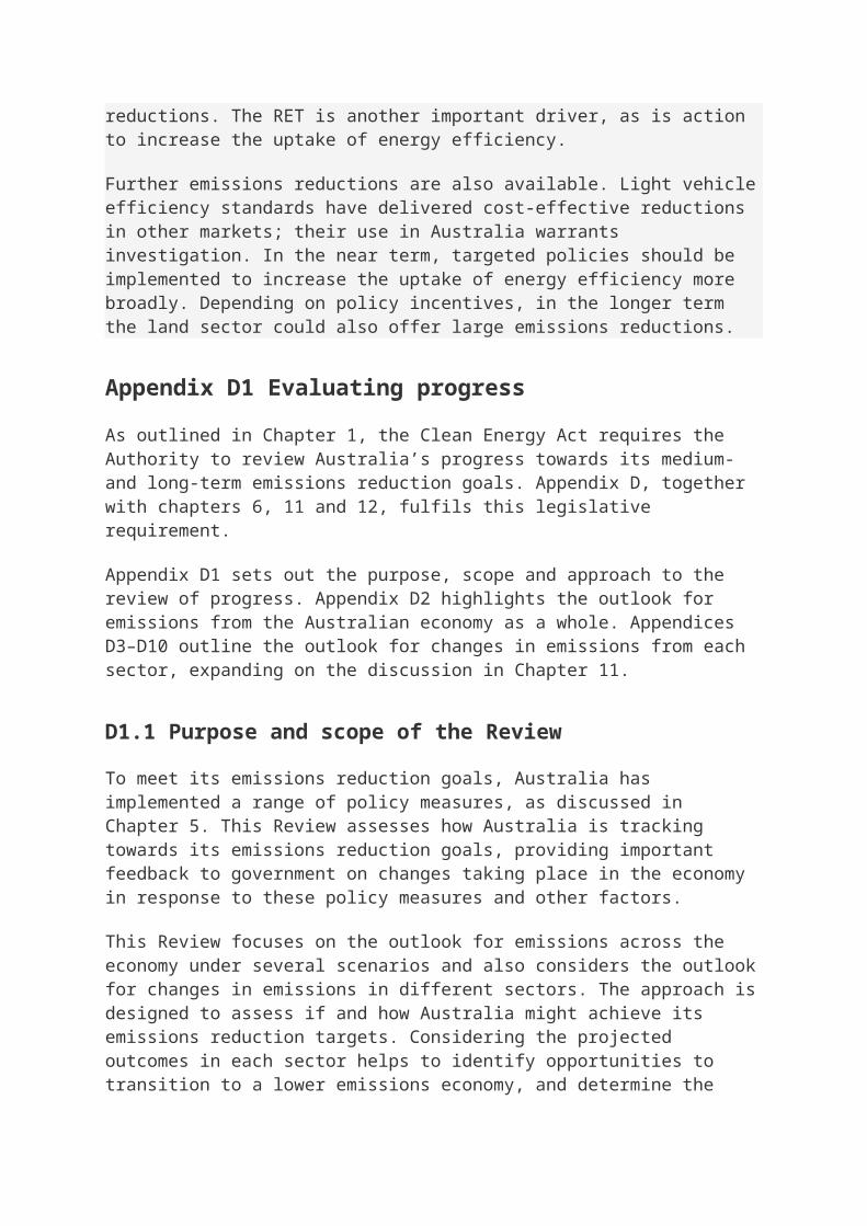
Australia’s emissions are, for the most part, characterised by decreases in emissions intensity offsetting increasing activity. The first chart (Figure D.1) shows changes in emissions intensity against demand-side activity. This highlights whether increasing activity or decreasing supply intensity have the greatest effect on absolute emissions.

The horizontal axis represents total activity levels in the relevant sector. Depending on the sector, activity may be, for example, electricity generated, energy combusted or kilometres travelled. The vertical axis represents the emissions per unit of activity. It is a measure of emissions intensity in the relevant sector. Curved isolines represent absolute emissions levels. The plot(s) on the chart are presented to show the historical and projected changes in activity, emissions intensity and absolute emissions. Date labels indicate the progression of emissions outcomes over time.

Figure D.1: Examples of trends in emissions intensity and activity

 

Source: Climate Change Authority

Figure D.1 shows four plot examples:

Plot A shows a trend of increasing emissions intensity and activity, with corresponding increasing absolute emissions levels.

Plot B shows a trend of stable emissions intensity coupled with activity growth, leading to increasing levels of absolute emissions.

Plot C shows a trend of falling emissions intensity balancing increasing activity levels, leading to stable absolute emissions (following the emissions isoline).

Plot D shows a trend of falling emissions intensity against stable activity levels, leading to a reduction in absolute emissions.

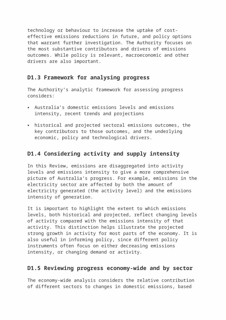
The second chart (Figure D.2) summarises projected emissions outcomes for a given year and the contributors to changes in emissions outcomes, relative to 2000 emissions levels.

Read from left to right, the bars represent the increasing level of price incentive, from the no price scenario to the high scenario, for a given sector.

Each bar is divided into the main contributors to changes in emissions, whether increasing or decreasing emissions, compared to 2000 levels. These contributors may represent changes in activity levels, supply intensity, or the net contribution of a particular subsector or other area of interest.

The net change in emissions—that is, the sum of all the contributors—is represented by the red circles.

Figure D.2: Examples of trends in emissions intensity and activity,

1990–2030

 

Source: Climate Change Authority

Appendix D2 Whole-of-economy

D2.1 Indicators for the Australian economy

As described in Chapter 6, Australia’s domestic emissions have been relatively stable since 2000, despite significant population and economic growth.

Since 2000, Australia’s emissions have increased by 2.5 per cent, driven by increases in emissions across most sectors. Emissions reductions from LULUCF have offset most of the increase from the remainder of the economy.

The Treasury and DIICCSRTE modelling projects that between 2000 and 2020 emissions could rise by 17 per cent in the no price scenario and fall by 6 per cent under the high scenario. The gap widens over time—by 2030, emissions could rise by 37 per cent in the no price scenario and fall by 21 per cent under the high scenario (see Figure D.3). The modelling indicates that the electricity sector will account for the largest emissions reduction of any sector in the low, medium and high scenarios, followed by the fugitives sectors.

Figure D.3: Australia’s emissions, 1990–2030

 

Source: Climate Change Authority calculations using results from Treasury and DIICCSRTE 2013

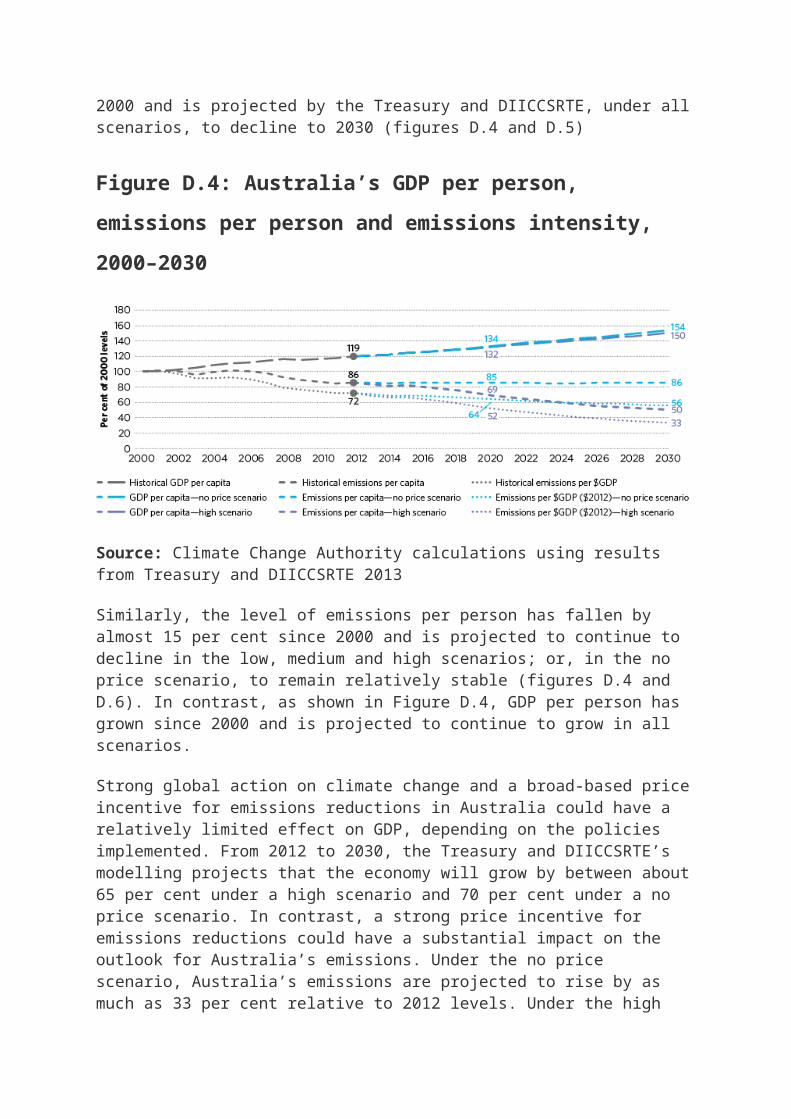
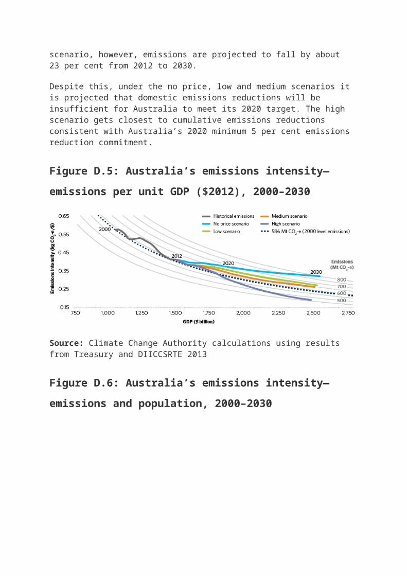
Emissions intensity of the economy, as indicated by the ratio of domestic emissions to GDP, has reduced 28 per cent since 2000 and is projected by the Treasury and DIICCSRTE, under all scenarios, to decline to 2030 (figures D.4 and D.5)

Figure D.4: Australia’s GDP per person, emissions per person and

emissions intensity, 2000–2030

 

Source: Climate Change Authority calculations using results from Treasury and DIICCSRTE 2013

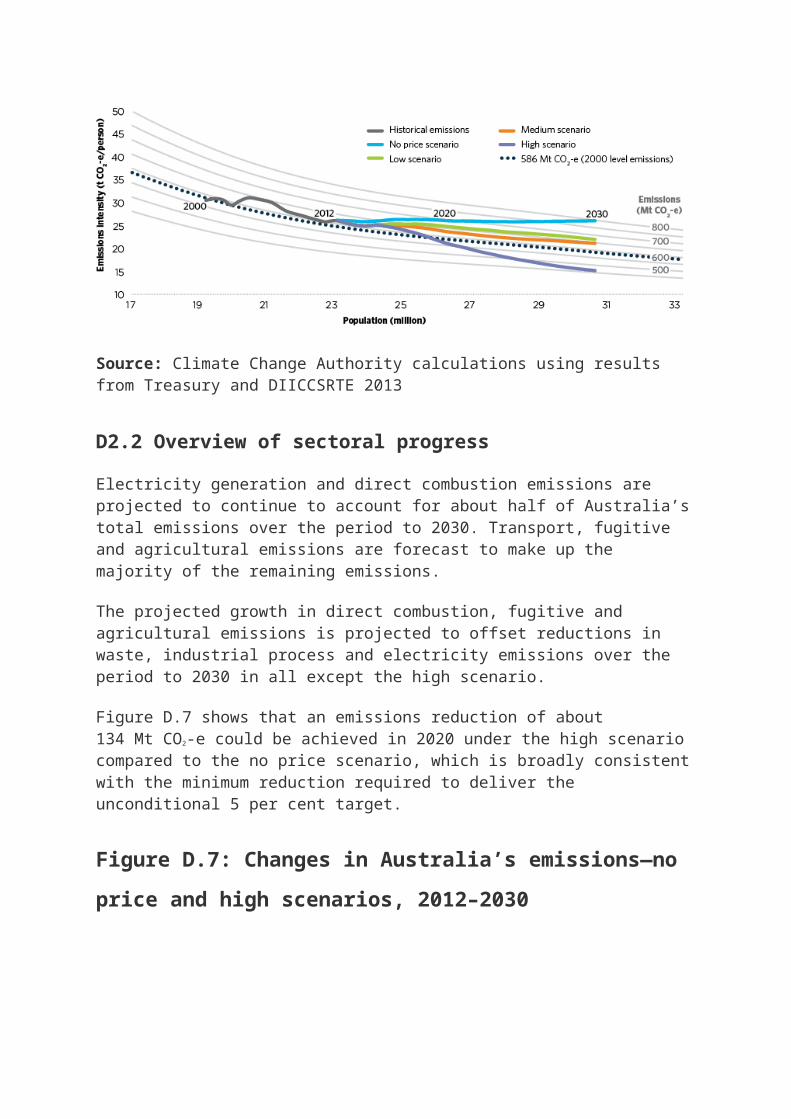
Similarly, the level of emissions per person has fallen by almost 15 per cent since 2000 and is projected to continue to decline in the low, medium and high scenarios; or, in the no price scenario, to remain relatively stable (figures D.4 and D.6). In contrast, as shown in Figure D.4, GDP per person has grown since 2000 and is projected to continue to grow in all scenarios.

Strong global action on climate change and a broad-based price incentive for emissions reductions in Australia could have a relatively limited effect on GDP, depending on the policies implemented. From 2012 to 2030, the Treasury and DIICCSRTE’s modelling projects that the economy will grow by between about 65 per cent under a high scenario and 70 per cent under a no price scenario. In contrast, a strong price incentive for emissions reductions could have a substantial impact on the outlook for Australia’s emissions. Under the no price scenario, Australia’s emissions are projected to rise by as much as 33 per cent relative to 2012 levels. Under the high scenario, however, emissions are projected to fall by about 23 per cent from 2012 to 2030.

Despite this, under the no price, low and medium scenarios it is projected that domestic emissions reductions will be insufficient for Australia to meet its 2020 target. The high scenario gets closest to cumulative emissions reductions consistent with Australia’s 2020 minimum 5 per cent emissions reduction commitment.

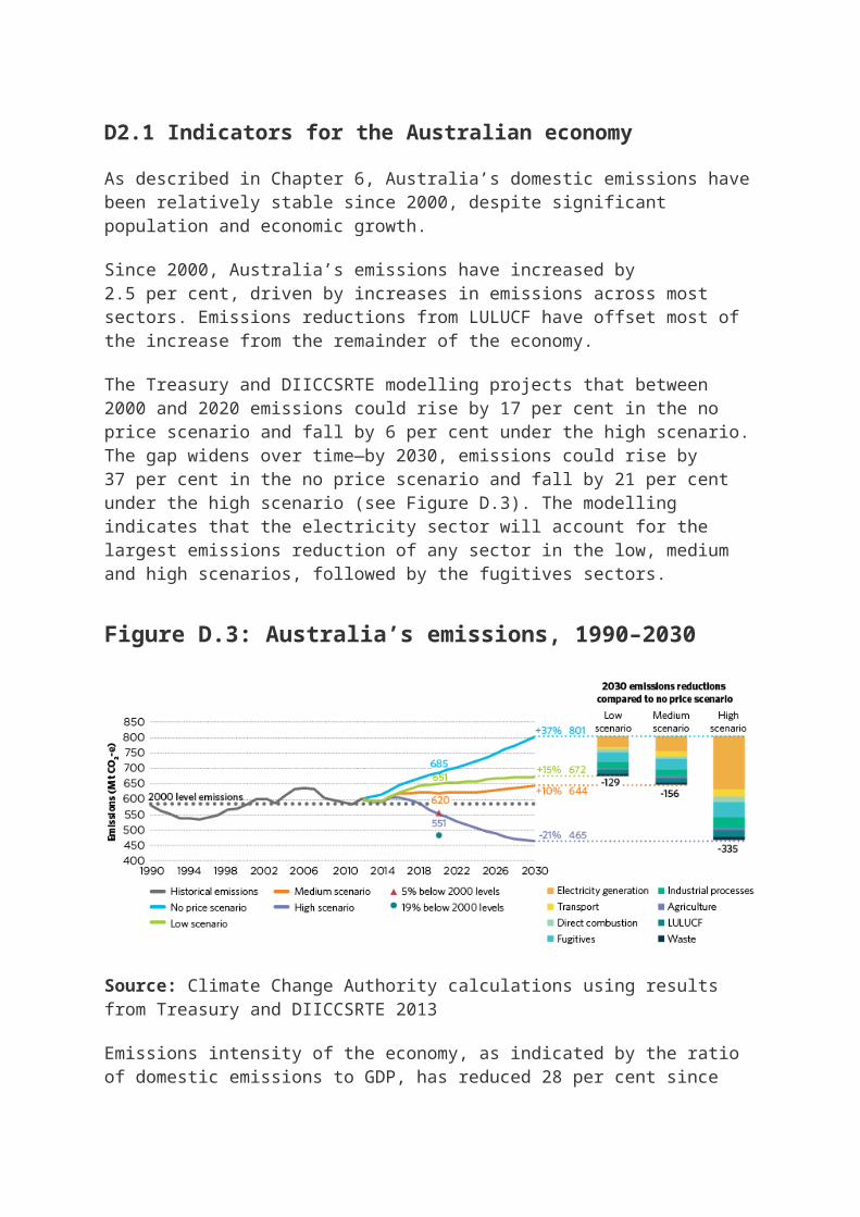
Figure D.5: Australia’s emissions intensity—emissions per unit

GDP ($2012), 2000–2030

 

Source: Climate Change Authority calculations using results from Treasury and DIICCSRTE 2013

Figure D.6: Australia’s emissions intensity—emissions and

population, 2000–2030

 

Source: Climate Change Authority calculations using results from Treasury and DIICCSRTE 2013

D2.2 Overview of sectoral progress

Electricity generation and direct combustion emissions are projected to continue to account for about half of Australia’s total emissions over the

period to 2030. Transport, fugitive and agricultural emissions are forecast to make up the majority of the remaining emissions.

The projected growth in direct combustion, fugitive and agricultural emissions is projected to offset reductions in waste, industrial process and electricity emissions over the period to 2030 in all except the high scenario.

Figure D.7 shows that an emissions reduction of about 134 Mt CO2-e could be achieved in 2020 under the high scenario compared to the no price scenario, which is broadly consistent with the minimum reduction required to deliver the unconditional 5 per cent target.

Figure D.7: Changes in Australia’s emissions—no price and high

scenarios, 2012–2030

 

Source: Climate Change Authority calculations using results from Treasury and DIICCSRTE 2013

D2.3 Sectoral contributions to emissions

State and Commonwealth regulation has been a major driver of emissions reductions. An 85 per cent reduction in LULUCF emissions, largely due to economic conditions and regulatory restrictions on land clearing, was a key reason why Australia’s whole-of-economy emissions were relatively flat between 1990 and 2012. The Treasury and DIICCSRTE modelling does not project similar improvements for this sector in future.

Electricity is the most significant sectoral contributor to emissions. Emissions from electricity generation grew quickly until 2009, when they started to decline. Since then, reduced demand for grid-connected electricity, combined with lower emissions generation, has driven down emissions.

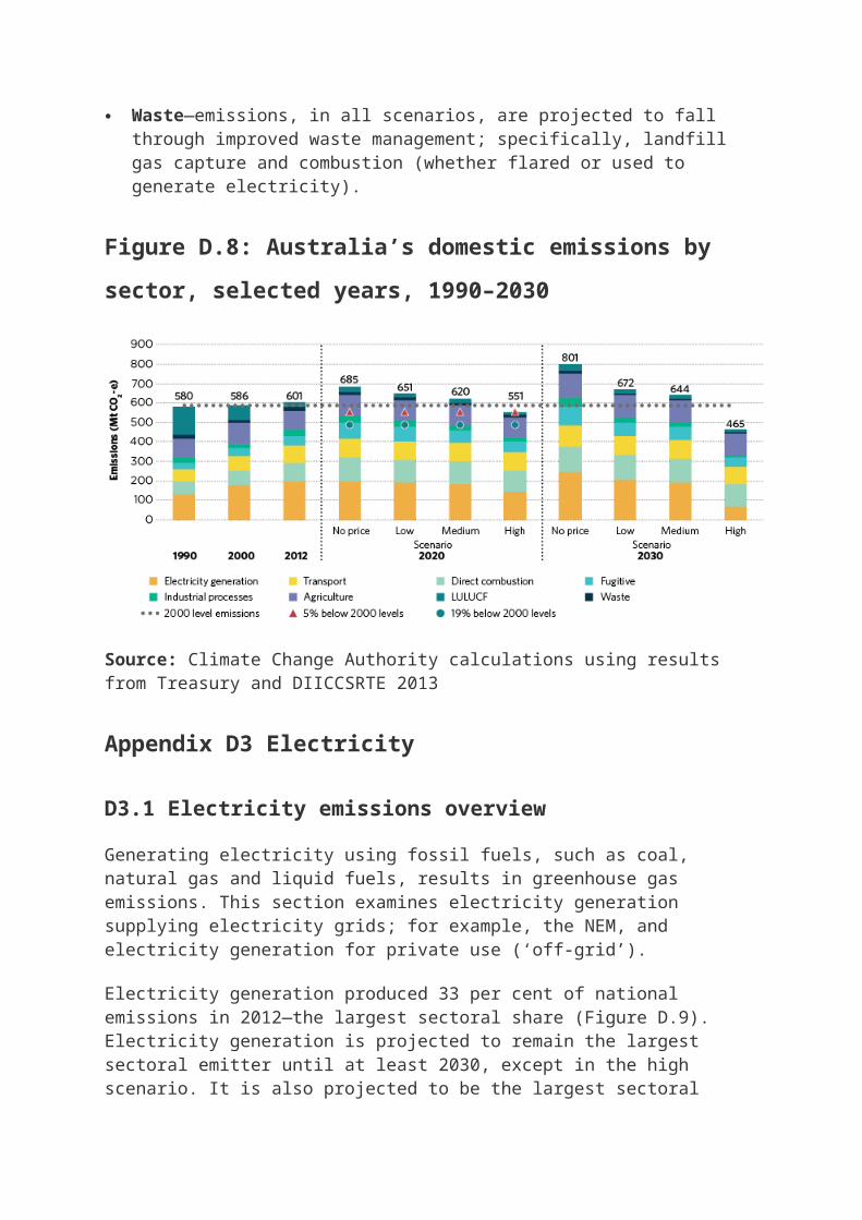
Under the low, medium and high scenarios, reductions in Australia’s emissions intensity between 2012 and 2030 are more distributed across the economy than in the past. These sectoral changes are shown in Figure D.8.

Electricity—emissions under the high scenario are projected to decline to 2030, driven by lower demand growth, energy efficiency and a shift towards lower emissions intensity generation. The outlook under the low scenario and no price scenario is for emissions to rise by between 5 and 23 per cent between 2012 and 2030.

Transport—demand is expected to continue to grow, driven by strong growth in road freight and domestic aviation. Modest growth is projected in light passenger vehicle emissions, which are the largest contributor to transport emissions. Increasing use of low-emissions fuels and vehicle efficiency improvements are projected to partially offset activity increases to 2030.

Direct combustion and fugitive emissions—projected to increase to 2030, particularly because of greater gas production driven by foreign demand for Australian LNG and coal. Growth in these sectors could drive most of the net growth in domestic emissions to 2030 under the low scenario; more than offset the net reductions from the rest of the economy under the medium scenario; or significantly offset the net emissions reduction under the high scenario.

Industrial processes—under the low, medium and high scenarios, industrial process emissions are projected to fall by between 25 and 66 per cent from 2012 to 2030, largely due to the deployment of nitrous oxide conversion catalysts, which improve emissions intensity. Under the no price scenario, industrial process emissions are projected to rise by about 40 per cent above 2012 levels by 2030.

Agriculture and LULUCF—increasing export demand for Australian agricultural commodities is projected to drive an increase in emissions from agriculture. Projected emissions from LULUCF depend on the level of incentive for emissions reductions.

Waste—emissions, in all scenarios, are projected to fall through improved waste management; specifically, landfill gas capture and combustion (whether flared or used to generate electricity).

Figure D.8: Australia’s domestic emissions by sector, selected years,

1990–2030

 

Source: Climate Change Authority calculations using results from Treasury and DIICCSRTE 2013

Appendix D3 Electricity

D3.1 Electricity emissions overview

Generating electricity using fossil fuels, such as coal, natural gas and liquid fuels, results in greenhouse gas emissions. This section examines electricity generation supplying electricity grids; for example, the NEM, and electricity generation for private use (‘off-grid’).

Electricity generation produced 33 per cent of national emissions in 2012—the largest sectoral share (Figure D.9). Electricity generation is projected to remain the largest sectoral emitter until at least 2030, except in the high scenario. It is also projected to be the largest sectoral

contributor to emissions reductions in the low, medium and high scenarios.

Figure D.9: Electricity generation sector share of Australia’s

emissions, selected years, 1990–2030

 

Source: Climate Change Authority calculations using results from Treasury and DIICCSRTE 2013

After decades of growth, levels of electricity generation have been relatively stable since 2008. Since then, emissions have declined by an average of almost 1 per cent each year to 2012. The Australian Energy Market Operator (AEMO 2013a) and Treasury and DIICCSRTE (2013) project that electricity demand will start growing again to 2020 and continue to rise after that (Figure D.10).

Along with lower demand, the recent emissions decline was also due to a marked downturn in emissions intensity of electricity supply (BREE 2013b; Treasury and DIICCSRTE 2013). ACIL Allen Consulting (2013) projects that this trend may continue in the low, medium and high scenarios, but could stall from 2020 in the no price scenario (Figure D.11).

Figure D.10: Electricity generation activity and emissions intensity

of electricity supply—modelled range, 1990–2050

 

Note: Upper and lower line bounds illustrate range of modelled outcomes. Electricity generation activity is ‘as generated’.Source: Climate Change Authority calculations using BREE 2013b and results from Treasury and DIICCSRTE 2013

Figure D.11: Electricity generation activity and emissions intensity

—four scenarios, 1990–2050

 

Note: Electricity generation activity is ‘as generated’. Sources: ACIL Allen Consulting 2013; BREE 2013b; Climate Change Authority calculations using results from Treasury and DIICCSRTE 2013

This section describes the most substantive contributors to and drivers of the emissions outcomes projected for the electricity sector. Results of the four scenarios are presented, as modelled by the Treasury and DIICCSRTE 2013. Appendix D3 focuses on grid-connected electricity,

which accounted for about 96 per cent of total electricity generation in 2011–12; off-grid electricity generation is analysed specifically where relevant (ACIL Allen Consulting 2013).

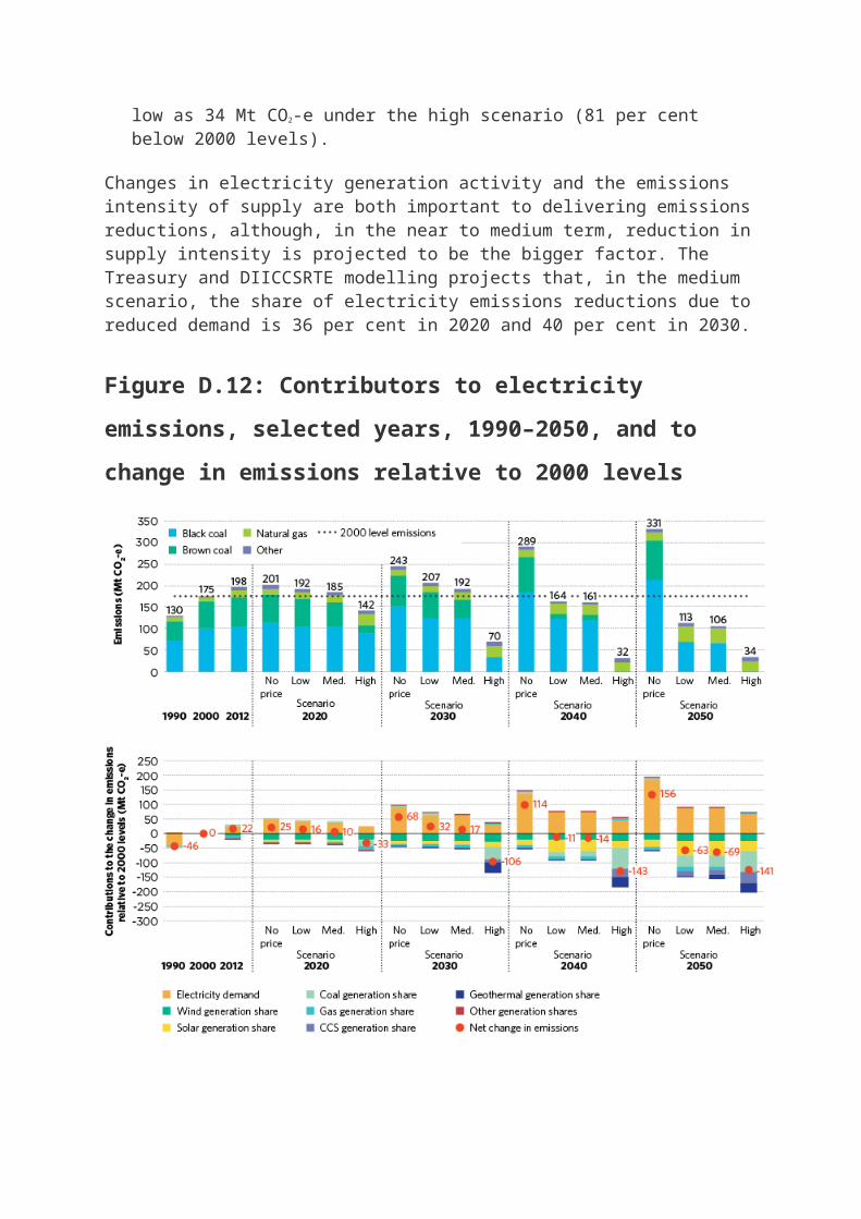
Figure D.12 shows significant growth in electricity sector emissions in the no price scenario, rising to 14 per cent above 2000 levels in 2020, and almost 40 per cent above 2000 levels in 2030.

Targeted policy could substantially reduce the sector’s emissions. The Treasury and DIICCSRTE modelling suggests that higher electricity demand could be offset by a lower emissions intensity of supply in the low, medium and high scenarios, thus reducing electricity sector emissions (figures D.10 and D.11). If a price incentive is in place, the modelling projects that:

In 2020, Australia’s electricity sector emissions are reduced from their 2012 levels (198 Mt CO2-e) to between 142 and 192 Mt CO2-e (high and low scenarios, respectively). For the low and medium scenarios, this is a moderate increase on 2000 emissions levels, but for the high scenario it is a 19 per cent reduction.

In 2030, electricity sector emissions trends are heavily dependent on policy drivers. Emissions could rise to between 192 and 207 Mt CO2-e in 2030 (medium and low scenarios, respectively) or fall under the high scenario to 70 Mt CO2-e in 2030 (60 per cent below 2000 levels).

In 2050, the low and medium scenarios see emissions fall to about 110 Mt CO2-e (37 per cent below 2000 levels) and to as low as 34 Mt CO2-e under the high scenario (81 per cent below 2000 levels).

Changes in electricity generation activity and the emissions intensity of supply are both important to delivering emissions reductions, although, in the near to medium term, reduction in supply intensity is projected to be the bigger factor. The Treasury and DIICCSRTE modelling projects that, in the medium scenario, the share of electricity emissions reductions due to reduced demand is 36 per cent in 2020 and 40 per cent in 2030.

Figure D.12: Contributors to electricity emissions, selected years,

1990–2050, and to change in emissions relative to 2000 levels

 

Source: Climate Change Authority calculations using results from Treasury and DIICCSRTE 2013

D3.1.1 Overview of changes in electricity generation emissions intensity

Emissions intensity of electricity generation declined by about 7 per cent between 2000 and 2012 with further improvement expected in all modelled scenarios. The Treasury and DIICCSRTE projects that, in a no price scenario, the improvement is relatively modest; emissions intensity is about 16 per cent lower than 2000 levels in 2020—primarily as a result of renewables and driven by the RET—but is likely to change little after that.

With incentives in place to reduce emissions, changes in the electricity supply mix could reduce the emissions intensity of supply by up to a third in 2020 and by almost 90 per cent by 2050, compared to 2000 levels (Table D.1).

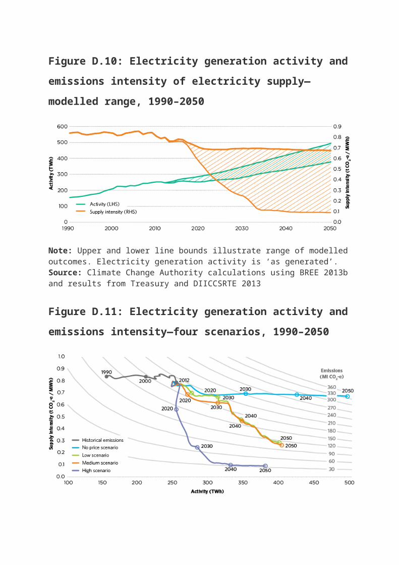
Table D.1: Emissions intensity of Australia’s electricity supply,

2000–2050

  Historical emissions intensity(t CO2-e/MWh)

Projected emissions intensity(t CO2-e/MWh)

Scenario

2000 2008 2012 2020 2030 2040 2050

No price

0.84 0.84 0.78 0.70 0.69 0.69 0.67

Low       0.70 0.66 0.48 0.28

Medium

      0.69 0.62 0.47 0.26

High       0.56 0.25 0.10 0.09

Note: Calculation based on electricity generation ‘as generated’. Source: Historical: BREE 2013b, Table O; DCCEE 2012 Projections: Climate Change Authority based on Treasury and DIICCSRTE 2013 data and ACIL Allen Consulting 2013

Figure D.12 shows several contributors to a lower emissions intensity electricity supply, particularly:

Declining conventional coal-fired generation, which could reduce emissions by between 2 and 56 Mt CO2-e in 2020, relative to 2000 levels. Emissions from coal-fired generation are projected to be higher in 2030 than in 2000, except under the high scenario where they could be almost 130 Mt CO2-e lower.

Increasing wind and solar generation share, which could contribute to an emissions reduction of about 30 Mt CO2-e in 2020, relative to 2000. Projections suggest that in 2030 increasing wind and solar generation could reduce emissions by between 39 and 51 Mt CO2-e (in no price and high scenarios, respectively), relative to 2000.

CCS and geothermal generation could also contribute significantly in later decades, with an incentive in place, though timing of their deployment remains uncertain. Table D.3 provides further detail of the

potential fuel mixes that could lower the emissions intensity of electricity.

The deployment and diffusion of electricity generation technologies will depend on a range of drivers. Exchange rates, technological advances, climate change mitigation policy and electricity prices will affect the relative cost of technologies and the point at which each option becomes economically viable. Until 2020, the mandatory RET is likely to drive steady deployment of renewables, such as wind. Sections D3.3 and D3.4 discuss the opportunities and barriers to realising the potential changes in emissions intensity.

D3.1.2 Overview of changes in electricity demand

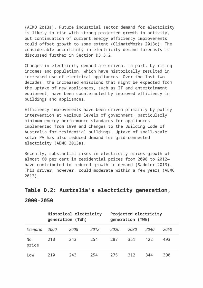
Since 2008, growth in electricity generation has slowed (Table D.2). Macroeconomic drivers, weaker global financial conditions and a rising Australian dollar have underpinned softening demand in the industrial sector, with the closure of the Kurri Kurri aluminium smelter in 2012 being one example (AEMO 2013a). Future industrial sector demand for electricity is likely to rise with strong projected growth in activity, but continuation of current energy efficiency improvements could offset growth to some extent (ClimateWorks 2013c). The considerable uncertainty in electricity demand forecasts is discussed further in Section D3.5.2.

Changes in electricity demand are driven, in part, by rising incomes and population, which have historically resulted in increased use of electrical appliances. Over the last two decades, the increased emissions that might be expected from the uptake of new appliances, such as IT and entertainment equipment, have been counteracted by improved efficiency in buildings and appliances.

Efficiency improvements have been driven primarily by policy intervention at various levels of government, particularly minimum energy performance standards for appliances implemented from 1999 and changes to the Building Code of Australia for residential buildings. Uptake of small-scale solar PV has also reduced demand for grid-connected electricity (AEMO 2013a).

Recently, substantial rises in electricity prices—growth of almost 60 per cent in residential prices from 2008 to 2012—have contributed to reduced growth in demand (Saddler 2013). This driver, however, could moderate within a few years (AEMC 2013).

Table D.2: Australia’s electricity generation, 2000–2050

  Historical electricity generation (TWh)

Projected electricity generation (TWh)

Scenario

2000 2008 2012 2020 2030 2040 2050

No price

210  243 254  287 351 422 493

Low 210  243 254  275 312 344 398

Medium

210  243 254  269 312 346 401

High 210  243 254  253 282 329 378

Note: Electricity generation is ‘as generated’. Source: Historical: BREE 2013b, Table O Projections based on ACIL Allen Consulting 2013

The Treasury and DIICCSRTE’s modelling projects that Australia’s electricity generation will remain steady or rise to 2020 and rise more quickly to 2030, in all scenarios. The effect of the price incentive on projected generation is evident. Electricity generation is about 6 per cent lower in 2020 under the high scenario than the medium scenario. By 2050, electricity generation could be between 80 and 89 per cent higher than in 2000, depending on the level of the price incentive (high and low scenarios, respectively).

Some of the major contributors expected to reduce future emissions, through changing demand in the residential and commercial sectors, have long lead times due to the slow replacement rate of buildings and appliances. These include:

improvements in building efficiency, which could reduce emissions, relative to 2000 levels, by about 12 Mt CO2-e in 2020 and more in later years as stock turns over

improvements in the efficiency of electrical appliances, which could reduce emissions, relative to 2000 levels, by about 20 Mt CO2-e in 2020 and more in later years (DCCEE 2010b, p. 23).

Section D3.3 discusses further the opportunities and barriers to the uptake of cost-effective emissions reductions through changing electricity demand and reducing the level of total generation.

D3.2 Emissions intensity of electricity supply

D3.2.1 Emissions intensity outcomes in an international context

Australia’s emissions intensity of electricity is among the highest in the developed world. It is about four times the intensity of New Zealand and Canada; almost double the intensity of Germany, the UK and Japan; and considerably higher than that of the US. Since 2007, Australia’s electricity supply emissions intensity has exceeded China’s (IEA 2013b).

Table D.1 summarises projections for Australia’s emissions intensity, which, in all scenarios, reflect some improvement on current and historical levels. Despite these projected improvements, in all except the high scenario Australia’s emissions intensity is likely to remain above that of China, the US and the world average in 2035 (IEA 2012a; Treasury and DIICCSRTE 2013).

D3.2.2 Contributors to emissions intensity of generation

With incentives in place, a range of projections suggest that Australia’s electricity supply will become less emissions-intensive as conventional fossil fuel-fired generation loses share to low- and zero-emissions sources. Several technologies could contribute directly to a lower emissions intensity of supply. Changes in the shares of conventional coal-fired generation and renewables could be particularly significant (Figure D.12).

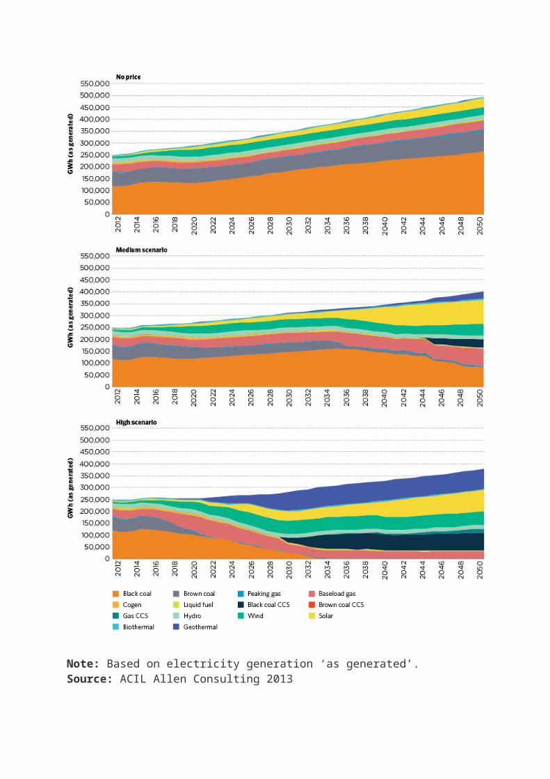
This is illustrated in ACIL Allen Consulting’s outlook for Australia’s electricity supply in Figure D.14. The projected generation mix is affected significantly by the level of the price incentive. The high scenario projects a substantial increase in the share of generation from renewables and a fall in the share of coal-fired generation. Coal with CCS is also deployed by 2030, bringing the emissions intensity of generation down by over 60 per cent compared to the no price scenario, to 0.25 t CO2-e/MWh. By contrast, the low scenario projects relatively modest changes to the supply mix, with emissions intensity of generation projected to be 0.66 t CO2-e/MWh in 2030. The growth in renewable generation, driven primarily by the RET to 2020, is important in all scenarios, even in the no price scenario, where the generation mix is otherwise projected to be little changed.

Figure D.13: Share of electricity generation by fuel type, 2012–2050 

 

Note: Based on electricity generation ‘as generated’. Source: ACIL Allen Consulting 2013

Uncertainties about the timing and magnitude of declines in emissions-intensive electricity generation and growth in low-emissions generation give rise to a range of potential electricity supply mixes for Australia. Table D.3 presents the projected range of generation shares between the no price and high scenarios.

Table D.3: Share of electricity generation for selected fuels and

technologies, 2000–2030 (no price to high scenario)

  Historical Projected

Fuel type 2000 2012 2020 2030

Coal (conventional)

83% 71% 48–67% 9–70%

Natural gas (conventional)

8% 15% 9–25% 8–14%

Coal and gas with CCS

Not available

Not available

Not available

Up to 7%

Potentially deployed as early as 2030 but as late as mid 2040s

All renewable 9% 11% 21–24% 21–69%

Solar Negligible

1% 3% 6–14%

Wind Negligible

3% 11–12% 9–20%

Geothermal Not available

Not available

Not available

Up to 28%

Note: Results are based on shares of generation ‘as generated’ for four modelled scenarios with various levels of price incentive, as described in Chapter 9. All scenarios include the RET as legislated. ‘All renewables’ includes hydro, wind, geothermal, biomass, solar PV and solar thermal. Solar water heating is not included.Source: ACIL Allen Consulting 2013

Off-grid electricity generation, which is generally in regional and remote areas, has a different supply mix. Its emissions intensity is currently lower than for Australia’s as a whole. In 2012, almost 80 per cent of off-grid generation was produced using gas, reflecting the high proportion of energy and resource operations located in areas supplied by gas pipelines (BREE 2013c). Indications are that gas generation will continue to dominate off-grid electricity generation (ACIL Allen Consulting 2013).

Compared with the national average of almost 10 per cent, the share of renewables in off-grid generation was as little as 2 per cent, with the greatest share in the southern states. In Tasmania, New South Wales, Victoria and the Australian Capital Territory, renewables account for 27 per cent of off-grid generation (BREE 2013c, p. 19).

D3.2.3 Drivers of emissions intensity of generation

Several drivers will influence the deployment and diffusion of technologies that determine the emissions intensity of electricity supply. The primary determinant of the supply mix—and how quickly emissions-intensive generators decline and low-emissions generators grow—will be the relative cost of generation from different sources. Coal currently dominates Australia’s electricity supply because it has the lowest marginal costs of operation.

Multiple drivers change the business cases of electricity generation projects. Modelling suggests that policy is a critical influence. The presence of a price incentive for emissions reduction, and the level of that incentive, can make different sources more or less competitive. This is evident from the greater share of low-emissions generation in scenarios with a higher price incentive. The effect of the RET, which provides an additional revenue stream to support the deployment of renewable sources, is also apparent to the 2020s. If the RET was reduced or not met, the emissions intensity of generation would be higher than that projected here.

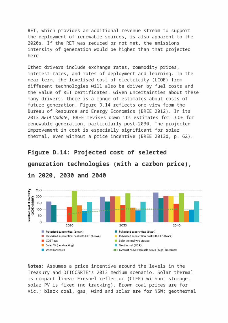
Other drivers include exchange rates, commodity prices, interest rates, and rates of deployment and learning. In the near term, the levelised cost of electricity (LCOE) from different technologies will also be driven by fuel costs and the value of RET certificates. Given uncertainties about these many drivers, there is a range of estimates about costs of future generation. Figure D.14 reflects one view from the Bureau of Resource and Energy Economics (BREE 2012). In its 2013 AETA Update, BREE revises down its estimates for LCOE for renewable generation, particularly post-2030. The projected improvement in cost is especially significant for solar thermal, even without a price incentive (BREE 2013d, p. 62).

Figure D.14: Projected cost of selected generation technologies (with

a carbon price), in 2020, 2030 and 2040

 

Notes: Assumes a price incentive around the levels in the Treasury and DIICCSRTE’s 2013 medium scenario. Solar thermal is compact linear Fresnel reflector (CLFR) without storage; solar PV is fixed (no tracking). Brown coal prices are for Vic.; black coal, gas, wind and solar are for NSW; geothermal is in SA. Source: ACIL Allen Consulting 2013 medium scenario (‘central scenario’) (for NEM prices); BREE 2012 (for LCOE)

To at least 2020, relatively stable demand for grid-connected electricity makes it unlikely that there will be significant investment in electricity generation, except in response to policy drivers such as the RET (AEMO 2013g). During this period, existing generators, which have already amortised their initial capital investment, will be likely to continue to operate. This means that the risk of ‘lock-in’ of new high-emissions generation is relatively low for the next 10 years.

Longer term, as economic activity grows and electricity demand rises, new generation will be needed. Capital and regulatory hurdles aside, lower cost generation sources will be taken up more quickly and deployed more widely. Given the long operating life of electricity generators, future fleet investment choices are likely to influence Australia’s emissions for decades. Investment plans of major energy sector players, however, suggest building new emissions-intensive coal-fired plants is unlikely (see, for example, AGL 2013, pp. 37–8).

When the drivers that affect technology costs change, so do the projected electricity generation mix and projected emissions, as shown in

Table D.4. Findings of ACIL Allen Consulting’s (2013) modelling sensitivities include:

A higher price incentive will see greater emissions reductions. The share of coal will fall more quickly and coal-fired plants retire sooner, and the share of low-emissions electricity generation, including renewables and CCS, could be larger.

A higher price for gas, oil and coal will have an uncertain effect on emissions, depending on the relative prices for these fuels at different times. Since fuel prices usually comprise a greater share of generation costs for gas-fired generators than coal-fired generators, higher fuel prices may disadvantage gas over coal. Higher fuel prices would also disadvantage fossil-fuelled generators over renewables by the late 2020s, leading to a fall in emissions.

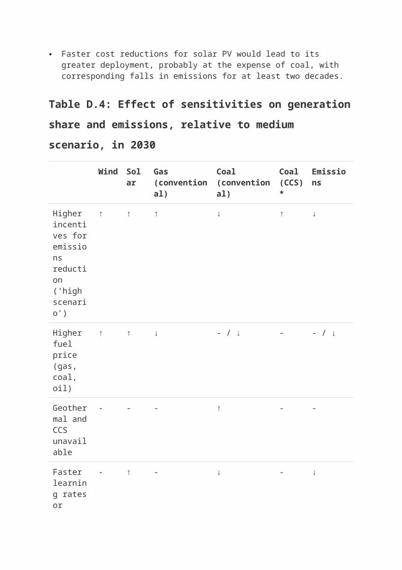
Faster cost reductions for solar PV would lead to its greater deployment, probably at the expense of coal, with corresponding falls in emissions for at least two decades.

Table D.4: Effect of sensitivities on generation share and emissions,

relative to medium scenario, in 2030

  Wind

Solar

Gas (conventional)

Coal (conventional)

Coal (CCS)*

Emissions

Higher incentives for emissions reduction (‘high scenario’)

↑ ↑ ↑ ↓ ↑ ↓

Higher fuel price (gas, coal, oil)

↑ ↑ ↓ - / ↓ - - / ↓

Geother - - - ↑ - -

  Wind

Solar

Gas (conventional)

Coal (conventional)

Coal (CCS)*

Emissions

mal and CCS unavailable

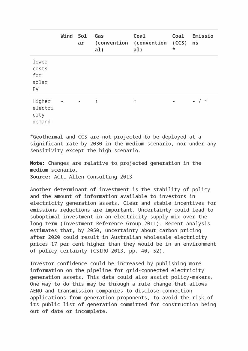
Faster learning rates or lower costs for solar PV

- ↑ - ↓ - ↓

Higher electricity demand

- - ↑ ↑ - - / ↑

*Geothermal and CCS are not projected to be deployed at a significant rate by 2030 in the medium scenario, nor under any sensitivity except the high scenario.

Note: Changes are relative to projected generation in the medium scenario. Source: ACIL Allen Consulting 2013

Another determinant of investment is the stability of policy and the amount of information available to investors in electricity generation assets. Clear and stable incentives for emissions reductions are important. Uncertainty could lead to suboptimal investment in an electricity supply mix over the long term (Investment Reference Group 2011). Recent analysis estimates that, by 2050, uncertainty about carbon pricing after 2020 could result in Australian wholesale electricity prices 17 per cent higher than they would be in an environment of policy certainty (CSIRO 2013, pp. 40, 52).

Investor confidence could be increased by publishing more information on the pipeline for grid-connected electricity generation assets. This data could also assist policy-makers. One way to do this may be through a rule change that allows AEMO and transmission companies to disclose connection applications from generation proponents, to avoid the risk of its public list of generation committed for construction being out of date or incomplete.

D3.3 Emissions reduction opportunities from existing generation

D3.3.1 Fossil-fuelled generation

To at least 2020, existing and committed electricity supply is expected to be adequate to meet demand in the NEM (AEMO 2013b). This, combined with uncertainty in policy and fuel prices, is likely to lead to only incremental or small-scale change in the electricity sector.

In the near term, the main opportunities to reduce the emissions intensity of the existing generation fleet may relate to:

reducing output

retrofitting

fuel prices.

Reducing output

The recent trend in coal-fired generation has been for plants to reduce output rather than retire. Since 2009, over 2,000 MW of coal-fired generation has been mothballed and coal-fired asset utilisation was down, with black coal falling from 86 to 79 per cent between 2007 and 2013 (ClimateWorks 2013b, p. 25). Some black coal-fired plants are operating as low as 30–45 per cent of capacity (Pitt & Sherry 2013). If stable demand and policy uncertainty delay investment in large new sources of supply, this pattern may continue until the early 2020s. AEMO estimates that between 3,100 and 3,700 MW—or up to 12 per cent—of coal-fired capacity connected to the NEM may be removed by 2020 in scenarios without or with a carbon price (2013g, p. iv).

It is possible that some generators would change business models to run plants as intermediary generation, or operate during summer when wholesale prices are generally higher, rather than close completely (CCA 2013). A wide range of modelling studies suggest this is possible, with conventional coal projected to remain in Australia’s electricity supply mix for decades, even if a price incentive to reduce emissions exists.

Exit costs could present a barrier to retiring existing fossil fuel plant. Clean-up and remediation requirements, which take effect upon closure, could cost hundreds of millions of dollars, improving the case for operating for longer, even at reduced output (AECOM 2012; Colomer 2012).

There is a consistent outlook, across a range of modelling studies, that when a price incentive for emissions reduction exists, coal-fired generation falls. ACIL Allen Consulting (2013) suggests that the share of generation from conventional coal could fall from 71 per cent now to as low as 48 per cent in 2020 and 9 per cent in 2030 (Table D.3). Timing is uncertain, but ACIL Allen Consulting (2013) projects the fall will occur in the late 2030s for black coal and as soon as the early 2020s for brown coal, in the low and medium scenarios. Under a high scenario, coal-fired generation would fall earlier and more sharply. In contrast, without a price incentive, ACIL Allen Consulting (2013) projects coal could continue to be about 70 per cent of generation in 2030. Some analysts suggest that, without price incentives, existing coal-fired generators (particularly brown coal) could gain market share, partly at the expense of gas-fired generators, which face rising fuel costs (RepuTex 2013).

Retrofitting

Some fossil fuel generators may also be retrofitted to operate with lower emissions intensity. Several Australian coal-fired generators have indicated plans to upgrade turbines, modify boiler operation and investigate coal-drying technologies to improve thermal efficiency and reduce emissions (DRET 2013).

Retrofitting low-efficiency coal-fired units to operate with high-efficiency, low-emissions coal technologies is another option. This is likely to be relatively costly, but the IEA suggests it could be considered on a case-by-case basis and could potentially reduce the emissions intensity of coal-fired generation to 0.67–0.88 t CO2/MWh (IEA 2012d, p. 15).

There also appears to be significant potential to retrofit existing fossil fuel plants with hybrid technologies. Co-firing with lower emissions fuels not only cuts emissions but also overcomes traditional barriers to renewable energy, including land availability, capital and transmission costs. An early step has already been taken by the 2,000 MW black coal Liddell Power Station, which has installed an 18 MW solar thermal array to heat water to create steam, thus reducing the need to burn coal for that purpose, cutting emissions by approximately 5,000 tonnes each year (EcoGeneration 2013). In addition, Liddell can co-fire coal with biomass and recycled oil (Macquarie Generation 2012). In their Clean Energy Investment Plans submitted to the Commonwealth Government, other generators, including Loy Yang, indicate that they are investigating the potential for co-firing (DRET 2013).

Fuel prices

For existing fossil fuel generation technologies, fuel prices are a major determinant of cost and will affect how coal- and gas-fired generation contribute to Australia’s supply mix. As Australia’s gas production booms and eastern Australia prepares to export LNG for the first time, gas price rises are anticipated, though the timing and precise levels are uncertain (Wood and Carter 2013). In some scenarios, even with a price incentive in place, the Treasury and DIICCSRTE modelling suggests that projected increases in gas prices could make existing gas power plants more costly than coal-fired power. Modelling of a high gas price suggests the share of base-load gas generation could fall below its current share and below its projected share in 2020 or 2030 in the medium scenario. This trend could also occur if coal prices fell, as observed in the UK during 2012 (Kerai 2013).

Overseas, lower cost gas is increasing its share in electricity generation by displacing coal, and reducing emissions as a result. In the US, increasing generation from natural gas contributed to a decline in emissions from electricity generation of 4.6 per cent in 2011 compared to the previous year (US EPA 2013). Australia’s gas prices are considerably higher—and likely to rise more in coming years—making this change in supply mix less likely. AEMO, for example, does not foresee an increase on current levels of gas use in Australia’s eastern states until about 2030 (AEMO 2013f).

Major electricity sector players report that it may not be economical to build a large new grid-connected gas-fired power plant for the foreseeable future (CCA 2013). This is reflected in AEMO’s Gas Statement of Opportunities, which suggests the use of gas in electricity generation will fall significantly over the next few years, as gas prices rise (AEMO 2013f).

The economic viability of new coal-fired generation facilities may be undermined by difficulty in obtaining low-cost finance, if the international trend of withdrawing finance to coal-fired generators extends to Australia. In mid 2013, the US Export-Import Bank, the World Bank and European Investment Bank, which together provided more than $10 billion for coal projects in the last five years, announced they would withdraw from financing conventional coal (Drajem 2013).

D3.3.2 Generation from renewable energy

ACIL Allen Consulting (2013) projects significant amounts of renewable generation under a range of scenarios (see Table D.3). The RET drives the deployment of renewable energy to 2020 in all scenarios, including the no price scenario. The addition of a carbon price in the low, medium and high scenarios results in significantly more renewable generation.

Figure D.13 shows that after 2020 the increase in renewables is projected to be much greater with a higher price incentive.

Wind is likely to increase its share of the supply mix in the near term. To 2020, wind is expected to provide about 84 per cent of new generation capacity, largely reflecting the impact of the RET (AEMO 2013g). In late 2012, 65 per cent of the 3,000 MW of planned installed electricity capacity at an advanced stage of development was wind (BREE 2013a).

Australia’s solar resource is one of the best in the world and theoretically capable of generating enough electricity to meet its demand (Geoscience Australia and ABARES 2010). Solar PV systems might offer consumers financial savings by reducing consumption of grid-connected electricity. The value of solar PV is likely to be greatest for users with an electricity demand profile that matches system output, such as commercial premises (Wood et al. 2012). Solar PV’s low reliance on water makes it viable even in dry and remote locations, and in a future with potential disruption to water supply (see Box D.2).

Box D.2: Climate change effects on electricity supply

Climate change will affect future opportunities to change the electricity supply mix and reduce emissions. Its impacts, particularly water shortages and extreme weather, affect electricity demand, generation and transportation (Foster et al. 2013; Senate Environment and Communications References Committee 2013). Sources of generation that use large amounts of water, including coal-fired and nuclear power, geothermal and bioenergy, will be disadvantaged in a context of water shortages (IEA 2013c).

Over the last decade, Australian electricity supply has been disrupted by floods and bushfires. The output of hydroelectric and coal-fired generators, which use large amounts of water for steam production and cooling, have been reduced and could fall again with drought. With water shortages and more extreme climate events expected (see Chapter 2), the extraction of coal and unconventional gas, generation from certain sources, and the transmission and distribution of electricity could be disrupted more often (IEA 2013c; US DoE 2013).

Solar generation is projected to play a large role in Australia’s future generation mix, particularly in scenarios with a price incentive to reduce emissions. The medium scenario suggests that solar generation could increase its share from about 3 per cent in 2020 to about 20 per cent in 2040 and 25 per cent in 2050. Most of the expected growth is large-scale generation.

If costs continue to fall, solar PV could become increasingly cost-competitive with conventional sources of generation. ACIL Allen Consulting (2013) modelled a sensitivity that reduced the costs, per annum, of large-scale solar PV by 10 per cent to 2020 and 5 per cent to 2030. The results showed that solar PV could generate almost six times as much electricity in 2020 and 35 times as much in 2030, when compared to 2012.

D3.4 Reducing emissions with emerging generation and storage options

Current excess generation capacity, combined with uncertainty about emissions reduction policy and fuel costs, makes it unlikely that new electricity generation technologies will emerge in Australia, at scale, before at least 2020.

Large uncertainties remain about the timing, costs and viability of new low-emissions sources of electricity generation, particularly CCS and geothermal. Previous modelling suggested a greater role for these technologies (for example, SKM-MMA 2011 and ROAM 2011). In contrast, ACIL Allen Consulting (2013) suggests that in the low or medium scenarios, neither CCS nor geothermal will contribute a significant share of generation until about 2040. The high scenario suggests, however, that geothermal and CCS may emerge as early as 2017 and 2030, respectively.

The technology and business models necessary to widely deploy electric storage are changing rapidly, making cost and uptake highly uncertain.

D3.4.1 Carbon capture and storage for coal- and gas-fired generation

CCS is not yet operating at a large scale1 for electricity generation anywhere in the world, though it has been deployed in the gas processing and industrial sectors (see appendices D6 and D7). The gradual progress in developing large-scale projects is evident in the Global Carbon Capture and Storage Institute’s status reports. Between 2010 and 2013, the number of operational projects did not change and the total CO2 capture capacity of all identified large-scale integrated projects fell (2013c, p. 2). In 2013, the IEA warned that current efforts to develop CCS are ‘insufficient’ and called for ‘urgent action … to accelerate its deployment’ (2013a, pp. 1, 10). The IEA suggests that multiple demonstration projects, each sequestering about 0.8 Mt CO2-e annually, are needed this decade if CCS is to fulfil its emissions reduction potential, consistent with limiting average global temperature increases to 2 degrees (2013a, p. 9).

There are two key challenges to the widespread deployment of CCS for electricity generation. The first is financial—the significant cost to build and operate the technology at a large scale (IEA and GCCSI 2012). The minimum cost for a large-scale CCS plant in Australia will likely be several billion dollars (GCCSI 2013d). The financial barrier may be overcome if an additional revenue stream is available to offset costs of the project, such as enhanced oil recovery (EOR) or a commercial application in other production processes, or if public or policy support is available (GCCSI 2013b).

The second key challenge is the integration of technological components at scale (IEA and GCCSI 2012). The logistical, practical and commercial challenges are likely to be overcome as experience grows, and CCS projects already illustrate this.

There is broad consensus that CCS technology will be first commercially deployed overseas and Australia will be a ‘technology taker’. International developments are likely to set the timing of commercial CCS deployment in Australia. In particular:

China—in many of its significant strategic development and scientific documents, the Chinese Government has expressed strong support for deployment of CCS. China is the only global region where the number of large-scale integrated CCS projects increased between 2011 and 2013, many of them driven by state-owned energy companies (GCCSI 2013a, 2013c).

North America—about 70 per cent of the world’s active large-scale integrated CCS projects are here. Canada’s Boundary Dam and Mississippi Power’s Kemper County projects are expected to operate from early 2014 (GCCSI 2013c; BNEF 2013). Success with these projects would be an important milestone towards the commercialisation of CCS and cost reductions. North America has particular potential because of its high level of committed public support, the commercial opportunities for EOR and an existing CO2 pipeline, which together lower costs and commercial risk (Abellera 2012). New emissions intensity regulations for power plants could provide further incentives.

Australia, with its unique geology, cannot rely on international developments to facilitate storage, however, and will need local expertise.

D3.4.2 Geothermal energy

Australia’s geothermal resource is relatively deep and it is uncertain how and when energy can be extracted reliably, at reasonable cost. Expert estimates of the date of commercial deployment of geothermal energy have been repeatedly revised back. AEMO (2013g) recently suggested commercial geothermal energy developments would not appear in the NEM until after the late 2030s.

The development of Australia’s geothermal energy remains at the exploration and demonstration stage; the most developed project is the 1 MWe Habanero Pilot Plant in South Australia, which produced Australia’s first Enhanced Geothermal Systems (EGS) generated power during a 160-day trial in 2013. Engineering challenges remain for Australia’s geothermal energy, including repeatedly creating heat reservoirs, improving drilling practices and equipment, and enhancing flow rates (Wood et al. 2012).

A major barrier for the development of geothermal generation is the capital outlay needed to trial technology at a large scale. Present estimates suggest a 100 MW hot sedimentary aquifer (HSA) geothermal plant could cost about $700 million (BREE 2012, p. 54). Government funding has played a central role to date. ARENA has committed funding towards demonstration of larger power stations which, if taken up, could provide an opportunity to better understand project costs and the ability to overcome engineering challenges at scale.

D3.4.3 Nuclear fission

Under different circumstances, nuclear fission could play a role in a low-emissions electricity supply mix, as it does overseas. This is apparent in analyses, such as the CSIRO eFutures, in a scenario with a moderate emissions reduction incentive. Even if nuclear power was legalised in Australia, a range of barriers to its deployment remain for large-scale projects (Commonwealth of Australia 2006). These include:

Regulatory and planning requirements—in 2012, Wood et al. concluded that ‘the lead time to deploy a nuclear power plant in Australia is between 15 and 20 years’ because of the need to create legal and regulatory frameworks, and because of time necessary for planning and construction (p. 71). BREE recently estimated that nuclear energy could not be constructed in Australia until 2020 at the earliest (2013d).

Community opinion—it seems that public support would be essential for nuclear power to be viable, though public acceptance remains uncertain and has historically been hostile to the domestic development of nuclear energy (National Academies Forum 2010).

Workforce availability—Australia lacks personnel with the knowledge and capability to plan, construct and operate nuclear power generation. There is also a looming global shortage of these skills (Commonwealth of Australia 2006; OECD 2012).

Nuclear project costs for Australia are uncertain and vary widely, but high costs appear a barrier to deployment in the near term. Recent estimates for developed country nuclear energy projects range from $3–6 million per megawatt (overnight cost, in Wood et al. 2012, p. 711). These costs are high compared to other existing sources of generation. Like geothermal and CCS, nuclear power is capital-intensive and may be difficult for the private sector to finance (Citigroup Global Markets 2009). A report prepared for the Prime Minister in 2006 concluded that to be competitive with existing generation, nuclear power would require a carbon price (Commonwealth of Australia, p. 6). BREE’s 2013 AETA Model Update suggested capital costs of nuclear had risen further since its previous estimates (BREE 2012).

At present, it seems doubtful that planning and capital requirements for nuclear power could be overcome soon enough for it to compete with other low-emissions technologies for which costs are falling, such as solar thermal with storage. If small modular reactors become commercially viable in the short term, however, they could offer a less costly form of nuclear technology than large-scale plant (BREE 2012). Modular reactors also reduce construction timeframes and could allow for more flexible deployment, including in remote locations.

D3.4.4 Electric storage and changes to the electricity grid

Modular storage lends itself well to supporting the generally modest changes expected in Australia’s electricity supply and demand over the next decade. Storage options include batteries (such as those in electric cars) and compressed air. Affordable storage could dramatically improve the economic viability of renewables with variable generation, particularly off-grid (Marchment Hill Consulting 2012). CSIRO analysis suggests that the availability of storage as a backup technology could contribute up to an additional 10 per cent to renewable share and about 20 Mt CO2-e emissions reductions in 2050 (Graham, Brinsmead and Marendy 2013, p. 17).

Storage has been used successfully at scale, such as in Australia’s Smart Grid, Smart City project, but remains relatively costly. A recent EPRI study suggested break-even capital costs of energy storage of between $1,000 and $4,000 per kilowatt (2013, p. v). As with other emerging technologies, overseas developments are relevant to Australia. If California’s target for up to 1.3 GW of storage is realised by 2020, cost

improvements are likely to occur (Reddall and Groom 2013). Government support in Germany and Japan is also accelerating deployment of small-scale and large-scale electric storage, respectively (Parkinson 2013b, 2013c). The CSIRO (2013) estimates that battery costs may halve by 2030, leading to electric storage becoming more widespread. The Authority agrees with the CSIRO’s suggestion that BREE’s Australian Energy Technology Assessment should track developments in small-scale generation and storage technologies.

Australia can learn from successful overseas business models. In New Zealand, for example, electricity distribution network businesses are deploying and operating solar PV and battery storage systems, with leasing arrangements (Parkinson 2013a). Their recent emergence in Australia may increase further uptake of PV, particularly in the commercial sector (Photon Energy 2013). Such business models may help overcome capital hurdles to cost-effective investment. Changes to energy market regulation in Australia could encourage distribution businesses to invest in storage when cost-effective (see Table D.5).

The analysis of electricity sector in this Review is based on modelling and other sources that assume a broad continuation of the existing centralised structure of Australia’s electricity supply. As small-scale and renewable generation increase and costs of electric storage fall, closer examination of a smarter and more decentralised energy system is warranted. The CSIRO’s Future Grid Forum provides one such analysis. Across its four scenarios, it projects:

declines in grid-connected electricity generation from about 2040, with on-site generation to provide between 18 and 45 per cent of generation by 2050

decreasing electricity sector emissions to 55–89 per cent below 2000 levels by 2050 (CSIRO 2013, p. 15).

Box D.3: A zero-emissions supply mix?

Modelling by the Treasury and DIICCSRTE illustrates a potential supply mix where the electricity sector (and other sectors) responds to emissions reduction incentives, at lowest cost and within existing policy parameters. Other studies consider a possible zero-emissions electricity supply mix. For example, AEMO published an exploratory study of a 100 per cent renewables mix, which suggested that there are no technical barriers to such an outcome by 2050. That scenario could be possible without any electrical storage, though it could require ‘generation with a nameplate capacity of over twice the maximum

customer demand’ or a large contribution from biofuel, which faces considerable barriers (AEMO 2013c, p. 4).

With growing deployment of renewables, there is evidence that a generation mix dominated by renewable energy is technically possible. King Island, for example, produces 65 per cent of electricity consumed from renewables, primarily wind. It plans to move towards 100 per cent, combining this generation with solar, biodiesel, battery storage and smart grid technologies (Guevara-Stone 2013). Other studies of high penetration of intermittent renewables, such as solar PV, have found that solutions to grid integration issues, such as new system invertors or electric storage, are available—though at a cost (Brundlinger et al. 2010; Energy Networks Association 2011). Storage that is integrated into large-scale renewables generation, such as solar thermal, is also available.

D3.5 Electricity demand

D3.5.1 Activity emissions outcomes

Activity throughout the economy will affect the levels of electricity demand and the level of emissions. Historically, growth in electricity sector emissions has increased as a result of strong growth in electricity demand (thus increasing total generation levels). From 1990 until a few years ago, Australia’s rate of increase in electricity generation was higher than most developed countries and well above the OECD average (IEA 2013b, p. 107). In 2011, Australia’s annual electricity consumption, per person, was about 11 MWh, above the OECD average of 8 MWh—though lower than the electricity-intensive economies of Canada and the US (IEA 2012b, pp. 70, 74).

The short-term outlook is for Australia’s growth in electricity demand to increase (driven largely by the Queensland resource sector), as illustrated for the NEM in Figure D.15. Many electricity industry stakeholders suggest that, based on their observations of drivers of electricity demand, the low-demand scenario from AEMO is more likely than its medium-demand scenario, and even this may be an overestimate (CCA 2013). AEMO recently revised its short-term forecasts for NEM demand downwards (AEMO 2013e). Electricity demand is projected to remain stable or fall between 2012 and 2020 with a strong emissions reduction incentive in the Treasury and DIICCSRTE’s high scenario.

Even though overall electricity demand is projected to grow, per person electricity consumption is projected to fall to about 9.8 MWh in 2030 in the medium scenario. By contrast to NEM and total Australian electricity demand, it is likely that off-grid electricity generation will grow more

rapidly, as it has in recent years, driven largely by an increasing number of remote resource projects.

Figure D.15 reinforces the fact that changes in electricity generation activity are affected by the level of incentive to reduce emissions. Resulting decreases in demand could provide significant emissions reductions.

Figure D.15: Projected change in NEM demand and per person

electricity consumption, 2013–2030

 

Note: Based on sent out generation for NEM only (which accounts for about 86% of total domestic demand), ACIL Allen Consulting 2013, for 2011–12. Sources: AEMO 2013a; Climate Change Authority calculations using results from Treasury and DIICCSRTE 2013 and the medium scenario from ACIL Allen Consulting 2013

Recently, there has been heightened uncertainty in electricity demand projections, as actual consumption continues to deviate from long-term trends. Several downward revisions to demand projections in recent years illustrate this in the NEM (AEMO 2013a, 2013e). If electricity demand is even lower than projected, it will reduce the size of Australia’s emissions reduction task, all else being equal. Some plausible scenarios for lower electricity demand from households, commercial buildings and industry could keep electricity demand at 2012–13 levels in 2020 and deliver up to 23 Mt CO2-e emissions reductions in 2019–20 (ClimateWorks 2013c, pp. 3, 10).

D3.5.2 Contributors and drivers

Electricity demand is the function of a long list of drivers. Near-term influences on electricity demand are as diverse as the time of year, weather, use of electrical appliances and personal income. Longer term drivers include population growth composition and geographic distribution, electricity prices, economic growth, interest rates and exchange rates, climate change impacts, renewal of building stock, and commercial and industrial activity (Yates and Mendis 2009).

Policies, including energy performance standards, have significantly reduced electricity demand. Some analyses suggest energy efficiency policies have been responsible for more than a third of electricity demand reduction in the NEM between 2006 and 2013 (see, for example, Saddler 2013). Such policies can continue to reduce demand and electricity sector emissions. Because it can be years or decades before equipment and buildings are turned over, future emissions reductions achieved through reduced energy demand will be influenced by the policies and standards put in place in the near term.

Industrial demand

In the medium scenario, the Treasury and DIICCSRTE (2013) projects stable or modestly increasing industrial electricity demand due to:

new activity in major LNG projects in Queensland, coming online from 2014 to 2016

declining activity in energy-intensive manufacturing, particularly aluminium production, as existing contracts for relatively low-priced electricity end

potential reductions in demand through improvements to processes and technologies

additional changes in the composition of the economy, which will see some electricity-intensive industries contract and others expand.

Industrial activity will be driven by several underlying factors, including commodity prices, exchange rates, fuel prices, management processes and the age of infrastructure.

Energy efficiency among large industrial users has increased significantly in recent years and saved users hundreds of millions of dollars. This has been, in part, driven by the Commonwealth Government’s Energy Efficiency Opportunities Program (Department of Industry 2013). It is possible that continued efficiency improvements will reduce industrial electricity use and associated emissions. If the improvements in industrial energy efficiency since 2007–08 are

maintained, ClimateWorks estimates that it could reduce electricity sector emissions by about 6 Mt CO2-e between 2012 and 2020 (2013c, pp. 6, 13).

A sizeable portion of industrial electricity demand is not connected to major electricity grids. BREE reports that the resources and energy sectors, for example, consume off-grid electricity equivalent to about 5 per cent of total national electricity demand (2013c, p. 7). A shift towards off-grid electricity generation has been recently observed and some expect this to continue (ClimateWorks 2013c).

Residential and commercial demand

Since 2008, electricity demand has been flat, despite economic and population growth. Recently, residential, commercial and light-industrial demand for grid-connected electricity has fallen, contributing to emissions reduction. As described in Chapter 6, this has been driven by energy efficiency policy interventions, an increase in household solar PV generation and energy conservation behaviour in response to higher electricity prices (AEMO 2013a; DCCEE 2012; Saddler 2013). While projected growth in population and GNI will put upwards pressure on future electricity consumption, other drivers will dampen demand. Though it is possible the rebound effect could increase demand to some extent, policy and consumer behaviour make it possible that residential and commercial demand, per person, may have peaked for the foreseeable future.

Energy performance standards for buildings and electrical appliances are becoming more stringent and are steadily expanding to cover new products, delivering energy savings, corresponding emissions reductions and cost savings. At the same time, those that been in place for many years are having a noticeable impact over time as the stock of appliances and buildings is turned over and the most inefficient, energy-intensive stock is phased out (Saddler 2013). AEMO reports that, in 2029–30, minimum energy performance standards for electrical appliances could save about 42 TWh and building-related energy efficiency measures could save about 16 TWh electricity (AEMO 2013d, pp. 5–46). The impact could be increased by improving the monitoring and enforcement of building and appliance standards to ensure that they deliver intended energy saving outcomes (DCCEE 2010a).

Driven by standards but also changing preferences, consumers are beginning to move towards less energy-intensive appliances. Large energy savings can come from technology-switching, such as replacing plasma with LCD and LED televisions; incandescent with fluorescent and

LED lighting; conventional electric-resistive water heaters with solar and heat pump systems; and desktop computers with laptops and tablets.

Consumers could further reduce or shift time of demand if governments and regulators make available the information, price incentives and technology discussed in D3.5.3.

Potential new sources of electricity demand

There could be emerging sources of electricity demand from activities that currently use other sources of energy. The uptake of electric vehicles in road transport, already underway, may appreciably increase grid electricity demand from about the mid 2020s. Under the high scenario, where there is a stronger incentive for electric vehicles, electricity consumed for transport in 2050 could be almost double that under all other scenarios (Treasury and DIICCSRTE 2013). Similarly, a shift from gas turbines and motors to electric motors in industry could increase electricity demand. This could see activity and emissions shift from the transport and direct combustion sectors, respectively, to the electricity sector. The relative prices of fuels—petrol, diesel, gas and coal, and electricity—are likely to affect the rate and timing of these shifts. A gas to electricity shift could also be triggered by a possible gas supply shortfall in some locations, as early as 2018–19, and rising gas prices (AEMO 2013f). It is possible that desalination will also present a new source of electricity demand, particularly in a future where water is likely to be scarcer (Foster et al. 2013).

D3.5.3 Further opportunities for cost-effective emissions reduction

Changing energy demand could offer some of the cheapest opportunities for reducing electricity sector emissions (ClimateWorks 2013a; Garnaut 2008; Prime Minister’s Task Group on Energy Efficiency 2010). It can be quick to implement, particularly using existing technologies and practices, and savings can be significant and provide rapid returns on investment (UNEP 2013).

The opportunity to reduce emissions from lowering electricity demand is particularly important in the short term. The IEA’s modelling offers a perspective on the global potential—it projects that energy efficiency measures, through improved lighting and appliances, could provide about 40 per cent of estimated global emissions reductions in 20202 (2013c, p. 54). This is reinforced by UNEP, which points out that improved energy efficiency is one of the characteristics common to scenarios that allow the world to meet a 1.5 or 2 degree target (2013, p. xiii).

The Treasury and DIICCSRTE modelling framework does not reflect all the opportunities to reduce electricity demand. International experience and other analyses show that there are unrealised opportunities to lower electricity sector emissions by reducing electricity demand through energy efficiency. Compared to countries with similar GDP per capita and human development index rankings, Australia lags on energy efficiency and productivity. The IEA reported that, in both 2009 and 2011, Australia has been behind other countries including the US, the UK, Japan and Canada in implementing applicable IEA recommendations (IEA 2012c, p. 478). Though Australia performs comparatively well on lighting, appliance and equipment improvements, the IEA noted that buildings offer a particular opportunity for improvement (2012c, p. 1,223). Box D.4 discusses this potential.

Box D.4: Emissions reduction opportunities in buildings

About 18 per cent of Australia’s emissions are accounted for by buildings’ use of grid-supplied electricity. Slightly more than half are attributable to residential buildings, and the rest to commercial premises (ClimateWorks 2013c, p. 12).

Building-related emissions can be reduced by improving the thermal performance of the building envelope, increasing the efficiency of equipment and appliances, and increasing generation of energy on-site from renewables (such as solar PV) or gas:

Improving building efficiency could reduce emissions, relative to 2000 levels, by 12 Mt CO2-e in 2020.

Improving the efficiency of electrical appliances could reduce emissions, relative to 2000 levels, by 20 Mt CO2-e. The greatest savings are likely to come from water heaters; lighting; heating, ventilation and air conditioning (HVAC) systems; motors and other electrical equipment (ClimateWorks 2013c; Wilkenfeld 2009).

Many of these opportunities are likely to be low cost or have a positive net present value (Beyond Zero Emissions 2013; ClimateWorks 2010, 2013c; IEA 2012b, 2013c).

The average life of commercial building stock is 50 years; residential properties are around double that. Many of the decisions that impact energy use, and emissions, are either locked in at construction or become more expensive to change (Climate Policy Initiative 2013b). Whether significant emissions reductions opportunities from buildings are realised

between 2020 and 2030 will depend on the policies and standards already in place and put in place this decade.

Energy efficiency could deliver economic benefits, as highlighted by the IEA (2013c) and others, by avoiding costs for fuel extraction, transport, generation and transmission. For Australia as a whole, an extra 1 per cent annual improvement in energy efficiency to 2030 could generate an additional $26 billion in GDP (The Climate Institute 2013, p. 7). Reduced demand can lead to lower electricity prices and substantial financial benefits for consumers. Savings can particularly benefit low-income consumers, who are more likely to have energy-intensive appliances or homes, and renters who have an interest in low-running costs but are subject to the appliance and building choices of landlords, who have an interest in lowering capital expenditure.

Economic benefits can also come from demand management—where consumers’ consumption is constrained or shifted to a different time, particularly when demand is at its peak. Sometimes it can also improve service quality by reducing pressure on the electricity distribution grid. The Productivity Commission (2013, p. 21) estimated that critical peak pricing and other benefits from rolling out smart meters could save some households $100–$200 a year. The AEMC (2012) estimated that reducing peak demand growth could cut total system expenditure by between $4.3 and $11.8 billion over the next decade. If demand is simply shifted, the impact on emissions is uncertain, but overall reductions could lower electricity sector emissions.

D3.5.4 Challenges—and potential solutions—to more efficient electricity demand

ClimateWorks analysis suggests that many of the cost-effective reductions in Australia’s electricity demand may remain untapped. Their projections suggest 29 Mt CO2-e of emissions reductions in 2020 and millions of dollars in annual financial savings could be forgone in the buildings sector alone (ClimateWorks 2013a, p. 51; 2013c, p. 14). 

There is a range of recognised barriers to the take-up of cost-effective reductions in electricity demand, identified by the Productivity Commission (2005), Garnaut (2008) and others. Recent analyses, including the Australian Energy Market Commission’s 2012 Power of Choice review, have found that many barriers remain. Barriers and their potential solutions are shown in Table D.5.

Table D.5: Major barriers to energy efficiency and demand

management with potential solutions

Barriers to energy efficiency and demand management

Potential solutions

Lack of detailed information on electricity consumption

Lack of data on the time and location of electricity use:

limits consumers’ understanding of the relationship between electricity use and costs, and the potential benefits of reducing or changing their use

constrains effective policy design

makes it difficult for proponents of demand-side management to identify and communicate potential paybacks from specific demand-side investments

impedes efficient decision-making of electricity market participants.

Install interval meters to collect data on the location and time of use of electricity. To support their efficient deployment:

apply a minimum standard for smart meters

proceed with the rollout in defined situations, such as new connections or replacements.

Make detailed electricity consumption data more readily available:

Give consumers access to their load profile data, including to share with third parties. Amend the National Electricity Rules as suggested by AEMC (2012, p. 57) to make this process easy and timely.

Distribution network businesses to provide historical electricity load data at substation level upon request, for a reasonable cost (as being considered by AEMC).

Undertake a cost-benefit analysis of a potential new market information role for AEMO in aggregating consumer data from electricity retailers and distributors, as considered by AEMC 2012.

Electricity prices are inflexible and do not reflect costs of supply

Deploy interval meters to facilitate efficient network pricing.

Accelerate assessments of retail

Barriers to energy efficiency and demand management

Potential solutions

Most consumers do not pay electricity prices that accurately reflect the cost of supply at the time of use. Also, pricing does not reflect costs of supplying electricity to a particular location. Current ‘average’ network pricing can encourage higher consumption at peak times and increase electricity bills over the long term.

competition, as agreed by the Council of Australian Governments, to allow the removal of retail price caps where effective retail competition exists (Standing Council on Energy and Resources 2012). This has already occurred in Victoria and South Australia.

Adopt critical peak pricing, as recommended by the PC (2013, p. 335). Phase in flexible and efficient pricing more broadly, including a distribution network usage charge that varies by time of day. Allow consumers to opt in to cost-reflective tariffs as recommended by the AEMC (PC 2013, p. 427).

Split or perverse incentives for investing in energy efficiency or demand management

The benefits of saving energy are not fully captured by any one party, so building owners, consumers, electricity retailers and distributors do not have sufficient motivation to invest in energy efficiency.

 

Introduce a measure, such as the demand response mechanism proposed by AEMC, to pay consumers or third parties for demand reductions via the wholesale electricity market (AEMC 2012, pp. 115–6).

Regulatory reform to encourage distribution businesses to invest in demand-side options currently includes:

the 1 January 2013 introduction of the Regulatory Investment Test (RITD) that requires distribution businesses to consider and assess all credible demand-side options (above a $5 million threshold) before choosing the best investment option to meet their network’s needs

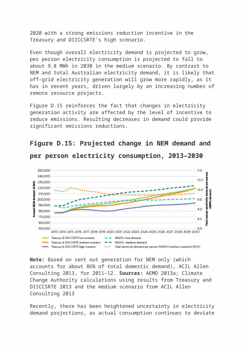
Barriers to energy efficiency and demand management

Potential solutions

the introduction of Standing Council on Energy and Resources-agreed recommendations arising from AEMC’s 2012 Power of Choice review, specifically around incentives for distribution businesses to undertake demand management projects

the introduction of incentives for non-network and network solutions to be considered on a level field.

Sources: Barriers identified in AEMC 2012; Dunstan, Sharpe and Downes 2013; Garnaut 2008; PC 2005 and 2013; Prime Minister’s Task Group on Energy Efficiency 2010

There is considerable consensus about the solutions set out in Table D.5, but implementation has not yet occurred. Despite the in-principle commitment by the Council of Australian Governments (COAG) to remove retail price caps, roll out interval meters nationally and introduce more cost-reflective pricing, progress has been slow. Without these core actions, consumers cannot make the best choices about how they use electricity and manage spending, and third parties are constrained in identifying investments in energy efficiency and demand management with the greatest benefits.

In the near term, the Authority supports additional action that will help increase the uptake of energy efficiency opportunities by consumers, suppliers and energy service companies. Building and equipment choices lock in higher or lower emissions for many years; as stock is renewed, it is important that it is replaced with efficient options to capture the available emissions reduction opportunities.

In addition, priorities could include initiatives that have been identified in previous reviews, including:

collecting and publishing more detailed electricity consumption data, particularly related to end use within buildings, where there are positive net benefits for consumers

completing retail competition reviews and removing retail price regulation where effective retail competition exists

the Australian Energy Regulator implementing standard regulatory arrangements for interval meters

proceeding with the rollout of interval meters for new connections and replacements

where possible, accelerating the response time of AEMC to rule change requests arising from independent reviews, including the SCER and PC.

D3.6 Challenges to tracking progress in the electricity sector

The Authority considers that the best common measure of electricity activity is electricity ‘sent out’, but historical data (to 1990) is not available on this basis in a disaggregated, rigorous form. In order to compare historical and projected activity data, the Authority has used electricity ‘as generated’. ‘Sent out’ electricity leaves the power station, ‘as generated’ includes electricity consumed by the power station itself in its own operations.

The major drivers of reduced electricity demand are known but their relative contribution to changing demand is unclear. More detailed, consistent time series information on end-use electricity consumption could help these drivers be better understood, allowing for improved demand projections and more effective policy design.

Information gaps also make it difficult to track progress in off-grid electricity generation. Off-grid electricity accounts for about 6 per cent of Australia’s electricity generation, and is mainly consumed by the mining and manufacturing sectors (ABS 2012). The level and mix of off-grid generation is a source of uncertainty because granular data is not collected routinely or systematically.

BREE’s inaugural report (2013c) on regional and remote electricity is a welcome source of new information. BREE ‘intends to report on the demand and supply of electricity in off-grid Australia on a regular basis’ (2013c, p. 40). The Authority endorses this plan. Detailed reporting of off-grid generation will inform policy, planning and private investment. It could also aid planning for the potential implications of a shift from gas, which is currently the dominant fuel, and identify opportunities to deploy lower emissions generation over time (ACIL Allen Consulting 2013; ABS 2012).

Appendix D4 Transport

D4.1 Transport emissions overview

Transport greenhouse gas emissions are produced by vehicles combusting fuels to move people and freight. Australia’s transport emissions are reported across four modes—road, rail, domestic aviation and domestic shipping. International aviation and shipping emissions are excluded from Australia’s national inventory. Emissions associated with producing and refining liquid and gaseous fuels, as well as generating electricity, are attributed to stationary energy and fugitives sectors.

Transport accounted for 91 Mt CO2-e (15 per cent) of Australia’s emissions in 2012. Under the medium scenario, transport is projected to account for a similar proportion of total emissions in 2020, reducing to 14 per cent in 2030, as shown in Figure D.16.

Australia’s per capita transport emissions are higher than those of most other countries (IEA 2013a, p. 106). Australia’s urban form, low population density and long intercity distances make it heavily reliant on road transport and domestic aviation. To the extent that these factors are fixed, most of the Australian population and business will continue to depend on these transport modes.

Figure D.16: Transport share of Australia’s emissions, selected

years, 1990–2030

 

Source: Climate Change Authority calculations using results from Treasury and DIICCSRTE 2013

Figure D.17: Passenger road transport activity and emissions

intensity—modelled range, 1990–2050

 

Note: Upper and lower line bounds illustrate range of modelled outcomes. Source: Climate Change Authority calculations using results from Treasury and DIICCSRTE 2013 and Reedman and Graham 2013a

Figure D.18: Passenger road transport activity and emissions

intensity—four scenarios, 1990–2050

 

Source: Climate Change Authority calculations using results from Treasury and DIICCSRTE 2013 and Reedman and Graham 2013a

In all scenarios modelled by the Treasury and DIICCSRTE (2013), considerable growth in road and aviation activity is projected. Passenger road transport activity is expected to increase substantially from about 179 billion to 290 billion vehicle kilometres between now and 2050 (Figure D.17).

Under scenarios with a price incentive, the emissions intensity of passenger road transport is projected to decline significantly between now and 2030, and eventually stabilise between 2040 and 2050, as shown in Figure D.18.

Beyond 2035, however, emissions intensity improvements are not expected to offset growth in the transport task, resulting in growing transport emissions. Continuing growth in activity is estimated to drive up transport emissions to between 97 and 127 Mt CO2-e in 2050, as presented in Figure D.19. This is higher than the 2000 level of 75 Mt CO2-e in all scenarios.

D4.2 Transport emissions outcomes, contributors and drivers

Figure D.19: Contributors to transport emissions, selected years,

1990–2050, and to change in emissions relative to 2000 levels

 

Source: Climate Change Authority calculations using results from Treasury and DIICCSRTE 2013 and Reedman and Graham 2013a

Demand for transport is driven by population growth, economic activity and costs associated with travel (DCCEE 2012, p. 25).

Road transport accounted for 77 Mt CO2-e (84 per cent) of all transport emissions in 2012. This includes light vehicles (motorcycles, cars and light commercial vehicles) and heavy vehicles (rigid and articulated trucks and buses). Light vehicles accounted for 57 Mt CO2-e (63 per cent) of total transport emissions and 10 per cent of Australia’s economy-wide emissions. Passenger vehicles accounted for most of the transport task and, as a consequence, are the largest contributor to emissions, as represented in Figure D.20. Australia’s per capita light vehicle ownership and use is stabilising, making population growth a dominant driver for future growth in passenger road transport.

Road freight is the second-largest contributor to emissions. It includes a diverse range of activities, such as freight hauled between cities by large articulated trucks, transport of goods between retail and distribution

centres, and point-to-point courier movements. The road freight task is growing quickly—between 2001 and 2009, it grew by 37 per cent, from 139 billion tonne-kilometres to 191 billion tonne-kilometres (BITRE 2012, p. 49), driven by increased wealth and economic activity.

Domestic aviation activity, dominated by passenger transport, increased by 80 per cent between 2001 and 2011 (BITRE 2012, p. 89) and is projected to approximately double from 2011 levels by 2030 (DCCEE 2012, p. 15). This strong growth in domestic aviation has been largely driven by broader economic growth and increasing passenger preference for air travel over road or rail. Most classes of air travel have become more affordable—real costs of business, restricted economy and discount airfares have fallen, while real median and average incomes have increased (BITRE 2013 and PC 2013, p. 60). Domestic aviation accounts for more than half of non-road transport emissions (8 Mt CO2-e) and emissions from rail and domestic shipping each account for about 3 Mt CO2-e (Treasury and DIICCSRTE 2013).

In the Treasury and DIICCSRTE (2013) modelling, price incentives apply to only a minority of transport emissions, including those from heavy on-road vehicles from 2014–15. Incentives for light vehicle emissions reduction are not modelled. Emissions from light vehicles are, however, influenced by the incentives applied to other subsectors, which may lead to spillovers of technology improvements and use of lower emissions fuels.

The largest modelled contributors to emissions reduction in transport relate to vehicle efficiency improvements, vehicle electrification and the uptake of low-emission fuels, including sustainable biofuels, in road passenger and freight. These are reflected in Figure D.19.

Vehicle emissions intensity, expressed in grams of CO2 per kilometre (g CO2/km), serves as a robust proxy for vehicle efficiency across conventional fuel types. The emissions intensity of new light road vehicles (including light commercial vehicles) sold in Australia has improved by 21 per cent from 252 g CO2/km in 2002 to 199 g CO2/km in 2012 (NTC 2013, p. 5). This has been driven by technology advances and consumer preferences. Continued improvement is projected to reduce the transport emissions intensity of new vehicles to 2050 in all scenarios.

The projected uptake of electric road vehicles, already underway but expected primarily after 2020, also contributes to the reduction of transport emissions. The emissions attributable to electric vehicles will depend on the source of the electricity, so net emissions reduction from vehicle electrification will depend on the emissions intensity of the electricity supply (Garnaut 2008, p. 519). In 2050, electric road vehicles

are projected to deliver a transport sector emissions reduction of between 2 Mt CO2-e and 6 Mt CO2-e per annum under the low and high scenarios, respectively, compared to the no price scenario.

The broad adoption of lower emission fuels, notably sustainable biofuels, could reduce transport emissions. Under the low and high scenarios, respectively, biofuels are projected to provide 10–20 per cent of Australia’s road transport fuel needs by 2030, resulting in an emissions reduction of between 2 and 8 Mt CO2-e per annum over 2000 levels, compared to the no price scenario.

D4.3 Progress in transport emissions reduction

Broadly, transport emissions can be reduced in three ways:

increasing the efficiency of vehicles, through engine and vehicle technology improvements and take-up of alternative drivetrains in the case of road vehicles

reducing emissions intensity of fuels, through low-emissions alternatives to conventional fuels such as sustainable biofuels and natural gas

making demand management more efficient through mode shift—from road freight to rail or shipping, and from private vehicles to public and active transport—as well as improved urban planning, transport infrastructure, traffic management and intelligent transport systems.

D4.3.1 Increasing the efficiency of vehicles

The CSIRO modelling suggests light vehicle efficiency improvements could offer approximately 18–19 Mt CO2-e of emissions reductions per year by 2050 (Graham et al. 2012b, pp. 40–2). Light vehicle efficiency improvements are expected under a BAU setting, as consumer preferences are influenced by factors such as fuel prices. Improvements can also be significantly increased by regulations on vehicle carbon dioxide emissions.

There are fewer opportunities to reduce heavy vehicle emissions. Projections suggest that, compared to current practice, there is potential to reduce emissions through efficiency gains by up to 5 Mt CO2-e per year by 2050 (Graham et al. 2012b, p. 45). Adoption of low-rolling resistance tyres and regenerative braking systems may offer another 2 Mt CO2-e of cost-effective emissions reductions per year by 2050 (Graham et al. 2012b, p. 46).

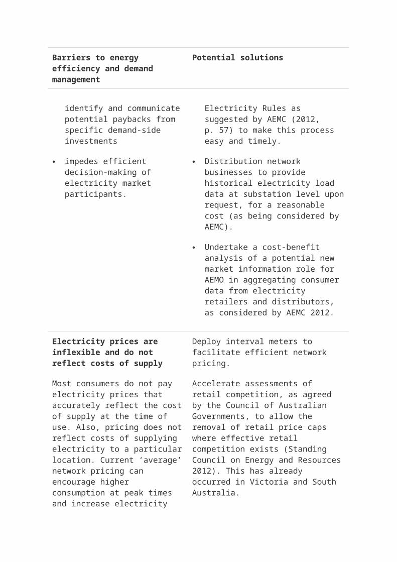
Given the long lifetimes of ships, locomotives and aircraft, there are also fewer opportunities to improve energy efficiency through stock turnover of these vehicles. The largest emissions reduction opportunities for non-road vehicles, compared to current practice, are through technology advances such as engine efficiency and vessel weight, which could reduce transport emissions by about 7 Mt CO2-e per year by 2050 (Graham et al. 2012b, pp. 49, 52 and 54).

By way of comparison, domestic aviation and shipping emissions were about 8 Mt CO2-e and 3 Mt CO2-e, respectively, in 2012.

Vehicle electrification

Road vehicle electrification, combined with a decarbonised electricity sector, offers substantial emissions reduction potential. Vehicles need not be fully electric—there are various degrees of electrification, such as stand-alone hybrid electric vehicles (HEVs) and plug-in hybrid electric vehicles (PHEVs).

The emissions of purely electric vehicles (EVs) and PHEVs—when operating in full electric mode—are represented in the electricity sector rather than transport. Their fuel cycle emissions intensity compared to internal combustion engine vehicles (ICEVs) and HEVs depends on the emissions intensity of the electricity grid and relative vehicle efficiencies. Typical mass-produced EVs are more than twice as energy efficient as ICEVs.

With a low-emissions electricity supply, the electrification of light and heavy vehicles could offer emissions reductions of between 23 and 25 Mt CO2-e in 2050 (Graham et al. 2012b, pp. 40, 47). One of the current barriers to the take-up of EVs is their high up-front cost compared with ICEVs and HEVs (although operating costs are much lower). Given assumed technology improvements and cost reductions, the cost of owning an EV could reach parity with an ICEV by the late 2020s (Graham et al. 2012a, p. 25).

Fleet-average emissions standards for light vehicles

Despite recent improvements, Australia has not made the same gains as other auto markets in light vehicle fuel efficiency and CO2 emissions. At 190 g CO2/km, on average, light passenger vehicles sold in Australia in 2012 were 44 per cent more emissions-intensive than those sold in the same year in the EU, which averaged 132 g CO2/km (NTC 2013, p. 24; European Environment Agency 2013, p. 3).

Adoption of standards on vehicle fuel efficiency and CO2 emissions has led to improvements in vehicle efficiency worldwide. Regulations and

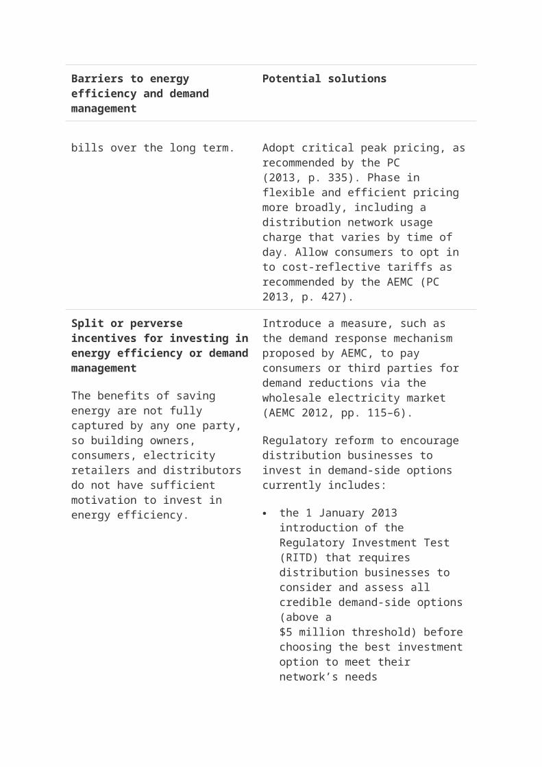
targets intended to significantly improve on BAU outcomes are in place or being established in major markets such as the EU, the US, Canada, China, Japan and South Korea. About three-quarters of light passenger vehicles sold in the world today are subject to regulated CO2 emissions standards or, equivalently, fuel economy standards (see Figure 11.10 in Chapter 11).

The EU has several policies to reduce CO2 emissions from new vehicles, including a fleet-average target of 95 g CO2/km for new light passenger vehicles by 2020, and is considering a target of 73 g CO2/km by 2025 (European Commission 2013). The implied reduction rates under these targets are about 4 per cent per year between now and 2020, and about 5 per cent per year between 2020 and 2025.

The US has implemented standards targeting the fuel economy of light vehicles, with equivalent3 average CO2 intensity targets of 139 g CO2/km by 2020 and 109 g CO2/km by 2025. The implied reduction rates under these targets are about 5 per cent per year between now and 2025.

Figure D.20: Comparison of passenger vehicle CO2 emission rate

projections, 2000–2025

 

Source: Adapted from ICCT 2013 and NTC 2013

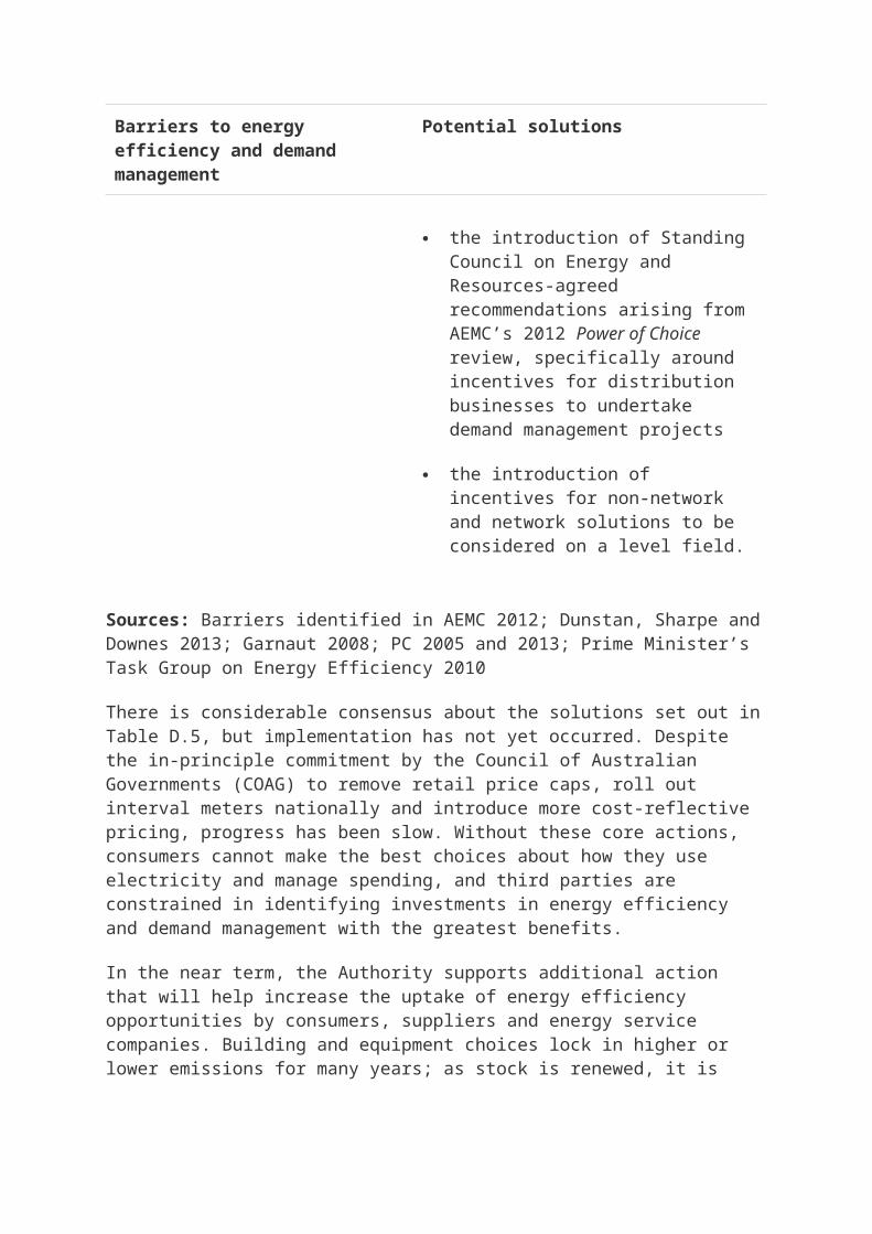
Australia has previously considered adopting fleet-average CO2 emissions standards, and has regulations that require manufacturers and importers to display the fuel consumption and CO2 emissions of new vehicles for sale (DIT 2011). As discussed in Chapter 11, the Authority recommends that the Commonwealth Government investigates implementing fleet-average CO2 emissions standards for Australia.

Although most light vehicles sold in Australia are imported from countries with fuel efficiency standards, there is a risk that Australia will not receive the full benefit of those standards. The most fuel-efficient vehicles and model variants are typically allocated to markets with mandatory standards (DIT 2011, p. 8). If Australia pursued a similar rate of improvement in its fleet-average emissions as that required by the EU 2020 target, new light passenger vehicles sold in Australia in 2020 would be about 20 per cent more efficient than those sold today. Adopting a target comparable to the EU’s (95 g CO2/km by 2020) could reduce the emissions intensity of new light passenger vehicles, on average, to about half of today’s level.

Box D.5: How do fleet-average emissions standards work?

A single fleet-wide target, based on vehicle CO2 emissions intensity, is applied across all new light vehicle sales for a given year. Targets are tightened over time and are designed to drive greater vehicle efficiency improvements than would have occurred under BAU.

The target for individual suppliers is determined according to a mathematical relationship between CO2 emissions and a particular vehicle attribute (usually mass or size). Suppliers can market models above or below the fleet target value applicable to a particular vehicle, as long as the average emissions intensity of all their models sold in a given year meets their target as determined by the mathematical relationship. This approach provides flexibility for suppliers and enables them to choose the most cost-effective technologies to achieve their targets.

A flat target that imposes the same limit on all suppliers is simpler in design but likely to lead to inequities given the different sectors of the market that the various suppliers occupy. Attribute-based standards provide a more equitable distribution of responsibility while still achieving the desired emissions reductions from the fleet overall. Attribute-based targets mean that fleet-average emissions standards do not drive the phase-out of large vehicles if there is a market demand for such vehicles; rather, it places pressure on suppliers to improve the efficiency of their vehicles. Attribute-based targets are applied in other vehicle markets; in the US, standards are set according to average

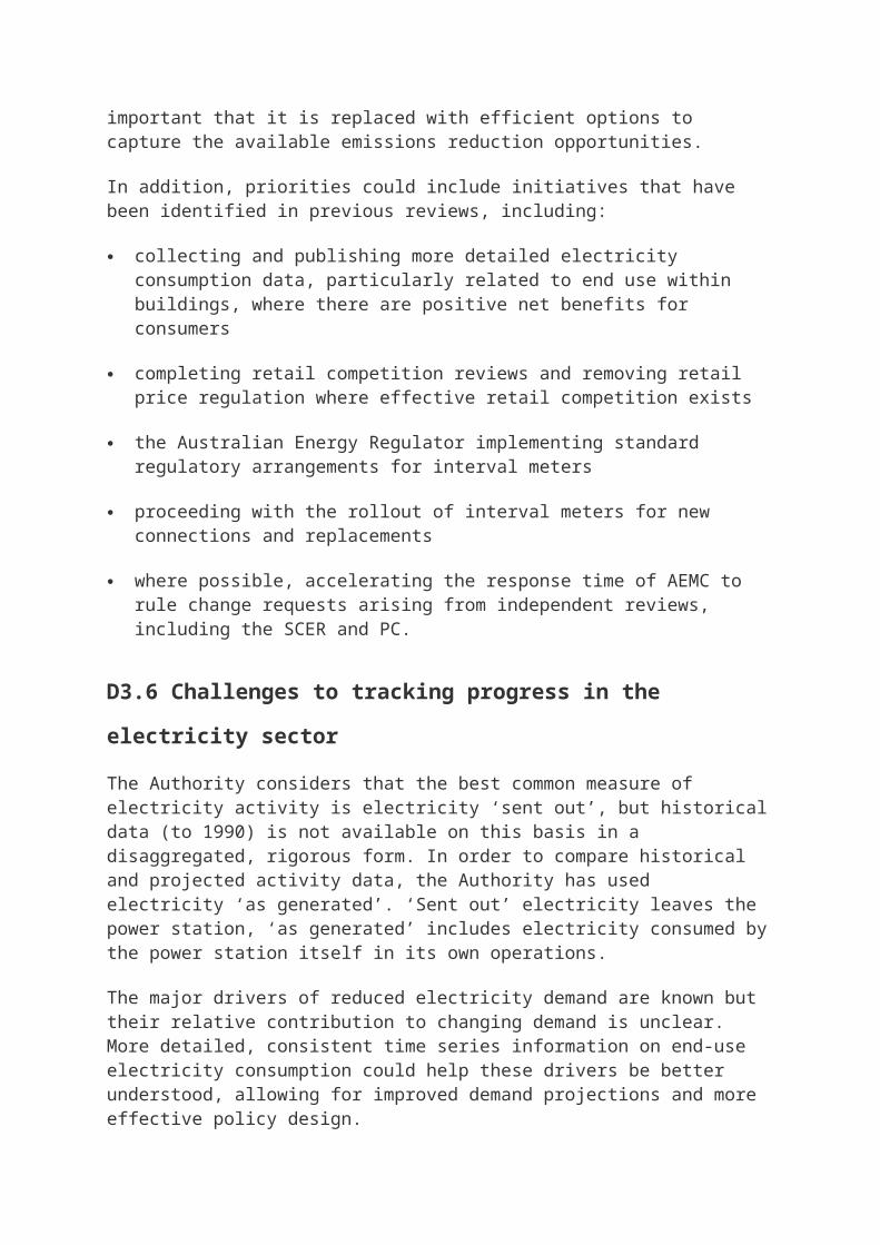
vehicle size (footprint), while in the EU standards are based on average vehicle mass.

The Authority commissioned the CSIRO to model the emissions reduction potential of Australia adopting fleet-average CO2 emissions standards that drive a rate of efficiency improvement comparable to other markets. Improvement over the last decade has been about 2.3 per cent per year on average (NTC 2013, p. 5). The CSIRO modelled lenient, medium and stringent standards, reflected by annual improvement rates of 3.5, 5 and 6.5 per cent respectively.

The CSIRO modelling showed that, by 2030, up to 14 Mt CO2-e per annum (13 per cent of total transport emissions in that year) could be avoided using fleet-average CO2 emission standards introduced in 2018. For the entire modelled period (from now until 2050), introducing relatively lenient standards in 2018 was projected to achieve greater emissions reductions than introducing stringent standards in 2025, emphasising the importance and value of early action in transitioning Australia’s light vehicle fleet to lower emissions vehicles. Figure D.21 shows the cumulative emissions reductions available.

Figure D.21: Cumulative light vehicle emissions reductions with

CO2 emissions standards, compared to BAU projections, 2030–2050

 

Source: Climate Change Authority calculations using results from Treasury and DIICCSRTE 2013 and Reedman and Graham 2013b

CO2 emissions standards could offer net benefits to vehicle owners, as well as public benefits in reducing emissions. Mandatory CO2 emissions standards are considered one of the most cost-effective strategies to reduce transport emissions (DIT 2011, p. 3).

The impact of emissions standards on vehicle costs in Australia will generally be determined by global vehicle markets (Reedman and Graham 2013b, p. 5). As a result, international evidence provides some useful insights for Australia. The Authority considers, based on analysis done in other markets, the overall private cost of vehicle emissions standards for Australia at levels comparable to international action may be negative (that is, delivering net savings)—even after higher vehicle purchase costs are taken into account.

In Europe, for example, under a 2020 target of 95g CO2/km by 2020, the real purchase price of the average car is projected to be €1,100 more. Real fuel costs for the average car, however, will be about €400 less per year (Cambridge Econometrics and Ricardo-AEA 2013, p. 3). In the US, the National Highway Traffic Safety Administration (NHTSA) projects the latest Corporate Average Fuel Economy (CAFE) standards will deliver average net benefits of about US$3,400 (for cars) and US$4,700 (for light trucks) for vehicles manufactured in 2025 (NHTSA 2012, p. 978). These estimates do not take into account the social benefits arising from the reduction in emissions.

Fuel and operating savings, however, are specific to each market. According to CSIRO modelling of standards for Australia, a saving of 4 cents per kilometre is projected by the time the majority of the fleet has been subjected to CO2 standards (after 2035). At about 15,000 km per year travel—typical for Australia—the annual savings are close to $600. This suggests CO2 standards in Australia could give consumers a private return on investment comparable to that in the US or EU.

ClimateWorks (2010, p. 78) suggests that, in Australia to 2020, a standard of 140 g CO2/km could deliver societal savings of up to $74 per tonne of CO2 avoided, and achieve annual emissions reductions of 5.5 Mt CO2, with benefits to the economy of about $400 million. The potential savings increase to $85 per tonne of CO2 for a standard of 120 g CO2/km, which could deliver emissions reductions of 6.3 Mt CO2 and economic benefits of about $535 million.

Standards could have substantial complementary benefits:

Reduced fuel consumption will lower costs and increase transport productivity. CSIRO modelling projects that under a lenient standard starting in 2018, about 161 PJ less transport energy, of all types, will

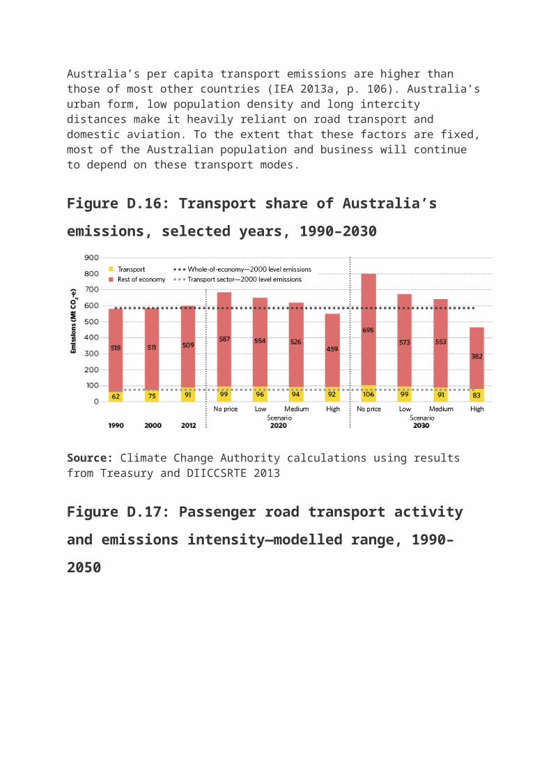
be required in 2030 and about 275 PJ less in 2050. Petroleum consumption alone will be reduced by about 170 PJ per annum by 2050, which decreases Australia’s projected petroleum needs in 2050 by about 5 per cent (BREE 2012, p. 46).

Standards are projected to bring alternative drivetrains, such as plug-in electric vehicles, to Australian roads more quickly, with associated health and amenity benefits from reduced noise and air pollution. CSIRO modelling projects that under a medium standard starting in 2018, over one-quarter of all light vehicle travel will be undertaken by alternative drivetrain vehicles by the early 2040s, compared to about 7 per cent without standards.

Implementing CO2 standards in Australia may be done at relatively low administrative cost. It may require new legislation but is not expected to introduce additional vehicle testing relative to current requirements.

D4.3.2 Reduced emissions intensity of fuels

Oil is the main energy source for transport (IEA 2013b, p. 572). Alternative transport fuels with potentially lower emissions intensity are both available and in development, including liquid biofuels and gaseous fuels. Synthetic fuel alternatives are also in development or are available overseas, including coal-to-liquid, gas-to-liquid and shale oil-to-liquid, most of which could have higher emissions intensity than conventional fuels.

The growth of a low-emission fuels market depends on the cost and availability of these fuels as alternatives. Some modelled scenarios project a significant increase in biofuel use; however, there is a risk that future oil prices and biofuel supply constraints could prompt Australia to exploit fuels that have higher lifecycle emissions, in order to meet its transport fuel needs. Improving vehicle efficiency and electrification of transport mitigates this risk.

Natural gas may increase its share of the transport fuels mix; however, it is likely to depend on the relative pricing of natural gas to alternatives. Liquefied petroleum gas is not projected to gain significant future additional market share for road vehicles or locomotives; however, future prices of alternatives may change this outlook.

Biofuels

Biofuels are considered zero-carbon under international accounting standards but, depending on the feedstock, the upstream emissions associated with producing biofuels can be higher than for fossil fuels (PC 2011, p. 7). In Australia, however, even after lifecycle process emissions

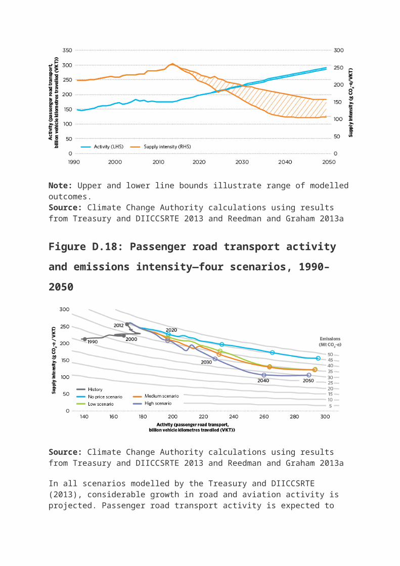
are taken into account, biofuels are lower in emissions intensity than fossil-derived fuels (Figure D.22).

Figure D.22: Upstream and downstream emissions of diesel fuels

 

Note: Representative of a truck consuming 10 MJ/km of fuel energy (Beer et al. 2007, p. 50).Source: Adapted from Beer et al. 2007, p. 92

The potential of biofuels may be limited by the availability of appropriate feedstock. First-generation or conventional biofuels are produced from grain-based feedstocks. Second-generation biofuels (including Australian biofuels) are produced from waste materials and co-products of food production, reducing the potential for food displacement or other unsustainable environmental outcomes. A newer second-generation biofuel—algal biofuel—produced from algae that can be grown in water bodies such as waste streams or the ocean, has the potential to be a sustainable alternative to conventional diesel. Algal biofuel is currently in the research and development stage and not yet commercially available (CSIRO 2013). Increased use of biofuels may diminish the emissions reduction potential of improved vehicle efficiency; however, this effect is limited by the availability of appropriate feedstock. Ultimately, both biofuels and efficient vehicles could help reduce Australia’s emissions and its reliance on petroleum imports.

With a price incentive, adopting sustainable biofuels for road transport could reduce annual emissions by up to 3 Mt CO2-e per year by 2050. Increased biofuel use could diminish the potential for emissions reductions from vehicle electrification and vice versa.

For rail and domestic shipping, the use of biofuels could offer the largest emissions reduction opportunity, totalling 2–4 Mt CO2-e per year by 2050 (Graham et al. 2012b, pp. 53, 55). This is also the case for domestic aviation, where biofuels have the potential to reduce emissions by 6 Mt CO2-e in 2050 (Graham et al. 2012b, p. 50).

Current supply of feedstock in Australia is not expected to be enough to meet substantial increases in demand (Wild 2011), and other potential sources may be favoured to supply a growing market for biofuels.

Regulatory drivers, such as New South Wales’s biofuel mandates, can support increased biofuel use, but may not guarantee the biofuel is produced sustainably.

D4.3.3 More efficient demand management and mode shifts

There is potential for emissions reductions through mode shifts from road freight to rail and shipping. Based on international research, rail and shipping offer lower emissions intensity transport, at an average of 23 g CO2 per tonne-km and 5–13 g CO2 per tonne-km, respectively. By comparison, road freight averages 120 g CO2 per tonne-km (Cristea et al. 2011, p. 38). Coupled with improved freight logistics, mode shift could reduce freight emissions by up to 5 Mt CO2-e per year by 2050 (Graham et al. 2012b, p. 82).

Rail is the primary mode to move bulk freight, such as coal and iron ore. It plays less of a role in moving other freight, where its share, compared with long-haul road vehicles, is less than 10 per cent in the two largest corridors—between Sydney and Melbourne, and Sydney and Brisbane (BITRE 2009, p. 6). Investment in road infrastructure has brought more time-efficient and cost-effective road freight along these commercial routes. Rail becomes cost-competitive with road over distances longer than 1,000 kilometres, but transit time increases at a higher rate than for road freight (BITRE 2009, p. 8). Investment in rail infrastructure along these corridors could reduce transit time and costs, and improve rail’s share of freight transport. However, there are long timeframes for investment and payback, which are a barrier to a broader uptake of rail freight transport.

Passenger mode shift from private vehicles to public and active transport also offers emissions reduction opportunities, with options ranging from increased use of public transport infrastructure to measures that encourage cycling and walking. It is estimated that switching from private car to other transport modes could offer emissions reductions of up to 7 Mt CO2-e per year by 2050 (Graham et al. 2012b, pp. 69, 70, 72).

Australia’s cities are more sparsely populated than most cities of the world (DIT 2013, p. 112), which presents a challenge to broader use of public and active transport. The potential for passenger mode shift is difficult to quantify—users’ mode selection depends on the alternative transport options available and, potentially, policies and programs that influence travel behaviour change.

Emissions reductions could also be achieved through intelligent transport systems (ITS). ITS comprise a range of information and communications technologies that can be applied to optimise travel patterns, including traffic management. It is estimated that, if adopted, intelligent traffic management could reduce emissions by about 3 Mt CO2-e per year by 2050 (Graham et al. 2012b, p. 80). Austroads, the association of Australian and New Zealand traffic authorities, is developing an ITS architecture to facilitate consistent and interoperable ITS delivery. The project, which is scheduled to be completed in 2016, will establish the regulatory and operational framework for ITS in Australia (Austroads 2013).

Appendix D5 Direct combustion

D5.1 Direct combustion emissions overview

Direct combustion is burning fuels for stationary energy purposes, such as generating heat, steam or pressure. It excludes fuels combusted for electricity generation.

Australia’s direct combustion emissions were 75 Mt CO2-e in 2000 and 95 Mt CO2-e in 2012. This represented 13 per cent and 16 per cent of total Australian emissions in 2000 and 2012.

The oil and gas industries, metal manufacturing and households are large contributors to direct combustion emissions. The balance of emissions can be attributed to other industrial and commercial use.

Figure D.23: Direct combustion share of Australia’s emissions,

selected years, 1990–2030

 

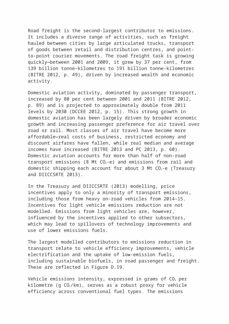
Source: Climate Change Authority calculations using results from Treasury and DIICCSRTE 2013

Australia’s rapidly expanding LNG industry is expected to be the main contributor to direct combustion emissions growth, particularly in the next few years. By 2020, direct combustion emissions are projected to be 49–59 per cent higher than 2000 levels, and 57–79 per cent higher by 2030 (Figure D.23).

From 2012 to 2030, direct combustion is projected to be responsible for the largest absolute increase in emissions in any sector of the Australian economy—driven primarily by LNG production—except under the no price scenario.

Emissions levels are closely correlated with the total energy content of fuel combusted. Direct combustion emissions intensity improved moderately between 2000 and 2012; a trend projected to continue across all scenarios to 2030 (figures D.24 and D.25), as natural gas takes an increasing share of the total primary energy mix.

Figure D.24: Direct combustion activity and emissions intensity,

1990–2030

 

Note: Upper and lower line bounds illustrate the range of modelled outcomes.Source: Climate Change Authority calculations using results from Treasury and DIICCSRTE 2013

Figure D.25: Historical and projected direct combustion activity

and emissions intensity, 1990–2030

 

Source: Climate Change Authority calculations using results from Treasury and DIICCSRTE 2013

D5.2 Direct combustion emissions outcomes, contributors and drivers

Direct combustion emissions from LNG production relate to onsite use of natural gas to fuel stationary equipment, particularly the compression turbines used to liquefy natural gas. Figure D.26 shows the modelled impact of price incentives on direct combustion emissions. All scenarios show strong emissions growth to 2020—the lowest projection in 2020 is almost 50 per cent higher than 2000 levels. The opportunity for emissions reductions, regardless of the level of incentive, is somewhat limited by long-term supply contracts in the growing LNG industry. While LNG exports totalled 24 million tonnes in 2012 (BREE 2013a, p. 24), there is over 114 million tonnes of annual LNG production capacity in operation, under construction or at initial stages in Australia (BREE 2013a, pp. 32–33) (Table D.6).

Figure D.26: Contributors to direct combustion emissions, selected

years, 1990–2030, and to change in emissions relative to 2000 levels

 

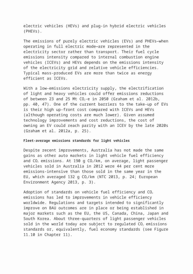
Source: Climate Change Authority calculations using results from Treasury and DIICCSRTE 2013

Table D.6: Australian LNG projects

Existing Capacity (million tonnes/year)

Completion

North West Shelf (WA) 16.3 Operating

Pluto (WA) 4.3 Operating

Darwin LNG (NT) 3.7 Operating

Under construction Capacity (million tonnes/year)

Completion

Gorgon (WA) 15.6 2015

Australia Pacific LNG (Qld)

9.0 2015

Wheatstone (WA) 8.9 2016

Queensland Curtis LNG (Qld)

8.5 2014

Ichthys (NT) 8.4 2017

Gladstone LNG (Qld) 7.8 2015

Prelude Floating LNG (WA)

3.6 2017

Feasibility stage Capacity (million tonnes/year)

Completion

Scarborough Floating LNG (WA)

6.0 2018+

Gorgon LNG Train 4 (WA) 5.2 2018+

Bonaparte Floating LNG (NT)

3.0 2018+

Browse Floating LNG (WA)

N/A 2018+

Proposed Capacity (million tonnes/year)

Completion

Arrow LNG (Qld) 8.0 2017+

Sunrise (NT) 4.0+ 2017+

Cash Maple (NT) 2.0 2018+

Equus (WA) N/A 2018+

Source: BREE 2013a

More generally across the industrial, residential and commercial sectors, energy efficiency is likely to play an increasingly important role across all forms of direct combustion, somewhat constraining growth in emissions.

D5.3 Progress in direct combustion emissions reduction

D5.3.1 Natural gas industry

The projected increase in direct combustion emissions results from large increases in LNG exports and limited opportunities to improve the emissions intensity of LNG production. Demand for Australian fossil fuel exports such as LNG is driven by global commodity prices and the exchange rate, as well as global and regional economic growth.

Improvements in emissions intensity may come from energy efficiency gains in turbines and other machinery. Australia Pacific LNG (2010, p. 25) notes that the most fuel-efficient turbines result in approximately 25 per cent less greenhouse gas emissions compared with commonly used turbines around the world. Additionally, heat captured from a gas turbine’s exhaust may be used in the LNG liquefaction process to augment gas-fired boilers.

D5.3.2 Alumina refining

Non-ferrous metal manufacturing, principally alumina refining, is the second-largest source of direct combustion emissions.

Between 2005 and 2012, direct combustion emissions from alumina refining stayed at about 8 Mt CO2-e (Treasury and DIICCSRTE 2013), despite a 21 per cent increase in alumina production (BREE 2013b). This improvement in emissions intensity is largely due to fuel-switching from coal to gas.

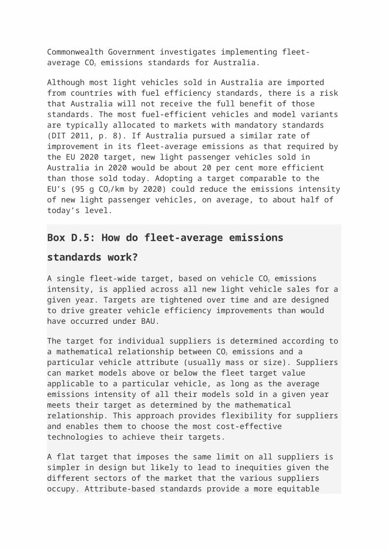
Between 2012 and 2020, direct combustion emissions from alumina refining are projected to increase by 18 per cent to 10 Mt CO2-e (Treasury and DIICCSRTE 2013) as production increases (BREE 2012b, p. 48). Further improvement in emissions intensity may come from process refinements. Opportunities vary, from co-generation plants, whose waste heat can generate steam for use in the alumina refining process (DRET 2008, p. 8), to systems optimisation, which more efficiently controls the use of natural gas (DRET 2013, p. 2). Absolute emissions reductions, or large gains in emissions intensity, may be limited unless fossil fuel combustion is replaced by lower emissions sources (DCCEE 2012, p. 14).

D5.3.3 Residential sector

Continued regulatory improvements to the thermal efficiency of residential homes and the energy efficiency of household appliances, such as hot water systems, could represent significant emissions reduction opportunities. George Wilkenfeld and Associates (2009, p. 40) project that equipment energy efficiency standards affecting residential gas use may save 4.5 Mt CO2-e between 2000 and 2020. There may be an increase in sectoral emissions, however, as conventional electric resistive water heaters are phased out. The effect on direct combustion emissions will depend on householders’ preferences for gas, solar or heat pump water heaters, and choices between gas and electric heat pump space heating. The overall effect on emissions will also depend on the emissions intensity of electricity generation and the relative improvements in appliance efficiency.

Appendix D6 Fugitive emissions

D6.1 Fugitive emissions overview

Fugitive emissions are greenhouse gases emitted during the extraction, production, processing, storage, transmission and distribution of fossil fuels such as coal, oil and gas. Fugitive emissions do not include emissions from fuel combustion.

Australia’s fugitive emissions were 41 Mt CO2-e in 2000 and increased to 48 Mt CO2-e in 2012 (Treasury and DIICCSRTE 2013). This represented 7 and 8 per cent of Australia’s total emissions in 2000 and 2012, respectively (Figure D.27). Almost three-quarters of 2012 fugitive emissions were from the coal industry, with the balance from the oil and gas industry.

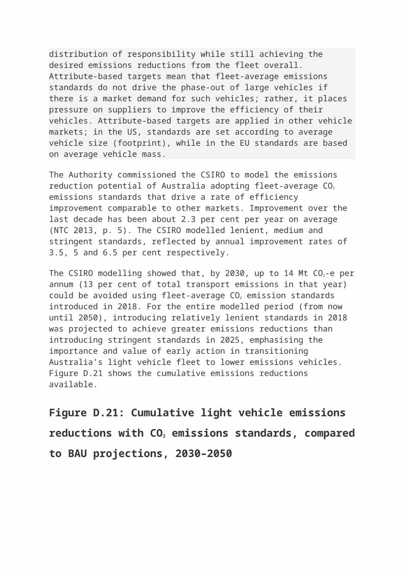
The Treasury and DIICCSRTE modelling (2013) projects fugitive emissions will increase relative to 2000 levels by 2030 under all scenarios. Growth ranges from an 8 Mt CO2-e to 59 Mt CO2-e increase under the high and no price scenarios, respectively (Figure D.27). The projected increase reflects growth in coal and LNG production, driven by strong global demand for Australia’s energy resources. The scenarios project a wide range of possible future fugitive emissions levels in 2030 (Figure D.28).

Figure D.27: Fugitive share of Australia’s emissions, selected years,

1990–2030

 

Source: Climate Change Authority calculations using results from Treasury and DIICCSRTE 2013

Figure D.28: Historical and projected fugitive emissions, 1990–2030

 

Note: Upper and lower line bounds illustrate the range of modelled outcomes.Source: Climate Change Authority calculations using results from Treasury and DIICCSRTE 2013

D6.2 Fugitive emissions outcomes, contributors and drivers

Figure D.29 shows the projected fugitive emissions outcomes for each modelled scenario. All scenarios project a steep increase in emissions to 2020, but diverge in the decade post-2020. By 2030, emissions are projected to be 21 per cent above 2000 levels in the high scenario and 144 per cent above in the no price scenario. This reflects the potential for strong incentives to enhance the economic attractiveness of emerging emissions reduction processes, such as the oxidisation of ventilation air methane in coal mining.

Future fugitive emissions are projected to be driven by growing coal and gas production in response to increased global energy demand. If there is increased global action on climate change, production of fossil fuels (particularly coal) is projected to grow at a slower rate (Treasury and DIICCSRTE 2013). This effect is incorporated in all the scenarios modelled and is most pronounced in the high scenario.

D6.2.1 Coal industry

Fugitive emissions in the coal industry depend on the level of coal production and the greenhouse gas content of the coal seams being mined. ClimateWorks (2013, p. 36) notes that some of the more emissions-intensive mines generate up to 0.8 t CO2-e of fugitive emissions per tonne of coal produced.

Underground mines are typically more emissions-intensive than surface mines because deeper coal seams are subject to greater pressures, which prevents the natural escape of emissions through cracks and fissures (US EPA 2006a, p. 1). In Australia, underground coal mines are around seven times more emissions-intensive than surface mines on average—they contributed 19 per cent to Australian coal production in 2010–11 but 62 per cent of coal fugitive emissions (DCCEE 2012).

Between 2000 and 2012, Australia’s raw coal production increased by 36 per cent (BREE 2013b), while fugitive emissions from coal increased by 24 per cent (Treasury and DIICCSRTE 2013), suggesting improved emissions intensity.

Although price incentives for emissions reduction are projected to affect the emissions intensity of production, growth in Australia’s fugitive emissions will continue to be driven largely by global demand for Australian coal. For example, BREE (2012, pp. 36, 51) projects total black coal production to increase from 11,700 PJ in 2012–13 to 18,000 PJ in 2049–50, and domestic black coal consumption to decrease from 1,200 PJ to 478 PJ.

Figure D.29: Contributors to fugitive emissions, selected years,

1990–2030, and to change in emissions relative to 2000 levels

 

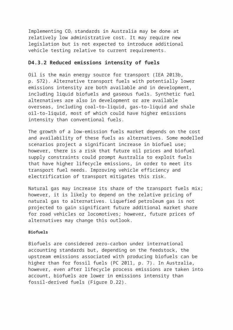
Source: Climate Change Authority calculations using results from Treasury and DIICCSRTE 2013

D6.2.2 Oil and gas industry

Fugitive emissions in the gas industry include gas venting, gas flaring and losses associated with the transmission and distribution of gas.

Between 2000 and 2012, fugitive emissions from natural gas production decreased 18 per cent and emissions from natural gas transmission and distribution increased by 55 per cent (Treasury and DIICCSRTE 2013). Overall, fugitive emissions from the gas industry remained steady over the period, despite natural gas (and ethane) production doubling between 2000 and 2012 (BREE 2013b). Oil production decreased over this period; however, its relatively small contribution to emissions means it is not driving changes in emissions.

The Grattan Institute (2013, p. 4) identifies several trends driving increased demand for gas, including:

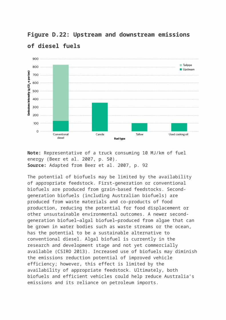
economic growth in China, India and the Middle East, leading to increased energy demand generally

several countries changing their policies on nuclear power, notably Australia’s major trading partner Japan, following the Fukushima nuclear incident, leading to increased demand for alternative energy sources

climate change concerns making gas-fired power plants more attractive, as they emit less greenhouse gases than coal-fired power plants.

These factors contribute to a strong growth outlook—Australian gas production is projected to increase by 184 per cent between 2012–13 and 2049–50 (BREE 2012), considerably larger than the growth in domestic consumption.

D6.3 Progress in fugitive emissions reduction

D6.3.1 Coal industry

There are several emissions reduction technologies the coal industry could use to reduce fugitive emissions, though their implementation may require a price incentive or technological maturation. The US EPA (2006a, p. 2) identified three main measures:

degasification to capture methane

enhanced degasification to capture low-grade methane and purify it

oxidisation of ventilation air methane (when methane in a mine’s ventilation air is oxidised to generate heat or produce electricity).

A price incentive could encourage uptake of these technologies. For example, ClimateWorks (2013) estimates reducing emissions from ventilation air methane oxidisation costs about $17/t CO2-e. A price incentive could also drive a shift in Australian coal production towards less gassy mines.

The level of coal mining activity will be the main driver of fugitive emissions. The Treasury and DIICCSRTE (2013) suggests Australia’s coal production level will be more responsive to global action to reduce emissions than to Australia’s domestic price incentive. With strong global action on climate change, domestic coal production is projected to be flat from 2020 before falling towards the end of that decade. With weaker action, Australia’s production is projected to continue to grow.

D6.3.2Oil and gas industry

The US EPA (2006b, p. 2) identified three main fugitive emissions reduction measures for the natural gas industry:

Equipment changes and upgrades—including pneumatic control devices, which operate valves and control pressure, flow or liquid levels. These devices can be retrofitted or replaced to ‘bleed’ less natural gas into the atmosphere, or used with compressed air instead of pressurised natural gas (Copenhagen Consensus on Climate 2009, p. 22).

Changes in operational practices—including avoiding the venting of methane before pipeline maintenance or repairs. This may mean recompressing the gas during maintenance and repairs or using surge vessels, which clear the pipeline of methane for short periods (Ecofys 2009, p. 27).

Direct inspection and maintenance—including identifying and addressing leaks across the natural gas transmission and distribution network. Infrared cameras can find methane emissions and, if coupled with emissions measurement technologies such as pressure sensors, allow leaks to be tracked and rectified (Clean Air Task Force 2009, p. 16).

CCS could significantly reduce fugitive emissions from oil and gas extraction and processing, though it is not yet widespread (IEA 2013, p. 19). The Gorgon LNG project in Western Australia is expected to capture and inject as much as 3.4 Mt CO2 annually from 2015 (Chevron 2013). Queensland LNG projects are unlikely to use CCS.

The demonstrated reserves of coal seam gas (CSG) in Australia are substantial and estimated to be 31 per cent of Australia’s gas resources (BREE 2013a), with deposits concentrated in Queensland and New South Wales. The CSIRO and Department of the Environment are undertaking a project to gather preliminary field measurements of fugitive emissions from CSG. This is a first step to establishing methods for assessing Australia-specific fugitive emissions from CSG (CSIRO 2013).

Appendix D7 Industrial processes

D7.1 Industrial process emissions overview

The main sources of industrial process emissions are:

metal production in iron, steel and aluminium products

synthetic greenhouse gases from refrigeration and air conditioning use

chemical processes in fertiliser and explosives manufacturing

mineral production, primarily in the cement industry.

Industrial process emissions exclude energy-related emissions such as the burning of fossil fuels for electricity, heat, steam or pressure. These emissions are attributed to electricity, direct combustion or transport.

Australia’s industrial process emissions accounted for 32 Mt CO2-e (5 per cent) of Australia’s emissions in 2012 (Figure D.30).

Figure D.30: Industrial process share of Australia’s emissions,

selected years, 1990–2030

 

Source: Climate Change Authority calculations using results from Treasury and DIICCSRTE 2013

From 1990 to 2012, industrial process emissions increased by almost 7 Mt CO2-e, due to increased use of synthetic greenhouse gases and growing chemical production. This was partly offset by lower metal production and improved metal processing.

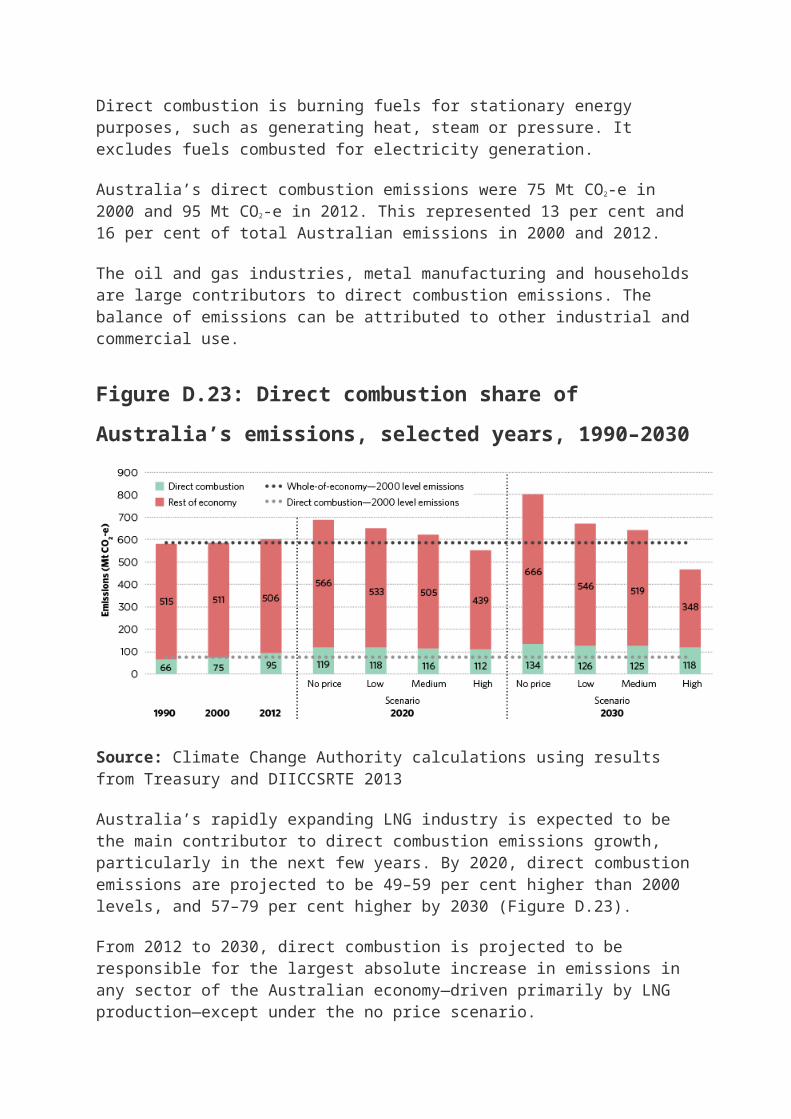
In 2012, industrial process emissions comprised metal production (37 per cent), synthetic greenhouse gases (27 per cent), chemical processing (19 per cent), mineral production (15 per cent) and other production (2 per cent).

The Treasury and DIICCSRTE modelling projects industrial process emissions to be lower, relative to 2000 levels, by 2–4 Mt CO2-e in 2030 under the low and medium scenarios, respectively, and by 15 Mt CO2-e (59 per cent) under the high scenario. Emissions are reduced through improved chemical processing and the transition to alternative refrigerant gases.

Figure D.31: Process emissions from metal production, synthetic

greenhouse gases and other production, 1990–2030

 

Note: Upper and lower line bounds illustrate the range of modelled outcomes. Source: Climate Change Authority calculations using results from Treasury and DIICCSRTE 2013

Figure D.32: Process emissions from chemical and mineral

production, 1990–2030

 

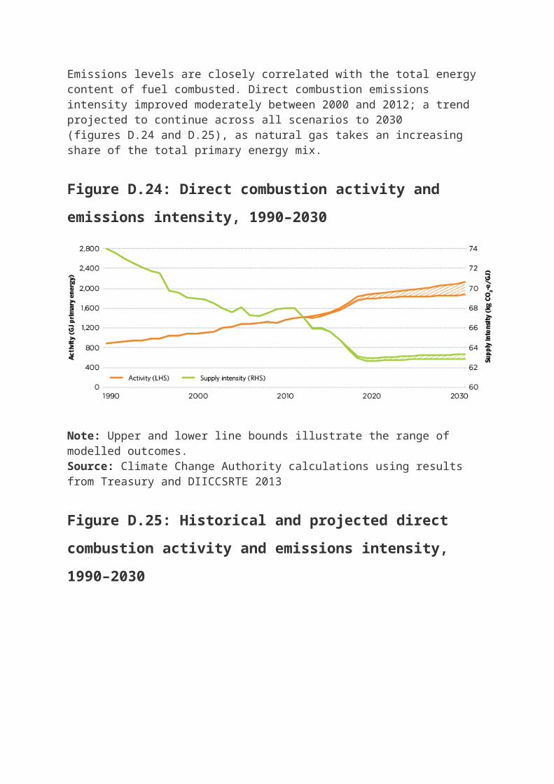
Note: Upper and lower line bounds illustrate the range of modelled outcomes.Source: Climate Change Authority calculations using results from Treasury and DIICCSRTE 2013

Figure D.33: Contributors to industrial process emissions, selected

years, 1990–2030, and to change in emissions levels relative to 2000

levels

 

Source: Climate Change Authority calculations using results from Treasury and DIICCSRTE 2013

D7.2 Industrial process emissions outcomes, contributors and drivers

The majority of the projected emissions reduction in 2030 results from installing nitrous oxide conversion catalysts, recovering and destroying synthetic greenhouse gases, and replacing ozone-depleting substances and refrigerants with lower emitting alternatives. Metals and minerals processing emissions are projected to decline with a price incentive.

Nitrous oxide conversion catalysts offer substantial emissions reduction opportunities, particularly in the context of growing chemical production. Ammonia production emissions are expected to increase in line with expanding explosives production for use in the mining sector and growing demand for fertilisers as the agriculture sector continues to recover from prolonged drought (IBISWorld 2013, p. 9). Planned projects would increase current ammonium nitrate production capacity by over

60 per cent to 1,300 kilotonnes per annum by 2020 (ClimateWorks 2013, p. 49).

ClimateWorks (2013, p. 49) estimates nitrous oxide conversion catalysts could lower nitric acid emissions intensity by 44 per cent in 2020. The cost of conversion catalysts means that incentives or regulation may be needed to drive broad adoption.

According to the Treasury and DIICCSRTE modelling, between 2012 and 2020, synthetic greenhouse gas emissions (used as propellants and refrigerants) are projected to decrease by about 2 Mt CO2-e under the medium scenario and 4 Mt CO2-e under the high scenario. Moving to less emissions-intensive refrigerant gases could deliver a further 6 Mt CO2-e of emissions reduction by 2020.

Metal production emissions decreased by 4 Mt CO2-e to 12 Mt CO2-e between 1990 and 2012, as a result of reduced iron and steel production and improved metal processing. In particular, aluminium emissions intensity fell by over 60 per cent between 1990 and 2011 due to reductions in perfluorocarbon (PFC) emissions. PFC reduction opportunities have been largely taken up; only 20 grams of PFC were emitted per tonne of aluminium produced in 2011, compared with over 450 grams in 1990 (DIICCSRTE 2013, p. 168).

Metal production has contracted recently, as a result of the closure of one of Bluescope Steel’s Port Kembla steelworks in 2011 and Norsk Hydro’s Kurri Kurri aluminium operations in 2012. The Treasury and DIICCSRTE (2013) modelling projects metal emissions will decrease to between 4 and 7 Mt CO2-e in 2030 under all price scenarios, or otherwise remain steady at 2012 levels under the no price scenario. Mineral production emissions largely result from the cement industry. ClimateWorks (2013, p. 32) reports that cement emissions intensity reduced by 11 per cent between 2002 and 2012, and has the potential to decrease by a further 6 per cent by 2020, from increasing substitution of supplementary materials in clinker production. Plans to import more clinker, in place of domestic production, would limit the expansion of domestic production and emissions (Adelaide Brighton 2013, p. 17; Treasury and DIICCSRTE 2013, p. 66).

D7.3 Progress in industrial process emissions reduction

D7.3.1 Chemical processes

Conversion catalysts reduce nitrous oxide emissions from producing nitric acid, a feedstock for explosives and fertilisers. These catalysts are

proven technology, deployed in Australia by Orica in 2012 and trialled by Wesfarmers since 2011. Both Orica (2013, p. 22) and Wesfarmers (2013, p. 39) report that this technology has reduced their nitrous oxide emissions by over 80 per cent. Incitec Pivot (2012, p. 23) installed nitrous oxide conversion catalysts at its newly constructed Moranbah Plant in 2012, which has capacity to produce 330 kilotonnes of ammonium nitrate per annum. ClimateWorks (2013) projects widespread adoption of nitrous oxide conversion catalysts in nitric acid production by 2020.

These catalyst technologies are relatively cost-effective (US EPA 2010, p. 9). Their take-up could be encouraged with a price incentive as well as state-based environmental regulations for nitric acid plants, some of which already exist.

There are currently no low-emissions substitutes in the production of ammonia. Natural gas is the main feedstock used in ammonia production and this is unlikely to change for the foreseeable future—natural gas has the most desirable qualities for ammonia manufacturing (International Fertilizer Industry Association 2013).

Synthetic rutile and titanium dioxide production emissions contribute a very small component of chemical sector emissions and are projected to remain stable to 2030.

D7.3.2 Synthetic greenhouse gases

The Treasury and DIICCSRTE modelling projects a reduction in synthetic greenhouse gas emissions of up to 6 Mt CO2-e in 2020, compared to the no price scenario, mainly from the Destruction Incentives Program and switching to less emissions-intensive refrigerant gases such as carbon dioxide and ammonia. In contrast, ClimateWorks (2013, p. 47) projects that reportable synthetic greenhouse gas emissions could be about 4 Mt CO2-e higher in 2020 if recent trends continue, largely due to the progressive replacement of ozone-depleting substances with sulphur hexafluoride (SF6) and hydrofluorocarbons (HFCs).

Ozone-depleting greenhouse gases, such as chlorofluorocarbons (CFCs) and hydrochlorofluorocarbons (HCFCs) are not recorded in Australia’s National Greenhouse Gas Inventory (NGGI). These gases are managed through the Montreal Protocol, an international environmental protection agreement that sets out binding obligations for phasing out ozone-depleting substances.

Synthetic greenhouse gases that do not deplete the ozone layer, such as SF6 and HFCs, are recorded in the NGGI and covered by the Kyoto Protocol. As a result, switching from ozone-depleting gases to these

gases has increased industrial process emissions reported in the NGGI. Between 2000 and 2012, synthetic greenhouse gas emissions increased by 7 Mt CO2-e. Despite the increase in emissions reported in the NGGI, the shift to SF6 and HFCs has contributed to a net climate benefit (DCCEE 2012, p. 4).

Refrigerants Reclaim Australia (RRA) administers an industry-funded program that collects, reclaims and destroys waste and unwanted refrigerants and ozone-depleting substances. RRA (2013, p. 4) recovered about 4,445 tonnes of refrigerant gases between July 1993 and June 2012, avoiding emissions of about 10 Mt CO2-e (including ozone-depleting substances). Projected rates of recovery of refrigerant gases are expected to reach over 900 tonnes per year by 2020, approximately doubling present rates (RRA 2013, p. 9). The rate of recovery may slow, given the Commonwealth Government’s decision to not continue financial support, beyond 30 June 2014, in addition to the existing industry-funded and -operated Destruction Incentives Program (DoE 2013).

D7.3.3 Metal production

Aluminium, iron and steel production accounts for the majority of emissions in the metal sector. Future production levels are uncertain. BREE (2013, p. 150) projects iron and steel production will continue to decline in the short term, while ClimateWorks (2013) estimates production will stabilise. No new metal projects are expected in the near term.

There are only two major producers of iron and steel in Australia—Arrium and Bluescope Steel. The closure of one of Bluescope Steel’s two blast furnaces at its Port Kembla plant in 2011 reduced its annual steel-making production by about 2.6 million tonnes and Australia’s crude steel production by almost 30 per cent in 2011–12 (Bluescope 2011, p. 5; ClimateWorks 2013, p. 31). This was due to the ‘record high Australian dollar, low steel prices and high raw material costs’, compounded by weak steel demand, though ‘not related to the Federal Government’s proposed carbon tax’ (Bluescope 2011, p. 5). Similar factors, including overcapacity in the aluminium industry, led to the 2012 closure of the Kurri Kurri plant (Norsk Hydro 2012).

Weaker domestic construction activity and the high Australian dollar, combined with the weak international steel market, are expected to continue to suppress metal production to 2014. In the medium to long term, these factors are expected to improve (Arrium 2013, p. 13).

ClimateWorks (2013, p. 48) projects that the emissions intensity of metal production will remain stable to 2020, as the industry is characterised by

mature technologies with high capital intensity and long investment cycles. At present, there are ‘no near to mid-term technology improvements that will deliver large step reductions in carbon steelmaking emissions’ (Arrium 2011, p. 24). As noted above, after substantial PFC emissions reductions from aluminium since 1990, there is limited opportunity for further improvement in aluminium emissions intensity (ClimateWorks 2013, p. 47).

CCS technology requires significant capital expenditure but offers large emissions reduction potential. Pilot projects are currently operating in Japan and Korea (IEA 2013, p. 19).

D7.3.4Mineral production

The Cement Industry Federation (CIF 2013) notes over half of the emissions associated with cement manufacturing are attributed to clinker production. Progress is being made to reduce emissions and increase production through greater use of supplementary materials such as cement extenders, flyash and slag. Since 2003, industry use of these materials increased by 68 per cent, reaching over 3 million tonnes in 2012 (ClimateWorks 2013, p. 32; CIF 2012, p. 15).

Adelaide Brighton (2012, p. 19) increased its clinker substitution to almost 16 per cent in 2012, avoiding nearly 0.5 Mt CO2-e of emissions by using waste materials that would otherwise be placed in landfill. Boral is also increasing its clinker substitution through proprietary technology to reduce the emissions intensity of concrete by over 40 per cent (ClimateWorks 2013, p. 51).

In future, plans to import clinker are likely to reduce domestic emissions from cement production and transfer emissions that would have occurred in Australia to the exporting country. Adelaide Brighton (2013, p. 17) intends to import all its white clinker from Malaysia from 2015. Similarly, Boral (2013, p. 14) has increased its clinker imports to almost 30 per cent after closing its Waurn factory in 2012.

Appendix D8 Agriculture

D8.1 Agriculture emissions overview

Agriculture emissions are those from:

livestock digestive processes (enteric fermentation)

manure management

nitrous oxide emissions from cropping and pastureland soils

prescribed burning of savannas and burning of agricultural residues.

Livestock emissions are primarily methane, whereas emissions from cropping activities are primarily nitrous oxide from applying fertilisers, dung, manure and crop residues to soils.

Combustion of fossil fuels in farming and cropping activities is covered under other sectors (electricity, direct combustion and transport).

Activities that change carbon sequestration in agricultural soils are covered under LULUCF, discussed in Appendix D9. Consistent with Australia’s Kyoto Protocol Accounting Framework and the categories of reporting used in the National Greenhouse Gas Inventory, a distinction has been made between agriculture and LULUCF emissions in this report, though the two sectors are closely connected.

Agriculture accounted for 17 per cent of total Australian emissions in 2012 (Figure D.34). About three-quarters were from livestock, mostly from enteric fermentation. The remainder were shared relatively evenly between cropping and savanna burning.

The share of agriculture emissions is projected to remain relatively stable until 2030 under the medium scenario. Agriculture emissions are projected to be just 6 Mt CO2-e lower (5 per cent), under the high scenario, compared to the no price scenario, in 2030.

Figure D.34: Agriculture share of Australia’s emissions, selected

years, 1990–2030

 

Source: Climate Change Authority calculations using results from Treasury and DIICCSRTE 2013

From 1990 to 2012, agriculture emissions increased from 99 to 100 Mt CO2-e. They peaked at 108 Mt CO2-e in 2001 before gradually declining to 93 Mt CO2-e in 2010 and then increasing to current levels. The peak in emissions was largely driven by strong industry returns that increased beef cattle population, before prolonged years of drought led to a significant reduction in livestock. The breaking of the drought in 2010 has seen farmers rebuild livestock population (DIICCSRTE 2013, p. 213).

Compared with 2012 emissions levels, agriculture sector emissions are projected to be relatively stable from 2012 to 2020, and then increase substantially to 2030 under all scenarios. The Treasury and DIICCSRTE modelling projects that agriculture emissions will be 18 Mt CO2-e higher in 2030 under the medium scenario, and 23 Mt CO2-e higher under the no price scenario.

D8.2 Agriculture emissions outcomes, contributors and drivers

Figure D.35 sets out actual agriculture emissions by subsector from 1990 and projections to 2050 for each scenario modelled by the Treasury and DIICCSRTE. It also sets out the contribution of different subsectors to changes in agriculture sector emissions from 2000 levels.

Figure D.35: Contributors to agriculture emissions, selected years,

1990–2050, and to change in emissions relative to 2000 levels

 

Note: ‘Other factors’ includes adjustments due to the broader economic effects of the carbon price. The effect is less than 1 per cent of emissions.

Source: Climate Change Authority calculations using results from Treasury and DIICCSRTE 2013

D8.2.1 Contributors

The major contributor to emissions in the agriculture sector is livestock numbers. ABARES (2011, p. 6) projects that total livestock population will grow substantially from 2008 to 2030—beef cattle numbers by 7 million (28 per cent), sheep numbers by 10 million (14 per cent) and poultry numbers by 15 million (16 per cent).

Dairy cattle emissions accounted for about 8 Mt CO2-e, or 8 per cent, of total agriculture emissions in 2012. The Treasury and DIICCSRTE modelling projects that these emissions will remain relatively stable to 2020. Similarly, ABARES (2011, p. 6) projects stable dairy cattle numbers of about 2.6 million.

Australia has made steady progress in reducing livestock emissions intensity (that is, emissions per tonne of livestock produce, such as meat, wool and milk). Henry and Eckard (2008, p. 30) reported that between 1990 and 2005, beef emissions intensity reduced by about 10 per cent.

The dairy industry has also reduced its emissions intensity. Dairy Australia (2013, p. 9) reported that in 2011 the carbon footprint for Australian farm gate milk was one of the lowest in the world at 1.11 kg CO2-e per kilogram.

While there are technologies and changed farming practices that can reduce emissions intensity in the sector, total emissions are projected to grow. ABARES (2011, p. 6) projects that livestock emissions intensity will continue to decrease to 2030 but not enough to offset the substantial increase in livestock population. Where opportunities to reduce agriculture emissions exist, their uptake can be challenged by limited access to capital and information.

Agriculture emissions are also affected by the amount of crop production, as reflected in the rate of fertiliser application. By 2015, cropping activities are projected to overtake prescribed burning of savanna as the second-largest subsector in agriculture emissions (Figure D.35).

Savanna burning is projected to contribute a small reduction in emissions from 2020 to 2030, encouraged partly by the CFI.

D8.2.2Drivers

The primary drivers of emissions from the agriculture sector are commodity prices and weather conditions. Drought was a major factor in the fall in agriculture emissions between 2000 and 2012 (see Figure D.35).

Improved weather conditions and export demand are expected to drive emissions growth in the short to medium term. Prices for agricultural commodities have stabilised at historically high levels in recent years following a peak in 2010 (derived from Reserve Bank of Australia 2013). Australian beef and veal exports are expected to increase in the period from 2012 to 2018, reflecting increased demand from the US and some smaller emerging markets (ABARES 2013c, p. 89). Prices for major cropping outputs (grains and oilseeds) are projected to remain above their historical average to 2018, while demand for dairy commodities is also expected to grow over this period (ABARES 2013c,  p. 42). Over the longer term, sustained growth in export demand from emerging economies is projected to drive growth in livestock and cropping production and the associated emissions (DAFF 2013, p. 33).

The CFI is the main driver of projected emissions reductions. The effects of the CFI on absolute emissions levels are projected to be relatively small compared to the macroeconomic drivers for farm production discussed above. The Treasury and DIICCSRTE modelling suggests that

total agriculture emissions are relatively unresponsive to price incentives under the CFI. The National Farmers’ Federation (2013, Draft Report submission, p. 5) noted that productivity and profitability is the main driver for farmers to invest in lower emissions activities, as the financial returns from increased production are greater than those from the CFI.

D8.2.3 Agriculture emissions reduction potential

The Treasury and DIICCSRTE modelling projects that under the medium scenario, agriculture emissions would be approximately 3 Mt CO2-e (2 per cent) lower than in the no price scenario in 2020 and 5 Mt CO2-e (4 per cent) lower in 2030, and slightly lower in 2030 under the high scenario. This constitutes a relatively small reduction in the trend of growing agriculture emissions in the projections.

The Treasury and DIICCSRTE modelling assumes that additional livestock emissions reduction opportunities would be taken up by 2020, including herd management, animal feed supplementation, feedlot finishing and pasture improvements. In contrast, separate analysis by ClimateWorks (2013a, p. 36) finds less potential reductions from livestock in 2020; it estimates 0.3 Mt CO2-e of emissions reduction, attributable to methane capture and destruction from manure at piggeries.

Analysis from ABARES (2013a, p. 23) suggests about 7 Mt CO2-e emissions reductions are available from livestock in 2020 at the carbon prices in excess of $70 per t CO2-e. Its study suggests further emissions reductions at this marginal cost would be modest in 2030, and that even with high price incentives, only limited additional emissions reductions would be available for livestock by 2030 (Box D.6).

Box D.6: CFI drivers and barriers

The primary driver of emissions reduction from the CFI is the revenue project providers receive. The ABARES cost curves for livestock methane emissions reduction show that the cost of technologies to reduce livestock emissions rises steeply. For example, large dairy farms may start to adopt anti-methanogenic vaccines at a price as low as $35 per tonne, while sheep farms may not find this practice economical until a price of $175 per tonne (ABARES 2013a, p. 26). This technology is still in the early stage of development.

Potential project providers will estimate the future value of emissions units when assessing the financial viability of projects. Uncertainties in economic forecasts and in the future policy environment could have

substantial effects on the assessed viability of emissions reduction projects, particularly for those that have a long payback period.

The availability of methodologies for CFI projects, and the ease of compliance with those methodologies, will be another important driver of emissions reductions uptake. There are currently seven approved methodologies for agriculture emissions (four for destroying methane from dairy and piggery manure, two for savanna burning and one for dietary additives to reduce emissions from dairy cows).

There is a range of other barriers to uptake of emissions reduction opportunities under the CFI, including limited access to capital, lack of scale economies on many farms and difficulty accessing information about emissions reduction projects. These challenges may be exacerbated by the presence of many small and dispersed participants in the sector. There were about 135,000 farm businesses in Australia in 2010–11, with 55 per cent reporting agricultural operations value of under $100,000 (ABS 2012).

Ways to reduce these barriers include ensuring ready access to information using existing rural information networks, simplifying methodologies for projects, and facilitating access to capital and project providers to consolidate projects across multiple small farms.

D8.3 Progress in agriculture emissions reduction

D8.3.1 Export demand

In the longer term, demand for agricultural commodities in emerging Asian economies is projected to be a strong driver of agricultural production and emissions. ABARES (2013d, p. 16) projects that demand for agrifood commodities will double between 2007 and 2050 in Asia, and increase by 48 per cent in the rest of the world. Increased wealth and changes in diets in emerging economies are expected to drive the greatest increases in demand for high-value agriculture products such as vegetables and fruit, meat, dairy products, cereals and fish. Australia is likely to be in a good position to meet increased demand from Asian economies due to its geographic proximity and comparative advantages in producing several high-value agricultural products. ABARES projects that Australia’s production of agrifood products will increase by 77 per cent from 2007 to 2050 (Linehan et al. 2013, p. 3).

D8.3.2 Production efficiency improvements

International research suggests that improvements in agricultural productivity can reduce emissions per unit of production (Tubiello et al.

2013). This is supported by evidence in Australia where broadacre productivity grew by an average rate of 1.5 per cent a year between 1977 and 2011, while dairy productivity grew by 1.6 per cent over the same period (ABARES 2013b, p. 200). Further, between 2007 and 2010, there was a 10 per cent increase in the number of farmers using a one-pass sowing system to prepare cropland, which improved production yields by reducing soil and water erosion, water use and fertiliser application rates (Barson et al. 2012, p. 3).

The UNEP Emissions Gap Report (2013, p. 35) identified farming practices proven to reduce greenhouse gas emissions, including direct seeding under the mulch layer of the previous season’s crop to reduce soil disturbance and fertiliser use. The National Farmers’ Federation highlighted benefits of this practice, noting that retaining trash in sugar cane production has almost halved fertiliser use rates compared with 1990 (2013, Draft Report submission, p. 5).

There are further opportunities to reduce livestock emissions through increasing productivity and efficiency. These include improving the quality of pasture in grazing, introducing fertiliser inhibitors in feedlots to reduce livestock emissions, and investing in drainage and irrigation to improve soil cultivation (ABARES 2013a, p. 11).

Dairy Australia (2013, p. 9) plans to reduce industry emissions intensity by 30 per cent by 2020. With a growing population and increased consumption of dairy products, production growth is likely to offset intensity improvements, leading to rising net emissions.

Continued investment in research and development may assist to maintain productivity and emissions efficiency improvements to 2050 for Australian agriculture (Carberry et al. 2010, p. iv).

Appendix D9 Land use, land use change and forestry

D9.1 LULUCF emissions overview

LULUCF-related emissions and sequestration are caused by human-induced changes in forest cover since January 1990. These include:

deforestation—emissions from clearing forested land for new purposes

afforestation and reforestation—sequestration of carbon dioxide from the atmosphere through new forestry plantings on land that was unforested on 1 January 1990

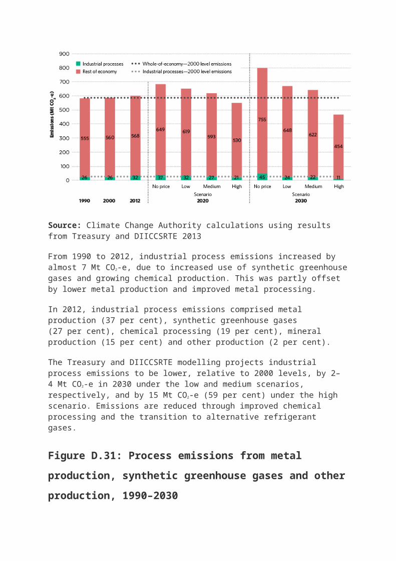
forest management—practices that increase sequestration in forests.

Combustion of fossil fuels from forestry activities, such as in logging machinery, is covered in other sectors.

Since January 2013, Australia has counted net emissions associated with forest management, cropland management, grazing land management and revegetation towards its emissions commitments under the Kyoto Protocol. LULUCF emissions presented in this section have been revised to be consistent with these new accounting rules.

LULUCF has been the biggest sectoral contributor to emissions reduction in Australia since 1990. Net emissions declined by about 85 per cent from 140 to 21 Mt CO2-e in 2012 (Figure D.36).

Figure D.36: LULUCF share of Australia’s emissions, selected

years, 1990–2030

 

Source: Climate Change Authority calculations using results from Treasury and DIICCSRTE 2013

The Treasury and DIICCSRTE modelling projects that net LULUCF emissions could decrease to 13 Mt CO2-e in 2020 and 11 Mt CO2-e in 2030 in the high scenario, or otherwise increase to 30 Mt CO2-e in 2020 and 34 Mt CO2-e in 2030 in the no price scenario (Figure D.36).

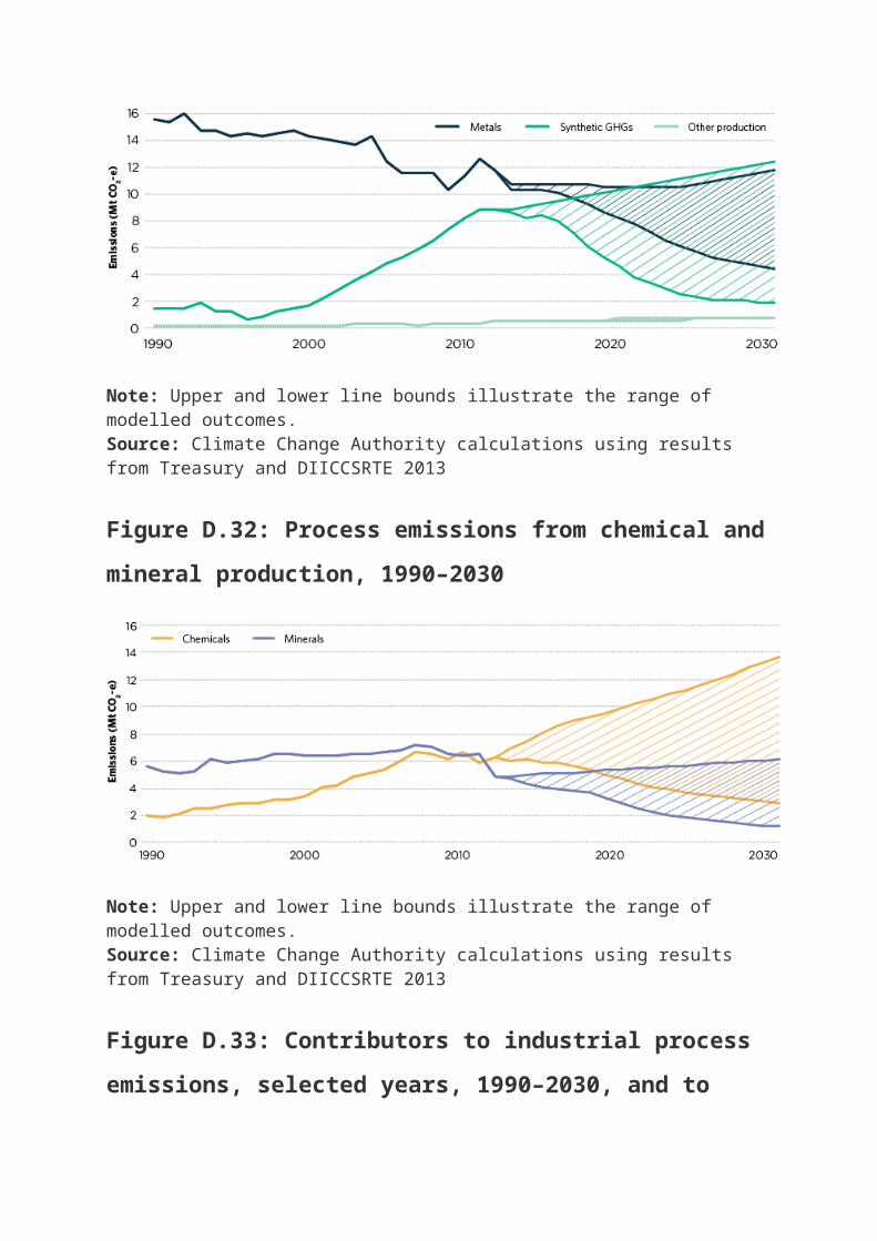
Figure D.37: Deforestation and other land use change emissions and

sequestration, 1990–2030

 

Note: Negative emissions reflect carbon sequestration. Upper and lower line bounds illustrate the range of modelled outcomes. Source: Climate Change Authority calculations using results from Treasury and DIICCSRTE 2013

D9.2 LULUCF emissions outcomes, contributors and drivers

Figure D.38 shows actual LULUCF emissions and removals by subsector from 1990 to 2030. The vast majority of LULUCF emissions and removals, both current and projected, are from forestry activities (deforestation, reforestation and afforestation, and forest management). Non-forestry activities (cropland and grazing land management and revegetation) are much smaller sources of emissions and removals.

Figure D.38: Contributors to LULUCF emissions, selected years,

1990–2030, and to change in emissions relative to 2000 levels

 

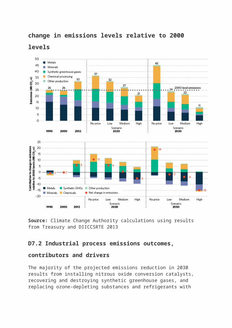
Source: Climate Change Authority calculations using results from Treasury and DIICCSRTE 2013

D9.2.1 Outcomes

The Treasury and DIICCSRTE modelling projects net LULUCF emissions may decrease by 2 Mt CO2-e to 19 Mt CO2-e from 2012 to 2030 under both the low and medium scenario, and decrease to 11 Mt CO2-e under the high scenario. Under the no price scenario, emissions are projected to increase to 34 Mt CO2-e in 2030.

Over the period from 2013 to 2020, the Treasury and DIICCSRTE modelling projects cumulative LULUCF emissions reductions associated with the Kyoto Protocol accounting changes and additional land management acitivities of 90 Mt CO2-e irrespective of price incentives. Cumulative emissions reductions are projected to rise to 126 Mt CO2-e in the medium scenario. Similarly, the ANU Centre for Climate Law and Policy estimates potential LULUCF emissions reductions of 110–115 Mt CO2-e from forest management, crop land management, grazing land

management and revegetation activities from 2013 to 2020 (Issues Paper submission, pp. 12–14).

Since 1990, deforestation emissions have declined, reflecting economic factors and also the strengthening of state and territory restrictions on land clearing regulations over the period. Between 1990 and 2011, emissions fell by over 100 Mt CO2-e to 38 Mt CO2-e, before increasing to 47 Mt CO2-e in 2012. The Treasury and DIICCSRTE modelling projects deforestation emissions will increase to 50 Mt CO2-e in 2013, remain steady to 2020, and gradually decline to 46 Mt CO2-e in 2030 under both the low and medium scenarios. Under the no price scenario, emissions are projected to increase to 52 Mt CO2-e in 2030, peaking at 54 Mt CO2-e in 2016. Recent relaxation of land clearing restrictions in New South Wales, Queensland and Western Australia may contribute to increasing emissions.

According to the Treasury and DIICCSRTE modelling, sequestration from reforestation and afforestation increased from 11 Mt CO2-e in 2000 to 25 Mt CO2-e in 2012. This was in part driven by economic conditions and forest Managed Investment Schemes, which allowed investors to deduct 100 per cent of their investment against taxable income earned elsewhere. Regulations governing these schemes were tightened in 2007 and have contributed to a reduction in tree plantation investments. ClimateWorks (2013, p. 21) reported the area of plantation forests cleared in 2012 exceeded new plantings, resulting in a reduction in the total plantation estate for the year.

The Treasury and DIICCSRTE modelling projects afforestation and reforestation sequestration will decrease to below 10 Mt CO2-e in 2020 and 2030 under all scenarios. Many of the plantations established in the early 2000s were short-term pulpwood and are nearing readiness for harvest. Due to policy uncertainty and long investment returns from tree plantations, ClimateWorks (2013, p. 31) projects a significant proportion of harvested forest land will not be returned for reforestation over the next 5 to 10 years and will instead be converted to other land use.

D9.2.2 Contributors and drivers

The main contributors to emissions and sequestration in the LULUCF sector are clearing land, planting land or forestry management (Figure D.39).

Figure D.39: LULUCF emissions and sequestration (medium

scenario), 1990–2030

 

Source: Climate Change Authority calculations using results from Treasury and DIICCSRTE 2013

Major drivers of these activities are agricultural and forestry commodity prices; input costs; and state, territory and Commonwealth land clearing regulations.

Land use decisions are influenced by relative prices of forestry and agricultural commodities. Policies, including the CFI, can affect the economic returns from these activities (see Box D.7). Historically, tax concessions for forestry have been effective in driving investment in sequestration through higher rates of afforestation and reforestation. This was witnessed in the early 2000s where Managed Investment Schemes significantly increased new tree plantations.

Commodity prices are affected by factors such as structural timber demand; demand for paper; production of paper, paperboard, plantation woodchips and pulp in developing countries; and paper recycling.

Box D.7: Emissions reduction opportunities under the CFI

Current CFI methodologies for LULUCF projects cover different types of forestry and revegetation activities, including environmental plantings, human-induced regeneration of native forests, native forest protection and reforestation.

Over 260,000 ACCUs (including Kyoto- and non-Kyoto-approved)—each worth at least one tonne CO2-e reduction—have been issued to LULUCF

projects (as at January 2014). Projected emissions reductions from the CFI between 2012 and 2030 are detailed in Appendix C of the Treasury and DIICCSRTE report (2013).

ClimateWorks (2013, p. 40) identified a range of possible CFI projects that could potentially reduce emissions by over 10 Mt CO2-e in 2020. Net Balance (2013, p. 8) suggested that including a co-benefit standard in the CFI could also broaden the market and increase the uptake of CFI projects.

D9.3 Progress in land sector emissions reduction

Currently, most land cleared in Australia is used for cattle grazing, but in the past large areas of land have also been cleared for cropping (DIICCSRTE 2013a, p. 7). Previously, the value of agricultural products has strongly influenced decisions to clear additional forested areas, with a lag of about a year between moves in agricultural prices and land clearing activities. Both farmers’ terms of trade and the amount of land clearing have decreased between the early 1970s and 2011 (DIICCSRTE 2013c, p. 8).

Land clearing, taxation and land use regulations in states and territories can influence expected returns or how easily land can be cleared or reforested. The introduction of stronger state and territory land clearing regulations in the mid 1990s reduced the rate of deforestation and emissions. This, along with economic conditions, contributed to the change in the rate of first-time clearing of undisturbed forest—which fell from 74 per cent of total land area cleared in 1990 to 35 per cent in 2011 (DIICCSRTE 2013a, p. 7).

Land clearing restrictions introduced in Queensland in 2004 and strengthened in 2009 have had the largest impact on deforestation emissions in Australia. While Queensland still has the largest deforestation emissions of any state or territory, these fell from 34 Mt CO2-e in 2007 to 19 Mt CO2-e in 2011 (DIICCSRTE 2013b, p. 29).

In 2013, both Queensland and New South Wales relaxed their land clearing restrictions, making it easier for farmers to clear trees and natural vegetation, and expand cropping operations. This is expected to put some upward pressure on emissions, although relatively stable projections for cattle numbers to 2020 suggest that this pressure will be limited in the short to medium term (Centre for International Economics 2013, pp. 21–22).

Western Australia also relaxed its land clearing restrictions during 2013. Farmers are now allowed to increase their annual land clearing rate for specified purposes from 1 to 5 hectares without a permit (Jacobs 2013).

In Tasmania, the Tasmanian Forest Agreement protects 500,000 hectares of World Heritage-listed forests from deforestation. In December 2013, the Commonwealth Government provided funding to the council overseeing this agreement for another six months. Potential changes to this agreement could increase deforestation emissions (Commonwealth 2013, p. 980).

A range of policies have been used to reduce LULUCF emissions in other countries (see Box D.8).

Box D.8: International approaches to LULUCF

Other countries have adopted regulatory and pricing approaches to preserve forests. Measures are generally designed to meet a broad range of environmental and conservation objectives, rather than solely aiming to reduce emissions.

Brazil provides an example of a regulatory approach. In the early 2000s, deforestation accounted for about 75 per cent of Brazil’s total emissions. Deforestation emissions have decreased by 82 per cent to 2011, due to stronger law enforcement, technology systems and prevailing lower agricultural prices (Climate Policy Initiative 2013, p. 7).

New Zealand provides an example of a price-based approach to LULUCF. Its Emissions Trading Scheme (ETS) was introduced in 2008 and is estimated to have reduced emissions by 77 Mt CO2-e between 2008 and 2012. This is in addition to existing forestry rules that limit the ability to harvest New Zealand native forests (New Zealand Ministry for the Environment 2013).

The Canadian province of Alberta has also adopted a price-based approach. The Alberta Offsets System, which has some similarities to the Australian CFI, provides offset credits for projects in several sectors, including LULUCF, and is used by large-emitting facilities to meet their emissions intensity reduction obligations. LULUCF activities that have approved protocols include afforestation and conservation cropping. California also includes forestry projects in its compliance offsets program under the California Cap and Trade Program, which commenced in January 2013.

D9.3.1 Other estimates of land sector emissions reductions

Grundy et al. (forthcoming 2014) reports that with strong price incentives non-harvest carbon plantations and native vegetation could greatly increase sequestration to 2050. It also reports low volumes of sequestration before 2030, even with strong price incentives, due in part to probable slow uptake of new land uses and the physical characteristics of carbon sequestration.

From 2031 to 2050, Grundy et al. (forthcoming 2014) finds average annual emission reductions of between 100 and 500 Mt CO2-e would be economically and technically feasible if payments to landholders are broadly consistent with the CFI and the carbon price trajectories in the medium and high scenarios modelled by the Treasury and DIICCSRTE (2013). The upper end of this range suggests there is potential to achieve 80–100 per cent reduction in Australia’s emissions in 2050 (compared to 2000 levels) with little or no use of international units, through a combination of land sector credits and emissions reductions in energy and other sectors.

Emission reductions from reforestation and afforestation is projected to decline in the decades after 2050 as plantings mature. Many of the LULUCF emissions reduction opportunities could create substantial co-benefits such as reduced erosion, protection of biodiversity and improved water quality.

D9.3.2 Barriers to emissions reduction

The uptake of CFI emissions reduction projects by landowners or investors depends on the amount of revenue generated and the level of risk they are willing to accept. In the case of forestry, the revenues generated will need to be sufficient to offset the opportunity cost of alternative land uses.

Specific risks and uncertainties for the CFI include:

Relative agricultural commodity prices—high terms of trade for agricultural output may work against investing in CFI projects that involve forestry on potential agricultural land. Previous estimates of reforestation potential have indicated that landowners would typically only consider reforesting non-irrigated dryland, which has relatively low agricultural returns (Burns et al. 2011, p. 24).

Price of emissions units—a volatile or uncertain market for emissions units can be a disincentive for landowners considering participating in CFI projects. Under the CFI, landowners and investors receive ACCUs for carbon sequestration projects as trees or soils sequester carbon from the atmosphere. Once the trees or soils have stored as much

carbon as they can, the project ceases to receive returns, but landowners may continue to incur management costs (Burns et al. 2011, p. 13).

Permanency—CFI projects that sequester carbon are required to maintain that sequestration ‘permanently’ (for 100 years in the case of forestry projects), which may dampen the uptake of projects. Land value can be adversely affected due to limitations on its future use (ClimateWorks 2013, p. 44).

Capital constraints—some projects will require significant upfront investment. For instance, reforestation projects generally require significant capital upfront for land preparation and planting, but will make returns over an extended time period as the forest grows.

New tree plantations have high upfront investment costs, a long project life and long payoff periods given the time taken for trees reach their peak sequestration rate. To offset some of this risk, strong financial incentives may be needed to drive investment. This is supported by Grundy et al. (2014 forthcoming), which finds that very little carbon sequestration would be supplied to 2050 at gross payments, equivalent to a carbon price, below $40/t CO2-e, with potential supply expanding with payments in the range from $40–$80/t CO2-e. Further, Polglase et al. (2011, pp. 2, 20) found that gap payments may be necessary to encourage tree plantings on marginal land where biodiversity co-benefits may be greatest.

Appendix D10 Waste

D10.1 Waste emissions overview

Waste includes solid waste and wastewater from residential, commercial and industrial activity. Waste emissions are primarily methane and nitrous oxide, which arise as organic waste decomposes in the absence of oxygen. Emissions from solid waste in landfill comprise about 80 per cent of the sector’s emissions, with wastewater accounting for about 20 per cent, and incineration and other sources for the remainder.

The waste sector is a relatively small contributor to Australia’s emissions, accounting for about 15 Mt CO2-e (3 per cent) of the national emissions total in 2012 (Figure D.40). The Treasury and DIICCSRTE modelling projects waste emissions could be about 1 per cent of total national emissions to 2030 under the medium scenario.

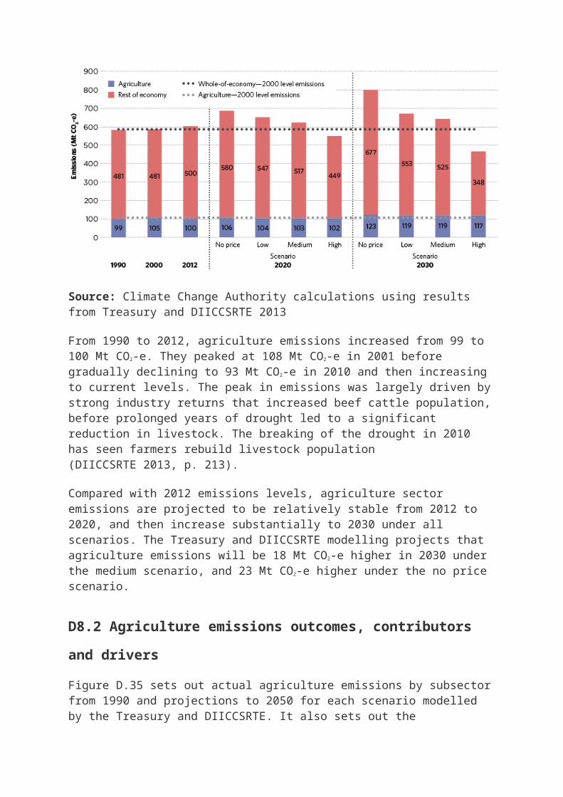
Figure D.40: Waste share of Australia’s emissions, selected years,

1990–2030

 

Source: Climate Change Authority calculations using results from Treasury and DIICCSRTE 2013

Waste sector emissions have decreased by about 8 per cent (just over 1 Mt CO2-e) since 2000, continuing the trend seen in sectoral emissions since 1990 (26 per cent decrease). This has been due to a range of policies and regulations that have diverted waste from landfill and the uptake of emissions reduction technologies, including capturing emissions for electricity generation.

Since 2000, emissions intensity of wastewater has declined by about 14 per cent and the emissions intensity of landfill by about 8 per cent (Figure D.41). In 2008, there was a large increase in the diversion of waste, resulting in a large reduction in solid waste volumes sent to landfill.

Figure D.41: Solid waste emissions intensity, 1990–2030

 

Note: Upper and lower line bounds illustrate the range of modelled outcomes. Source: Climate Change Authority calculations using results from Treasury and DIICCSRTE 2013

Figure D.42: Emissions intensity of landfill, 1990–2030

 

Source: Climate Change Authority calculations using results from Treasury and DIICCSRTE 2013

The Treasury and DIICCSRTE modelling projects total waste emissions will stabilise at about 15 Mt CO2-e by 2030 under a no price scenario, despite increases in total waste generated. Under the other modelled scenarios, emissions are projected to fall even further to between 7 and 9 Mt CO2-e (Figure D.43).

Solid waste emissions intensity is projected to fall about 30 per cent from 2000 levels to 0.47 t CO2-e per tonne of waste under the no price scenario by 2030, and to 0.18 t CO2-e per tonne under the high scenario (Figure D.41).

D10.2 Waste emissions outcomes, contributors and drivers

Since 1990, waste emissions have steadily fallen due to a range of local, state and national policies and schemes targeting the waste sector. These varied interventions have ranged from direct regulations, such as local planning laws, to market-based incentives, including the CFI, the NSW Greenhouse Gas Reduction Scheme (GGAS), the RET and the carbon pricing mechanism. These interventions have driven the diffusion of emissions-reducing technologies to landfill waste and wastewater facilities, as well as greater recycling, composting and other alternative waste treatments.

The main contributor to emissions from the waste sector is the volume of waste, which is driven by growth in population and economic activity. The main contributors to emissions reductions in the sector are the level of waste diverted for recycling or alternative waste treatments, and the extent to which the methane generated by decomposing waste is captured and destroyed. Figure D.43 shows the contribution of the two major waste streams to total waste emissions under the different modelled scenarios. Solid waste emissions comprise landfill emissions, incineration emissions and composting emissions; wastewater emissions comprise industrial, domestic and commercial wastewater.

Figure D.43: Contributors to waste emissions, selected years, 1990–

2030, and to change in emissions relative to 2000 levels

 

Source: Climate Change Authority calculations using data from Treasury and DIICCSRTE 2013

Despite continued increases in recycling and other alternative waste treatments, the Treasury and DIICCSRTE’s modelling projects the volume of waste deposited at landfills could grow by 14 per cent (3 Mt CO2-e) from 2000 levels by 2030, due to continued population and economic growth. Over the same period, in the low and high scenarios emissions can be reduced by between 58 and 70 per cent on 2000 levels. This includes a projected decline in solid waste emissions intensity of between 63 and 73 per cent on 2000 levels by 2030. Under these scenarios, emissions will fall by 4–5 Mt CO2-e from 2000 levels by 2020, and 8–9 Mt CO2-e by 2030 (Figure D.43).

Wastewater volumes are projected to grow by nearly 50 per cent on 2000 levels by 2030. Over the same period, the Treasury and DIICCSRTE modelling shows that under the same low and high scenarios, emissions can be reduced by between 10 and 20 per cent on 2000 levels. This equates to a projected decline in wastewater emissions intensity of between 40 and 46 per cent on 2000 levels by 2030. Under these scenarios, emissions will fall by 0.1–0.6 Mt CO2-e from 2000 levels by 2020, and 0.3–0.7 Mt CO2-e by 2030 (Figure D.43).

Box D.9: Waste to energy

Methane from decomposing waste can be captured from landfills or waste collection ponds and combusted to generate electricity. The electricity can be used on site or supplied to the electricity grid. Captured methane from waste is classed as biogas, a renewable source, and the emissions reductions derived from the displacement of fossil fuels are reflected in the stationary energy sector.

D10.3 Progress in waste emissions reduction

D10.3.1 Waste emissions reduction opportunities

The largest contributors to further emissions reduction in the waste sector are expected to be continued diversion of waste from landfill, methane capture and waste-to-energy. These activities are driven by a range of regulatory drivers, policy drivers and market-based incentives.

Alternative waste treatments have grown significantly since 1990, resulting in a significant amount of waste being diverted away from landfill (see Table D.7). Since this time, a major driver for the growth of alternative waste treatments has been the impact of regulatory frameworks. These have operated at all levels of government and span local planning controls, environmental safeguards and community standards, and have served to direct waste streams away from landfill where feasible.

Australian states and territories have adopted a broadly similar hierarchy of waste resource management options, in the following order:

avoiding unnecessary resource consumption as the first preference

adopting alternative waste treatments, including reuse

reprocessing, recycling and energy recovery

disposing via landfill or effluent streams.

Some states have embodied this hierarchy into legislation such as the Waste Avoidance and Resource Recovery Act 2001 (NSW).

Strategic policy frameworks have also been developed at all levels of government. The National Waste Policy, for instance, is a major national policy that was endorsed by COAG in 2009, and sets Australia’s waste management and resource recovery direction to 2020. In partnership with the states and territories, the policy establishes strategic direction and best practice in the areas of waste avoidance and waste diversion.

The management of waste continues to be a strong policy focus for state governments. For example, New South Wales recently released its Draft Waste Avoidance and Resource Recovery Strategy to 2021, for public consultation. The draft strategy includes targets for reducing waste generation, litter and landfill, and increasing recycling rates. Victoria recently released two draft waste strategies detailing how the state will invest in waste infrastructure and maximise resource recovery.

Recycling and other waste diversion activities are projected to increase under a no price scenario, contributing to the emissions reductions outlined earlier. In the future, waste avoidance and alternative waste treatments are expected to be crucial in offsetting the growing quantity of waste generated that would otherwise be sent to landfill. With appropriate policies, incentives and funding in place, Blue Environment (2011, p. 8) estimates that by 2030 as much as 70 per cent of all solid waste could be slated for resource recovery, reducing as much of 80 per cent of emissions.

Since the late 1990s, there has been a growing number of market-based schemes established in many jurisdictions across Australia to encourage the reduction of waste and emissions. The diffusion of emissions capture and waste-to-energy technologies is influenced by demand, technology costs and regulations, and also by other market-based schemes that provide price incentives, such as the RET. Since 2001 under the RET, waste facility operators have been able to earn certificates for capturing waste methane for electricity generation.

Table D.7: Total national generation of waste and disposal to

landfill, 1940–2007

Year 1940

1950 1960 1970 1980 1990 2000 2007

Waste generated (kt)

9,600

10,100

15,200

17,700

17,100

16,400

25,600

42,700

Disposed to landfill (kt)

9,600

10,100

15,200

17,700

17,100

16,400

19,600

21,300

Landfilled portion

100%

100% 100% 100% 100%

100% 77% 50%

Source: Modified from Department of the Environment, Water, Heritage and the Arts 2010

ClimateWorks (2013, p. 23) noted that between 2001 and 2011 waste operators were credited with over 6 GWh of electricity generation under the RET, representing more than 7 per cent of large-scale renewable energy generation. Waste-to-energy technologies have grown sufficiently in scale and may soon contribute about 800 GWh of electricity into the NEM annually (SKM-MMA 2012, p. 77). There is enough generation capacity from captured methane to power more than 200,000 homes, with an additional 45 MW of new landfill electricity generation projects currently in development, and a further 18 MW under assessment.

The modelling undertaken by the Treasury and DIICCSRTE includes the impact of the RET in all scenarios. Under the no price scenario, the small emissions reduction projected to 2030 can be attributed to a combination of factors, including the continuing impact of the RET.

In addition to the national RET, state-based schemes promoting effective treatment or diversion of waste have also contributed to the diffusion of emissions reduction technologies. The GGAS operated in New South Wales from 2003 to 2012 and gave operators credits to capture emissions and certificates for electricity generation from landfill gas, similar in function to the RET. This scheme helped to incentivise the uptake of landfill gas capture technologies by giving landfill operators additional revenue streams via the market for offset credits. This scheme was closed in 2012. The CFI now offers incentives for eligible landfill gas capture projects.

The CFI provides price incentives for the reduction of emissions associated with legacy waste (waste deposited prior to 1 July 2012). Since its introduction, the CFI has registered more projects related to waste than from any other sector. According to the Clean Energy Regulator (2013), the CFI has 69 registered waste projects involving gas capture, combustion and diversion in January 2014. These projects have resulted in about 3.9 million Australian carbon credit units being issued, representing a reduction in emissions of almost 4 Mt CO2-e. Given that only legacy waste is eligible for CFI credits, the CFI is projected to be most pronounced in the first few years of operation, and will decline into the future as the emissions from legacy waste decline.

The price difference between landfilling and alternative waste treatments is expected to shrink under the low, medium and high scenarios, which would make alternative waste treatment a more attractive option. There is some evidence that reducing the price difference of landfill relative to alternative waste treatments drives waste streams away from landfill (PC

2006, pp. 153–7). This has previously been addressed via increased landfill levies in some Australian states and in the UK (UK Committee on Climate Change 2013, p. 218).

D10.3.2 Barriers to waste emissions reduction

Due to a range of pricing, demand and regulatory differences across states and municipalities, the level of landfill diversionary activity differs, indicating that additional emissions reduction opportunities may exist.

The installation of new technologies involves large capital costs that may take an extended period of operation to recover. This suggests that a strong and stable price incentive or a clear and enforceable regulatory requirement would be needed to further incentivise investment in these technologies.

New waste treatment technologies and processes, such as food and electronic waste treatment and thermal treatment plants, may also face hurdles from community acceptance, land availability, local planning requirements and funding.

The level of demand can also be a barrier to effective waste diversion or emissions reduction, as towns in rural and regional areas often do not generate enough waste for operators to justify investing in costly alternative waste treatment facilities or technologies.

1 Large scale is taken to be annual sequestration of at least 0.8 Mt CO2-e for coal-fired power plants and 0.4 Mt CO2-e for gas-fired plants (GCCSI 2013c).

2 Based on a scenario that limits global emissions concentrations to 450 ppm in 2050.

3 Conversion factor applied to convert US CAFE tested mpg to New European Drive Cycle tested g CO2/km (ICCT 2012).