Embed Size (px)
Citation preview
AFIT/DS/ENP/07-01
A MULTIREFERENCE DENSITY FUNCTIONAL APPROACH TO THE
CALCULATION OF THE
EXCITED STATES OF URANIUM IONS
DISSERTATIONEric V. BeckMajor, USAF
AFIT/DS/ENP/07-01
Approved for public release; distribution unlimited

The views expressed in this dissertation are those of the author and do not reflect the official
policy or position of the Department of Defense or the United States Government.
AFIT/DS/ENP/07-01
A MULTIREFERENCE DENSITY FUNCTIONAL APPROACH TO THE
CALCULATION OF THE
EXCITED STATES OF URANIUM IONS
DISSERTATION
Presented to the Faculty of the School of Engineering Physics
of the Air Force Institute of Technology
Air University
In Partial Fulfillment of the
Requirements for the Degree of
Doctor of Philosophy
Eric V. Beck, BS, MS
Major, USAF
March, 2007
Approved for public release; distribution unlimited


Acknowledgements
Many people, my wife and family especially, are directly responsible for my successes here at
AFIT, in my career, and in my life. While the list is far too long to mention each individual
specifically, rest assured, your presence in my life was and is appreciated.
Eric V. Beck
iii
Table of Contents
Page
Acknowledgements . . . . . . . . . . . . . . . . . . . . . . . . . . . . . . . . . . . iii
List of Figures . . . . . . . . . . . . . . . . . . . . . . . . . . . . . . . . . . . . . vii
List of Tables . . . . . . . . . . . . . . . . . . . . . . . . . . . . . . . . . . . . . . ix
Abstract . . . . . . . . . . . . . . . . . . . . . . . . . . . . . . . . . . . . . . . . . xii
I. Introduction . . . . . . . . . . . . . . . . . . . . . . . . . . . . . . . . . 1
Statement of Problem . . . . . . . . . . . . . . . . . . . . . . . . . . 3
Research Objectives . . . . . . . . . . . . . . . . . . . . . . . . . . . 8
Boundary Conditions . . . . . . . . . . . . . . . . . . . . . . . . . . 9
Research Overview . . . . . . . . . . . . . . . . . . . . . . . . . . . 10
II. Uranium Ion Calculations . . . . . . . . . . . . . . . . . . . . . . . . . . 11
Relativistic Effects in Chemistry . . . . . . . . . . . . . . . . . . . . 13
Theory . . . . . . . . . . . . . . . . . . . . . . . . . . . . . . . . . . 16
The Dirac Equation . . . . . . . . . . . . . . . . . . . . . . . 17
Relativistic Effective Core Potentials . . . . . . . . . . . . . . 20
Basis Sets for Use with Shape-consistent RECPs . . . . . . . 22
Methodology . . . . . . . . . . . . . . . . . . . . . . . . . . . . . . . 22
Selection of the Reference Space . . . . . . . . . . . . . . . . 24
Results . . . . . . . . . . . . . . . . . . . . . . . . . . . . . . . . . . 25
Analysis . . . . . . . . . . . . . . . . . . . . . . . . . . . . . . . . . 30
III. The COLUMBUS-based DFT/MRCI Model . . . . . . . . . . . . . . . . . . 34
Theory . . . . . . . . . . . . . . . . . . . . . . . . . . . . . . . . . . 34
Non-relativistic Quantum Theory . . . . . . . . . . . . . . . 34
iv
Page
The Kohn-Sham Approach to DFT . . . . . . . . . . . . . . 37
Configuration Interaction and the Graphical Unitary Group
Approach . . . . . . . . . . . . . . . . . . . . . . . . . . . . . 40
Hybrid DFT/MRCI Model . . . . . . . . . . . . . . . . . . . 52
DFT/MRCI Model Implementation with COLUMBUS . . . . . . . . . 60
Density Functional Theory Interface to COLUMBUS . . . . . . 60
Correlation Energy in the Repartitioned Hamiltonian . . . . 67
CIUDG Based DFT/MRCI . . . . . . . . . . . . . . . . . . . . 68
Testing the DFT/MRCI Model Implementation within CIUDG 74
Using the COLUMBUS DFT/MRCI Model . . . . . . . . . . . . . . . . 78
Results and Analysis . . . . . . . . . . . . . . . . . . . . . . . . . . 84
Carbon Monoxide . . . . . . . . . . . . . . . . . . . . . . . . 84
Boron Fluoride . . . . . . . . . . . . . . . . . . . . . . . . . . 87
Bromine Atom . . . . . . . . . . . . . . . . . . . . . . . . . . 89
Uranium +5 Ion . . . . . . . . . . . . . . . . . . . . . . . . . 91
Uranium +4 Ion . . . . . . . . . . . . . . . . . . . . . . . . . 93
Uranyl Ion, UO2+2 . . . . . . . . . . . . . . . . . . . . . . . . 94
IV. Conclusions . . . . . . . . . . . . . . . . . . . . . . . . . . . . . . . . . . 98
Uranium Shape-Consistent RECP Accuracy Assessment . . . . . . 98
DFT/MRCI Model . . . . . . . . . . . . . . . . . . . . . . . . . . . 100
Research Objective Successes and Failures . . . . . . . . . . . . . . 108
Future Work . . . . . . . . . . . . . . . . . . . . . . . . . . . . . . . 111
DFT/MRCI with Other Correlation Density Functionals . . 111
Integration of DFT Within SCFPQ using Abelian Point Groups 112
Hybrid Exchange-Correlation Density Functional Implementa-
tion . . . . . . . . . . . . . . . . . . . . . . . . . . . . . . . . 113
Investigations into the Theoretical Basis of the DFT/MRCI
Method . . . . . . . . . . . . . . . . . . . . . . . . . . . . . . 114
Summary . . . . . . . . . . . . . . . . . . . . . . . . . . . . . . . . . 115
v
Page
Appendix A. List of Acronyms . . . . . . . . . . . . . . . . . . . . . . . . . . 118
Appendix B. DFT/MRCI Damping Parameter Selection . . . . . . . . . . . 120
Hydrogen Molecule, cc-pVDZ Basis . . . . . . . . . . . . . . . . . . 121
Hydrogen Molecule, cc-pVTZ Basis . . . . . . . . . . . . . . . . . . 123
Helium Atom, cc-pVDZ Basis . . . . . . . . . . . . . . . . . . . . . 125
Helium Atom, cc-pVTZ Basis . . . . . . . . . . . . . . . . . . . . . 127
Lithium Atom, cc-pVDZ Basis . . . . . . . . . . . . . . . . . . . . . 129
Lithium Atom, cc-pVTZ Basis . . . . . . . . . . . . . . . . . . . . . 131
Beryllium Atom, cc-pVDZ Basis . . . . . . . . . . . . . . . . . . . . 134
Beryllium Atom, cc-pVTZ Basis . . . . . . . . . . . . . . . . . . . . 136
Boron Atom, cc-pVDZ Basis . . . . . . . . . . . . . . . . . . . . . . 137
Carbon Atom, cc-pVDZ Basis . . . . . . . . . . . . . . . . . . . . . 140
Nitrogen Atom, cc-pVDZ Basis . . . . . . . . . . . . . . . . . . . . 143
Oxygen atom, cc-pVDZ Basis set . . . . . . . . . . . . . . . . . . . 146
Fluorine Atom, cc-pVDZ Basis . . . . . . . . . . . . . . . . . . . . . 149
Neon Atom, cc-pVDZ Basis . . . . . . . . . . . . . . . . . . . . . . 151
Beryllium Dimer, cc-pVDZ Basis . . . . . . . . . . . . . . . . . . . 153
Appendix C. A Procedure for Conversion of 3sd Basis Functions into Equiv-
alent 1s Functions . . . . . . . . . . . . . . . . . . . . . . . . . 156
Vita . . . . . . . . . . . . . . . . . . . . . . . . . . . . . . . . . . . . . . . . . . . 165
Bibliography . . . . . . . . . . . . . . . . . . . . . . . . . . . . . . . . . . . . . . 166
vi
List of Figures
Figure Page
1. Distinct Row Table Graph for Multi Reference Single and Double Ex-
citation Configuration Interaction Expansion (122) . . . . . . . . . . 44
2. One Body Loop Segments (124) . . . . . . . . . . . . . . . . . . . . . 50
3. Non-zero Loop Contributions to the CI Hamiltonian (120:92) . . . . . 51
4. Eigenvalue Symmetry Breaking in Two-electron Spin Coupling Example 57
5. Effect of Exponent on Eigenvalue . . . . . . . . . . . . . . . . . . . . 58
6. Density Plot of Absoulte Error Between Exact ∆E and Damped ∆E 59
7. DFT/MRCI Averaged, Absolute Error with Respect to Full Configu-
ration Interaction Results . . . . . . . . . . . . . . . . . . . . . . . . . 83
8. H2 cc-pVDZ basis DFT/MRCI Absolute Error with Respect to FCI
Results . . . . . . . . . . . . . . . . . . . . . . . . . . . . . . . . . . . 122
9. H2 cc-pVTZ basis DFT/MRCI Absolute Error with Respect to FCI
Results . . . . . . . . . . . . . . . . . . . . . . . . . . . . . . . . . . . 124
10. He Atom, cc-pVDZ basis DFT/MRCI Absolute Error with Respect to
FCI Results . . . . . . . . . . . . . . . . . . . . . . . . . . . . . . . . 126
11. He Atom, cc-pVTZ Basis DFT/MRCI Absolute Error with Respect to
FCI Results . . . . . . . . . . . . . . . . . . . . . . . . . . . . . . . . 128
12. Li Atom, cc-pVDZ Basis DFT/MRCI Absolute Error with Respect to
FCI Results . . . . . . . . . . . . . . . . . . . . . . . . . . . . . . . . 130
13. Li Atom, cc-pVTZ Basis DFT/MRCI Absolute Error with Respect to
FCI Results . . . . . . . . . . . . . . . . . . . . . . . . . . . . . . . . 133
14. Be Atom, cc-pVDZ Basis DFT/MRCI Absolute Error with Respect to
FCI Results . . . . . . . . . . . . . . . . . . . . . . . . . . . . . . . . 135
15. Be Atom, cc-pVTZ Basis DFT/MRCI Absolute Error with Respect to
FCI Results . . . . . . . . . . . . . . . . . . . . . . . . . . . . . . . . 137
16. B Atom, cc-pVDZ Basis DFT/MRCI Absolute Error with Respect to
FCI Results . . . . . . . . . . . . . . . . . . . . . . . . . . . . . . . . 139
17. C Atom, cc-pVDZ Basis DFT/MRCI Absolute Error with Respect to
FCI Results . . . . . . . . . . . . . . . . . . . . . . . . . . . . . . . . 142
vii
Figure Page
18. N Atom, cc-pVDZ Basis DFT/MRCI Absolute Error with Respect to
FCI Results . . . . . . . . . . . . . . . . . . . . . . . . . . . . . . . . 145
19. O Atom, cc-pVDZ Basis DFT/MRCI Absolute Error with Respect to
FCI Results . . . . . . . . . . . . . . . . . . . . . . . . . . . . . . . . 148
20. F Atom, cc-pVDZ Basis DFT/MRCI Absolute Error with Respect to
FCI Results . . . . . . . . . . . . . . . . . . . . . . . . . . . . . . . . 150
21. Ne Atom, cc-pVDZ Basis DFT/MRCI Absolute Error with Respect to
FCI Results . . . . . . . . . . . . . . . . . . . . . . . . . . . . . . . . 152
22. Be Dimer, cc-pVDZ Basis DFT/MRCI Absolute Error with Respect to
FCI Results . . . . . . . . . . . . . . . . . . . . . . . . . . . . . . . . 155
23. Uranium cc-pVDZ 68 Electron RECP 3sd and Converted 1s Orbitals 159
24. Uranium cc-pVDZ 68 Electron RECP 3sd and Converted 1s Orbital
Radial Probability Densities . . . . . . . . . . . . . . . . . . . . . . . 159
25. Uranium cc-pVDZ 68 Electron RECP 3sd and Converted 1s Radial
Probability Density Difference . . . . . . . . . . . . . . . . . . . . . . 160
viii

List of Tables
Table Page
1. Valence Electrons Included in Uranium PAC-RECPs . . . . . . . . . 24
2. Basis Sets for Use With Uranium PAC-RECPs . . . . . . . . . . . . . 25
3. U5+ Results, 5f1 Reference Space . . . . . . . . . . . . . . . . . . . . 26
4. U5+ Results, (5f6d)1 Reference Space . . . . . . . . . . . . . . . . . . 26
5. U4+ Results, 5f2 Reference Space . . . . . . . . . . . . . . . . . . . . 28
6. U4+ Results,(5f6d)2 Reference Space . . . . . . . . . . . . . . . . . . 29
7. U4+ Ionization Potential, 5fn References . . . . . . . . . . . . . . . . 30
8. U4+ Ionization Potential, (5f6d)n References . . . . . . . . . . . . . . 30
9. Optimized DFT/MRCI Parameters for the BHLYP Functional for Sin-
glet and Triplet States (63) . . . . . . . . . . . . . . . . . . . . . . . . 53
10. SCFPQ + Vxc and NWChem DFT Energies, CPBE96 Correlation Func-
tional . . . . . . . . . . . . . . . . . . . . . . . . . . . . . . . . . . . . 66
11. DFT/MRCI Testing Cases . . . . . . . . . . . . . . . . . . . . . . . . 76
12. Testing Results . . . . . . . . . . . . . . . . . . . . . . . . . . . . . . 77
13. Carbon Monoxide cc-pVTZ DFT/MRCI Results . . . . . . . . . . . . 86
14. BF cc-pVTZ DFT/MRCI Results . . . . . . . . . . . . . . . . . . . . 87
15. Bromine Atom cc-pVTZ DFT/MRCI Results . . . . . . . . . . . . . 90
16. U5+ DFT/MRCI Results, (5f6d)1 Reference Space . . . . . . . . . . 92
17. U4+ DFT/MRCI and MR-SOCISD Results, 5f2 Reference Space . . . 93
18. UO2+2 DFT/MRCI results . . . . . . . . . . . . . . . . . . . . . . . . 95
19. UO2+2 Calculated and Measured Fluorescent Series . . . . . . . . . . 96
20. MR-CISD Hartree-Fock Configuration Coefficients For Systems Used
for Damping Parameter Determination . . . . . . . . . . . . . . . . . 120
21. Hydrogen Molecule, cc-pVDZ Basis Set, Full CI Results . . . . . . . . 121
22. DFT/MRCI Error Analysis for Hydrogen Molecule, cc-pVDZ Basis . 121
23. Full CI Results for Hydrogen Molecule, cc-pVTZ Basis . . . . . . . . 123
24. DFT/MRCI Error Analysis for Hydrogen Molecule, cc-pVTZ Basis . 123
ix
Table Page
25. Full CI Results for Helium Atom, cc-pVDZ Basis . . . . . . . . . . . 125
26. DFT/MRCI Error Analysis for Helium Atom, cc-pVDZ Basis . . . . 126
27. Full CI Results for Helium Atom, cc-pVTZ Basis . . . . . . . . . . . 127
28. DFT/MRCI Error Analysis for Helium Atom, cc-pVTZ Basis . . . . 127
29. Full CI Results for Lithium Atom, cc-pVDZ Basis . . . . . . . . . . . 129
30. DFT/MRCI Error Analysis for Li Atom, cc-pVDZ Basis . . . . . . . 129
31. Full CI Results for Lithium Atom, cc-pVTZ Basis . . . . . . . . . . . 131
32. DFT/MRCI Error Analysis for Li Atom, cc-pVTZ Basis . . . . . . . 132
33. Full CI Results for Beryllium Atom, cc-pVTZ Basis . . . . . . . . . . 134
34. DFT/MRCI Error Analysis for Be Atom, cc-pVDZ Basis . . . . . . . 134
35. Full CI Results for Beryllium Atom, cc-pVTZ Basis . . . . . . . . . . 136
36. DFT/MRCI Error Analysis for Be Atom, cc-pVTZ Basis . . . . . . . 136
37. Full CI Results for Boron Atom, cc-pVDZ Basis . . . . . . . . . . . . 138
38. DFT/MRCI Error Analysis for Boron Atom, cc-pVDZ Basis . . . . . 138
39. Full CI results for Carbon Atom, cc-pVDZ Basis . . . . . . . . . . . . 141
40. DFT/MRCI Error Analysis for Carbon Atom, cc-pVDZ Basis . . . . 141
41. Full CI Results for Nitrogen Atom, cc-pVDZ Basis . . . . . . . . . . . 143
42. DFT/MRCI Error Analysis for Nitrogen Atom, cc-pVDZ Basis . . . . 143
43. Full CI Results for Oxygen Atom, cc-pVDZ Basis . . . . . . . . . . . 146
44. DFT/MRCI Error Analysis for Oxygen Atom, cc-pVDZ Basis . . . . 147
45. Full CI Results for Fluorine Atom, cc-pVDZ Basis . . . . . . . . . . . 149
46. DFT/MRCI Error Analysis for Fluorine Atom, cc-pVDZ Basis . . . . 149
47. Full CI Results for Neon Atom, cc-pVDZ Basis . . . . . . . . . . . . . 151
48. DFT/MRCI Error Analysis for Neon Atom, cc-pVDZ Basis . . . . . . 151
49. Full CI Results for Beryllium Dimer, cc-pVDZ Basis . . . . . . . . . . 153
50. DFT/MRCI Error Analysis for Beryllium Dimer, cc-pVDZ Basis . . . 154
51. U5+ Results From Both 3sd and 1s Converted Basis Set, 5f1 Reference
Space . . . . . . . . . . . . . . . . . . . . . . . . . . . . . . . . . . . . 161
x

Table Page
52. U5+ Results From Both 3sd and 1s Converted Basis Set, (5f6d)1 Ref-
erence Space . . . . . . . . . . . . . . . . . . . . . . . . . . . . . . . . 162
xi
AFIT/DS/ENP/07-01
Abstract
An accurate and efficient hybrid Density Functional Theory (DFT) and Multirefer-
ence Configuration Interaction (MRCI) model for computing electronic excitation energies in
atoms and molecules was developed. The utility of a hybrid method becomes apparent when
ground and excited states of large molecules, clusters of molecules, or even moderately sized
molecules containing heavy element atoms are desired. In the case of large systems of lighter
elements, the hybrid method brings to bear the numerical efficiency of the DFT method in
computing the electron-electron dynamic correlation, while including non-dynamical elec-
tronic correlation via the Configuration Interaction (CI) calculation. Substantial reductions
in the size of the CI expansion necessary to obtain accurate spectroscopic results are possible
in the hybrid method. Where heavy element compounds are of interest, fully relativistic
calculations based upon the Dirac Hamiltonian rapidly become computationally prohibitive,
as the basis set requirements in four-component calculations increase by a factor of two or
more in order to satisfy kinetic balance between the large electronic components and small
positronic components, while the size of the MRCI Hamiltonian quadruples with respect to
a non-relativistic calculation. In this hybrid method, applications to heavy element com-
pounds such as bromine and uranium were accomplished through the use of relativistic
effective core potentials, allowing for the first time both scalar relativistic and spin-orbit
effect treatment necessary for the accurate calculation of electronic excitation energies in
heavy elements in a Density Functional Theory Multireference Configuration Interaction
Hybrid Model (DFT/MRCI) method. This implementation of the original hybrid method,
developed by Grimme and Waletzke, was modified to remove inherent spin-multiplicity lim-
itations, as well as reduce the number of free parameters used in the method from five to
three.
The DFT portion of the hybrid method used 100% Hartree-Fock (HF) exchange and
an electron correlation-only density functional as the basis for a modified Graphical Unitary
Group Approach (GUGA) based CI calculation. The CI algorithm was modified to expo-
nentially scale the off-diagonal matrix elements of the CI Hamiltonian in order to reduce the
double counting of electronic correlation computed by both the DFT correlation functional
xii
and the CI calculation. The scaling applied to the interaction between states in the CI
calculation exponentially decreased to zero as the energy difference between states grew.
This algorithm left interactions between degenerate or nearly degenerate states unscaled,
while rapidly scaling to zero interactions between states widely separated in energy.
The two empirical parameters which controlled this off-diagonal matrix element scaling
were determined through the use of a training set of light atoms and molecules consisting
of H2, He, Li, Be, B, C, N, O, F, Ne, and Be2. The average DFT/MRCI errors with respect
to exact Full Configuration Interaction (FCI) results on this training set was 9.0559 milli
Hartrees (mH) over 11 atomic and molecular systems. CI expansion length tailoring through
virtual orbital freezing. Consistently favorable results were obtained when virtual orbitals
30-40 Electron Volt (eV) above the highest occupied molecular orbital were frozen, providing
the best trade off between method accuracy and reduction in CI expansion length. Using
this approach to paring the CI expansion length, reductions in the size of the CI expansions
of a factor of 25-64 were achieved.
The values of the two off-diagonal scaling parameters were determined by minimiz-
ing the average absolute error between the DFT/MRCI and exact FCI calculations for
all test atoms and molecules combined. The values of the parameters obtained for the
100% HF exchange and Perdew Burke and Ernzerhof (PBE) 1996 Generalized Gradient
Approximation (GGA) correlation functional combination were p1=0.96 and p2=2.5.
After the scaling parameters were determined using the training suite of atoms and
molecules, the method was applied to carbon monoxide, boron fluoride, the bromine atom,
the uranium 5+ and 4+ ions, and the uranyl (UO2+2 ) ion. In all cases, the correct ordering of
ground and excited states was obtained using the DFT/MRCI model. In CO, a reduction in
overall error of 26% with respect to Time Dependent Density Functional Theory (TDDFT)
was observed over 6 ground and excited states. A reduction in overall error of 42% with
respect to TDDFT was observed in 5 ground and excited states of BF, while an accuracy
with respect to experiment of 11-22% for electronic excitation energies for the first excited
states of the bromine atom and uranium 5+ and 4+ ions was observed. Final application
of the model to the uranyl ion compared favorably with observed uranyl fluorescent series
xiii

in crystals, and was obtained with an order of magnitude reduction in the computational
effort with respect to a traditional, wave function based quantum chemistry approach.
xiv
A MULTIREFERENCE DENSITY FUNCTIONAL APPROACH TO THE
CALCULATION OF THE
EXCITED STATES OF URANIUM IONS
I. Introduction
Actinide chemistry, in particular, the chemistry of uranium, continues to be of in-
tense interest in many applications. Design, performance, aging, and disposal of nuclear
fuel components, the environmental transport of uranium compounds lingering in mines
and ore processing waste, as well as material delivered through depleted uranium muni-
tions all require a thorough understanding of the chemistry of uranium. Furthermore, the
nuclear weapon stockpile stewardship program1 demands a thorough understanding of the
processes by which uranium components age, as well as the effect aging has on the reli-
ability and performance of nuclear weapons. A cornerstone of the stockpile stewardship
program is theoretical modeling and simulation of the basic physics and chemistry involved
in the design, manufacture, maintenance, and operation of a nuclear weapon. Non-invasive
electronic spectroscopic methods may be used to diagnose the extent of nuclear weapon
component aging (66).
Of particular importance in the underlying chemistry of these uranium compounds is
the oxidation state of the uranium atom. Uranium, like most early actinides, can possess a
wide range of oxidation states, ranging from +3 to +6, due in part to chemical activation
of the uranium 5f orbitals via relativistic effects which will be described shortly. The
oxidation state of uranium can be influenced by its local chemical environment, which in
turn influences the geometry of the uranium oxide compounds. The uranium oxidation state
can be inferred through spectroscopic measurements studies, which are useful in nuclear
forensics and environmental monitoring.
Structural studies performed using x-ray or neutron diffraction on uranates concur
that uranium oxides tend to occur in either an elongated or flattened octahedral geometry
1http://www.nnsa.doe.gov/
1
in uranium compounds . The consensus of these studies show that uranyl-like configurations
dominate, where the tightly bound, linear UO2+2 ion is present, surrounded by three to
five equatorial ligands, with axial uranium-oxygen bonds lengths ranging from 1.7-2.0 A.
Equatorial bond lengths cluster in the range of 2.0-2.4 A, depending on the ligand species
(40) (49) (27) (38) (128) (134) (116) (141). Particularly thorough reviews of the structure
of uranium oxide are given in papers by Burns et al (26) (27), Miller (89), and by Katz (75)
as well as in the Gmelin Handbook (29) and Rabinowitch (111). Rare distorted tetrahedral
configurations or uranium oxides have been reported, with uranium-oxygen bond lengths
on the order of 1.9 A(69).
X-ray photoelectron spectroscopy, a particular method of high energy electronic spec-
troscopy, provides insight into the electronic structure of these uranium oxides, however,
the resolution to probe, in detail, the electronic structure of the valence region below 5 eV
makes such methods insensitive to uranium bonding. Despite this lack of sensitivity, x-ray
photoelectron studies have proven useful in probing the electronic structure of inner valence
and core-like electrons in uranium oxide compounds (60) (132) (44) (133). Electronic tran-
sition energies to and from the uranium 5d, 6p, and 6s levels are typically probed in these
studies, yielding insight into the nature of these higher energy transitions.
Most insight into lower energy valence transitions in uranium oxides, where photolu-
minescence originates, has been gained from electronic photoluminescence measurements of
uranium doped crystal studies. It is in the valence region where x-ray studies lack the sen-
sitivity or resolution to fully characterize the electronic structure of the bonding. In these
crystal studies, a distorted octahedral coordination with a tightly bound, central, linear
uranyl ion is typically found (84) (129) (130) (5) (22) (18) (19) (93) (80). Photolumines-
cence in these compounds, attributed to ligand to metal charge transfer transitions from
uranium in a +6 oxidation state to oxygen ligands results in a yellow-green fluorescence
peaking at 18,000 to 21,000 cm−1. Crystal field and ligand effects lead to relatively modest
perturbations to this fluorescence spectra, typically on the order of 1000 cm−1. Lifetimes
vary, but are typically of the order of microseconds. Excellent overviews are contained in
(61) (29) and (111). One of the most detailed analyses of the electronic and vibrational
spectra of the uranyl ion was performed by Denning based on a series of experimental work
performed in the 1970s (43) (45) (42). In his study, Denning verified earlier analysis (111)
2
that the linear uranyl ion is particularly stable, with bond dissociation energies for the
uranyl ion of 700 kilo Joule (kJ) per mole. He also finds that the uranyl ion is chemically
inert. Isotopic oxygen exchange in uranyl has a lifetime of over 40,000 hours. Denning’s
examination of uranyl spectra in CsUO2Cl4 show that the 5f electron shell lies below the 6d,
with f and d separation increasing as with increasing uranium oxidation state. The uranium
5f shell is responsible for most of the ligand interactions, and the nature of the character-
istic green-yellow luminescence in uranium compounds appears to be from the presence of
low-lying, non-bonding orbitals in the 5f shell. Denning’s examination of the polarized, low
temperature crystal spectroscopy shows that the luminescence origins can be attributed to
the first two bands in the absorption spectra, and that the the low-lying excited states have
even parity. Transitions from these even-parity excited states to the even-parity ground
state are parity forbidden, and thus are magnetic dipole or electric quadrapole transitions
(41). A few studies (99) (94) report a red luminescence which is attributed to fluores-
cence originating from a distorted tetrahedral coordination of uranium with energies in the
neighborhood of 15,000 cm−1.
More recently, laser spectroscopic techniques have been applied to the analysis of
uranium oxides. Time resolved laser induced fluorescence characterization of uranium con-
tamination at Hanford was performed by Wang et al (136). Additionally, laser spectroscopy
studies on uranium in frozen matrices have been performed by Lue (83) and (3).
Statement of Problem
While there is a large amount of experimental data on the various thermo chemical
properties of uranium (75) (137), theoretical modeling of the spectra of this element has
progressed more slowly. Ab initio quantum mechanical theoretical techniques have made
great strides in understanding molecules consisting of lighter elements, and computational
methods have been quite successful in predicting thermodynamic and spectroscopic prop-
erties of these compounds. There are two main reasons for this disproportionate difficulty
in predicting the electronic spectra for heavy element compounds.
The first difficulty is that relativistic effects for actinides are significant enough that
perturbation treatments are inadequate, thus requiring a method that incorporates these
effects throughout the calculation. This is in stark contrast to lighter molecules where rela-
3
tivistic effects can be neglected in all but high-precision theoretical calculations (108:3787-
3788) (7:1-27).
There are three main relativistic effects in atomic and molecular chemistry, each
roughly the same magnitude, all of which scale approximately as Z4, where Z is the nuclear
charge (108). The first main relativistic effect is considered a direct effect, consisting of a
radial contraction of atomic orbitals, along with a stabilization of the energy level of the
electronic state. This effect is due primarily to the relativistic mass increase as electron
velocities near the nucleus become appreciable fractions of the speed of light. Electron or-
bitals having high densities near the nucleus, where electron speeds are largest, experience
the largest contraction. For example, in uranium this relativistic contraction is roughly 26%
when compared with the non-relativistic Bohr radius. All atomic orbitals have some den-
sity near the nucleus, therefore, all atomic orbitals experience some contraction. However,
the inner s- and p- orbitals nearest the nucleus experience the most contraction (108). In
light-element molecules, this orbital contraction is small and negligible in all but the highest
precision calculations, but the effect becomes large in actinide elements such as uranium.
The second relativistic effect is an indirect effect, and it consists of a radial expansion and
destabilization in the electronic energy levels of outer atomic orbitals. This is due to in-
creased effective nuclear charge screening by the inner, contracted orbitals, reducing the
effective nuclear charge experienced by the outer electrons. Additionally, relativistic con-
traction of the inner s- and p- electron shells increase the electron density near the nucleus,
crowding out the outer d- and f - electron shells. This is due to the fact that there is a
decrease in electron density near the nucleus for orbitals with increasing orbital angular
momentum. Thus, the direct orbital contraction competes with the indirect orbital expan-
sion. The orbital expansions and contractions can affect bond lengths and force constants
(108), which in turn affect molecular vibrational frequencies. The final relativistic effect
that falls naturally out of the Dirac Lorentz covariant theory for the electron, described in
more detail in chapter two, is spin-orbit splitting of states. Spin-orbit splitting of states is
responsible for the most pronounced deviations of heavy elements in the period table from
lighter elements in the same column. The yellowish color of gold, while silver is colorless is
one striking example. Silver, a lighter element with less pronounced relativistic effects, has
an absorption spectra in the ultraviolet, while gold, a heavier element, has an absorption
4
spectra in the visible spectrum, a direct result of a combination of all three relativistic ef-
fects. The inert pair effect observed in the ionization potential of lead versus tin is another
example of spin-orbit splitting producing chemically relevant effects. In lead the relativistic
effects stabilize and split the 6p electron shell into a 6p 1
2
and a 6p 3
2
shell, resulting in a full
and relatively inert 6p 1
2
shell. The effect is much less pronounced in tin, resulting in a much
lower ionization potential.
For lighter elements, relativistic effects are typically done through perturbative cor-
rections based on the Dirac covariant theory of the electron to the non-relativistic solutions
to the Schrodinger equation, because the magnitude of the relativistic effects for elements
in the first two rows are small. For these lighter elements, the electron-electron interactions
are much larger than the relativistic corrections, which accounts for the success of pertur-
bative approaches. Unfortunately, such perturbative methods fail on heavy elements such
as uranium, as the relativistic effects can be of the same magnitude as the electron-electron
interaction. Successfully incorporating relativistic effects in heavy element calculations are
all based on solving the fully-relativistic, many electron Dirac equation. Because the Dirac
theory results in a coupling between the electron and positron, each with two spin com-
ponents, the wave function involved is four dimensional for a one-electron system, and 4N
dimensional for a N electron system. State-of-the-art calculations using the full Dirac model
involve single heavy atoms, or very small molecules, and at present are incapable of com-
puting excited states of these systems, because such calculations require multi reference
methods which rapidly become computationally prohibitive within a four-component fully
relativistic framework. One additional complication in using a fully-relativistic Dirac model
for computational chemistry is that there must be kinetic balance between the electronic
and positronic basis sets. The reason for this is that the electronic and positronic compo-
nents in the Dirac four-component model are not independent, but they are related by the
expression
ψSC =~σ · ~pE +m
ψLC , (1)
where ψSC and ψLC are the small and large component wave functions, respectively, ~σ is a
Pauli spin-matrix, ~p is the momentum, E is the total energy and m is the electron rest mass.
The speed of light in Equation 1 is set to unity. The result of this kinetic-balance requirement
5
is that for every basis electronic basis function used, there needs to be at least two positronic
basis functions, one with angular momentum quantum number L+ 1 and one with angular
momentum quantum number L − 1. Thus, a four-component, fully relativistic calculation
uses a basis set three times larger than a corresponding, non-relativistic calculation.
A second computational difficulty is the sheer number of electrons to deal with in
actinide compounds. Common uranium oxide compounds such as UO2 have 108 electrons,
while more complex oxides such as U3O8 has 340 electrons. The most common approach
for calculating excited states of atoms and molecules is CI, which will be discussed in more
detail in chapter three. Briefly, CI is a computational method where the electronic wave
function is expanded in terms of an orbital basis that includes both ground and excited state
electronic configurations. By including all possible combinations of electron occupation in
the orbital expansion basis, a FCI calculation is achieved, which is an exact solution to
the non-relativistic Schrodinger wave equation within the approximation of the finite basis
set. Despite this fact, CI has some serious limitations, namely, that CI calculations quickly
scale to computational impracticality on modern computers. For a calculation with K basis
functions and N electrons, the FCI calculation scales roughly as (2KN )N (127). Taking the
U3O8 example with N = 340 and a modest, cc-pVDZ basis set with two contracted basis
functions per shell results in 196 electronic basis functions. Kinetic balance requirements add
an additional 392 positronic basis functions, for a total of K = 588 basis functions. Thus, in
the fully-relativistic, four-component FCI calculation, there are roughly (1176340 )340 possible
N -electron configurations. Even a non-relativistic treatment, with only 196 electronic basis
functions is impractical, with (392340 )340 or 1021 possible configurations in a FCI Hamiltonian.
Accurately treating such large numbers of electrons with an all-electron FCI method is
computationally prohibitive today. Truncating the CI calculation to a lower excitation
level, say single and double excitations only, is a more tractable computational problem.
Truncated Configuration Interaction Singles and Doubles (CISD) scales roughly as (2K)2N2
(127). Even then, in the case of the four-component calculation, the truncated CI yields
a Hamiltonian with dimension over 1011, still too large for modern computers. The non-
relativistic, truncated calculation is smaller yet, with a Hamiltonian with dimension of the
order of 1010 configurations, barely within reach of modern computers and algorithms. These
examples illustrate the computational problem one encounters with all-electron methods,
6

and the additional complexity added by accounting for relativistic effects. A popular way
around these problems is through the use of Relativistic Effective Core Potentials (RECPs).
The Relativistic Effective Core Potential (RECP) approach is a compromise between
the full Dirac description, and the non-relativistic model. RECPs are covered in greater
detail in chapter two. Briefly, the RECP approach begins with atomic calculations using
the full Dirac equation. An artificial separation between core electrons and valence elec-
trons is selected, frequently based on hypotheses on which valence shell electrons are most
important in chemical bonding. Those electrons selected to be in the core are replaced in
the Hamiltonian by a potential energy term, leaving only the valence electrons to be explic-
itly modeled. This approach incorporates relativistic effects from a Dirac description of the
atom directly into the core electrons, and has the added utility in reducing the large number
of electrons present in heavy elements. These relativistic effective core potentials are then
used in non-relativistic calculations, which can be used to compute excited states of atoms
and molecules. Because the core electrons experience the most pronounced relativistic ef-
fects, calculations performed using these core potentials can produce results within a few
percent of experimental measurements of electronic spectra. Armed with these relativistic
effective core potentials, one can incorporate relativistic effects accurately and efficiently
into non-relativistic calculations. With this freedom, one can then search for the most effi-
cient non-relativistic algorithms available for calculating ground and excited states of atoms
and molecules.
DFT is another successful alternative alternative to CI. DFT is a computational
algorithm for solving the time independent, the Schrodinger wave equation, (35:245) (106:26-
29) (127:40)
Hψ (~x1, ~x2, . . . , ~xn) = Eψ (~x1, ~x2, . . . , ~xn) , (2)
with E being the energy. A more thorough discussion of DFT is undertaken in chapter three,
only a brief overview is given here. Unlike more traditional methods for solving equation
2, DFT is not based on N -dimensional abstract wave functions in Hilbert space, but on
the physically realizable, 3-dimensional electron density. The success of DFT is based
on the accuracy inherent in the electron density functional responsible for the electron-
electron exchange and correlation energies. While DFT is exact, in principle, for the ground
7
state, current research has produced approximations for this exact exchange-correlation
density functional. An additional attractive feature of DFT is the fact that it can produce
remarkably accurate results for ground state geometries and vibrational frequencies very
efficiently. DFT algorithms scale computationally on the order of(
K4)
at a maximum, with
some methods approaching linear scaling in the number of basis functions. Unfortunately,
no method is known by which a DFT calculation, using a particular density functional
approximation, can be systematically improved by improvements in the basis set or through
perturbative corrections to the effective Hamiltonian. Extensions of DFT to solve the time-
dependent Schrodinger equation exist, known as TDDFT, but the accuracy of TDDFT is
poor when applied to calculated excited states of atomic and molecular systems where open-
electron shells with large degeneracies can produce a range of spin-multiplicity states that are
close in energy. Despite these drawbacks, DFT remains a computationally efficient way to
compute electronic-electron correlation in atoms and molecules with excellent computational
scaling, unlike the FCI or truncated CI.
Grimme (62) and Grimme and Waletzke (63) proposed a model which addressed the
accuracy of DFT in open-shell and degenerate cases as well as calculating excited states.
Their model combined a DFT calculation to the CI computational framework, resulting in a
hybrid method which is designed to address the deficiencies of DFT with nearly degenerate
states of multiple spin-multiplicities that are close in energy. By forming a hybrid DFT
and CI method for computing excitation energies, Grimme and Waletzke found they could
dramatically reduce the size of the CI expansion necessary to achieve results that were
more accurate than TDDFT results. Their method demonstrated accurate calculations on
excited states in their hybrid model with reductions in the CI expansion sizes on the order
of a factor of hundreds to thousands.
Research Objectives
The goal of this research is to design, implement, and test a hybrid DFT/MRCI algo-
rithm within the COLUMBUS relativistic quantum chemistry program suite. Final validation
of the research goal will be through application of the DFT/MRCI model to the uranium
+5 and +4 ions, as well as the uranyl (UO2+2 ) ion. The U5+ ion will demonstrate the
ability of this modeling implementation to effectively compute the excitation energy of an
8
odd-electron heavy element with both scalar relativistic and spin-orbit coupling of non-
singlet and triplet spin multiplicities. The U4+ ion calculation will demonstrate the same
capability, but on an even-electron heavy element, with spin-orbit coupling between singlet,
triplet and higher multiplicities. These DFT/MRCI calculations will be assessed against
equivalent Multi-reference Spin-Orbit Configuration Interaction Singles and Doubles (MR-
SOCISD) calculations and experimental measurements of the excitation energies. Calcu-
lations of the uranyl ion will demonstrate this implementation of the DFT/MRCI model
for a even-electron molecule containing a heavy element, with spin-orbit coupling between
singlet, triplet, and higher multiplicities. The uranyl DFT/MRCI calculations will be com-
pared with equivalent MR-SOCISD calculations and various crystallographic measurements
of uranyl fluorescent series. In addition to spin-orbit effects, all heavy element calculations,
including uranium, will model scalar relativistic effects as well, a capability absent in the
most recent work by Kleinschmidt et al (77).
Boundary Conditions
In order to determine two free parameters crucial to the hybrid DFT/MRCI method,
focus was placed on small, light atoms with modest basis sets, where full configuration
interaction results were obtainable. This limited the damping parameter training set to the
first two rows of the period table, with relatively small double- and triple-ζ quality basis
sets.
To assess of the performance of the model following determination of the damping
parameters, several well studied systems were chosen. The carbon monoxide molecule was
selected from the published results of Grimme and Waletzke to validate the new code by
comparison with their implementation results. The boron fluoride molecule was chosen to
reproduce published spin-orbit coupling results obtained by Kleinschmidt et al (76). The
boron fluoride molecule has a small spin-orbit splitting on the order of 20 cm−1. The
bromine atom, which exhibits a spin-orbit splitting of the ground state on the order of 3600
cm−1, was chosen to assess the performance of this model on a heavy, odd-electron doublet
atom with relatively large relativistic effects.
9
The uranium +5 and +4 ions were chosen since MR-SOCISD results as well as mea-
sured experimental excitation energies were available for comparison. The uranyl ion was
also chosen because of it’s importance in uranium chemistry, and it’s electronic spectra has
been thoroughly studied, both experimentally and theoretically.
Research Overview
Chapter two describes the underlying theory, methodology and results of traditional ab
initio Multi-reference Configuration Interaction, Single and Double Excitations (MR-CISD)
calculations on the excited states of the U5+ and U4+ ions. The excited states of these ions
are calculated and assessed versus measured experimental excitation energies using a cc-
pVDZ quality basis set and a series of shape-consistent RECP with spin-orbit potentials.
Accuracy of the 60 electron, 68 electron, and 78 electron RECPs was compared to measured
experimental values in order to determine the most effective core-valence choice when using
shape-consistent core potentials in uranium calculations.
Chapter three describes the theory underlying the hybrid DFT/MRCI method, as
well as the implementation of the model within the COLUMBUS quantum chemistry program
suite. The results of the testing and validation of the model implementation are described,
as are the results from calculations using the COLUMBUS-based DFT/MRCI hybrid model to
carbon monoxide, boron fluoride, bromine, uranium +5 an +4 ions, and the uranyl ion.
Finally, an overall discussion of conclusions, both for the MR-SOCISD results on the
U4+ and U5+ ions, as well as the performance of the DFT/MRCI model as implemented
in this research is in chapter four. Success in achieving the research objectives will be
examined, and final suggestions for future research will be made.
10
II. Uranium Ion Calculations
Assessment of the accuracy of calculations involving actinide elements is difficult, because of
a sparsity of well-characterized, gas-phase experimental measurements. Part of the problem
lies in the fact that interpretation of measured spectra can be complicated by the fact that
many actinide compounds can be difficult to prepare in the gas-phase. Interpretation of
condensed phase measurements can be complicated by crystal field effects or by the purity
of the samples involved.
For example, the uranyl ion, UO2+2 , has received intense theoretical scrutiny, and
it is often used to benchmark theoretical methods involving uranium. A large, but hardly
exhaustive list of recent calculations are contained in the references (34) (32) (105) (33) (85)
(39) (64) (57) (74) (72) (142). The chemical stability of the uranyl ion, and its presence in
a majority of uranium compounds found in nature, as well as the relative insensitivity of
its electronic spectra to its chemical environment make it an excellent candidate for these
benchmarking studies. However, the lack of precise gas-phase measurements of the spectra of
the uranyl ion limits its usefulness in assessing the accuracy of calculated electronic spectra.
Variations on the order of 1000 cm−1 in the uranyl ion fluorescent spectra occur due to ligand
influences (111), limiting the precision of comparisons with theoretical models. Attempts
have been made to calculate the electronic spectra of uranyl in crystalline environments (86)
(105) (8).
One solution is to perform calculations using atomic systems, for which gas-phase
measurements have been performed and the resulting spectroscopic states are well char-
acterized. For uranium, numerous experimental measurements of the electronic spectra of
the neutral atom (90) (91) (36), as well as charged ions (17) (46) (100) (117) (139) (13)
(23) exist in the literature. All these gas-phase studies of the neutral uranium atom and
the +2, +3, +4 and +5 ionic species indicate that the low lying electronic transitions are
predominately due to 5f to 5f electronic excitations, which are parity forbidden. These
selection rule forbidden transitions result in faint yet sharp line spectra that are relatively
unaffected when examined in uranium doped crystals or aqueous solutions, indicating that
the 5f orbitals in uranium are not dominant in ligand bonding. A search through the lit-
erature reveals surprisingly few computational studies of atomic uranium species. A brief
summary of more recent calculations include predictions of the second through fourth ion-
11
ization potential of neutral uranium was performed by Cao and Dolg (28), a Dirac-Hartree
Fock investigation of dipole radiative parameters for uranium VI (15) by Biemont et al, and
an investigation by Barandiaran et al of the bond lengths of fn and fn−1d1 states of U4+ as
defects in chloride hosts (8) using Complete Active Space Self Consistent Field (CASSCF)
with a spinfree relativistic Ab Initio Model Potential Hamiltonian. Barandiaran et al found
that the 5f electrons are shielded by the 6p electrons, which determine the bond lengths
in fn configurations, while in fn−1d1 configurations, an f electron penetrates the shield-
ing effects of the 6p electrons and interacts with the ligands, causing a shortening of bond
lengths in general. Seojou and Barandiaran investigated the structure and spectroscopy of
U3+ defects in Cs2NaYCl6 (118), and their findings supported the conclusions reached by
Denning et al, in that 5f to 6d transitions are responsible for the photoluminescence in the
14,000 to 21,000 cm−1 range. Fedorov et al performed an in-depth ab initio study of the ex-
cited states of uranium (55) using a transformed two-component Douglas-Kroll all electron
method and spin-orbit multi configuration perturbation theory. Using this method, they
calculated 48 odd-parity states of neutral uranium to within 1000-2000 cm−1 accuracy with
respect to experiment. An older Dirac-Hartree Fock calculation by Eliav et al (53) used a
coupled cluster method in order to predict ionization potentials and excitation energies in
the uranium +4 ion. The excited states they computed using this four-component method
with single and double coupled cluster excitations predicted the ordering of the U4+ states
correctly with a reported average error in the excitation energies of 114 cm−1.
Using the experimental measurements, as well as the theoretical results found in the
calculations described above, an accurate assessment of the theoretical method can be per-
formed and be used to guide the choice of ab initio methods, and active spaces. In addition,
understanding the uranium ion atomic systems can yield greater insight into the molecu-
lar structure of uranium compounds, since the low-lying excited states are dominated by
f → f electronic transitions which are fairly insensitive to ligand influences. One of the
major challenges to accurate quantum chemical calculations on heavy element atoms is a
result of the importance of relativity in the electronic structure of high-Z elements.
12
Relativistic Effects in Chemistry
Relativistic effects in chemistry have been studied since the 1970s, with pioneering
work by Pitzer (107), Pyykko and Desclaux (109). Many reviews of relativistic effects in
chemistry can be found in the literature (109) (107) (108) (101) (73) (6) .
There are three main relativistic effects in atomic and molecular chemistry, all of which
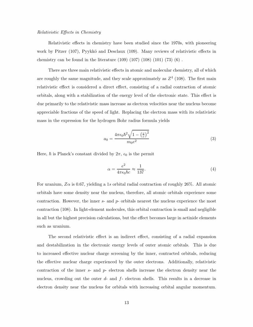
are roughly the same magnitude, and they scale approximately as Z4 (108). The first main
relativistic effect is considered a direct effect, consisting of a radial contraction of atomic
orbitals, along with a stabilization of the energy level of the electronic state. This effect is
due primarily to the relativistic mass increase as electron velocities near the nucleus become
appreciable fractions of the speed of light. Replacing the electron mass with its relativistic
mass in the expression for the hydrogen Bohr radius formula yields
a0 =4πε0~
2√
1 −(
vc
)2
m0e2(3)
Here, ~ is Planck’s constant divided by 2π, ε0 is the permit
α =e2
4πε0~c≈ 1
137. (4)
For uranium, Zα is 0.67, yielding a 1s orbital radial contraction of roughly 26%. All atomic
orbitals have some density near the nucleus, therefore, all atomic orbitals experience some
contraction. However, the inner s- and p- orbitals nearest the nucleus experience the most
contraction (108). In light-element molecules, this orbital contraction is small and negligible
in all but the highest precision calculations, but the effect becomes large in actinide elements
such as uranium.
The second relativistic effect is an indirect effect, consisting of a radial expansion
and destabilization in the electronic energy levels of outer atomic orbitals. This is due
to increased effective nuclear charge screening by the inner, contracted orbitals, reducing
the effective nuclear charge experienced by the outer electrons. Additionally, relativistic
contraction of the inner s- and p- electron shells increase the electron density near the
nucleus, crowding out the outer d- and f - electron shells. This results in a decrease in
electron density near the nucleus for orbitals with increasing orbital angular momentum.
13
The direct orbital contraction competes with the indirect orbital expansion, which can
affect bond lengths and force constants (108). These effects are observed in the spectra
of heavy-element molecules. Spin-orbit coupling is another important spectroscopic effect
which arises naturally from a Lorentz covariant description of the electron.
Intrinsic electron spin is a natural result of a Lorentz-covariant description of the
quantum mechanical wave equation (7:76-78,116). This spin angular momentum couples
with the electron orbital angular momentum, lifting degeneracy in atomic orbitals with
angular momentum. Of the three effects, spin-orbit coupling has the largest impact in
atomic and molecular spectra, even for low-Z atoms and molecules. For light atoms, a
perturbative treatment of spin-orbit coupling known as Russell-Sanders coupling, or L-S
coupling, often yields sufficient accuracy for electronic transition energies. This coupling
scheme treats magnetic spin-orbit coupling as a small perturbation to the electron-electron
electrostatic interaction. Orbital angular momentum and spin angular momentum are still
approximately constant quantum numbers in this coupling scheme, where the total orbital
angular momentum , L, total spin angular momentum, S, and total angular momentum, J
commute with the many-electron Hamiltonian in Russell-Sanders coupling scheme. Atomic
states are described by term symbols 2S+1LJ . Traditional spectroscopic notation is used
for the total orbital angular momentum, with S representing zero total orbital angular
momentum, P representing one unit of orbital angular momentum and so on. J is the total
angular momentum of the electron, given by the sum of orbital and spin angular momenta
(58:69-74) (140).
On the other end of the perturbation spectrum, more appropriate for very heavy
atoms, the electron-electron electrostatic interaction is treated as a perturbation to the mag-
netic spin-orbit coupling. This coupling scheme is known as j-j coupling. In this coupling
scheme, neither L nor S commute with the Hamiltonian. However, the total angular mo-
mentum, J , still commutes with the atomic Hamiltonian (58:74-76) (140). Most elements
on the periodic table fall between these two perturbation extremes, and so intermediate
coupling is more appropriate than either perturbative treatment. Intermediate coupling is
not a separate coupling scheme, but occurs as deviations from the separate perturbative
treatments given by L-S and j-j coupling (58:77) (140).
14
Electron spin additionally has an important affect on the symmetry of molecules.
Under the assumption that the total electronic wave function can separated into the product
of a spatial and spin wave functions, each wave function may possess separate symmetry,
and the total, observable state symmetry is given by the direct product of the spatial and
spin symmetries. For example, singlet spin states are completely symmetric, while triplet
spin states transform like the components of the angular momentum operator. A completely
symmetric spatial wave function multiplied by a triplet spin wave function will not be totally
symmetric. For systems with a spin-orbit Hamiltonian, the symmetry point groups can have
twice the number of symmetry operations, and are called double point groups. This doubling
of the order of the symmetry point groups is due to the introduction of half-integral angular
momentum values. Systems possessing an even number of electrons obey Bose-Einstein
statistics, and the total wave function of these bosonic systems is symmetric with respect to
rotations by 2π. Systems possessing an odd number of electrons obey Fermi-Dirac statistics,
and fermionic wave functions change sign upon the exchange of two particles. This exchange
is equivalent to a rotation by 2π, and so a rotation of 4π returns a fermionic system to its
original state. While bosonic systems transform according to the irreducible representations
of the single point groups, where a rotation by 2π is equivalent to the identity operation,
the rotation by 2π is a new symmetry operation for fermionic systems, doubling the order
of the symmetry point group. For example, rotations of an even-electron system, such as
the U4+ ion, transforms according to the normal irreducible representations of the O(3)+
point group. Rotating the molecule by 2π leaves the wave function unchanged. An odd-
electron system, such as U5+, transforms according to the extra irreducible representations
generated by a rotation of 2π. A rotating of the U5+ molecule by 2π changes the sign of
the total electronic wave function. A rotation by 4π in this case returns the wave function
to its original configuration (4:22-28).
These three main effects, orbital contraction and energy stabilization, orbital expan-
sion and energy destabilization, and spin-orbit coupling, along with the double group sym-
metry constitute the chemically relevant relativistic effects in atoms and molecules. The
most important, from a spectroscopic standpoint is spin-orbit coupling, even in the spectra
of the lightest elements. A quantum mechanical treatment of the electron must account for
15
the intrinsic magnetic moment of the electron, and the Dirac equation accomplishes this
quite elegantly.
Theory
Attempts at finding a Lorentz invariant form for the time dependent Schrodinger’s
equation,
HΨ (~x1, ~x2, . . . , ~xn, t) = i~∂Ψ (~x1, ~x2, . . . , ~xn, t)
∂t, (5)
led to two Lorentz-covariant equations: the Klein-Gordon equation, and the Dirac equation
(138). In equation 5, H is the Hamiltonian operator, while Ψ (~x1, ~x2, . . . , ~xn) represents
an N electron wave function. Each ~xi represents the electronic coordinates of the ith
electron. Equation 5, because of the non-equivalent treatment of the spatial and temporal
variables, is not Lorentz invariant, and therefore is limited to non-relativistic phenomena.
Early attempts at making a Lorentz-covariant equation began by quantizing the Lorentz-
covariant relativistic energy expression (138),
E2 = p2c2 +m20c
4. (6)
Here, p is the electron momentum, c is the speed of light, m0 is the electron rest-mass,
and E is the electron energy. Replacing the energy and momentum expressions with their
quantized operator counterparts leads to the Klein-Gordon wave equation for a free particle
(7:99-101) (88:884-888) (16:4-6,198-206),
−~2∂
2Ψ
∂t2= −~
2c2∇2Ψ +m20c
4Ψ. (7)
While this scalar wave function is Lorentz-covariant, in that both space and time variables
are treated equivalently, it has several undesirable properties, making it unacceptable as
a wave function for the electron. First, the probability density associated with it is not
positive definite, resulting in the possibility of negative probability densities. Additionally,
both positive and negative energy solutions to this equation exist, which complicated early
interpretation of the solutions to this wave equation. The negative energy solutions were
eventually understood to represent antimatter. The fact that the probability density is not
16
positive definite makes this equation a poor choice for an electronic wave function; however,
the Klein-Gordon turns out to be a valid relativistic wave equation for spin-free fields, such
as π-mesons (88:888) (7:108) (138).
The Dirac Equation. Dirac took a different approach in formulating a Lorentz-
covariant equation for a free electron (47) (48) (7:110-119) (138). Beginning with equation
7, one can obtain a nonlinear Hamiltonian, given by
HDirac = ±√
p2c2 +m20c
4. (8)
Quantizing this expression by the usual substitutions for the energy and momentum opera-
tors yields a Hamilton that involves a first-order time derivative. However, the square root
in the operator makes application problematic and hopelessly complicated. Dirac circum-
vented this problem by introducing a new degree of freedom into the Hamiltonian. This
yields a tractable, linear operator,
HDirac = c (α1 ~p1 + α2 ~p2 + α3 ~p3) + βm0c2. (9)
Requiring solutions to equation 9 to simultaneously satisfy the Klein-Gordon equation in
equation 7 places restrictions on the components of the αi and β matrices,
αiαj + αjαi = 2δij , (10)
β2 = 1, (11)
and (12)
αkβ + βαk = 0. (13)
In order to satisfy these restrictions both the αi and β must be at least four-by-four ma-
trices, which operate on a four-component, spinor wave function. The Dirac equation is
a set of four, coupled, first order partial differential equations in space and time. The
four-component wave function solution to this equation has two positive energy compo-
nents, corresponding to an electron with spin-up and spin-down, and two negative energy
components, corresponding to a positron with a spin-up and spin-down component.
17

In the presence of an external field, the Dirac Hamiltonian, HD, becomes
HD = eφ+∑
i
cαi ·(
~pi −e ~Ai
c
)
+ βm0c2, (14)
where e is the electron charge, c is the speed of light, φ is the electrostatic potential, and
~Ai is the ith component of the magnetic vector potential.
For the hydrogen atom, with no external magnetic field, this equation reduces to
HD = eφ+∑
i
cαi · ~pi + βm0c2, (15)
While it is possible to construct an exact solution to this equation in terms of spherical har-
monics for the angular coordinates and hyper geometric functions for the radial coordinate,
such a construction does not shed much light on the nature of the bound energy states. The
details of the solution can be found in various sources (88) (7:119-129,159-175) (14:63-70)
(138). The electronic energy levels for the Dirac hydrogen atom are given by (14:68) (138)
(7:167-168)
Enj =m0c
2
√
√
√
√1 +
(
Zα
n−j+ 1
2+√
(j+ 1
2)2−Z2α2
)
. (16)
Here, α is the fine structure constant, defined in equation 4, and the total angular momentum
quantum number, j, takes on the values
j = l +1
2,
∣
∣
∣
∣
l − 1
2
∣
∣
∣
∣
. (17)
The binding energy of the hydrogen atom is given by Enj − E0, where E0 = m0c2 .
Expanding Enj − E0 in powers of (Zα)2, assuming Zα� 1 , yields (14:84)
Enj = −Zα
2n2+
(3 + 6j − 8n) (Zα)4
8 (1 + 2j) n4. (18)
18
The first term is the non-relativistic energy for the bound electronic states of the hydrogen
atom. Higher order corrections involve both the principle quantum number n, as well as the
total angular momentum quantum number j. This illustrates the importance of a relativistic
picture of the hydrogenic atom. Corrections to the non-relativistic energy increase roughly
as (Zα)4 . Note that this Taylor series expansion in powers of (Zα)2 is appropriate for
(Zα) � 1 . This expansion leads to the Russell-Sanders spin-orbit coupling scheme. Such
an approximation is not valid for uranium, where Zα ≈ 0.7 . In this case, the electrostatic
electron-electron interaction can be treated as a perturbation to the magnetic interaction
between the electron and the field of the nucleus. This approximation leads to the j-j
spin-orbit coupling scheme, which is more appropriate for very heavy elements. However,
for most elements on the periodic table, including uranium, neither perturbation regime
is appropriate. Instead, an intermediate coupling scheme that exhibits features of both
Russell-Sanders and j − j coupling is what is observed.
Detailed examination of the negative energy component solutions to the Dirac equa-
tion for the free electron shows in the non-relativistic limit where E −m0c2 � m0c
2, the
amplitude of the positive energy components are much larger than the negative energy
component amplitudes, especially in the valence region (7:143-144). The four-component
Dirac wave function separates into two large and two small components. Rewriting the
Dirac equation in terms of two, coupled differential equations with two, two-component
wave functions yields the Pauli approximation to the Dirac Hamiltonian in the absence of
an external magnetic field (7:145-147)
HPauli = E + eφ+1
2m0∇2 +
1
2m0c2(E + eφ)2 +
iµ0
2m0c~E · ~p− µ0
2m0c
[
σ ·(
~E × ~p)
− µ0
(
σ · ~H)]
. (19)
In this equation, ~H is the magnetic field, ~E is the electric field, and µ0 is the Bohr magneton,
defined by
µ0 =e~
2m0c. (20)
Each separate term has a simple interpretation. The first three terms form the non-
relativistic Hamiltonian. The next term is the mass-velocity correction that accounts for the
19
variation in electron mass with speed. The fifth term is known as the Darwin term, and is
a result of zitterbewegung, or trembling motion. It is a result of the Heisenberg uncertainty
principle. Non-relativistically, the uncertainty in the location of an electron can be mea-
sured to any accuracy using higher and higher energy photons. Relativistically, there is a
limit to photon energy used to locate the electron, because at photon energies above 2m0c2
, pair production can occur. This results in an effective smearing of the charge of the elec-
tron (7:186). The final two terms account for the spin-orbit coupling between the intrinsic
electron magnetic moment and the orbital angular momentum. The successes of the Dirac
equation is the prediction of electron spin as an observable property in the non-relativistic
limit, as well as accounting for the correct value for the electron magnetic moment. Thus,
the inclusion of electronic spin in the non-relativistic theory as an additional assumption is
validated and explained in the non-relativistic limit of the Dirac equation.
Relativistic Effective Core Potentials. Many methods exist for treating relativity
in ab initio calculations, ranging from fully relativistic four-component calculations to two-
component calculations using transformed versions of the Dirac Hamiltonian, as well as
density function theory methods, but one particularly effective and popular choice is to
use RECPs. Their utility comes from the fact that they introduce the most important
relativistic effects in the form of an additional set of terms in the Hamiltonian which replace
one or more core electrons. Using an RECP not only allows relativistic effects to be taken
into account, but the number of electrons that need to be treated in a ab initio calculation
is reduced as well. Several reviews of RECPs exist in the literature (51) (92) (68) (126)
(50).
Several different types of RECPs exist. All are developed based on a fully relativistic,
four-component theory such as Dirac-Hartree-Fock. Energy and shape consistent RECPs are
similar in that both use pseudo-orbitals, which are designed to go smoothly and nodelessly
to zero in the core region. Energy consistent RECPs incorporate experimentally measured
atomic electronic excitation energies in the construction of both the RECP and accompa-
nying pseudo orbital basis. Shape-consistent RECPs and their accompying pseudo orbitals
do not include these semi empirical corrections and are based on fits to the four-component
relativistic calculation alone.
20
Shape-consistent core potentials and pseudo-orbitals are generated from the two-
component spinor resulting from a Dirac-Fock calculation (54). Two forms are frequently
encountered, a spin-free, averaged RECP,
UAREP = UAREPL (r) +
L−1∑
l=0
l∑
m=−l
[
UAREPl (r) − UAREP
L (r) |lm〉 〈lm|]
. (21)
Here, UAREP = UAREPL (r), is given by a weighted average of spinor components with the
same J value,
UAREPL (r) =
1
2l + 1
[
lUREPl,l− 1
2
(r) + (l + 1)UREPl,l+ 1
2
(r)]
, (22)
and a spin-dependent term,
HSO = ~s ·L∑
l=1
[
2
2l + 1
]
∆UREPL (r) ·
l∑
m′=−l
l∑
m=−l
∣
∣lm′⟩ ⟨
lm′∣
∣~l |lm〉 〈lm| , (23)
with ∆UREPl (r) = UREP
l,l+ 1
2
(r) − (l + 1)UREPl,l− 1
2
(r). Both UAREPL and HSO potentials are fit to
Gaussian-type functions of the form
UAREPl =
1
r2
∑
i
Clirnliexp(−ζlir2). (24)
The averaged relativistic effective core potentials described above are widely encountered in
quantum chemical calculations, due to the ease of inclusion of these one component pseudo
potentials into existing one component algorithms. The spin-orbit potential, however, is
a two-component operator, which requires a two-component wave function. This require-
ment for a two-component wave function is the main reason why spin-orbit potentials are
infrequently used in quantum chemistry calculations. Shape-consistent pseudo potentials
and pseudo orbitals are particular attractive for two reasons. One reason is that the shape-
consistent pseudo potentials are completely ab initio, meaning they are derived from first
principles without empirical fits to experimental data, as is done with energy-consistent
21
RECPs. A second reason to use shape-consistent pseudo potentials is that a spin-orbit
operator can be derived along with the RECP.
Basis Sets for Use with Shape-consistent RECPs. Correlation-consistent double-ζ
quality basis sets are generated using restricted open-shell Hartree-Fock atomic calculations.
This procedure results in a shell-averaged description of a particular spin-state of the atom.
Because exponent collapse can be a frequent occurrence when using 1s primitives in opti-
mization of the exponents for heavy-element atom basis sets (20), Cartesian d functions are
frequently used, with an additional linear combination added to represent the 3s functions.
Such functions vanish at the origin, making them quite useful with shape-consistent pseudo
potentials, which go smoothly and nodelessly to zero at the origin. Exponent collapse can
occur during the development of 2p basis functions, though not as often. In this case Carte-
sian f functions can be used to circumvent the exponent collapse that can occur in the
exponent optimization in larger basis sets. When 2p function primitives are used, an extra
primitive is typically added to ensure the vanishing of the derivative of the contracted func-
tion at the origin (31). When Cartesian functions of higher principle quantum number are
used (3sd, 4pf , etc.), the resulting contracted functions need not have their functional be-
havior at the origin compensated with an additional primitive, as they already go smoothly
and nodelessly to zero at the origin. Polarization functions are added, and the exponents
are hand optimized using MR-SOCISD calculations, typically involving correlation of the
5f electrons for uranium.
Methodology
There is no single, correct determination of the appropriate core-valence electron cutoff
point when constructing RECPs. Other authors have investigated RECP accuracy in various
atomic and molecular systems , exploring the various effects of basis set and core-valence
cutoff using energy- and shape-consistent RECPs in comparison with experiment.
One such study by Stoll compared calculated bonding properties in the gold dimer
(Au2) using both large-, medium- and small-core energy-consistent pseudo potentials (125).
His definitions of core size in gold included the 1s − −4s, 2p − −4p, 3d − −4d and 4f
electron shells for the small-core, medium-core to include small-core electrons plus 5sp
22
electrons, and finally a large core definition of small-core plus 5spd electrons. Stoll found
that in an energy-consistent pseudo potential, the medium core does not yield a good spatial
separation between the core and valence electron shells, and the large-core choice interferes
with bonding contributions from the 5d shell. Stoll concluded that some supplemental
information from an all-electron or small-core calculation is essential when performing large-
core calculations on molecular systems with significant overlap. He also found that core-
valence and even core-core interaction corrections were necessary to supplement large-core
calculations on equilibrium geometries, dissociation energies, and vibrational frequencies.
Another important study involving RECPs by de Jong thoroughly investigated the
bond lengths and vibrational frequencies of the uranyl ion (UO2+2 ) using a number of four-
component, all-electron Dirac-Hartree-Fock, Dirac-Hartree-Fock with second order pertur-
bation corrections, and Dirac-Hartree Fock with singles, doubles, and perturbative triple
coupled cluster contributions (39). He compared these fully-relativistic, all-electron results
to calculations using large- and small-core shape- and energy-consistent RECPs in con-
junction with HF, HF plus second-order perturbation theory, and DFT calculations using
both a Local Density Approximation (LDA) and hybrid GGA density functionals. He con-
cluded that inclusion of the uranium 5d electron shell in the small-core RECP valence space
was necessary to obtain favorable comparisons with the four-component benchmark calcu-
lations. He found that the best results were obtained with small-core, energy-consistent
RECPs, and that g basis functions were necessary when using a correlated method such
as second order perturbation theory. He also found that the hybrid GGA density func-
tional performed better than the LDA functional when compared with the four-component,
correlated benchmark calculations.
The effect of varying the core-valence cutoff using P. A. Christiansen et al shape-
consistent RECPs to examine the ground and low-lying excited states of the U4+ and
U5+ atomic cations were calculated. These species were chosen because of the tractable
sizes of the MR-SOCISD expansions when using Correlation Consistent Valence Double-ζ
with Polarization Functions (cc-pVDZ) quality basis sets. Three RECP core sizes were
investigated for both cations: a 60 electron core, a 68 electron core, and a 78 electron
core. The 78 electron core produces the valence electronic configuration for U5+ the valence
electron configuration of 6s26p65f1. All other electrons with principle quantum number 5
23
and below are included in the core. The 68 electron core promotes the 5d shell from the
core to the valence space, while the 60 electron core also frees the 5s and 5p shells from the
core into the valence space. The 62 electron core choice was not investigated in this study.
Its performance was assumed to be similar to the 60 electron core, in that the inclusion of
the 5s2 together with the 5p6 was important, and that there would be minimal savings in
computational effort in neglecting the 5s shell. For these ionic uranium species, electronic
spectroscopic measurements find the lowest energy electronic transitions to be weak and
sharp, which is characteristic of electric dipole forbidden f → f transitions. This suggests
that at a minimum, the 5f electrons must be present in the valence space. Table 1 lists the
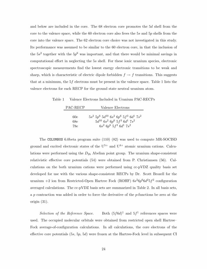
valence electrons for each RECP for the ground state neutral uranium atom.
Table 1 Valence Electrons Included in Uranium PAC-RECPs
PAC-RECP Valence Electrons
60e 5s2 5p6 5d10 6s2 6p6 5f3 6d1 7s2
68e 5d10 6s2 6p6 5f3 6d1 7s2
78e 6s2 6p6 5f3 6d1 7s2
The COLUMBUS 6.0beta program suite (110) (82) was used to compute MR-SOCISD
ground and excited electronic states of the U5+ and U4+ atomic uranium cations. Calcu-
lations were performed using the D2h Abelian point group. The uranium shape-consistent
relativistic effective core potentials (54) were obtained from P. Christiansen (56). Cal-
culations on the both uranium cations were performed using cc-pVDZ quality basis set
developed for use with the various shape-consistent RECPs by Dr. Scott Brozell for the
uranium +2 ion from Restricted-Open Hartree Fock (ROHF) 6s26p66d25f2 configuration
averaged calculations. The cc-pVDZ basis sets are summarized in Table 2. In all basis sets,
a p contraction was added in order to force the derivative of the p-functions be zero at the
origin (31).
Selection of the Reference Space. Both (5f6d)1 and 5f1 references spaces were
used. The occupied molecular orbitals were obtained from restricted open shell Hartree–
Fock average-of-configuration calculations. In all calculations, the core electrons of the
effective core potentials (5s, 5p, 5d) were frozen at the Hartree-Fock level in subsequent CI
24

Table 2 Basis Sets for Use With Uranium PAC-RECPs
cc-pVDZCore size basis
60e (7sd5p4f1g)/[5sd3p2f1g]68e (5sd4p4f1g)/[4sd2p2f1g]78e (4sd4p4f1g)/[3sd2p2f1g]
calculations. The 6s electrons, being core-like in the cc-pVDZ basis set, were also frozen.
The 6p electrons were constrained to remain doubly occupied in all references, however, sin-
gle and double excitations from the 6p shell were allowed. For U5+ only two MR-SOCISD
calculations of 15 eigenvalues each were necessary in D2h point-group symmetry to fully
characterize the ground and excited states, one for odd states, the other for even states.
States of this odd-electron system transform like the double-valued irreducible representa-
tions of the double-group. State assignment (J , L, and S) was made through analysis of
the degeneracy and parity of the computed eigenvalues.
All 91 even states arising from the 5f2 electron configuration were computed, but only
the first few low-lying odd states were listed. Dr. Scott Brozell performed the calculations
on the U4+ cation listed in Tables 5 and 6 (25). The resulting states obtained for the
even-electron U4+ system transform according to the appropriate single-valued irreducible
representations of the double-group. The spherical symmetry of the atomic calculation was
verified by investigating the degeneracy in the Ag, B3g, Au, and B3u states. Again, state
assignment (J , L, and S) was made via analysis of the degeneracy and parity of the eigen-
values. Results of the above calculations were compared with experimental measurements
of the excited states of the uranium systems compiled and available on line (17).
Results
Results for the U5+ calculations are summarized in Tables 3 and 4.
Table 3 lists the results for those calculations on U5+ using all seven references arising
from a 5f1 active space. The 2F states exhibit relative errors of roughly 10% when compared
with experiment, except for the 78 electron cc-pVDZ case, where the relative error was
25
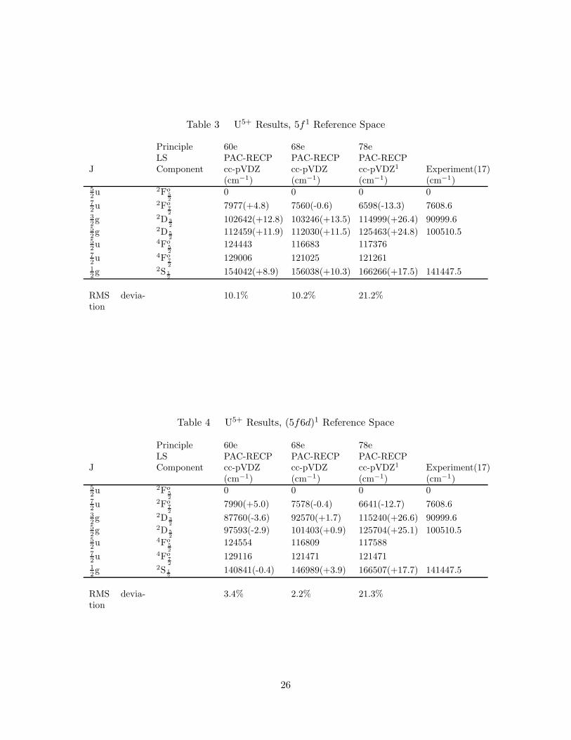
Table 3 U5+ Results, 5f1 Reference Space
Principle 60e 68e 78eLS PAC-RECP PAC-RECP PAC-RECP
J Component cc-pVDZ cc-pVDZ cc-pVDZ1 Experiment(17)(cm−1) (cm−1) (cm−1) (cm−1)
5
2u 2Fo
5
2
0 0 0 07
2u 2Fo
7
2
7977(+4.8) 7560(-0.6) 6598(-13.3) 7608.63
2g 2D 3
2
102642(+12.8) 103246(+13.5) 114999(+26.4) 90999.65
2g 2D 5
2
112459(+11.9) 112030(+11.5) 125463(+24.8) 100510.55
2u 4Fo
5
2
124443 116683 1173767
2u 4Fo
7
2
129006 121025 1212611
2g 2S 1
2
154042(+8.9) 156038(+10.3) 166266(+17.5) 141447.5
RMS devia-tion
10.1% 10.2% 21.2%
Table 4 U5+ Results, (5f6d)1 Reference Space
Principle 60e 68e 78eLS PAC-RECP PAC-RECP PAC-RECP
J Component cc-pVDZ cc-pVDZ cc-pVDZ1 Experiment(17)(cm−1) (cm−1) (cm−1) (cm−1)
5
2u 2Fo
5
2
0 0 0 07
2u 2Fo
7
2
7990(+5.0) 7578(-0.4) 6641(-12.7) 7608.63
2g 2D 3
2
87760(-3.6) 92570(+1.7) 115240(+26.6) 90999.65
2g 2D 5
2
97593(-2.9) 101403(+0.9) 125704(+25.1) 100510.55
2u 4Fo
5
2
124554 116809 1175887
2u 4Fo
7
2
129116 121471 1214711
2g 2S 1
2
140841(-0.4) 146989(+3.9) 166507(+17.7) 141447.5
RMS devia-tion
3.4% 2.2% 21.3%
26
nearly 20%, the 2D and 2S states show large relative errors of 10 to 30% with respect to
experimental measurements. The 4F states were not reported in the experimental references.
In the cc-pVDZ 78 electron RECP U5+ calculation, the ordering of the 2D and 4F states was
reversed. Without experimental measurements for the 4F states, however, the qualitatively
correct ordering of the 2D and 4F states can not be resolved at this time.
The 68 electron RECP cc-pVDZ performs nearly as well as the 60 electron core calcu-
lation overall, however, the relative error for the first excited state is much more favorable
in the 68 electron core calculation, on the order of 1% for the 68 electron core versus nearly
5% for the 60 electron core. Table 4 lists the results for those calculations on U5+ result-
ing from the 12 possible references arising from a (5f6d)1 active space. Including the five
references arising from 6d1 electronic configurations improves the relative errors in the 2D
and 2S states. Additionally, using the larger, 12 orbital active space produces consistent
ordering of the 2D and 4F states in all calculations. The 68 electron calculation results in
the lowest relative and RMS errors overall.
Table 5 lists the results for those calculations on U4+ resulting from an 5f2 reference
space, while Table 6 lists the U4+ results from a (5f6d)2 active space.
In the 5f2 active space calculation, the 68 electron core, cc-pVDZ calculation outperforms
the 60 electron core cc-pVDZ calculation in both relative and Root Mean Square (RMS)
error. The relative and RMS errors observed in the 78 electron core, cc-pVDZ calculation on
U4+ are an order of magnitude improved over the U5+ results, rivaling the results obtained
using the 68 electron core. In the (5f6d)2 active space calculation, the 68 electron core,
cc-pVDZ calculation outperforms the 60 electron core cc-pVDZ calculation in both relative
and RMS error. Using a larger active/reference space had little impact on the overall results
for the event U4+ states, all of which arise from 5f → 5f transitions. Again, the 78 electron
core results are roughly equivalent in magnitude to the 68 electron core results, both in
relative error and overall RMS error.
27
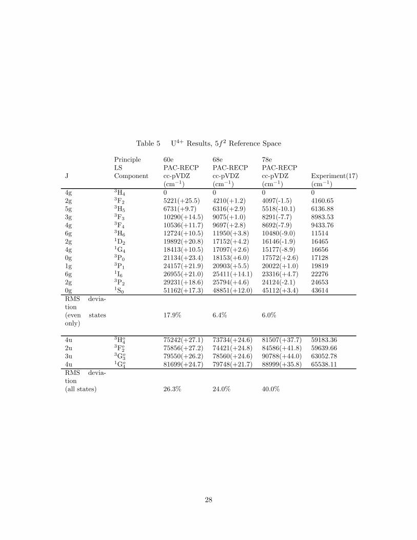
Table 5 U4+ Results, 5f2 Reference Space
Principle 60e 68e 78eLS PAC-RECP PAC-RECP PAC-RECP
J Component cc-pVDZ cc-pVDZ cc-pVDZ Experiment(17)(cm−1) (cm−1) (cm−1) (cm−1)
4g 3H4 0 0 0 02g 3F2 5221(+25.5) 4210(+1.2) 4097(-1.5) 4160.655g 3H5 6731(+9.7) 6316(+2.9) 5518(-10.1) 6136.883g 3F3 10290(+14.5) 9075(+1.0) 8291(-7.7) 8983.534g 3F4 10536(+11.7) 9697(+2.8) 8692(-7.9) 9433.766g 3H6 12724(+10.5) 11950(+3.8) 10480(-9.0) 115142g 1D2 19892(+20.8) 17152(+4.2) 16146(-1.9) 164654g 1G4 18413(+10.5) 17097(+2.6) 15177(-8.9) 166560g 3P0 21134(+23.4) 18153(+6.0) 17572(+2.6) 171281g 3P1 24157(+21.9) 20903(+5.5) 20022(+1.0) 198196g 1I6 26955(+21.0) 25411(+14.1) 23316(+4.7) 222762g 3P2 29231(+18.6) 25794(+4.6) 24124(-2.1) 246530g 1S0 51162(+17.3) 48851(+12.0) 45112(+3.4) 43614RMS devia-tion(even statesonly)
17.9% 6.4% 6.0%
4u 3Ho4 75242(+27.1) 73734(+24.6) 81507(+37.7) 59183.36
2u 3Fo2 75856(+27.2) 74421(+24.8) 84586(+41.8) 59639.66
3u 3Go3 79550(+26.2) 78560(+24.6) 90788(+44.0) 63052.78
4u 1Go4 81699(+24.7) 79748(+21.7) 88999(+35.8) 65538.11
RMS devia-tion(all states) 26.3% 24.0% 40.0%
28
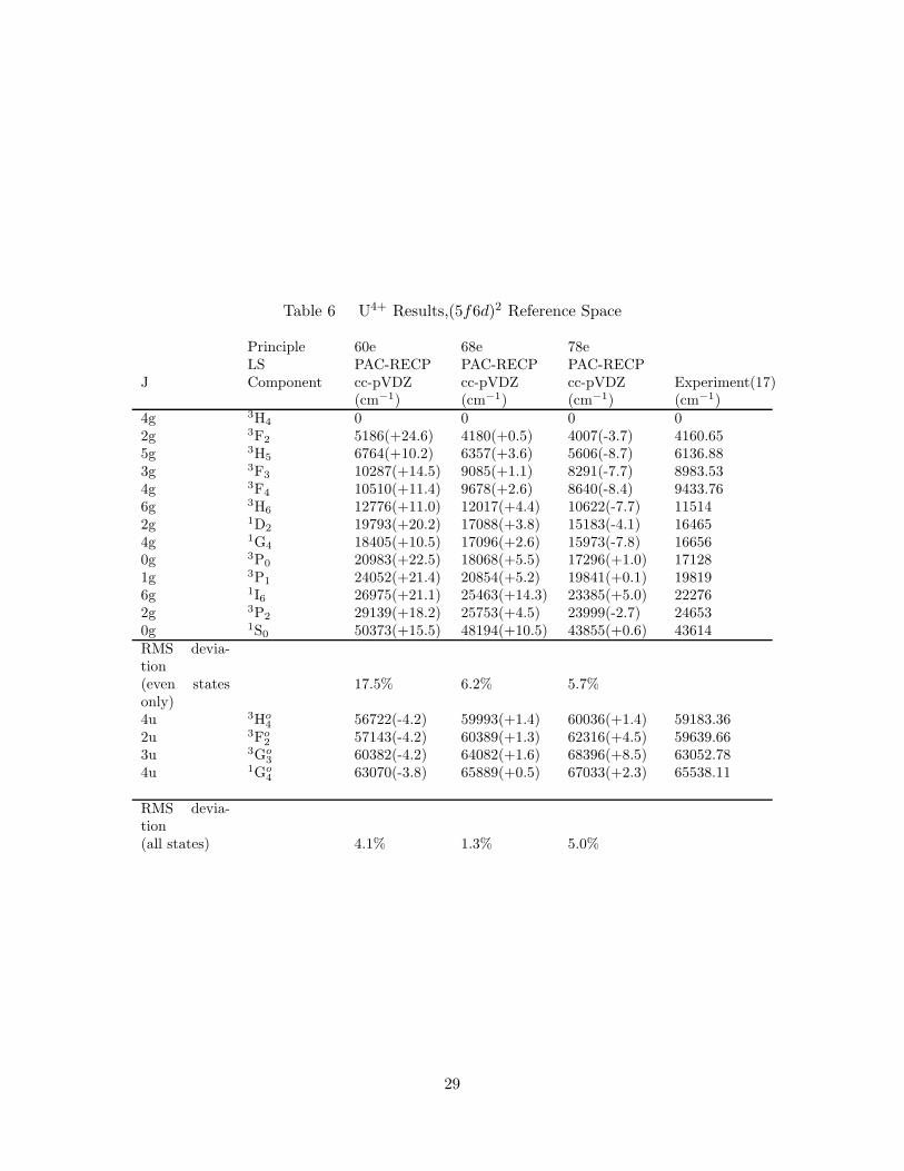
Table 6 U4+ Results,(5f6d)2 Reference Space
Principle 60e 68e 78eLS PAC-RECP PAC-RECP PAC-RECP
J Component cc-pVDZ cc-pVDZ cc-pVDZ Experiment(17)(cm−1) (cm−1) (cm−1) (cm−1)
4g 3H4 0 0 0 02g 3F2 5186(+24.6) 4180(+0.5) 4007(-3.7) 4160.655g 3H5 6764(+10.2) 6357(+3.6) 5606(-8.7) 6136.883g 3F3 10287(+14.5) 9085(+1.1) 8291(-7.7) 8983.534g 3F4 10510(+11.4) 9678(+2.6) 8640(-8.4) 9433.766g 3H6 12776(+11.0) 12017(+4.4) 10622(-7.7) 115142g 1D2 19793(+20.2) 17088(+3.8) 15183(-4.1) 164654g 1G4 18405(+10.5) 17096(+2.6) 15973(-7.8) 166560g 3P0 20983(+22.5) 18068(+5.5) 17296(+1.0) 171281g 3P1 24052(+21.4) 20854(+5.2) 19841(+0.1) 198196g 1I6 26975(+21.1) 25463(+14.3) 23385(+5.0) 222762g 3P2 29139(+18.2) 25753(+4.5) 23999(-2.7) 246530g 1S0 50373(+15.5) 48194(+10.5) 43855(+0.6) 43614RMS devia-tion(even statesonly)
17.5% 6.2% 5.7%
4u 3Ho4 56722(-4.2) 59993(+1.4) 60036(+1.4) 59183.36
2u 3Fo2 57143(-4.2) 60389(+1.3) 62316(+4.5) 59639.66
3u 3Go3 60382(-4.2) 64082(+1.6) 68396(+8.5) 63052.78
4u 1Go4 63070(-3.8) 65889(+0.5) 67033(+2.3) 65538.11
RMS devia-tion(all states) 4.1% 1.3% 5.0%
29
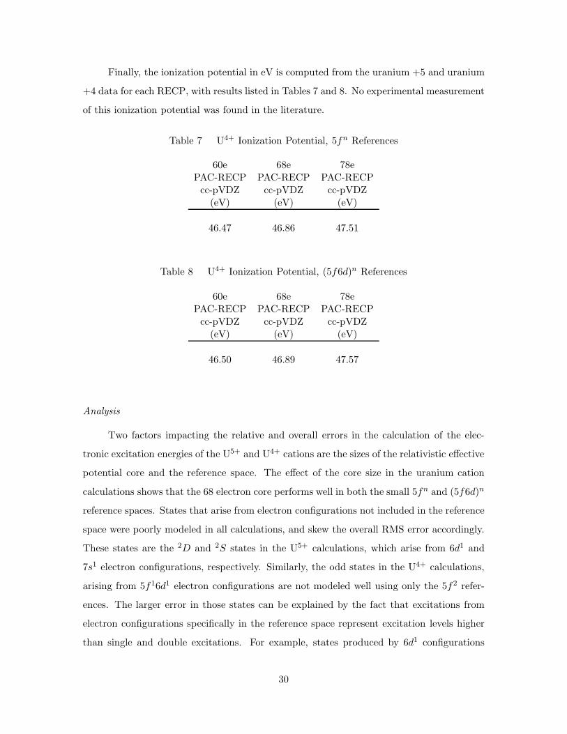
Finally, the ionization potential in eV is computed from the uranium +5 and uranium
+4 data for each RECP, with results listed in Tables 7 and 8. No experimental measurement
of this ionization potential was found in the literature.
Table 7 U4+ Ionization Potential, 5fn References
60e 68e 78ePAC-RECP PAC-RECP PAC-RECPcc-pVDZ cc-pVDZ cc-pVDZ
(eV) (eV) (eV)
46.47 46.86 47.51
Table 8 U4+ Ionization Potential, (5f6d)n References
60e 68e 78ePAC-RECP PAC-RECP PAC-RECPcc-pVDZ cc-pVDZ cc-pVDZ
(eV) (eV) (eV)
46.50 46.89 47.57
Analysis
Two factors impacting the relative and overall errors in the calculation of the elec-
tronic excitation energies of the U5+ and U4+ cations are the sizes of the relativistic effective
potential core and the reference space. The effect of the core size in the uranium cation
calculations shows that the 68 electron core performs well in both the small 5fn and (5f6d)n
reference spaces. States that arise from electron configurations not included in the reference
space were poorly modeled in all calculations, and skew the overall RMS error accordingly.
These states are the 2D and 2S states in the U5+ calculations, which arise from 6d1 and
7s1 electron configurations, respectively. Similarly, the odd states in the U4+ calculations,
arising from 5f16d1 electron configurations are not modeled well using only the 5f2 refer-
ences. The larger error in those states can be explained by the fact that excitations from
electron configurations specifically in the reference space represent excitation levels higher
than single and double excitations. For example, states produced by 6d1 configurations
30
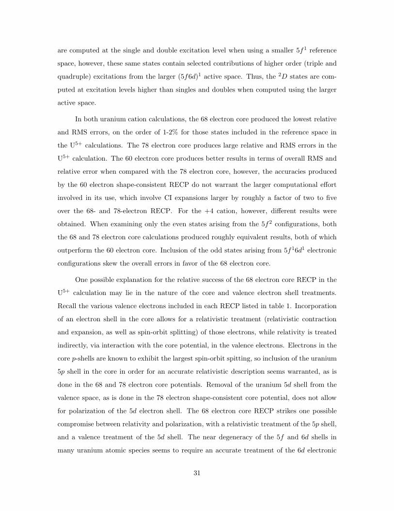
are computed at the single and double excitation level when using a smaller 5f1 reference
space, however, these same states contain selected contributions of higher order (triple and
quadruple) excitations from the larger (5f6d)1 active space. Thus, the 2D states are com-
puted at excitation levels higher than singles and doubles when computed using the larger
active space.
In both uranium cation calculations, the 68 electron core produced the lowest relative
and RMS errors, on the order of 1-2% for those states included in the reference space in
the U5+ calculations. The 78 electron core produces large relative and RMS errors in the
U5+ calculation. The 60 electron core produces better results in terms of overall RMS and
relative error when compared with the 78 electron core, however, the accuracies produced
by the 60 electron shape-consistent RECP do not warrant the larger computational effort
involved in its use, which involve CI expansions larger by roughly a factor of two to five
over the 68- and 78-electron RECP. For the +4 cation, however, different results were
obtained. When examining only the even states arising from the 5f2 configurations, both
the 68 and 78 electron core calculations produced roughly equivalent results, both of which
outperform the 60 electron core. Inclusion of the odd states arising from 5f16d1 electronic
configurations skew the overall errors in favor of the 68 electron core.
One possible explanation for the relative success of the 68 electron core RECP in the
U5+ calculation may lie in the nature of the core and valence electron shell treatments.
Recall the various valence electrons included in each RECP listed in table 1. Incorporation
of an electron shell in the core allows for a relativistic treatment (relativistic contraction
and expansion, as well as spin-orbit splitting) of those electrons, while relativity is treated
indirectly, via interaction with the core potential, in the valence electrons. Electrons in the
core p-shells are known to exhibit the largest spin-orbit spitting, so inclusion of the uranium
5p shell in the core in order for an accurate relativistic description seems warranted, as is
done in the 68 and 78 electron core potentials. Removal of the uranium 5d shell from the
valence space, as is done in the 78 electron shape-consistent core potential, does not allow
for polarization of the 5d electron shell. The 68 electron core RECP strikes one possible
compromise between relativity and polarization, with a relativistic treatment of the 5p shell,
and a valence treatment of the 5d shell. The near degeneracy of the 5f and 6d shells in
many uranium atomic species seems to require an accurate treatment of the 6d electronic
31
excitations, which can be facilitated by freeing the 5d shell from the core and into the valence
electron space.
The similar performance of the 78 and 68 electron cores in the even-state U4+ calcu-
lations seems to counter the argument presented above. One possible source of this result is
the fact that in this core potential treatment, there are no core-valence interactions possible,
so the shape-consistent core potential method does not include any way for the core region
to polarize. Thus, while the 68 electron core allows polarization of the 5d electrons, while
only incorporating relativistic effects indirectly, through interaction with the core potential,
the 78 electron core allows a relativistic treatment of the 5d electrons, but no relaxation
of the 6d shell to occur. One possible explanation of the observed results is that these
treatments are roughly the same magnitude, and that a higher order description of the
core-valence interaction may be necessary to resolve the near degeneracy in the 68 and 78
electron core results. The fact remains, however, that the 78 electron core calculations rep-
resent a lower computation cost, and give reasonably accurate results, in the even-state U4+
calculations. It should be noted that event the 2% RMS error obtained in the 68-electron
RECP calculation on U5+ is poor when compared with the precision obtainable in exper-
imental measurements photoluminenscence spectroscopy. The presence of a trend may be
established by examining the U3+ and U2+ cations. The similiar performance in the 68
and 78 electron cores does not carry over to the odd-states in the uranium +4 cation above
the 4u state. This could be a result of significant contribution of the 7s references to the
2u states and above, which are not present in the reference spaces examined here. Marked
improvement in the odd-states is observed in going from the 5f2 to the (5f6d)2 reference
space calculations.
Overall, applying Christiansen et al shape-consistent relativistic effective core poten-
tials in MR-SOCISD calculations of the ground and excited states of U5+ and U4+ ions shows
that the 68 electron PAC-RECP, along with a cc-pVDZ basis set, yields relative errors with
respect to experimental measurements of 1 to 3% of experiment for each calculated state,
part of which may be due to a fortuitous cancellation of error based on analysis of results
obtained using double-ζ quality basis sets. The lowest relative errors in excitation energies
were achieved when the reference space included all the electron configurations spawning
32

the states of interest. Inclusion of the spin-orbit interaction is crucial in these calculations,
as the lowest energy electronic transitions in U5+ and U4+ arise from 5f → 5f transitions.
33
III. The COLUMBUS-based DFT/MRCI Model
This chapter details the theoretical basis underlying the DFT/MRCI model, as well as de-
tailed analysis of critical aspects of the model. The implementation, testing, and validation
of the DFT/MRCI model is presented in detail, followed by applications of the model to
various atomic and molecular systems and a discussion of the results obtained.
Theory
The theoretical foundation behind this hybrid DFT/MRCI model lies in the union
of two distinct theoretical approaches to quantum chemistry: the Kohn-Sham approach to
DFT and GUGA CI.
Non-relativistic Quantum Theory. The main goal of non-relativistic computational
quantum chemistry revolves around the need to solve, exactly if possible, the time dependent
Schrodinger wave equation for many-electron atoms and molecules. The time dependent
equation is (35:211)
In Equation 5, H is the Hamiltonian operator, while Ψ (~x1, ~x2, . . . , ~xn) represents an
N electron wave function. Each ~xi represents the electronic coordinates of the ith electron.
For time independent states, the Schrodinger wave equation reduces to (35:245) (106:26-29)
(127:40)
Hψ (~x1, ~x2, . . . , ~xn) = Eψ (~x1, ~x2, . . . , ~xn) . (25)
This representation assumes the Born-Oppenheimer approximation is valid, where the nu-
clear and electronic wave functions are uncoupled and treated separately. In this approxima-
tion, the electronic Hamiltonian operator, H can be written using atomic units (127:41-42)
(106:155-156) as
H = −1
2
N∑
i=1
∇2i −
N∑
i=1
M∑
a=1
Za
ria+
1
2
N∑
i=1
N∑
j=1
1
rij. (26)
where ria is the distance between the electron i and nucleus a, Za is the charge on the
a-th nucleus, and rij is the distance between electron i and electron j. The first term is
the electronic kinetic energy operator, the second term is the electronic-nuclear attraction
potential energy, while the last term represents the electron-electron repulsion potential
energy.
34
One approach to solving Equation 25 is to expand the electronic wave function, ψ
in a product of N independent, one-electron wave functions, ψ =N∏
i=1ϕi(~xi), with each ϕi
is a one-electron wave function called an orbital. The Pauli Exclusion Principle requires
that this wave function be antisymmetric upon the exchange of any two electrons. A Slater
determinant is one useful mathematical construct that results in a properly antisymmetric
wave function, defined by
Ψ =1√N !
∣
∣
∣
∣
∣
∣
∣
∣
∣
∣
∣
∣
ϕ1(~x1) ϕ2(~x1) · · · ϕN (~x1)
ϕ1(~x2) ϕ2(~x2) · · · ϕN (~x2)...
.... . .
...
ϕ1(~xn) ϕ2(~xn) · · · ϕN (~xN )
∣
∣
∣
∣
∣
∣
∣
∣
∣
∣
∣
∣
, (27)
where each determinant represents a particular electron configuration in the many-electron
system (78). Wave functions can be formed from either a single Slater determinant, as is
the case in the Kohn-Sham or Hartree-Fock approximations, or by linear combinations of
Slater determinants.
The Hartree-Fock Approximation. The Hartree-Fock method finds the set
of orthogonal molecular orbitals, that, when antisymmetrized using a single-determinant,
yields the lowest possible energy. The Hartree-Fock approximation is a variational method,
in that the Hartree-Fock energy obtained is guaranteed to be bounded from below by the
exact energy of the system. The Hartree-Fock approximation is a mean-field approximation,
where each electron experiences the average field of all other electrons, with the wave func-
tion written as a single Slater determinant of one-electron orbitals. The difference between
the exact, non-relativistic energy and the Hartree-Fock energy is defined as the correlation
energy.
Correlation energy, which comes from two sources, is not modeled by the Hartree-Fock
approximation by definition. The first source of correlation energy, non-dynamic correlation,
is a result of the failure of the single Slater determinant model to adequately model the
correlation between electrons with opposite spins. The second source of correlation energy,
dynamic correlation, is from electron-electron coulombic interactions not modeled accurately
by the mean-field approximation (127:231-232) (106:284-288) (37:541-542).
35

The Hartree-Fock energy is given by (37:37-96) (127:108-151) (106:269-307)
EHF =
N∑
i=1
(
i| h |i)
+1
2
N∑
i=1
N∑
j=1
[(ii|jj) − (ij|ji)], (28)
where the first term includes the one-electron kinetic and potential energies given by
(
i| h |i)
=∑
a
∫
ϕ∗i (~x1)
(
−∇2 − Za
ria
)
ϕi(~x1)d3x1. (29)
The second term the electron-electron Coulomb repulsion, modeling the local interaction
between two charge densities, given by the integral (127:113)
(ii|jj) =⟨
ϕi(~x1)|Jj |ϕj(~x2)⟩
=
∫
|ϕi(~x1)|21
r12|ϕj(~x2)|2 d3x2d
3x1, (30)
where |ϕi(~x1)|2 is the probability density for the ith electron.
The third term in Equation 28 the electron-electron exchange interaction energy, which
is a non-local interaction between an electron at a particular position and all the other
electrons with identical spin over all space. This term correlates the motions between
electrons with parallel spin. The energy is given by the integral (127:113)
(ij|ji) =⟨
ϕi(~x1)|Kj |ϕj(~x2)⟩
=
∫
ϕ∗i (~x1)ϕj(~x1)
1
r12ϕ∗
j(~x2)ϕi(~x2)d3x2d
3x1. (31)
In operator form, the Hartree-Fock equation is given by (127:114)
Fϕi(~x1) =
h(~x1) +N∑
j 6=i
Jj(~x1) − Kj(~x1)
ϕi(~x1) = εiϕi(~x1), (32)
where F is the Fock operator defined in Equation 32, and Jj is defined by (127:113)
Jj(~x1)ϕi(~x1) =
[∫
ϕ∗j (~x2)
1
r12ϕj(~x2)d
3x2
]
ϕi(~x1) (33)
and Kj is defined by (127:113)
Kj(~x1)ϕi(~x1) =
[∫
ϕ∗j (~x2)
1
r12ϕi(~x2)d
3x2
]
ϕj(~x1). (34)
36
This molecular orbital basis representation of the Fock operator is diagonalized, and the
total Hartree-Fock energy is then given by
E0 =N∑
i
⟨
i|h|i⟩
+1
2
N∑
i
N∑
j
〈ij||ij〉, (35)
with 〈ij||ij〉 given by⟨
i|Jj |i⟩
−⟨
i|Kj |i⟩
(36)
Correlation effects can contribute roughly 1 eV (23 kcal/mol) to the total electronic
energy per electron pair (112). An accurate treatment of electronic correlation is critical
in order to perform meaningful comparisons between theoretical and experimental spectra.
The Kohn-Sham approach to DFT is an elegant method for computing dynamic correlation
energy using a single-determinant model.
The Kohn-Sham Approach to DFT. An alternative approach to solving Equation
25 using an electronic wave function is to use the electron density in two famous theorems.
Hohenberg and Kohn proved that an exact solution to Equation 25 could be obtained using
the electron density (70).
The first Hohenberg-Kohn theorem states that the potential is a unique functional
of the density, neglecting a trivial constant factor. This simple theorem proves that the
electron density completely determines the external potential, which, in turn, completely
specifies the Hamiltonian. Hohenberg and Kohn’s second theorem proves that this energy
functional of the electron density is a minimum only when the exact ground-state density
is used. Moreover, the only part of the energy functional that is system dependent is the
external potential, Vext (~r). For atomic and molecular systems, this external potential is 1rij
.
This implies that there exists a universal kinetic energy and electron-electron interaction
functional, valid for any electronic system. Thus,
E0 [ρ] =
∫
Vext (~r)ρ (~r) d~r + FHK [ρ] ,
FHK [ρ] = T [ρ] + Vee [ρ] .
(37)
37
In equation 37, T is the kinetic energy density functional, and Vee is the electron-electron
interaction potential. Here, Vee [ρ] can be split into classical and non-classical terms,
Vee [ρ] =1
2
∫
ρ (~r1) ρ (~r2)
|~r1 − ~r2|d~r1d~r2 + Vnon−classical [ρ] . (38)
Hohenberg and Kohn’s second theorem outlines a procedure for finding this exact ground
state density. The theorem states that the exact energy can be determined via the variational
principal, and that the exact density yields the lowest, exact energy. The only drawback
is that the universal functional, FHK [ρ], is not known. However, the existence of such a
functional is guaranteed, and once it is found, the non-relativistic Schrodinger wave equation
can be solved exactly for the ground state electron density. While the Hohenberg-Kohn
theorems proved the existence of a unique, exact energy functional of the electron density
which would variationally yield the exact ground state energy of an atom or molecule, it
did not proscribe a method for finding this density. In 1965, Kohn and Sham introduced a
set of self-consistent equations which provided a means for computing the density efficiently
(79), very similar to the linear combination of atomic orbital method of Roothaan equations
(114) (115) for the Hartree-Fock model. The Kohn-Sham approach introduced a fictitious,
non-interacting system built from one-electron orbitals. However, unlike the Hartree-Fock
model, where the one-electron orbitals are variationally optimized to yield the lowest total
energy, the Kohn-Sham orbitals are chosen in order to reproduce the exact ground state
density. In the Hartree-Fock approximation, the kinetic energy can be exactly written as
THF = −1
2
N∑
i=1
〈ϕi|∇2 |ϕi〉 , (39)
exact because of the exact treatment of the non-local exchange potential in the Hartree-Fock
formulation. In the Kohn-Sham approach, a non-interacting reference system is introduced,
creating an effective Hamiltonian given by
HKS =−1
2
N∑
i=1
∇2 +
N∑
i=1
Vs (~ri), (40)
38
where Vs (~ri) is an effective, local potential. The Kohn-Sham approach then consists of
choosing Vs (~ri) in order to yield the exact, ground state density from
ρ (~r) =N∑
i=1
fi |ϕKS (~r)|2 . (41)
Here, the fi are Kohn-Sham orbital electron occupations numbers, while the φKS are the
Kohn-Sham molecular orbitals. The main idea behind the Kohn-Sham approach is to take
the universal functional of Hohenberg and Kohn, FHK in Equation 37, and approximate it
by separating out the energy of a non-interacting system, which accounts for the majority
of the total energy of a system. Thus,
FHK [ρ] = Ts [ρ] + Ec [ρ] , (42)
where Ts [ρ] represents the strictly local kinetic energy functional of a non-interacting sys-
tem of electrons with density ρ (~r), and Ec [ρ] is defined as the exchange and correlation
energy of the interacting system of electrons. Ec[ρ] includes the kinetic energy of the inter-
acting electronic system, as well as Coulomb electron-electron correlation and non-classical
fermionic exchange. All these density functionals are all local, in that electron density at a
point in space can only affect the energy in a small region of space. The fermionic exchange
interaction described earlier is a non-local interaction, in that the electron density over all
space affects the energy locally. This non-local aspect of the exchange interaction is a major
challenge in the development of approximate density functionals, and it is the foundation
of the Taylor expansion approach in exchange functional development.
Varying the energy functional with respect to the density yields the Kohn-Sham equa-
tions (79){
−1
2∇2 + [ϕ (~r) + µxc [ρ]]
}
ϕKSi (~r) = εiϕ
KSi (~r) , (43)
with
ϕ(~r) = v(~r) +
∫
ρ(~r)
|~r − ~r′ |d~r
′
. (44)
Here, v(~r) is the Coulomb potential, and µxc[ρ] is the correlation (and interacting kinetic
energy) density functional. Together, ϕ(~r) + µxc[ρ] form an effective potential, veff (~r).
39
The main reason for the popularity of DFT as a computational tool today is that
the same computational code developed and optimized for HF Self-Consistent Field (SCF)
calculations could be immediately used for DFT calculations, the only difference being
the need for evaluation of integrals over the correlation density functional. This allows
introduction of electron-electron correlation to be included in a calculation with nearly
the same computational cost as a Hartree-Fock calculation. DFT provides an inexpensive
method to compute electron-electron dynamic correlation energy using an efficient one-body
correlation operator.
A number of approximations to the universal functional give by Equation 42 exist,
with the most successful based upon numerical fits to quantum mechanical Monte Carlo
calculations on the ground state of a homogeneous electron gas by Ceperley and Alder (30).
Accurate hybrid functionals have also been developed that include some mixture of exact
HF exchange, including B3LYP (12), PBE (102), and PBE0 (2).
More accurate modeling the non-local aspects of the exchange operator, through the
inclusion of higher order Taylor expansions of the electron density, also known as Jacob’s
Ladder (87) (131), has lead to the development of modern density functionals . Local
density functionals involve only the electron density, while a GGA functional uses both the
electron density and the gradient of the electron density. Modern functionals incorporate
the Lapacian of the electron density, resulting in meta-GGA density functionals.
Configuration Interaction and the Graphical Unitary Group Approach. A concep-
tually simple and popular method to compute electron-electron correlation energy is CI.
In a CI calculation, the many-electron wave function is expanded in a series of states that
differ from the ground state by exciting one or more electrons from a ground-state occupied
molecular orbital to an unoccupied virtual orbital. Including all states that differ from the
ground state by a single excitation is known as Configuration Interaction Singles (CIS),
while including all possible single and double excitations is known as CISD. A FCI calcu-
lation is obtained if all possible excitations were included in the expansion. In the limit of
a complete basis set, the full CI calculation yields the exact solution to the many-electron,
non-relativistic Schrodinger equation. The CI approach does not require additional physics
40
beyond the one-electron orbital model of Hartree-Fock, it simply corrects for deficiencies in
the orbital basis chosen.
The CI wave function is written
Ψ = c0Ψ0 +∑
a,i
cai Ψai +
∑
a,b,i,j
cabij Ψab
ij +∑
a,b,c
ca,b,cijk Ψabc
ijk + · (45)
The first term is the HF wave function, the second term is a sum over all singly excited
states from the HF ground state, the third term consists of a sum over all doubly excitations,
and so on. Additionally, the expansion coefficients, cabc·ijk·, are variationally optimized. In
practice, this CI expansion must be truncated at some point, typically at single and double
excitations. Brillouin’s theorem (127:233-236) proves that there is no direct mixing between
the HF ground state and singly excited states. However, the HF ground state does mix
with the doubly excited states, which in turn couples to the singly excited states. The first
logical place to truncate the CI expansion in order to obtain an improvement of the HF
wave function is to truncate Equation 45 at single and double excitations.
The CISD method, while conceptually simple, can be very computationally demand-
ing. It is known to exhibit slow convergence to the exact total electron correlation energy. In
an N -electron system using K basis functions, the number of all possible double excitations
is given by (127:232) (37:543).
N
2
2K −N
2
. (46)
The number of configurations involved in the CISD method scales roughly as (2K)2N2 . An
additional drawback to truncated CI expansion calculations is the fact that the truncation is
not size extensive. A size extensive calculation scales linearly with the number of component
parts of the system. For example, a size extensive calculation on the system AB, and two
calculations on A and B separately provide the same accuracy both on the combined system
as well as the individual component parts. Size extensivity is important when calculating
certain molecular properties, such as dissociation energies. One result of non-size extensivity
in truncated CI calculations is that a calculation on the system AB contains excitations not
41
present in the component calculations on either A or B separately. Full CI calculations are
size extensive, however, they are only possible using relatively small atomic or molecular
systems with modest basis sets.
CI calculations provide a conceptually simple, yet computationally demanding way
to compute both dynamic and non dynamic electron correlation energy. CIS calculations
can not change the HF ground state, as a result, they do not model dynamic electron
correlation. They do, however, model some of the multi determinant nature of the electronic
wave function and can model some of the non dynamic electron correlation energy. CISD
calculations model a portion of both dynamic and non dynamic electron correlation.
Two different approaches to performing CI calculations exist, determinant-based CI
and GUGA-based CI. The first approach uses computes the complete CI Hamiltonian in
a Slater determinant basis, where each Slater determinant is formed through excitation of
electrons from some reference determinant or determinants. It is relatively straightforward
to generate arbitrary excitation levels within a determinant basis, up to the full CI exci-
tation levels of N excitations in an N electron system. This is achieved through simple
substitution of virtual for occupied orbitals in the appropriate Slater determinant. Once
the CI Hamiltonian is formed in the determinant basis, it is stored, either in memory or on
disk, and then diagonalized. In general, Slater determinants are not spin eigenfunctions, and
linear combinations of Slater determinants must be formed in order to construct states with
well-defined spin multiplicity. This approach faces disk access bottlenecks, as large numbers
of one- and two-electron integrals necessarily need to be accessed, essentially randomly, in
order to construct the CI Hamiltonian. Once constructed, this Hamiltonian must be stored
in some fashion in order to apply some large, sparse, symmetric matrix diagonalization rou-
tine in order to find the eigenvalues. These requirements can become quite demanding for
large molecules, large basis sets, or both (120:86-88).
One way around this limitation is to use a direct method. In a direct method, the
appropriate Hamiltonian matrix elements are constructed as needed, then discarded. This
can reduce the disk access requirements, in that a relatively small subset of information
need be stored. An effective way to determine which Hamiltonian matrix elements need
42
to be computed for the eigenvalue of interest, and from these, the one- and two-electron
integrals and the coupling coefficients involved (120:86-88).
The GUGA direct CI (113) (52) approach accomplishes just that. The technical details
of GUGA are examined in detail in the literature (119) (120) (121).
Using unitary group techniques, a compact representation of the CI orbital basis is
possible in the form of a Distinct Row Table (DRT). Using this DRT, one can efficiently
construct all possible Configuration State Functions (CSFs) arising from some reference
electronic configuration, or set of reference configurations. CSFs, which are spin eigenfunc-
tions, can be efficiently defined in terms of molecular orbitals using the DRT, taking into
account both spin-multiplicity and spatial symmetry. Not only does the DRT allow compact
and efficient organization of the orbital basis functions into CSFs, it also provides, through
the graphical representation, insight into the structure of the CI Hamiltonian. Figure 1
(122) shows the graphic depiction of a distinct row table for a MR-CISD calculation. The
reference CSFs are shown in red. The MR-CISD graph is broken up into two distinct re-
gions, internal (active and inactive), and external spaces. The internal space consists of
those orbitals that are occupied in the reference configurations. Inactive orbitals are doubly
occupied in all references, while active orbitals can be either doubly, singly, or unoccupied
in the reference space. External orbitals, or virtual orbitals, are unoccupied in the reference
space. The structure of the graph of the external space is relatively simple, and indepen-
dent of the size of the number of external orbitals. The MR-CISD graph is arranged in this
fashion due to the regular structure of the external space, and inactive internal space (122).
43

Figure 1 Distinct Row Table Graph for Multi Reference Single and Double ExcitationConfiguration Interaction Expansion (122)
44
The Unitary Group and the Repartitioning of the Hamiltonian. The utility of
the GUGA approach so far has been to compactly and efficiently index all possible CSFs
arising from some arbitrary excitation level within an orbital basis. Truncation of this CI
expansion is easily achieved, removing individual CSFs, groups of CSFs, or even entire
excitation levels. The real power behind the GUGA approach lies in its ability to describe
the coupling between CSFs, allowing the efficient computation of the CI Hamiltonian matrix
elements between CSFs (120:65-69).
There is a direct correspondence between the CI Hamiltonian matrix elements between
CSFs and the matrix elements of the unitary group generators, Eij . These unitary group
matrix elements can be constructed from generator operators, which satisfy the commuta-
tion relation (120:69-70) (123)
[
Eij , Ekl
]
= δjkEil − δilEkj, (47)
corresponding to
EijEkl − δjkEil = EklEij − δilEkj. (48)
This generator operating on a Configuration State Function (CSF) has the effect of moving
an electron from orbital j to orbital i without changing the overall spin-state. This is useful
because the generators of the unitary group satisfy the same commutation relation as the
second-quantization substitution operators (124),
Eij = X†iαXjα + X
†iβXjβ, (49)
where the X† are creation operators, and the X are annihilation operators, creating or
annihilating an electron in spatial orbital i or j with spin α or β. In second-quantization
form, the Hamiltonian is (120:65-66)
H =∑
ij
∑
σ
hijX†iσXjσ +
1
2
∑
ijkl
∑
στ
[ij; kl] X†iσX
†kτ Xlτ Xjσ, (50)
where
hij = 〈i |h| j〉 , (51)
45
and
[ij; kl] =
⟨
i (1) k (2)
∣
∣
∣
∣
1
r12
∣
∣
∣
∣
j (1) l (2)
⟩
. (52)
In Equation 50, σ and τ run over electron spin states α and β.
It is useful to repartition the CI Hamiltonian so that states are described not relative
to the vacuum state, but instead states are described relative to some reference state or
states. A particularly useful choice is to select a reference occupancy, µk, corresponding to
the most common orbital occupancy in the reference space. A new set of modified one- and
two-body unitary group operators can be defined by (120:66-69)
Fij = Eij − µiδij , (53)
fij,kl = eij,kl− (54)(
µiδijEkl + µkδklEij − µiµkδijδkl
)
+ (55)
1
2
(
µiδilEkj + µkδkjEil − µiµkδilδkj
)
+ (56)
1
2(2 − µi) δijδklδkj . (57)
This definition removes reference occupancy contributions from terms in Equation 50. In-
troducing a modified Fock operator (120:68)
u = h+∑
k
µk
(
Jk − 1
2Kk
)
, (58)
with Jk and Kk being the normal Coulomb and exchange operators. Using the definitions
presented in equations 53 through 58, along with modified one-electron integrals defined by
(120:68-69)
uij = hij +∑
k
µk
(
[ij; kk] − 1
2[ik; kj]
)
, (59)
one can recast the second quantized form of the Hamiltonian, Equation 50, into a reparti-
tioned form,
H = E0 +∑
ij
uijFij +1
2
∑
ijkl
[ij; kl] fij,kl. (60)
46
In this repartitioned form, the reference energy, E0 is given by
E0 =1
2
∑
i
[µi (hii + εi) − µi (2 − µi) gii] , (61)
where gij = [ii; jj] − 12 [ij; ji] and εi = uii = hii +
∑
k µkgik.
Matrix Elements of the Repartitioned Hamiltonian. Now that the reparti-
tioned Hamiltonian has been suitably defined in Equation 60, the next step in order to
perform a GUGA based CI calculation is to compute the matrix elements between arbitrary
CSFs.
Matrix elements between two CSFs, m and m′, are obtained from (124)
⟨
m′∣
∣
∣H∣
∣
∣m⟩
=∑
ij
∑
σ
hij
⟨
m′∣
∣
∣Eij
∣
∣
∣m⟩ 1
2
∑
ijkl
∑
στ
[ij; kl]⟨
m′ |eij,kl|m⟩
, (62)
with Eij the unitary group generator, and eij,kl given by
EijEkl − δjkEil = eij,kl = ekl,ij. (63)
The matrix elements of the generator Eij and eij,kl are coupling coefficients between two
CSFs. For diagonal, or weight, generators, Eii, the matrix elements are particularly simple,
given by (124).⟨
m′ |Eii|m⟩
= δm′mni (m) . (64)
Here, ni(m) is the occupancy of orbital i in the CSF m. The one-body raising and lowering
generators are adjoint, Eij = E†ji, resulting in (120:70) (124)
⟨
m′∣
∣
∣Eij
∣
∣
∣m⟩
=⟨
m∣
∣
∣Eij
∣
∣
∣m′⟩
. (65)
Because of 65, matrix elements over the raising generators, Eij need only be computed. An
additional identity⟨
m′∣
∣
∣Eij
∣
∣
∣m⟩
= 0, (66)
47
further simplifies things, provided i < j and m′ ≥ m. Outside of the range (i, j), the two
CSF orbital occupancies and spin coupling must coincide. Inside the range (i, j), a loop in
the DRT graph is formed. Vertices of the m and m′ branches of the loop must be related
by (120:70-72) (124)
N ′k = Nk + 1 (67)
and
S′k = Sk ± 1
2, (68)
in order for a non-vanishing matrix element, 〈m′ |Eij |m〉 to be non-vanishing, where Nk and
Sk are the electron occupation and spin-multiplicity at the k-th level of the DRT respectively.
This limits the possible relationships between two vertices in the DRT graph at each level k.
The value of the matrix element can be constructed from the product of individual segment
values within the loop (120:73) (124)
⟨
m′ |Eij |m⟩
=∏
k=(i,j)
ω(
Qk; d′kdk,∆bk, bk
)
. (69)
Here, Qk is a segment type symbol, with possible values Qk = W, R, L, R,L,R, or L. By
defining Tk = (Qk; d′kdk,∆bk) as a segment shape symbol, one obtains (120:73) (124)
⟨
m′ |Eij |m⟩
=∏
k=(i,j)
ω (Tk, bk) , (70)
where Tk is now dependent only on the shape of the segment interaction, and all segment
interactions with the same shape are equivalent. These Tk are one-body segments. The
end result is that the GUGA CI matrix element between two interacting CSFs depends
only on the difference in electron occupation and spin-multiplicity over a limited range of
orbitals. In the graphical representation, these interacting CSFs form a loop over a narrow
range of levels on the DRT, with a limited number of possible arc interactions. The CI
matrix element can be constructed as a factored product of separate loop interactions over
the range of orbitals where the two CSFs differ, either by occupation, spin-multiplicity, or
both. All possible one body loop segment shapes are shown in Figure 2. Step numbers
48
are shown in red, along with relative b values. The loop values are also listed below each
segment shape (124).
A similar treatment of the matrix elements of the two-body generators yields (120:76-
86) (124)⟨
m′ |eij,kl|m⟩
=∏
p∈S1
ω (Tp, bp)∑
x=0,1
∏
p∈S2
ωx (Tp, bp) , (71)
where S1 = (i, j) ∪ (k, l) − S2 and S2 = (i, j) ∩ (k, l). S1 is the non-overlapping region
between the two CSFs, while S2 is the overlapping region. S1 and S2 range over i, j,
k, and l, inclusive. Again, the result is that the matrix element can be factored into
shape dependent factors, which are equivalent as long as segment shapes are the same, and
level dependent factors, bp. Through a careful definition of the various Tk segment shape
symbols, matrix elements over one-body and two-body unitary group generators can be
computed. These matrix elements are then the coupling coefficients between CSFs in both
the Hamiltonian and the repartitioned Hamiltonian, and facilitate an efficient, loop-driven
(24) direct CI calculation (120:86-96) (124). All non-zero contributing loop segment shapes
to the CI Hamiltonian are shown in Figure 3.
49
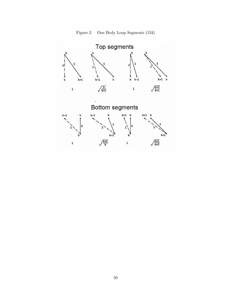
Figure 2 One Body Loop Segments (124)
50
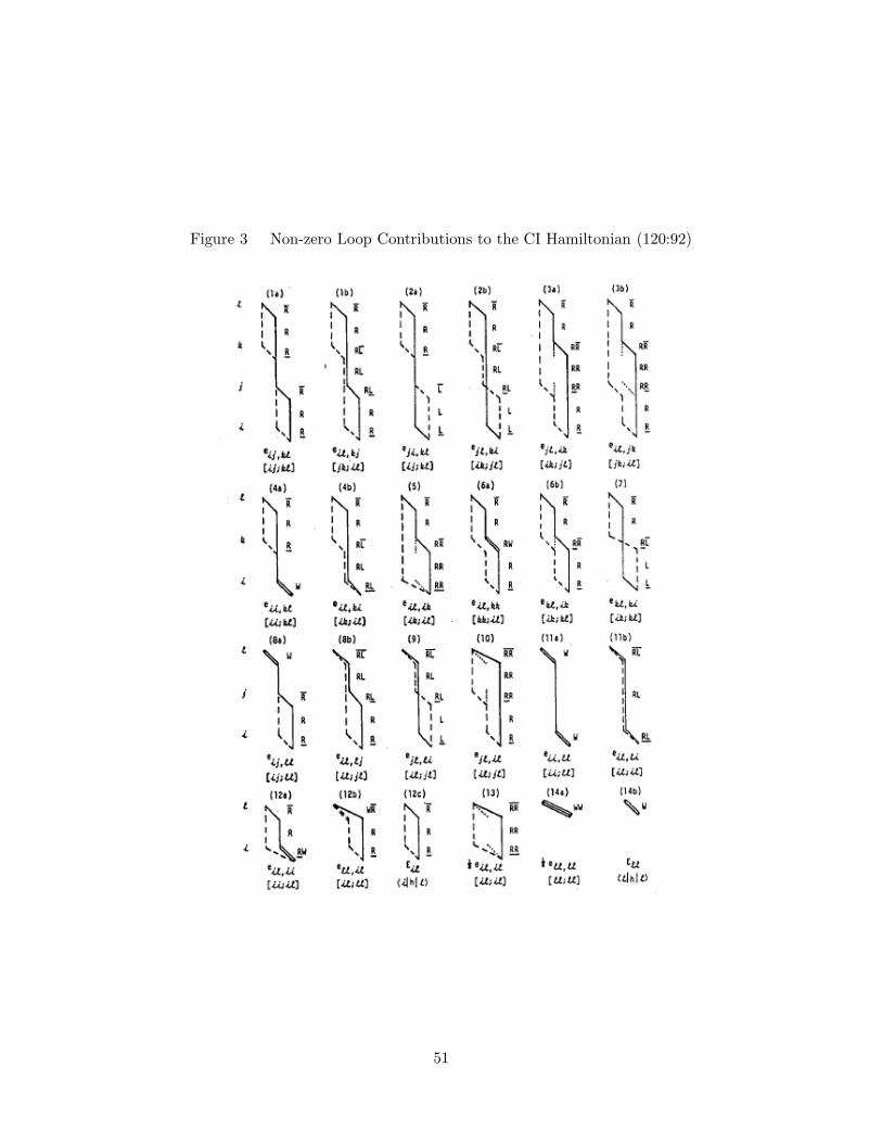
Figure 3 Non-zero Loop Contributions to the CI Hamiltonian (120:92)
51
Hybrid DFT/MRCI Model. While DFT accounts for dynamic electron-electron
correlation via an approximate correlation density functional, it has difficulty in modeling
atomic and molecular systems with significant multi determinant character. This is not
necessarily a failing of the theory, which, in principle, is exact if the exact universal den-
sity functional was known and used, but a failing of the approximate density functionals
developed to date.
One possible way to model this multi reference, non-dynamic electron-electron corre-
lation was proposed by Grimme (62). His approach was to use the Kohn-Sham molecular
orbitals generated by a DFT calculation as the expansion basis for a relatively small CIS
calculation. His idea was that the CI calculation would provide a way to compute the multi
determinant non-dynamic correlation, while the single reference DFT calculation modeled
the dynamical electron-electron correlation via the approximate correlation density func-
tional.
By performing CIS in his first paper, and later CISD with Walteske (63), Grimme
was able to compute electronic excitation energies of several systems known to have signifi-
cant non-dynamic electron correlation accurately when compared with experiment and more
traditional, wave function based approaches. During the construction of the CI Hamilto-
nian, Grimme and Waletske construct an effective DFT/CI Hamiltonian using the following
construction for diagonal matrix elements (63)
〈ωw|HDFT − EDFT |ωw〉 = 〈ωw|H − EHF |ωw〉 −nexc∑
c
FHFcc − FKS
cc +
nexc∑
a
FHFaa − FKS
aa +1
nexc
nexc∑
a
nexc∑
c
pJ (aa|cc) − p [N0] (ac|ac) , (72)
where FKSij is the matrix element of the Kohn-Sham effective Hamiltonian given by
FKSij = hij + (i|Vc (ρ) j|) +
∑
k
nk (ij|kk) , (73)
and ω and w represent spin-coupling pattern and spacial occupation vector, respectively.
Grimme and Waletske replace the HF orbitals with their Kohn-Sham counterparts,
then they scale the two electron contributions to the excitation energy by empirically de-
52
termined constants, pj and p[N0]. According to their research, the scale factor pJ depends
on the amount of exact HF exchange used in the computation of the Kohn-Sham orbitals,
and is given in this case by
pJ = 1 − xHF , (74)
where xHF is the amount of exact HF exchange used in the DFT calculation, taking the
value of zero if no Hartree-Fock exchange was included, and one if no exchange functional
was used. The second parameter, p[N0], depends on the number of open shells, N0 in the
state |ωw〉. They observed a systematic increase in p[N0] as the number of open shells
increased in their calculations, and they assumed a linear relationship between p[N0] and
N0. For singlet states, they assumed the relationship
p[N0] = 1p[0] +N10α, (75)
while for triplet states,
p[N0] = N30α. (76)
Note that their method did not allow any spin coupling aside from single or triplet states.
Any new spin coupling state would require additional empirical parameters in their method.
For off-diagonal elements 〈ωw|HDFT |ω′w′〉, where DFT can provide no information about
the coupling between states, Grimme and Waletske use a damping factor dependent on
the difference in energy between the diagonal matrix elements for each configuration state
function.
〈ωw|HDFT −EDFT |ω′w′〉 = p1e−p2∆E4
ww′ 〈ωw|H − EHF |ω′w′〉 (77)
Table 9 lists the values obtained by Grimme and Waletske for empirical parameters, opti-
mized for use with the Becke half-and-half hybrid exchange correlation functional (BHLYP)
density functional. This scaling factor reduces the double counting of dynamic electronic
Table 9 Optimized DFT/MRCI Parameters for the BHLYP Functional for Singlet andTriplet States (63)
Multiplicity p1 p2 pJ p[0] α
singlet 0.619 3.27 0.510 0.595 0.106triplet 0.619 3.27 0.493 - 0.056
53
correlation by both the DFT correlation functional and the CI calculation, and it also en-
sures that only those states energetically close to each other can couple strongly, which
accounts for the bulk of the non-dynamic electronic correlation. No scaling is applied to
off-diagonal elements between states with the same spatial part.
Another advantage of the Grimme-Waletzke DFT/MRCI method is that the size of
the CI expansion can be significantly reduced, in some cases, by several orders of magnitude.
For relatively large systems with a large number of electrons, a full CI expansion can be
quite large, on the order of hundreds of millions of CSFs or more. However, because the
DFT calculation captures so much of the dynamic correlation, such large CI expansions
are unnecessary. Since only the non-dynamic correlation is desired from the CI calculation,
Grimme and Waletzke proposed a CSF selection procedure based upon the orbital energy
difference between occupied and virtual orbitals (63). By ignoring CSFs between states
that differ by more than some arbitrarily determined cutoff energy, δE, the size of the
CI expansion was reduced from several million or even billion CSFs, to several thousand
CSFs. Grimme and Waletzke’s implementation of their model was based upon a selected
CI algorithm, where individual CSFs can be selectively included or excluded from the CI
Hamiltonian.
Analysis of Off-diagonal Damping in the Effective DFT/MRCI Hamiltonian.
The scaling factor applied to the off-diagonal matrix elements in the hybrid CI Hamiltonian
serves to adjust the coupling between CSFs in the CI orbital expansion. This is analogous
to damping in a system of coupled mechanical or electrical oscillators. As the coupling
between modes is reduced, energy is removed from the system. This is not necessarily
the case in the hybrid DFT/MRCI model, however. This is because both the DFT and
the CI both model the dynamic correlation energy. Including both sources of this energy
results in an overestimate of the dynamic correlation energy in the hybrid CI Hamiltonian.
Introducing the off-diagonal scaling serves to damp out, or remove dynamic correlation
energy contribution from the CI calculation. By using a damping factor that depends on the
energy difference between CSFs, the hybrid model leaves interactions between degenerate or
nearly degenerate CSFs intact, which forms the bulk of the non-dynamic correlation energy
contributions. Interactions between CSFs widely separated in energy, which contribute
54
almost solely to the dynamic correlation energy in the CI calculation are removed. The
hybrid DFT/MRCI model damps out the dynamic correlation energy contribution from the
CI calculation in an effort to remove the double contribution to this energy from both the
DFT and CI models.
The effect of the damping of off-diagonal matrix elements in the effective CI Hamil-
tonian in the Grimme and Waletzke approach can be examined through analysis of a few
simple systems with known analytical solutions. The effect of scaling on the eigenvalues,
in particular, on the degeneracy between eigenvalues can be illustrated by examining one
4-by-4 matrix arising from the coupling of angular momentum between two electrons. The
effect of variation of the two independent damping parameters, p1 and p2 on the absolute
error between the approximate eigenvalues and exact eigenvalues can be explored by exam-
ining a fictitious two level system. The off-diagonal damping inherent to the Grimme and
Waletzke approach can be generalized by the function
D(
p1, p2, ω, w, ω′, w′)
= p1e−p2∆Eq
ww′ 〈ωw|H − EHF |ω′w′〉, (78)
Here, q was added as an additional parameter in the exponent in Equation 78 to
investigate the behavior of the damping as the exponent was varied. Examining p1, it is
apparent that it can range from zero to one. If p1 = 0, then the off-diagonal matrix elements
are eliminated, and one is left with only the diagonal matrix elements for the eigenvalues.
For p1 > 1, the CI Hamiltonian can become ill-conditioned, resulting in divergence in the
iterative diagonalization method. Regardless of the value of p2, p1 governs the damping
applied even when the two interacting CSFs are degenerate. Examining p2, it is apparent
that in the limit that p2 → 0, the damping is governed solely by the value of p1. For large
values of p2, the matrix element will be damped out unless the CSFs are degenerate, or
nearly so.
Effect of the Damping Term on Eigenvalue Degeneracies. The angular mo-
mentum coupling between two electrons is a simple problem that can be used to illustrate
the effect the exponent in Equation 78 on the eigenvalues of the system. In the uncoupled
55
angular momentum basis, the operator S2 has the representation, in units of ~2, of
2 0 0 0
0 1 1 0
0 1 1 0
0 0 0 2
.
Diagonalizing this representation, one obtains
2 0 0 0
0 2 0 0
0 0 2 0
0 0 0 0
,
representing a triplet and singlet state. The three eigenvalues for the triplet state are
degenerate. Now, applying damping to the off-diagonal elements, of the form
f(a) = e−·aq
, (79)
one can examine the effect the damping has on the eigenvalues. With this damping applied
to the first matrix, the analytic form of the diagonalized representation is
2 0 0 0
0 1+f(a) 0 0
0 0 1−f(a) 0
0 0 0 2
.
Figure 4 shows the values of the eigenvalues 1 + f(a) and 1 − f(a) as a function of a. For
values of a < 0.5, the eigenvalues are approximately equal to their unperturbed values,
while for large values of a, they revert to the over damped case of zero off-diagonal ele-
ments. Varying the exponent affects the step-like nature of the transition between the over
damped eigenvalue, where the off-diagonal term is eliminated, and the approximate eigen-
value. Large exponents result in a more step-like transition, smaller exponents result in a
smoother transition. A large transition region is less desirable than a smaller one, because
56
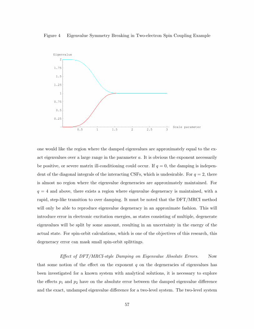
Figure 4 Eigenvalue Symmetry Breaking in Two-electron Spin Coupling Example
0.5 1 1.5 2 2.5 3Scale parameter
0.25
0.5
0.75
1
1.25
1.5
1.75
2
Eigenvalue
one would like the region where the damped eigenvalues are approximately equal to the ex-
act eigenvalues over a large range in the parameter a. It is obvious the exponent necessarily
be positive, or severe matrix ill-conditioning could occur. If q = 0, the damping is indepen-
dent of the diagonal integrals of the interacting CSFs, which is undesirable. For q = 2, there
is almost no region where the eigenvalue degeneracies are approximately maintained. For
q = 4 and above, there exists a region where eigenvalue degeneracy is maintained, with a
rapid, step-like transition to over damping. It must be noted that the DFT/MRCI method
will only be able to reproduce eigenvalue degeneracy in an approximate fashion. This will
introduce error in electronic excitation energies, as states consisting of multiple, degenerate
eigenvalues will be split by some amount, resulting in an uncertainty in the energy of the
actual state. For spin-orbit calculations, which is one of the objectives of this research, this
degeneracy error can mask small spin-orbit splittings.
Effect of DFT/MRCI-style Damping on Eigenvalue Absolute Errors. Now
that some notion of the effect on the exponent q on the degeneracies of eigenvalues has
been investigated for a known system with analytical solutions, it is necessary to explore
the effects p1 and p2 have on the absolute error between the damped eigenvalue difference
and the exact, undamped eigenvalue difference for a two-level system. The two-level system
57
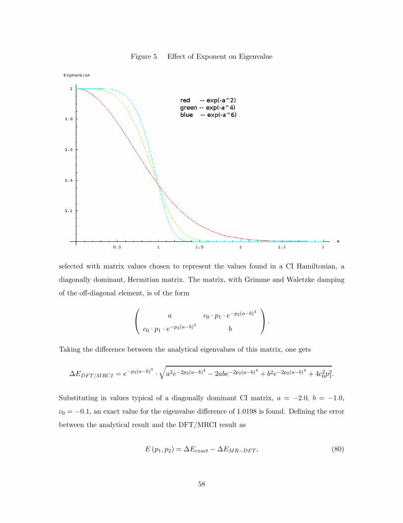
Figure 5 Effect of Exponent on Eigenvalue
selected with matrix values chosen to represent the values found in a CI Hamiltonian, a
diagonally dominant, Hermitian matrix. The matrix, with Grimme and Waletzke damping
of the off-diagonal element, is of the form
a c0 · p1 · e−p2(a−b)4
c0 · p1 · e−p2(a−b)4 b
.
Taking the difference between the analytical eigenvalues of this matrix, one gets
∆EDFT/MRCI = e−p2(a−b)4 ·√
a2e−2p2(a−b)4 − 2abe−2p2(a−b)4 + b2e−2p2(a−b)4 + 4c20p21.
Substituting in values typical of a diagonally dominant CI matrix, a = −2.0, b = −1.0,
c0 = −0.1, an exact value for the eigenvalue difference of 1.0198 is found. Defining the error
between the analytical result and the DFT/MRCI result as
E (p1, p2) = ∆Eexact − ∆EMR−DFT , (80)
58
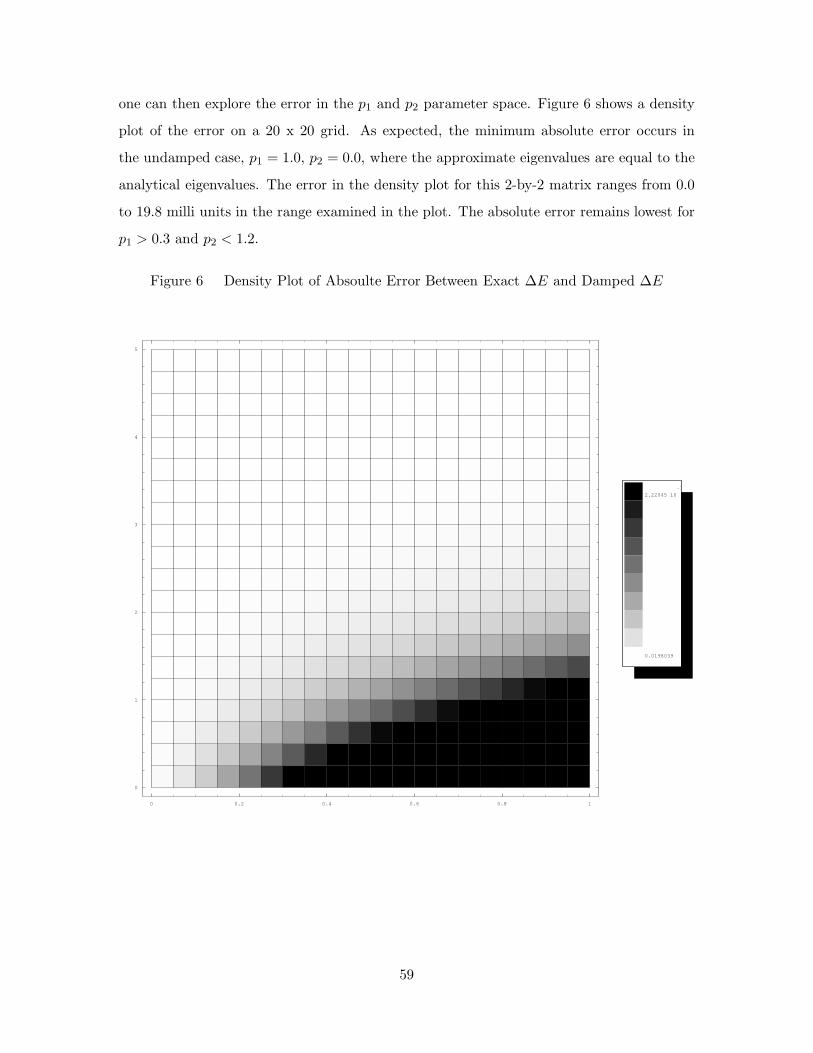
one can then explore the error in the p1 and p2 parameter space. Figure 6 shows a density
plot of the error on a 20 x 20 grid. As expected, the minimum absolute error occurs in
the undamped case, p1 = 1.0, p2 = 0.0, where the approximate eigenvalues are equal to the
analytical eigenvalues. The error in the density plot for this 2-by-2 matrix ranges from 0.0
to 19.8 milli units in the range examined in the plot. The absolute error remains lowest for
p1 > 0.3 and p2 < 1.2.
Figure 6 Density Plot of Absoulte Error Between Exact ∆E and Damped ∆E
0 0.2 0.4 0.6 0.8 1
0
1
2
3
4
5
0.0198039
-16
2.22045 10
59
DFT/MRCI Model Implementation with COLUMBUS
This chapter will describe the theory, development, testing, and validation of the the
Multi-reference Density Functional Theory (MR-DFT) method within COLUMBUS, modified
from the original model developed by Grimme and Waletzke (63). For reference, the various
program steps involved in performing a CI calculation in COLUMBUS are
1. Compute atomic orbital integrals using ARGOS
2. Perform ROHF SCF calculation to obtain molecular orbitals using SCFPQ
3. Generate the distinct row table for the specified CI expansion using CIDRT
4. Transform the atomic orbit integrals into molecular orbital integrals using TRAN
5. Sort the molecular orbital integrals into their various loop contributions (all-internal
through four-external plus spin-orbit integrals) and compute repartitioned Hamilto-
nian core energy with CISRT
6. Perform the MR-SOCISD calculation using CIUDG
Density Functional Theory Interface to COLUMBUS. The similarity between the
basic structure of Kohn-Sham self-consistent density functional theory and the HF codes
was pointed out earlier in this chapter. This similarity is one reason for the success of DFT,
in that many of the computational algorithms designed for HF calculations could be reused.
COLUMBUS contains an ROHF code, SCFPQ, but no DFT capability.
The best approach would be to implement a fully self-consistent numerical integration
scheme within SCFPQ. In this way, correlation potential integrals, which are used in the
construction of the Kohn-Sham effective Fock matrix, and correlation energy, which are
used to obtain the total DFT energy, are obtained from the one- and two-electron densities
at each iteration. However, implementing, validating, and testing a new numerical matrix
element evaluation scheme was simply not possible within the time available.
Instead, a different approach was taken, consisting of designing and implementing
an interface between another well-documented, validated, and tested DFT code, allowing
the use of the DFT specific elements in the Fock matrix in the ROHF code SCFPQ within
60
COLUMBUS, as well as in the molecular integral sorting program CISRT, so that the CIUDG
code could proceed using Kohn-Sham molecular orbitals and the correlation energy.
The basic elements that must be included in this interface between programs were
the one-electron correlation integrals, Vc and the correlation energies, Ec. The correlation
potential integral matrix elements are obtained by numerically integrating the functional
derivative of the correlation functional with respect to the density,
V cij =
⟨
ϕi
∣
∣
∣
∣
δFc [ρ]
δρ
∣
∣
∣
∣
ϕj
⟩
, (81)
where ϕi are atomic orbital basis functions. The correlation energy is obtained by numerical
integration of the correlation density functional over all space,
Ec =
∫
Fc [ρ] dτ. (82)
In order to obtain the correct Kohn-Sham molecular orbital coefficients, V xcij must be in-
cluded in the one-electron effective Fock matrix during the self-consistent iterations. Once
self-consistency is achieved, and the total DFT energy is computed, the correlation poten-
tial integrals are removed from the one-electron Fock matrix, and the correlation energy is
added. Failure to do this would yield the incorrect total energy. The one-electron contribu-
tion to the total Hartree-Fock energy is computed from the expression (127:176)
EHF1 =
1
2
∑
µ
∑
ν
PµνHcoreµν , (83)
with
Hcoreµν =
⟨
µ
∣
∣
∣
∣
∣
−1
2
N∑
i=1
∇2 −N∑
i=1
M∑
a=1
Za
ria
∣
∣
∣
∣
∣
ν
⟩
. (84)
The one-electron charge density matrix, Pµν is given by (127:139)
Pµν = 2
N2∑
a
CµaC∗νa, (85)
61

where Cµa are the basis contraction coefficients. However, in Kohn-Sham DFT, Hcoreµν is
given by
Hcoreµν =
⟨
µ
∣
∣
∣
∣
∣
−1
2
N∑
i=1
∇2 −N∑
i=1
M∑
a=1
Za
ria+ V c
µν
∣
∣
∣
∣
∣
ν
⟩
, (86)
while the total DFT energy is given by
EKS1 =
1
2
∑
µ
∑
ν
Pµν
(
Hcoreµν − V c
µν
)
+ Ec, (87)
with Ec defined in Equation 82. The main difference between the Hartree-Fock and Kohn-
Sham energies is that the Kohn-Sham total DFT energy is not obtained by contracting
the density matrix with the correlation potential integrals, but through integration of the
correlation density functional over all space. Thus, by extracting the correlation potential
integrals and correlation energy from a converged Kohn-Sham DFT calculation, one can
reproduce the density functional theory calculation in a Hartree-Fock program.
The first part of the interface required the extraction of the correlation potential
integrals and energies from NWChem. This was achieved by slightly modifying the xc getv.F
code, located in the \src\nwdft\xc directory in version 4.7. The correlation potentials and
energy are extracted from the calculation by setting the following variables
set "dft:idecomp" 2
anywhere in the NWChem input file, outside of any specific blocks. This forced NWChem to
separately compute the exchange energy and the correlation energy in a NWChem calculation,
rather than combine the two energies in a single value. Next, within the DFT block, the
following keywords enable the creation of the xcints file:
dft
print high
print "xc matrix"
end.
The code modifications to xc getv.F are placed after the numerical integration of the
density functional is performed in the call to subroutine grid quadv0, at line 332. The
modified code is
62
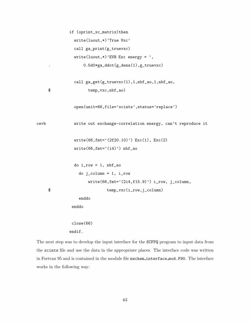
if (oprint_xc_matrix)then
write(luout,*)’True Vxc’
call ga_print(g_truevxc)
write(luout,*)’EVB Exc energy = ’,
. 0.5d0*ga_ddot(g_dens(1),g_truevxc)
call ga_get(g_truevxc(1),1,nbf_ao,1,nbf_ao,
$ temp_vxc,nbf_ao)
open(unit=66,file=’xcints’,status=’replace’)
cevb write out exchange-correlation energy, can’t reproduce it
write(66,fmt=’(2f20.10)’) Exc(1), Exc(2)
write(66,fmt=’(i4)’) nbf_ao
do i_row = 1, nbf_ao
do j_column = 1, i_row
write(66,fmt=’(2i4,f15.9)’) i_row, j_column,
$ temp_vxc(i_row,j_column)
enddo
enddo
close(66)
endif.
The next step was to develop the input interface for the SCFPQ program to input data from
the xcints file and use the data in the appropriate places. The interface code was written
in Fortran 95 and is contained in the module file nwchem interface mod.F90. The interface
works in the following way:
63

1. The COLUMBUS SCFPQ code must be compiled with the preprocessor definitions
-DEVB MULTIREFERENCE DFT and -D90 activated.
2. If the xcints file is not present, the SCFPQ code defaults to ROHF default behavior.
3. Before the first iteration of the SCF cycle, if the xcints file is present, it is opened,
and the contents, Ex, Ec, and V xcij are read into memory.
4. V cij are added to the one-electron Fock matrix, Hcore
ij for use in the SCF iterations.
The potentials are not included when the SCF energy is computed. Ec is added to
the total energy instead.
The design of this file-based interface was written to be general enough to facilitate the
introduction of any set of one-electron potentials to the Fock matrix. This could facilitate
further extensions to the SCFPQ code, for example, in adding a simple solvation model.
There is a potential for mismatch between SCFPQ and NWChem when using this file-based
interface, especially in open-shell atomic and molecular systems. For closed-shell systems,
NWChem uses a restricted Kohn-Sham algorithm, which interfaces nearly seamlessly into the
restricted Hartree-Fock algorithm used in SCFPQ. For open-shell systems, however, SCFPQ
uses a ROHF algorithm, while NWChem uses an unrestricted Kohn-Sham algorithm. In the
unrestricted case, the α and β orbitals are no longer constrained to remain degenerate, as is
the case in the restricted and restricted-open algorithms. The correlation potential integrals
may still be used in the file-based interface method, due to the fact that the correlation po-
tential integral matrix are integrals over basis functions, not molecular orbitals. However,
the resulting molecular orbital energies, coefficients, and the total energy obtained from the
unrestricted Kohn-Sham calculation and the modified ROHF method will necessarily differ.
In most cases examined, the discrepancy in the total DFT energy was small. This dis-
crepancy could be eliminated by implementing an in situ correlation numerical integration
capability with SCFPQ.
Another mismatch is in the normalization of the atomic orbital integrals in the NWChem
and SCFPQ programs. NWChem normalizes atomic orbital integrals to unity, while ARGOS, the
one- and two-electron integral program in the COLUMBUS program normalizes atomic orbitals
to a value dependent on the angular momentum value of the shell the atomic orbital is in.
64

For example, for a Gaussian orbital of the form
xmynzle−αr2
, (88)
where the orbital angular momentum, L for the atomic orbital is given by m+n+ l, then the
COLUMBUS atomic orbital normalization factor is (2m−1)!!(2n−1)!!(2l−1)!!. The (...)!! is the
odd factorial, defined by (2m − 1)!! = (2m − 1)(2m − 2)...(1). This normalization ensures
that orbitals in the same shell have the same normalization, and is identical to NWChem
normalization for shells with angular momentum L < 2. A normalization conversion had to
be incorporated into SCFPQ to ensure that the correlation potential integral normalization
was consistent. This was accomplished by multiplying the NWChem correlation potential
integrals by the COLUMBUS normalization factor.
Although both programs can exploit Abelian point group symmetry, each program
approaches symmetry in a slightly different fashion. NWChem uses a projection operator
approach, projecting out the various irreducible representations from the state vector. On
the other hand, SCFPQ explicitly works in a symmetry-adapted atomic orbital basis. In his
basis, the Fock matrix is block diagonal, and there is no symmetry contamination in the
state vector. Developing a one-to-one interface between the two programs that incorporated
point group symmetry as well proved to be too complicated to accomplish in the scope of
this research. As a result, all interface calculations must be performed in the C1 Abelian
point group at this time.
DFT Interface Validation. Table 10 lists the total DFT energies produced
from both NWChem and the modified version of SCFPQ for atomic and diatomic systems over
a range of ground state multiplicities. The doublet and triplet systems are open-shell atoms,
and are calculated using an unrestricted Kohn-Sham DFT treatment in NWChem, but with
the modified ROHF method described above in SCFPQ.
Open-shell atomic cases were calculated in SCFPQ using a set of high-spin open-shell
coefficients, but with the correlation potential integrals and energy from an unrestricted
Kohn-Sham DFT calculation. As expected, this mismatch introduces a slight discrepancy
into the DFT energy produced by SCFPQ. The discrepancy between the NWChem and SCFPQ
65
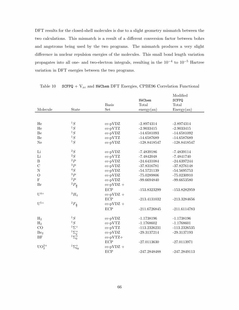
DFT results for the closed-shell molecules is due to a slight geometry mismatch between the
two calculations. This mismatch is a result of a different conversion factor between bohrs
and angstroms being used by the two programs. The mismatch produces a very slight
difference in nuclear repulsion energies of the molecules. This small bond length variation
propagates into all one- and two-electron integrals, resulting in the 10−4 to 10−5 Hartree
variation in DFT energies between the two programs.
Table 10 SCFPQ + Vxc and NWChem DFT Energies, CPBE96 Correlation Functional
ModifiedNWChem SCFPQ
Basis Total TotalMolecule State Set energy(au) Energy(au)
He 1S cc-pVDZ -2.8974314 -2.8974314He 1S cc-pVTZ -2.9033415 -2.9033415Be 1S cc-pVDZ -14.6581093 -14.6581092Be 1S cc-pVTZ -14.6587689 -14.6587689Ne 1S cc-pVDZ -128.8418547 -128.8418547
Li 2S cc-pVDZ -7.4839186 -7.4839114Li 2S cc-pVTZ -7.4842048 -7.4841740B 2P cc-pVDZ -24.6431084 -24.6397244C 3P cc-pVDZ -37.8316781 -37.8276148N 4S cc-pVDZ -54.5721139 -54.5695753O 3P cc-pVDZ -75.0289806 -75.0230910F 2P cc-pVDZ -99.6694840 -99.6653580Br 2P 3
2
cc-pVDZ +
ECP -153.8323299 -153.8282959U4+ 3H4 cc-pVDZ +
ECP -213.4131032 -213.3284656U5+ 2F 5
2
cc-pVDZ +
ECP -211.6726845 -211.6114783
H21S cc-pVDZ -1.1738196 -1.1738196
H21S cc-pVTZ -1.1768602 -1.1768601
CO 1Σ+ cc-pVTZ -113.2326231 -113.2326535Be2
1Σ+g cc-pVDZ -29.3137214 -29.3137193
BF 1Σ+
0 cc-pVTZ+ECP -27.0113630 -27.0113971
UO2+
21Σ+
0g cc-pVDZ +
ECP -247.2848488 -247.2849113
66

Correlation Energy in the Repartitioned Hamiltonian. Once a set of pseudo-Kohn-
Sham orbitals is generated through the file-based interface between NWChem and SCFPQ,
the distinct row table for the CI calculation is generated using the CIDRT program, and
the integrals over atomic orbitals are transformed into a molecular orbital basis using the
TRAN program. The only step remaining before actually performing the CI calculation is
to sort the molecular integrals into all-internal, one-external, two-external, three-external,
and four-external orbital index sets and compute the reference energy of the repartitioned
Hamiltionian. This sorting is accomplished by the CISRT program.
The critical component in an DFT/MRCI calculation is the addition of the correlation
energy needs to the reference energy. This is accomplished through the file-based interface,
xcints. In a similar fashion to the modified ROHF program, the modified CISRT program
performs the following:
1. The COLUMBUS CISRT code must be compiled with the preprocessor definitions
-DEVB MULTIREFERENCE DFT and -D90.
2. If the xcints file is not present, the CISRT code defaults to its default behavior.
3. If the xcints file is present, it is opened, and the contents, Ex, Ec are read into
memory.
4. Ec is added to the reference energy of the repartitioned Hamiltonian.
This final step adds the correlation energy to the reference energy, effectively offset-
ting the energies produced in the CIUDG program by Ec. For a single root, ground state
calculation, with zero excitations from the reference space, this reproduces the DFT energy
result obtained in the modified SCFPQ program exactly. A more ideal approach would be to
recompute the correlation energy contribution based on the orbital density for each refer-
ence. This approach would allow a more reasonable approximation to the correlation energy
for each reference, rather than use the correlation energy obtained from the ground state
density and applied to all reference configurations, which may give rise to vastly different
densities.
67
CIUDG Based DFT/MRCI. The third and final step in the implementation of the
DFT/MRCI method required modification of the CI program, CIUDG, in order to implement
the damping of the off-diagonal CI matrix elements.
Modifications to the Grimme and Waletzke DFT/MRCI Model. In their
paper (63), Grimme and Waletzke describe an approach to the development of a hybrid
DFT-CISD model. Their approach, based on a selected-CI code, involved modification of
both the diagonal and off-diagonal CI Hamiltonian matrix elements. The fact that they
used a selected-CI code enabled them to select which CSFs to include in their CI expansion.
The DFT/MRCI model and their CSF selection criteria allowed them to drastically reduce
the size of the CI expansions necessary to examine systems of interest. The rationale behind
this is the fact that the DFT calculation captures a large fraction of the dynamic correlation
energy, and so only a modest CI expansion is necessary to model the non-dynamic correlation
contribution to the energy.
The approach they described in their paper involved a hybrid correlation functional,
half exact HF exchange and half Becke 1988 (11) exchange functional, coupled with the
Lee, Yang, and Parr (81) GGA correlation functional. Their resulting DFT/MRCI model
contained five unknown parameters, shown in chapter two, equations 75, 76, and 77.
In this model, however, only the off diagonal matrix element damping was retained.
The rationale behind this was that modifications to the diagonal CI matrix elements were
necessary due to the use of an approximate, local exchange functional. Using a correlation-
only functional and eliminating the modifications to the diagonal matrix elements reduced
the number of empirical damping parameters to two. However, using the exact Hartree-
Fock exchange operator with Kohn-Sham orbitals does not reproduce the exact exchange
energy. Most successful hybrid density functionals mix exact Hartree-Fock exchange for the
non-local contribution with a portion of local exchange energy obtained from the exchange
functional. Perdew and Ernzerhof suggest a rationale for mixing 15% to 30% exact Hartree-
Fock exchange with 70% to 85% local density functional approximation (102). Grimme
and Waletzke use the BHLYP density functional approximation, which mixes 50% exact
exchange with 50% Becke exchange density functional approximation. A popular and accu-
rate hybrid density functional, Becke Three Parameter Hybrid Density Functional (B3LYP)
68
mixes 20% Hartree-Fock exchange with 72% Becke exchange. Using a correlation only func-
tional and 100% exact Hartree-Fock exchange simplifies the treatment of the diagonal CI
matrix elements, and allows a more flexible treatment of various spin multiplicities, without
resorting to additional parameterization of the method, in exchange for some error in the
exchange energy contribution.
Full advantage was taken of the loop-driven approach in CIUDG in implementing the
damping of the off-diagonal matrix elements. By taking care to identify the individual
CSFs participating in a particular one- or two-body loop interaction within Configuration
Interaction Unitary Diagonalize (CIUDG), and applying the scaling appropriately based on
Equation 77, the overall scaling factor for each off-diagonal element can be constructed in a
factored form. In the GUGA approach to CI calculations, the various contributions to the
CI Hamiltonian are constructed from the product of individual segment values within the
loop (120:73) (124).
Off-diagonal matrix element scaling is introduced through a scaling factor, ρ (i, j)
applied to both one- and two-body segments, defined by
ρ (i, j) = p1e−p2∆E4
ij , (89)
where ∆Eij is the diagonal integral difference between CSF i and CSF j. This results in
new one- and two body generator matrix elements,
⟨
m′ |Eij |m⟩
=∏
k=(i,j)
ρ (i, j)ω(
Qk; d′kdk,∆bk, bk
)
(90)
and⟨
m′ |eij,kl|m⟩
=∏
p∈S1
ρ (i, j)ω (Tp, bp)∑
x=0,1
∏
p∈S2
ωx (Tp, bp) . (91)
CIUDG based DFT/MRCI Model Validation. The critical step in implementing
the method was to correctly identify the interacting CSFs in each loop contribution. One
of the efficiencies of the loop-driven approach to CI calculations in the GUGA approach is a
result of the compact nature of the DRT. Large CI expansions can be compactly described
with compact DRT tables without having to form and store an index vector of the same
69
dimension as the CI expansion. Such compactness is desirable in very large CI expansions,
as forming and storing an index vector of millions, or billions of elements long is highly
inefficient.
The loop-driven approach indexes loop contributions to internal walks, which are all
the walks through the DRT of the occupied reference space. The regular structure of the
external space (see Figure 1) is exploited for code efficiency. These internal walks terminate
at the beginning of the external space on either Z, Y, X, or W vertices. The CIUDG code is
organized according to the types of loop contributions, based on the excitation level with
respect to the internal space. A maximum of two orbitals can contribute to one-body loop
types, while a maximum of four orbitals can contribute to two-body loops. Calculations
proceed in order, computing the following loop type contributions to the CI Hamiltonian:
1. Four-external loops – All four orbitals contributing to this loop are in the external
(virtual orbital) space. The structure of these matrix element contributions to the
CI Hamiltonian can be either a single matrix element, a row or column of matrix
elements, or a m x m block of matrix elements. There are 16 separate locations in the
code that perform this type of interaction, based upon the symmetry of the bra and
ket CSFs.
2. Three-external loops – One orbital is in the internal space, three orbitals are in
the external space. The structure of these matrix element contributions to the CI
Hamiltonian can be either a row or column of matrix elements, or a m x m block of
matrix elements. There are 9 separate types of this interaction in the code.
3. Two-external loops – Two orbitals are in the internal space, two orbitals are in the
external space. The vast majority of these matrix element contributions to the CI
Hamiltonian are in the form of m x m block of matrix elements, with only one row
or column vector contribution. There are 20 separate types of this interaction in the
code.
4. One-external loops – Three orbitals are in the internal space, and one orbital is in
the external space. All these contributions are either row or column vectors in the CI
Hamiltonian. There are 6 types of this loop interaction in the code.
70
5. All-internal loops – All four orbitals in the interaction are in the internal space.
There are 4 types of this loop interaction in the code, with the contributions appearing
as either a single CI matrix element, or a co-diagonal vector.
6. Spin-orbit integral loops – Since the spin-orbit operator is a one-body operator,
there can only be two- and one-external loop types of this, in addition to all-internal
spin orbit loops. These interactions were not modified in this implementation.
For each loop type, the CSFs involved was based upon the sum of the CSF offset for
each internal walk and the CSF offset for the number of CSFs involved in the interaction.
Each loop contribution eventually ends with a Basic Linear Algebra System (BLAS) sub-
routine call to update the sigma vector from the CI vector. This update is usually of the
form
~σ = H · ~c. (92)
The CSFs involved in the update were identified through the CSFs involved in both the ~σ
vector and ~c vector, as the Hamiltonian, H is never explicitly constructed. In the CIUDG
code, both the sigma and CI vectors are indirectly indexed, with locations in the vectors
defined and controlled as offsets to the starting CSF for the internal walks in the interaction.
The internal walks are organized according to the Z, Y, X, or W walk vertex upon which
they terminate. Z and Y walks are listed first, so Z walks always begin at CSF number 1.
The starting CSFs of the Y, X, and W walks are also stored, but only for the internal walks.
So the starting CSFs for the sigma and CI vectors in an all-internal interaction between
two Y walks would occur at the internal Y walk start CSF. The range of CSFs involved
in the interaction is then deduced by the type of BLAS subroutine call. In the YY walk
all-internal interaction example, the sigma vector update is performed by the pair of BLAS
subroutine calls
call daxpy(ny,hint,ciket(nmb2+1),1,sigmabra(nmb1+1),1)
call daxpy(ny,hint,cibra(nmb1+1),1,sigmaket(nmb2+1),1).
All sigma vectors get updated in this pairwise fashion, which takes advantage of the
Hermitian nature of the CI Hamiltonian to update the sigma vector in two places, one
71

update due to the lower triangle of the CI Hamiltonian, the other due to the contribution
from the upper triangle of the Hamiltonian. In the YY interaction example, the daxpy
subroutine call performs the following operation:
~y = a ∗ ~x+ ~y, (93)
where a is a scalar, ~x and ~y are both vectors. In the code segment above, the dimension
of these vectors are ny and the offsets to the internal Y walk starting CSFs for each are
nmb2+1 and nmb1+1. The scalar a is hint. In this example, hint is the CI Hamiltonian
matrix element, and the shape of this interaction in the Hamiltonian is a co-diagonal vector.
Unrolling this loop so that off-diagonal matrix element scaling can occur, along with the
update of the sigma vector is performed by the following code,
hint_original = hint
do temp=1, ny
call scale_scalar(cist(2)+nmb1+temp, &
cist(1)+nmb2+temp, hint)
sigmabra(nmb1+temp)=sigmabra(nmb1+temp)+&
hint*ciket(nmb2+temp)
sigmaket(nmb2+temp)=sigmaket(nmb2+temp)+&
hint*cibra(nmb1+temp)
hint = hint_original
end do.
Hence, the indices of the Hamiltonian matrix element referred to in the code by hint
is given by the sum of the Y walk starting CSF in both the CI vector and the sigma vector,
72
and the offset from these starting CSFs. For the CI vector, this sum is cist(1)+nmb2+temp
while for the sigma vector, the sum is cist(2)+nmb1+temp.
Careful analysis along these lines of all the loop BLAS calls allowed reconstruction of
the absolute CSFs involved in each interaction from the various offsets.
From the BLAS routines used to update the sigma vector, the possible types of CI
matrix elements are:
1. Scalar – A single CI matrix element contributes to the ~σ update.
2. Vector – Either a row or column of matrix elements contribute to the ~σ update. These
vectors are either n x 1 or 1 x m in size.
3. Block – An n x n block of matrix elements contributes to the ~σ update.
Three separate scaling routines were written to account for each case listed above.
For the block matrices and vectors, there were several locations in the CIUDG code
where significant optimization of the ~σ vector update occurs. In these areas, it was not
possible to identify what the CSF locations of the matrix elements were in general expansion.
These cases occur in the CIUDG code where the CI vector gets either symmetrically or
asymmetrically expanded into an n x n matrix. In these cases, the update of the sigma
vector no longer takes the form of Equation 92. Instead, the sigma vector gets updated
in a complicated matrix/matrix product fashion. For these loop types, involving a small
number of external orbitals, with one, two, or three external basis functions, the optimization
could be unrolled, and the sigma update reformulated in terms of a matrix/vector product,
where identification of the CSFs is then possible. However, no general pattern arose in the
assignment of CSFs to matrix elements.
Because of this non-unique usage of the two-electron molecular integrals in the update
of the σ vector, the implementation of the Grimme and Waletzke DFT/MRCI approach
required slight modification in the GUGA based CI code . In these cases, which arise in
two of the six one-external loops, and six of the twenty two-external loop types, a different
approach was taken. For these blocks of matrix elements, if the dimension of the block is
greater than one, a single scaling factor is applied to the entire block of matrix elements.
Three scaling choices are possible, and they are selectable in the input file via a logical
73
flag: minimum scaling, maximum scaling, or average scaling. In these cases, the ranges
of CSFs in the block can be deduced in general, however, the matrix elements within the
block are not uniquely used, which precludes damping them individually. Instead, based
on the CSF range, and the flag chosen in the input file, the entire block of matrix elements
gets damped by the same factor. This is a more efficient method for damping these highly
optimized cases, and is necessary for two reasons. First, in these blocks, matrix elements
are not used uniquely in the block. The same integral contributes to more than one matrix
element, precluding individual, unique damping. Second, because of the optimization, linear
combinations of integrals contribute to the block, with each integral contribution within a
linear combination possibly having differing CSF indices. Block damping the entire group of
matrix elements by a single factor, by either the maximum, minimum, or average damping
factor based on the CSF range of the block was the way that code efficiency was preserved.
Additionally, it is simply not feasible to single out specific CSFs for inclusion in the
CI expansion in the loop-driven, GUGA-based CI code, CIUDG. However, reduction in the
size of the CI expansion is one of the most important factors in the Grimme and Waletzke
model. Rather than selectively include CSFs in the expansion, as Grimme and Waletzke
did using their CI code, expansion size in CIUDG is limited by freezing orbitals in the virtual
space, using the rationale that high energy virtual orbitals contribute very little to the
non-dynamic correlation energy.
Testing the DFT/MRCI Model Implementation within CIUDG. Using the fact that
the absolute CSFs of both the sigma and CI vectors involved in the interactions could be
reconstructed, an internal consistency check was coded into CIUDG. This check worked by
constructing the Hamiltonian from the loop contributions and their absolute CSFs. This
Hamiltonian was then diagonalized, and the eigenvalues were compared to the eigenvalues
obtained from the iterative Davidson diagonalization of the subspace matrix. Incorrect
indexing of the CSFs resulted in incorrectly placing the matrix element within the consis-
tency check Hamiltonian, and resulted in eigenvalues that did not agree with those obtained
iteratively from the subspace matrix.
The CI program never explicitly generates the Hamiltonian, instead, it generates so-
called matrix-vector products, H~v directly, where ~v are the reference vectors. The subspace
74
matrix is generated by forming the product ~vH~v. In the first iteration, the start vectors
are constructed by placing a 1 in the CSF location for that particular vector, with zeros
elsewhere. Starting vectors can be generated using Z walks, or Z and Y walks, defining the
set of reference vectors upon which to generate the subspace matrix. The subspace matrix
and CI Hamiltonian are equal in this case during the first iteration. As the starting vectors
converge in subsequent iterations, this is no longer true.
This behavior of the subspace matrix was exploited for testing purposes, and code
was added to generate start vectors for all Z, Y, W, and W walks (accessed by setting
ISTRT=3, IVMODE=1 in the ciudgin namelist input file). As explained above, this allowed
construction of a subspace matrix that corresponded to the exact CI Hamiltonian. This
exact Hamiltonian was used as a reference to aid in the determination of absolute CSF
locations.
A series of very small test systems were used to generate and test the determination
of absolute CSF assignments. By setting p1 = 1.0 and p2 = 0.0, the off-diagonal elements
were unaffected, and the consistency check Hamiltonian and the exact Hamiltonian could
be compared, facilitating debugging of the DFT/MRCI code. A series of systems with very
small basis sets were used to facilitate this, so that the entire CI Hamiltonian could be
visualized. The atomic systems used to perform this testing, along with their basis sets and
point group symmetry are listed in Table 11.
75
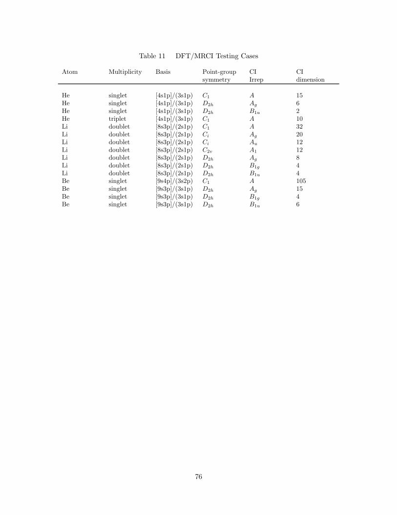
Table 11 DFT/MRCI Testing Cases
Atom Multiplicity Basis Point-group CI CIsymmetry Irrep dimension
He singlet [4s1p]/(3s1p) C1 A 15He singlet [4s1p]/(3s1p) D2h Ag 6He singlet [4s1p]/(3s1p) D2h B1u 2He triplet [4s1p]/(3s1p) C1 A 10Li doublet [8s3p]/(2s1p) C1 A 32Li doublet [8s3p]/(2s1p) Ci Ag 20Li doublet [8s3p]/(2s1p) Ci Au 12Li doublet [8s3p]/(2s1p) C2v A1 12Li doublet [8s3p]/(2s1p) D2h Ag 8Li doublet [8s3p]/(2s1p) D2h B1g 4Li doublet [8s3p]/(2s1p) D2h B1u 4Be singlet [9s4p]/(3s2p) C1 A 105Be singlet [9s3p]/(3s1p) D2h Ag 15Be singlet [9s3p]/(3s1p) D2h B1g 4Be singlet [9s3p]/(3s1p) D2h B1u 6
76
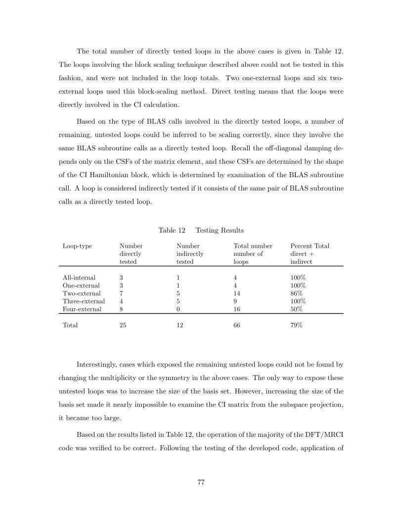
The total number of directly tested loops in the above cases is given in Table 12.
The loops involving the block scaling technique described above could not be tested in this
fashion, and were not included in the loop totals. Two one-external loops and six two-
external loops used this block-scaling method. Direct testing means that the loops were
directly involved in the CI calculation.
Based on the type of BLAS calls involved in the directly tested loops, a number of
remaining, untested loops could be inferred to be scaling correctly, since they involve the
same BLAS subroutine calls as a directly tested loop. Recall the off-diagonal damping de-
pends only on the CSFs of the matrix element, and these CSFs are determined by the shape
of the CI Hamiltonian block, which is determined by examination of the BLAS subroutine
call. A loop is considered indirectly tested if it consists of the same pair of BLAS subroutine
calls as a directly tested loop.
Table 12 Testing Results
Loop-type Number Number Total number Percent Totaldirectly indirectly number of direct +tested tested loops indirect
All-internal 3 1 4 100%One-external 3 1 4 100%Two-external 7 5 14 86%Three-external 4 5 9 100%Four-external 8 0 16 50%
Total 25 12 66 79%
Interestingly, cases which exposed the remaining untested loops could not be found by
changing the multiplicity or the symmetry in the above cases. The only way to expose these
untested loops was to increase the size of the basis set. However, increasing the size of the
basis set made it nearly impossible to examine the CI matrix from the subspace projection,
it became too large.
Based on the results listed in Table 12, the operation of the majority of the DFT/MRCI
code was verified to be correct. Following the testing of the developed code, application of
77
the DFT/MRCI model to various atomic and molecular systems to assess the performance
could commence.
Using the COLUMBUS DFT/MRCI Model
DFT/MRCI Model Input Control. Input to the COLUMBUS-based DFT/MRCI
model is contained in the input to the CIUDG program. Activation of the DFT/MRCI code
and control of its various features is accomplished by a series of flags, added to the name
list input file for CIUDG, ciudgin. The default behavior of the CIUDG code is to not perform
DFT/MRCI calculations. DFT/MRCI capability has to be specifically activated in order
to perform a DFT/MRCI calculation. As in was the case with the modified SCFPQ and
CISRT programs, in order to perform a DFT/MRCI calculation, the CIUDG program must
be compiled with the preprocessor definitions -DEVB MULTIREFERENCE DFT and -D90. The
following input flags, along with example values, are possible in the ciudgin file to control
the behavior of the DFT/MRCI code:
p1 = 0.96
p2 = 2.5
scale_power = 4
od_allint_damp = .t.
od_1ext_damp = .t.
od_2ext_damp = .t.
od_3ext_damp = .t.
od_4ext_damp = .t.
coarse_scaling = ’minimum’
dump_diag = .f.
debug_file = .f.
loop_track = .f.
The first three input flags, control the off-diagonal damping of the CI matrix elements. The
scale_power flag sets the exponent on the ∆E term in Equation 77. The four od_*_damp
flags activate the damping of the various loop contributions. Each individual loop type
(all-internal, one-external, etc.) can be selectively damped. The next flag, coarse_scaling
78
controls the block scaling in the eight optimized loop interactions discussed earlier. Three
choices exist for this flag: ’minimum’, which scales the entire block by the minimum damping
factor, ’average’, which damps the entire block of loop interactions by the average damping
factor for the entire block, and ’maximum’, which applies the largest damping factor in
the block to the entire block of matrix elements. The final three flags are for debugging.
Diagonal CSF integrals can be dumped to a human readable file by setting dump_diag,
while debug_file controls dumping of verbose information about the off-diagonal scaling
to a human readable text file, and loop_track identifies which loop types, as indexed by
an arbitrary numeric label, are being accessed in a calculation.
Usage. The procedure for using the COLUMBUS-based DFT/MRCI model is
listed below. Before proceeding, a version of NWChem with the modifications listed earlier
must be compiled in order to extract Vc and Ec from a DFT calculation. A version of
COLUMBUS with the DFT/MRCI model needs to be compiled with the preprocessor flags
described earlier enabled. The procedure below describes how to use the DFT/MRCI model
using a DFT correlation functional and 100% HF exchange. This implementation of the
DFT/MRCI model can not be used with a hybrid density functional. Using a mixture
of HF and approximate density functional exchange, in the implementation described by
Grimme and Waletzke, requires additional modifications to the diagonal matrix elements,
which introduce spin-multiplicity limitations to the model.
The first thing that needs to be done is to determine useful values for the two free
parameters in the damping term, Equation 78. Appendix B lists the atomic and molecular
systems used to determine the two free damping parameters p1 and p2 in Equation 78, for
this research. A generic procedure for determining the damping parameters is:
1. Perform FCI calculation on the atomic or molecular system used in the training set.
Compute both the ground state and at least one excited state of the same multiplicity.
Be sure to use C1 point group symmetry. GAMESS (95) (98) was used in this research
to perform the FCI calculations.
2. Using 100% HF exchange and an approximate LDA, GGA, or meta-GGA correlation
functional, perform a DFT calculation on the atomic or molecular system used in the
79
training set in order to extract Ec and Vc. Be sure to use C1 point group symmetry.
The external files overlap and xcints are generated by keywords in the NWChem input
file described in a previous section.
3. Setting a particular value of p1 and p2 in the CIUDG input control specified in the next
section, run the following series of COLUMBUS programs (either individually, or via a
script):
(a) Generate the atomic orbital integrals using ARGOS. Take care to ensure that the
symmetry adapted linear combinations of atomic orbital matrices in the ARGOS
input file match the ordering used in NWChem. NWChem orders the various orbital
shells from lowest to highest ml value, while the symmetry-adapted linear com-
bination matrices generated automatically by either IARGOS or CIML arbitrarily
order the atomic orbitals.
(b) Run the SCFPQ program. Be sure the files xcints and overlap have been gen-
erated by NWChem. If performing an open-shell calculation, use the unrestricted
DFT option in NWChem, and use either the average of configurations or high-
spin open shell coefficients in SCFPQ. The average of configuration open-shell
coefficients, along with fractional occupation in open-shell SCFPQ calculations
better preserve the symmetry of orbitals within the same shell. NWChem does
not typically perform spherically averaged open-shell calculations in ROHF and
unrestricted DFT
(c) Check the total SCF energy from SCFPQ and NWChem to ensure the DFT ener-
gies are in agreement, especially for closed shell cases. Discrepancies here arise
typically from an inconsistency in the ordering of the atomic orbital basis in the
Fock matrix between the ARGOS and NWChem programs.
(d) Examine the orbital energies in the SCFPQ output. Determine an acceptable vir-
tual orbital cutoff point based on orbital energies. In this research, an acceptable
cutoff was found to range from 30 to 40 eV above the highest occupied molecular
orbital. Take care not to freeze orbitals in such a way that symmetry is broken.
For example, this can happen if only two of three p degenerate orbitals are frozen
in an atomic calculation.
80
(e) Generate the DRT using CIDRT, freezing virtual orbitals above the cutoff orbital
energy in order to limit the size of the CI expansion. This may require several
iterations to find a good balance between CI expansion size and DFT/MRCI
accuracy. In the GUGA direct CI method, loop contributions are formed di-
rectly from one- and two-electron integrals, bypassing explicit construction of
the Hamiltonian and CSFs. Limited selection of interacting CSFs can be ac-
complished in the GUGA approach either through removing specific levels in the
DRT, removing specific walks from the DRT, or by freezing virtual orbitals in
the external portion of the graph.
(f) Transform the atomic orbital integrals to molecular orbital integrals using TRAN.
(g) Sort the molecular integrals into internal, external and frozen orbitals and com-
pute the repartitioned Hamiltonian reference energy with CISRT. Ensure the file
xcints is present in order to incorporate the DFT Ec energy into the reference
energy.
(h) Specify the DFT/MRCI specific input in the CIUDG input file. At a minimum,
p1 and p2 must be specified. By default, coarse scaling is selected to be set
to .minimum.. This forces block scaling to be performed using the minimum
damping factor over the entire block of integrals. This was done in order to avoid
situations where overly large scaling gets applied to important loop contributions.
The drawback is the fact that some loop contributions may not be scaled enough
using this scheme.
4. Repeat the COLUMBUS steps above, changing p1 and p2. In this research, a script was
used to automatically vary the damping parameters, with p1 ranging from 0.0 to 1.0,
and p2 ranging from 0.0 to 10.0, both over 20 steps. The excitation energy between
the ground and excited state was computed at each value of p1 and p2, and dumped
to a file to facilitate the plotting and analysis contained in Appendix B.
5. Compute the difference between the FCI and DFT/MRCI excitation energies for each
pair of p1 and p2 values computed above.
6. Look for a region in the density plot (Figure 7) of absolute excitation energy error
between the FCI and DFT/MRCI that is a minimum, and where p1 and p2 decouple.
81
This fixes the value of p1. The value of p2 is selected from an asymptotically flat region
of absolute error along this value of p1. In this research, using 100% HF exchange
and the PBE 1996 GGA correlation functional, with a selection of training systems
spanning the first two rows of the periodic table, the damping parameters decoupled
at p1 = 0.96. The absolute error for all values of p2 > 2.0 was roughly constant for
p1 = 0.96. These considerations led to the selection of p1 = 0.96 and p2 = 2.5 for this
research using 100% HF exchange and PBE 1996 GGA correlation functional.
All DFT and TDDFT calculations were performed using the Perdew Burke and Ernz-
erhof pure correlation functional (CPBE96) correlation functional. Currently, NWChem can
not do TDDFT calculations using meta-GGA functionals, limiting this analysis to at most
GGA functionals. A small set of test atoms and molecules was selected and used to deter-
mine a set of damping parameters that produce acceptable error for all systems.
Error was defined as the difference between the DFT/MRCI excitation energy and
the FCI excitation energy for the same electronic transition. Both DFT/MRCI and FCI
calculations used the same basis set and/or effective core potential.
Appendix B lists the test atomic and molecular systems, the FCI calculations results,
and density plots for the absolute error for each systems used to determine the universal
damping parameters for the CPBE96 correlation functional. The test set consists of both
double- and triple-ζ quality basis sets for atoms and diatomics. Ground state spin multiplic-
ities ranges from singlet through quartet, and cover both closed- and open-shell systems,
with open s- and p-shells. The original method proposed by Grimme and Waletzke was
limited to singlet and triplet states. The spin-orbit extension to the original DFT/MRCI
method developed by Kleinschmidt et al also contained this spin-multiplicity limitation.
Figure 7 shows a density plot of this averaged data on the p1/p2 grid.
A clear band of minimum error exists in the density plot shown in Figure 7, ranging
over p1 values of roughly 0.8 to 0.96 and over p2 values from 0 through 10. The band
stabilizes and is essentially constant for values of p1 ≈ 0.96 and p2 > 2.0. The global
minimum averaged, normalized error occurred in the combined data at the values p1 = 0.85,
p2 = 0.5. The stabilization of the minimum error band seems to indicate an asymptotic
region where the damping parameters produce decent result across the range of test cases.
82
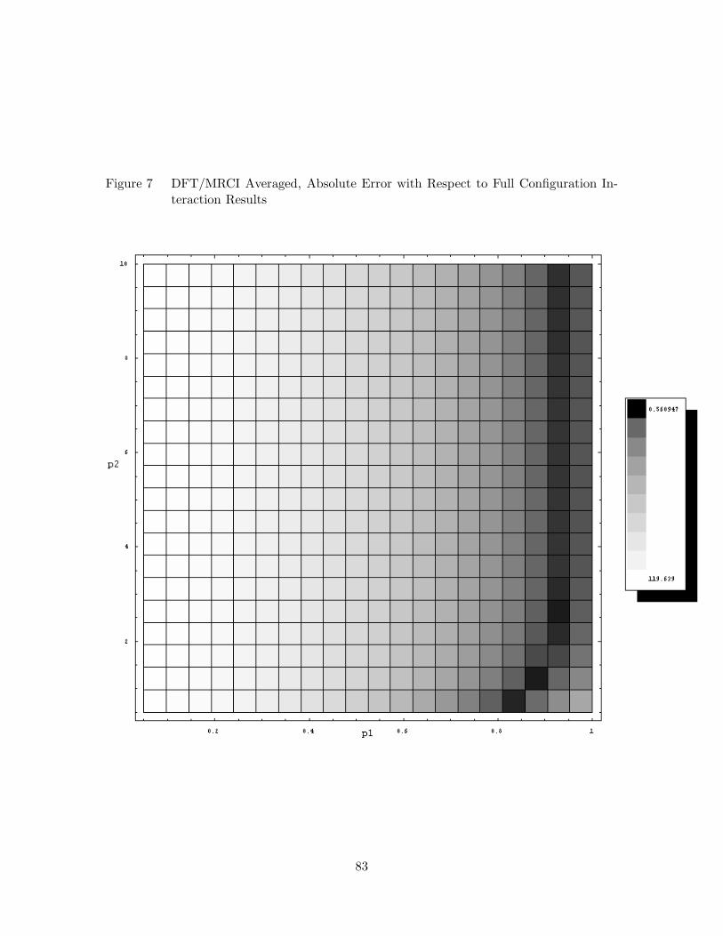
Figure 7 DFT/MRCI Averaged, Absolute Error with Respect to Full Configuration In-teraction Results
83
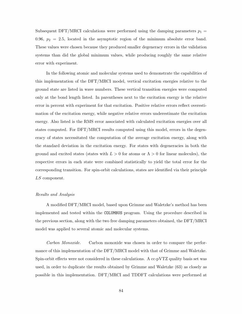
Subsequent DFT/MRCI calculations were performed using the damping parameters p1 =
0.96, p2 = 2.5, located in the asymptotic region of the minimum absolute error band.
These values were chosen because they produced smaller degeneracy errors in the validation
systems than did the global minimum values, while producing roughly the same relative
error with experiment.
In the following atomic and molecular systems used to demonstrate the capabilities of
this implementation of the DFT/MRCI model, vertical excitation energies relative to the
ground state are listed in wave numbers. These vertical transition energies were computed
only at the bond length listed. In parentheses next to the excitation energy is the relative
error in percent with experiment for that excitation. Positive relative errors reflect overesti-
mation of the excitation energy, while negative relative errors underestimate the excitation
energy. Also listed is the RMS error associated with calculated excitation energies over all
states computed. For DFT/MRCI results computed using this model, errors in the degen-
eracy of states necessitated the computation of the average excitation energy, along with
the standard deviation in the excitation energy. For states with degeneracies in both the
ground and excited states (states with L > 0 for atoms or Λ > 0 for linear molecules), the
respective errors in each state were combined statistically to yield the total error for the
corresponding transition. For spin-orbit calculations, states are identified via their principle
LS component.
Results and Analysis
A modified DFT/MRCI model, based upon Grimme and Waletzke’s method has been
implemented and tested within the COLUMBUS program. Using the procedure described in
the previous section, along with the two free damping parameters obtained, the DFT/MRCI
model was applied to several atomic and molecular systems.
Carbon Monoxide. Carbon monoxide was chosen in order to compare the perfor-
mance of this implementation of the DFT/MRCI model with that of Grimme and Waletzke.
Spin-orbit effects were not considered in these calculations. A cc-pVTZ quality basis set was
used, in order to duplicate the results obtained by Grimme and Waletzke (63) as closely as
possible in this implementation. DFT/MRCI and TDDFT calculations were performed at
84

a bond length 1.1261 A, obtained from the National Institute of Standards and Technology
(NIST) Computational Chemistry Comparison and Benchmark DataBase (CCCBDB) (1).
This bond length was generated from a DFT geometry optimization using a cc-pVTZ quality
basis set and the hybrid B3LYP GGA correlation density functional.
Table 13 lists the DFT/MRCI, TDDFT, and experimental results for the carbon
monoxide molecule. The first two σ orbitals, corresponding to the carbon and oxygen 1s
orbitals, were frozen, as were the 44 highest energy virtual orbitals. The Kohn-Sham orbital
energy difference between the Highest Occupied Molecular Orbital (HOMO) and the first
frozen virtual orbital was roughly 38 eV. All reference configurations from a Complete Active
Space (CAS) over the carbon and oxygen 2s and 2p orbitals was used in this calculation,
corresponding to 10 active electrons in 8 orbitals. The CI expansion sizes resulting from
this active space were 87,612 singlet CSFs and 145,620 triplet CSFs. Without freezing of
the high energy virtual orbitals, the singlet CI expansion size was 3,706,115 CSFs while the
triplet was 6,333,517 CSFs. This frozen virtual orbital approach resulted in a reduction in
the CI expansion size by a factor of nearly 43.
Grimme and Waletzke reported a DFT/MRCI result of 66703.1 cm−1 for the (n→ π∗)
excitation, corresponding to the 1Σ+ to 1Π transition (63). They obtained 69284.1 cm−1 for
the same excitation using TDDFT with the BHLYP functional. The DFT/MRCI transition
energy obtained using this model was 72989±200 cm−1, while the TDDFT excitation using
the CPBE96 functional was 73723 cm−1. Grimme’s and Waletzke’s DFT and TDDFT re-
sults could not be reproduced using the cc-pVTZ basis set and the BHLYP hybrid functional
with the NWChem program.
Using the damping parameters found from the training set using calculations involving
the first two rows on the periodic table, the carbon monoxide calculations performed here
agree in principle with those results obtained by Grimme and Waletzke. Results listed
in Table 13 show reasonable agreement between the DFT/MRCI results and the TDDFT
results. The DFT/MRCI model outperforms TDDFT for nearly every state and in overall
RMS error, slightly skewed by the large error in the 3Σ− state, which may be misidentified
in the correspondence with measured results. For the excitation published, the allowed
85
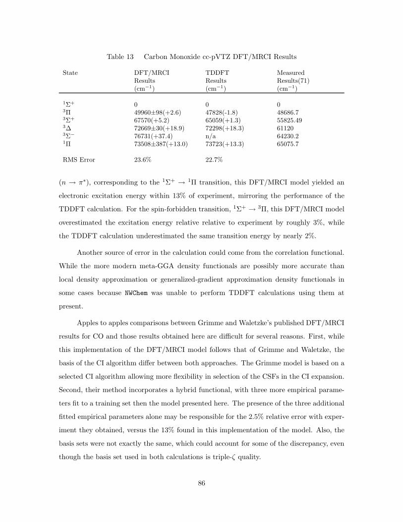
Table 13 Carbon Monoxide cc-pVTZ DFT/MRCI Results
State DFT/MRCI TDDFT MeasuredResults Results Results(71)(cm−1) (cm−1) (cm−1)
1Σ+ 0 0 03Π 49960±98(+2.6) 47828(-1.8) 48686.73Σ+ 67570(+5.2) 65059(+1.3) 55825.493∆ 72669±30(+18.9) 72298(+18.3) 611203Σ− 76731(+37.4) n/a 64230.21Π 73508±387(+13.0) 73723(+13.3) 65075.7
RMS Error 23.6% 22.7%
(n → π∗), corresponding to the 1Σ+ → 1Π transition, this DFT/MRCI model yielded an
electronic excitation energy within 13% of experiment, mirroring the performance of the
TDDFT calculation. For the spin-forbidden transition, 1Σ+ → 3Π, this DFT/MRCI model
overestimated the excitation energy relative relative to experiment by roughly 3%, while
the TDDFT calculation underestimated the same transition energy by nearly 2%.
Another source of error in the calculation could come from the correlation functional.
While the more modern meta-GGA density functionals are possibly more accurate than
local density approximation or generalized-gradient approximation density functionals in
some cases because NWChem was unable to perform TDDFT calculations using them at
present.
Apples to apples comparisons between Grimme and Waletzke’s published DFT/MRCI
results for CO and those results obtained here are difficult for several reasons. First, while
this implementation of the DFT/MRCI model follows that of Grimme and Waletzke, the
basis of the CI algorithm differ between both approaches. The Grimme model is based on a
selected CI algorithm allowing more flexibility in selection of the CSFs in the CI expansion.
Second, their method incorporates a hybrid functional, with three more empirical parame-
ters fit to a training set then the model presented here. The presence of the three additional
fitted empirical parameters alone may be responsible for the 2.5% relative error with exper-
iment they obtained, versus the 13% found in this implementation of the model. Also, the
basis sets were not exactly the same, which could account for some of the discrepancy, even
though the basis set used in both calculations is triple-ζ quality.
86
Boron Fluoride. Table 14 lists DFT/MRCI, TDDFT, and measured results for the
boron fluoride molecule at a bond length of 1.262 A, obtained from diatomic spectroscopic
measurements by Herzberg (67). This DFT/MRCI calculation used references from an
active space defined by a 8 electron, 6 orbital full valence CAS over the boron and fluorine
2s and 2p orbitals, with the 41 highest energy virtual orbitals frozen. The Kohn-Sham
orbital energy difference between HOMO and the first frozen virtual orbital was roughly 38
eV. This expansion involved 206,346 CSFs. Without freezing the virtual orbitals, the BF
expansion size was over 9 million CSFs. Here, the DFT/MRCI approach to freezing virtual
orbitals resulted in a reduction in the CI expansion size of a factor of 46. Shape-consistent
RECPs were used on both boron and fluorine, along with the corresponding spin-orbit
operators, in order to obtain a relativistic treatment for both boron and fluorine. Both
RECPs had the 1s electrons in the core.
The boron fluoride diatomic was investigated in the Kleinschmidt et al paper (76).
They used a shape-consistent relativistic effective core potential was used along with a spin-
orbit operator. A cc-pVTZ quality basis set was used in their boron fluoride calculation.
Table 14 BF cc-pVTZ DFT/MRCI Results
State DFT/MRCI TDDFT ExperimentResults Results Results(71)(cm−1) (cm−1) (cm−1)
1Σ+ 0 0 0
3Π2 28500±218(-2.2)3Π1 30629±166(+5.0) 22329(+23.4) 29144.33Π+
0 ,3Π−
0 32057±154(+10.0)
1Π 55798±618(+9.1) 54452(+6.4) 51157.453Σ+ 68893(+4.7) 69983(+14.7) 61035.31Σ+ 71683(+9.7) 90809(+31.6) 65353.93Σ+ 65526(-2.3) 78023(+16.4) 67045
RMS Error 18.3% 45.5%
Kleinschmidt et al reported a DFT/MRCI result of 27831 cm−1 for the 1Σ+ to 3Π excitation
(76). Using a two-step method to compute spin-orbit matrix elements, they obtained a spin-
87
orbit splitting of the 3Π state of 22.3 cm−1. They do not report a TDDFT excitation energy.
They reported no other state excitation energies.
A MR-SOCISD calculation without DFT on the same active space produces a spin-
orbit splitting in the 3Π state of 22.7 cm−1. The DFT/MRCI calculated spin-orbit splitting
between the 3Π2 and 3Π1 states was roughly 2129 cm−1, while the calculated splitting
between the 3Π1 and 3Π0+ and 3Π0− states was 1428 cm−1, nearly two orders of magni-
tude greater than the MR-SOCISD calculation and the Kleinschmidt et al results. There
are two possible reasons for this dramatic overestimation of the spin-orbit spitting in the
DFT/MRCI results. The first reason is most likely due to degeneracy errors introduced by
the DFT/MRCI method. The result of this state-broadening is to lift the degeneracies in
eigenvalues, introducing a source of error into the calculation. For the boron fluoride ex-
ample above, the degeneracy error introduced into the 3Π states amounts to approximately
180 cm−1 on average, potentially swamping out the very small spin-orbit splitting. This de-
generacy error suggests that this particular implementation of DFT/MRCI will not perform
well when computing small spin-orbit splittings. Approximate degeneracy is maintained by
the DFT/MRCI method in most cases, but the CI calculation can not restore eigenvalue
degeneracies once they have been broken. The second possible reason for the large spin-orbit
splitting error in the DFT/MRCI calculation is possibly due an overestimation of the ex-
pectation value of S2 on wave functions formed from Kohn-Sham orbitals. This is a known
feature of Kohn-Sham orbitals. The fact that the expectation value of S2 from restricted
and unrestricted self-consistent field calculations can be too large by up to several percent
(135). This affects spin-orbit matrix elements over these spin-adapted CSFs, in that the
contributions from S+, S−, and Sz can all be overestimated by a small amount.
For example, an unrestricted Kohn-Sham doublet wave function with an S2 expec-
tation value of 0.7618 overestimates the expectation value by nearly 1.6%. This results in
a value for Sz of 0.5058, a result in error by nearly 1.2%. This 1% error in Sz then gets
directly factored into the LzSz contribution to the spin-orbit matrix element. Similar errors
propagate into the spin-orbit matrix elements from the S+ and S− contributions. Worse
case scenario, these errors are all on the order of 1 to 2%, with no cancelation, yielding a
spin-orbit matrix element in error by roughly 3 to 4%.
88

It is important to note that the calculation by Kleinschmidt et al computed the spin-
orbit coupling in a two-step procedure, after the DFT/MRCI calculation on the singlet
ground state and triplet excited state had already been performed separately. Scalar rela-
tivistic effects were not included in their calculation.
In this calculation, however, both scalar relativistic and spin-orbit effects were in-
cluded in the DFT/MRCI calculation, the first such calculation performed. The relative
error obtained in the calculation for the excitation from the 1Σ+ → 3Π state was nearly
4.3% when compared with experiment when the 3Π state energies were averaged, and the
DFT/MRCI calculation outperformed the TDDFT calculation when comparing the RMS
errors over all six states computed. However, the spin-orbit splitting of the 3Π state was
grossly overestimated by this DFT/MRCI model. The error in the TDDFT calculation for
the 1Σ+ → 3Π excitation was in error by roughly 23%.
Bromine Atom. The bromine atom was chosen to provide a test of the spin-
orbit DFT/MRCI method using a fairly heavy atom. Spin-orbit coupling splits the doublet
P ground state arising from a p5 electron configuration into the ground state 2P 3
2
and
unoccupied 2P 1
2
state. Spin-orbit effects are largest in P states, and the splitting observed
in bromine atomic spectroscopy is on the order of 3600 cm−1. Non spin-orbit calculations
will be unable to resolve this splitting, producing only a single energy for the 2P state.
The original DFT/MRCI method proposed by Grimme and Waletzke can not perform
this calculation, as their original method did not incorporate two-component relativistic
effects. The method extension published by Kleinschmidt et al introduces spin-orbit effects
(but not scalar relativistic effects), and is multiplicity limited in the same way as the original
Grimme and Waletzke procedure to coupling between singlet and triplet states only.
Since the bromine atom ground state is an open p5 electronic configuration, with
an odd number of electrons, the electronic states will transform according to the extra
irreducible representations of the double group. This calculation represents the first ap-
plication of a DFT/MRCI method to an odd-electron state, incorporating both one- and
two-component relativistic effects.
89
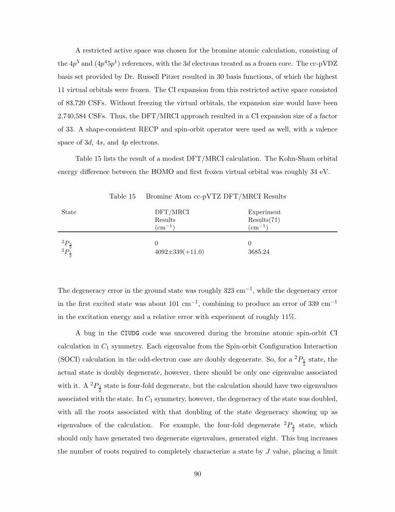
A restricted active space was chosen for the bromine atomic calculation, consisting of
the 4p5 and (4p45p1) references, with the 3d electrons treated as a frozen core. The cc-pVDZ
basis set provided by Dr. Russell Pitzer resulted in 30 basis functions, of which the highest
11 virtual orbitals were frozen. The CI expansion from this restricted active space consisted
of 83,720 CSFs. Without freezing the virtual orbitals, the expansion size would have been
2,740,584 CSFs. Thus, the DFT/MRCI approach resulted in a CI expansion size of a factor
of 33. A shape-consistent RECP and spin-orbit operator were used as well, with a valence
space of 3d, 4s, and 4p electrons.
Table 15 lists the result of a modest DFT/MRCI calculation. The Kohn-Sham orbital
energy difference between the HOMO and first frozen virtual orbital was roughly 34 eV.
Table 15 Bromine Atom cc-pVTZ DFT/MRCI Results
State DFT/MRCI ExperimentResults Results(71)(cm−1) (cm−1)
2P 3
2
0 02P 1
2
4092±339(+11.0) 3685.24
The degeneracy error in the ground state was roughly 323 cm−1, while the degeneracy error
in the first excited state was about 101 cm−1, combining to produce an error of 339 cm−1
in the excitation energy and a relative error with experiment of roughly 11%.
A bug in the CIUDG code was uncovered during the bromine atomic spin-orbit CI
calculation in C1 symmetry. Each eigenvalue from the Spin-orbit Configuration Interaction
(SOCI) calculation in the odd-electron case are doubly degenerate. So, for a 2P 1
2
state, the
actual state is doubly degenerate, however, there should be only one eigenvalue associated
with it. A 2P 3
2
state is four-fold degenerate, but the calculation should have two eigenvalues
associated with the state. In C1 symmetry, however, the degeneracy of the state was doubled,
with all the roots associated with that doubling of the state degeneracy showing up as
eigenvalues of the calculation. For example, the four-fold degenerate 2P 3
2
state, which
should only have generated two degenerate eigenvalues, generated eight. This bug increases
the number of roots required to completely characterize a state by J value, placing a limit
90
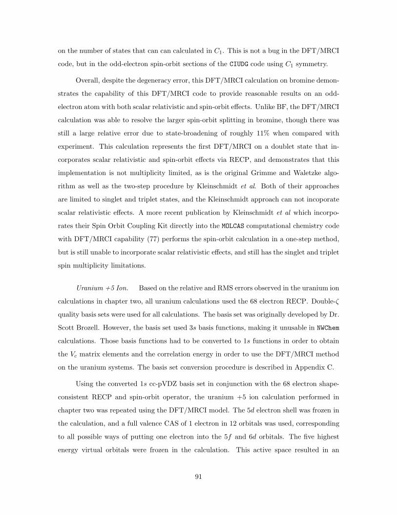
on the number of states that can can calculated in C1. This is not a bug in the DFT/MRCI
code, but in the odd-electron spin-orbit sections of the CIUDG code using C1 symmetry.
Overall, despite the degeneracy error, this DFT/MRCI calculation on bromine demon-
strates the capability of this DFT/MRCI code to provide reasonable results on an odd-
electron atom with both scalar relativistic and spin-orbit effects. Unlike BF, the DFT/MRCI
calculation was able to resolve the larger spin-orbit splitting in bromine, though there was
still a large relative error due to state-broadening of roughly 11% when compared with
experiment. This calculation represents the first DFT/MRCI on a doublet state that in-
corporates scalar relativistic and spin-orbit effects via RECP, and demonstrates that this
implementation is not multiplicity limited, as is the original Grimme and Waletzke algo-
rithm as well as the two-step procedure by Kleinschmidt et al. Both of their approaches
are limited to singlet and triplet states, and the Kleinschmidt approach can not incoporate
scalar relativistic effects. A more recent publication by Kleinschmidt et al which incorpo-
rates their Spin Orbit Coupling Kit directly into the MOLCAS computational chemistry code
with DFT/MRCI capability (77) performs the spin-orbit calculation in a one-step method,
but is still unable to incorporate scalar relativistic effects, and still has the singlet and triplet
spin multiplicity limitations.
Uranium +5 Ion. Based on the relative and RMS errors observed in the uranium ion
calculations in chapter two, all uranium calculations used the 68 electron RECP. Double-ζ
quality basis sets were used for all calculations. The basis set was originally developed by Dr.
Scott Brozell. However, the basis set used 3s basis functions, making it unusable in NWChem
calculations. Those basis functions had to be converted to 1s functions in order to obtain
the Vc matrix elements and the correlation energy in order to use the DFT/MRCI method
on the uranium systems. The basis set conversion procedure is described in Appendix C.
Using the converted 1s cc-pVDZ basis set in conjunction with the 68 electron shape-
consistent RECP and spin-orbit operator, the uranium +5 ion calculation performed in
chapter two was repeated using the DFT/MRCI model. The 5d electron shell was frozen in
the calculation, and a full valence CAS of 1 electron in 12 orbitals was used, corresponding
to all possible ways of putting one electron into the 5f and 6d orbitals. The five highest
energy virtual orbitals were frozen in the calculation. This active space resulted in an
91

expansion size of 39,836 CSFs. The size of the CI expansion without the frozen virtuals was
1,813,300 CSFs. The DFT/MRCI approach resulted in a reduction in the CI expansion size
of a factor of 46. Table 16 lists the results of the DFT/MRCI calculation, along with the
corresponding MR-SOCISD calculation using the 3sd basis and the experimental values.
Table 16 U5+ DFT/MRCI Results, (5f6d)1 Reference Space
DFT/MRCI MR-SOCISD68e 68e
Principle RECP 1s RECP 3sdLS cc-pVDZ cc-pVDZ Experiment(17)Component (cm−1) (cm−1) (cm−1)
2Fo5
2
0 0 02Fo
7
2
6515±109(-14.4) 7578(-0.4) 7608.6
The degeneracy error in the 2F o5
2
ground state amounted to nearly 71 cm−1. Degeneracy
error in the 2F o7
2
first excited state was roughly 82 cm−1. Combining the ground-state and
first excited state degeneracy errors resulted produced an error in the excitation energy of
109 cm−1, yielding a relative error with experiment of 14%.
As in the case with the bromine calculation, the large spin-orbit splitting in the 2F
ground state, measured to be 7608.6 cm−1, was resolvable by this DFT/MRCI method.
Again, the C1 odd-electron bug in the CIUDG code doubled the expected degeneracies of the
ground and first excited states, requiring the calculation of 28 eigenvalues to fully resolve
them. The 2F 5
2
ground state required 12 eigenvalues to characterize, while the 2F 7
2
first
excited state required 16 eigenvalues to fully characterize by J value. The hard limit on
number of eigenvalues in the CIUDG code is 39, which would make exploring more excited
states of the uranium +5 ion difficult.
Because of the limit of 39 eigenvalues in the CIUDG code, the next expected excited
state, 2D 3
2
, would push the number of required roots to 36. This is the limit on the number
of states that can be examined with this version of the DFT/MRCI model. The reduced
number of 3d basis functions and the effect of the degeneracy errors are expected to result
92
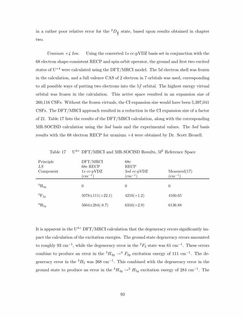
in a rather poor relative error for the 2D 3
2
state, based upon results obtained in chapter
two.
Uranium +4 Ion. Using the converted 1s cc-pVDZ basis set in conjunction with the
68 electron shape-consistent RECP and spin-orbit operator, the ground and first two excited
states of U+4 were calculated using the DFT/MRCI model. The 5d electron shell was frozen
in the calculation, and a full valence CAS of 2 electron in 7 orbitals was used, corresponding
to all possible ways of putting two electrons into the 5f orbital. The highest energy virtual
orbital was frozen in the calculation. This active space resulted in an expansion size of
260,116 CSFs. Without the frozen virtuals, the CI expansion size would have been 5,397,041
CSFs. The DFT/MRCI approach resulted in a reduction in the CI expansion size of a factor
of 21. Table 17 lists the results of the DFT/MRCI calculation, along with the corresponding
MR-SOCISD calculation using the 3sd basis and the experimental values. The 3sd basis
results with the 68 electron RECP for uranium +4 were obtained by Dr. Scott Brozell.
Table 17 U4+ DFT/MRCI and MR-SOCISD Results, 5f2 Reference Space
Principle DFT/MRCI 68eLS 68e RECP RECPComponent 1s cc-pVDZ 3sd cc-pVDZ Measured(17)
(cm−1) (cm−1) (cm−1)
3H4g 0 0 0
3F2g 5078±111(+22.1) 4210(+1.2) 4160.65
3H5g 5604±284(-8.7) 6316(+2.9) 6136.88
It is apparent in the U4+ DFT/MRCI calculation that the degeneracy errors significantly im-
pact the calculation of the excitation energies. The ground state degeneracy errors amounted
to roughly 93 cm−1, while the degeneracy error in the 3F2 state was 61 cm−1. These errors
combine to produce an error in the 3H4g →3 F2g excitation energy of 111 cm−1. The de-
generacy error in the 3H5 was 268 cm−1. This combined with the degeneracy error in the
ground state to produce an error in the 3H4g →3 H5g excitation energy of 284 cm−1. The
93
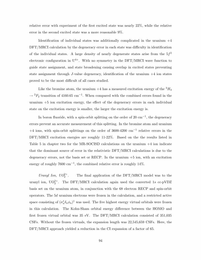
relative error with experiment of the first excited state was nearly 22%, while the relative
error in the second excited state was a more reasonable 9%.
Identification of individual states was additionally complicated in the uranium +4
DFT/MRCI calculation by the degeneracy error in each state was difficulty in identification
of the individual states. A large density of nearly degenerate states arise from the 5f2
electronic configuration in U4+. With no symmetry in the DFT/MRCI wave function to
guide state assignment, and state broadening causing overlap in excited states preventing
state assignment through J-value degeneracy, identification of the uranium +4 ion states
proved to be the most difficult of all cases studied.
Like the bromine atom, the uranium +4 has a measured excitation energy of the 3H4
→ 3F2 transition of 4160.65 cm−1. When compared with the combined errors found in the
uranium +5 ion excitation energy, the effect of the degeneracy errors in each individual
state on the excitation energy is smaller, the larger the excitation energy is.
In boron fluoride, with a spin-orbit splitting on the order of 20 cm−1, the degeneracy
errors prevent an accurate measurement of this splitting. In the bromine atom and uranium
+4 ions, with spin-orbit splittings on the order of 3600-4200 cm−1 relative errors in the
DFT/MRCI excitation energies are roughly 11-22%. Based on the the results listed in
Table 5 in chapter two for the MR-SOCISD calculations on the uranium +4 ion indicate
that the dominant source of error in the relativistic DFT/MRCI calculations is due to the
degeneracy errors, not the basis set or RECP. In the uranium +5 ion, with an excitation
energy of roughly 7600 cm−1, the combined relative error is roughly 14%.
Uranyl Ion, UO2+2 . The final application of the DFT/MRCI model was to the
uranyl ion, UO2+2 . The DFT/MRCI calculation again used the converted 1s cc-pVDZ
basis set on the uranium atom, in conjunction with the 68 electron RECP and spin-orbit
operators. The 5d uranium electrons were frozen in the calculation, and a restricted active
space consisting of (σ1uδuφu)1 was used. The five highest energy virtual orbitals were frozen
in this calculation. The Kohn-Sham orbital energy difference between the HOMO and
first frozen virtual orbital was 35 eV. The DFT/MRCI calculation consisted of 351,035
CSFs. Without the frozen virtuals, the expansion length was 22,545,659 CSFs. Here, the
DFT/MRCI approach yielded a reduction in the CI expansion of a factor of 65.
94
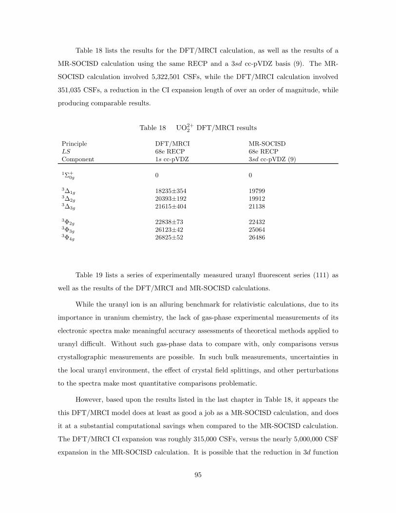
Table 18 lists the results for the DFT/MRCI calculation, as well as the results of a
MR-SOCISD calculation using the same RECP and a 3sd cc-pVDZ basis (9). The MR-
SOCISD calculation involved 5,322,501 CSFs, while the DFT/MRCI calculation involved
351,035 CSFs, a reduction in the CI expansion length of over an order of magnitude, while
producing comparable results.
Table 18 UO2+2 DFT/MRCI results
Principle DFT/MRCI MR-SOCISDLS 68e RECP 68e RECPComponent 1s cc-pVDZ 3sd cc-pVDZ (9)
1Σ+
0g 0 0
3∆1g 18235±354 197993∆2g 20393±192 199123∆3g 21615±404 21138
3Φ2g 22838±73 224323Φ3g 26123±42 250643Φ4g 26825±52 26486
Table 19 lists a series of experimentally measured uranyl fluorescent series (111) as
well as the results of the DFT/MRCI and MR-SOCISD calculations.
While the uranyl ion is an alluring benchmark for relativistic calculations, due to its
importance in uranium chemistry, the lack of gas-phase experimental measurements of its
electronic spectra make meaningful accuracy assessments of theoretical methods applied to
uranyl difficult. Without such gas-phase data to compare with, only comparisons versus
crystallographic measurements are possible. In such bulk measurements, uncertainties in
the local uranyl environment, the effect of crystal field splittings, and other perturbations
to the spectra make most quantitative comparisons problematic.
However, based upon the results listed in the last chapter in Table 18, it appears the
this DFT/MRCI model does at least as good a job as a MR-SOCISD calculation, and does
it at a substantial computational savings when compared to the MR-SOCISD calculation.
The DFT/MRCI CI expansion was roughly 315,000 CSFs, versus the nearly 5,000,000 CSF
expansion in the MR-SOCISD calculation. It is possible that the reduction in 3d function
95
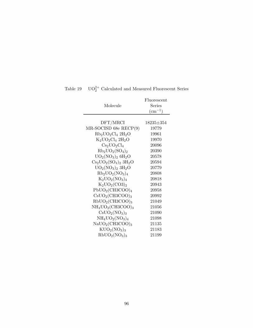
Table 19 UO2+2 Calculated and Measured Fluorescent Series
FluorescentMolecule Series
(cm−1)
DFT/MRCI 18235±354MR-SOCISD 68e RECP(9) 19779
Rb2UO2Cl4 2H2O 19961K2UO2Cl4 2H2O 19970
Cs2UO2Cl4 20096Rb2UO2(SO4)2 20390
UO2(NO3)2 6H2O 20578Cs2UO2(SO4)2 3H2O 20594
UO2(NO3)2 3H2O 20779Rb2UO2(NO3)4 20808K2UO2(NO3)4 20818K2UO2(CO3)2 20943
PbUO2(CH3COO)4 20958CsUO2(CH3COO)3 20992RbUO2(CH3COO)3 21049NH4UO2(CH3COO)3 21056
CsUO2(NO3)3 21090NH4UO2(NO3)4 21098
NaUO2(CH3COO)3 21135KUO2(NO3)3 21183RbUO2(NO3)3 21199
96
flexibility resulting from the 1s basis conversion process is responsible for more error than
degeneracy errors here, which are on the range from 42 cm−1 for the 3Φ3g state to 404 cm−1
in the 3∆3g state. Despite this, the DFT/MRCI results fall nicely in range of measured
uranyl spectra listed in Table 19. One possible explanation is that some cancellation of
error occurred in the linear molecular calculation that was not present in the spherically
symmetric ionic calculations. The calculated excitation energies for the fluorescent spectra
fall in the low end of the measured values. A likely reason for the measured values being
higher is because of solvation or crystal field effects that are not present in the theoretical
gas phase calculations.
97
IV. Conclusions
This chapter contains an analysis of the results of the various aspects of this research project,
as well conclusions based upon that analysis. It is divided into several sections, one section
for each major thrust of this project.
The first section analyzes and draws conclusions from the series of MR-SOCISD cal-
culations on the uranium +5 and uranium +4 ions described in chapter two. Conclusions
based on the relative errors involved in the various core-valence cut-off choices using the
shape-consistent RECPs are drawn. The second section examines the overall performance
of this implementation of the DFT/MRCI model, and based on the analysis in the previous
chapter, examines the observed successes in the calculations on carbon monoxide, boron
fluoride, the bromine atom, followed by a discussion of performance of the DFT/MRCI
model on uranium ions and molecules. Next the successes and failures in achieving the re-
search objectives laid out in chapter one will be covered, followed finally by suggestions for
future work in the area of hybrid DFT and wave function based computational chemistry
for application to atomic and molecular excited states.
Uranium Shape-Consistent RECP Accuracy Assessment
Two factors impacting the relative and overall errors in the calculation of the electronic
excitation energies of the U5+ and U4+ cations are the sizes of the relativistic effective
potential core and the reference space.
The effect of the core size in the uranium cation calculations shows that the 68 electron
core does well in both the 5fn and (5f6d)n reference spaces when compared with experi-
ment. States that arise from electron configurations not included in the reference space were
poorly modeled in all calculations and skew the overall RMS error accordingly. These states
are the 2D and 2S states in the U5+ calculations, which arise from 6d1 and 7s1 electron
configurations, respectively. Similarly, the odd states in the U4+ calculations, arising from
5f16d1 electron configurations are not modeled well using only the 5f2 references.
The larger error in those states can be explained by the fact excitations from electron
configurations specifically in the reference space represent excitation levels higher than single
and double excitations. For example, states produced by 6d1 configurations are computed
98
at the single and double excitation level when using a smaller 5f1 reference space, however,
these same states contain selected contributions of higher order (triple and quadruple) exci-
tations from the larger (5f6d)1 active space. Thus, the 2D states are computed at excitation
levels higher than singles and doubles when computed using the larger active space.
With respect to the choice of the core size, in both uranium cation calculations, the 68
electron core produced the lowest relative and RMS errors, on the order of 1-2% for those
states included in the reference space in the U5+ calculations. The 78 electron core produces
large relative and RMS errors in the U5+ calculation. The 60 electron core produces better
results when compared with the 78 electron core, however, the accuracies produced by the
60 electron core do not warrant the larger computational effort in terms of CI expansion
size involved in its use.
For the +4 cation, however, different results were obtained. When examining only the
even states arising from the 5f2 configurations, both the 68 and 78 electron core calcula-
tions produced roughly equivalent results, both of which outperform the 60 electron core.
Inclusion of the odd states arising from 5f16d1 electronic configurations skew the overall
errors in favor of the 68 electron core.
One possible explanation for the relative success of the 68 electron core RECP in the
U5+ calculation may lie in the nature of the core and valence electron shell treatments.
Recall the various valence electrons included in each RECP listed in table 1. Incorporation
of an electron shell in the core allows for a relativistic treatment (relativistic contraction
and expansion, as well as spin-orbit splitting) of those electrons, while relativity is treated
indirectly, via interaction with the core potential, in the valence electrons. Electrons in the
core p-shells are known to exhibit the largest spin-orbit spitting, so inclusion of the uranium
5p shell in the core in order for an accurate relativistic description seems warranted, as
is done in the 68 and 78 electron core potentials. Removal of the uranium 5d shell from
the valence space, as is done in the 78 electron shape-consistent core potential, does not
allow for relaxation of the 6d electron shell. The 68 electron core RECP strikes one possible
balance between relativity and polarization. The near degeneracy of the 5f and 6d shells in
many uranium atomic species seems to require an accurate treatment of the 6d electronic
99
excitations, which can be facilitated by freeing the 5d shell from the core and into the valence
electron space.
The similar performance of the 78 and 68 electron cores in the U4+ calculations seems
to counter the argument presented above. One possible source of this result is the fact that
in this core potential treatment, there are no core-valence interactions possible, so the shape-
consistent core potential method does not include any way for the core region to polarize.
Thus, while the 68 electron core allows polarization of the 5d electrons, with only indirect
relativistic effects via interaction with the core, the 78 electron core allows a relativistic
treatment of the 5d electrons, but no polarization to occur. One possible explanation of
the observed results is that these treatments are roughly the same magnitude, and that a
higher order description of the core-valence interaction may be necessary to resolve the near
degeneracy in the 68 and 78 electron core results. The fact remains, however, that the 78
electron core calculations represent a lower computational cost in terms of CI expansion
length, and give accurate results, in the U4+ calculations. The presence of a trend may be
established by examining the U3+ and U2+ cations.
Overall, applying Christiansen et al shape-consistent relativistic effective core poten-
tials in MR-SOCISD calculations of the ground and excited states of U5+ and U4+ ions
shows that the 68 electron RECP, along with a cc-pVDZ basis set, yields relative errors
of 1 to 3% with experiment for each calculated state, part of which may be due to a for-
tuitous cancellation of error based on analysis of results obtained using double-ζ quality
basis sets. The lowest relative errors in excitation energies were achieved when the refer-
ence space included all the electron configurations spawning the states of interest. Inclusion
of the spin-orbit interaction is crucial in these calculations, as the lowest energy electronic
transitions in U5+ and U4+ arise from 5f → 5f transitions.
DFT/MRCI Model
The first experiences with applications of this implementation of the DFT/MRCI
model was during the determination of the damping parameters p1 and p2. The training
systems, listed in Appendix B, span the first two rows of the periodic table, with emphasis
on atomic systems with open 2p shells using double-ζ quality basis sets.
100
It is interesting to note the absolute errors for each individual test case listed in
Appendix B vary. In some cases, the error between the DFT/MRCI and FCI results are
very small, on the order of micro-Hartrees. Even the largest errors obtained are not greater
than 10s of milliHartrees. It is impressive that the hybrid DFT/CI method implemented
here can achieve such accuracies when compared with FCI calculations, which are known
to be the exact non-relativistic solution for that particular basis set. All training systems
listed in Appendix B were treated non-relativistically.
When examining the density plots of in Appendix B, some are devoid of features. The
beryllium cc-pVDZ calculation is one such example. The triple-ζ calculation reveals more
detail in the p1/p2 space, where the double-ζ basis set calculation shows no features at all.
Helium is another such example where the larger basis set reveals detail in the damping
parameter space that is absent in the calculation with the smaller basis set. In all cases
where there were double- and triple-ζ quality basis set calculations on the same system, the
larger basis set revealed as much and usually more detail in the damping parameter space.
Unfortunately, for the larger atoms, beyond carbon, FCI calculations using larger basis sets
simply were not feasible in this research effort.
Examining the density plots in Appendix B, several of the calculations reveal interest-
ing structure. Some density plots revealed contours similar in shape to those found in the
analytical investigation of the two level system investigated in chapter three. Double-ζ H2,
the helium atom at both basis set sizes, oxygen and fluorine all exhibit this simple structure.
Most of the other density plots showed band-like structure in the damping parameter space.
In most cases where this minimum error banding occurred, the bands tended to stabilize at
higher values of p2, as if exhibiting asymptotic behavior. It is difficult to draw overarching
significance to this banded structure in the damping parameter space, as little is known
about the theoretical basis of the DFT/MRCI method. One of the most interesting band
structures is seen in the case of the beryllium dimer. There does appear to be some corre-
lation between the banding structure in the density plots and the single reference nature of
the test system involved. Both the beryllium atom (cc-pVTZ) and beryllium dimer have the
most multi-determinant character, and both exhibit interesting banding structure. Carbon,
nitrogen, and boron also have larger multi-reference character than the other systems, and
they exhibit banding in the density plots. It is possible, at least in the plots that show fea-
101

tures (cc-pVDZ helium and beryllium are relatively featureless) in the damping parameter
space, that all of the plots show banding, however, the location and direction of the bands
varies from system to system. In some systems, such as lithium, the band runs up the right
hand side of the density plot, and is independent of p2. In other cases, such as neon, the
band runs up the left hand side of the density plot, apparently independent of p2. Perhaps
in these cases, which are mostly single-determinant systems, forming a CI expansion based
upon those Kohn-Sham orbitals results in a good initial guess, which is then only corrected
through small contributions from degenerate CSFs. In the cases of oxygen and fluorine,
it appears that the DFT/MRCI approach using a GGA correlation functional may not be
accurate enough to show the banding structure, based on the similarities with the absolute
error density plots of the two level system investigated in detail in Appendix B. A rigor-
ous theoretical basis for the hybrid DFT/MRCI method should be able to account for this
banding structure. At the moment, however, only loose trends can be drawn from the data
in Appendix B. Whether these trends can be attributed to the accuracy of the correlation
functional, the basis set quality, or, the multi-determinant nature of the system studied is
difficult to determine at this stage.
Three systems were chosen to demonstrate the capabilities of this implementation of
this DFT/MRCI model: Carbon monoxide, boron fluoride, and the bromine atom. Car-
bon monoxide and boron fluoride were chosen to compare the accuracy of this model with
published results of Grimme and Waletzke for carbon monoxide, and Kleinschmidt et al for
boron fluoride. The carbon monoxide calculation did not involve relativistic effects. The
DFT/MRCI method resulted in a reduction in the CI expansion size in both CO and BF of
over a factor of 40.
Using the damping parameters found from the training set using calculations involving
the first two rows on the periodic table, the carbon monoxide calculations performed here
seem to agree in principle with those results obtained by Grimme and Waletzke. Results
listed in Table 13 show reasonable agreement between the DFT/MRCI results and the
TDDFT results. The DFT/MRCI model outperforms TDDFT for nearly every state and
in overall RMS error, slightly skewed by the large error in the 3Σ− state, which may be
misidentified in the correspondence with experiment. For the excitation published, the
allowed (n → π∗), corresponding to the 1Σ+ → 1Π transition, this DFT/MRCI model
102

yielded an electronic excitation energy within 12% of experiment, mirroring the performance
of the TDDFT calculation. For the spin-forbidden transition, 1Σ+ → 3Π, this DFT/MRCI
model overestimated the excitation energy relative relative to experiment by roughly 1%,
while the TDDFT calculation underestimated the same transition energy by nearly 2%.
Another source of error in the calculation could be the correlation functional used.
Modern meta-GGA density functionals are possibly more accurate than local density ap-
proximation or generalized-gradient approximation density functionals in some cases.
Apples to apples comparisons between Grimme and Waletzke’s published DFT/MRCI
results for CO and those results obtained here are difficult for several reasons. First, while
this implementation of the DFT/MRCI model follows that of Grimme and Waletzke, the
basis of the CI algorithm differ between both approaches. The Grimme model is based on a
selected CI algorithm, allowing more flexibility in selection of the CSFs in the CI expansion.
Second, their method incorporates a hybrid functional, with three more empirical parame-
ters fit to a training set then the model presented here. The presence of the three additional
fitted empirical parameters alone may be responsible for the 2.5% relative error with exper-
iment they obtained, versus the 12% found in this implementation of the model. Also, the
basis sets were not exactly the same, which could account for some of the discrepancy, even
though the basis set used in both calculations are of triple-ζ quality.
The DFT/MRCI calculation on boron fluoride performed here was an attempt to
duplicate the results obtained by Kleinschmidt et al using the relativistic capabilities of the
COLUMBUS code in conjunction with the DFT/MRCI model. It is important to note that
the calculation by Kleinschmidt et al involved only computing the spin-orbit coupling in a
two-step procedure, after the DFT/MRCI calculation on the singlet ground state and triplet
excited state had already been performed. Scalar relativistic effects were not included in
their calculation.
In this calculation, however, both scalar relativistic and spin-orbit effects were included
in the DFT/MRCI calculation, the first such calculation performed. While the relative
error obtained in the calculation for the excitation from the 1Σ+ → 3Π state was nearly
22% when compared with experiment, and the DFT/MRCI calculation outperformed the
TDDFT calculation when comparing the RMS errors over all six states computed. However,
103
the spin-orbit splitting of the 3Π state was grossly overestimated by this DFT/MRCI model.
There are two possible contributing factors to this large spin-orbit splitting error in the BF
calculation. First, state broadening is introduced by the DFT/MRCI method. The result
of this state-broadening is to lift the degeneracies in eigenvalues, introducing a source of
error into the calculation. For the boron fluoride example above, the state broadening error
introduced into the 3Π state is roughly 115 cm−1, potentially swamping out the very small
spin-orbit splitting. This degeneracy error suggests that this particular implementation of
DFT/MRCI will not perform well when computing small spin-orbit splittings. Kleinschmidt
et al reported a spin-orbit splitting of about 22 cm−1, a result verified through a small MR-
SOCISD calculation.
The degeneracy errors arise from two sources. The first source is the broken degeneracy
in the initial Kohn-Sham orbitals, problematic for DFT calculations and atomic calculations
with d orbitals and above. This is due to the fact that the approximate density functionals
are not yet capable of reproducing the degeneracy in spherically symmetric states with
angular momentum L = 2 or higher. The second degeneracy error source is the DFT/MRCI
method, which was shown in chapter three to be capable of breaking degeneracies between
eigenvalues. Approximate degeneracy is maintained by the DFT/MRCI method in most
cases, but the CI calculation can not restore proper eigenvalue degeneracies if they are
broken in the initial guess. The second possible reason for the large spin-orbit splitting
error in the DFT/MRCI calculation is possibly due an overestimation of the expectation
value of S2 on wave functions formed from Kohn-Sham orbitals. It is a known feature of
Kohn-Sham orbitals (135) that the expectation value of S2 from restricted and unrestricted
self-consistent field calculations are too large by up to several percent. This affects spin-
orbit matrix elements over these spin-adapted CSFs, in that the contributions from S+, S−,
and Sz can be overestimated by a small amount. Worse case scenario, these errors are all
on the order of 1 to 2% with no cancellation, yielding a spin-orbit matrix element in error
by roughly 6 to 7%.
In terms of correspondence with the measured experimental excitation energy, the
DFT/MRCI calculation was able to predict the 3Π excitation energy to less than 22%,
with a very small CI expansion of less than 20,000 CSFs, however degeneracy errors made
104
an accurate spin-orbit splitting calculation impossible for this system. The corresponding
relative error in the TDDFT calculation was 23.4%.
The bromine atom is an odd-electron system, with a 2P ground state. It is a fairly
heavy atom with a spin-orbit splitting of the ground state which is two orders of magnitude
higher than in BF. Indeed, experiment measures a spin-orbit splitting in the 2P state of
about 3600 wave numbers.
A bug in the odd-electron, spin-orbit behavior of the CIUDG code was uncovered which
resulted in a doubling of the degeneracies of the calculated eigenvalues in C1 symmetry.
This bug increases the number of roots required to completely characterize a state by J
value, placing a limit on the number of states that can can calculated in C1. This is not a
bug in the DFT/MRCI code, but in the odd-electron spin-orbit sections of the code in C1
symmetry.
The degeneracy error in the Br ground state was roughly 323 cm−1, while the de-
generacy error in the first excited state was about 102 cm−1, yielding a relative error with
experiment of 11%. Overall, despite the degeneracy error, this DFT/MRCI calculation on
bromine demonstrates the capability of this DFT/MRCI code to provide reasonable results
on an odd-electron atom with both scalar relativistic and spin-orbit effects. Unlike BF, the
DFT/MRCI calculation was able to resolve the larger spin-orbit splitting in bromine, though
there was still a large relative error due to state-broadening of roughly 11% when compared
with experiment. This calculation represents the first DFT/MRCI on a doublet state that
incorporates scalar relativistic and spin-orbit effects via RECP, and demonstrates that this
implementation is not multiplicity limited, as are the original Grimme and Waletzke codes,
which are unable to incorporate scalar relativistic effects, and the two-step procedure by
Kleinschmidt et al. Both the Grimme and Waletzke and Klienschmidt et al DFT/MRCI
model implementations are limited to singlet and triplet states. A more recent publication
by Kleinschmidt et al which incorporates their Spin Orbit Coupling Kit directly into the
MOLCAS computational chemistry code with DFT/MRCI capability (77) performs the spin-
orbit calculation in a one-step method, but is still unable to incorporate scalar relativistic
effects, and it still has the singlet and triplet spin multiplicity limitations. The DFT/MRCI
105
approach here in the bromine calculation yielded a reduction in the CI expansion size of a
factor of 33.
Based upon the analysis in Appendix C, the basis set conversion procedure used to
create a useful 1s function basis set for use in DFT/MRCI calculations resulted in an
adequate cc-pVDZ basis set, but reduced in size from the original 3sd basis. Most of the
basis set reduction occurred in the elimination of 3d functions, reducing the flexibility of the
basis set somewhat. Calculations using both the 1s and 3sd basis set showed little impact
in the f → f transitions characteristic in the electronic spectra of the uranium +5 and +4
ions. In the +5 ion, both basis sets produced relative errors of less than 1% in 2F 5
2
→ 2F 7
2
transition. The effect of the conversion process became apparent in the D and S states.
The effect was particularly pronounced in the S state, with a relative error of nearly 37% in
the converted 1s basis set versus 10% in the original 3sd basis set. Based on this analysis,
it is assumed that the states arising from 5f configurations are relatively unaffected by the
conversion process.
As in the case with the bromine calculation, the large spin-orbit splitting in the 2F
ground state, measured experimentally to be 7608.6 cm−1, was resolvable by this DFT/MRCI
method. Again, the C1 odd-electron bug in the CIUDG code doubled the expected degen-
eracies of the ground and first excited states, required calculation of 28 eigenvalues to fully
resolve them. The 2F 5
2
ground state required 12 eigenvalues to characterize, while the 2F 7
2
first excited state required 16 eigenvalues to fully characterize.
Degeneracy errors in the 2F 5
2
ground state amounted to nearly 71 cm−1. Degeneracy
error contributed roughly 82 cm−1 to the 2F 7
2
excited state. Combining the ground state and
first excited state error statistically, the DFT/MRCI model underestimates the excitation
energy calculation climbs by about 14%. Cancellation of errors could account for the reduced
relative error in the maximum excitation energy listed in Table 16. The next expected
excited state, the 2D 3
2
would push the number of required eigenvalues to 36. This is the
limit on the number of states that can be examined with this version of the DFT/MRCI
model, because 39 eigenvalues is the hard coded limit in CIUDG.
106
The U5+ active space resulted in an expansion size of 39,836 CSFs. The size of the
CI expansion without the frozen virtuals was 1,813,300 CSFs. The DFT/MRCI approach
resulted in a reduction in the CI expansion size of a factor of 46.
It is apparent in the U4+ DFT/MRCI calculation that the state broadening intro-
duces a significant error into the calculation of the excitation energies. The combined 3H4
ground state and 3F2 degeneracy errors yield an overestimation of the excitation energy by
a slightly more than 22%. The second excited state transition energy is underestimated by
a 9%. This result was achieved with a CI expansion size of 260,116 CSFs. Without the
frozen virtuals, the CI expansion size would have been 5,397,041 CSFs. In the DFT/MRCI
approach resulted in a reduction in the CI expansion size of a factor of 21.
An additional complication in the uranium +4 DFT/MRCI calculation was that the
degeneracy error in each state complicated identification of the individual states. A large
density of nearly degenerate states arise from the 5f2 electronic configuration in U4+. The
main difficulties in state identification were due to lack of symmetry in the DFT/MRCI
wave function and state broadening overlap in excited states. Both factors complicated
state assignment through J degeneracy.
The uranium +4 has a measured excitation energy of the 3H4 → 3F2 transition of
4160.65 cm−1. When compared with the combined errors found in the uranium +5 ion
excitation energy, the effect of the degeneracy errors in each individual state on the excitation
energy is smaller, the larger the excitation energy is. This trend, based on the boron fluoride,
bromine atom, uranium +4, and uranium +5 ion DFT/MRCI results is supported by the
calculations.
In boron fluoride, with a small spin-orbit splitting on the order of 20 cm−1, degen-
eracy errors prevent an accurate measurement of this splitting. In the bromine atom and
uranium +4 ions, with spin-orbit splittings on the order of 3600-4200 cm−1, relative errors
in the DFT/MRCI excitation energies are roughly 11-22%. In the uranium +5 ion, with an
excitation energy of roughly 7600 cm−1, the combined relative error is roughly 14%. Based
on the the results in chapter two for the MR-SOCISD calculations on the uranium +4 and
+5 ions, the dominant source of error in the relativistic DFT/MRCI calculations appears
to be due to the degeneracy error.
107
The final application of this DFT/MRCI model to the uranyl ion shows that this
method holds promise, while the uranium ionic calculations showed large relative errors
with experiment in the first excitation energy.
Based upon the results listed in the last chapter in Table 18, it appears the this
DFT/MRCI model does at least as good a job as a MR-SOCISD calculation, and does
it at a substantial computational savings when compared to the MR-SOCISD calculation.
The DFT/MRCI CI expansion was roughly 315,000 CSFs, versus the over 22,000,000 CSFs
resulting from no frozen virtual orbitals. Here, the DFT/MRCI method yielded a reduction
in the CI expansion by a factor of 65. It is possible that the reduction in 3d function
flexibility resulting from the 1s basis conversion process is responsible for more error than
degeneracy errors here, which are on the range from 42 cm−1 for the 3Φ3g state to 404 cm−1
in the 3∆3g state. Despite this, the DFT/MRCI results fall nicely in the range of measured
uranyl spectra listed in Table 19. One possible explanation is that some cancellation of
error occurred in the linear molecular calculation that was not present in the spherically
symmetric ionic and atomic calculations. The calculated values for the fluorescent spectra
fall in the low end of the measured values. A likely reason for the measured values being
higher is because of solvation or crystal field perturbations that are not present in the
theoretical gas phase calculations.
Research Objective Successes and Failures
The focus of this work was to develop an accurate and scalable method for com-
puting the electronic spectra of heavy element compounds which incorporates one- and
two-component relativistic effects based upon the hybrid DFT-CI method developed by
Grimme and Waletzke (62) (63).
By leveraging the relativistic capabilities in the COLUMBUS relativistic quantum chem-
istry code, these objectives were successfully completed, as demonstrated by the boron
fluoride, bromine atom, uranium +4 and +5 ions, as well as the uranyl ion. Scalar relativis-
tic effects were incorporated through the use of shape consistent RECPs, while spin-orbit
effects were incorporated in a one-step fashion through the use of spin-orbit operators.
108
This DFT/MRCI model achieved modest accuracy when computing electronic exci-
tation energies, and consistently outperformed TDDFT calculations of the same excitation
energy. Errors in eigenvalue degeneracies, also referred to as state broadening, governed the
overall accuracy achievable in the electronic excitation energy in states split by a spin-orbit
Hamiltonian. For boron fluoride, with a spin-orbit splitting in the 3Π state of roughly 20
cm−1, as determined by MR-SOCISD calculations and obtained in reference (76), these
state broadening errors prevented accurate measurement of the spin-orbit splitting. This
model was unable to resolve the splitting, grossly overestimating the spin-orbit splitting by
several orders of magnitude. It should be noted that the measured spectroscopic values do
not report spin-orbit splitting in the 3Π state.
In the case of the bromine atom, with spin-orbit splittings of the 2P ground state of
roughly 3600 cm−1, this DFT/MRCI model was able to compute the 2P 3
2
→2 P 3
2
excita-
tion energy to a relative error with experiment of around 11%. The bromine atom was a
significant calculation, in that not only did it demonstrate the DFT/MRCI model could
achieve modest accuracy in the case of a fairly heavy atom, it was also the first non-singlet,
non-triplet DFT/MRCI calculation performed. This calculation demonstrated that this
implementation of the DFT/MRCI model was successful in removing the spin multiplicity
limitations inherent in the original Grimme and Waletzke model.
The DFT/MRCI calculation on the uranium +4 ion, with a measured excitation
energy for the 3H4 → 3F2 transition of roughly 4100 cm−1, yielded modest results on the
roughly the same order as those obtained in the bromine calculation. Relative error between
the DFT/MRCI and measured excitation energy was on the order of 22% in this case.
The DFT/MRCI results on the 2F 5
2
→ 2F 7
2
transition again yielded roughly the same
relative error as was observed in the bromine and uranium +4 calculations. A relative error
with experiment of around 14% was observed in the uranium +5 calculation, where the
measured excitation energy was nearly 7600 cm−1. The reduction in relative error here
might be a result of the larger spin-orbit splitting of the ground state, but is consistent with
the boron fluoride, bromine, and uranium +4 results.
The final application of this DFT/MRCI model to the uranyl ion showed the most
promising results in terms of relative error with respect to measured photoluminescence
109
spectra. While no direct comparison with measured values is possible for this calculation,
the results obtained for the 1Σ0g+ → 3∆1g transition compare favorably with larger MR-
SOCISD calculations and measured uranyl spectra in crystalline compounds. Table 19 in
chapter three show these results. Reductions in CI expansion size of factors of 25-65 were
achieved using the DFT/MRCI approach of freezing high energy virtual orbitals. This
reduction of effort occurred while still beating the accuracy of TDDFT in RMS and relative
error in almost every case.
This implementation of the DFT/MRCI model, based upon a correlation-only density
functional, removed the spin multiplicity limitation inherent in the original Grimme and
Waletzke DFT/MRCI method. Examining the DFT/MRCI calculations on doublet and
quartets in Appendix B, errors on the order of 6-70 microHartrees with respect to the FCI
excitation energies were obtained in lithium, boron, and nitrogen, which have 2S, 2P , and
4S ground states respectively. Calculations on the 2P and 2F states of bromine and uranium
+5, respectively demonstrate successful relativistic DFT/MRCI calculations on a doublet
atomic system.
Accuracy of the DFT/MRCI method was another research goal in this project. Cal-
culations used to determine the damping parameters, presented in Appendix B, achieved
error ranging from 6-70 microHartrees with respect to FCI excitation energies as well as
consistently outperforming TDDFT results over a wide range of states. It is apparent that
this DFT/MRCI model, in the non-relativistic case, can achieve accuracies rivaling and
exceeding those obtainable using TDDFT and MR-CISD calculations in most cases exam-
ined. Using a correlation only density functional to compute the dynamic correlation energy
was successful in producing accurate, meaningful results, and was directly responsible for
lifting the multiplicity limitation. However, some error in the method will always remain
as long as 100% exact HF exchange is used, even if the exact correlation functional was
found. This is because HF exchange is exactly only with HF orbitals, not when used with
Kohn-Sham molecular orbitals. Additionally, the relative errors produced in the relativistic
calculations, due mostly to degeneracy errors inherent to this method, are inadequate for
precision spectroscopic predictions.
110
In terms of efficiency, in the case of MR-CISD comparisons, the DFT/MRCI achieved
better results using smaller CI expansions by freezing select virtual orbitals. Experience
demonstrated that the DFT/MRCI calculations produced good results by freezing virtual
orbitals with Kohn-Sham orbital energy differences with the HOMO on the order of 40 eV.
Substantial reductions in CI expansion size were achieved in all cases.
With respect to scalar relativistic and spin-orbit effects, accuracy of this DFT/MRCI
model was clouded by errors in eigenvalue degeneracies, on the order of 10s to 100s of wave
numbers. The best results were obtained in U+5, with a relative error in the excitation
energy of around 9%. Uranyl ion results also looked favorable, though no direct compar-
ison with experiment was possible. Larger errors marred the bromine and uranium +4
ion DFT/MRCI calculations, resulting in relative errors with experiment of 11-22%. It is
possible these errors can be reduced by increasing the basis set size, which will be difficult
in the case of uranium, but until a DFT/MRCI method which can preserve symmetry in
the eigenvalues is developed, these errors will likely not change much. The observed trend
in the BF, Br, U4+, and U5+ calculations indicate that the degeneracy error impact on
DFT/MRCI accuracy is reduced in systems with larger spin-orbit splittings.
Future Work
The results of this research listed in Appendix C and the previous chapter suggest
several avenues for future work. The future research proposed below is ordered by the
scope of the research and the estimated time required. Either way, the accuracy and effi-
ciency of the DFT/MRCI method is intriguing, and it is definitely worthy of further study.
Understanding the theoretical basis behind the success of the model is crucial.
DFT/MRCI with Other Correlation Density Functionals. One research project
spinning off from this work is a relatively small scale project. All results obtained in Ap-
pendix B and chapter three were obtained using the CPBE96 GGA correlation-only density
functional. Original results obtained by Grimme and Waletzke and later, Kleinschmidt et
al used a hybrid GGA density functional.
As research into DFT continues, especially development of exchange-correlation den-
sity functionals, John Perdew’s vision of the development of more accurate density func-
111
tionals follows a certain progression that he calls “Jacob’s Ladder” (103). The analogy,
beginning at the bottom rung on “Earth” with Hartree theory, and ending on the top rung
in “Heaven” with chemical accuracy, follows the progression
• Rung 0 – Hartree theory “Earth”
• Rung 1 – Local density only (LDA).
• Rung 2 – Explicit dependence on gradients of the density (GGA functionals).
• Rung 3 – Explicit dependence on kinetic energy density (meta-GGA functionals).
• Rung 4 – Explicit dependence on occupied orbitals (hybrid functionals).
• Rung 5 – Fully non-local explicit dependence on unoccupied orbitals.
• Rung 6 – Chemical Accuracy “Heaven”
To date, DFT/MRCI performed by Grimme and Waletzke, Kleinschmidt et al, and
this work used GGA density functionals only, corresponding to the second rung on Jacob’s
Ladder. However, current development of functionals has progressed to step three on Jacob’s
Ladder, with the availability of meta-GGA density functionals.
It would be interesting to reproduce the work done here using range of LDA and meta-
GGA correlation-only density functionals. Development of damping parameters should
proceed along the lines presented in Appendix B and chapter three, and a reexamination of
accuracy and efficiency of this DFT/MRCI method on the CO, BF, Br, and uranium ion
systems would be of interest. A possible result of this proposed work would lead to a better
understanding of the accuracy of the DFT/MRCI method as various density functional
approximations are used, progressing up “Jacob’s Ladder” as envisioned by Perdew.
This research could proceed with the DFT/MRCI model as is, using the file-based
interface between COLUMBUS and NWChem. However, as of version 4.7, NWChem is unable to
perform TDDFT calculations using meta-GGA density functionals.
Integration of DFT Within SCFPQ using Abelian Point Groups . The file-based DFT
interface between NWChem and COLUMBUS provided a method to use Kohn-Sham orbitals and
correlation energy from a DFT calculation for use in COLUMBUS calculations. The inability to
use point group symmetry in the DFT/MRCI calculation complicated final state assignment,
112
as well as uncovered bugs in the workings of the SOCI code CIUDG. Additionally, subtle
differences between the behavior of NWChem and SCFPQ led to discrepancies in the total DFT
energies produced by both programs.
By developing an in situ numerical integration capability within SCFPQ, as well as
implementation of various density functionals, the file-based interface could be eliminated
in favor of a completely self-consistent DFT capability within SCFPQ. It would be easier
to implement point group symmetry through this approach, than to expand the file-based
interface between the two independent programs to incorporate symmetry.
The computational methods necessary to implement a restricted Kohn-Sham DFT
approach are well documented, an incomplete list of references include (10) (59) (97) (96)
(65), just to name a few.
In order to implement a grid-based DFT capability within SCFPQ, beyond implemen-
tation of the density functionals, an ability to numerically integrate these functionals and
their functional derivatives over all space, or some subset of space, using the one- and two-
electron density produced during each iteration is needed. If the use of a hybrid exchange
functional is desired, the exchange portion of the two-electron Fock matrix will have to be
identified and modified. Additionally, the ability to evaluate basis functions at grid points
is necessary.
The basic routines for a set of density functionals, plus the grid numerical quadrature
routines have been developed and are in place, as are additional utilities for evaluating basis
functions at various points in space. The only step that remains is the final development,
integration, testing and validation of the DFT specific parts of the code.
Hybrid Exchange-Correlation Density Functional Implementation. While the model
developed in this work was based on a correlation-only density functional, research into den-
sity functionals indicates that using 100% exact exchange without any exchange functional
mixture is not the most accurate approach (102). Research by Perdew et al indicates the
optimal mixture of exact HF exchange and exchange functional in hybrid density functionals
ranges from 20 to 30% exact exchange, 70 to 80% exchange functional.
113
Additional work on this implementation of the DFT/MRCI model would be neces-
sary in order to implement the use of a hybrid exchange-correlation functional. If the in
situ DFT within SCFPQ was developed to enable use of hybrid exchange functionals, then
a detailed investigation of the necessary modifications to diagonal CI matrix elements is
in order. Recall that in Grimme and Waletzke’s work, their diagonal CI matrix element
manipulations led to spin multiplicity limitations in their model, as well as three additional
empirical parameters. Careful study of the inclusion of a hybrid exchange functional into
this DFT/MRCI model is required to see if a hybrid exchange-correlation density functional
could be used in conjunction with the CIUDG GUGA based CI code without introducing spin
multiplicity limitations or additional empirical parameters.
Implementation of a hybrid exchange-correlation density functional within this DFT/MRCI
model represents a major research effort. It would require the development of a grid-based
DFT capability capable of using hybrid functionals within SCFPQ before starting. If this
capability is in place, careful study of the problem, plus significant manipulation of the
existing DFT/MRCI model would be necessary.
Investigations into the Theoretical Basis of the DFT/MRCI Method. A final, and
more open-ended research spin-off from this work is to seriously investigate what mechanisms
in this hybrid DFT and CI model are responsible for the accuracy and efficiency observed,
in this work, and in the work by Grimme, Waletzke, and Kleinschmidt, as well as others.
A limitation to the Kohn-Sham approach to density functional theory is the inability to
systematically improve upon the results obtained with an approximate exchange-correlation
density functional. In wave function based approaches, improvement of the results is possi-
ble via many methods, from many body perturbation theory, to configuration interaction,
among others.
Conceptual difficulties remain in the fictitious Hamiltonian approach in applying these
methods to density functional theory results. A serious, long term research effort focused
on finding the theoretical basis for the successes behind the DFT/MRCI model may yield
important results in the attempt to improve upon the successes of DFT. Such a theoretical
description might account for such features observed here as the absolute error banding
observed in the density plots shown in Appendix B.
114
Summary
All in all, the aims of this research project were achieved, in that an accurate and effi-
cient DFT/MRCI model was successfully implemented based upon a correlation-only GGA
functional and implemented within a GUGA CI computational framework. The resulting
model had no spin multiplicity limitations inherent in the original model by Grimme and
Waletzke and added one- and two-component relativistic effects, enabling application of the
method to heavy element compounds.
Using the CPBE96 correlation functional, a set of two damping parameters were
obtained by locating in the p1/p2 parameter space the values which minimized the averaged,
normalized error between the DFT/MRCI excitation energy for a given transition and the
corresponding FCI result for the same transition. The training set used consisted of the
first two rows of the periodic table, focusing mainly on atomic calculations.
The model developed was successfully tested, first using small, minimal basis calcula-
tions, then using larger molecular and atomic applications. A carbon monoxide calculation
demonstrated the DFT/MRCI capabilities in a non-relativistic calculation, producing rela-
tive errors with respect to measured experimental values of 1.3% for the 1Σ+ to 3Π transition
and 12.2% for the 1Σ+ to 1Π electronic transition with an overall reduction in CI expansion
size of a factor of 43. Similar trends were observed in this DFT/MRCI calculation as were
reported by Grimme and Waletzke (63). Carbon monoxide DFT/MRCI results are listed
in Table 13.
Scalar relativistic and spin-orbit capability was demonstrated using calculations on
boron fluoride and the bromine atom. This DFT/MRCI model was unable to accurately
resolve the 22 cm−1 splitting of the 3Π state in boron fluoride, though it did achieve a
respectable relative error for the 1Σ+ → 3Π transition with experiment of roughly 3% with
a reduction in CI expansion length of a factor of 46. Although Kleinschmidt et al (76) were
more sucessful at resolving the spin-orbit splitting, their reported excitation was in good
agreement with the result obtained using this model. Boron fluoride DFT/MRCI results
are listed in Table 14.
The next DFT/MRCI calculation on the bromine atom demonstrated that this imple-
mentation of the DFT/MRCI model could achieve moderate accuracy on a heavy element
115
with large spin-orbit splitting. Additionally, it demonstrated this ability on a system that
neither the original Grimme and Waletzke nor Kleinschmidt methods could calculate, since
it had a doublet spin-multiplicity. An unexpected doubling of the eigenvalue degeneracies
were observed in the odd-electron C1 calculation on bromine, which were attributed to a
bug in the CIUDG code not associated with the DFT/MRCI model. For the bromine atom,
a relative error in the 2P 3
2
to 2P 1
2
electronic transition with experiment of roughly 20% was
achieved with a factor of 33 reduction in the CI expansion length. Table 15 lists the bromine
DFT/MRCI excitation energies.
For the uranium ionic and molecular calculations, work had to be done to convert the
basis set used to obtain the results reported in chapter two, using 3sd basis functions, to 1s
and 3d functions compatible with the DFT code. The converted basis set had fewer s and
d functions, though the results for f → f transitions were essentially unaffected. Table 52
in Appendix C compares MR-SOCISD results on uranium +5 using both the original and
converted basis set.
The DFT/MRCI calculation on the uranium +4 ion produced results reminiscent
of the bromine calculation. Relative errors with experiment of approximately 15% were
achieved in the 3H4g to 3F2g electronic transition, with a factor of 21 reduction in the CI
expansion size. Degeneracy errors significantly complicated wave function analysis and state
assignment. Table 17 list the DFT/MRCI excitation energies obtained and their relative
errors with experiment.
The best DFT/MRCI calculation on an odd-electron heavy element was achieved on
the uranium +5 ion, which was another odd-electron doublet system. A relative error in
the excitation energy of approximately 9% for the 2F 5
2
to 2F 7
2
transition was achieved when
compared with measured experiment values, with a factor of 46 reduction in CI expansion
size. Table 16 show the DFT/MRCI results for the uranium +5 ion.
The final application of the DFT/MRCI model on the uranyl (UO2+2 ) ion yields results
that compared favorably with MR-SOCISD calculations performed (9) for several orders
of magnitude less computational effort in terms of the dimensions of the CI expansions
involved. The DFT/MRCI calculation used a small expansion of nearly 40,000 CSFs, while
the MR-SOCISD calculation involved nearly 5,000,000 CSFs. The DFT/MRCI results on
116
uranyl fluorescent series compared favorably with those measured in a range of crystals
(111). Table 19 shows this comparison for uranyl.
Suggestions for future work include repeating the analysis done here with a meta-
GGA density functional, as well as integrating DFT within the SCFPQ program to eliminate
the need for a file-based interface with NWChem. This would facilitate the incorporation of
symmetry into the DFT/MRCI model. Further investigations into adapting this model for
use with a hybrid exchange-correlation density functional might improve accuracy of the
method, while more work into the theoretical basis for the successes of the DFT and CI
method could lead to further improvements in accuracy and computational efficiency.
117
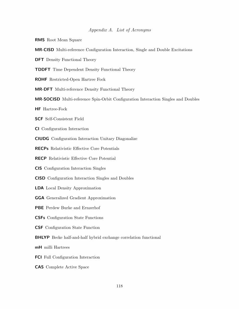
Appendix A. List of Acronyms
RMS Root Mean Square
MR-CISD Multi-reference Configuration Interaction, Single and Double Excitations
DFT Density Functional Theory
TDDFT Time Dependent Density Functional Theory
ROHF Restricted-Open Hartree Fock
MR-DFT Multi-reference Density Functional Theory
MR-SOCISD Multi-reference Spin-Orbit Configuration Interaction Singles and Doubles
HF Hartree-Fock
SCF Self-Consistent Field
CI Configuration Interaction
CIUDG Configuration Interaction Unitary Diagonalize
RECPs Relativistic Effective Core Potentials
RECP Relativistic Effective Core Potential
CIS Configuration Interaction Singles
CISD Configuration Interaction Singles and Doubles
LDA Local Density Approximation
GGA Generalized Gradient Approximation
PBE Perdew Burke and Ernzerhof
CSFs Configuration State Functions
CSF Configuration State Function
BHLYP Becke half-and-half hybrid exchange correlation functional
mH milli Hartrees
FCI Full Configuration Interaction
CAS Complete Active Space
118
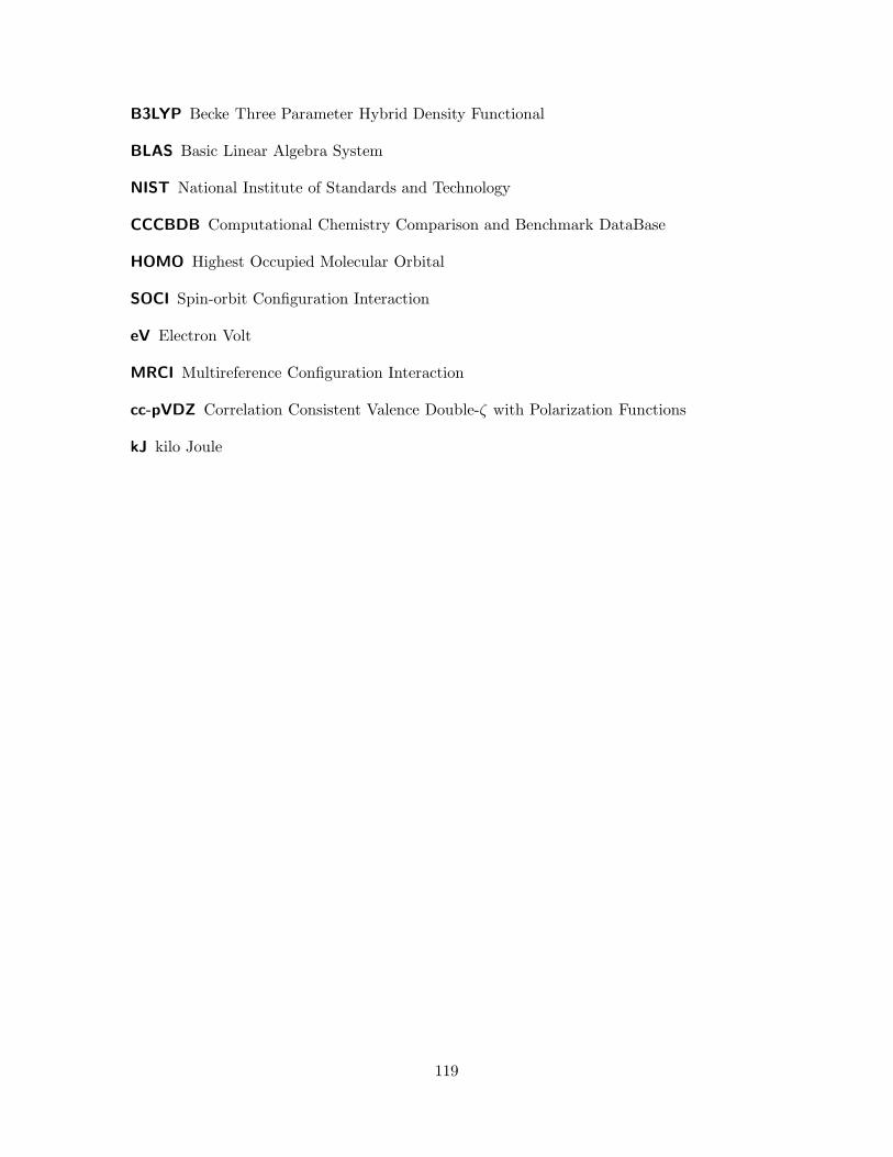
B3LYP Becke Three Parameter Hybrid Density Functional
BLAS Basic Linear Algebra System
NIST National Institute of Standards and Technology
CCCBDB Computational Chemistry Comparison and Benchmark DataBase
HOMO Highest Occupied Molecular Orbital
SOCI Spin-orbit Configuration Interaction
eV Electron Volt
MRCI Multireference Configuration Interaction
cc-pVDZ Correlation Consistent Valence Double-ζ with Polarization Functions
kJ kilo Joule
119

Appendix B. DFT/MRCI Damping Parameter Selection
This appendix contains the results of FCI calculations on the atomic and molecular systems
used to determine the optimal damping parameters used in the uranium calculations, as
well as DFT/MRCI calculations performed over a wide range of damping parameters, p1
and p2. All DFT/MRCI calculations were performed on a 20 by 20 grid in the damping
parameter space. Statistical analysis of the error between the electronic excitation energy
as computed by DFT/MRCI and FCI is also listed.
For each system examined, a density plot representing the absolute value of the error
between the DFT/MRCI and FCI for the lowest, spin-multiplicity allowed electronic transi-
tion. The range of the damping paramters in the density plots are 0 ≤ p1 ≤ 1, 0 ≤ p2 ≤ 10.
The squares of the Hartree-Fock configurations from ab initio calculations on each of
the systems is given in Table B. It is a measure of the multi-reference character of system.
Table 20 MR-CISD Hartree-Fock Configuration Coefficients For Systems Used for Damp-ing Parameter Determination
System Basis Set c20 State
H2 cc-pVDZ 0.983859 1Σ+g
H2 cc-pVTZ 0.985199 1Σ+g
He cc-pVDZ 0.992739 1S
He cc-pVTZ 0.992673 1S
Li, cc-pVDZ 0.999924 2S
Li, cc-pVTZ 0.999664 2S
Be cc-pVDZ 0.906694 1S
Be cc-pVTZ 0.904388 1S
B cc-pVDZ 0.928991 2P
C cc-pVDZ 0.951450 3P
N cc-pVDZ 0.969066 4S
O cc-pVDZ 0.967909 3P
F cc-pVDZ 0.970048 2P
Ne cc-pVDZ 0.972435 1S
Be2 cc-pVDZ 0.787166 1Σ+g
120

Hydrogen Molecule, cc-pVDZ Basis
The H2 cc-pVDZ calculation had 10 basis functions. The active space used in the
DFT/MRCI calculations for H2 was a CAS over the 1σ, and 2σ orbitals, with the four
highest energy virtual orbitals frozen.
Table 21 Hydrogen Molecule, cc-pVDZ Basis Set, Full CI Results
Eigenvalue Energy(au) Spin QuantumNumber(S)
1 -1.1634454317 0.002 -0.7719930623 1.003 -0.6526531835 0.004 -0.5172916288 1.005 -0.3771969905 0.006 -0.1712406269 1.007 -0.0860211873 0.008 -0.0260620923 0.009 0.0994560644 1.0010 0.0994560644 1.00
Table 22 DFT/MRCI Error Analysis for Hydrogen Molecule, cc-pVDZ Basis
p1 p2 Average Standard deviationerror (mH) of error (mH)
0 ≤ p1 ≤ 1 0 ≤ p2 ≤ 10 3.17379 1.43684
In figure 8, the horizontal axis is p1, the vertical axis is p2, and the absolute error
units are milli-Hartrees.
121
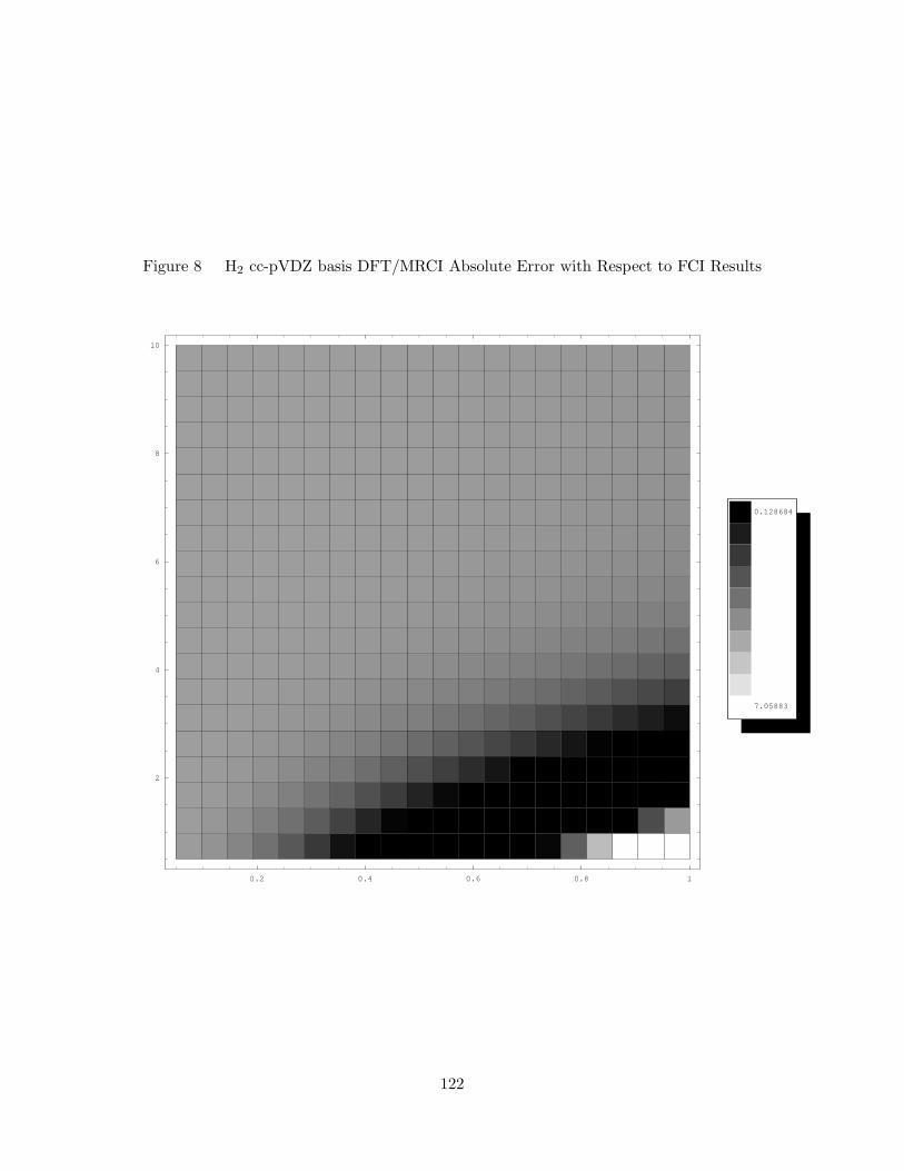
Figure 8 H2 cc-pVDZ basis DFT/MRCI Absolute Error with Respect to FCI Results
0.2 0.4 0.6 0.8 1
2
4
6
8
10
7.05883
0.128684
122
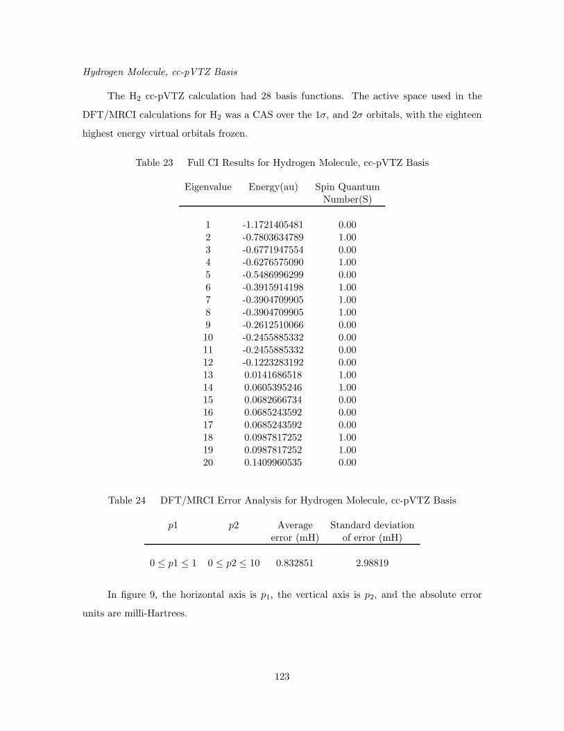
Hydrogen Molecule, cc-pVTZ Basis
The H2 cc-pVTZ calculation had 28 basis functions. The active space used in the
DFT/MRCI calculations for H2 was a CAS over the 1σ, and 2σ orbitals, with the eighteen
highest energy virtual orbitals frozen.
Table 23 Full CI Results for Hydrogen Molecule, cc-pVTZ Basis
Eigenvalue Energy(au) Spin QuantumNumber(S)
1 -1.1721405481 0.002 -0.7803634789 1.003 -0.6771947554 0.004 -0.6276575090 1.005 -0.5486996299 0.006 -0.3915914198 1.007 -0.3904709905 1.008 -0.3904709905 1.009 -0.2612510066 0.0010 -0.2455885332 0.0011 -0.2455885332 0.0012 -0.1223283192 0.0013 0.0141686518 1.0014 0.0605395246 1.0015 0.0682666734 0.0016 0.0685243592 0.0017 0.0685243592 0.0018 0.0987817252 1.0019 0.0987817252 1.0020 0.1409960535 0.00
Table 24 DFT/MRCI Error Analysis for Hydrogen Molecule, cc-pVTZ Basis
p1 p2 Average Standard deviationerror (mH) of error (mH)
0 ≤ p1 ≤ 1 0 ≤ p2 ≤ 10 0.832851 2.98819
In figure 9, the horizontal axis is p1, the vertical axis is p2, and the absolute error
units are milli-Hartrees.
123
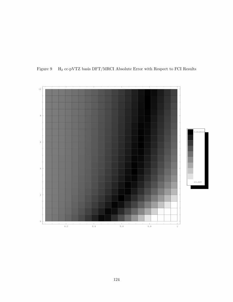
Figure 9 H2 cc-pVTZ basis DFT/MRCI Absolute Error with Respect to FCI Results
0.2 0.4 0.6 0.8 1
0
2
4
6
8
10
13.219
0.0125115
124
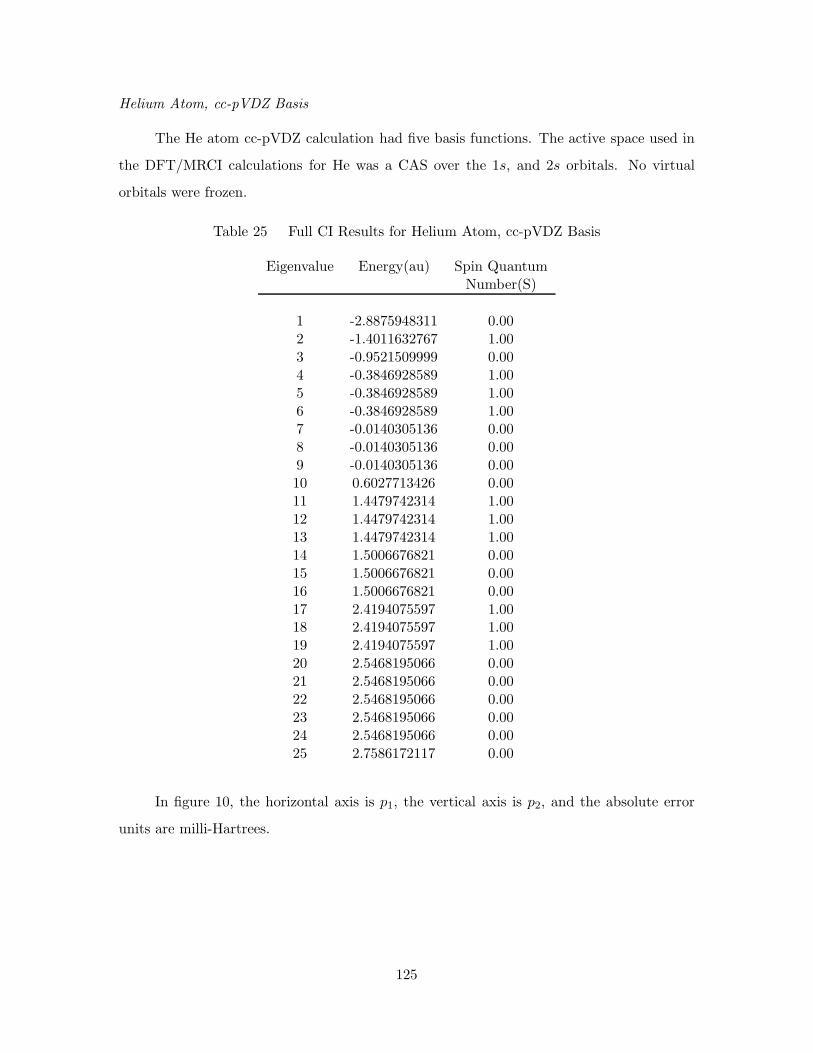
Helium Atom, cc-pVDZ Basis
The He atom cc-pVDZ calculation had five basis functions. The active space used in
the DFT/MRCI calculations for He was a CAS over the 1s, and 2s orbitals. No virtual
orbitals were frozen.
Table 25 Full CI Results for Helium Atom, cc-pVDZ Basis
Eigenvalue Energy(au) Spin QuantumNumber(S)
1 -2.8875948311 0.002 -1.4011632767 1.003 -0.9521509999 0.004 -0.3846928589 1.005 -0.3846928589 1.006 -0.3846928589 1.007 -0.0140305136 0.008 -0.0140305136 0.009 -0.0140305136 0.0010 0.6027713426 0.0011 1.4479742314 1.0012 1.4479742314 1.0013 1.4479742314 1.0014 1.5006676821 0.0015 1.5006676821 0.0016 1.5006676821 0.0017 2.4194075597 1.0018 2.4194075597 1.0019 2.4194075597 1.0020 2.5468195066 0.0021 2.5468195066 0.0022 2.5468195066 0.0023 2.5468195066 0.0024 2.5468195066 0.0025 2.7586172117 0.00
In figure 10, the horizontal axis is p1, the vertical axis is p2, and the absolute error
units are milli-Hartrees.
125
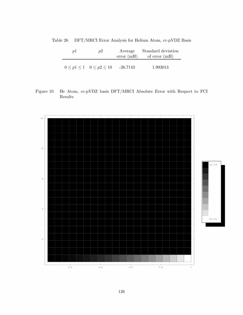
Table 26 DFT/MRCI Error Analysis for Helium Atom, cc-pVDZ Basis
p1 p2 Average Standard deviationerror (mH) of error (mH)
0 ≤ p1 ≤ 1 0 ≤ p2 ≤ 10 -26.7143 1.993013
Figure 10 He Atom, cc-pVDZ basis DFT/MRCI Absolute Error with Respect to FCIResults
0.2 0.4 0.6 0.8 1
2
4
6
8
10
26.733
26.714
126
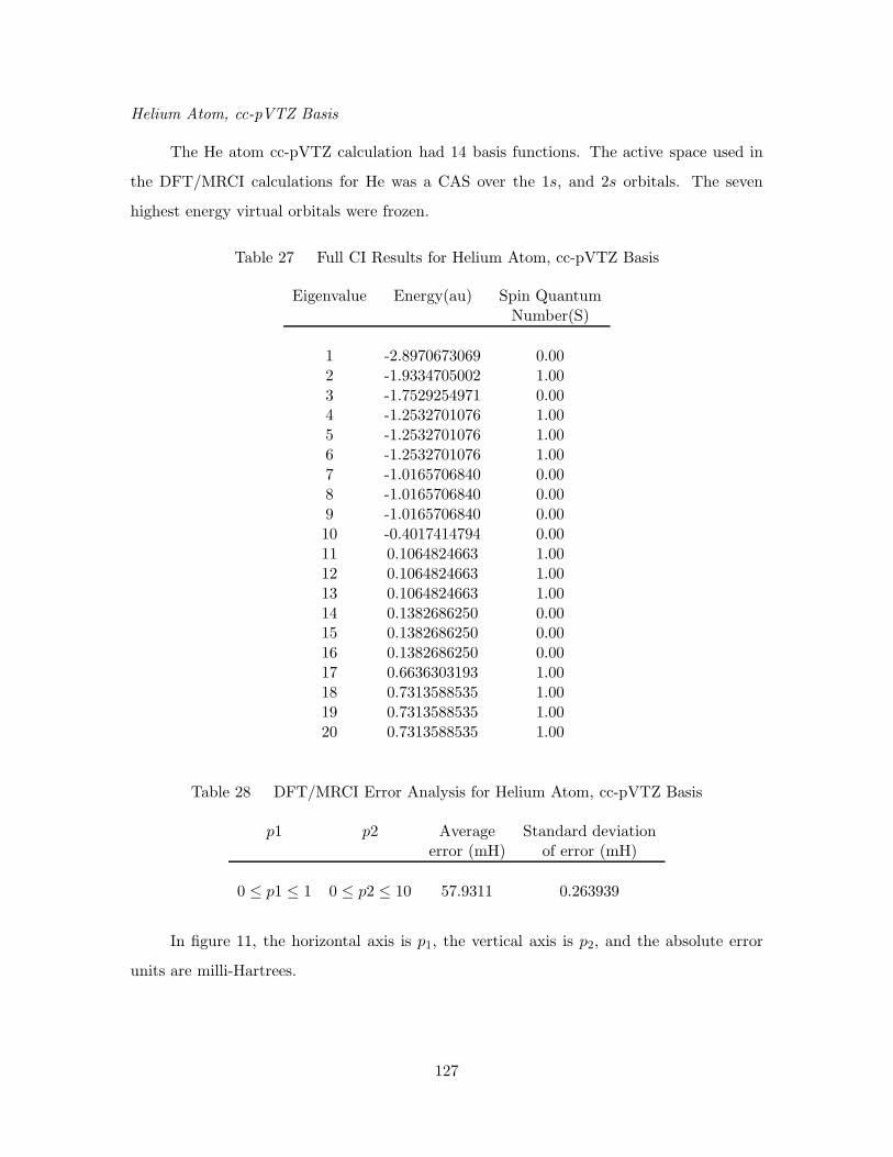
Helium Atom, cc-pVTZ Basis
The He atom cc-pVTZ calculation had 14 basis functions. The active space used in
the DFT/MRCI calculations for He was a CAS over the 1s, and 2s orbitals. The seven
highest energy virtual orbitals were frozen.
Table 27 Full CI Results for Helium Atom, cc-pVTZ Basis
Eigenvalue Energy(au) Spin QuantumNumber(S)
1 -2.8970673069 0.002 -1.9334705002 1.003 -1.7529254971 0.004 -1.2532701076 1.005 -1.2532701076 1.006 -1.2532701076 1.007 -1.0165706840 0.008 -1.0165706840 0.009 -1.0165706840 0.0010 -0.4017414794 0.0011 0.1064824663 1.0012 0.1064824663 1.0013 0.1064824663 1.0014 0.1382686250 0.0015 0.1382686250 0.0016 0.1382686250 0.0017 0.6636303193 1.0018 0.7313588535 1.0019 0.7313588535 1.0020 0.7313588535 1.00
Table 28 DFT/MRCI Error Analysis for Helium Atom, cc-pVTZ Basis
p1 p2 Average Standard deviationerror (mH) of error (mH)
0 ≤ p1 ≤ 1 0 ≤ p2 ≤ 10 57.9311 0.263939
In figure 11, the horizontal axis is p1, the vertical axis is p2, and the absolute error
units are milli-Hartrees.
127
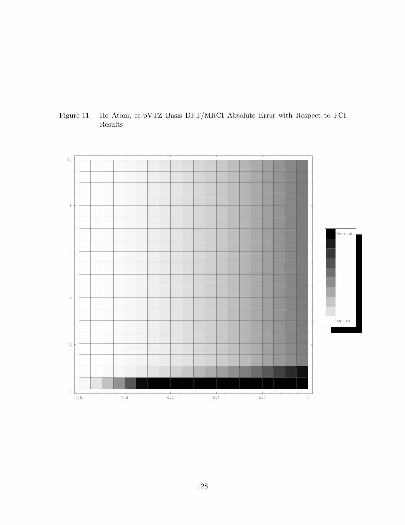
Figure 11 He Atom, cc-pVTZ Basis DFT/MRCI Absolute Error with Respect to FCIResults
0.5 0.6 0.7 0.8 0.9 1
0
2
4
6
8
10
58.0181
55.4338
128
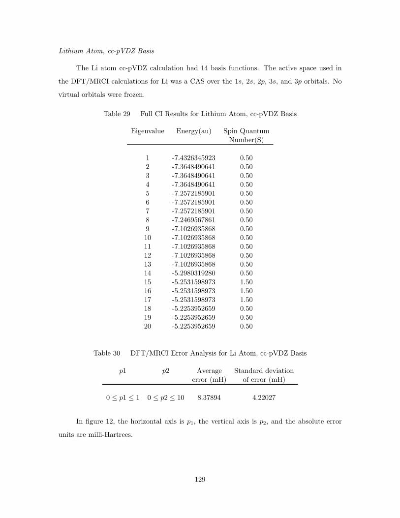
Lithium Atom, cc-pVDZ Basis
The Li atom cc-pVDZ calculation had 14 basis functions. The active space used in
the DFT/MRCI calculations for Li was a CAS over the 1s, 2s, 2p, 3s, and 3p orbitals. No
virtual orbitals were frozen.
Table 29 Full CI Results for Lithium Atom, cc-pVDZ Basis
Eigenvalue Energy(au) Spin QuantumNumber(S)
1 -7.4326345923 0.502 -7.3648490641 0.503 -7.3648490641 0.504 -7.3648490641 0.505 -7.2572185901 0.506 -7.2572185901 0.507 -7.2572185901 0.508 -7.2469567861 0.509 -7.1026935868 0.5010 -7.1026935868 0.5011 -7.1026935868 0.5012 -7.1026935868 0.5013 -7.1026935868 0.5014 -5.2980319280 0.5015 -5.2531598973 1.5016 -5.2531598973 1.5017 -5.2531598973 1.5018 -5.2253952659 0.5019 -5.2253952659 0.5020 -5.2253952659 0.50
Table 30 DFT/MRCI Error Analysis for Li Atom, cc-pVDZ Basis
p1 p2 Average Standard deviationerror (mH) of error (mH)
0 ≤ p1 ≤ 1 0 ≤ p2 ≤ 10 8.37894 4.22027
In figure 12, the horizontal axis is p1, the vertical axis is p2, and the absolute error
units are milli-Hartrees.
129
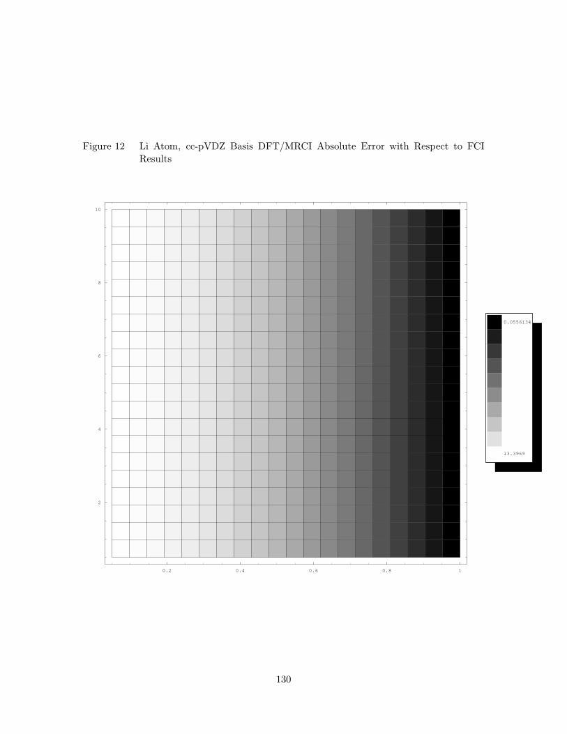
Figure 12 Li Atom, cc-pVDZ Basis DFT/MRCI Absolute Error with Respect to FCIResults
0.2 0.4 0.6 0.8 1
2
4
6
8
10
13.3969
0.0556134
130

Lithium Atom, cc-pVTZ Basis
The Li atom cc-pVTZ calculation had 30 basis functions. The active space used in
the DFT/MRCI calculations for Li was a CAS over the 1s, 2s, 2p, 3s, and 3p orbitals. The
highest energy virtual orbital was frozen. ROHF open-shell coefficients corresponding to
the high-spin 2S state were used to generate the initial orbitals, with exchange-correlation
potential integrals from an unrestricted DFT calculation.
Table 31 Full CI Results for Lithium Atom, cc-pVTZ Basis
Eigenvalue Energy(au) Spin QuantumNumber(S)
1 -7.4332546271 0.502 -7.3654330817 0.503 -7.3654330817 0.504 -7.3654330817 0.505 -7.2827258411 0.506 -7.2761519403 0.507 -7.2761519403 0.508 -7.2761519403 0.509 -7.2021446003 0.5010 -7.2021446003 0.5011 -7.2021446003 0.5012 -7.2021446003 0.5013 -7.2021446003 0.5014 -7.0789295728 0.5015 -7.0789295728 0.5016 -7.0789295728 0.5017 -7.0370981897 0.5018 -6.7539585204 0.5019 -6.7539585204 0.5020 -6.7539585204 0.5021 -6.7539585204 0.5022 -6.7539585204 0.5023 -6.7260996854 0.5024 -6.7260996854 0.5025 -6.7260996854 0.5026 -6.7260996854 0.5027 -6.7260996854 0.5028 -6.7260996854 0.5029 -6.7260996854 0.5030 -5.3317686889 0.50
131

Table 32 DFT/MRCI Error Analysis for Li Atom, cc-pVTZ Basis
p1 p2 Average Standard deviationerror (mH) of error (mH)
0 ≤ p1 ≤ 1 0 ≤ p2 ≤ 10 12.2333 5.61206
132

In figure 13, the horizontal axis is p1, the vertical axis is p2, and the absolute error
units are milli-Hartrees.
Figure 13 Li Atom, cc-pVTZ Basis DFT/MRCI Absolute Error with Respect to FCIResults
0.2 0.4 0.6 0.8 1
2
4
6
8
10
19.0837
1.42195
133
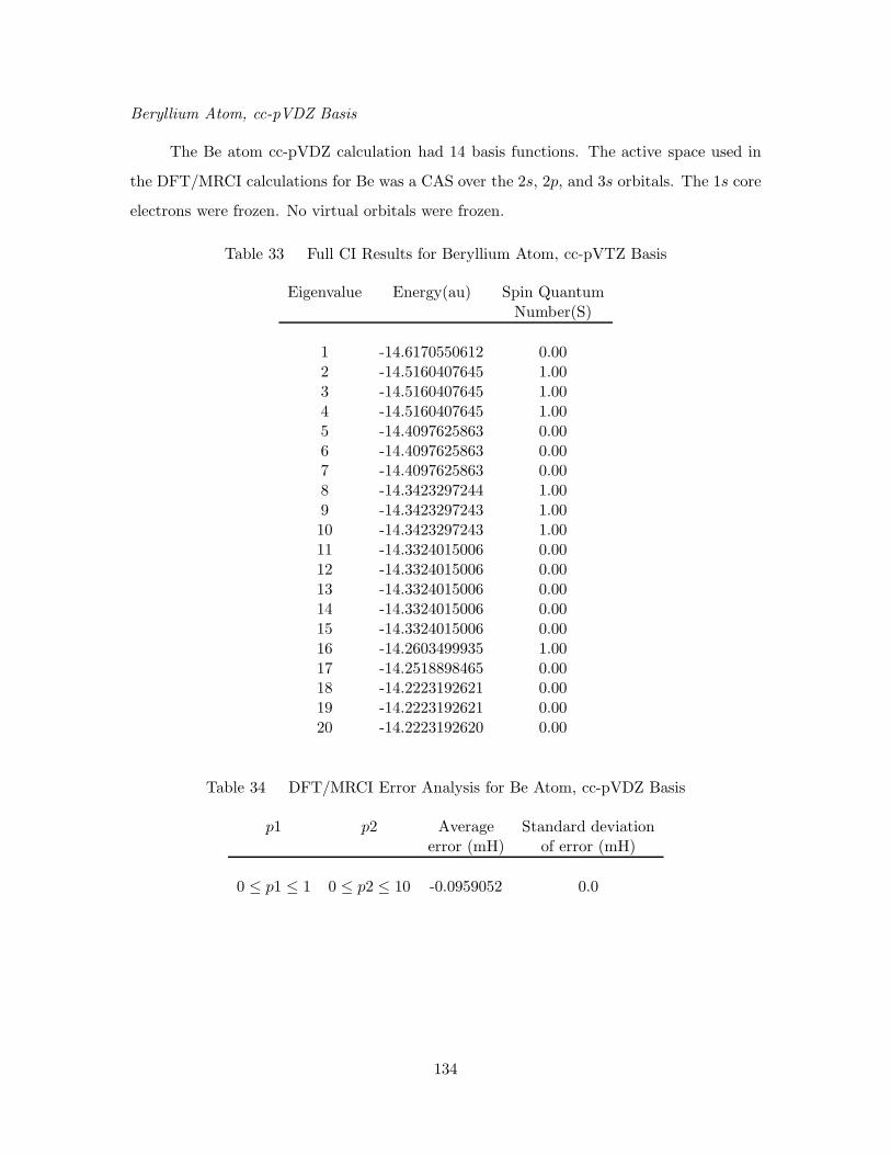
Beryllium Atom, cc-pVDZ Basis
The Be atom cc-pVDZ calculation had 14 basis functions. The active space used in
the DFT/MRCI calculations for Be was a CAS over the 2s, 2p, and 3s orbitals. The 1s core
electrons were frozen. No virtual orbitals were frozen.
Table 33 Full CI Results for Beryllium Atom, cc-pVTZ Basis
Eigenvalue Energy(au) Spin QuantumNumber(S)
1 -14.6170550612 0.002 -14.5160407645 1.003 -14.5160407645 1.004 -14.5160407645 1.005 -14.4097625863 0.006 -14.4097625863 0.007 -14.4097625863 0.008 -14.3423297244 1.009 -14.3423297243 1.0010 -14.3423297243 1.0011 -14.3324015006 0.0012 -14.3324015006 0.0013 -14.3324015006 0.0014 -14.3324015006 0.0015 -14.3324015006 0.0016 -14.2603499935 1.0017 -14.2518898465 0.0018 -14.2223192621 0.0019 -14.2223192621 0.0020 -14.2223192620 0.00
Table 34 DFT/MRCI Error Analysis for Be Atom, cc-pVDZ Basis
p1 p2 Average Standard deviationerror (mH) of error (mH)
0 ≤ p1 ≤ 1 0 ≤ p2 ≤ 10 -0.0959052 0.0
134
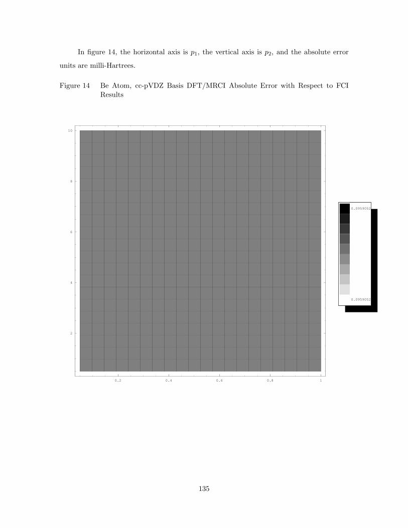
In figure 14, the horizontal axis is p1, the vertical axis is p2, and the absolute error
units are milli-Hartrees.
Figure 14 Be Atom, cc-pVDZ Basis DFT/MRCI Absolute Error with Respect to FCIResults
0.2 0.4 0.6 0.8 1
2
4
6
8
10
0.0959052
0.0959052
135
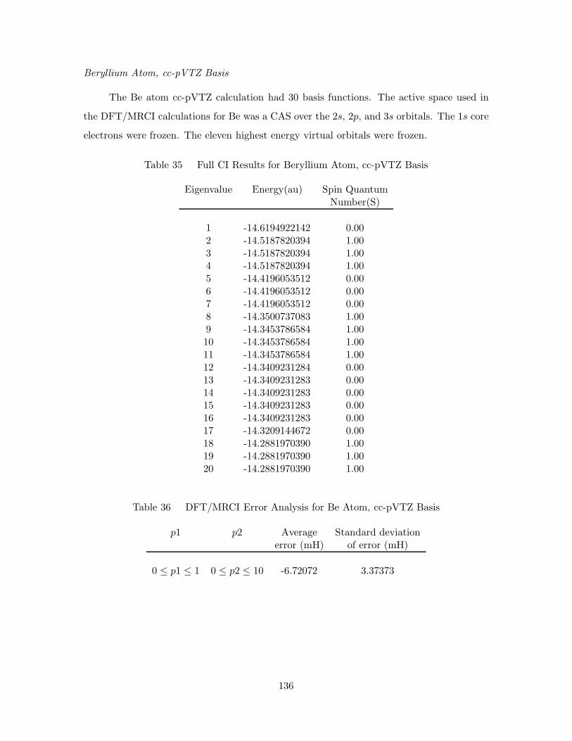
Beryllium Atom, cc-pVTZ Basis
The Be atom cc-pVTZ calculation had 30 basis functions. The active space used in
the DFT/MRCI calculations for Be was a CAS over the 2s, 2p, and 3s orbitals. The 1s core
electrons were frozen. The eleven highest energy virtual orbitals were frozen.
Table 35 Full CI Results for Beryllium Atom, cc-pVTZ Basis
Eigenvalue Energy(au) Spin QuantumNumber(S)
1 -14.6194922142 0.002 -14.5187820394 1.003 -14.5187820394 1.004 -14.5187820394 1.005 -14.4196053512 0.006 -14.4196053512 0.007 -14.4196053512 0.008 -14.3500737083 1.009 -14.3453786584 1.0010 -14.3453786584 1.0011 -14.3453786584 1.0012 -14.3409231284 0.0013 -14.3409231283 0.0014 -14.3409231283 0.0015 -14.3409231283 0.0016 -14.3409231283 0.0017 -14.3209144672 0.0018 -14.2881970390 1.0019 -14.2881970390 1.0020 -14.2881970390 1.00
Table 36 DFT/MRCI Error Analysis for Be Atom, cc-pVTZ Basis
p1 p2 Average Standard deviationerror (mH) of error (mH)
0 ≤ p1 ≤ 1 0 ≤ p2 ≤ 10 -6.72072 3.37373
136

In figure 15, the horizontal axis is p1, the vertical axis is p2, and the absolute error
units are milli-Hartrees.
Figure 15 Be Atom, cc-pVTZ Basis DFT/MRCI Absolute Error with Respect to FCIResults
0.2 0.4 0.6 0.8 1
2
4
6
8
10
10.1144
0.0182426
Boron Atom, cc-pVDZ Basis
The B atom cc-pVDZ calculation had 14 basis functions. The active space used in
the DFT/MRCI calculations for B was a CAS over the 2s, 2p, 3s, and 3p orbitals. The 1s
137
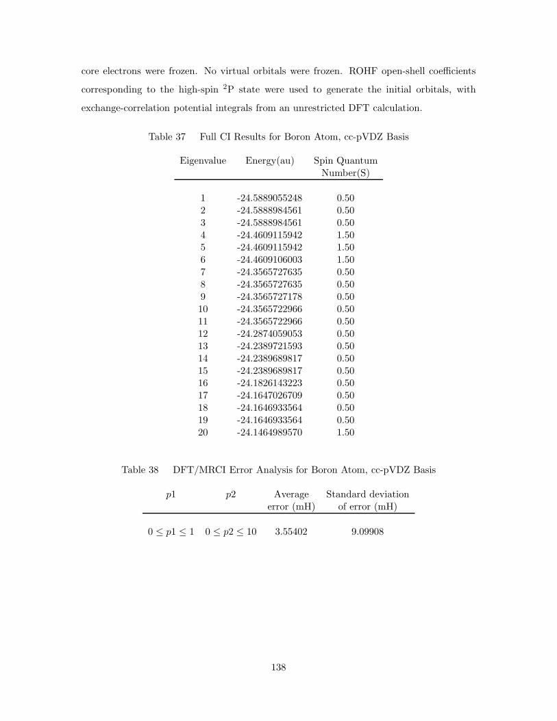
core electrons were frozen. No virtual orbitals were frozen. ROHF open-shell coefficients
corresponding to the high-spin 2P state were used to generate the initial orbitals, with
exchange-correlation potential integrals from an unrestricted DFT calculation.
Table 37 Full CI Results for Boron Atom, cc-pVDZ Basis
Eigenvalue Energy(au) Spin QuantumNumber(S)
1 -24.5889055248 0.502 -24.5888984561 0.503 -24.5888984561 0.504 -24.4609115942 1.505 -24.4609115942 1.506 -24.4609106003 1.507 -24.3565727635 0.508 -24.3565727635 0.509 -24.3565727178 0.5010 -24.3565722966 0.5011 -24.3565722966 0.5012 -24.2874059053 0.5013 -24.2389721593 0.5014 -24.2389689817 0.5015 -24.2389689817 0.5016 -24.1826143223 0.5017 -24.1647026709 0.5018 -24.1646933564 0.5019 -24.1646933564 0.5020 -24.1464989570 1.50
Table 38 DFT/MRCI Error Analysis for Boron Atom, cc-pVDZ Basis
p1 p2 Average Standard deviationerror (mH) of error (mH)
0 ≤ p1 ≤ 1 0 ≤ p2 ≤ 10 3.55402 9.09908
138

In figure 16, the horizontal axis is p1, the vertical axis is p2, and the absolute error
units are milli-Hartrees.
Figure 16 B Atom, cc-pVDZ Basis DFT/MRCI Absolute Error with Respect to FCIResults
0.2 0.4 0.6 0.8 1
2
4
6
8
10
18.0833
0.00837789
139
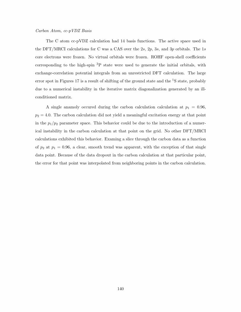
Carbon Atom, cc-pVDZ Basis
The C atom cc-pVDZ calculation had 14 basis functions. The active space used in
the DFT/MRCI calculations for C was a CAS over the 2s, 2p, 3s, and 3p orbitals. The 1s
core electrons were frozen. No virtual orbitals were frozen. ROHF open-shell coefficients
corresponding to the high-spin 3P state were used to generate the initial orbitals, with
exchange-correlation potential integrals from an unrestricted DFT calculation. The large
error spot in Figures 17 is a result of shifting of the ground state and the 1S state, probably
due to a numerical instability in the iterative matrix diagonalization generated by an ill-
conditioned matrix.
A single anamoly occured during the carbon calculation calculation at p1 = 0.96,
p2 = 4.0. The carbon calculation did not yield a meaningful excitation energy at that point
in the p1/p2 parameter space. This behavior could be due to the introduction of a numer-
ical instability in the carbon calculation at that point on the grid. No other DFT/MRCI
calculations exhibited this behavior. Examing a slice through the carbon data as a function
of p2 at p1 = 0.96, a clear, smooth trend was apparent, with the exception of that single
data point. Because of the data dropout in the carbon calculation at that particular point,
the error for that point was interpolated from neighboring points in the carbon calculation.
140
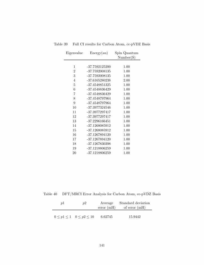
Table 39 Full CI results for Carbon Atom, cc-pVDZ Basis
Eigenvalue Energy(au) Spin QuantumNumber(S)
1 -37.7592125200 1.002 -37.7592008135 1.003 -37.7592008135 1.004 -37.6165280238 2.005 -37.4548851325 1.006 -37.4548836429 1.007 -37.4548836429 1.008 -37.4548797964 1.009 -37.4548797964 1.0010 -37.3977324546 1.0011 -37.3977297417 1.0012 -37.3977297417 1.0013 -37.2296166451 1.0014 -37.1268085912 1.0015 -37.1268085912 1.0016 -37.1267894120 1.0017 -37.1267894120 1.0018 -37.1267830398 1.0019 -37.1218806259 1.0020 -37.1218806259 1.00
Table 40 DFT/MRCI Error Analysis for Carbon Atom, cc-pVDZ Basis
p1 p2 Average Standard deviationerror (mH) of error (mH)
0 ≤ p1 ≤ 1 0 ≤ p2 ≤ 10 6.62745 15.9442
141
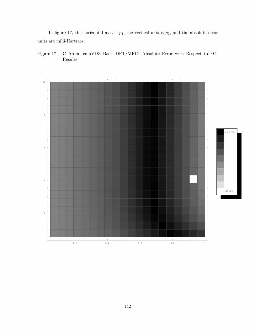
In figure 17, the horizontal axis is p1, the vertical axis is p2, and the absolute error
units are milli-Hartrees.
Figure 17 C Atom, cc-pVDZ Basis DFT/MRCI Absolute Error with Respect to FCIResults
0.2 0.4 0.6 0.8 1
2
4
6
8
10
195.66
0.023729
142
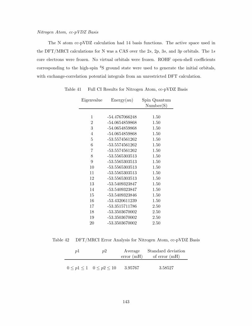
Nitrogen Atom, cc-pVDZ Basis
The N atom cc-pVDZ calculation had 14 basis functions. The active space used in
the DFT/MRCI calculations for N was a CAS over the 2s, 2p, 3s, and 3p orbitals. The 1s
core electrons were frozen. No virtual orbitals were frozen. ROHF open-shell coefficients
corresponding to the high-spin 4S ground state were used to generate the initial orbitals,
with exchange-correlation potential integrals from an unrestricted DFT calculation.
Table 41 Full CI Results for Nitrogen Atom, cc-pVDZ Basis
Eigenvalue Energy(au) Spin QuantumNumber(S)
1 -54.4767066248 1.502 -54.0654859868 1.503 -54.0654859868 1.504 -54.0654859868 1.505 -53.5574561262 1.506 -53.5574561262 1.507 -53.5574561262 1.508 -53.5565303513 1.509 -53.5565303513 1.5010 -53.5565303513 1.5011 -53.5565303513 1.5012 -53.5565303513 1.5013 -53.5409323847 1.5014 -53.5409323847 1.5015 -53.5409323846 1.5016 -53.4320611239 1.5017 -53.3515711786 2.5018 -53.3503670002 2.5019 -53.3503670002 2.5020 -53.3503670002 2.50
Table 42 DFT/MRCI Error Analysis for Nitrogen Atom, cc-pVDZ Basis
p1 p2 Average Standard deviationerror (mH) of error (mH)
0 ≤ p1 ≤ 1 0 ≤ p2 ≤ 10 3.95767 3.58527
143

In figure 18, the horizontal axis is p1, the vertical axis is p2, and the absolute error
units are milli-Hartrees.
144
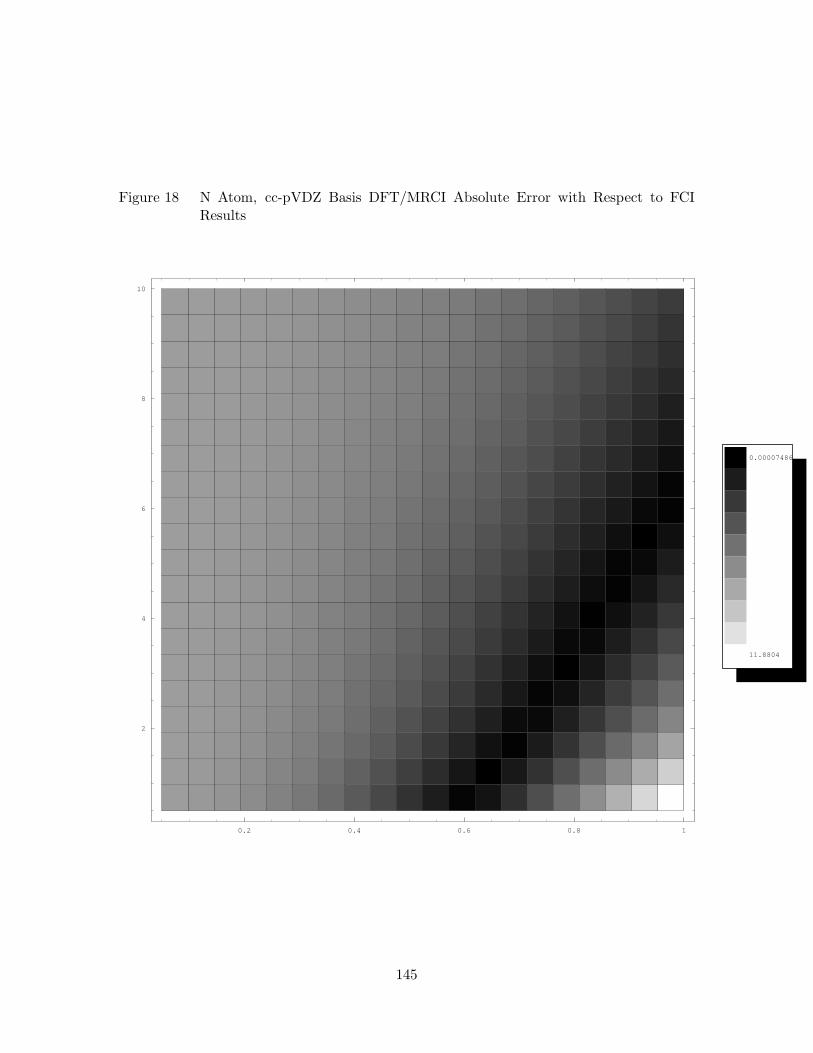
Figure 18 N Atom, cc-pVDZ Basis DFT/MRCI Absolute Error with Respect to FCIResults
0.2 0.4 0.6 0.8 1
2
4
6
8
10
11.8804
0.0000748667
145

Oxygen atom, cc-pVDZ Basis set
The O atom cc-pVDZ calculation had 14 basis functions. The active space used in
the DFT/MRCI calculations for N was a CAS over the 2s, 2p, 3s, and 3p orbitals. The 1s
core electrons were frozen. No virtual orbitals were frozen. ROHF open-shell coefficients
corresponding to the high-spin 3P ground state were used to generate the initial orbitals,
with exchange-correlation potential integrals from an unrestricted DFT calculation.
Table 43 Full CI Results for Oxygen Atom, cc-pVDZ Basis
Eigenvalue Energy(au) Spin QuantumNumber(S)
1 -74.9076668782 1.002 -74.9076668782 1.003 -74.9076651533 1.004 -74.3144151907 1.005 -74.3144151907 1.006 -74.3144089572 1.007 -73.8961915673 2.008 -73.8961707443 2.009 -73.8961707443 2.0010 -73.8294403260 1.0011 -73.8294047725 1.0012 -73.8294047725 1.0013 -73.8197705793 2.0014 -73.7854164706 1.0015 -73.7854164706 1.0016 -73.7853895151 1.0017 -73.7853895151 1.0018 -73.7853815338 1.0019 -73.7301128656 1.0020 -73.7301128656 1.0021 -73.7301004221 1.0022 -73.7301004221 1.0023 -73.7300923622 1.0024 -73.7300923622 1.0025 -73.7296367317 1.00
146

Table 44 DFT/MRCI Error Analysis for Oxygen Atom, cc-pVDZ Basis
p1 p2 Average Standard deviationerror (mH) of error (mH)
0 ≤ p1 ≤ 1 0 ≤ p2 ≤ 10 37.497 2.42638
147

In figure 19, the horizontal axis is p1, the vertical axis is p2, and the absolute error
units are milli-Hartrees.
Figure 19 O Atom, cc-pVDZ Basis DFT/MRCI Absolute Error with Respect to FCIResults
0.2 0.4 0.6 0.8 1
2
4
6
8
10
38.4897
18.998
148

Fluorine Atom, cc-pVDZ Basis
The F atom cc-pVDZ calculation had 14 basis functions. The active space used in
the DFT/MRCI calculations for F was a CAS over the 2s, 2p, 3s, and 3p orbitals. The 1s
core electrons were frozen. No virtual orbitals were frozen. ROHF open-shell coefficients
corresponding to the high-spin 2P ground state were used to generate the initial orbitals,
with exchange-correlation potential integrals from an unrestricted DFT calculation.
Table 45 Full CI Results for Fluorine Atom, cc-pVDZ Basis
Eigenvalue Energy(au) Spin QuantumNumber(S)
1 -99.5250149572 0.502 -99.5250122692 0.503 -99.5250122692 0.504 -98.7098466484 0.505 -98.2263496364 1.506 -98.2263398709 1.507 -98.2263398709 1.508 -98.1722681950 0.509 -98.1722404883 0.5010 -98.1722404883 0.5011 -98.1452591018 1.5012 -98.1452591018 1.5013 -98.1452580440 1.5014 -98.1452580440 1.50
Table 46 DFT/MRCI Error Analysis for Fluorine Atom, cc-pVDZ Basis
p1 p2 Average Standard deviationerror (mH) of error (mH)
0 ≤ p1 ≤ 1 0 ≤ p2 ≤ 10 70.365 0.763109
149
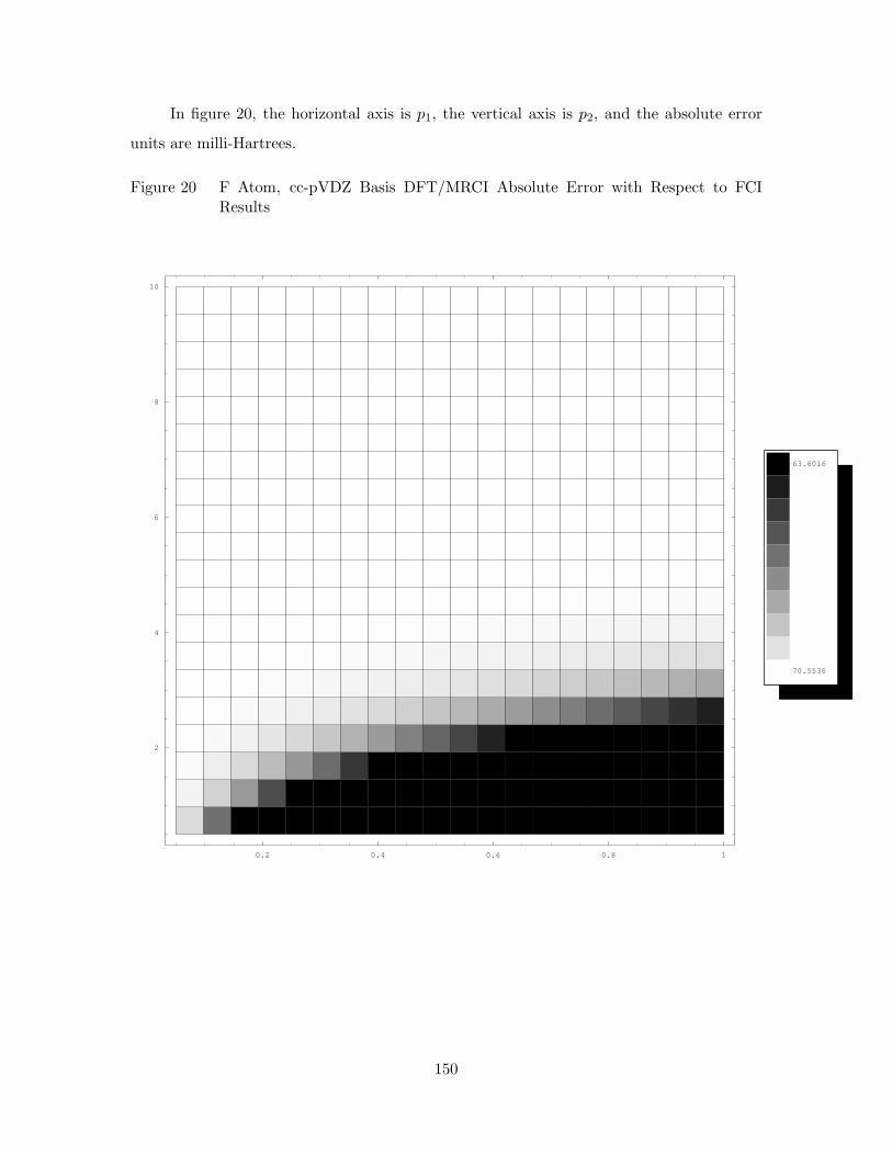
In figure 20, the horizontal axis is p1, the vertical axis is p2, and the absolute error
units are milli-Hartrees.
Figure 20 F Atom, cc-pVDZ Basis DFT/MRCI Absolute Error with Respect to FCIResults
0.2 0.4 0.6 0.8 1
2
4
6
8
10
70.5536
63.6016
150

Neon Atom, cc-pVDZ Basis
The Ne atom cc-pVDZ calculation had 14 basis functions. The active space used in
the DFT/MRCI calculations for Ne was a CAS over the 2s, 2p, 3s, and 3p orbitals. The 1s
core electrons were frozen. No virtual orbitals were frozen.
Table 47 Full CI Results for Neon Atom, cc-pVDZ Basis
Eigenvalue Energy(au) Spin QuantumNumber(S)
1 -128.6762641527 0.002 -127.0362874267 1.003 -126.9067374859 1.004 -126.9067374858 1.005 -126.9067374858 1.006 -126.9067374857 1.007 -126.9067374856 1.008 -126.8392428164 0.009 -126.8392428082 0.0010 -126.8392428052 0.0011 -126.8379777691 1.0012 -126.8379777659 1.0013 -126.8379777577 1.0014 -126.8208198490 0.00
Table 48 DFT/MRCI Error Analysis for Neon Atom, cc-pVDZ Basis
p1 p2 Average Standard deviationerror (mH) of error (mH)
0 ≤ p1 ≤ 1 0 ≤ p2 ≤ 10 33.3121 2.45285
151
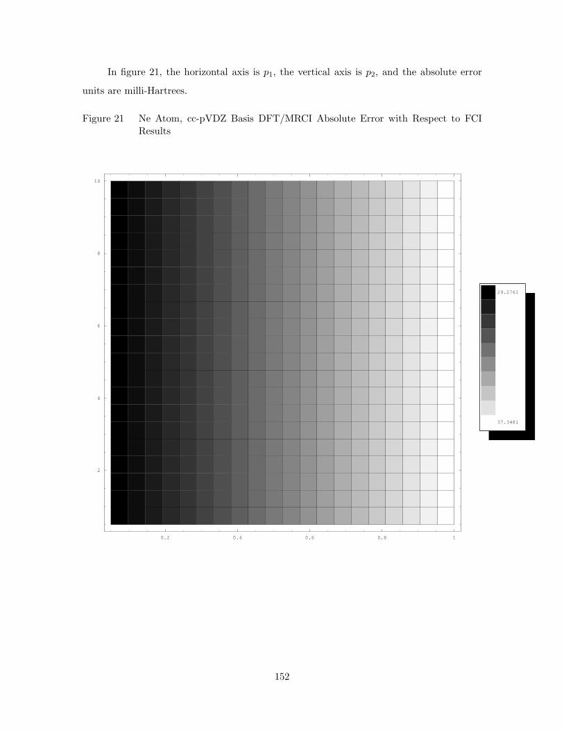
In figure 21, the horizontal axis is p1, the vertical axis is p2, and the absolute error
units are milli-Hartrees.
Figure 21 Ne Atom, cc-pVDZ Basis DFT/MRCI Absolute Error with Respect to FCIResults
0.2 0.4 0.6 0.8 1
2
4
6
8
10
37.3481
29.2761
152

Beryllium Dimer, cc-pVDZ Basis
The Be dimer cc-pVDZ calculation had 28 basis functions. The active space used in
the DFT/MRCI calculations for Be2 was a CAS over the 2σ, 1π, 1π∗, 2σ∗, 3σ and 3σ∗
orbitals. The 1σ and 1σ∗ orbitals were frozen.
Table 49 Full CI Results for Beryllium Dimer, cc-pVDZ Basis
Eigenvalue Energy(au) Spin QuantumNumber(S)
1 -29.2338409859 0.002 -29.1914009165 1.003 -29.1802291199 1.004 -29.1802291199 1.005 -29.1476359431 0.006 -29.1476359431 0.007 -29.1225304798 1.008 -29.1225304798 1.009 -29.1156678694 0.0010 -29.1156678694 0.0011 -29.1143923436 1.0012 -29.1143923436 1.0013 -29.1007032177 0.0014 -29.0976158970 1.0015 -29.0931147426 0.0016 -29.0868631904 0.0017 -29.0868631903 0.0018 -29.0828377548 2.0019 -29.0828377548 2.0020 -29.0769245880 1.0021 -29.0744258409 2.0022 -29.0666929750 0.0023 -29.0579750627 0.0024 -29.0578158780 1.0025 -29.0578158779 1.0026 -29.0534236925 1.0027 -29.0534236924 1.00
153

Table 50 DFT/MRCI Error Analysis for Beryllium Dimer, cc-pVDZ Basis
p1 p2 Average Standard deviationerror (mH) of error (mH)
0 ≤ p1 ≤ 1 0 ≤ p2 ≤ 10 -68.4936 3.41014
154
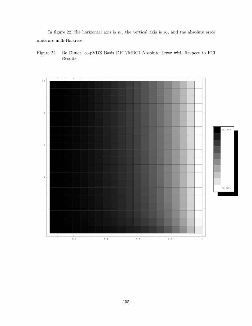
In figure 22, the horizontal axis is p1, the vertical axis is p2, and the absolute error
units are milli-Hartrees.
Figure 22 Be Dimer, cc-pVDZ Basis DFT/MRCI Absolute Error with Respect to FCIResults
0.2 0.4 0.6 0.8 1
2
4
6
8
10
76.9151
65.1056
155
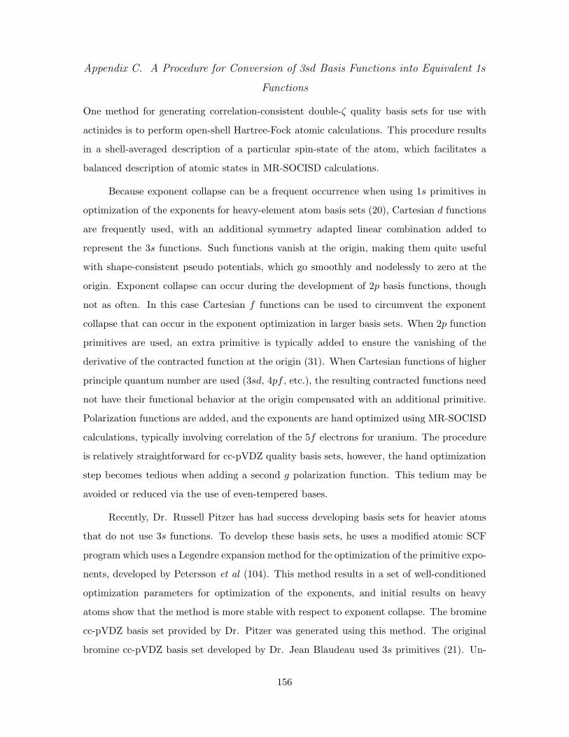
Appendix C. A Procedure for Conversion of 3sd Basis Functions into Equivalent 1s
Functions
One method for generating correlation-consistent double-ζ quality basis sets for use with
actinides is to perform open-shell Hartree-Fock atomic calculations. This procedure results
in a shell-averaged description of a particular spin-state of the atom, which facilitates a
balanced description of atomic states in MR-SOCISD calculations.
Because exponent collapse can be a frequent occurrence when using 1s primitives in
optimization of the exponents for heavy-element atom basis sets (20), Cartesian d functions
are frequently used, with an additional symmetry adapted linear combination added to
represent the 3s functions. Such functions vanish at the origin, making them quite useful
with shape-consistent pseudo potentials, which go smoothly and nodelessly to zero at the
origin. Exponent collapse can occur during the development of 2p basis functions, though
not as often. In this case Cartesian f functions can be used to circumvent the exponent
collapse that can occur in the exponent optimization in larger basis sets. When 2p function
primitives are used, an extra primitive is typically added to ensure the vanishing of the
derivative of the contracted function at the origin (31). When Cartesian functions of higher
principle quantum number are used (3sd, 4pf , etc.), the resulting contracted functions need
not have their functional behavior at the origin compensated with an additional primitive.
Polarization functions are added, and the exponents are hand optimized using MR-SOCISD
calculations, typically involving correlation of the 5f electrons for uranium. The procedure
is relatively straightforward for cc-pVDZ quality basis sets, however, the hand optimization
step becomes tedious when adding a second g polarization function. This tedium may be
avoided or reduced via the use of even-tempered bases.
Recently, Dr. Russell Pitzer has had success developing basis sets for heavier atoms
that do not use 3s functions. To develop these basis sets, he uses a modified atomic SCF
program which uses a Legendre expansion method for the optimization of the primitive expo-
nents, developed by Petersson et al (104). This method results in a set of well-conditioned
optimization parameters for optimization of the exponents, and initial results on heavy
atoms show that the method is more stable with respect to exponent collapse. The bromine
cc-pVDZ basis set provided by Dr. Pitzer was generated using this method. The original
bromine cc-pVDZ basis set developed by Dr. Jean Blaudeau used 3s primitives (21). Un-
156
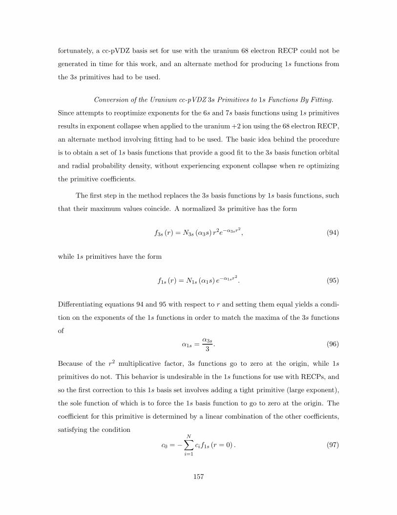
fortunately, a cc-pVDZ basis set for use with the uranium 68 electron RECP could not be
generated in time for this work, and an alternate method for producing 1s functions from
the 3s primitives had to be used.
Conversion of the Uranium cc-pVDZ 3s Primitives to 1s Functions By Fitting.
Since attempts to reoptimize exponents for the 6s and 7s basis functions using 1s primitives
results in exponent collapse when applied to the uranium +2 ion using the 68 electron RECP,
an alternate method involving fitting had to be used. The basic idea behind the procedure
is to obtain a set of 1s basis functions that provide a good fit to the 3s basis function orbital
and radial probability density, without experiencing exponent collapse when re optimizing
the primitive coefficients.
The first step in the method replaces the 3s basis functions by 1s basis functions, such
that their maximum values coincide. A normalized 3s primitive has the form
f3s (r) = N3s (α3s) r2e−α3sr2
, (94)
while 1s primitives have the form
f1s (r) = N1s (α1s) e−α1sr2
. (95)
Differentiating equations 94 and 95 with respect to r and setting them equal yields a condi-
tion on the exponents of the 1s functions in order to match the maxima of the 3s functions
of
α1s =α3s
3. (96)
Because of the r2 multiplicative factor, 3s functions go to zero at the origin, while 1s
primitives do not. This behavior is undesirable in the 1s functions for use with RECPs, and
so the first correction to this 1s basis set involves adding a tight primitive (large exponent),
the sole function of which is to force the 1s basis function to go to zero at the origin. The
coefficient for this primitive is determined by a linear combination of the other coefficients,
satisfying the condition
c0 = −N∑
i=1
cif1s (r = 0) . (97)
157

Now that the initial set of 1s primitives has been defined by the exponent condition in
equation 96 and the coefficient of the tight, canceling primitive has been determined, the
conversion procedure proceeds as follows:
1. Add another 1s primitive.
2. Reoptimize all 1s coefficients in an atomic SCF calculation.
3. Determine the coefficient on c0 from Equation 97.
4. Plot the difference in radial probability densities between the new 1s and original 3s
basis function.
This procedure is repeated until a decent fit occurs, or adding an additional 1s function
results in exponent collapse. The later case is typically the stopping point of the procedure.
Figure 23 shows the original 3s orbital along with the converted 1s orbital formed using
10 primitives from the above procedure. Figure 24 shows the radial probability density
functions of the original 3s orbital and the converted 1s orbital. Figure 25 shows the
difference between the radial probability densities of the original 3s and converted 1s basis
function.
Two figures of merit which measure the goodness of the fit procedure are defined for the
basis set conversion. Each value measures the average deviation in the radial probability
density between the original 3s function and the new 1s function over a range of radial
values. The average integrated density difference is defined as
AIDD =1
b− a
∫ b
a
(
r2 (φ∗3s (r)φ3s (r) − φ∗1s (r)φ1s (r)))
dr, (98)
while the average integrated absolute density difference is defined by
AIADD =1
b− a
∫ b
a
(
r2 |φ∗3s (r)φ3s (r) − φ∗1s (r)φ1s (r)|)
dr. (99)
The conversion procedure necessarily results in a smaller basis set than results from using
3sd functions. For every 3sd contraction, there are six symmetry adapted basis functions.
These correspond to the x2 + y2 + z2, which is the 3s function, and another five functions
representing 3d functions. For example, the original 3s basis had four contractions. This
158
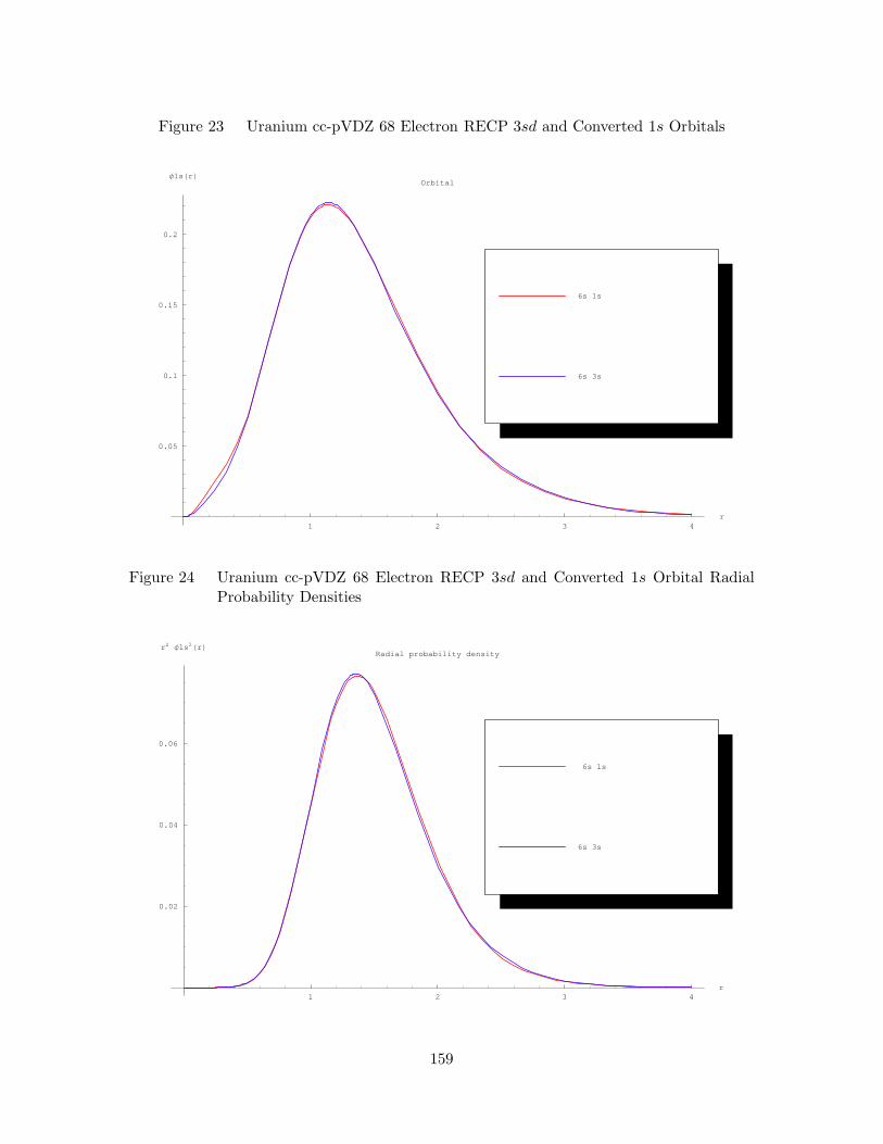
Figure 23 Uranium cc-pVDZ 68 Electron RECP 3sd and Converted 1s Orbitals
1 2 3 4r
0.05
0.1
0.15
0.2
Φ1sHrLOrbital
6s 3s
6s 1s
Figure 24 Uranium cc-pVDZ 68 Electron RECP 3sd and Converted 1s Orbital RadialProbability Densities
1 2 3 4r
0.02
0.04
0.06
r2 Φ1s2HrLRadial probability density
6s 3s
6s 1s
159
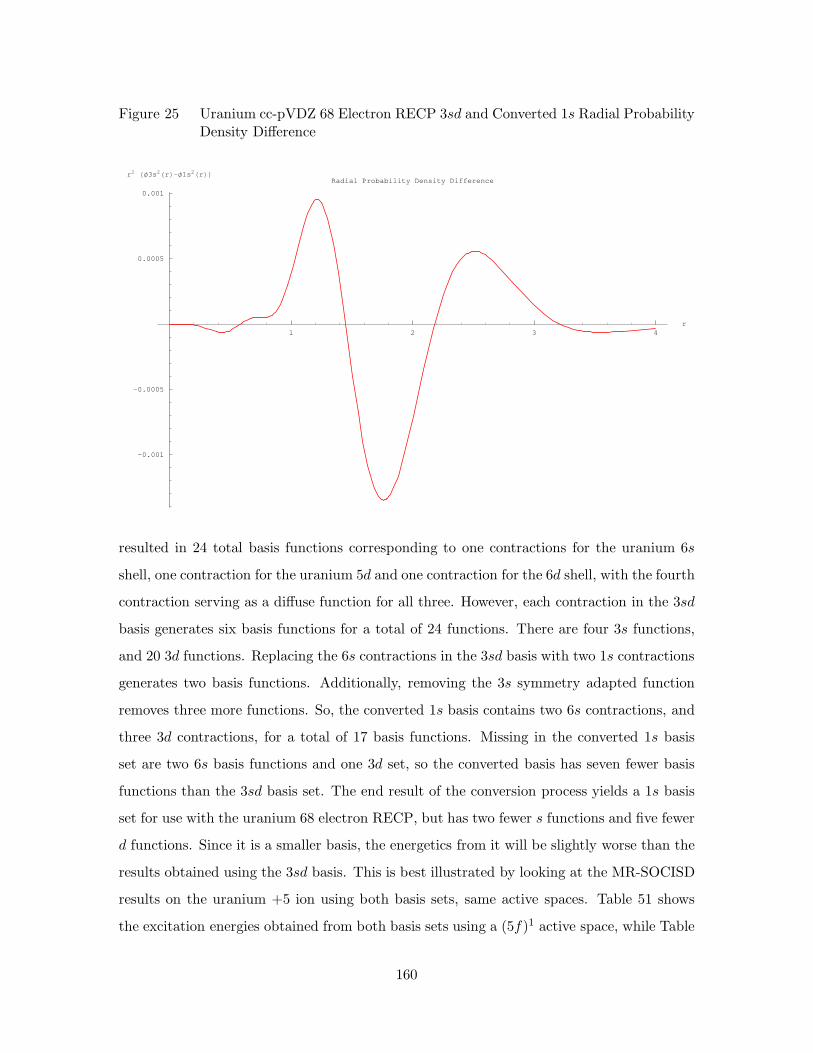
Figure 25 Uranium cc-pVDZ 68 Electron RECP 3sd and Converted 1s Radial ProbabilityDensity Difference
1 2 3 4r
-0.001
-0.0005
0.0005
0.001
r2 HΦ3s2HrL-Φ1s2HrLLRadial Probability Density Difference
resulted in 24 total basis functions corresponding to one contractions for the uranium 6s
shell, one contraction for the uranium 5d and one contraction for the 6d shell, with the fourth
contraction serving as a diffuse function for all three. However, each contraction in the 3sd
basis generates six basis functions for a total of 24 functions. There are four 3s functions,
and 20 3d functions. Replacing the 6s contractions in the 3sd basis with two 1s contractions
generates two basis functions. Additionally, removing the 3s symmetry adapted function
removes three more functions. So, the converted 1s basis contains two 6s contractions, and
three 3d contractions, for a total of 17 basis functions. Missing in the converted 1s basis
set are two 6s basis functions and one 3d set, so the converted basis has seven fewer basis
functions than the 3sd basis set. The end result of the conversion process yields a 1s basis
set for use with the uranium 68 electron RECP, but has two fewer s functions and five fewer
d functions. Since it is a smaller basis, the energetics from it will be slightly worse than the
results obtained using the 3sd basis. This is best illustrated by looking at the MR-SOCISD
results on the uranium +5 ion using both basis sets, same active spaces. Table 51 shows
the excitation energies obtained from both basis sets using a (5f)1 active space, while Table
160
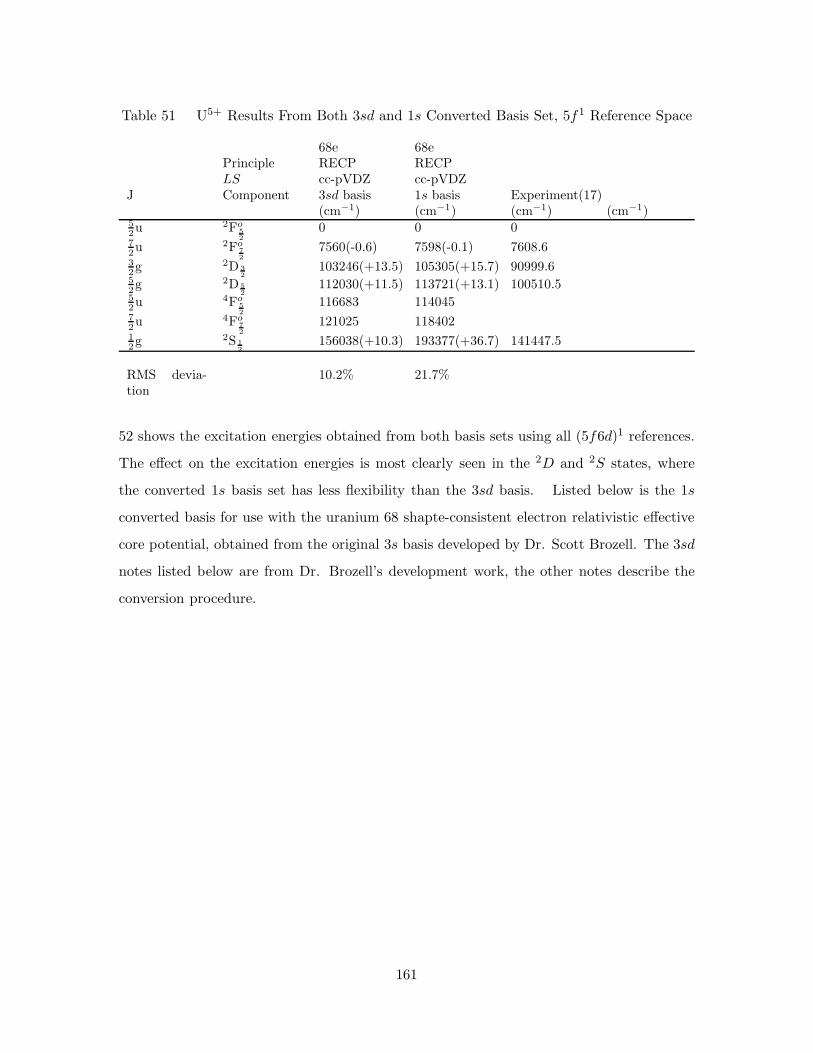
Table 51 U5+ Results From Both 3sd and 1s Converted Basis Set, 5f1 Reference Space
68e 68ePrinciple RECP RECPLS cc-pVDZ cc-pVDZ
J Component 3sd basis 1s basis Experiment(17)(cm−1) (cm−1) (cm−1) (cm−1)
5
2u 2Fo
5
2
0 0 07
2u 2Fo
7
2
7560(-0.6) 7598(-0.1) 7608.63
2g 2D 3
2
103246(+13.5) 105305(+15.7) 90999.65
2g 2D 5
2
112030(+11.5) 113721(+13.1) 100510.55
2u 4Fo
5
2
116683 1140457
2u 4Fo
7
2
121025 1184021
2g 2S 1
2
156038(+10.3) 193377(+36.7) 141447.5
RMS devia-tion
10.2% 21.7%
52 shows the excitation energies obtained from both basis sets using all (5f6d)1 references.
The effect on the excitation energies is most clearly seen in the 2D and 2S states, where
the converted 1s basis set has less flexibility than the 3sd basis. Listed below is the 1s
converted basis for use with the uranium 68 shapte-consistent electron relativistic effective
core potential, obtained from the original 3s basis developed by Dr. Scott Brozell. The 3sd
notes listed below are from Dr. Brozell’s development work, the other notes describe the
conversion procedure.
161

Table 52 U5+ Results From Both 3sd and 1s Converted Basis Set, (5f6d)1 ReferenceSpace
68e 68ePrinciple RECP RECPLS cc-pVDZ cc-pVDZ
J Component 3sd basis 1s basis Experiment(17)(cm−1) (cm−1) (cm−1) (cm−1)
5
2u 2Fo
5
2
0 0 07
2u 2Fo
7
2
7578(-0.4) 7615(+0.1) 7608.63
2g 2D 3
2
92570(+1.7) 95671(+5.1) 90999.65
2g 2D 5
2
101403(+0.9) 104179(+3.7) 100510.55
2u 4Fo
5
2
116809 1141627
2u 4Fo
7
2
121471 1185191
2g 2S 1
2
146989(+3.9) 191357(+35.3) 141447.5
RMS devia-tion
2.2% 17.9%
162
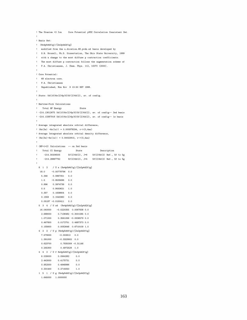
! The Uranium +2 Ion Core Potential pVDZ Correlation Consistent Set
!
! Basis Set:
! (8s4p5d4f1g)/[2s2p4d2f1g]
! modified from the u.dication.68.pvdz.sd basis developed by
! S.R. Brozell, Ph.D. Dissertation, The Ohio State University, 1999
! with a change to the most diffuse p contraction coefficients.
! The most diffuse p contraction follows the augmentation scheme of
! P.A. Christiansen, J. Chem. Phys. 112, 10070 (2000).
!
! Core Potential:
! 68 electron core.
! P.A. Christiansen
! Unpublished, Mon Nov 9 13:50 EST 1998.
!
! State: 5d(10)6s(2)6p(6)5f(2)6d(2), av. of config.
!
! Hartree-Fock Calculations
! Total HF Energy State
! -214.13612675 5d(10)6s(2)6p(6)5f(2)6d(2), av. of config-- 3sd basis
! -214.13387918 5d(10)6s(2)6p(6)5f(2)6d(2), av. of config-- 1s basis
!
! Average integrated absolute orbital difference,
! |6s(3s) -6s(1s)| = 0.000978334, r->(0,4au)
! Average Integrated aboslute orbital density difference,
! |6s(3s)-6s(1s)| = 0.00022913, r->(0,4au)
!
! (HF+1+2) Calculations -- on 3sd basis
! Total CI Energy State Description
! -214.30206505 5f(2)6d(2), J=6 5f(2)6d(2) Ref., 5f to 5g
! -214.28867792 5f(2)6d(2), J=4 5f(2)6d(2) Ref., 5f to 5g
!
8 1 2 / U s (8s4p5d4f1g)/[2s2p4d2f1g]
18.0 -0.00778796 0.0
5.346 0.0867051 0.0
1.5 -0.9535696 0.0
0.896 0.3974739 0.0
0.5 0.9553621 1.0
0.357 0.1838804 0.0
0.1559 0.1543360 0.0
0.05187 -0.0150411 0.0
5 3 4 / U sd (8s4p5d4f1g)/[2s2p4d2f1g]
16.040000 -0.0220355 0.0067838 0.0
2.688000 0.7136482 -0.3001085 0.0
1.071000 0.3561056 -0.0536579 0.0
0.467800 0.0172751 0.4687373 0.0
0.155600 0.0052648 0.6719109 1.0
4 2 2 / U p (8s4p5d4f1g)/[2s2p4d2f1g]
7.579000 -0.002612 0.0
1.391000 -0.3323902 0.0
0.623700 0.7835309 -0.31146
0.245300 0.4972529 1.0
4 4 2 / U f 8s4p5d4f1g)/[2s2p4d2f1g]
6.539000 0.0944382 0.0
2.443000 0.4175731 0.0
0.952000 0.4948986 0.0
0.331400 0.2716050 1.0
1 5 1 / U g (8s4p5d4f1g)/[2s2p4d2f1g]
1.645000 1.0000000
163
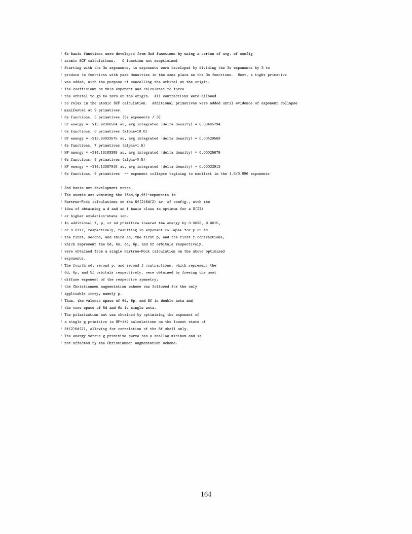
! 6s basis functions were developed from 3sd functions by using a series of avg. of config
! atomic SCF calculations. G function not reoptimized
! Starting with the 3s exponents, 1s exponents were developed by dividing the 3s exponents by 3 to
! produce 1s functions with peak densities in the same place as the 3s functions. Next, a tight primative
! was added, with the purpose of cancelling the orbital at the origin.
! The coefficient on this exponent was calculated to force
! the orbital to go to zero at the origin. All contractions were allowed
! to relax in the atomic SCF calculation. Additional primatives were added until evidence of exponent collapse
! manifested at 9 primatives.
! 6s functions, 5 primatives (3s exponents / 3)
! HF energy = -213.92366504 au, avg integrated |delta density| = 0.00465794
! 6s functions, 6 primatives (alpha=18.0)
! HF energy = -213.93923575 au, avg integrated |delta density| = 0.00429569
! 6s functions, 7 primatives (alpha=1.5)
! HF energy = -214.13183388 au, avg integrated |delta density| = 0.00025679
! 6s functions, 8 primatives (alpha=0.5)
! HF energy = -214.13387918 au, avg integrated |delta density| = 0.00022913
! 6s functions, 9 primatives -- exponent collapse begining to manifest in the 1.5/0.896 exponents
! 3sd basis set development notes
! The atomic set wamizing the (5sd,4p,4f)-exponents in
! Hartree-Fock calculations on the 5f(2)6d(2) av. of config., with the
! idea of obtaining a d and an f basis close to optimum for a U(II)
! or higher oxidation-state ion.
! An additional f, p, or sd primitive lowered the energy by 0.0023, 0.0015,
! or 0.0117, respectively, resulting in exponent-collapse for p or sd.
! The first, second, and third sd, the first p, and the first f contractions,
! which represent the 5d, 6s, 6d, 6p, and 5f orbitals respectively,
! were obtained from a single Hartree-Fock calculation on the above optimized
! exponents.
! The fourth sd, second p, and second f contractions, which represent the
! 6d, 6p, and 5f orbitals respectively, were obtained by freeing the most
! diffuse exponent of the respective symmetry;
! the Christiansen augmentation scheme was followed for the only
! applicable irrep, namely p.
! Thus, the valence space of 6d, 6p, and 5f is double zeta and
! the core space of 5d and 6s is single zeta.
! The polarization set was obtained by optimizing the exponent of
! a single g primitive in HF+1+2 calculations on the lowest state of
! 5f(2)6d(2), allowing for correlation of the 5f shell only.
! The energy versus g primitive curve has a shallow minimum and is
! not affected by the Christiansen augmentation scheme.
164
Vita
Major Eric V. Beck graduated from Carson City High School in Carson City, Nevada
in 1989. He completed a Bachelor of Science degree with a dual major in physics and mathe-
matics at the University of Nevada, Reno in May 1993. He received is M.S. degree in Nuclear
Engineering in March of 2003 from AFIT. Major Beck joined the United States Air Force
in May of 1995, and was commissioned in August 1995 at Officer Training School, Maxwell
Air Force Base (AFB), Alabama. His first assignment was at the Air Force Research Lab-
oratory, Space Vehicles Directorate in the Astrodynamics branch, Kirtland AFB, lasting
from October 1995 through April 1998. While stationed at Kirtland AFB, Major Beck co-
authored the Orbit Analysis Software Survey. He also assisted data acquisition and analysis
for high-accuracy orbit determination using angles-only data obtained from the low-cost
RAVEN telescope. In addition, he functioned as the laboratory’s representative to NASA
Lewis Research Center’s Breakthrough Propulsion Physics Steering Group. Following his
assignment at Kirtland AFB, Maj Beck was assigned to the Air Force Information Warfare
Center (AFIWC) at Lackland AFB, Texas. While stationed at AFIWC, Maj Beck served as
a project engineer in Radio Frequency Measurements branch of the Systems and Analysis
directorate. Here, he worked on test and measurement of local San Antonio radio and tele-
vision signals, the MC-130H AN/APQ-170 multimode radar, and the C-130J AN/APN-241
multimode radar. Following this duty, Maj Beck moved to the Radar and Communications
Analysis Flight of the 453rd Electronic Warfare Squadron, where he contributed to the Air
War Over Serbia (AWOS) Radar Warning Receiver (RWR) effectiveness after-action report
and C-17 collision avoidance system upgrade vulnerability analysis. He is currently serving
as a Stockpile Associate for the Defense Threat Reduction Agency at Lawerence Livermore
National Laboratory.
Permanent address: Lawrence Livermore National Laboratory7000 East Ave, L-159Livermore, CA 94551-9234
165

Bibliography
1. NIST Computational Chemistry Comparison and Benchmark Database. Technical Re-port, August 2005. NIST Standard Reference Database Number 101.
2. Adamo, Carlo and Vincenzo Barone. “Toward reliable density functional methodswithout adjustable parameters: The PBE0 model,” Journal of Chemical Physics,110 (13) (1999).
3. Addleman, R. Shane, et al. “On-Line Speciation of Uranyl Chelates in SupercriticalCO2 by Time-Resolved Laser-Induced Fluorescence Spectroscopy,” Analytical Chem-istry , 73 :1112–1119 (2001).
4. Altmann, Simon L. Rotations, Quaternions and Double Groups. Mineola, New York:Dover Publications, Inc., 2005.
5. Azenha, M. E., et al. “The Influence of an Effective Charge on the Uranate Lu-minescence in the Ordered Perovskite Structure,” Journal of Solid State Chemistry ,101 :190–194 (1992).
6. Balasubramanian, K. Handbook on the Physics and Chemistry of Rare Earths, 18 ,29. 1994.
7. Balasubramanian, K. Relativistic Effects in Chemistry, Part A: Theory and Tech-niques. John Wiley and Sons, Inc., 1997.
8. Barandiaran, Zolia and Luis Seijo. “Quantum chemical analysis of the bond lengths infn and fn−1d1 states of Ce3+, Pr3+, Pa4+ and U4+ defects in chloride hosts,” Journalof Chemical Physics, 119 (7):3785–3790 (2003).
9. Beck, Eric V. Theoretical Comparison of the excited electronic states of the uranyl(UO2+
2 ) and uranate (UO2−4 ) ions using relativistic computational methods. MS thesis,
Air Force Institute of Technology, 2003.
10. Becke, A. D. “A multicenter numerical integration scheme for polyatomic molecules,”Journal of Chemical Physics, 88 (4):2547–2553 (1987).
11. Becke, A.D. Physical Review A, 88 (1988).
12. Becke, A.D. “Density-functional thermochemistry. III. The role of exact exchange,”Journal of Chemical Physics, 98 (7) (1993).
13. Berg, Jacqueline O., et al. “Identification of U III and U IV Lines,” Journal of theOptical Society of America, 70 (6):716–719 (1980).
14. Bethe, H. A. and E. E. Salpeter. Quantum Mechanics of One- and Two-ElectronAtoms. Springer-Verlag, 1957.
15. Biemont, E., et al. “Relativistic Hartree-Fock and Dirac-Fock atomic structure calcu-lations in Fr-like ions Ra+, Ac2+, Th3+, and U5+,” Journal of Physics B: Atomic andMolecular Optical Physics, 37 :4193–4204 (2004).
16. Bjorken, J. D. and S. D. Drell. Relativistic Quantum Mechanics. McGraw-Hill BookCompany, 1964.
166
17. Blaise, Jean and Jean-Francois Wyart, “Selected Constants Energy Levels and AtomicSpectra of Actinides,” 2004. http://www.lac.u-psud.fr/Database/Contents.html.
18. Blasse, G. “The Structure Sensitivity of the U6+ Ion Luminescence in Oxides,” Journalof the Electrochemical Society , 124 (8):1280–1284 (1977).
19. Blasse, G., et al. “The Luminescence of Hexavalent Uranium in Solids,” Journal ofLuminescence, 18/19 :57–62 (1979).
20. Blaudeau, J.-P., et al. “Atomic Orbital Basis Sets for Use with Effective Core Poten-tials,” International Journal of Quantum Chemistry, 77 :516–520 (2000).
21. Blaudeau, J-P and L.A. Curtiss. “Optimized Gaussian Basis Sets for Use with Rel-ativistic Effective (Core) Potentials,” Internation Journal of Quantum Chemistry,61 :943–952 (1997).
22. Bleijenberg, K. C. “Charge transfer transitions within the octahedral uranate group,”Journal of Chemical Physics, 73 (2):617–621 (1980).
23. Brewer, Leo. “Eneriges of the Electronic Configurations of the Singly, Doubly, andTriply Ionized Lanthanides and Actinides,” Journal of the Optical Society of America,61 (12):1666–1682 (1971).
24. Brooks, B. R., et al. “The Loop-Driven Graphical Unitary Group Approach: A Power-ful Method for the Variational Description of Electron Correlation,” Physica Scripta,21 :312–322 (1980).
25. Brozell, Scott R. Spin-Orbit Configuration Interaction Calculations of Actinide andLanthanide Systems. PhD dissertation, Ohio State University, 1999.
26. Burns, Peter C., et al. “The Crystal Chemistry of Hexavalent Uranium: PolyhedronGeometries, Bond-Valence Parameters, and Polymerization of Polyhedra,” The Cana-dian Mineralogist , 35 :1551–1570 (1997).
27. Burns, Peter C., et al. “U6+ Minerals and Inorganic Phases: A Comparison andHierarchy of Crystal Structures,” The Canadian Mineralogist , 34 :845–880 (1996).
28. Cao, X. and M. Dolg. “Theoretical prediction of the second to fourth actinide ionizationpotentials,” Molecular Physics, 101 (7):961–969 (2003).
29. Carnall, William T., et al. Gmelin Handbook of Inorganic Chemistry (8th Edition),A5 . Springer-Verlag, 1982.
30. Ceperley, D. M. and B. J. Alder. “Ground State of the Electron Gas by a StochasticMethod,” Physical Review Letters, 45 (7):566–569 (1980).
31. Chrisiansen, P. A. “Basis sets in correlated effective potential calculations,” Journalof Chemical Physics, 112 (23):10070–10074 (2000).
32. Clark, Aurora E., et al. “Density and wave function analysis of actinide complexes:What can fuzzy atom, atoms-in-molecules, Mulliken, Lowdin, and natural populationanalysis tell us?,” Journal of Chemical Physics, 121 (6):2563–2570 (2004).
33. Clavaguera, Carine, et al. “Modeling Complexes of the Uranyl Ion UO2Ln+2 : Bind-
ing Energies, Geometries, and Bonding Analysis,” Journal of Chemical Physics A,107 :4515–4525 (2003).
167

34. Clavaguera, Carine, et al. “Calculation of harmonic and anharmonic vibrationalwavenumbers for triatomic uranium compounds XUY,” Chemical Physics, 302 :1–11(2004).
35. Cohen-Tannoudji, C., et al. Quantum Mechanics, Volume I . Hermann and John Wileyand Sons, Inc., 1977.
36. Conway, John G. and Earl F. Worden. “Isotope shift of uranium in the infrared regionbetween 1817 and 5598 cm−1,” Journal of the Optical Society of America, 1 (6):788–794(1984).
37. Cook, David B. Handbook of Quantum Chemistry . Dover Publications Inc., 2005.
38. Cordfunke, E. H. P. and D. J. W. IJdo. “α- and β-Na2UO4: Structural and Thermo-chemical Relationships,” Journal of Solid State Chemistry , 115 :299–304 (1995).
39. de Jong, W. A., et al. “Fully relativistic correlated benchmark results for uranyl and acritical look at relativistic effective core potentials for uranium,” Theoretical ChemicalAccounts, 107 :22–26 (2001).
40. den Berge, Sven Van, et al. “The Local Uranium Environment in Cesium Uranates:A Combined XPS, XAS, XRD, and Neutron Diffraction Analysis,” Journal of SolidState Chemistry , 166 :320–329 (2002).
41. Denning, R. G. Electronic Structure and Bonding in Actinyl Ions, 79 , 217–273. Berlin:Springer-Verlag, 1992.
42. Denning, R. G., et al. “The electronic structure of the uranyl ion Part I. The electronicspectrum of Cs2UO2Cl4,” Molecular Physics, 32 (2):419–442 (1976).
43. Denning, R. G., et al. “The electronic structure of the uranyl ion II. The electronicspectra of CsUO2(NO3)3 and NaUO2(CH3COO)3,” Molecular Physics, 37 (4):1089–1107 (1979).
44. Denning, R. G., et al. “Covalency in the uranyl ion: A polarized x-ray spectroscpicstudy,” Journal of Chemical Physics, 117 (17) (2002).
45. Denning, R. G., et al. “The electronic structure of the uranyl ion III. Theory,” Molec-ular Physics, 37 (4):1109–1143 (1979).
46. Deurzen, C. H. H. Van, et al. “Uranium five (U V), the 1S0 level, and a paramet-ric analysis of the 5f2 configuration,” Journal of the Optical Society of America B ,1 (1):45–47 (1984).
47. Dirac, P. A. M. “The Quantum Theory of the Electron,” Proceedings of the RoyalSociety London, Series A, 118 :610–624 (1928).
48. Dirac, P. A. M. “The Quantum Theory of the Electron, Part II.,” Proceedings of theRoyal Society London, Series A, 118 :351–361 (1928).
49. Docrat, T. I., et al. “X-ray Absorption Spectroscopy of Tricarbonatodioxouranate(V),[UO2(CO3)3]
5−, in Aqueous Solution,” Inorganic Chemistry , 38 :1879–1882 (1999).
50. Dolg, Michael. Effective core potentials, 79 , 479–508. Julich: John von NeumannInstitute for Computing, 2000.
168
51. Dolg, Michael and Xiaoyan Ciao. The Relativistic Energy-Consistent ab initio Pseu-dopotential Approach and Its Application to Lnathanide and Actinide Compounds,1–36. World Scientific, 2004.
52. Duch, W. “The Direct Configuration Interaction Method for General Multirefer-ence Expansions: Symmetric Group Approach,” Theoretica Chimica Acta, 57 :299–313(1980).
53. Eliav, Ephraim and Uzi Kaldor. “Relativistic coupled-cluster method: Intrashell exci-tations in the f2 shells of Pr3+ and U4+,” Physical Review A, 51 (1):225–229 (1995).
54. Ermler, W. C., et al. “Ab Initio Relativistic Effective Potentials with Spin-OrbitOperators. VI. Fr through Pu,” International Journal of Quantum Chemistry, 40 :829–846 (1991).
55. Fedorov, Dmitri G., et al. “An ab initio study of excited states of U and UF,” Journalof Chemical Physics, 118 (11):4970–4975 (2003).
56. Fefee, L. A., et al., “Clarkson Univeristy Relativistic Effective Potential Database.”
57. Gagliardi, Laura and Bjorn O. Roos. “Uranium triatomic compounds XUY (X, Y= C, N, O): a combined multiconfigurational second-order perturbation and densityfunctional study,” Chemical Physics Letters, 331 :229–234 (2000).
58. Gerloch, M. Orbitals, Terms and States. John Wiley and Sons, 1986.
59. Gill, Peter M. W., et al. “A standard grid for density functional calculations,” ChemicalPhysics Letters, 209 (5,6):506–512 (1993).
60. Green, Jennifer C., et al. “Electronic Structure of M(BH4)4, M= Zr, Hf, and U, byVariable Photon-Energy Photoelectron Spectroscopy and Density Functional Calcula-tions,” Inorganic Chemistry , 44 :7781–7793 (2005).
61. Griffiths, Trevor R. and Vladimir A. Volkovich. “A review of the high temperatureoxidation of uranium oxides in molten salts and in the solid state to forum alkalimetal uranates, and their composition and properties,” Journal of Nuclear Materials,274 :229–251 (1999).
62. Grimme, Stefan. “Density functional calculations with configuration interaction forthe excited states of molecules,” Chemical Physics Letters, 259 :128–137 (1996).
63. Grimme, Stefan and Mirko Waletzke. “A combination of Kohn–Sham density func-tional theory and multi-reference configuration interaction methods,” The Journal ofChemical Physics, 111 (13):5645–5655 (1999).
64. Han, Young-Kyu and Kimihiko Hirao. “Density functional studies of UO2+2 and AnF6
(An=U, Np, and Pu) using scalar-relativistic effective core potentials,” Journal ofChemical Physics, 113 (17) (2000).
65. Handy, N. C. and S. F. Boys. “Integration Points for the Reduction of BoundaryConditions,” Theoretical Chimica Acta, 31 :195–200 (1973).
66. Harrison, R. J. Computational chemistry for nuclear waste characterization and pro-cessing: Relativistic quantum chemisty of actinides. Technical Report, U.S. Depart-ment of Energy, 1999.
169
67. Herzberg, G. Molecular Spectra and Molecular Structure I. Spectra of DiatomicMolecules. Van Nostrand Reinhold Company, 1950.
68. Hess, Bernd A. Valence-Only Effective Hamiltonians, 79 , 106–117. John Wiley andAssociates, 2003.
69. Hoekstra, H. and S. Siegel. “Structural Studies on Li4UO5 and Na4UO5,” Journal ofInorganic Nuclear Chemistry , 26 :693–700 (1964).
70. Hohenberg, P. and W. Kohn. “Inhomogeneous Electron Gas,” Physical Review ,136 (3B):864–871 (1964).
71. Huber, K.P. and G. Herzberg. NIST Chemistry WebBook , chapter Constants of Di-atomic Molecules. June 2005. NIST Standard Reference Database Number 69.
72. Ismail, Nina, et al. “Theoretical Studies of the actinides: method calibration for theUO2+
2 and PuO2+2 ions,” Chemical Physics Letters, 300 :296–302 (1999).
73. Kaltsoyannis, N. “Relativistic Effects in organic and organometallic chemistry,” Jour-nal of the Chemical Society, Dalton Transactions, 1–11 (1997).
74. Kaltsoyannis, Nikolas. “Computational Study of Analogues of the Uranyl IonContaining the -N=U=N- Unit: Density Functional Theory Calculations onUO2+
2 , UON+, UN2, UO(NPH3)3+, U(NPH3)
4+2 , [UCl4NPR32] (R=H, Me), and
[UOCl4NP(C6H5)3]−,” Inorganic Chemistry , 39 :6009–6017 (2000).
75. Katz, J. J., et al. The Chemistry of the Actinide Elements (2nd Edition). Chapmanand Hall Ltd., 196.
76. Kleinschmidt, Martin, et al. “Spin-Orbit Coupling of DFT/MRCI Wavefunctions:Method, Test Calculations, and Application to Thiophene,” Journal of ComputationalChemistry , 83 :824–833 (2002).
77. Kleinschmidt, Martin, et al. “SPOCK.CI: A Multireference Spin Orbit Config-uration Interaction Method for Large Molecules,” Journal of Chemical Physics,124 (2006):124101 (2006).
78. Koch, et al. A Chemist’s Guide to Density Functional Theory (2nd Edition). Wein-heim, Federal Republic of Germany: Wiley-VCH, 2001.
79. Kohn, W. and L. J. Sham. “Self-Consistent Equations Including Exchange and Cor-relation Effects,” Physical Review A, 140 (4A):1133–1138 (1965).
80. Krol, D. M. and G. Blasse. “Luminescence and energy migration in Ba2CaUO6,”Journal of Chemical Physics, 69 (7):3124–3127 (1978).
81. Lee, C., et al. “Development of Colle-Salvetti Correlation-energy Formula Into a Func-tional of the Electron Density,” Physical Review B , 37 (2) (1988).
82. Lischka, Hans, et al. “High-level multireference methods in the quantum-chemistryprogram system COLUMBUS: Analytic MR-CISD and MR-AQCC gradients and MR-AQCC-LRT for excited states, GUGA spin-orbit CI and parallel CI density,” PhysicalChemistry Chemical Physics, 3 :664–673 (2000).
170
83. Lue, Christopher J., et al. “Electronic Spectroscopy of UO2 Isolated in a Solid ArMatrix,” Journal of the American Chemical Society , 126 :1812–1815 (2004).
84. Mahurin, S. M., et al. “Spectroscopic determination of heterogeneities in uranyl-dopedglasses,” Journal of Non-Crystalline Solids, 325 :70–75 (2003).
85. Matsika, S., et al. “Electronic Structure and Spectra of Actinyl Ions,” Journal ofPhysical Chemistry A, 105 :3825–3828 (2001).
86. Matsika, Spiridoula and Russell M. Pitzer. “Actinyl Ions in Cs2UO2Cl4,” J. PhysicalChemistry A, 105 :637–645 (2001).
87. Mattsson, A. E. Science, 298 (2002).
88. Messiah, A. Quantum Mechanics. Dover Publications, 1999.
89. Miller, Mark L., et al. “Description and classification of uranium oxide hydrate sheetanion topologies,” Journal of Materials Research, 11 (12):3048–3056 (1996).
90. Miyabe, Masabumi, et al. “Total angular momenta of even-parity autoionizing levelsand odd-parity high-lying levels of atomic uranium,” Journal of Physics B: Atomic,Molecular and Optical Physics, 35 (2002).
91. Miyabe, Masabumi, et al. “Highly excited odd-parity levels of atomic uranium,” Jour-nal of Physics B: Atomic, Molecular and Optical Physics, 33 :4957–4972 (2000).
92. Miyoshi, E., et al. Recent Developments of Relativistic Model Core Potentials, 37–64.World Scientific, 2004.
93. Morozov, A. M. and D. F. Smolina. “Incorporation of Uranium into Single Crystalsof Tungstates with the Scheelite Structure,” Neoganicheskie Materialy , 14 (1):125–127(1978).
94. Morozova, L. G. and P. P. Feofilov. “Temperature quenching of uranium luminescencein scheelite-type single crystals,” Optics and Spectroscopy , 35 (4):458–459 (1973).
95. M.S.Gordon and M.W.Schmidt. Advances in electronic structure theory: GAMESS adecade later . Amsterdam: Elsevier, 2005.
96. Mura, Michael E. and Peter J. Knowles. “Improved radial grids for quadra-ture in molecular density-functional calculations,” Journal of Chemical Physics,104 (24):9848–9858 (1996).
97. Murray, Christopher W., et al. “Quadrature schemes for integrals of density functionaltheory,” Molecular Physics, 78 (4):997–1014 (1993).
98. M.W.Schmidt, et al. “General Atomic and Molecular Electronic Structure System,”Journal of Computational Chemistry, 14 :1347–1363 (1993).
99. Onopko, D. E., et al. “Origin of red luminescence in scheelite crystals activated withuranium,” Optics and Spectroscopy , 38 (6):658–659 (1975).
100. Palmer, Byron A. and Jr. Rolf Engleman. “Wavelengths and energy levels of doublyionized uranium (U III) obtained using a Fourier-transform spectrometer,” Journal ofthe Optical Society of America B , 1 (4):609–625 (1984).
171

101. Pepper, M and B E Bursten. “The electronic structure of actinide-containing molecules:A challenge to applied quantum chemistry,” Chem. Rev., 91 :719–741 (1991).
102. Perdew, John P. and Matthias Ernzerhof. “Rational for mixing exact exchange withdensity functional approximations,” Journal of Chemical Physics, 105 (22) (1996).
103. Perdew, John P. and Karla Schmidt. Density Functional Theory and Its Applicationsto Materials. American Institute of Physics, 2001.
104. Petersson, George A., et al. “On the Optimization of Gaussian Basis Sets,” Journalof Chemical Physics, 118 (3):1101–1109 (2003).
105. Pierloot, Kristine. “The CASPT2 method in inorganic electronic spectroscopy:from ionic transition metal to covalent actinde complexes,” Molecular Physics,101 (13):2083–2094 (2003).
106. Pilar, Frank L. Elementary Quantum Chemistry (2nd Edition). Dover PublicationsInc., 1990.
107. Pitzer, Kenneth S. “Relativistic Effects on Chemical properties,” Accounts of ChemicalResearch, 12 (8) (1979).
108. Pyykko, P. “Relativistic Effects in Structural Chemistry,” Chemical Reviews, 88 :563–594 (1988).
109. Pyykko, P. and J.-P. Desclaux. “Relativity and the periodic system of elements,” Acc.Chem. Res., 12 :276–281 (1979).
110. R. Shepard, I. Shavitt, R. M. Pitzer, D. C. Comeau, M. Pepper, H. Lischka, P. G.Szalay, R. Ahlrichs, F. B. Brown, and J.-G. Zhao. “A Progress Report on the Statusof the COLUMBUS MRCI Program System,” Int. J. Quantum Chem., 22 :149–165(1988).
111. Rabinowitch, Eugene and R. Linn Belford. Spectroscopy and Photochemistry of UranylCompounds. Pergamon Press Inc., 1964.
112. Raghavachari, K. and J. B. Anderson. “Electron Correlation Effects in Molecules,”Journal of Physical Chemistry, 100 :12960–12973 (1996).
113. Roos, B. “A New Method for Large-Scale CI Calculations,” Chemical Physics Letters,15 (2):153–159 (1972).
114. Roothaan, C. C. J. “New Developments in Molecular Orbital Theory,” Reviews inModern Physics, 23 :69–89 (1951).
115. Roothaan, C. C. J. “Self-Consistent Field Theory for Open Shells of Electronic Sys-tems,” Reviews in Modern Physics, 32 :179–185 (1960).
116. Sawyer, J. O. “The crystal structure of α SrUO4.000,” Journal of Inorganic NuclearChemistry , 34 :3268–3271 (1972).
117. Schnedier, Richard T. and Timothy E. Roxey. “Wavelengths of U III and U IV linesin the near ultraviolet,” Applied Optics, 21 (23):4204–4206 (1982).
172
118. Seijo, Luis and Zoila Barandiaran. “Ab initio theoretical studies on U3+ and on thestructure and spectroscopy of U3+ substitutional defects in Cs2NaYCl6,” Journal ofChemical Physics, 118 (2003).
119. Shavitt, I. Annual Report on New Methods in Computational Quantum Chemistryand Their Application on Modern Super-computers. Technical Report, NASA AmesResearch Center, 1979.
120. Shavitt, I. The Graphical Unitary Group Approach and It’s Application to DirectConfiguration Interaction Calculations, 51–99. Springer-Verlag, 1981.
121. Shavitt, I. The Unitary Group and the Electron Correlation Problem, 279–293. 1983.
122. Shavitt, I. “The Graphical Representation in GUGA.” Unpublished lecture notes,2005.
123. Shavitt, I. “Introduction to the Unitary Group Approach.” Unpublished lecture notes,2005.
124. Shavitt, I. “Matrix-Element Calculus in GUGA.” Unpublished lecture notes, 2005.
125. Stoll, Hermann. “Large-core vs. small-core pseudopotentials: A case study for Au2,”Chemical Physics Letters, 429 :289–293 (2006).
126. Stoll, Hermann, et al. “Relativistic Energy-Consistent PseudopotentialsRecent Devel-opments,” Journal of Computational Chemistry, 23 :767–778 (2002).
127. Szabo, Attila and Neil S. Ostlund. Modern Quantum Chemistry Introduction to Ad-vanced Structure Theory . Mineola, New York: Dover Publications, Inc., 1989.
128. Takahashi, Kazuo, et al. “Crystal Chemical and Thermodynamic Study on CaUO4−x,(Ca0.5Sr0.5UO4−x, and α-SrUO4−x (x = 0 - 0.5),” Journal of Solid State Chemistry ,105 :234–246 (1993).
129. Tanner, Peter A., et al. “Luminescence of the uranyl-ion-doped elpasolite lattice,”Journal of Physics: Condensed Matter , 13 :189–194 (2001).
130. Tanner, Peter A., et al. “Luminescence of the uranyl-ion-doped strontium tetraborate(SrB4O7),” Journal of the Physical Chemistry of Solids, 58 (7):1143–1146 (1997).
131. Tao, J. and J. P. Perdew. “Climbing the Density Functional Ladder: NonempiricalMeta-Generalized Gradient Approximation Designed for Molecules and Solids,” Phys-ical Review Letters, 91 (14):1464011–1464014 (2003).
132. Teterin, Yu A., et al. “Inner valence molecular orbitals and structure of the X-rayO4,5(Th,U) emission spectra in thorium and uranium oxides,” Journal of ElectronSpectroscopy and Related Phenomena, 96 :229–236 (1998).
133. Teterin, Yury A., et al. “The structure of the valence electronic orbitals in uraniumtrioxide γ-UO3,” Journal of Nuclear Science and Technology , 3 :74–77 (2002).
134. Veal, B. W., et al. “X-ray photoemission spectroscopy study of hexavalent uraniumcompounds,” Physical Review B , 12 (12):5651–5663 (1975).
135. Wang, Jiahu, et al. “Evaluation of⟨
S2⟩
in Restricted, Unrestricted Hartree-Fock andDensity Functional Based Theories,” Journal of Chemical Physics, 102 (8) (1995).
173
136. Wang, Zheming, et al. “Cryogenic Laser Induced Fluorescence Characterization ofU(VI) In Hanford Vadose Zone Pore Waters,” Environmental Science and Technology ,38 :5591–5597 (2004).
137. Wanner, H. and I. Forest, editors. Chemical Thermodynamics of Uranium, 1 . ChemicalThermodynamics. North-Holland Elsevier Science Publishers, 1992.
138. Wilson, S. The Dirac Equation and Dirac Spectrum, 1 , 200–209. 2003.
139. Wyart, J. F., et al. “Analysis of the Spectrum of Four-Times-Ionized Uranium (U5),”Physica Scripta, 22 :389–396 (1980).
140. Yutsis, A. P., et al. Mathematical Apparatus of the Theory of Angular Momentum, 1 ,390–429. 2003.
141. Zachariasen, W. H. “Crystal Chemical Studies of the 5f -Series of Elements. XXI. TheCrystal Structure of Magnesium Orthouranate,” Acta Crystallographica, 7 :788–791(1954).
142. Zhang, Z. and R. M. Pitzer Journal of Physical Chemistry A, 103 :6880–6886 (1999).
174

REPORT DOCUMENTATION PAGE Form Approved OMB No. 074-0188
The public reporting burden for this collection of information is estimated to average 1 hour per response, including the time for reviewing instructions, searching existing data sources, gathering and maintaining the data needed, and completing and reviewing the collection of information. Send comments regarding this burden estimate or any other aspect of the collection of information, including suggestions for reducing this burden to Department of Defense, Washington Headquarters Services, Directorate for Information Operations and Reports (0704-0188), 1215 Jefferson Davis Highway, Suite 1204, Arlington, VA 22202-4302. Respondents should be aware that notwithstanding any other provision of law, no person shall be subject to an penalty for failing to comply with a collection of information if it does not display a currently valid OMB control number. PLEASE DO NOT RETURN YOUR FORM TO THE ABOVE ADDRESS. 1. REPORT DATE (DD-MM-YYYY) 22-03-2007
2. REPORT TYPE Doctoral Dissertation
3. DATES COVERED (From – To) Apr 2003 – Mar 2007
5a. CONTRACT NUMBER
5b. GRANT NUMBER
4. TITLE AND SUBTITLE A Multireference Density Functional Approach To The Calculation Of The Excited States Of Uranium Ions
5c. PROGRAM ELEMENT NUMBER
5d. PROJECT NUMBER If funded, enter ENR # 5e. TASK NUMBER
6. AUTHOR(S) Beck, Eric V., Major, USAF 5f. WORK UNIT NUMBER
7. PERFORMING ORGANIZATION NAMES(S) AND ADDRESS(S) Air Force Institute of Technology Graduate School of Engineering and Management (AFIT/EN) 2950 Hobson Way WPAFB OH 45433-7765
8. PERFORMING ORGANIZATION REPORT NUMBER AFIT/DS/ENP/07-01
10. SPONSOR/MONITOR’S ACRONYM(S) DOE NEER
9. SPONSORING/MONITORING AGENCY NAME(S) AND ADDRESS(ES) Department of Energy, Idaho Operations Office Attn: Nancy Elizondo, Project Manager 1955 Fremont Ave MS 1235 Idaho Falls, ID 83401-1563
11. SPONSOR/MONITOR’S REPORT NUMBER(S)
12. DISTRIBUTION/AVAILABILITY STATEMENT APPROVED FOR PUBLIC RELEASE; DISTRIBUTION UNLIMITED.
13. SUPPLEMENTARY NOTES 14. ABSTRACT An accurate and efficient hybrid Density Functional Theory (DFT)/Multireference Configuration Interaction (MRCI) model for computing electronic excitation energies in heavy element atoms and molecules was developed. This model incorporated relativistic effects essential for accurate qualitative and quantitative spectroscopic predictions on heavy elements, while simultaneously removing spin-multiplicity limitations inherent in the original model on which it is based. This model was used to successfully compute ground and low-lying electronic states for atoms in the first two rows of the period table, which were used for calibration. Once calibrated, calculations on carbon monoxide, bromine fluoride, the bromine atom, uranium +4 and +5 ions and the uranyl (UO2
2+) ion showed the model achieved reductions in relative error with respect to Time Dependent Density Functional Theory (TDDFT) of 11-42%, with a corresponding reduction in computational effort in terms of MRCI expansion sizes of a factor of 25-64. 15. SUBJECT TERMS Relativistic quantum chemistry, uranium electronic spectroscopy, computational chemistry, density functional theory Multireference configuration interaction, time dependent density functional theory 16. SECURITY CLASSIFICATION OF:
19a. NAME OF RESPONSIBLE PERSON Dr. Larry W. Burggraf
REPORT U
ABSTRACT U
c. THIS PAGE U
17. LIMITATION OF ABSTRACT UU
18. NUMBER OF PAGES 190 19b. TELEPHONE NUMBER (Include area code)
(937) 255-3636 x 4507 e-mail: [email protected]
Standard Form 298 (Rev: 8-98) Prescribed by ANSI Std. Z39-18