Embed Size (px)
Citation preview

Celestial mechanics:
The perturbed Kepler problem.
Laszlo Arpad Gergely1,2
1 Department of Theoretical Physics, University of Szeged,
Tisza Lajos krt 84-86, Szeged 6720, Hungary2 Department of Experimental Physics, University of Szeged,
Dom Ter 9, Szeged 6720, Hungary
January 14, 2015
1

Completed with the support of the European Union and the State of Hun-gary, cofinanced by the European Social Fund in the framework of TAMOP4.2.4. A/2-11-/1-2012-0001 ‘National Excellence Program’
2

Contents
1 Introduction 5
2 Keplerian motion 6
2.1 The one-center problem . . . . . . . . . . . . . . . . . . . . . . . 62.2 Constants of motion . . . . . . . . . . . . . . . . . . . . . . . . . 72.3 The orbit . . . . . . . . . . . . . . . . . . . . . . . . . . . . . . . 8
2.3.1 Parametrization of the radial motion by the true anomaly 82.3.2 Conics . . . . . . . . . . . . . . . . . . . . . . . . . . . . . 92.3.3 Dynamical characterization of the periastron . . . . . . . 12
2.4 Solution of the equations of motion: the Kepler equation . . . . . 132.4.1 Circular and elliptic orbits . . . . . . . . . . . . . . . . . . 132.4.2 Parabolic orbits . . . . . . . . . . . . . . . . . . . . . . . . 142.4.3 Hyperbolic orbits . . . . . . . . . . . . . . . . . . . . . . . 142.4.4 The eccentric anomaly: a summary . . . . . . . . . . . . 15
2.5 Orbital elements . . . . . . . . . . . . . . . . . . . . . . . . . . . 162.6 Kinematical definition of the parametrizations for the elliptic and
parabolic motions . . . . . . . . . . . . . . . . . . . . . . . . . . . 172.6.1 Elliptic orbits . . . . . . . . . . . . . . . . . . . . . . . . . 192.6.2 Parabolic orbits . . . . . . . . . . . . . . . . . . . . . . . . 20
3 The perturbed two-body system 21
3.1 Lagrangian description of the perturbation . . . . . . . . . . . . . 213.2 Evolution of the Keplerian dynamical constants in terms of the
perturbing force . . . . . . . . . . . . . . . . . . . . . . . . . . . 213.3 Precession of the basis vectors in terms of the perturbing force . 233.4 Summary . . . . . . . . . . . . . . . . . . . . . . . . . . . . . . . 24
4 The Lagrange planetary equations 25
4.1 Evolution of the orbital elements in terms of the evolution ofKeplerian dynamical constants . . . . . . . . . . . . . . . . . . . 25
4.2 Evolution of the orbital elements in terms of the perturbing force 26
5 Orbital evolution under perturbations in terms of the true
anomaly 28
5.1 The perturbed Newtonian dynamical constants . . . . . . . . . . 285.2 The evolution of the Newtonian dynamical constants in terms of
the true anomaly . . . . . . . . . . . . . . . . . . . . . . . . . . . 305.3 Summary of the results obtained with the true anomaly parametriza-
tion . . . . . . . . . . . . . . . . . . . . . . . . . . . . . . . . . . 30
6 Orbital evolution under perturbations in terms of the eccentric
anomaly 32
6.1 The eccentric anomaly parametrization . . . . . . . . . . . . . . . 326.2 The evolution of the eccentric anomaly . . . . . . . . . . . . . . . 32
3
6.3 The evolution of the Newtonian dynamical constants for ξp-dependentperturbing forces . . . . . . . . . . . . . . . . . . . . . . . . . . . 336.3.1 A note on the circularity of the perturbed orbit . . . . . . 34
6.4 The Kepler equation in the presence of perturbations . . . . . . . 356.4.1 The radial period . . . . . . . . . . . . . . . . . . . . . . . 37
6.5 Summary . . . . . . . . . . . . . . . . . . . . . . . . . . . . . . . 37
7 Constant perturbing force 39
7.1 The evolution of the dynamical constants and of the radial period 397.1.1 Changes and averages over one radial period . . . . . . . 40
7.2 The Kepler equation . . . . . . . . . . . . . . . . . . . . . . . . . 417.3 The periastron shift . . . . . . . . . . . . . . . . . . . . . . . . . 42
7.3.1 Calculation based on the true anomaly . . . . . . . . . . . 427.3.2 Calculation based on the eccentric anomaly . . . . . . . . 437.3.3 Average precession rate . . . . . . . . . . . . . . . . . . . 45
7.4 Comment on the parametrizations . . . . . . . . . . . . . . . . . 457.5 Secular orbital evolution in the plane of motion . . . . . . . . . . 467.6 Secular evolution of the plane of motion . . . . . . . . . . . . . . 48
8 Equal mass binary perturbed by a small, center of mass located
body 50
A Computation details for subsection 5.1 50
4

1 Introduction
In Chapter 2 we review the basics of Keplerian motion in a form suitable forgeneralization to the perturbed case. The solution of the two-body problem isgiven both in terms of dynamical constants and orbital elements, however theaccent is put on the former, as this is what we want to explore in more detailin the perturbed case.
Chapter 3 contains the generic discussion of the perturbed two-body prob-lem. In some cases the perturbation can be related to a generalized Lagrangian(possibly depending on accelerations). We show how to derive the accelerationfrom such a Lagrangian. Then in the rest of the chapter we develop the equationsgoverning the slow evolution of the Newtonian constants and of the referencesystem constructed from them, in terms of the components of the perturbativeforce (irrespective of whether these arise or not from a Lagrangian). The evolv-ing Newtonian constants represent a sequence of Keplerian orbits with differentparameters, which match well the perturbed orbit at each point. The Keplerianorbit with varying parameters represents the osculating orbit, a notion usuallyemployed for the ellipse.
Chapter 4 relates the variation in time of the Keplerian dynamical constantsto the evolution of the orbital elements. The latter are known as the Lagrangeplanetary equations, equivalent with the evolution equations for the osculatingdynamical constants, provided a reference plane and a reference direction aresingled out.
In chapter 5 the osculating dynamical constants are derived explicitly interms of the true anomaly parametrization, which can be introduced exactlyas in the unperturbed case, due to a radial equation, which has an unmodifiedfunctional form as compared to the unperturbed equation. The functional formof the evolution law for the true anomaly however is modified.
In chapter 6 the eccentric anomaly is introduced exactly in the same way as inthe unperturbed case (same functional form). Its evolution is derived explicitlyand by a formal integration the dynamical law governing the perturbed motion,the perturbed Kepler equation, is established. In the process the osculatingdynamical constants are determined as function of the eccentric anomaly, theradial period of the perturbed motion is defined and the condition of circularityof perturbed Keplerian orbits is analyzed.
As a first application of the formalism derived, we consider a constant per-turbing force in chapter 7. Such a force can possibly act on a binary systemdue to a distant supermassive black hole. This computationally simple toymodel allows to explicitly perform all calculations presented only formally inthe previous chapters. The osculating dynamical constants are determined, theperiastron shift computed and the perturbed Kepler equation written up ex-plicitly. Another application is proposed as a problem to be developed by thestudents.
The gravitational constant G is kept in all expressions. A vector with anoverhat denotes a unit vector, the only exception under this rule being n = r/r.Time derivatives are denoted both by a dot or by d/dt.
5

2 Keplerian motion
The motion of two point masses under their mutual gravitational attraction ischaracterized by the one-center Lagrangian:
LN =µv2
2+Gmµ
r, (1)
where m = m1 + m2 is the total mass, µ = m1m2/m the reduced mass,r = r2 − r1 = rn, with r the relative distance and v the magnitude of therelative velocity v = pN/µ, pN= ∂LN/∂v being the relative momentum). TheLagrangian represents a particle of mass µ moving in the gravitational potentialof a fixed mass M . The Euler-Lagrange equations give the Newtonian acceler-ation
aN ≡ 1
µ
d
dtpN =
1
µ
∂
∂rLN = −Gm
r2n . (2)
2.1 The one-center problem
The Lagrangian (1) describes the so-called one-center problem: a particle ofmass µ orbiting a mass m fixed in the origin. It is obtained from the two-bodyproblem with dynamical equations
r1 =Gm1
r3r ,
r2 = −Gm2
r3r . (3)
These equations arise from the two-body Lagrangian
L2−bodyN =
m1r21
2+m2r
22
2+Gm1m2
r. (4)
By introducing the center of mass vector rCM = (m1r1 +m2r2) /M , then
r1 = rCM − m2
Mr ,
r1 = rCM +m1
Mr , (5)
and the two-body Lagrangian becomes
L2−bodyN =
M r2CM2
+ LN . (6)
The dynamics (3) can be rewritten as:
d2
dt2r = −Gm
r3r , (7)
m1r1 +m2r2 = Pt+K . (8)
6
Eq. (7) is the dynamical equation (2), while Eq. (8) gives the evolution ofthe center of mass, with the constants P representing the total momentum ofthe system, and K/m the position of the center of mass at t = 0. The one-center problem is obtained by transforming to the center of mass system, e.g. bychoosingP = K = 0. With this choice the two-body and one-center Lagrangianscoincide.
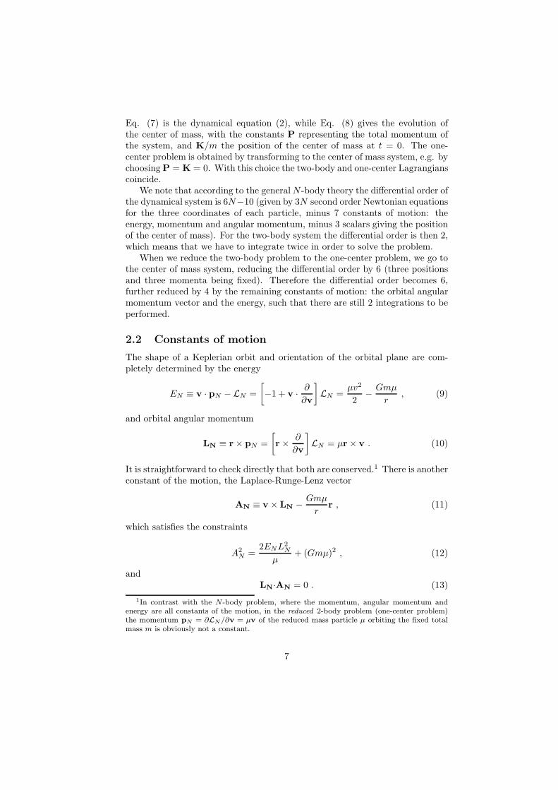
We note that according to the generalN -body theory the differential order ofthe dynamical system is 6N−10 (given by 3N second order Newtonian equationsfor the three coordinates of each particle, minus 7 constants of motion: theenergy, momentum and angular momentum, minus 3 scalars giving the positionof the center of mass). For the two-body system the differential order is then 2,which means that we have to integrate twice in order to solve the problem.
When we reduce the two-body problem to the one-center problem, we go tothe center of mass system, reducing the differential order by 6 (three positionsand three momenta being fixed). Therefore the differential order becomes 6,further reduced by 4 by the remaining constants of motion: the orbital angularmomentum vector and the energy, such that there are still 2 integrations to beperformed.
2.2 Constants of motion
The shape of a Keplerian orbit and orientation of the orbital plane are com-pletely determined by the energy
EN ≡ v · pN − LN =
[
−1 + v · ∂∂v
]
LN =µv2
2− Gmµ
r, (9)
and orbital angular momentum
LN ≡ r× pN =
[
r× ∂
∂v
]
LN = µr× v . (10)
It is straightforward to check directly that both are conserved.1 There is anotherconstant of the motion, the Laplace-Runge-Lenz vector
AN ≡ v × LN − Gmµ
rr , (11)
which satisfies the constraints
A2N =
2ENL2N
µ+ (Gmµ)2 , (12)
andLN·AN = 0 . (13)
1In contrast with the N-body problem, where the momentum, angular momentum andenergy are all constants of the motion, in the reduced 2-body problem (one-center problem)the momentum pN = ∂LN/∂v = µv of the reduced mass particle µ orbiting the fixed totalmass m is obviously not a constant.
7

Due to the constraint (12) only one of its components is independent of theother constants of motion EN ,LN. Thus there are five constants of motionaltogether, which means that there is one integration left in order to solve theproblem. Due to the constraint (13) the Laplace-Runge-Lenz vector lies in theplane of motion, determined by LN (the direction of LN). Its magnitude beingexpressed in terms of EN and LN , the only independent information carried byAN remains its orientation in the plane of the orbit.
2.3 The orbit
2.3.1 Parametrization of the radial motion by the true anomaly
As the orbital angular momentum is constant, the plane of motion is conserved.Eqs. (9) and (10) imply that Newtonian dynamics is determined by EN andLN , as encoded in the relations:
v2 =2ENµ
+2Gm
r, (14)
ψ =LNµr2
. (15)
Here ψ is the azimuthal angle in the fixed plane of motion. As consequence ofv2 = r2 + r2ψ2, a first order differential equation for the radial variable r (t)(the radial equation) is found:
r2 =2ENµ
+2Gm
r− L2
N
µ2r2. (16)
Eqs. (15) and (16) give
d(
GmµAN
− L2
N
µAN r
)
√
1−(
GmµAN
− L2
N
µAN r
)2= ±dψ , (17)
with the + (−) sign applying when r increases (decreases) in time. With thechange of variable
r =L2N
µ (Gmµ+AN cosχ), (18)
Eq. (17) becomes sgn (sinχ) dχ = ±dψ, solved for
χ = ψ − ψ0 , (19)
the true anomaly angle χ being 0 at the point of closest approach (the peri-astron), where the azimuthal angle is ψ0 and r = rmin. This choice gives thecorrect sign both when the point masses approach each other (at χ < 0), andwhen the separation increases (at χ > 0). The most distant point of the orbit isfound for χ = ±π if Gmµ ≥ AN (such that r stays positive). If the inequality is
8
strict, this represents the apastron and the orbit is bounded (r = rmax is finiteat χ = ±π ). For Gmµ = AN the orbit opens up with r → ∞, when χ → ±π.For Gmµ < AN the orbit becomes unbounded (r → ∞) already for certain χ±with |χ±| < π.
As discussed in Section 2.2, there are 5 constants of motion in the one-center problem, therefore the differential order is 6− 5 = 1. Although obtainedin an integration process, the expressions (18) and (19) represent only a newradial variable (which happens to be an angle), and we still have to performthe integration giving the complete solution of the problem. The remainingdifferential equation is Eq. (15). By employing the true anomaly, this can berewritten as the coupled system:
r =ANLN
sinχ , (20)
dt
dχ=
µ
LNr2 . (21)
Eq. (20) shows that there are turning points (r = 0) only at χ = 0,±π. Beforecarrying on the remaining integration, we discuss in more detail the Keplerianorbits.
2.3.2 Conics
The orbit r (ψ), as given by Eqs. (18) and (19), represents a conic section,the intersection of a plane with a cone. We can see this by introducing theparameter (semilatus rectum) and the eccentricity as
p =L2N
Gmµ2, (22)
e =ANGmµ
. (23)
Eq. (23) relates the magnitude of the Laplace-Runge-Lenz vector to the ec-centricity of the orbit. Due to the constraint (12) the eccentricity can be alsoexpressed in terms of EN , LN . According to our previous remarks, e ∈ [0, 1)characterizes bounded orbits, while e ≥ 1 is for unbounded orbits.
Eq. (18) becomes
r =p
1 + e cosχ. (24)
We can get further information on these orbits by rewriting the equation (24)into Cartesian coordinates x = r cosχ, y = r sinχ. We get:
(
1− e2)
x2 + y2 = p2 − 2epx , with ex < p . (25)
When x = 0, the above equation gives y = ±p, the points of intersection of theconic with the y-axis. There are four distinct classes of conics, distinguished by
9

the value of eccentricity. Eq. (25) describes:
a circle (e = 0): x2 + y2 = p2 , (26)
an ellipse (0 < e < 1):
(
x+ ep1−e2
)2
(
p1−e2
)2 +y2
(
p√1−e2
)2 = 1 , (27)
a parabola (e = 1): y2 = p2 − 2px , (28)
a hyperbola (e > 1):
(
epe2−1 − x
)2
(
pe2−1
)2 − y2(
p√e2−1
)2 = 1 . (29)
All these curves are represented in the center of mass system (see Fig. 1), theorigin being the focus of the conics.
The orbit with e = 0 represents a circle with radius p.The orbits with e ∈ (0, 1) are ellipses. Eq. (27) gives their semimajor and
semiminor axes as a = p/(
1− e2)
and b = p/√1− e2. The distances of the
apastron and periastron measured from the focus are found either from Eq.(24) for χ = π, 0 as rmax
min= p/ (1∓ e) = a (1± e) or from Eq. (27) for y = 0 as
x = ∓rmax
min. The distance between the focus and the center of symmetry of the
ellipse is a− rmin = ae (the linear eccentricity).For e = 1 Eq. (24) represents a parabola and for e ∈ (1,∞) a hyperbola.
Their point of closest approach to the focus is given by rmin = p/2 for theparabola and rmin = p/ (1 + e) for the hyperbola. Both are unbounded orbitswith limr→∞ χ = ±π for the parabola and limr→∞ χ = χ± = ± arccos (−1/e)for the hyperbola. This means that at infinity the two branches of the parabolabecome parallel (and horizontal), while the two branches of the hyperbolaasymptote to the directions χ±. For e → ∞ the hyperbola becomes a straightline, with χ∞
± = ±π/2. In analogy with the ellipse, for the hyperbola we define
a = p/(
e2 − 1)
and b = p/√e2 − 1. Then for both the ellipse and hyperbola
the parameter can be expressed as p = b2/a.By shifting horizontally all points of a conic with a distance which is e−1
times their distance from the focus, we obtain xd = e−1r+r cosχ = p/e =constant,which defines a vertical line, the directrix. The constant xd is also known asthe focal parameter. The focus, the directrix and the eccentricity represent anequivalent definition of the conics (the circle being an exception). For an ellipse,the distance between the symmetry center and the directrix is p/e+ ae = a/e.(The circular orbit limit p = a = b becomes degenerated: for a given radius andcenter the directrix is shifted to infinity; while for a given directrix and centerat finite separation the radius becomes zero.)
10

Figure 1: Circular (e = 0; brown), elliptic (e = 0.5; red), parabolic (e = 1;green), hyperbolic (e = 1.8; purple) orbits and the directrices for the ellipse,parabola and hyperbola, represented in the center of mass system (the origin isin the focus of the conics). The parameter (here p = 2) defines the intersectionpoints of the conics with the y-axis. While the circle and the ellipse run overthe whole allowed domain χ ∈ (−π, π], the parabola is depicted only for therange χ ∈ [−2.35, 2, 35] and the hyperbola for χ ∈ [−1.92, 1.92]. All representedorbits have the same orbital angular momentum, but different energyEcircularN <
EellipticN < EparabolicN = 0 < EhyperbolicN .
11

2.3.3 Dynamical characterization of the periastron
For non-circular orbits we introduce the following orthogonal basis in the planeof motion, constructed from the constants of motion:
AN = µ
(
2ENµ
+Gm
r
)
r−µrrv ,
QN = LN ×AN = Gmµ2rr+(
L2N −Gmµ2r
)
v . (30)
Thus for generic orbits the unit vectors
f(i)
= (AN, QN, LN) (31)
form a fixed orthonormal basis. The position and velocity vectors in this basisare:
r =1
µ
(
ρAN + σQN
)
, (32)
v = τAN + λQN , (33)
with coefficients
ρ =L2N −Gmµ2r
AN, σ =
LNAN
µrr ,
τ = −GmµAN
r , λ =LNAN
(
2ENµ
+Gm
r
)
. (34)
[We note that in terms of the coefficients (34): LN = ρλ− στ .]The coefficients (34) can be rewritten in terms of the true anomaly by using
Eqs. (12), (18), and (20):
ρ = µr cosχ , σ = µr sinχ ,
τ = −GmµLN
sinχ , λ =AN +Gmµ cosχ
LN. (35)
The position vector (32) thus becomes
r = r(
AN cosχ+ QN sinχ)
. (36)
At the turning point(s) of the radial motion the position vector is aligned withthe Laplace-Runge-Lenz vector: r = r cosχAN. At the periastron r (χ = 0) =rminAN, therefore we conclude that the Laplace-Runge-Lenz vector points to-ward the periastron.
The basis
r, LN × r
is related to the basis
AN, QN
by a rotation
with angle χ in the plane of motion, which is also obvious from the definition
12

of the true anomaly. In this basis in terms of the true anomaly the velocity isexpressed as
v =Gmµ
LN
[
−AN sinχ+ QN
(
cosχ+ANGmµ
)]
. (37)
In summary LN gives the plane of motion, two of the three dependent quan-tities (EN , LN , AN ) determine the shape of the orbit, finally AN indicates theposition of the periastron. This completes the characterization of the Keplerianorbit in terms of dynamical constraints.
2.4 Solution of the equations of motion: the Kepler equa-
tion
Eq. (21) can be rewritten as [see Eq. (72)]:
dt =2L3
N
(
1 + tan2 χ2)
d(
tan χ2
)
µ (Gmµ+AN )2(
1 + Gmµ−AN
Gmµ+ANtan2 χ2
)2 . (38)
We introduce y = tan (χ/2) as a new integration variable. There are three casesto consider, depending on the sign of (Gmµ−AN ). For circular or elliptic orbitsα = (Gmµ−AN ) / (Gmµ+AN ) ∈ (0, 1], for parabolic orbits Gmµ − AN = 0,while for hyperbolic orbits β ≡ −α = (AN −Gmµ) / (AN +Gmµ) ∈ (0, 1).Therefore in each case we evaluate one of the integrals:
∫
(
1 + y2)
dy
(1 + αy2)2 =
1 + α
2α3/2
[
arctan(α1/2y)− 1− α
1 + α
α1/2y
(1 + αy2)
]
, (39)
∫
(
1 + y2)
dy = y +1
3y3 , (40)
∫
(
1 + y2)
dy
(1− βy2)2 =
β − 1
2β3/2
[
arctanh(β1/2y)− 1 + β
1− β
β1/2y
(1− βy2)
]
. (41)
2.4.1 Circular and elliptic orbits
It is straightforward to introduce the variable
x =
√
Gmµ−ANGmµ+AN
tanχ
2, (42)
in terms of which [employing the result (39)] the remaining dynamical equation,Eq. (38) can be integrated as
t− t0 = 2Gm
(
µ
−2EN
)3/2 (
arctanx− ANGmµ
x
1 + x2
)
. (43)
13

With the change of variable
x = tanξ
2(44)
this gives the Kepler equation
t− t0 = Gm
(
µ
−2EN
)3/2(
ξ − ANGmµ
sin ξ
)
. (45)
The parameter ξ is the eccentric anomaly, and as can be seen from its definition,Eqs. (42) and (44) it passes through the values 0,±π,±2π, ... together with χ.From ξ = 0 to ξ = 2π the time elapsed is t − t0 = TN , thus we find the radialperiod
TN = 2πGm
(
µ
−2EN
)3/2
. (46)
2.4.2 Parabolic orbits
By employing Eq. (40), the equation (38) integrates as:
t− t0 =L3N
2G2m2µ3
(
tanχ
2+
1
3tan3
χ
2
)
. (47)
This is the analogue of the Kepler equation for parabolic orbits. The motionalong each branch takes infinite time: limχ→±π (t− t0) = ±∞.
2.4.3 Hyperbolic orbits
By employing Eq. (41) and introducing the variable
z =
√
AN −Gmµ
AN +Gmµtan
χ
2= ix , (48)
the equation (38) integrates as:
t− t0 = −2Gm
(
µ
2EN
)3/2(
arctanh z − ANGmµ
z
1− z2
)
. (49)
With the further change of variable
z = tanhζ
2(50)
we obtain the analogue of the Kepler equation for hyperbolic orbits:
t− t0 = −Gm(
µ
2EN
)3/2(
ζ − ANGmµ
sinh ζ
)
. (51)
14

periastron most distant pointrmin χmin ξmin rmax χmax ξmax
elliptic orbits a (1− e) 0 0 a (1 + e) ±π ±πparabolic orbits p
2 0 – ∞ ±π –hyperbolic orbits a (e− 1) 0 0 ∞ ± arccos
(
− 1e
)
−i (±∞)
Table 1: The values of the radial coordinates at the points of closest approachand maximal separation. The circular orbit limit arises at e→ 0 from the ellipticorbits, however for circular orbits the definition of these points is ambiguous.For parabolic orbits, the eccentric anomaly parametrization remains undefined.
Again, the travel time to χ± = ± arccos (−1/e) is infinite. In order to showthis, first we remark that
tanχ±2
= ±√
e+ 1
e− 1= ±
√
AN +Gmµ
AN −Gmµ, (52)
such that Eqs. (48) and (50) give ζ± = 2 arctanh (±1) = ±∞, irrespective ofthe value of eccentricity. Thus, limζ→ζ±=±∞ (t− t0) = ±∞.
Remarkably, the equation (51) can be obtained from the Kepler equation(45) derived for circular / elliptic orbits, by the substitution ξ → −iζ. Therelation between the variable ζ and the true anomaly χ also emerges from Eqs.(42) and (44) with the same substitution.
We summarize these in Table 2.4.3:
2.4.4 The eccentric anomaly: a summary
In the circular and elliptic case we have introduced the eccentric anomaly cf.:
tanξ
2=
√
Gmµ−ANGmµ+AN
tanχ
2. (53)
There is no parabolic limit for this equation, however it turned out that it canalso be employed in the hyperbolic case, with the change ξ → −iζ .
There is actually much simpler to obtain the Kepler equation, providedwe already define the eccentric anomaly before integration. Passing to the ξvariable in Eq. (18) by straightforward trigonometric transformations2 givesthe eccentric anomaly parametrization of the radial variable
r =Gmµ−AN cos ξ
−2EN. (54)
Taking its time derivative and employing Eq. (20) gives
−2ENLN
sinχ = ξ sin ξ . (55)
2The most quicker way would be to employ the forthcoming second relation (76).
15

Then with the help of Eq. (53) we eliminate χ and obtain:3
rξ =
(−2ENµ
)1/2
. (56)
With r (ξ) given by Eq. (54) and TN by Eq. (46) this becomes
2π
TN
dt
dξ= 1− AN
Gmµcos ξ , (57)
a relation, which immediately integrates to the Kepler equation (45). In thecircular and elliptic cases TN represents the orbital period.
In terms of the eccentric anomaly the radial motion and time are parametrizedthus as given by Eq. (54) and
nN (t− t0) = ξ − ANGmµ
sin ξ , (58)
where nN = 2π/TN is the mean motion and t0 an integration constant, the timeof periastron passage. It is also customary to quote the left hand side of theKepler equation (58) as the mean anomaly
MN = nN (t− t0) , (59)
and M0 = −nN t0 the mean anomaly at the epoch.Eqs. (54)-(58) are also valid for the hyperbolic case, with TN given by its
definition (46) and by replacing ξ → −iζ.
2.5 Orbital elements
When a reference plane (given on Fig. 2 by its normal z) and a reference axisx on it are given (these define an orthonormal reference basis), the orientationof the orbit can be characterized by three angles. The intersection of the planeof the orbit and the reference plane defines the node line. The angle subtendedby the plane of motion with the reference plane, ι (the inclination); the anglesubtended by the reference direction with the ascending node, Ω (the longitudeof the ascending node) and the angle between the ascending node and periastron,ω (the argument of the periastron) are the three angular orbital elements. Whenthe origin of time is chosen at the passage on the ascending node, ω = ψ0.Instead of ω sometimes the longitude of the periastron, ω = Ω+ ω is chosen.
The orthonormal basis (31) is expressed in the reference system in terms ofthe above angles (see Fig. 2) as:
(
AN
QN
)
=
(
cosω sinω− sinω cosω
)(
l
m
)
, (60)
LN =
sin ι sinΩ− sin ι cosΩ
cos ι
, (61)
3The most quicker way would be to employ the forthcoming first relation (76).
16

where the unit vectors
l =
cosΩsinΩ0
, m =
− cos ι sinΩcos ι cosΩ
sin ι
, (62)
point along the ascending node and perpendicular to it in the plane of the mo-tion, respectively. Therefore once the reference plane and direction are chosen,LN and AN are equivalent with the angles (ι, Ω) and ω, respectively.
A fourth orbital element is the time of periastron passage, t0. Alternativeoptions for the fourth orbital element are ε = ω +M0 (the mean longitude atthe epoch) and ε∗ = ε+ nN t−
∫
nNdt.The parameter p and eccentricity of the orbit e are the two remaining or-
bital elements. From Eqs. (12). (22), and (23) we can express the dynamicalconstraints as function of them:
L2N = Gmµ2p , (63)
AN = Gmµe , (64)
EN =Gmµ
(
e2 − 1)
2p, (65)
We see that for a given value of L2N (fixing the parameter), the circular, elliptical,
parabolic and elliptic orbits have the energies
EcircularN = −G
2m2µ3
2L2N
< 0 ,
EellipticN = −G
2m2µ3
2L2N
(
1− e2)
< 0 ,
EparabolicN = 0 ,
EhyperbolicN =
G2m2µ3
2L2N
(
e2 − 1)
> 0 , (66)
respectively. Thus for a given L2N , the energies of the orbits obey Ecircular
N <
EellipticN < Eparabolic
N = 0 < EhyperbolicN . In terms of dynamical constants
the circular orbits are characterized by AcircularN = 0, the parabolic orbits by
EparabolicN = 0.For elliptical and circular orbits the role of the parameter as an orbital
element can be taken by the semimajor axis a = p/(
1− e2)
. Eq. (65) thengives
Ecircular, ellipticN = −Gmµ
2a. (67)
2.6 Kinematical definition of the parametrizations for the
elliptic and parabolic motions
The parametrization of the orbits in the plane of motion relies on the knowledgeof their geometrical characteristics p and e. An alternative procedure, relying
17

Figure 2: The horizontal plane, defined by its normal z is the reference plane.On it, a reference direction x is chosen. The plane tilted with the angle ι (theinclination) is the plane of motion, defined by the vectors r, v, or equivalently byits normal LN. On the plane of motion three orthonormal bases are frequently
used. These are
r, LN × r
,
l, m = LN × l
and
AN, Q = LN × AN
,
where l and AN point along the ascending node (the intersection line of thetwo planes) and towards the periastron (the point of closest approach). Theazimuthal angle for l measured from x in the reference plane is Ω (the longitudeof the ascending node). The azimuthal angle for AN measured from l in theplane of motion is ω (the argument of the periastron). Note that the projectionof LN into the reference plane is also contained in the plane spanned by LN
and z. As both these vectors are perpendicular to l, so is the projection of LN.Therefore the azimuthal angle of LN measured from x in the reference plane isΩ−π/2, while its polar angle is ι. The azimuthal and polar angles of the vectorm are π/2 + Ω and π/2 − ι, respectively. Finally, the true anomaly χ is theazimuthal angle in the plane of motion of the position vector r.
18

on kinematics, would be much useful for generalizing to a perturbed Keplermotion. Such a description can be built from the knowledge of the turningpoint(s), defined as r = 0. This gives two turning points rmax
minfor the ellipse and
one turning point rmin for the parabola and hyperbola. Therefore a descriptionbased on the turning point(s) rather than (p, e) can be worked out for the ellipticand parabolic orbits (as the latter is characterized by p alone).
2.6.1 Elliptic orbits
For elliptic orbits an alternative way to find the solution (18) of the radialequation (16) is to follow the two steps:
(a.) determine the turning points rminmax
from the condition r = 0. To Newto-
nian order the solution is rmax
min
= r± given by
r± =L2N
µ(Gmµ∓AN )=Gmµ±AN
−2EN, (68)
(b1.) define the true anomaly parametrization as
2
r=
(
1
rmin+
1
rmax
)
+
(
1
rmin− 1
rmax
)
cosχ , (69)
Then it is straightforward to verify that Eqs. (18) and (21) hold.An equivalent form of the solution of the equations of motion can be given
in terms of the eccentric anomaly ξ, an alternative definition of which is(b2.)
2r = (rmax + rmin)− (rmax − rmin) cos ξ , (70)
It is immediate to verify that the following relation holding between the twoparametrizations is equivalent with the definition of ξ given in the precedingsubsection:
tanχ
2=
(
rmax
rmin
)1/2
tanξ
2. (71)
We also mention the follow-up relations:4
sinχ =2 (rminrmax)
1/2sin ξ
(rmax + rmin)− (rmax − rmin) cos ξ,
cosχ = − (rmax − rmin)− (rmax + rmin) cos ξ
(rmax + rmin)− (rmax − rmin) cos ξ. (74)
4These can be derived from the trigonometric relations
cosχ =1− tan2 χ
2
1 + tan2 χ
2
, sinχ =2 tan χ
2
1 + tan2 χ
2
, (72)
and their inverse (written for ξ)
tan2ξ
2=
1− cos ξ
1 + cos ξ, tan
ξ
2=
sin ξ
1 + cos ξ. (73)
19

This form of the true and eccentric anomaly parametrizations will be particu-larly suitable in discussing perturbed Keplerian orbits.
Eqs. (74) can be rewritten by employing Eq. (70) as
r sinχ = (rminrmax)1/2
sin ξ ,
2r cosχ = (rmax + rmin) cos ξ − (rmax − rmin) . (75)
The turning points rmaxmin
= r± being given by Eq. (68), we find (rminrmax)1/2
=
LN/ (−2µEN)1/2
, rmax + rmin = Gmµ/ (−EN ) and rmax − rmin = AN/ (−EN ).We obtain:
r sinχ =LN sin ξ
(−2µEN )1/2
,
r cosχ =Gmµ cos ξ −AN
−2EN. (76)
2.6.2 Parabolic orbits
The true anomaly parametrization (69) can be extended for this case. In thelimit rmax → ∞ it becomes
r =2rmin
1 + cosχ, (77)
in accordance with the conic equation (24) and the earlier remark p = 2rmin forthe parabola. Therefore the true anomaly parametrization can be used in thedescription of parabolic orbits.
20

3 The perturbed two-body system
The dynamical constants and orbital elements of the Keplerian motion slowlyvary due to perturbing forces. In this section we discuss this variation.
3.1 Lagrangian description of the perturbation
The motion of two bodies under the influence of generic perturbations can oftenbe characterized by a Lagrangian:
L (r,v, a, t) = LN (r,v) + ∆L (r,v, a, t) , (78)
where ∆L represents the collection of perturbation terms. We allow ∆L to beof second differential order (depending on coordinates, velocities and accelera-tions). The Euler-Lagrange equations in this case are:
(
∂
∂r− d
dt
∂
∂v+d2
dt2∂
∂a
)
L = 0 . (79)
We define the acceleration in the perturbed case as
a =1
µ
d
dt
∂
∂vLN . (80)
Remembering the definition of the Newtonian acceleration, Eq. (2) and with theremark that the Newtonian part of the Lagrangian is acceleration-independent,we can rewrite Eq. (79) as:
∆a ≡ a− aN =1
µ
(
∂
∂r− d
dt
∂
∂v+d2
dt2∂
∂a
)
∆L . (81)
The quantity ∆a is of the order of perturbations. Because of this, wheneveraccelerations or its derivatives appear when the right hand side of the aboveequation is evaluated, they can be replaced by the corresponding Newtonianexpressions.
3.2 Evolution of the Keplerian dynamical constants in
terms of the perturbing force
We decompose the sum of the perturbing forces per unit mass ∆a in the (slowlyevolving) basis fi as:
∆a =αAN + βQN + γLN . (82)
We can apply the forthcoming description of the perturbed Keplerian motionbased on the components α, β, γ even when a Lagrangian description is notavailable.
The Keplerian dynamical constants are not related to the symmetries of theperturbed dynamics, and are not constants of motion in general. Nevertheless,
21

they are useful in monitoring the evolution of the orbital elements, as will bediscussed later in this Section. In this subsection we wish to determine theirvariation as function of the components α, β, γ of the perturbing force.
The time derivative of Eq. (14) gives
EN = µv ·∆a . (83)
In the basis
f(i)
= (AN, QN, LN) it becomes:
EN = µ (τα+ λβ) , (84)
with the coefficients given in Eqs. (35). We note that the angle χ involved inthese coefficients is spanned by AN and r, as in the unperturbed case and willbe denoted χp in what follows.
The Newtonian orbital angular momentum evolves as:
LN = µr×∆a . (85)
In the chosen basis we find
LN = γ(
σAN − ρQN
)
+ (ρβ − σα) LN . (86)
Employing the generic formula for the time derivative of any vector V,
V =V V+Vd
dtV , (87)
both the evolution of the magnitude and of the direction of the Newtonianorbital angular momentum are found:
LN = ρβ − σα , (88)
d
dtLN =
γ
LN
(
ρAN + σQN
)
× LN = γµ
LNr× LN , (89)
The last equation describes the change of the orbital plane.The Laplace-Runge-Lenz vector also evolves in the presence of perturbations.
This can be seen by computing the time derivatives of Eq. (11) and recallingthat AN is a constant of the Keplerian motion:
AN = ∆a × LN + v × LN
= µ [2 (v·∆a) r− (r·∆a)v− (r · v)∆a] . (90)
Computation gives
AN=(
βLN + λLN
)
AN −(
αLN + τLN
)
QN − γ (τρ+ λσ) LN , (91)
from which we identify
AN = βLN + λLN , (92)
d
dtAN =
1
AN
[
γ (τρ+ λσ) QN −(
αLN + τLN
)
LN
]
× AN , (93)
22

The last equation describes the evolution of the periastron, composed from aprecessional part in the plane of the motion (about LN) and a coevolution withthe plane of motion.
With the expression of the coefficients (35) the evolution of EN , LN andAN are obtained explicitly as:
EN = −αGmµ2
LNsinχp + β
µ (AN +Gmµ cosχp)
LN,
LN = µr (β cosχp − α sinχp) ,
AN = βLN +AN +Gmµ cosχp
LNµr (β cosχp − α sinχp) . (94)
Note that the time derivative of Eq. (12) gives an identity with the aboveevolutions and employing the true anomaly parametrization (18), therefore thealgebraic relation (12) continue to hold in the perturbed case.
The evolution of AN and LN will be given in explicit form in the nextsubsection.
3.3 Precession of the basis vectors in terms of the per-
turbing force
As a by-product of the calculations of the subsection 3.2, we also obtained theprecession of two of the basis vectors
f(i)
. The precession of the remaining
basis vector of the basis
f(i)
can be derived from its definition QN = LN×AN.
d
dtQN =
[
γρ
LNAN − αLN + τLN
ANLN
]
× QN . (95)
Inserting the explicit expression (35) for the coefficients ρ, σ, τ, λ (with χp inplace of χ) in the Eqs. (89), (93) and (95) we obtain the explicit expressions ofthe precessional motion of the basis vectors (31):
f(i) = Ω(i) × f(i) , (96)
with
Ω(1) = γµr sinχpLN
QN
−[
αLNAN
+ (α sinχp − β cosχp)Gmµ2r sinχpLN AN
]
LN , (97)
Ω(2) = γµr cosχpLN
AN
−[
αLNAN
+ (α sinχp − β cosχp)Gmµ2r sinχpLN AN
]
LN , (98)
Ω(3) = γµr cosχpLN
AN + γµr sinχpLN
QN , (99)
23

As f(i)× f(i) = 0, we can add to the above expressions of Ω(i) terms proportionalto f(i), such that we have a single angular velocity vector Ω, with components
in the
f(i)
basis:
Ωj =
(
γµr cosχpLN
, γµr sinχpLN
,−[
αLNAN
+ (α sinχp−β cosχp)Gmµ2r sinχp
LNAN
])
.
(100)Then
f(i) = Ω× f(i) . (101)
The expressions (83)-(100) manifestly vanish in the Newtonian limit togetherwith either ∆a or the coefficients α, β and γ.
A couple of immediate remarks are in order:(a) If γ = 0 (no perturbing force is pointing outside the plane of motion),
LN (the plane of motion) is conserved, while both AN and QN undergo aprecessional motion about LN (in the conserved plane of motion).
(b) If α = β = 0 (the perturbing force is perpendicular to the plane ofmotion), then AN undergoes a precessional motion about QN and vice-versa,while LN about r.
3.4 Summary
The perturbed bounded Keplerian motion can be visualized as a Keplerianellipse with slowly varying parameters. The semimajor axis a and eccentricity ecan be defined exactly as in the unperturbed case, from the dynamical quantitiesEN and AN . The evolution of a, e can be inferred then from the evolutions ofEN , AN . The orbit therefore rather of being an exact ellipse should be thoughtof as a curve which can be approximated in each of its points by an ellipse withthese slowly varying parameters a, e. This description is known as an osculatingellipse.
Whenever the force depends on χp only, the evolution equations (94) (sup-plemented with the additional evolution equations of any dynamical variable- like the spins - possibly contained in α, β) give the radial evolution of thebinary system (provided an equation dt/dχp holding in the perturbed case isprovided - this will be given in chapter 5.1). The additional equations (89) and(93) give the angular evolutions, e.g. the evolution of the orbital plane and ofthe precession of the periastron in the orbital plane.
The equations (84), (89), (92) and (93) are equivalent with the Lagrangeplanetary equations for the orbital elements (a, e, ι,Ω, ω) of the osculating orbit,as will be shown in the next section. However the use of the above mentionedsystem of equations has the undoubted advantage of being independent of thechoice of the reference plane and axis.
24
4 The Lagrange planetary equations
In chapter 3 we have discussed in detail the evolution of a perturbed Kepleriansystem, relying on the corresponding evolution of the Keplerian dynamical con-stants. An alternative approach to this problem is represented by the Lagrangeplanetary equations. In this section we prove that they are equivalent to theevolution equations of the dynamical constants.
4.1 Evolution of the orbital elements in terms of the evo-
lution of Keplerian dynamical constants
We have seen that in the presence of perturbations the Keplerian dynamicalconstants EN , LN and AN slowly vary. Due to perturbations a related slowevolution of the orbital elements also occurs. In this subsection we determinethe latter as function of the former.
From Eqs. (63) and (64) we find
LN =[
Gmµ2a(1− e2)]1/2
×[(
a
2a− ee
1− e2
)
LN +d
dtLN
]
, (102)
AN = Gmµ
(
eAN + ed
dtAN
)
(103)
The time-derivatives of Eqs. (61)-(62) give generic expressions for the time-derivatives of l, m and LN in terms of the time-derivatives of the angular orbitalelements:
d
dtl = Ω
(
cos ι m− sin ι LN
)
, (104)
d
dtm = ι LN − Ω cos ι l , (105)
d
dtLN = −ι m+ Ω sin ι l , (106)
From these and the time derivatives of Eqs. (60) we obtain:
d
dtAN =
(
ω + Ω cos ι)
QN
+(
ι sinω − Ω sin ι cosω)
LN , (107)
d
dtQN = −
(
ω + Ω cos ι)
AN
+(
ι cosω + Ω sin ι sinω)
LN . (108)
Then the projections of the Eqs. (102)-(103) give the time derivatives of 5orbital elements as functions of the time derivatives of the Keplerian dynamical
25
constants:
ι = − LN · m[Gmµ2a(1− e2)]1/2
, (109)
Ω =LN · l
[Gmµ2a(1 − e2)]1/2
sin ι, (110)
ω =AN · QN
Gmµe−
(
LN · l)
cot ι
[Gmµ2a(1 − e2)]1/2
, (111)
a = 2a
LN · LN
[Gmµ2a(1− e2)]1/2
+e(
AN · AN
)
Gmµ (1− e2)
, (112)
e =AN · AN
Gmµ. (113)
4.2 Evolution of the orbital elements in terms of the per-
turbing force
Based on the expressions
LN = LNΩ2AN − LNΩ1QN + LN LN , (114)
AN = AN AN +ANΩ3QN −ANΩ2LN , (115)
with the coefficients derived in the previous section, the relations (60) betweenthe basis vectors in the plane of motion, and on Eqs. (63) and (64) giving LNand AN in terms of orbital elements, the variation (109)-(113) of the orbitalelements can be expressed in terms of the perturbing force components as:
ι = Ω1 cosω − Ω2 sinω , (116)
Ω =Ω2 cosω +Ω1 sinω
sin ι, (117)
ω = Ω3 − (Ω2 cosω +Ω1 sinω) cot ι , (118)
a = 2a
[
LN
[Gmµ2a(1− e2)]1/2
+eAN
Gmµ (1− e2)
]
, (119)
e =ANGmµ
. (120)
From the above relations and the expression of the angular velocities (100) onereadily finds that
Ω = ιtan (ω + χp)
sin ι. (121)
26

The expressions giving the variation of the angular orbital elements can begiven explicitly by inserting the corresponding elements of the angular velocities(100) and employing Eq. (18) given in terms of the orbital elements as
r =a(
1− e2)
1 + e cosχp, (122)
together with Eq. (63). We obtain:
ι = γ
[
a(
1− e2)
Gm
]1/2cos (ω + χp)
1 + e cosχp, (123)
Ω = γ
[
a(
1− e2)
Gm
]1/2sin (ω + χp)
sin ι (1 + e cosχp), (124)
ω = −[
a(
1− e2)
Gm
]1/2
×α(
1+e cosχp+sin2 χp)
−β sinχp cosχp+γe cot ι sin (ω+χp)e (1 + e cosχp)
.(125)
Thus the angular orbital elements ι and Ω are changed only by perturbing forcesperpendicular to the plane of motion, while ω is changed by any perturbingforce. If the perturbing force is such that the plane of motion is unchanged(γ = 0), then l is also unaffected, and the change in ω can be interpreted aspure periastron precession: ω = Ω3 and ∆ω = ∆ψ0. (Otherwise stated γ = 0implies Ω1 = Ω2 = 0.)
Note that the α, β-parts of ω become ill-defined in the limit e→ 0. This ishowever not surprising, as ω cannot be defined for circular orbits.
The expressions (119)-(120) can be further expanded by employing Eqs.(94), obtaining
a =2a3/2
[Gm (1− e2)]1/2
[β (e+ cosχp)− α sinχp] , (126)
e =
[
a(1− e2)
Gm
]1/2 β(
1+2e cosχp+cos2 χp)
−α (e+cosχp) sinχp
1 + e cosχp.(127)
Thus the orbital elements a, e are not changed by perturbing forces perpendic-ular to the plane of motion.
Eqs. (123)-(125) and (126)-(127) are the Lagrange planetary equations.
27

5 Orbital evolution under perturbations in terms
of the true anomaly
In this section we return to the characterization of the orbit and dynamics interms of the dynamical constants of the Keplerian motion. Although the La-grange planetary equations are widely used, we find more convenient to discussthe perturbed Keplerian problem based on the equivalent set of equations (84),(89), (92) and (93), derived earlier in the subsection 3.2.
5.1 The perturbed Newtonian dynamical constants
As the basis
f(i)
is comoving with the plane of motion and the periastron, theposition vector
r = xif(i) (128)
with components
x1 = r cosχp, x2 = r sinχp, x3 = 0 (129)
changes according to (see also Appendix A)
v = xif(i) + xi f(i) = xif(i) + xiΩ× f(i)
=(
xi − ǫi kj xjΩk
)
f(i) , (130)
where ǫi kj is the antisymmetric Levi-Civita symbol and xi are found as the timederivatives of the coordinates (129).
Then, starting from the definition of the Newtonian orbital angular mo-mentum, Eq. (61), and employing the relations (128)-(130) and the angularvelocities (100), we obtain by straightforward algebra (see Appendix A)
LN = µr2 (χp +Ω3) LN . (131)
This reduces to the manifestly Newtonian expression, whenever Ω3 = 0 , thuswhenever AN does not precess about LN.
Similarly, starting from the definition of the energy, Eq. (9), by the samemethod (see Appendix A) we obtain
EN =µ(
r2 + r2χ2p
)
2− Gmµ
r+ µr2χp Ω3 +
µr2
2Ω2
3 . (132)
(The last O(
α2, αβ, β2)
term can be dropped in a linear approximation.)Again, whenever Ω3 = 0 , the Newtonian expression is recovered.
Therefore the Newtonian energy and Newtonian angular momentum sharethe properties, that modulo Ω3 terms they reduce to manifestly Newtonian
28

forms. We can express χp from Eq. (131) as5
χp =LNµr2
− Ω3 . (134)
Inserting this to Eq. (132), we obtain the radial equation
r2 =2ENµ
+2Gm
r− L2
N
µ2r2. (135)
Finally, starting from the definition of the Laplace-Runge-Lenz vector, Eq.(11) and employing the relations (128)-(130) and (131), we can deduce (seeAppendix A) its evolution as
AN =[
µr2χp (r sinχp + rχp cosχp)−Gmµ cosχp
+ µr2Ω3 (r sinχp + 2rχp cosχp + rΩ3 cosχp)]
AN
−[
µr2χp (r cosχp − rχp sinχp) +Gmµ sinχp
+ µr2Ω3 (r cosχp − 2rχp sinχp − Ω3r sinχp)]
QN . (136)
By inserting in the above relation χp given by Eq. (134), all Ω3 terms cancelout and we obtain:
AN =
[(
L2N
µr−Gmµ
)
cosχp + LN r sinχp
]
AN
+
[(
L2N
µr−Gmµ
)
sinχp − LN r cosχp
]
QN . (137)
As AN = ANAN:
AN =
(
L2N
µr−Gmµ
)
cosχp + LN r sinχp , (138)
0 =
(
L2N
µr−Gmµ
)
sinχp − LN r cosχp . (139)
Solving for r and r gives
L2N
µr−Gmµ = AN cosχp ,
LN r = AN sinχp . (140)
The derived expressions r (χp) and r (χp) are identical with the zeroth ordertrue anomaly parametrization r (χ) and zeroth order expression of r (χ), Eqs.
5This also arises from the relation
ω + χp =LN
µr2− Ω cos ι (133)
derived in Ref. [1], after inserting the relations (117) and (118).
29

(18) and (20), respectively. Therefore the true anomaly parametrization χp isintroduced exactly in the same way than in the unperturbed case.
As a consistency check, we calculate the derivative of r (χp) as
r =µANr
2χp sinχpL2N
+2rLNLN
− µr2AN cosχpL2N
, (141)
and put it equal to r (χp), derived earlier. We insert χp as given by Eq. (134);
also LN and AN as given by the Eqs (94). As a result, we re-obtain the expres-sion of Ω3 given in Eq. (100).
A second consistency check involving r (χp), r (χp) and the radial equation(135) also holds, as in the Keplerian motion.
5.2 The evolution of the Newtonian dynamical constants
in terms of the true anomaly
The scalars EN , LN , AN become χp-dependent in the presence of a perturb-ing force. We can decompose these Newtonian expressions in the unperturbed(Keplerian) part, and a χp-dependent correction as EN = E0
N + E1N (χp),
LN = L0N + L1
N (χp), AN = A0N + A1
N (χp). Their explicit expression canbe derived starting from their evolution equations (94), by passing from time-derivatives to derivatives with respect to χp. As all terms in the equations arefirst order, we simply employ χp = L0
N/µr2 and obtain:
dE1N
dχp=
Gmµ3
(L0N)
2 r2
[
−α sinχp + β
(
A0N
Gmµ+ cosχp
)]
,
dL1N
dχp=
µ2
L0N
r3 (β cosχp − α sinχp) ,
dA1N
dχp= µβr2 +
Gmµ3
(L0N)
2 r3 (β cosχp − α sinχp)
(
A0N
Gmµ+ cosχp
)
.(142)
By inserting r (χp) =(
L0N
)2/µ(
Gmµ+A0N cosχp
)
and provided the compo-nents of the perturbing force can be given as functions of χp alone (that is, theycan possibly depend on r and χp only), Eqs. (142) become ordinary differentialequations for E1
N , L1N and A1
N . Unless α, β ∝ rn≤−3 however, the integrals maybe cumbersome to evaluate due to the negative powers of
(
Gmµ+A0N cosχp
)
inthe integrands. In these cases the use of the eccentric anomaly parametrizationmay simplify the calculations (similarly as in the derivation of the unperturbedKepler equation). Therefore in the next section we will work out the details ofthis parametrization applying for the perturbed case.
5.3 Summary of the results obtained with the true anomaly
parametrization
The forces perturbing the Keplerian orbit do not change the true anomalyparametrization r (χp) and r (χp), Eqs. Eq. (18) and (20), respectively, with χp
30

in place of χ. In the order of accuracy of the perturbations the radial equation(16) also holds. These in turn mean that the eccentric anomaly parametriza-tion ξp can be introduced exactly as in the Keplerian case. We can also definea radial period as the time in which the mass µ moves from an rmin locationgiven by r = 0 to the following rmin, given by the second forthcoming r = 0locus (the first will give rmax).
The following, however are changed with respect to the Keplerian case:(a) The basis
f(i)
constructed from the Keplerian dynamical constantsslowly evolves, with precessional angular velocities Ωj given as linear and ho-mogeneous expressions of the components of the resulting perturbing force.
(b) The plane of motion, determined by LN, can change due to perturbationforces transverse to the plane of motion.
(c) The periastron, determined by AN, undergoes a composed evolution. Ithas a precession in the plane of motion due to the forces acting in the planeof motion (this is characterized by Ω3, the precessional angular velocity of AN
about LN) and it also moves with the plane of motion.(d) The precession of the periastron means that the orbit fails to be closed.
The χp-dependence of the Ω3 angular velocity component signifies that at eachmoment the movement of the periastron of the corresponding osculating ellipsewill be different. The change of AN over one radial period will give the perias-tron shift.
(e) When expressed in terms of the true anomaly χp, both the Newtonian or-bital angular momentum vector and the Newtonian energy acquire linear termsin Ω3, given in Eqs. (131) and (132), respectively.
(f) The scalars EN , LN , AN evolve in χp (or equivalently, in ξp).(g) The expression χp (r) is changed as compared to the corresponding Ke-
plerian expression by a linear term in Ω3 [Eq. (134)].
31

6 Orbital evolution under perturbations in terms
of the eccentric anomaly
In this section, besides rewriting all results of the previous section in terms ofthe eccentric anomaly, we derive the perturbed Kepler equation.
6.1 The eccentric anomaly parametrization
We introduce the eccentric anomaly parametrization similarly as in the Keple-rian case [by Eq. (54), with ξp in place of ξ]:
r =Gmµ−AN cos ξp
−2EN. (143)
From the expressions of r (χp) [given by the second relation (140) and em-ploying Eq. (76)], and of χp [given by Eqs. (134) and the third component ofthe expression (100)] we obtain r and χp in terms of the eccentric anomaly:
r =AN
(−2µEN)1/2
rsin ξp , (144)
rχp =LNµr
+ αLNAN
(
r +Gmµ
−2ENsin2 ξp
)
−β(
µ
−2EN
)1/2Gmµ
−2ENAN(Gmµ cos ξp −AN ) sin ξp . (145)
Similarly, the evolutions EN , LN and AN [given by Eqs. (94)], can be rewrittenin terms of ξp [by making use of the relations (12), (76) and (143)]:
rEN = −αGmµ(
µ
−2EN
)1/2
sin ξp + βLN cos ξp ,
LN = βµ (Gmµ cos ξp −AN )
−2EN− αLN
(
µ
−2EN
)1/2
sin ξp ,
AN = βLN +LNr
(
βGmµ cos ξp −AN
−2EN− α
LN sin ξp
(−2µEN)1/2
)
cos ξp .(146)
6.2 The evolution of the eccentric anomaly
In order to derive the perturbed Kepler equation for a given perturbing forcewith components α, β, γ, we need the expression of ξp to first order accuracy.This can be found, following the logic of the derivation in the Keplerian casefrom subsection 2.4.4.
By taking the time derivative of Eq. (143)
−2EN r − 2ENr = −AN cos ξp +AN ξp sin ξp . (147)
32

next employing the expressions (144) and (146) we obtain the desired relation
rξp =
(−2ENµ
)1/2
+ βGmµLN2ENAN
sin ξp cos ξp
+α
(−2ENµ
)1/2µ
AN
[
r2 +
(
Gmµ
−2EN
)2
sin2 ξp
]
. (148)
Another way of deriving this would be to start from the time derivative ofthe first Eq. (76), from which we eliminate sinχp and cosχp by use of the sameEqs. (76), to obtain
ξp cos ξp =
(
r
r− LNLN
+EN2EN
)
sin ξp
+
(
µ
−2EN
)1/2Gmµ cos ξp −AN
LNχp . (149)
Next we employ once again the expressions (144)-(146) and we recover therelation (148).
6.3 The evolution of the Newtonian dynamical constants
for ξp-dependent perturbing forces
By employing the eccentric anomaly parametrization for r, Eq. (143), the evolu-tion of Eqs. (146) in time can be rewritten as evolution in ξp, with dt = ξ−1
p dξp,
and ξp given by Eq. (148). We also take EN = E0N + E1
N (ξp) , AN =A0N + A1
N (ξp) , LN = L0N + L1
N (ξp), the zeroth order terms being the con-stant Keplerian values. As all terms in Eqs. (146) are first order, we canemploy the Newtonian expression of ξp [the leading order term in Eq. (148),
ξp = (−2EN/µ)1/2
/r]. We can also insert the constant values EN = E0N , AN =
A0N , LN = L0
N , in the manifestly first order terms. We obtain:
(−2E0N
µ
)1/2dE1
N
dξp= −αGmµ
(
µ
−2E0N
)1/2
sin ξp + βL0N cos ξp ,
(−2E0N
µ
)1/2dL1
N
dξp= r
[
βµ(
Gmµ cos ξp −A0N
)
−2E0N
− αL0N
(
µ
−2E0N
)1/2
sin ξp
]
,
(−2E0N
µ
)1/2dA1
N
dξp= βL0
Nr
+L0N
(
βGmµ cos ξp −A0
N
−2E0N
−α L0N sin ξp
(−2µE0N)
1/2
)
cos ξp .(150)
Here r should be replaced by its expression (143), taken only to zeroth orderaccuracy, as it is everywhere multiplied by the components of the perturbing
33

force. Provided the perturbing force components α, β can be expressed in termsof ξp alone, the above equations become ordinary differential equations, whichformally integrate to
EN = E0N − T 0
N
π
E0N
Gmµ
(
T 0N
πE0NIαs + L0
NIβc
)
, (151)
LN = L0N +
T 0N
2π
µ
2E0N
[
A0N
(
Iβ + Iβc2)
− (Gmµ)2+(
A0N
)2
GmµIβc
]
+T 0N
π
E0NL
0N
Gmµ
(
Iαs −A0N
GmµIαsc
)
, (152)
AN = A0N + L0
N
[
L0N
2E0N
Iαsc +T 0N
2π
(
Iβ + Iβc2 − 2A0N
GmµIβc
)]
. (153)
with
Iαs =
∫
α sin ξpdξp ,
Iαsc =
∫
α sin ξp cos ξpdξp ,
Iβ =
∫
βdξp ,
Iβc =
∫
β cos ξpdξp ,
Iβc2 =
∫
β cos2 ξpdξp . (154)
The notation was somewhat simplified by introducing the period T 0N of the
unperturbed motion, defined by Eq. (46) in terms of E0N . As a consistency
check, one can verify, that provided Eq. (12) holds for the Keplerian constantsE0N , L
0N , A
0N it will also hold for the values given in Eqs. (151)-(153).
From Eq. (151), by performing a series expansion in the small quantitiesIαs and Iβc, we can also write the expression of the period TN (of the Keplerianmotion on the osculating ellipse), defined in terms of EN in the same way asT 0N in terms of E0
N :
TN = T 0N
[
1 +3T 0
N
2πGmµ
(
T 0N
πE0NIαs + L0
NIβc
)]
. (155)
6.3.1 A note on the circularity of the perturbed orbit
In order the perturbed orbit to be circular (in the plane of motion, which canevolve due to γ), the eccentricity derived from AN = Gmµe should vanish.Therefore
L0N
−2E0N
Iαsc +T 0N
2π
(
2A0N
GmµIβc − Iβ − Iβc2
)
=A0N
L0N
(156)
34

should hold. If we further want the unperturbed orbit to be also circular, thenA0N = 0, such that
L0N
−2E0N
Iαsc =T 0N
2π
(
Iβ + Iβc2)
. (157)
Obviously, this is a condition very few perturbing forces would obey. Also, thecircularity of the perturbed orbit should be understood in a broad sense: whilecondition (156) holds the plane of motion could still undergo a precessionalmotion.
6.4 The Kepler equation in the presence of perturbations
By formally integrating Eq. (148), we obtain the perturbed Kepler equation.We first rewrite Eq. (148), by employing a series expansion in the small
parameters α and β as
dt
dξp= r
(
µ
−2EN
)1/2
1 + β
(
µ
−2EN
)3/2GmLNAN
sin ξp cos ξp
−α µ
AN
[
r2 +
(
Gmµ
−2EN
)2
sin2 ξp
]
. (158)
Next we insert the eccentric anomaly parametrization r (ξp), Eq. (143) andobtain:
dt
dξp=
TN2π
(
1− ANGmµ
cos ξp
)
1 + βTN2π
LNAN
sin ξp cos ξp
+ α
(
TN2π
)22ENAN
[
(
1− ANGmµ
cos ξp
)2
+ sin2 ξp
]
. (159)
In order to simplify the notation, here we have employed again the definitionof the Keplerian period, Eq. (46). In the perturbative terms the quantitiesTN , EN , LN , AN can be considered constants and replaced by their unper-turbed values, however for the leading order term we need the evolutions ofAN (ξp) and TN (ξp), given by Eqs. (153) and (155).
35

The Kepler equation is given then by the integral of Eq. (159):
2π
T 0N
(t− t0) = ξp −A0N
Gmµsin ξp −
(
L0N
)2
2GmµE0N
∫
Iαsc cos ξpdξp
+
(
T 0N
2π
)26E0
N
Gmµ
(∫
Iαsdξp −A0N
Gmµ
∫
Iαs cos ξpdξp
)
+T 0N
2π
L0N
Gmµ
[
3
∫
Iβcdξp −∫ (
Iβ + Iβc2 +A0N
GmµIβc
)
cos ξpdξp
]
+T 0N
2π
L0N
A0N
(
Iβsc −A0N
GmµIβsc2
)
+
(
T 0N
2π
)22E0
N
A0N
2Iα − 4A0N
GmµIαc
−[
1− 3
(
A0N
Gmµ
)2]
Iαc2 +A0N
Gmµ
[
1−(
A0N
Gmµ
)2]
Iαc3
. (160)
with
Iα =
∫
αdξp ,
Iαc =
∫
α cos ξpdξp ,
Iαc2 =
∫
α cos2 ξpdξp ,
Iαc3 =
∫
α cos3 ξpdξp ,
Iβsc =
∫
β sin ξp cos ξpdξp ,
Iβsc2 =
∫
β sin ξp cos2 ξpdξp (161)
As the integrations were formally carried out, the perturbed Kepler equation
36

(160) can be rewritten in terms of TN , EN , LN , AN :
2π
TN(t− t0) = ξp −
ANGmµ
sin ξp +LN
2Gmµ
[
LNEN
Iαsc
+3
(
TNπ
)2ENLN
ANGmµ
Iαs +TNπ
(
Iβ + Iβc2 +ANGmµ
Iβc
)
]
sin ξp
− 3TN2πGmµ
(
TNπENIαs + LNIβc
)
ξp −L2N
2GmµEN
∫
Iαsc cos ξpdξp
+
(
TN2π
)26ENGmµ
(∫
Iαsdξp −ANGmµ
∫
Iαs cos ξpdξp
)
+TN2π
LNGmµ
[
3
∫
Iβcdξp −∫ (
Iβ + Iβc2 +ANGmµ
Iβc
)
cos ξpdξp
]
+TN2π
LNAN
(
Iβsc −ANGmµ
Iβsc2
)
+
(
TN2π
)22ENAN
2Iα − 4ANGmµ
Iαc
−[
1− 3
(
ANGmµ
)2]
Iαc2 +ANGmµ
[
1−(
ANGmµ
)2]
Iαc3
. (162)
In order to evaluate the integrals appearing in either form of the Kepler equa-tion, we need the explicit time-dependence of the perturbing force components,α and β. Examples for this will be discussed in the forthcoming sections.
We also note, that the constants of integration should be chosen in such away, that the perturbative terms in the expressions of EN , LN , AN , TN [givenby Eqs. (151)-(153), (155)] and in either form of the Kepler equation [Eqs.(160), (162)] vanish at ξp = 0. In practice this means that all integrals (154),(161) should vanish at ξp = 0.
6.4.1 The radial period
In the perturbed two-body problem we define the radial period T of the per-turbed motion as double the time elapsed between successive passages throughpoints characterized by r = 0. From Eqs. (144) we see that r = 0 is equiv-alent to ξp = 0,±π,±2π, etc., therefore the radial period is obtained as T =∫ 2π
0t (ξp) dξp, or more simply, by inserting ξp = 2π in the perturbed Kepler
equation derived in the previous subsection. We note that T 6= TN |ξp=2π (the
latter representing the radial period on the osculating ellipse at 2π).
6.5 Summary
In the present and the previous chapters we have developed the formalism suit-able to describe the perturbed two-body problem. We have given explicit ex-pressions in the parameter ξp for the dynamical constants of the osculatingellipse EN and AN [Eqs. (151) and (153)], which define the semimajor axis andthe eccentricity of the osculating ellipse. The position of the osculating ellipse
37

in the plane of motion is characterized by the precession of AN about LN, orΩ3 (χp) [see its expression in Eq. (100), which can be rewritten in terms of ξpif required]. Finally, the plane of motion is given by LN, precessing about r [cf.Eq. (88)] in the case when the perturbing force has a component perpendicularto the plane of motion. As both precessions are first order effects, the directionsabout which the basis vectors precess, can be considered constants, defined bythe unperturbed dynamics.
The dynamics of the perturbed two-body problem is entirely contained inthe perturbed Kepler equation [in either of its forms (160) and (162)].
In the forthcoming chapters we will present some applications of the devel-oped formalism.
38

7 Constant perturbing force
In this section we present an application of the true and eccentric anomalyparametrizations of the perturbed Keplerian motion. We consider boundedorbits only. In the computationally simplest toy model presented here the per-turbing force is supposed to be constant on the orbit.
7.1 The evolution of the dynamical constants and of the
radial period
The integrals (154), (161) become:
Iα = αξp ,
Iαc = α sin ξp ,
Iαc2 =α
4(2ξp + sin 2ξp) ,
Iαc3 =α
12(sin 3ξp + 9 sin ξp) ,
Iαs = α (1− cos ξp) ,
Iαsc =α
4(1− cos 2ξp) ,
Iαsc2 =α
12(4− 3 cos ξp − cos 3ξp) . (163)
The constants of integration were chosen such that at ξp = 0 all these integralsvanish. Similar relations hold for the corresponding integrals containing β.
The expressions (151)-(153), (155) give for the perturbed valuesEN , LN , AN , TN :
EN = E0N − T 0
N
π
E0N
Gmµ
(
αT 0N
πE0N (1− cos ξp) + βL0
N sin ξp
)
, (164)
LN = L0N +
T 0N
2π
αT 0N
π
E0NL
0N
4Gmµ
(
4− A0N
Gmµ− 4 cos ξp +
A0N
Gmµcos 2ξp
)
+βµA0
N
8E0N
[
6ξp −4Gmµ
A0N
[
1 +
(
A0N
Gmµ
)2]
sin ξp + sin 2ξp
]
, (165)
AN = A0N +
L0N
8
[
αL0N
E0N
(1− cos 2ξp)
+βT 0N
π
(
6ξp −8A0
N
Gmµsin ξp + sin 2ξp
)]
, (166)
TN = T 0N
[
1 +3T 0
N
2πGmµ
(
αT 0N
πE0N (1− cos ξp) + βL0
N sin ξp
)]
. (167)
At ξp = 0 they take the initial values E0N , L
0N , A
0N , T
0N . Therefore, as a result
of our choice of the integration constants, these unperturbed values characterizethe osculating ellipse at the periastron.
39
By employing the relations (76) and (18) we find to leading order
cos ξp =AN +Gmµ cosχpGmµ+AN cosχp
,
sin ξp =
(
−2ENµ
)1/2LN sinχp
Gmµ+AN cosχp, (168)
which allow to rewrite EN , LN , AN , TN in terms of the true anomaly χp.However the emerging expressions are more complicated than Eqs. (164)-(167).
7.1.1 Changes and averages over one radial period
We define the change of a quantity f (ξp) over a radial period by ∆f (ξp) =f (ξp + 2π)− f (ξp). Such a change will be called a secular effect. Over a radialperiod we find
∆EN (ξp) = ∆TN (ξp) = 0 , (169)
∆LN = βT 0N
3µA0N
4E0N
, (170)
∆AN = βT 0N
3L0N
2. (171)
(The computation is very simple by realizing that we can drop all periodic andconstant terms.)
We define the average of a quantity f (ξp) over a radial period in the param-
eter ξp as fξ= (1/2π)
∫ 2π
0 f (ξp) dξp. We find:
ENξ
= E0N
[
1− α
(
T 0N
π
)2E0N
Gmµ
]
,
LNξ
= L0N
1 +T 0N
2π
[
αT 0N
π
E0N
4Gmµ
(
4− ANGmµ
)
+ β3πµA0
N
4E0NL
0N
]
,
ANξ
= A0N
[
1 +L0N
8A0N
(
αL0N
E0N
+ 6βT 0N
)]
,
TNξ
= T 0N
[
1 + α3E0
N
2Gmµ
(
T 0N
π
)2]
. (172)
Note that due to the secular contributions in β the definition above assures acorrect average only for the first period. Therefore the values of L0
N and A0N
should be updated after each revolution. Alternatively, we can define the averageover an arbitrary period starting at ξinitp by imposing the integration limits ξinitp
and ξinitp + 2π. We also note that a similar definition in the parameter χp by
f = (1/2π)∫ 2π
0 f (χp) dχp will give different averages, as the two parameters donot run with the same rate (although they take the same values in the periastronand apastron).
40

7.2 The Kepler equation
The additional integrals needed in the Kepler equation are:
∫
Iαsdξp = α (ξp − sin ξp) ,
∫
Iβcdξp = β (1− cos ξp) ,
∫
Iαs cos ξpdξp = −α4(2ξp − 4 sin ξp + sin 2ξp) ,
∫
Iβc cos ξpdξp =β
4(1− cos 2ξp) ,
∫
(
Iβ + Iβc2)
cos ξpdξp =β
24(−32 + 33 cos ξp − cos 3ξp + 36ξp sin ξp) ,
∫
Iαsc cos ξpdξp =α
24(3 sin ξp − sin 3ξp) . (173)
The Kepler equation (160) in the presence of a constant perturbing forcebecomes
2π
T 0N
(t− t0) = ξp −A0N
Gmµsin ξp + α
(
T 0N
2π
)2E0N
4Gmµ
×
12
(
2 +Gmµ
A0N
+2A0
N
Gmµ
)
ξp −[
51 +24A0
N
Gmµ+ 5
(
A0N
Gmµ
)2]
sin ξp
−2
(
Gmµ
A0N
− 6A0N
Gmµ
)
sin 2ξp +
[
1−(
A0N
Gmµ
)2]
sin 3ξp
+βT 0N
2π
L0N
8Gmµ
[
2
(
16 +Gmµ
A0N
− A0N
Gmµ
)
− 33 cos ξp
+2
(
A0N
Gmµ− Gmµ
A0N
)
cos 2ξp + cos 3ξp − 12ξp sin ξp
]
. (174)
For ξp = 2π the elapsed time interval t − t0 is the radial period T of theperturbed orbit:
T = T 0N
[
1 + α
(
T 0N
2π
)23E0
N
Gmµ
(
2 +Gmµ
A0N
+2A0
N
Gmµ
)
]
. (175)
Note that this is not the period of the osculating ellipse at ξp = 2π, found fromEq. (167) as TN |ξp=2π = T 0
N , neither is its angular average over the orbit given
in Eq. (172). However for perturbing forces with α = 0 all these coincide:
T = TNξ= TN |ξp=2π = T 0
N .The Kepler equation expressed in terms of the perturbed quantities, Eq.
41

(162) is somewhat simpler:
2π
TN(t− t0) = ξp −
ANGmµ
sin ξp
+α
(
TN2π
)2EN
2Gmµ
6
(
Gmµ
AN+
2ANGmµ
+ 2 cos ξp
)
ξp
−4
[
6 +
(
ANGmµ
)2]
sin ξp −Gmµ
ANsin 2ξp
+βTN2π
LN4Gmµ
[(
16 +Gmµ
AN+
ANGmµ
)
− 16 cos ξp
−(
ANGmµ
+Gmµ
AN
)
cos 2ξp − 12ξp sin ξp
]
, (176)
however as here TN = TN (ξp), it is less useful that Eq. (174). Still, it can beused to verify the expression of the radial period derived earlier. Indeed, forξp = 2π, as TN |ξp=2π = T 0
N , it reproduces Eq. (175).
7.3 The periastron shift
The periastron shift is given by the precession of AN about LN, thus by the Ω3
component. This includes only contributions from the perturbing force compo-nents in the plane of motion, α and β. The periastron shift over one period Tis defined as
∆ψ0 =
∫ T
0
Ω3dt . (177)
Here the period is defined as the time over which the system evolves from rmin
through rmax into rmin again, thus double the time between two consecutiver = 0 passages. As the integrand is already first order, the period can be safelychosen as T = TN (taking into account the difference ∆T = T − TN wouldgenerate second order contributions).
Similarly, we can freely omit (or reinsert) the superscript 0 from (into) thedynamical quantities involved in the first order expressions.
7.3.1 Calculation based on the true anomaly
We can rewrite the integral (177) as an integral over χp:
∆ψ0 =
∫ 2π
0
Ω3 (r (χp) , χp)
χp (r (χp))dχp . (178)
As Ω3 is already of first order, the periastron precession angle to leading (first)order in the perturbations is found by employing the Newtonian expressionsEqs. (18) and (21), with χp in place of χ. If the components of the perturbing
42

force are constants, as assumed, the integration can be carried out without theexplicit knowledge of the perturbing force components:
∆ψ0 = −∫ 2π
0
[
αµr2
AN+ (α sinχp − β cosχp)
Gmµ3r3 sinχpL2NAN
]
dχp
= − L4N
G2m2µ3AN
α
∫ 2π
0
1 + sin2 χp +AN
Gmµ cosχp(
1 + AN
Gmµ cosχp
)3 dχp
−β∫ 2π
0
sinχp cosχp(
1 + AN
Gmµ cosχp
)3 dχp
. (179)
Although not impossible, these integrals are not particularly attractive to eval-uate, due to the negative powers of (Gmµ+AN cosχp), therefore we will tryan alternative method for evaluating ∆ψ0.
7.3.2 Calculation based on the eccentric anomaly
An easier way to compute ∆ψ0 to first order accuracy over the period T wouldbe to rewrite the integral (177) in terms of the eccentric anomaly:
∆ψ0 =
∫ 2π
0
Ω3 (r (ξp) , ξp)
ξp (r (ξp))dξp . (180)
The precessional angular velocity Ω3 (r (ξp) , ξp) can be rewritten in terms of ξpby employing Eqs. (76) in the corresponding element (100). It becomes:
Ω3 (r (ξp) , ξp) = −αLNAN
−[
αLN sin ξp−β(
µ
−2EN
)1/2
(Gmµ cos ξp−AN )
]
×Gmµ sin ξp−2ENANr. (181)
We have not yet determined the rate of change of the eccentric anomaly ξp to
first order accuracy, nevertheless ξp is needed in the expression (180) only to
leading order, such that we can employ Eq. (56) with ξp in place of ξ.Therefore the integrand in Eq. (180) reads
dψ0
dξ= −αGmLN
AN
(
µ
−2EN
)3/2 (
1− ANGmµ
cos ξp + sin2 ξp
)
+βG2m2µ3
4ANE2N
(
cos ξp −ANGmµ
)
sin ξp , (182)
which is straightforward to integrate, such that the periastron shift is found as
∆ψ0 = −α3πGmLNAN
(
µ
−2EN
)3/2
. (183)
43

Figure 3: The form factor as function of eccentricity.
The periastron precession given in terms of orbital elements is
∆ψ0 = −α3πa2F (e)
Gm, (184)
with the form factor
F (e) =
(
1− e2)1/2
e(185)
represented on Fig. 3. Note that the β-dependence dropped out from theexpression of ∆ψ0 taken over one period, therefore from among the constant
perturbing forces those giving secular periastron precession are the ones oriented
towards the periastron.
44

7.3.3 Average precession rate
As an example of how we compute a secular effect (the average over one orbitof the instantaneous effect), we compute the average of the precessional angularvelocity of the periastron, Ω3 ≡ dψ0/dt. This can be found from the generalprescription of calculating an average over one orbit:
〈Ω3〉 ≡1
TN
∫ TN
0
Ω3dt =∆ψ0
TN. (186)
By employing Eq. (46) for the radial period, we find
〈Ω3〉 = −α 3LN2AN
= −α 3
2e
[
a(
1− e2)
Gm
]1/2
.
7.4 Comment on the parametrizations
In all computations considered in this chapter so far the eccentric anomalyparametrization turned out to be more suitable in obtaining the results, than thetrue anomaly parametrization. The periastron precession, the expressions of theNewtonian dynamical constants on an arbitrary point of the orbit and the Keplerequation were all obtained employing the eccentric anomaly parametrization.
Let us discuss, why. In the derivation of the periastron precession the inte-grand Ω3 is a sum of a sin ξp, a sin 2ξp and a sin ξp cos ξp terms, Eq. (181).As Ω3 is already first order, when passing to the integration variable ξp the
integrand should be multiplied by the zeroth order expression of ξ−1p ∝ r, which
again is a polynomial in cos ξp. This makes the integrand in the variable ξp asimple polynomial in sin ξp and cos ξp, straightforward to integrate.
By comparison, expressed in terms of the true anomaly parametrization, Ω3
is a sum of a constant, an r sin2 χp and an r sinχp cosχp terms, see Eq. (100).By passing to χp as an integration variable, it should be multiplied by the zeroth
order expression of χ−1 ∝ r2 ∝ (Gmµ+AB cosχp)−2. The integrand is not a
simple polynomial any more, and it becomes cumbersome to integrate.In the computation leading to the explicit expressions of the dynamical con-
stants of the osculating ellipse a similar situation was encountered: the inte-grands were simple polynomials in trigonometric functions of ξp, while rewrittenin χp they would contain negative powers of (Gmµ+AB cosχp).
When deriving the Kepler equation (both in the perturbed and in the unper-turbed cases), we have encountered a similar situation. In the unperturbed casethe integrand was simply ξ−1
p ∝ r, a polynomial in cos ξp. A similar situationoccurred in the perturbed case, as the perturbing force was chosen a constant.
However we can imagine situations, where the true anomaly parametrizationis more useful. For any first order integrand ∝ rn≤−2, when passing to the trueanomaly parametrization, taken in the zeroth order (where it has the propertyr2χp = LN/µ), the new integrand will become a polynomial in sinχp and cosχp,easy to integrate. Conversely, for any first order integrand ∝ rn≥−1, when
45

passing to the eccentric anomaly parametrization, taken in the zeroth order
(where it has the property rξp = (−2EN/µ)1/2
), the new integrand will becomea polynomial in sin ξp and cos ξp, again easy to integrate.
These convenient properties hold for any Keplerian calculation and for per-turbed Keplerian calculations, when evaluating the evolution of first order quan-tities over the orbit, as in the example of periastron shift for constant perturbingforces. However, when evaluating zeroth order quantities over the orbit, the ad-vantageous property of the parametrizations is lost, as shown by Eqs. (134)and (100) for χp and Eq. (148) for ξp. In some cases, like the computationsof this chapter, based on the assumption of a constant perturbing force, thecomputations can still be done relatively easy. In other cases the integrals maybecome cumbersome (although not impossible to evaluate). This is the priceone has to pay for extending the definition of the true and eccentric anomalyparametrizations of r derived for the Keplerian motion in an unmodified formfor the perturbed Keplerian dynamics.
As an alternative, we could introduce modified true and eccentric anomalyparametrizations, reducing to the Keplerian definitions in the absence of per-turbations, such that we their expressions χ and ξ coincide with the Keplerianones, and the nice integrability features are conserved.
7.5 Secular orbital evolution in the plane of motion
Due to Eq. (169) the semimajor axis of the binary remains unchainged under theaction of the constant perturbative force. The eccentricity and the periastronchange according to Eqs. (171) and (183) as
∆e
e=
∆ANA0N
=β
κLN
, (187)
∆ψ0
2π= − α
κLN
, (188)
where κLNis a constant with dimension of acceleration (the subscript LN
is for
rotation about LN):
κLN≡ 2A0
N
3L0NT
0N
=2Gm
3a20F (e0). (189)
For a perturbing force perpendicular to the plane of motion therefore thereis no secular evolution of the quasi-elliptic orbit in the plane of motion. Inall other cases the relative change of the eccentricity and azimuthal angle atperiastron scale with the respective components of the perturbative force.
The eccentricity changes only due to β, the conponent of the perturbativeforce in the plane of motion and perpendicular to the semimajor axis. For β < 0the eccentricity decreases and the orbit tends to circularize. On the contrary, forβ > 0 the eccentricity of the orbit is increased and the quasi-elliptic trajectorytends to become more elongated.
46

quadrant direction of ∆a⊥∆ψ0
2π = −ακ
effect on the ellipse
1. ξp = π/4 −ε counter-rotation
(α = β = εκ) QN tends to align to ∆a⊥2. ξp = 3π/4 ε co-rotation
(−α = β = εκ) QN tends to align to ∆a⊥3. ξp = −3π/4 ε co-rotation
(α = β = −εκ) AN turns opposite to ∆a⊥4. ξp = −π/4 −ε counter-rotation
(α = −β = εκ) AN tends to align to ∆a⊥
Table 2: The effect on the periastron of the specific perturbing force ∆a, for4 particular configurations. The periastron co-rotates (counter-rotates) with µfor projections of the perturbing force in the second and third (fourth and first)quadrants, such that the semiminor axis tends to align to the projection to theplane of motion of the perturbing force ∆a⊥.
The periastron co-rotates with the orbit (∆ψ0 > 0), when α < 0 and counter-rotates, when α > 0.
Depending on which quadrant is the projection of the perturbing force, it willhave different effects. Let us illustrate this with four particular configurationsfor the perturbing force, given by |α| = |β| = εκ, where ε > 0 represents a smallpositive number, which scales the perturbation. In other worlds, the projectionof the perturbing force onto the plane of motion for these configurations is atξp = ±π/4, ± 3π/4. The effect of the perturbing force for these configurationsis summarized in Tables 2, 3.
The properties found however for these particular configurations are charac-teristic for any force with components in the same quadrant (only the magni-tude of the effects vary). The eccentricity increases for perturbing forces withprojection in the plane of motion lying in the first and second quadrant; anddecreases for perturbing forces with projections in the third and fourth quad-rant. The periastron co-rotates (counter-rotates) with the motion of the mass µfor projections of the perturbing force in the second and third (fourth and first)quadrants.
If the projection of the perturbing force falls into the first or fourth quadrant,as the periastron counter-rotates in this case, the quasi-ellipse tends to turnsuch that QN becomes aligned to the original direction of the projection of theperturbing force ∆a⊥ to the plane of motion. Thus in the basis (AN, QN) theprojection ∆a⊥ of the specific perturbing force will turn towards the positivey-direction.
If the projection of the perturbing force falls into the second or third quad-rant, as the periastron co-rotates in this case, the quasi-ellipse again tends toturn such that QN becomes aligned to ∆a⊥. Therefore this configuration isstable.
In this stable configuration the eccentricity increases in time due to the
47

quadrant direction of ∆a⊥∆ee = β
κeffect on the ellipse
1. ξp = π/4 ε elongation(α = β = εκ)
2. ξp = 3π/4 ε elongation(−α = β = εκ)
3. ξp = −3π/4 −ε circularization(α = β = −εκ)
4. ξp = −π/4 −ε circularization(α = −β = εκ)
Table 3: The effects on the eccentricity of the specific perturbing force projec-tion ∆a⊥, for 4 particular configurations. The orbit becomes more elongated forperturbing forces with projection in the plane of motion lying in the first and sec-ond quadrant; and it tends to circularize for perturbing forces with projectionsin the third and fourth quadrant. As in the preferred configuration the semi-minor axis (the base vector QN) of the orbit is aligned to the projection of theperturbing force (see main text), the ellipse becomes more elongated with eachrevolution, (keeping though its semimajor axis). This energy-conserving, butorbital angular momentum extracting process eventually results in the mergerof the binary.
perturbing force. However, as stated earlier, the semimajor axis stays constant.Therefore, if there is sufficient time for the perturbing force to act, eventuallythe orbit will become so much flattenned (rmin = 2a− rmax ≪ rmax), that thebinary components will actually merge at the point of closest approach, ratherthan overpassing each other.
Therefore, the constant perturbing force does not extract energy from the
system, however its projection into the plane of motion extracts angular mo-
mentum.
7.6 Secular evolution of the plane of motion
The evolution of the plane of motion is contained in Eq. (89). From here theshifts of LN about AN (along −QN) and about QN (along AN) during oneradial period are:
∆φAN=
γµ
L0N
∫ T
0
r cosχpdt ,
∆φQN=
γµ
L0N
∫ T
0
r sinχpdt . (190)
Due to the simplicity of the integrands these calculations are much easier toperform than the respective calculation for the periastron shift. We pass to theintegration in terms of the eccentric anomaly by dt = ξ−1
p dξp, then we employEqs. (148), Eqs. (76), finally Eq. (143) (all needed only to leading order) and
48

obtain:
∆φAN= γT 0
N
3µA0N
4E0NL
0N
,
∆φQN= 0 . (191)
Therefore the plane of motion is rotated about AN after each radial period bythe angle ∆φAN
. Remembering, that the positive sense of rotation about the
basis vectors
f(i)
is counter-clockwise, we find the following. The rotation iscounter-clockwise (∆φAN
> 0) if the force and the orbital angular momentumspan an obtuse angle (γ < 0), and clockwise, if they span an accute angle (suchthat γ > 0). Clearly, the stable configuration is reached when the perturbingforce spans the right angle with the orbital angular momentum, such that theforce becomes tangent to the plane of motion.
Thus, there is no evolution of the plane of motion for γ = 0, no evolution inthe orientation of the plane of motion if α = 0, and no change in the excentricityif β = 0.
In order to compare this rotational shift with the precession of the periastron,we rewrite ∆φAN
as∆φAN
2π= − γ
κAN
, (192)
with
κAN=
2GmF (e0)
3a20= κLN
F 2 (e0) . (193)
As F (e0) diverges in the origin and goes to zero at e0 = 1, for small eccentricitiesκLN
≪ κAN, while for high eccentricities κLN
≫ κAN. They become equal at
e0 = 2−1/2. The smaller the value of the coefficients κLN, κAN
, the biggerthe corresponding secular effect. For nearly circular orbits therefore the aboverotation of the plane of motion about the periastron axis is much faster, than theperiastron precession and the increase of eccentricity. This situaton is reversedfor high eccentricities, where the periastron precession is fast and the ecentricityincreases quickly.
We conclude that the effect of the constant perturbative force on a nearlycircular orbit during one period consist of:
(a) Turning the plane of motion parallel to the force by a rotation about AN
(b) Turning the osculating ellipse such that the force points along QN
(c) Increasing or decreasing the eccentricity, according to the sign of β.While the process (a) is relatively fast for small eccentricities, (b) and (c)
dominate at high values of the eccentricity. These determine the initial data forthe next period, where the perturbing force is reoriented due to the assumptionof α, β, γ being constants.
49

8 Equal mass binary perturbed by a small, cen-
ter of mass located body
Let us assume that the two body problem is perturbed by a third mass δm ≪min (m1,m2), located in the center of mass of the two more massive bodies.Then the equations of motion are
r1 =Gm2
r2r− Gδm
r21r1 ,
r2 = −Gm1
r2r− Gδm
r22r2 ,
δr =Gm1
r21r1 +
Gm2
r22r2 . (194)
Employing Eqs. (5) and deriving the evolution for r one obtains
r = −Gmr2
(
1 +δm
µ
)
r . (195)
The dynamics of the two main bodies is perturbed then by
∆a = −Gmδmµr2
(
L2N −Gmµ2r
µANAN +
LNAN
rrQN
)
, (196)
such that
α = −Gmδm(
L2N −Gmµ2r
)
µ2AN r2,
β = −GmδmLN rµANr
, γ = 0 (197)
Here we have used the expression of r given in Eqs. (32) and (34).The evolution for δr is given by
δr =Gm
r2
(
m2
m1− m1
m2
)
r .
In order to have δm in equilibrium, in what follows we takem2 = m1. Hence δmcan be in equilibrium in the cemter of mass of the other two bodies, providedits initial velocity is also zero. The equilibrium is unstable, nevertheless it canbe maintained, if we think of a spaceship with its own engine, positioned in thecenter of mass of a binary formed by two equal-mass neutron stars.
Exam work: describe in detail the perturbed Keplerian dynamics of thetwo larger bodies in the case of this perturbing force.
A Computation details for subsection 5.1
In this Appendix we use summation convention over repeated (covariant andcontravariant) indices.
50
The velocity in the perturbed basis is:
v = xif(i) + xi f(i) = xif(i) + xiΩ× f(i)
= xif(i) + xiǫsqpΩqδipf(s)
= xif(i) + xpǫsq pΩqf(s)
=(
xi − ǫi qp xpΩq
)
f(i) , (198)
where the coordinates are given by Eq. (129) and in consequence
x1 = r cosχp − rχp sinχp , x2 = r sinχp + rχp cosχp , x3 = 0 . (199)
The orbital angular momentum becomes
LN
µ= ǫipqx
p(
xq − ǫq kj x
jΩk
)
f(i)
=[
ǫipqxpxq −
(
δijδkp − δjpδ
ik)
xpxjΩk]
f(i)
=[(
x1x2 − x2x1)
δi3 −(
xkxiΩk − xjxjΩi)]
f(i)
=(
r2χpδi3 − xkxiΩk + xjx
jΩi)
f(i)
=(
−xkx1Ωk + xjxjΩ1
)
f(1)
+(
−xkx2Ωk + xjxjΩ2
)
f(2)
+(
r2χp + xjxjΩ3
)
f(3)
=(
x2Ω1 − x1Ω2
) (
x2f(1) − x1f(2))
+[
r2χp +(
x1x1 + x2x2)
Ω3
]
f(3)
= r2 (χp +Ω3) LN , (200)
where we have employed x2Ω1 = x1Ω2, see Eq. (100).For the calculation of the energy, we employ:
v2 =(
xi − ǫi kj xjΩk
) (
xs − ǫs qp xpΩq
)
δis
= xixsδis − 2ǫi kj xj xsΩkδis + ǫi qp ǫ
kij x
jxpΩkΩq
=(
x1)2
+(
x2)2 − 2ǫ1 k
j xj x1Ωk − 2ǫ2 k
j xj x2Ωk
+(
x1)2
Ω22 +
(
x2)2
Ω21 + r2Ω2
3 − 2x1x2Ω2Ω1
= r2 + r2χ2p + 2r2χpΩ3 + r2Ω2
3 . (201)
Remarkably, many of the second order terms in Ωi-s cancelled out.
51

The Laplace-Runge-Lenz vector is found by a similar calculation:
AN = ǫ 3ki
(
xi − ǫi nm xmΩn
)
µr2 (χp +Ω3) f(k) −Gmµ
rxkf(k)
=
[
µr2 (χp +Ω3)(
x2 + x1Ω3
)
− Gmµ
rx1]
AN
+
[
−µr2 (χp +Ω3)(
x1 − x2Ω3
)
− Gmµ
rx2]
QN
=[
µr2χp (r sinχp + rχp cosχp)−Gmµ cosχp
+ µr2Ω3 (r sinχp + 2rχp cosχp + rΩ3 cosχp)]
AN
−[
µr2χp (r cosχp − rχp sinχp) +Gmµ sinχp
+ µr2Ω3 (r cosχp − 2rχp sinχp − Ω3r sinχp)]
QN . (202)
References
[1] L. A. Gergely, Spinning compact binary inspiral: Independent variables and
dynamically preserved spin configurations, Phys. Rev. D 81 084025 (2010);E-print: arXiv: 0912.0459 [gr-qc]
52