Social Networks and the Intention to Migrate

Miriam Manchin and Sultan Orazbayev

CID Research Fellow and Graduate Student Working Paper No. 90

March 2018

Copyright 2018 Manchin, Miriam; Orazbayev, Sultan; and the President and Fellows of Harvard College

at Harvard University Center for International Development Working Papers

Social networks and the intention to migrate∗

Miriam Manchin† Sultan Orazbayev‡

March 17, 2018

Abstract

Using a large individual-level survey spanning several years and more than150 countries, we examine the importance of social networks in influencingindividuals’ intention to migrate internationally and locally. We distinguishclose social networks (composed of friends and family) abroad and at the cur-rent location, and broad social networks (composed of same-country residentswith intention to migrate, either internationally or locally). We find that so-cial networks abroad are the most important driving forces of internationalmigration intentions, with close and broad networks jointly explaining about37% of variation in the probability intentions. Social networks are found to bemore important factors driving migration intentions than work-related aspectsor wealth (wealth accounts for less than 3% of the variation). In addition, wefind that having stronger close social networks at home has the opposite effectby reducing the likelihood of migration intentions, both internationally andlocally.

Keywords: intention to migrate; social networks; international migration; localmigration; remittances.

JEL codes: F22, F24, R23, O15.

∗This paper draws on a previous mimeo: Miriam Manchin, Robert Manchin, Sultan Orazbayev(2014) “Desire to Migrate Internationally and Locally and the Importance of Satisfaction withAmenities”. The authors would like to thank Peter Fredriksson, Chris Gerry, Femke de Keulenaer,Anna Maria Mayda, Mariapia Mendola, Doug Nelson, Dragos Radu, Hillel Rapoport, the anonymousIMI referee and the anonymous referees at World Development, the participants at “Global Chal-lenges” workshop in Milan and Galbino workshop, conference participants at EEA 2015, ETSG 2015,The Changing Face of Global Mobility 2016, and seminar participants at Nazarbayev University,Tubingen University and UCL (SSEES) for helpful comments and suggestions.†University College London, Gower Street, WC1E 6BT, UK; e-mail: m.manchin@ucl.ac.uk;

phone/fax: +44(0)2076798765.‡Center for International Development, Harvard University, Cambridge, MA 02138, USA; con-

tact@econpoint.com; phone/fax: +1 6174951100.

1

1 Introduction

Social networks in the migrant’s destination have been shown empirically to play animportant role in explaining international migration flows (see Munshi 2014a for anoverview). However, identification of the network’s role is difficult due to potentialendogeneity. In addition, there is scarce empirical evidence on the relative importanceof networks compared to other factors at individual level, on the channels throughwhich these networks work, and about the role of different types of networks. More-over, little is known about the role played by social networks at the origin locationin explaining individual migration decisions. The role of networks and the channelsthrough which they influence migration decisions can be manifold (Munshi 2014b).Networks abroad are expected to facilitate migration through several channels, rang-ing from simple information sharing to direct financial help or assistance in findingwork, e.g. Boyd (1989) and Massey et al. (1993). The role of social networks at homecan also be complex. Having closer ties with friends and family at home can facilitatemigration through financial and other support, but can also reduce the intention tomigrate due to financial or psychological reasons (Munshi and Rosenzweig 2016).

In this paper we take advantage of a large, repeated cross-section, individual-leveldataset covering more than 150 countries over several years to explore the importanceof different types of social networks for the intention to migrate both internationallyand domestically compared to other factors. The main contribution of this paper isthe empirical analysis of the role and relative importance of different types of socialnetworks (close and broad, local and international) for both local and internationalmigration intentions.

We investigate the influence of close social networks (composed of family andfriends) not only at the destination but also at the origin location, and the impor-tance of broad social networks abroad (the number of people from the same countryintending to out-migrate), together with local and country-level amenities, work re-lated factors, wealth, income, and individual characteristics.

In order to better understand the role and the different channels through whichsocial networks matter we further differentiate between close social networks abroadand at home based on whether the network provides financial support. Distinguishingsocial networks with and without financial aid allows us to better understand thechannels through which social networks might influence migration intentions. In orderto shed further light on how these different types of networks influence migrationintentions we run regressions using interactions based on individual’s income andeducation.

The dataset used in the paper is Gallup’s World Poll, which contains numerousquestions on how the respondents feel about the quality of local and country-levelamenities, as well as a series of questions on the respondent’s economic and de-mographic characteristics, including information on remittances and social networksabroad and at the current location. The survey also contains information on theintention to move away from the current location, and we combine responses to dis-tinguish between the intention to migrate domestically and internationally. Thisallows simultaneous analysis of international and domestic migration intentions using

2

the same data source, something that was not explored in the previous literature.The actual internal migration is estimated to be about three times larger than actualinternational migration (Bell et al. 2015; UNDP 2009), thus better understanding thedrivers of local migration and how those compare to international migration is alsoimportant.

We analyse the intention to migrate and not actual migration. Several authorshave shown that there is a high correlation between intentions and the actual mi-gration (Creighton 2013; van Dalen and Henkens 2013). Compared to most of theexisting studies, we use a stricter definition of migration intention, using a combi-nation of questions which identify individuals who are more likely to act upon theirintentions (the sample of individuals with a less strict definition of intentions is about11 times greater than the sample of individuals with intention). The correlation be-tween our data on international migration intentions and the actual migration flowsfor OECD countries is about 0.36 for the year 2010.1

A considerable empirical challenge of investigating the importance of networkeffects is to identify what drives the correlation between individual migration inten-tions (or decisions) and peers’ migration (social networks). In particular, there couldbe prior similarities between individuals and those belonging to the network of theindividual, resulting in similar behaviour as they face a common environment (re:“correlated effects” in Manski 1993). Unless these factors, which simultaneously in-fluence peers’ and the individual’s intention to emigrate, are controlled for, this leadsto an endogeneity problem stemming from an omitted variable bias.

To reduce the likelihood of this omitted variable problem, we include country andtime fixed effects in our regressions. There could still be certain factors, which arenot country- or time-specific, that would influence both the individual and the peers’migration intention. Hence, we also undertake an instrumental variable regressionapproach to establish the likely causal direction. Since both close networks abroadand broad networks could potentially be endogenous, we use instruments for all thesevariables.

As instruments we use variables which are likely to be the most important factorsinfluencing peers’ migration decisions, while separately controlling for the individual’sown perception of these factors, which would directly influence the individual’s de-cision to migrate. Specifically, for close networks abroad we use the two-year laggedvalue of the region-level average perception of main factors influencing migration in-tentions. The members of the individual’s close network abroad (close friends andrelatives who have already emigrated abroad) were most likely based in the sameregion as the individual prior to moving abroad. Hence, the past average perceptionof the level of amenities and the past average income at region-level are external fac-tors which are expected to be the main drivers behind the individual’s close networks

1To obtain this correlation we matched our data to actual bilateral migration stock data fromwhich we calculated yearly average flow data for OECD countries as destination countries fromBrucker et al. (2013). There are two main potential caveats to note here. First, while our datashould be compared to actual migration flows, the data reflected on the figures are ‘constructed’flows from stocks recorded every five years. Second, our dataset covers many more destinationcountries than the OECD. Nevertheless, the correlation is significant, and reasonably strong.

3

abroad. On the other hand, what matters for the individual’s current migration in-tention is their own perception of these factors, so we control for these directly in theregressions as explanatory variables.

Similarly, broad social networks abroad are likely to be highly correlated withcountry-level average perception of the determinants of out-migration, such as per-ception of labour markets, economic and political conditions and amenities in thecountry of origin. We use the two-year lagged value of the country-level averageperception of these factors as instruments for broad networks while simultaneouslycontrolling for the individual’s own perception of these factors. Finally, for broadsocial networks locally, we use the two-year lagged value of country-level average per-ception of local infrastructure (more precisely, perception of city safety, city housing,city healthcare).2

Our results indicate that social networks abroad and at home are the most impor-tant factors influencing migration intentions. Having close friends or family abroadsignificantly increases the probability of international migration intention, explainingabout 18% of the variation in the intention to migrate internationally. In addition,broad social networks explain about 19% of the variation in the probability of the in-ternational migration intention, and more than 20% in the case of domestic migrationintention. Other factors explain significantly less in the variation of migration inten-tions: satisfaction with local amenities explains about 8% and work-related factorsexplain about 7%, while wealth and the standard of living explain only a very smallfraction of the variation, amounting to less than 2–3%. Furthermore, we find thatclose networks at the current location reduce the likelihood of the intention to migrateboth internationally and locally, albeit these networks are much less important forinternational migration intention than social networks abroad.

We also find that while close networks abroad with remittances are more impor-tant than those without remittances for all groups, they are relatively more importantfor highly-educated individuals. For highly educated individuals, social networks withremittances increase the likelihood of international migration intention by about 2.8times more than social networks without remittances. The corresponding figures forthe individuals with low and medium education are 1.7 and 2.1 times, respectively.These results could indicate that close networks abroad which provide remittancesplay a role in reducing migration costs. We also find that close local network fromwhich the individual receives financial assistance is less of a restraining force for mi-gration intentions. This could be because in networks from which they do not receiveremittances, the individual is more likely to have others relying on them, making out-migration more difficult. In addition, while all kinds of social networks matter forlow- and medium-educated individuals (including broad and close social networks),for individuals with high education only close networks abroad have a significant im-pact on their migration intentions, and, most importantly, close networks abroad withfinancial assistance.

2We also explored other possible instruments, including questions related to perception of safety,infrastructure, corruption (business and government), healthcare, confidence in elections and countryleadership.

4

Analysis of the heterogeneity of our results across regions and level of developmentof the home country shows that close networks abroad remain statistically significantacross regional sample splits, while broad networks abroad are significant for mostregions except for Europe and the MENA countries. Moreover, both broad andclose networks abroad remain significant when the sample is split based on level ofdevelopment of the country. On the other hand, close local networks appear to playa significant role only in low income countries.

In the next section we review the relevant literature. Section 3 contains a stylizedmodel, which we use as a framework for setting up our empirical specification. Section4 contains description of the dataset and outlines the construction of key variables.We then proceed by describing the empirical specification in Section 5. In section 6we present and discuss the results. The last section concludes the paper. The OnlineAppendix contains details about construction of the variables, additional descriptivestatistics and statistical tables with robustness checks.

2 Related literature

There are several strands of related literature with most focusing on actual migration,rather than the intention to migrate. The economic determinants of migration havebeen extensively explored in the literature both for domestic and international mi-gration, mostly by considering employment, wages, social security, inequality, size ofthe labour market as potential push and pull factors (Ortega and Peri 2009; Hattonand Williamson 2005; Mayda 2010). The literature also considered factors influenc-ing the cost of migrating, such as network effects, cultural links, distance, language,gender (Banerjee 1983; Mayda 2010; McKenzie and Rapoport 2007; Takenaka andPren 2010; Toma and Vause 2014).

Research on network effects has emphasized the role of social networks or diaspo-ras in lowering migration costs and thus increasing migration flows (McKenzie andRapoport 2007; McKenzie and Rapoport 2010; Massey et al. 1993).3

Beine et al. 2011 find that diaspora effects explain about 71% of the variation of theobserved variability in migration flows. Social networks in the destination region canfacilitate migration and can also increase the returns to migration through facilitatingobtaining a job or higher wages (Boyd 1989; Donato et al. 1992). Munshi (2003) alsofinds that origin community’s networks in the destination can result in better labormarket outcomes for migrants belonging to such networks. Several papers look at thedifferential impact social networks have on different skill-groups of the population.Beine and Salomone (2012) and Beine et al. (2011) both find that diaspora effectsare significantly higher for low-skill migrants due to the large diaspora lowering theadvantage higher levels of human capital generate in lowering migration costs.

The literature on network effects typically uses aggregate data on social networks

3Migrant networks can also play a role not only in stimulating further migration flows, butalso increasing trade and FDI flows between the origin and destination regions, see De Simoneand Manchin (2012) and Javorcik et al. (2011), with high-skilled migrant networks stimulatingtechnological transfer and innovation, see Kerr (2008).

5

at destination (most often proxied by the stock of migrants from a specific countryor region), and excludes from the analysis the role of social networks at the origin.One exception to this is Munshi and Rosenzweig (2016), who find that low spatialmobility in India is consistent with the hypothesis that access to sub-caste networksat the origin provides mutual insurance to their members (risk-sharing network) andreduces the incentives to out-migrate. In particular, they find that among householdswith similar income, those who belong to higher-income caste networks are less likelyto out-migrate and more likely to participate in caste-based insurance arrangements.

Most studies on international migration use aggregate level data on migrant net-works, without distinguishing close and broad networks abroad.4 Liu (2013) makesuse of individual’s network data to explore the role of ‘strong’ (e.g. family) and ‘weak’(e.g. friends) ties in stimulating migration, finding that ‘weak’ ties play an importantrole in explaining migration. Our data allows analysis of the importance of closenetworks (proxied by family and friends), abroad and at the current location, to-gether with broad networks (proxied by the number of individuals from the samecountry with an intention to out-migrate). Giulietti et al. (2018) also look at strongversus weak ties in Chinese rural-to-urban migration decision, where strong ties aremeasured by the closest family contact and weak ties are measured by the share ofmigrants from the same village. Giulietti et al. (2018) find that both weak and strongties matter, with weak ties being more important.

While the role of labour market characteristics and income for both internationaland domestic migration has been widely investigated in the literature, the role ofamenities in comparison to these factors has not been fully explored, especially forinternational migration. Our findings indicate that amenities can be more importantthan work or income in explaining out-migration intention. Most existing studiesexamined local amenities as pull factors for within-country migration decisions, seeKnapp and Gravest (1989) for an overview. In addition, most papers on the relativerole of amenities use data for a single country, limiting the analysis only to the internalmigrants (Niedomysl and Hansen 2010; Scott 2010; Chen and Rosenthal 2008). In thispaper, we control for the effects of amenities on the intention to migrate internally andinternationally, measuring different types of amenities at the local and country levels,capturing not just cultural/entertainment/recreation amenities (e.g. Niedomysl andHansen 2010), but also public goods (healthcare, education, safety, roads, physicalsetting and other local factors) and institutions (military, government, corruption,leadership).

In our analysis, we use information on the intention to migrate and not on actualmigration. We believe it is important to understand what drives the intention tomigrate in itself. An advantage of using the intention to out-migrate instead of actualmigration is that the intentions provide a measure of migration propensities, whichincludes potential illegal migrants, omitted from most migration statistics. On theother hand, a possible concern with using the intentions is that they represent “mere

4There are exceptions in the form of country-specific studies, e.g. a series of studies relying onthe Mexican Migration Project (Flores-Yeffal and Aysa-Lastra 2011; Garip and Asad 2016; Kandeland Massey 2002).

6

words” rather than “true plans” (van Dalen and Henkens 2013). Using data for theNetherlands, van Dalen and Henkens (2013) find that intentions are a good predictorof future migration. In addition, within people who expressed intention to migrate,those who stayed do not differ from those who migrated (with the exception of weakerhealth for those that stay). Furthermore, the same forces drive actual migration andthe intention to migrate. Creighton (2013) uses two waves of the Mexican FamilyLife Survey and shows that intentions predict migration, both interstate and to theUS from Mexico. These results support the use of intentions as good predictors ofactual future migration.

The intention measure used in our analysis is defined to be a more strict expressionof preference than intentions defined in Creighton (2013), thus we are likely to get aneven better prediction for actual migration. With a less strict definition for migrationintention, using just a single question whether the individual would like to migrateor not, we would identify up to eleven times more individuals with internationalmigration intention.5

An additional advantage of our data is that we can use it to compare the intentionto migrate locally with the intention to migrate internationally. This is in contrast tothe existing literature, which due to data limitations is typically limited to studyingeither domestic or international migration, but not both. A few studies that are ableto cover both international and local migration are based on data for a single countryor a specific region (e.g. Mendola 2008; van Dalen and Henkens 2013).

The World Poll dataset has been so far used by a few papers. Concentrating onthe importance of wealth constraints on migration using the World Poll, but with-out distinguishing local and international migration, Dustmann and Okatenko (2014)find that the level of migration costs relative to wealth determines the form of therelation between income and out-migration intentions.6 In addition, they also findthat contentment with local amenities plays an important role for migration decisions.Docquier et al. (2014) use the World Poll employing just a single question to identify

5A definition of weaker intentions is a statement of consideration to migrate (perhaps underideal circumstances), for example Creighton (2013) uses: “Have you thought about moving in thefuture outside the locality/community where you currently live?” On the other hand, intention canbe measured by a stronger statement of preference. The corresponding question in World Poll is:“Ideally, if you had the opportunity, would you like to move permanently to another country, orwould you prefer to continue living in this country?” World Poll’s formulation is stronger since itis asking directly for the likely response under ideal conditions (as opposed to mere considerationused by Creighton 2013). Furthermore, while Gallup’s data allows for analysis of intentions tomigrate (using the previously cited question), we employ an even stronger definition of intentionby combining the previous question with information from the following questions: “In the next 12months, are you likely or unlikely to move away from the city or area where you live?” and “Areyou planning to move permanently to another country in the next 12 months, or not?”. Section 1 inthe Online Appendix provides further details on the measurement of intentions, while Section 11 ofthe Online Appendix contains robustness checks with a more strict measure, which includes actualpreparation for out-migration.

6In our paper we are able to distinguish between international and local migration intentionswhich is important since the majority of the out-migrants intends to migrate domestically. In oursample, for every person that expressed intention to migrate internationally, there are almost 9people that intend to migrate domestically, see Table 1.

7

migration intentions (based on the question whether the person would like to move ornot), and aggregate the individual-level survey to country-level to examine the mainfactors turning international migration intentions into actual migration. In anotherpaper, Docquier et al. (2017) explore the importance of cultural ties in migrationintentions using the World Poll data. More specifically, they look at migration inten-tions from MENA countries and whether there is self-selection based on religiosityand gender-egalitarian attitudes. Their findings indicate that individuals with mi-gration intention to OECD countries have lower levels of religiosity and have moregender-egalitarian views than the rest of the population, with limited effects on therest of the population left behind. Ruyssen and Salomone (2018) use the dataset tolook at the role of gender discrimination on female migration intentions. Friebel et al.(2017) using the same data look at the impact of the availability of human smugglingnetworks on international migration intentions. Bertoli and Ruyssen (2016) use WorldPoll data to estimate origin-specific conditional logit models of intended destination’sattractiveness, emphasizing the value of having a close network abroad (distance-oneconnection). The question addressed by our paper is very close to that of Bertoliand Ruyssen (2016), but in addition to close networks abroad we examine close localnetworks, and also we distinguish local and international migration intentions.

3 The framework

This section outlines a highly stylized model of how an individual’s intention to out-migrate is affected by factors abroad and at the current location, most importantlythe costs of migration including social network effects, and also contentment withamenities at the current location, with employment status, current and anticipatedwealth and income. The objective of this model is to provide a motivation for theempirical analysis, rather than to develop a comprehensive model. The framework isbased on Dustmann and Okatenko (2014) and Sjaastad (1962).

Since we use survey data of individual preferences (and intentions), the modelwill be based on the individual’s preference towards migration rather than on theactual fact of relocation. Specifically, the individual’s preference towards migrationwill depend on whether they anticipate that their expected utility at the intendeddestination will be higher compared with the expected utility at the current location.In line with Dustmann and Okatenko (2014), the utilities depend on the individ-ual’s wealth and contentment with amenities, while costs can vary with individual-and country-specific characteristics. In addition to this, the expected costs of migra-tion can be influenced by migration networks at the destination (e.g. McKenzie andRapoport 2007) and social networks at the origin (e.g. Munshi and Rosenzweig 2016;Sjaastad 1962).

In our framework, if an individual perceives their expected utility to be higher atanother location (net of the expected costs of relocation), then they will develop anintention (or desire) to migrate. Assuming that the individual faces credit constraints,if expected costs of migration are too high, then the individual’s intention to migratewill remain only a ‘dream’. Those individuals that have an intention to out-migrate

8

and can afford the move, will develop an intention to migrate. Intention to migrateis a stronger expression of the plan to migrate.

Let the individual expected utility from staying at the origin be given by uo,while the expected utility at another location is given by ud. If the expected costs ofmigration are given by c, then the individual will develop an intention to migrate if thefollowing condition is satisfied (individual subscripts are dropped for convenience):

uo − (ud − c) ≤ 0. (1)

In order for an individual to develop an intention to migrate, the individual’scurrent wealth,7 ωo, must be sufficient to finance the expected costs of migration(budget constraint): ωo ≥ c.

In line with Sjaastad (1962), the migration costs will be influenced by country-specific characteristics, τ , individual-specific characteristics, i, and, importantly, theindividual’s social networks at the origin δo and destination δd: c = c(τ, i, δo, δd).

Social networks at the destination are expected to lower the costs of migratingthrough providing information, financial or other type of direct help for migrants.Social networks at the origin on the other hand can both increase or decrease migra-tion costs. For example, it can be that these networks provide financial support topeople who want to migrate, but it could also be that emigrating would imply losingthe benefits offered by the social networks at home, either emotional (re: “psychiccosts” in Sjaastad 1962) or financial (Munshi and Rosenzweig 2016), thus increasingthe costs of migrating.

Allowing for unobservable factors that can affect the utility of the individual atthe destination and origin and the cost of migration, Expression 1 can be writtenas: uo − (ud − c) + σ ≤ 0, where σ captures the net value of the random variablesaffecting utilities at destination/origin and the cost of migration. This means thatthe probability of an individual developing a weak intention to migrate will be givenby: Pr(weak intention) = Pr(σ ≤ ud − c− uo).

The probability of developing intention to migrate will also depend on the budgetconstraint:

Pr(intention) = Pr(σ ≤ ud − c− uo;ωo ≥ c).

This model predicts that individuals will be more likely to develop an intentionto out-migrate away from the current location if, other factors constant, they havestronger social networks at the destination.

4 Data

The key source of data used in this paper is a large annual survey, Gallup’s WorldPoll. The survey covers residents of more than 150 countries, representing about 98%of the world’s adult population. The information is collected from randomly selected,

7It is important to distinguish wealth, a stock concept, from income, a flow concept. However,in the context of the empirical approach used in this paper both are relevant for the development ofan intention to out-migrate, and the discussion will refer to wealth only.

9

nationally-representative samples of about one thousand individuals per country.8

The survey covers each country comprehensively, including rural areas.9 Althoughthe World Poll contains data from 2005 onwards, we limit our sample to waves 5 to7, which cover 2010 to 2013 calendar years (see Section 3 of the Online Appendixfor further details on the sample). The reason for using this shorter sample is thatwe can distinguish between local and international migration intentions only in thesewaves of the survey.

4.1 Construction of the dependent variable

Several questions in the survey ask about the individual’s preferences for movingabroad. First we use the question which asks if the individual would like to moveto another country under ideal circumstances. In order to use strong migration in-tentions instead of weak intentions, this question is combined with another relevantquestion about the individual’s plan to move permanently to another country withinthe next 12 months. The last question used in constructing the dependent variableasks if the individual is likely to out-migrate away from their current location withinthe next 12 months. This question is used in combination with the previous questionto identify individuals with the intention to migrate locally. The number of observa-tions in each category is given in Table 1. We exclude those observations where theanswers provided are contradictory. Further details are provided in Section 1 of theOnline Appendix.

Table 1: Intention to stay or to out-migrate: summary numbers

As % of validLabel Total observations

Intention to stay at the current location 367’957 85.2Intention to migrate locally 57’407 13.3

Intention to migrate internationally 6’472 1.5

Valid observations 431’836 100

Note: valid observations are observations with consistent, non-missing responses, see Appendix ??for further details. Source: own calculations based on World Poll data.

In order to check to what extent our constructed variable on international migra-tion intention can be a proxy for actual migration, we merged our data with actualbilateral migration stock from Brucker et al. (2013). This dataset provides the num-ber of migrants in the destination country originating from a given country based oncensus data for the years 1980–2010 for every five years. From this we are able tocalculate the yearly average net bilateral flows (the difference between the stocks) andmatch this to our data. In order to compare the actual flows with the intentions fromour data, we aggregate the responses from our data to country level using information

8In some countries, larger samples are collected in major cities or areas of special interest. Ad-ditionally, in some large countries, such as China and Russia, sample sizes increase to at least twothousand respondents.

9Esipova et al. (2011) and Gallup (2012) provide further details on the dataset and a full list ofavailable variables.

10

on the desired destination country and sample weights. The correlation between ourdata on bilateral international migration intentions and the actual migration flowsfor 2010 is 0.36 as shown in Figure 1.

01

23

45

0 .2 .4 .6Bilateral migration flow from IAB, as a share of origin population

Bilateral migration intentions from GWP, % of origin population Fitted values

Correlation: 0 .364Actual migration vs. migration intentions

Figure 1: Actual migration vs. intentions

Note: Actual migration is bilateral migration as a share of origin population and calculated as theyearly average change from Brucker et al. (2013) database’s stock migration data. Intentions arebilateral migration intentions as a share of origin population calculated from GWP using the sampleweights. The sample is restricted by the availability in the IAB database where OECD countriesare the destination countries, while the years correspond to our sample years, 2010–2012.

Unlike the official data, our data should also capture illegal migration, whichcan explain some of the discrepancy between intention and actual (official) flows.In addition, our data also allow us to distinguish between local and internationalmigration intentions. We believe that using intentions can be a good proxy for actualmigration, nevertheless, throughout this paper, we discuss intentions without drawingconclusions for actual migration.10

4.2 Descriptive statistics

Table 2 provides descriptive statistics on the sample’s demographic characteristics,distinguishing between respondents who intend to stay in their current location, in-tend to move within the country, and those who intend to migrate internationally.

The basic descriptive statistics for demographics are in line with the previousfindings in the literature. Those who intend to migrate are more likely to be young,single, male, and with better education. This pattern is stronger for internationalmigration intentions than for local migration intentions. In addition, those who intendto migrate internationally tend to come from households with larger number of adultsand children.

10Our definition of intention doesn’t include information on whether the individual started prepa-ration for the move (Ruyssen and Salomone 2018), but our results are robust to including preparationin identifying intention, see Section 11 of the Online Appendix.

11

Table 2: Descriptive statistics: values of key demographic characteristics

Intention tostay move locally move abroad

Respondent’s age 39.8 32.5 29.9(17.63) (14.35) (12.21)

Female 0.52 0.49 0.42(0.50) (0.50) (0.49)

Education 1.65 1.70 1.75(0.65) (0.65) (0.66)

Married 0.60 0.48 0.39(0.49) (0.50) (0.49)

# of adults 3.71 3.98 4.34(1.80) (1.94) (2.13)

# of children 1.41 1.68 1.87(1.72) (1.84) (2.04)

Healthy 0.75 0.77 0.78(0.43) (0.42) (0.41)

Large city 0.40 0.44 0.48(0.49) (0.50) (0.50)

Friends/family can help 0.81 0.80 0.79(0.39) (0.40) (0.41)

Close networks abroad 0.30 0.38 0.67(0.46) (0.49) (0.47)

Note: weighted sample. ‘Friends/family can help’ is one of the questions we use to proxy for closelocal networks, see the Appendix for further details. Figures in the brackets show standard deviation.Source: own calculations based on World Poll data.

Those who intend to migrate are also different from stayers in other respects. Theyhave more relatives abroad, they are also more likely to come from major cities. Onthe other hand, those who stay report that they can count on family and friends more.A greater share of those who intend to migrate internationally perceive themselves tobe healthy.11

Stayers tend to be much more satisfied with the area where they live than thosewho intend to move (see Table 3). Satisfaction with country-level factors is muchlower for those who intend to migrate internationally than for stayers or domesticmigrants. While poorer (in absolute terms) people intend to migrate more, whenusing income quintiles within country, individuals who are relatively rich comparedto the population in the country are more likely to intend to migrate. People whoare unemployed are also more likely to intend to out-migrate.

11Regression results show that better self-reported health status of out-migrants is mostly ex-plained by their (younger) age.

12

Table 3: Descriptive statistics: values of economic characteristics and contentmentwith amenities

Intention tostay move locally move abroad

Satisfaction with the city/area 0.83 0.61 0.51(0.38) (0.49) (0.50)

Economic conditions in the city 0.58 0.59 0.58(0.49) (0.49) (0.49)

Change in the city’s economic condition 1.12 1.05 0.82(0.83) (0.85) (0.87)

Economic conditions in the country 1.09 1.10 0.82(0.86) (0.90) (0.87)

Change in the country’s economic conditions 1.04 1.05 0.83(0.86) (0.87) (0.88)

Household Income (International Dollars) 13,188 12,056 10,398(17,827) (17,182) (15,219)

Household Income Within Country Quintiles 2.94 3.00 3.14(1.41) (1.42) (1.45)

Employment 1.39 1.32 1.25(0.60) (0.66) (0.71)

Note: weighted sample. Figures in the brackets show standard deviation. Source: own calculations based on WorldPoll data.

5 The empirical specification

We concentrate the empirical analysis on origin-specific factors and factors influencingthe cost of migration while disregarding the choice of destination. Following theframework outlined earlier, our main empirical specification is:

Mit,c = α + β1Sit,c + β2Zit,c + γc + µt + εit,c , (2)

where Mit,c is a variable equal to 1 if the individual i surveyed in country c in yeart intends to out-migrate over the next 12 months.12 Equation 2 is estimated usingsample-weighted probit regressions.

Sit,c contains our main variables of interest, proxying social networks. There arefour types of social networks which we consider in the empirical analysis. We controlfor close networks and broad networks both abroad and at home. We measure closesocial networks abroad by using the question “Do you have relatives or friends who areliving in another country whom you can count on to help you when you need them?”.In order to control for close local social networks we use the constructed ‘close localnetwork’ variable which is composed of two questions proxying the intensity of localsocial ties.13 There are several potential channels through close networks abroad

12Our data does not have a panel structure as we do not observe the same individuals asked insubsequent years.

13The two questions are: “If you were in trouble, do you have relatives or friends you can counton to help you whenever you need them, or not?” and “In the city or area where you live, areyou satisfied or dissatisfied with the opportunities to meet people and make friends?”. For furtherdetails, see Section 2 of the Online Appendix.

13

can promote migration intentions. These networks can reduce the cost of migrationthrough financially support or with helping finding jobs for example. The role ofclose networks locally can potentially be more complex. It could be that the strongerpresence of these networks lowers migration intentions (through emotional or financialcosts of quitting a strong social network when migrating), but it could also be that itincreases migration intentions (through providing financial support required for thecosts of migration for example).

We also measure the impact of broad social networks. When looking at the deter-minants of international migration intention, broad social network abroad is defined asthe log of (weighted) number of individuals intending to move abroad from the samecountry, while local social networks is proxied with the log of the (weighted) numberof people with intention to migrate within the country. Broad networks have beenshown in the literature to positively influence individual migration through loweringthe costs of migration (see for example McKenzie and Rapoport 2007).

Zit,c includes a set of control variables based on our framework outlined in theprevious section. First, we include a variable measuring the individual’s level ofwealth. For this, in our main specification we will use the first two componentsobtained with the principal component analysis, ‘wealth’ and ‘standard of living’ (forfurther details, see Section 2 of the Online Appendix). As a robustness check wealso run the regressions using a single question instead of the variables obtained withprincipal component analysis. For wealth we use the individual’s income (measured ininternational dollars).14 To explore potential non-linear effects, the quadratic termsof the wealth variables are also included. We expect this variable to have a positiveimpact on migration intentions.

Second, we include a measure of satisfaction with amenities at city/local andnational level. To measure contentment with local or city-level amenities, in our mainspecification we use ‘local amenities’ and ‘local security’, which measures contentmentwith amenities including contentment with local infrastructure, safety, and economy(for further details, see Section 2 of the Online Appendix). As a robustness checkwe also use a single variable instead of the constructed indexes, for which we use thequestion “How satisfied are you with your city?”. In order to measure contentmentwith amenities at national level, we use ‘contentment with country’ and ‘corruption’measuring the individual’s satisfaction with politics, infrastructure and economy inthe country of residence (for further details, see Section 2 of the Online Appendix).As a single variable, we use the question “How would you rate economic conditions inthis country today: as excellent, good, only fair, or poor?”. We expect that the moresatisfied the individual is with amenities the less likely the individual has migrationintentions.

Third, we include a variable measuring the individual’s satisfaction with her/hisjob. In the main specification we use our constructed index ‘work’, capturing jobsatisfaction, job availability, and employment status (for further details, see Section 2of the Online Appendix). As a robustness check, instead of the constructed index, weuse the current reported employment status of the individual which takes the value

14For further details on methodology behind the income variable see Gallup (2012, page 9).

14

0 if unemployed, 1 if looking for a full-time job (while being employed) or out of theworkforce, and 2 if employed. Similarly to satisfaction with local amenities, we expectthat individuals who are more content with their job are less likely to have migrationintentions.

Finally, we also include individual observable characteristics including the level ofeducation, marital status, age, gender, health, number of children, and a dummy forresiding in a large city which could all influence migration cost.

We also include country fixed effects (γc) and year fixed effects (µt) in the regres-sions.

6 Results

6.1 Main results

Throughout the text, we discuss the results using marginal effects, evaluated at themeans, thus reflecting the probability of intention to migrate for someone with ‘typi-cal’ values of the explanatory variables. Results with our principal component-basedindexes following Equation 2 are presented in Table 4. All specifications includecountry and year fixed effects, and both linear and non-linear (with quadratic termsfor the ‘wealth’ and ‘standard of living’ variables) specifications are presented forinternational and local migration intention.

The results indicate a significant correlation between social networks and theintention to migrate. Having close social networks abroad is associated with higherprobability of migration intention, with elasticity of about 3% for international andlocal migration intentions. On the other hand, having stronger close local networksat the current location is negatively correlated with the likelihood of the intentionto migrate both internationally and locally. Broad social networks also matter, andthis is true both for local and international migration intentions indicating strongdomestic and international network effects.

For both internal and international migration intentions, satisfaction with localcircumstances, measured by the local amenities and local security, decreases the prob-ability of moving away from the current location. Both variables are significant, withhigher coefficients for those who intend to migrate locally. Contentment with thecountry only influences international migration intentions, not domestic migrationintentions, and is less important than contentment with local amenities. Further-more, lower corruption in the country also decreases international migration intention,although the variable is only significant at 10%.

The marginal effect of wealth on the probability of the intention to migrate in-ternationally is positive and significant at 10%, but insignificant for local migrationintentions. This potentially indicates that the cost of international migration is higherthan for domestic migration, thus a certain level of wealth is required for internationalmigration intentions. The quadratic term of the ‘standard of living’ variable is foundto be insignificant. The marginal effect of the ‘standard of living’ is negative and sig-nificant for both international and local migration, indicating that as the perception

15

Table 4: Marginal effects using the constructed indexes

Linear specification Non-linear specificationIntention to migrate

internationally locally internationally locally

Close local networks -0.008 -0.025 -0.008 -0.026(0.004)** (0.007)*** (0.004)** (0.007)***

Close networks abroad 0.034 0.033 0.034 0.033(0.002)*** (0.005)*** (0.002)*** (0.005)***

Broad networks abroad 0.024 0.024(0.003)*** (0.003)***

Broad local networks 0.103 0.102(0.018)*** (0.019)***

Local amenities -0.030 -0.104 -0.030 -0.105(0.004)*** (0.009)*** (0.004)*** (0.009)***

Local security -0.020 -0.091 -0.020 -0.090(0.005)*** (0.011)*** (0.005)*** (0.011)***

Contentment with the country -0.020 -0.013 -0.020 -0.012(0.005)*** (0.012) (0.005)*** (0.012)

Corruption -0.011 -0.010 -0.011 -0.010(0.006)* (0.017) (0.006)* (0.017)

Work -0.018 -0.059 -0.018 -0.058(0.003)*** (0.009)*** (0.003)*** (0.008)***

Wealth 0.011 0.016 0.010 0.008(0.006)* (0.020) (0.006)* (0.019)

Standard of living -0.025 -0.048 -0.024 -0.046(0.008)*** (0.016)*** (0.008)*** (0.016)***

Married -0.011 -0.029 -0.011 -0.029(0.002)*** (0.005)*** (0.002)*** (0.005)***

Age -0.001 -0.003 -0.001 -0.003(0.000)*** (0.000)*** (0.000)*** (0.000)***

Education (medium) 0.005 0.021 0.005 0.020(0.003)* (0.005)*** (0.003)* (0.005)***

Education (high) 0.011 0.041 0.011 0.044(0.004)*** (0.007)*** (0.004)*** (0.007)***

Female -0.010 -0.017 -0.010 -0.017(0.002)*** (0.006)*** (0.002)*** (0.006)***

Large city 0.007 0.008 0.007 0.008(0.003)** (0.006) (0.003)** (0.006)

Healthy -0.009 -0.041 -0.009 -0.041(0.003)*** (0.010)*** (0.003)*** (0.010)***

# of children 0.001 -0.002 0.001 -0.002(0.000)** (0.001) (0.000)** (0.001)

Pseudo R2 0.22 0.10 0.22 0.10N 49,012 60,533 49,012 60,533

* p < 0.1; ** p < 0.05; *** p < 0.01

Note: The table shows marginal effects of sample-weighted probit regressions, st. errors are clustered at country-level,all specifications include year and country fixed effects. The dependent variable is a dummy for the intention tomigrate locally or internationally (see text for details). The linear specification includes ‘wealth’ and ‘standard ofliving’ in linear form, the non-linear specification adds squared values of these variables. ‘Local amenities’ and ‘localsecurity’ capture satisfaction at the city/local level, while ‘contentment with the country’ and ‘corruption’ reflectindividual’s satisfaction with the country-level institutions/amenities, ‘work’ reflects satisfaction with the job, ‘closenetworks’ reflect close social ties (local and abroad) of the individual, while ‘broad networks’ are proxied by the logof the total number of individuals at the current location that intend to move locally and abroad. For further details,see Section 2 of the Online Appendix. The corresponding probit coefficients are presented in Section 5 of the OnlineAppendix.

16

of the current and future expected standard of living improves, the probability thatan individual intends to out-migrate decreases. A closely related result is obtained byDustmann and Okatenko (2014), who use the same dataset, although over earlier timeperiod, to investigate the effects of wealth constraints in different regions. Dustmannand Okatenko (2014) find that higher wealth leads to higher out-migration intention,without distinguishing local and international migration, in sub-Saharan Africa andAsia, while wealth is an insignificant determinant in the richest region in their sample– Latin America.

While current wealth of the individual is only marginally important, if her currentwork conditions are better, she is less likely to intend to migrate locally or interna-tionally, with the effect being more important for local migration intention. Beingyounger and perceiving one’s own health worse leads to higher probability of inter-national and internal migration plans.15 In addition, better-educated individuals aremore likely to intend to migrate in line with previous research (e.g. Docquier et al.2012; Docquier and Rapoport 2012). The results also indicate that people living inlarger cities are more likely to be mobile. This finding could be capturing individualsthat have migrated from rural areas or small towns to large cities as an intermediatestep in their international migration path (see King and Skeldon 2010, page 1623 forfurther references) or it could be that the costs of migrating from a large city arelower.

So what do these results mean in terms of economic significance? While princi-pal components provide a way to capture all information from the underlying datawithout multicollinearity problems arising, the coefficients on principal componentsare more difficult to interpret compared to using single questions from the survey.In order to better understand the importance of the explanatory variables in ex-plaining the migration intentions, we use the Shorrocks-Shapley decomposition. TheShorrocks-Shapley decomposition provides the relative contribution of variables ofinterest to a measure of fit (such as R2 for OLS, or pseudo-R2 for probit). This isdone by considering all possible combinations of elimination of variables of interestand calculating marginal effects from each exclusion on the chosen measure of fit.16

The Shorrocks-Shapley decomposition for our non-linear specification is presentedin Figure 2. It shows the relative importance of each explanatory variable in explain-ing overall variation for the regressions of intention to migrate both internationallyand locally.

15This latter result is surprising, because the literature generally argues for positive selection forhealth. In the specifications that do not contain age, the health coefficient is positive, howeveras soon as age is controlled for, health coefficient becomes negative or insignificant. The resultpersists with age-health interaction. Partly this result could be explained by the different data used.The literature typically uses data on actual migrants and compares them to the host population,while we compare those that intend to migrate (potential migrants) with those that intend to stay.Recent studies that compare migrants to non-migrants in the origin find that there is negative healthselection (or, in some cases, health is not significant). For example, see Rubalcava et al. (2008) whofind that for Mexico-US migration there is either very weak positive selection or a negative one,depending on the health measures used.

16We use shapley2 Stata command provided by Chavez Juarez (2015). Refer to Shorrocks (1982)and Dustmann and Okatenko (2014) for further details.

17

0 5 10 15 20Shapley value (normalized percentage)

Corruption

Close local networks

Local security

Wealth

Standard of living

Contentment with the country

Work

Local amenities

Close networks abroad

Broad networks

International Local

Figure 2: Shapley value decomposition

Note: Shapley values are normalized, the sum of these values for all variables, including the fixedeffects and other individual characteristics which are included in the regression but not on this graph,is equal to 100 percent. Source: own calculations using shapley2 program.

Clearly, network effects explain most of the variation. Having close networksabroad accounts for about 18% of the variation in the intention to migrate inter-nationally. In addition, broad networks abroad (the log of the number of peopleintending to migrate from the same country) explain about 19% for internationalmigration intention, while local broad networks (the log of the number of individu-als planning to migrate in the same country) explain a bit more than 20% for localmigration intention. Altogether, about 37% of variation in international migrationintention is explained by different social networks abroad (close and broad networks).On the other hand, close social networks at home are relatively less important, es-pecially for those who intend to move internationally, having a negative impact ofout-migration intentions and explaining about 2–4% of the variation in out-migrationintentions.

Satisfaction with local amenities is also important for migration decisions, al-though to a lesser extent, with the two indexes, ‘local amenities’ and ‘local security’,explaining more of the variation in international migration intentions than the ‘workindex’. These are much more important than satisfaction with country-level ameni-ties, which explains less than 2% in the case of domestic migration intention andabout 5% in the case of international migration intention. Furthermore, we find thatthe importance of the individual’s wealth and perceptions of standard of living isrelatively low for international migration intention.

The Online Appendix contains a number of additional robustness checks: wedropped the country-year varying explanatory variables and run the regressions withcountry-year fixed effects (Section 13 of the Online Appendix); we tried a randomeffects probit regressions to see the robustness of our results to the estimator used(Section 14 of the Online Appendix); we run our main specification using actualmigration for measuring broad social networks abroad (Section 10 of the Online Ap-

18

pendix); we used a stricter definition of intention, taking into account preparations(Section 11 of the Online Appendix); and we also run the same regressions whilerestricting the sample to respondents born in the country, excluding those who wereborn in a foreign country (Section 12 of the Online Appendix). These results are verysimilar to results from our main specification.

6.2 Variation across regions and country income groups

To examine heterogeneity in the role of different factors across different regions andcountry-level income groups, we run the specifications on sub-samples. Given datalimitations, the index-based sub-samples are generally small with the lowest sample atabout 1’500 for Middle East and North Africa region (MENA). Using single-questionspecifications increases the sample size considerably (for MENA the sample size in-creases to 15’000) without considerable changes in the significance/magnitude of theeffects. For consideration of brevity, only the results for the international migrationintentions are presented, but the reader is referred to Section 8 of the Online Appendixfor the local migration intention tables.

Table 5 shows the regional results for the intention to migrate internationally.Across all regions, close networks abroad remain statistically significant with themarginal impact of about 1 to 4 %. The importance of close local networks doesdiffer across regions, with a statistically significant importance of close local networksshown only in Americas.17 Broad networks abroad have a significant positive impactin many regions, except Europe and MENA. Another consistent result is the strongimportance of local amenities, as opposed to wealth and standard of living whichseems to matter mostly for the Sub-Saharan Africa sample (in Asia, the marginalimpact of wealth is negative, while in ex-USSR the marginal impact of the standardof living is positive). The marginal impact of other variables is broadly in line withthe main results.

Table 6 shows how the results vary with the country’s level of development. The in-fluence of the close network abroad and broad networks abroad is consistently positiveacross all sub-samples, while close local networks appear to be statistically significantonly for the sub-sample of low income countries.

17In specifications with single-question variables, which give larger sample, close local networkshave a statistically significant negative value also for Asia and Europe. Other results reported inthis section are also broadly consistent with the results from single-question specifications.

19

Table 5: Results for international migration intention by region

Intention to migrate internationallyEurope Ex-USSR Asia Americas MENA Sub-Saharan Africa

Close local networks -0.009 -0.003 0.003 -0.015 0.010 -0.013(0.008) (0.007) (0.003) (0.005)*** (0.011) (0.009)

Close networks abroad 0.021 0.028 0.011 0.040 0.035 0.050(0.004)*** (0.006)*** (0.002)*** (0.003)*** (0.005)*** (0.005)***

Broad networks abroad 0.005 0.036 0.005 0.024 0.006 0.034(0.006) (0.005)*** (0.002)*** (0.004)*** (0.026) (0.007)***

Local amenities -0.023 -0.052 -0.006 -0.023 -0.033 -0.046(0.006)*** (0.011)*** (0.002)*** (0.007)*** (0.008)*** (0.011)***

Local security -0.033 0.011 -0.003 -0.012 -0.045 -0.034(0.008)*** (0.011) (0.006) (0.010) (0.019)** (0.010)***

Contentment with the country -0.017 -0.019 -0.007 -0.007 -0.017 -0.037(0.011) (0.016) (0.002)*** (0.008) (0.017) (0.010)***

Corruption -0.010 -0.002 0.001 0.000 0.005 -0.028(0.011) (0.015) (0.004) (0.013) (0.025) (0.012)**

Work -0.017 -0.019 -0.005 -0.002 0.034 -0.037(0.006)*** (0.007)** (0.002)** (0.006) (0.011)*** (0.009)***

Wealth -0.015 -0.001 -0.009 -0.011 -0.025 0.030(0.016) (0.021) (0.005)* (0.015) (0.028) (0.009)***

Standard of living 0.010 0.036 0.004 -0.009 0.023 -0.067(0.011) (0.016)** (0.007) (0.010) (0.011)** (0.018)***

Married -0.015 -0.020 -0.001 -0.003 -0.020 -0.017(0.006)** (0.006)*** (0.002) (0.007) (0.003)*** (0.004)***

Age -0.001 -0.001 -0.000 -0.001 0.000 -0.001(0.000)*** (0.000)*** (0.000) (0.000)*** (0.000) (0.000)***

Education (medium) 0.010 -0.010 0.005 -0.006 0.004 0.014(0.005)** (0.016) (0.001)*** (0.007) (0.009) (0.005)***

Education (high) 0.026 -0.005 0.014 0.000 0.010 0.008(0.010)*** (0.021) (0.003)*** (0.007) (0.022) (0.010)

Female -0.016 -0.006 0.000 -0.003 -0.011 -0.016(0.003)*** (0.005) (0.002) (0.003) (0.005)** (0.005)***

Large city -0.002 0.004 0.002 0.008 0.020 0.012(0.004) (0.002)* (0.001) (0.004)** (0.003)*** (0.010)

Healthy -0.002 -0.001 -0.004 -0.016 -0.016 -0.011(0.006) (0.005) (0.002) (0.006)** (0.009)* (0.006)*

# of children 0.003 0.004 0.001 -0.001 0.001 0.001(0.002) (0.001)*** (0.000) (0.002) (0.002) (0.001)

Pseudo R2 0.22 0.37 0.24 0.20 0.28 0.18N 6,564 3,711 10,558 8,183 1,487 18,509

Source: own calculations.

20

Table 6: Results for international migration intention by income group

Intention to migrate internationallyLow income Upper middle income High income

Close local networks -0.010 -0.006 0.008(0.005)** (0.005) (0.007)

Close networks abroad 0.039 0.026 0.014(0.003)*** (0.003)*** (0.004)***

Broad networks abroad 0.029 0.010 0.054(0.004)*** (0.003)*** (0.014)***

Local amenities -0.032 -0.020 -0.030(0.005)*** (0.004)*** (0.006)***

Local security -0.026 0.007 -0.024(0.006)*** (0.007) (0.013)*

Contentment with the country -0.023 -0.011 -0.004(0.006)*** (0.006)* (0.010)

Corruption -0.011 -0.011 -0.024(0.008) (0.008) (0.009)***

Work -0.025 -0.004 -0.009(0.004)*** (0.007) (0.007)

Wealth 0.016 0.012 -0.046(0.007)** (0.011) (0.018)**

Standard of living -0.030 -0.008 -0.008(0.011)*** (0.011) (0.013)

Married -0.009 -0.017 -0.011(0.003)*** (0.003)*** (0.006)**

Age -0.001 -0.001 -0.001(0.000)*** (0.000)*** (0.000)***

Education (medium) 0.007 -0.002 0.013(0.004)* (0.005) (0.003)***

Education (high) 0.005 0.005 0.043(0.005) (0.005) (0.009)***

Female -0.010 -0.009 -0.009(0.003)*** (0.002)*** (0.006)

Large city 0.008 0.006 -0.002(0.004)* (0.003)** (0.005)

Healthy -0.012 -0.004 0.002(0.003)*** (0.004) (0.009)

# of children 0.001 0.001 -0.001(0.001) (0.001) (0.003)

Pseudo R2 0.22 0.27 0.25N 35,178 8,176 4,321

Source: own calculations.

21

6.3 Robustness

There are a number of potential issues with our identification. Most importantly,empirical investigation of peer effects is challenging due to potential endogeneityproblem. One needs to identify what drives the correlation between individual andpeers’ migration intentions (or decisions). In particular, there could be prior similar-ities between individuals, what Manski (1993) refers to as “correlated effects”, thatis individuals belonging to the same group tend to behave similarly as they face acommon environment. If we do not control for these, we would have an endogeneityproblem.

In this subsection we undertake a series of robustness checks, first testing therobustness of results with principal components against using single questions. Thenthe following tests look at potential identification issues related to “correlated effects”.

6.3.1 Robustness check using individual questions from the survey

As a robustness check we first run Equation 2 replacing the constructed indexes withvariables based on single questions from the survey. These variables do not captureas much underlying information from the data as the principal components, whichare constructed from several questions each. Nevertheless, the coefficients are easierto interpret and this provides a robustness check on the results based on constructedindexes. An additional benefit compared to using principal components is that weare able to use a much larger sample due to better availability of the data for thesevariables.

These results, presented in Table 7, are in line with the results using indexes. Thefirst column presents results using the log of relative income, while the second uses thelog of absolute income instead of the wealth and standard of living indexes.18 Havingrelatives/friends on whom the individual can count on abroad increases the probabilityof international migration intention by 2.6%. On the other hand, stronger close localnetworks reduce the intention to migrate internationally, although the impact of closelocal social networks is much smaller in magnitude, corresponding to what we foundusing principal components.

Similarly to the results presented in Table 4, satisfaction with local amenities atthe city level reduces the intention to migrate both locally and internationally. Thosewho are satisfied with the area where they live are 2.9% less likely to have internationalmigration intention, and 13% less likely to have local migration intention than thosewho are dissatisfied.

6.3.2 Robustness check using restricted close network

There is a possibility that people who intend to migrate select friends who are alreadyabroad or similarly were planning already to move when the friendship was formedresulting in a selection bias for our close social network variable abroad. In order to

18Absolute income is measured by Gallup in ‘international dollars’, which are created using WorldBank’s individual consumption PPP conversion factor, while relative income refers to the respon-dent’s income within country quintiles, see Gallup (2012).

22

Table 7: Regressions with single questions instead of principal components

Using log of relative income Using log of absolute incomeIntention to migrate

Variables internationally locally internationally locally

Close local networks -0.003 -0.015 -0.003 -0.015(0.002)** (0.005)*** (0.002)** (0.005)***

Close networks abroad 0.026 0.030 0.026 0.030(0.001)*** (0.003)*** (0.001)*** (0.003)***

Broad networks abroad 0.017 0.017(0.001)*** (0.001)***

Broad local networks 0.110 0.111(0.007)*** (0.007)***

Satisfaction with the city/area -0.029 -0.130 -0.029 -0.130(0.002)*** (0.008)*** (0.002)*** (0.008)***

Country economic condition (getting worse) 0.009 0.012 0.009 0.012(0.002)*** (0.004)*** (0.002)*** (0.004)***

Country economic condition (getting better) -0.002 0.007 -0.002 0.007(0.002) (0.004) (0.002) (0.004)

Part-time employment -0.015 -0.047 -0.015 -0.046(0.002)*** (0.008)*** (0.002)*** (0.008)***

Full-time employment -0.012 -0.041 -0.012 -0.040(0.002)*** (0.007)*** (0.002)*** (0.007)***

Log (rel.) income 0.001 0.003(0.001)** (0.002)*

Log (abs.) income 0.001 0.001(0.001) (0.002)

Married -0.007 -0.018 -0.007 -0.018(0.001)*** (0.003)*** (0.001)*** (0.003)***

Age -0.001 -0.002 -0.001 -0.002(0.000)*** (0.000)*** (0.000)*** (0.000)***

Education (medium) 0.005 0.018 0.005 0.018(0.001)*** (0.003)*** (0.001)*** (0.003)***

Education (high) 0.012 0.039 0.012 0.042(0.002)*** (0.005)*** (0.002)*** (0.005)***

Female -0.007 -0.008 -0.007 -0.008(0.001)*** (0.003)** (0.001)*** (0.003)**

Large city 0.006 0.014 0.006 0.014(0.002)*** (0.004)*** (0.002)*** (0.004)***

Healthy -0.005 -0.022 -0.005 -0.022(0.001)*** (0.005)*** (0.001)*** (0.005)***

# of children 0.000 -0.001 0.000 -0.001(0.000) (0.001) (0.000) (0.001)

Pseudo R2 0.24 0.11 0.24 0.11N 141,073 167,730 141,073 167,730

* p < 0.1; ** p < 0.05; *** p < 0.01

Note: The table shows marginal effects of sample-weighted probit regressions, st. errors are clustered at country-level,all specifications include year and country fixed effects. These specifications include squared value of the correspondingmeasure of income (i.e. log of either absolute or relative income). The dependent variable is an indicator for intentionto move away from the current location internationally. ‘Close networks abroad’ are measured by question ‘Do youhave relatives or friends who are living in another country whom you can count on to help you when you need them?’,while ‘close local networks’ are measured by question ‘Are you satisfied with the opportunities to meet people andmake friends?’. ‘Broad networks’ are proxied by the log of the total number of individuals at the current locationthat intend to move abroad. ‘Local amenities’ are measured by ‘How satisfied are you with your city?’. The othervariables used are described in Section 5.

23

test the robustness of our result with respect to this issue, we run the regressions witha modified variable for measuring close social networks abroad. Instead of includingclose friends and family members, the question we use asks whether any household orfamily members live or have lived abroad in the past five years. This limits the abroadnetwork to family members where the selection issue is unlikely, since while friendscan be chosen by the individual, family is given. The sample becomes significantlysmaller and some control variables lose significance, nevertheless the results on ourmain variable of interests remain very similar. Thus, the findings are consistent withour previous results, see Section 7 of the Online Appendix.

6.3.3 Robustness check using IV regressions

There could be factors which we do not control for, but which simultaneously influ-ence the number of people who intend to migrate from a country (broad networks)and the individual’s intention to migrate. Similarly, there could be omitted factorswhich simultaneously influence the individuals’ close social networks migration deci-sions and the individuals’ own intention to migrate. This would create an endogeneityproblem in our identification strategy. Although in the above specifications we in-cluded country and time fixed effects to reduce the likelihood of this omitted variableproblem, there could still be certain factors which are not country or time specific,but which influence both individual and the peers’ migration decisions. In order toestablish causality, in this section we run instrumental variable regressions.

Potentially all network variables are endogenous when determining internationalmigration intentions, including close and broad social networks abroad. As instru-ments we use variables from our rich survey database which are likely to be the mostimportant factors influencing peers migration decisions, while separating out the in-dividual’s own perception of these factors which would influence only the individual’sdecision to migrate.19

The close social network abroad of an individual is composed of friends and familymembers who most likely lived in close vicinity, in the same region as the individual,before going abroad. Hence using our survey data we calculate the average percep-tion of factors driving migration decisions at regional-level. How people perceivelocal amenities or the average income in a region is among the main factors drivingmigration decisions. As such, we will use the two-year lag of region-level averagesatisfaction with the city and the two-year lag of region-level average relative incomeas instruments for close networks. On the other hand, for the individual’s currentmigration intentions, what matters, is their own perception of these factors. Hencewe control for these directly in the regressions as explanatory variables. Similarly, asinstrument for broad social networks abroad (proxied by the number of people withsame the nationality intending to migrate abroad) we use the country level averageperception of economic conditions with two-year lag, while simultaneously control-

19The average perception of the level of amenities may also influence individual migration inten-tions by defining cultural models of success (e.g. in societies/regions highly unsatisfied with level ofamenities, migration may be seen as the main form of individual achievement), this will be pickedup by our peer/network effects

24

ling for the individual’s own perception of these factors. Finally, for broad socialnetworks locally, we use the two-year lagged value of country-level average perceptionof local infrastructure (more precisely, perception of city safety, city housing, cityhealthcare).20

Given the use of lags, we use the single-question specification instead of the princi-pal components for the IV regressions, as using principal components would result ina significant reduction in sample size limiting our ability to employ country-specificfixed effects. Nevertheless, as a robustness, we also run regressions with principalcomponents without lagging the instruments, where results are similar, with closenetworks being significant only at 10%.

Results are presented in Table 8 with first stage results included in Section 5 ofthe Online Appendix. Table 8 presents two specifications for international migrationintentions; in the first column, we instrument both for broad and close social networksabroad, while in the second column, we only use instruments for the close socialnetworks abroad and use country-year fixed effects instead of broad social networksabroad.

The results on most of our control variables remain very similar to the resultspresented without IV, although here, relative income becomes insignificant in thecase of international migration intentions. Our main variables of interest on socialnetworks have the same sign and significance (except that close networks are only 10%significant in the specification with country-year fixed effects in the second column).We again find that while social networks abroad have a positive significant impacton international migration intentions, close local social networks reduce migrationintentions. Similarly, domestic migration intentions increase with a stronger presenceof broad social networks, while intentions are lower with stronger close local networks.

In order to better understand how different types of networks influence migrationdecisions, in the next two subsections we distinguish local and foreign social networkswith and without remittances. We explore the importance of these different types ofnetworks on migration intention of individuals with different income and educationlevels.

6.4 Intention to migrate and different types of networks

In order to better understand how social networks play a role in influencing inter-national migration intentions, in particular close social networks both abroad and inthe current country, we interact social network variables with individual’s income andeducation level.

We distinguish between close social networks abroad and home with and without

20There is significant variation in the instruments over time with the mean of the instrumentvariables being significantly different between years. In addition, the correlation between the instru-ments used for close networks and broad networks abroad is low, around 5%, while the correlationbetween close networks abroad and local broad networks is low for one of the variables (in therange between 0.5 and 8%) and somewhat higher for regional average city satisfaction (between 30and 57%). The results with other potential instruments, including satisfaction with availability ofhealthcare, housing and roads, are similar.

25

Table 8: IV regressions with single questions

Intention to migrateinternational international local

Close local networks -0.007 -0.007 -0.016

(0.002)*** (0.002)*** (0.003)***

Close networks abroad 0.144 0.157 0.030

(0.068)** (0.086)* (0.003)***

Broad networks abroad 0.030

(0.008)***

Broad local networks 0.141

(0.061)**

Satisfaction with the city/area -0.034 -0.033 -0.143

(0.002)*** (0.002)*** (0.003)***

Country economic condition (getting worse) 0.010 0.010 0.014

(0.002)*** (0.002)*** (0.003)***

Country economic condition (getting better) -0.010 -0.010 0.007

(0.003)*** (0.004)** (0.003)**

Part-time employment -0.021 -0.020 -0.060

(0.003)*** (0.003)*** (0.005)***

Full-time employment -0.020 -0.019 -0.056

(0.003)*** (0.003)*** (0.006)***

Log (rel.) income -0.005 -0.006 0.003

(0.004) (0.006) (0.002)**

Married -0.009 -0.008 -0.023

(0.002)*** (0.002)*** (0.002)***

Age -0.000 -0.000 -0.002

(0.000)*** (0.000)*** (0.000)***

Education (medium) 0.003 0.002 0.018

(0.003) (0.004) (0.003)***

Education (high) -0.001 -0.003 0.035

(0.007) (0.009) (0.004)***

Female -0.010 -0.009 -0.007

(0.001)*** (0.001)*** (0.002)***

Large city 0.004 0.003 0.010

(0.002) (0.003) (0.003)***

Healthy -0.004 -0.003 -0.021

(0.001)*** (0.001)** (0.003)***

# of children 0.000 0.000 -0.001

(0.000) (0.000) (0.001)

N 96,623 104,888 139,762Underidentification test, p-value 0.000 0.000 0.000Weak identification test F stat 9.626 9.098 806.777

* p < 0.1; ** p < 0.05; *** p < 0.01

Note: The table above uses the following set of instruments: the first column — close networks abroad are instrumentedwith two-year lags of regional-level satisfaction with the local city/area and relative income, while broad networksabroad are instrumented with two-year lag of country-level perception of change in the country economy; the secondcolumn uses the same instruments for close networks abroad and adds country-year fixed effects instead of broadnetworks abroad. See Section 5 of the Online Appendix for first stage results. The dependent variable is an indicatorfor intention to move away from the current location internationally. ‘Close networks abroad’ are measured by question‘Do you have relatives or friends who are living in another country whom you can count on to help you when youneed them?’, while ‘close local networks’ are measured by question ‘Are you satisfied with the opportunities to meetpeople and make friends?’. ‘Broad networks’ are proxied by the log of the total number of individuals at the currentlocation that intend to move abroad. ‘Local amenities’ are measured by ‘How satisfied are you with your city?’.

26

remittances.21 One might expect that the channels through which social networksinfluence migration decisions might be different for individuals with different incomelevels. For example, having a close social network abroad which can help financiallymight be relatively more important for individuals with lower income level. Thiscan be particularly important for those individuals for whom the cost of migrationwould be higher than their current wealth without the financial support of the socialnetwork. The wealthier the individual becomes, the less is the importance of thefinancial support to reach the threshold where the individual has sufficient resources tomigrate. In addition, individuals with different educational level might be influenceddifferently by different types of networks in their decision to migrate. It could bethat remittances from close networks abroad have a signalling role indicating thatthe senders are more likely to have a better paying job and therefore could helppotential immigrants finding better jobs.22 However, these jobs are more likely to beavailable only for those with higher level of education. On the other hand, remittancesfrom close networks abroad can also provide additional financial support to allow orencourage individuals to remain in their origin location.

Similarly, close local networks with and without financial aid can result in differentpush and pull factors for individuals with different level of income. There could also becomplex channels through which these networks matter. It could be that individualswith higher level of income have close friends and family members relying on themfinancially, making a risky migration decision less likely. On the other hand, Munshiand Rosenzweig (2016) show that in India richer individuals belonging to higherincome local networks (sub-caste networks) have more to lose in terms of financialsecurity when moving.

Using the specification of Table 4 we distinguish social networks by whether theysend remittances or not and interact these different network variables with income inTable 9, and with education in Table 10.

We find that broad social networks are more important drivers of internationalmigration intention for low-income (Table 9) and low-educated (Table 10) individualsthan for high-income and high-education individuals. This is in line with the previousliterature, for example McKenzie and Rapoport (2007) construct a model which showsthat as the social network abroad (at the destination) grows and the migration costsfall, the low-income individuals are more likely to migrate. In addition, broad socialnetworks do not have a significant impact for the most educated group of individualsin their intention to migrate internationally.

Regarding close social networks abroad, both for high- and low-income individu-als, networks with remittances increase migration intention significantly more thanthose without financial assistance (for test results on whether coefficients are signif-icantly different see the last two rows of the tables). Individuals with lower incomes

21For social networks abroad we do this by combining answers from two questions. The survey asksif there are close friends or relatives abroad and also asks if the individual receives remittances fromabroad. Thus, if an individual answers with ‘yes’ to both questions we conclude that the individualhas a close social network abroad which provides remittances. For social networks at home weinteract our close local network variable with remittances received from people at the origin.

22See Chuang and Schechter (2015) for an overview of related literature.

27

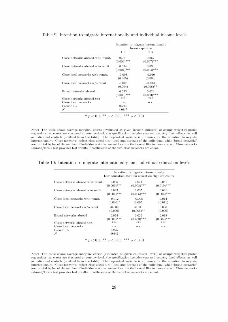
Table 9: Intention to migrate internationally and individual income levels

Intention to migrate internationallyIncome quintile

1–3 4–5

Close networks abroad with remit. 0.071 0.062(0.009)*** (0.007)***

Close networks abroad w/o remit. 0.034 0.033(0.004)*** (0.004)***

Close local networks with remit. -0.008 -0.010(0.005) (0.006)

Close local networks w/o remit. -0.006 -0.014(0.004) (0.006)**

Broad networks abroad 0.023 0.024(0.003)*** (0.003)***

Close networks abroad test *** ***Close local networks n.s. n.s.Pseudo R2 0.224N 48647

* p < 0.1; ** p < 0.05; *** p < 0.01

Note: The table shows average marginal effects (evaluated at given income quintiles) of sample-weighted probitregressions, st. errors are clustered at country-level, the specification includes year and country fixed effects, as wellas individual controls (omitted from the table). The dependent variable is a dummy for the intention to migrateinternationally. ‘Close networks’ reflect close social ties (local and abroad) of the individual, while ‘broad networks’are proxied by log of the number of individuals at the current location that would like to move abroad. Close networks(abroad/local) test provides test results if coefficients of the two close networks are equal.

Table 10: Intention to migrate internationally and individual education levels

Intention to migrate internationallyLow education Medium education High education

Close networks abroad with remit. 0.055 0.074 0.081(0.009)*** (0.008)*** (0.019)***

Close networks abroad w/o remit. 0.033 0.035 0.031(0.004)*** (0.005)*** (0.006)***

Close local networks with remit. -0.012 -0.008 0.014(0.006)* (0.005) (0.011)

Close local networks w/o remit. -0.009 -0.011 0.006(0.006) (0.005)** (0.009)

Broad networks abroad 0.024 0.026 0.018(0.003)*** (0.003)*** (0.004)***

Close networks abroad test *** *** ***Close local networks n.s. n.s. n.s.Pseudo R2 0.225N 48647

* p < 0.1; ** p < 0.05; *** p < 0.01

Note: The table shows average marginal effects (evaluated at given education levels) of sample-weighted probitregressions, st. errors are clustered at country-level, the specification includes year and country fixed effects, as wellas individual controls (omitted from the table). The dependent variable is a dummy for the intention to migrateinternationally. ‘Close networks’ reflect close social ties (local and abroad) of the individual, while ‘broad networks’are proxied by log of the number of individuals at the current location that would like to move abroad. Close networks(abroad/local) test provides test results if coefficients of the two close networks are equal.

28

are 7.1% more likely to intend to migrate internationally if they have close socialnetworks from which they receive remittances, while those with close social networkswithout remittances are only 3.4% more likely to plan to migrate internationally. Forthose with higher incomes, the impact of close social networks abroad is quite similar,being 6.2% with and 3.3% without remittances. However, interaction with educationhighlights some differences between the different groups. Close social networks abroadwith remittances matter significantly more than close social networks without remit-tances as the individuals become more educated. Social networks with remittancesincrease the likelihood of international migration intentions, with magnitude of thiseffect increasing with education level. The coefficient on close social network withremittances is about 2.6 times bigger than for close social networks without remit-tances for the highly educated individuals, about 1.7 times bigger for low-educatedand about 2.1 times bigger for medium-educated individuals.

One possible explanation for these results is that remittances coming from closesocial networks abroad not only provide direct financial assistance, but also have asignalling function for those who intend to migrate internationally. Possibly, higher-educated individuals are more likely to be able to take up relatively higher-payingjobs, or expect to be able to do so. To these individuals, close social networks abroadwith remittances send a signal that those sending the remittances are relatively richeror work in higher-paying jobs and are more likely to be able to eventually help find-ing/obtaining better-paying jobs (for further references examining the link betweensocial networks and job search see Munshi 2003; Comola and Mendola 2015). Onthe other hand, those with only primary school level of education are unlikely tolook for this kind of signal as they are unlikely to expect to be able to take up ahigher-paying job, which typically would require higher skill levels. Networks sendingremittances are relatively more important for all groups than networks without re-mittances, which indicates that these networks play a role in providing financial helpto cover some costs of migrating. For high education group, remittances could alsosend a signal of potential help in finding better-paying jobs.23

Close local networks with and without remittances on the other hand seem to playslightly different roles for lower- and higher-income individuals, while being less im-portant than networks abroad in general. For lower-income individuals, both typesof close local networks have a negative sign, but the coefficients are insignificant.Furthermore, for higher-income individuals, only those local networks have a signif-icant impact which do not involve financial assistance, decreasing the probability ofmigration intention by 1.4% (with only 5% significance).

The impact of close local social networks also varies with education levels. Wefind that having stronger social ties at home reduces the likelihood of the intentionto migrate for low- and medium-educated individuals, but has no impact on thosewith high education level. Higher-educated individuals seem to be unconstrained bylocal social networks. In addition, close local networks without remittances matter

23It should be noted however, that although our social network variable abroad always proxiesclose ties (family or close friends), it could be, that those networks with financial assistance fostermore migration intention not because of financial facilitation but because they represent even closerties.

29

more across all income and education groups. These findings indicate that closelocal networks influence international migration only marginally. In addition, peopleare less likely to be influenced if they have a local network from which they receivefinancial assistance. This could be because in networks from which they do not receiveremittances they are more likely to have others relying on them, making migrationmore difficult. Further micro-level data on the composition and strength of socialnetworks is needed to examine these alternative hypotheses.

6.5 Reverse causality

There is a possibility that those who plan to migrate first decide that they want tomigrate and then they request that close friends and family members abroad sendremittances to cover expenses related to emigrating. If this is the case, we have aproblem of reverse causality and we might be misinterpreting some of the resultsabove. In order to check if this type of reverse causality is driving the results, werestrict the sample to those individuals who themselves send remittances. Presum-ably, if an individual sends remittances she is not in need of receiving remittancesin order to cover the costs of migrating. Thus migration intentions are not likely todrive received remittances, so for this sub-sample reverse causality is less likely. Thequestion from the survey related to the individual sending remittances was not askedin all years and restricts us to year 2012.

The main results on our social network variables hold with this sample restriction,see Section 6 of the Online Appendix.24 As before, there is no important difference be-tween the relative importance of close networks abroad with and without remittancesbetween high- and low-income individuals (except for the low-income individuals withintention to migrate locally). In addition, as before, when looking at individuals withdifferent education level, close networks abroad with remittances are relatively moreimportant than without remittances in increasing the probability of migration inten-tion for highly educated individuals than for those with lower levels of educations.

7 Conclusions

Using a unique survey dataset, we explored how the intention to migrate internation-ally and domestically is influenced by different types of social networks, individualperception of amenities at country and local levels, and other individual character-istics. We distinguished between close social networks abroad and at home, withfurther distinction depending on whether these networks provide remittances or not.We also controlled for broad networks (same-country residents with intention to mi-grate either internationally or locally). We investigated the impact of these differentnetworks on individuals with different income and education levels.

This analysis provides several interesting results. First, close and broad networksare shown to explain the largest share of variation in the probability of international

24These tables are based on specifications that include broad networks, we also tried country fixedeffects specifications and the results are very similar.

30

migration intention. The robustness checks provide support to the causal directionfrom social networks to the intention to migrate. Close and broad social networksabroad combined are much more important than work-related factors, income orwealth. On the other hand, close networks at the current location reduce the like-lihood of the intention to migrate, albeit their importance is much lower. Second,when interacting networks with individual’s income and education level, we find thatwhile close networks abroad with remittances are more important than those withoutremittances for all groups, they are relatively more important for highly educatedindividuals. These results could indicate that close networks abroad which providefinancial assistance possibly play a role in covering parts of migration costs, but alsofor the highly educated individuals such networks could send a signal about potentialassistance in finding better paying jobs. Third, close local networks do not influencesignificantly migration intentions of highly educated individuals. A possible interpre-tation is that the networks which do not provide remittances are in turn dependenton the individual, hence reducing their intention to out-migrate.

Further micro-level data on the composition and strength of social networks isneeded to examine these alternative hypotheses about the mechanisms through whichdifferent social networks influence the intention to migrate. A limitation of our em-pirical analysis is that we do not look at bilateral migration intentions, as we donot have information in which country the close network of the individual is located.Hence, using better micro-level data could provide further insights on the role of closenetworks.

References

Banerjee, B. (1983). “Social networks in the migration process: empirical evidence onchain migration in India”. The Journal of Developing Areas 17.2, pp. 185–196.

Beine, M., F. Docquier, and C. Ozden (2011). “Diasporas”. Journal of DevelopmentEconomics 95.1. Symposium on Globalization and Brain Drain, pp. 30–41.

Beine, M. and S. Salomone (2012). “Network effects in international migration: ed-ucation versus gender”. The Scandinavian Journal of Economics 115.2, pp. 354–380.

Bell, M., E. Charles-Edwards, D. Kupiszewska, M. Kupiszewski, J. Stillwell, and Y.Zhu (2015). “Internal migration data around the world: Assessing contemporarypractice”. Population, Space and Place 21.1, pp. 1–17.

Bertoli, S. and I. Ruyssen (2016). “Networks and migrants′ intended destination”.IZA discussion paper 10213.

Boyd, M. (1989). “Family and Personal Networks in International Migration: RecentDevelopments and New Agendas”. International Migration Review 23.3, pp. 638–670.

Brucker, H., S. Capuano, and A. Marfouk (2013). “Education, gender and interna-tional migration: insights from a panel-dataset 1980-2010”. mimeo.

31

Chavez Juarez, F. W. (2015). “shapley2: a Stata program to compute the Shapleyvalues”. Online software.

Chen, Y. and S. S. Rosenthal (2008). “Local amenities and life-cycle migration: dopeople move for jobs or fun?” Journal of Urban Economics 64.3, pp. 519–537.

Chuang, Y. and L. Schechter (2015). “Social Networks in Developing Countries”.Annual Review of Resource Economics 7.1. eprint: http://dx.doi.org/10.1146/annurev-resource-100814-125123.

Comola, M. and M. Mendola (2015). “Formation of Migrant Networks”. The Scandi-navian Journal of Economics 117.2, pp. 592–618.

Creighton, M. J. (2013). “The role of aspirations in domestic and international mi-gration”. The Social Science Journal 50.1, pp. 79–88.

De Simone, G. and M. Manchin (2012). “Outward migration and inward FDI: factormobility between Eastern and Western Europe”. Review of International Eco-nomics 20.3, pp. 600–615.

Docquier, F., A. Marfouk, S. Salomone, and K. Sekkat (2012). “Are skilled womenmore migratory than skilled men?” World Development 40.2, pp. 251–265.

Docquier, F., G. Peri, and I. Ruyssen (2014). “The Cross-country Determinants ofPotential and Actual Migration”. International Migration Review 48.S1, S37–S99.

Docquier, F. and H. Rapoport (2012). “Globalization, Brain Drain, and Develop-ment”. Journal of Economic Literature 50.3, pp. 681–730.

Docquier, F., A. Tansel, and R. Turati (2017). “Do Emigrants Self-Select Along Cul-tural Traits?: Evidence from the MENA Countries”. IRES Discussion Paper 2017-24.

Donato, K. M., J. Durand, and D. S. Massey (1992). “Changing Conditions in theUS Labor Market: Effects of the Immigration Reform and Control Act of 1986”.Population Research and Policy Review 11.2, pp. 93–115.

Dustmann, C. and A. Okatenko (2014). “Out-migration, wealth constraints, and thequality of local amenities”. Journal of Development Economics 110, pp. 52–63.

Esipova, N., J. Ray, and A. Pugliese (2011). “Gallup World Poll: the many faces ofglobal migration”. IOM Migration Research Series, No. 43.

Flores-Yeffal, N. Y. and M. Aysa-Lastra (2011). “Place of Origin, Types of Ties, andSupport Networks in Mexico-US Migration”. Rural Sociology 4.76, pp. 481–510.

Friebel, G., M. Manchin, M. Mendola, and G. Prarolo (2017). “Human Smugglingand Intentions to Migrate: Global Evidence from a Supply Shock along Africa-to-Europe Migration Routes”.

Gallup (2012). “Worldwide research methodology and codebook”.

Garip, F. and A. L. Asad (2016). “Network Effects in Mexico–US Migration: Disentan-gling the Underlying Social Mechanisms”. American Behavioral Scientist 60.10,pp. 1168–1193.

Giulietti, C., J. Wahba, and Y. Zenou (2018). “Strong versus weak ties in migration”.European Economic Review. forthcoming.

Hatton, T. J. and J. G. Williamson (2005). “What fundamentals drive world migra-tion?” Poverty, international migration and asylum. Springer, pp. 15–38.

32

Javorcik, B. S., C. Ozden, M. Spatareanu, and C. Neagu (2011). “Migrant networksand foreign direct investment”. Journal of Development Economics 94.2, pp. 231–241.

Kandel, W. and D. S. Massey (2002). “The culture of Mexican migration: A theoret-ical and empirical analysis”. Social forces 80.3, pp. 981–1004.

Kerr, W. R. (2008). “Ethnic scientific communities and international technology dif-fusion”. The Review of Economics and Statistics 90.3, pp. 518–537.

King, R. and R. Skeldon (2010). ““Mind the Gap!” Integrating Approaches to Internaland International Migration”. Journal of Ethnic and Migration Studies 36.10,pp. 1619–1646.

Knapp, T. A. and P. E. Gravest (1989). “On the role of amenities in models ofmigration and regional development”. Journal of Regional Science 29.1, pp. 71–87.

Liu, M.-M. (2013). “Migrant networks and international migration: Testing weakties”. Demography 50.4, pp. 1243–1277.

Manski, C. F. (1993). “Identification of endogenous social effects: The reflection prob-lem”. The review of economic studies 60.3, pp. 531–542.

Massey, D. S., J. Arango, G. Hugo, A. Kouaouci, A. Pellegrino, and T. J. Edward(1993). “Theories of international migration: review and appraisal. Population andDevelopment”. Population and Development Review 3.19, pp. 431–466.

Mayda, A. M. (2010). “International migration: a panel data analysis of the determi-nants of bilateral flows”. Journal of Population Economics 23.4, pp. 1249–1274.

McKenzie, D. and H. Rapoport (2007). “Network effects and the dynamics of migra-tion and inequality: theory and evidence from Mexico”. Journal of DevelopmentEconomics 84.1, pp. 1–24.

McKenzie, D. and H. Rapoport (2010). “Self-Selection Patterns in Mexico-U.S. Mi-gration: The Role of Migration Networks”. Review of Economics and Statistics92.4, pp. 811–821.

Mendola, M. (2008). “Migration and technological change in rural households: com-plements or substitutes?” Journal of Development Economics 85.1, pp. 150–175.

Munshi, K. (2003). “Networks in the Modern Economy: Mexican Migrants in the U.S. Labor Market”. The Quarterly Journal of Economics 118.2, pp. 549–599.

Munshi, K. (2014a). “Community networks and migration”. The Oxford handbook ofthe economics of networks. Oxford University Press.

Munshi, K. (2014b). “Community Networks and the Process of Development”. Jour-nal of Economic Perspectives 28.4, pp. 49–76.

Munshi, K. and M. Rosenzweig (2016). “Networks and Misallocation: Insurance, Mi-gration, and the Rural-Urban Wage Gap”. American Economic Review 106.1,pp. 46–98.

Niedomysl, T. and H. K. Hansen (2010). “What matters more for the decision tomove: jobs versus amenities”. Environment and planning. A 42.7, pp. 1636–1649.

Ortega, F. and G. Peri (2009). “The causes and effects of international migrations:Evidence from OECD countries 1980-2005”. 14833. NBER working paper 14833.

33

Rubalcava, L. N., G. M. Teruel, D. Thomas, and N. Goldman (2008). “The healthymigrant effect: new findings from the Mexican Family Life Survey”. Journal In-formation 98.1.

Ruyssen, I. and S. Salomone (2018). “Female migration: a way out of discrimination?”Journal of Development Economics 130, pp. 224–241.

Scott, A. J. (2010). “Jobs or amenities? Destination choices of migrant engineers inthe USA”. Papers in Regional Science 89.1, pp. 43–63.

Shorrocks, A. F. (1982). “Inequality decomposition by factor components”. Econo-metrica 50.1, pp. 193–211.

Sjaastad, L. A. (1962). “Costs And Returns of Human Migration”. Journal of PoliticalEconomy 70.5, pp. 80–93.

Takenaka, A. and K. A. Pren (2010). “Determinants of emigration: comparing mi-grants’ selectivity from Peru and Mexico”. The ANNALS of the American Academyof Political and Social Science 630.1, pp. 178–193.

Toma, S. and S. Vause (2014). “Gender differences in the role of migrant networks:Comparing Congolese and Senegalese migration flows”. International MigrationReview 48.4, pp. 972–997.

UNDP (2009). Human development report. Overcoming barriers: human mobility anddevelopment.

van Dalen, H. P. and K. Henkens (2013). “Explaining emigration intentions and be-haviour in the Netherlands, 2005-2010”. Population Studies 67.2, pp. 225–241.

34

Online appendix to accompany the paper:Social networks and the intention to migrate

Miriam Manchin∗ Sultan Orazbayev†

March 17, 2018

All calculations are our own, unless specified otherwise. Maps were drawnusing ‘spmap’ command for Stata: M. Pisati (2017). “SPMAP: Stata moduleto visualize spatial data”.

Contents

1 Distinguishing between intentions to migrate locally and in-ternationally 2

2 Construction of principal component-based indexes with PCA 52.1 Local amenities and local security . . . . . . . . . . . . . . . . 62.2 Contentment with the country and country-level corruption . . 72.3 Work . . . . . . . . . . . . . . . . . . . . . . . . . . . . . . . . 82.4 Wealth and standard of living . . . . . . . . . . . . . . . . . . 92.5 Close local networks . . . . . . . . . . . . . . . . . . . . . . . 9

3 Sample coverage 10

4 Additional descriptives by region 13

5 Supplementary tables for specifications reported in the mainpaper 13

6 Full tables for specifications with sample restricted to thosethat send remittances 16

7 Marginal effects with family abroad 19

8 Variation across regions and country income groups: localmigration intentions 21

9 Results with individual income and education 23

∗University College London, Gower Street, WC1E 6BT, UK; e-mail:m.manchin@ucl.ac.uk; phone/fax: +44(0)2076798765.†Center for International Development, Harvard University, Cambridge, MA 02138,

USA; contact@econpoint.com; phone/fax: +1 6174951100.

1

10 Results with actual migration data for broad networks abroad 25

11 Results with a stronger intention (including preparation) 28

12 Sample restricted to country natives only 29

13 Results with lagged peers and country-year fixed effects 32

14 Results with country-year random effects 32

1 Distinguishing between intentions to mi-

grate locally and internationally

Gallup’s World Poll survey contains several questions that can help distin-guish between intention to migrate locally and internationally (and possiblydistinguishing temporary and permanent moves, as well as comparing weakwith strong intentions). The relevant questions are:

• WP85: “In the next 12 months, are you likely or unlikely to move awayfrom the city or area where you live?”

• WP1325: “Ideally, if you had the opportunity, would you like to movePERMANENTLY to another country, or would you prefer to continueliving in this country?”

• WP10252: “Are you planning to move permanently to another countryin the next 12 months, or not?” (WP10252 is asked only for individualsthat responded “Yes” to WP1325.)

• WP9455: “Have you done any preparation for this move? (For example,applied for residency or visa, purchased the ticket, etc.)” (WP9455 isasked only for individuals that responded “Yes” to WP10252.)

• WP9498: “Ideally, if you had the opportunity, would you like to go toanother country for temporary work, or not?”

The answer to WP85 can help identify individuals that are likely to out-migrate — locally or internationally. Arguably, WP85 elicits firmer inten-tions than those elicited by questions WP1325 and WP9498 (“. . . are youlikely to move. . . ” vs. “ideally, if you had the opportunity, would you like tomove. . . ”). The closest phrasing is in question WP10252: similar time peri-ods (next 12 months), relatively firm intention (there is no reference to ideal

2

conditions or opportunities); and in question WP9455: similar time periodand firm intention (steps already taken).

A rigorous interpretation of WP85 and WP10252/9455 would requiremany further clarifications to make them congruent. Firstly, WP85 doesnot contain indication of the length of the move (temporary vs. perma-nent), while WP10252 is specifically applicable to permanent migration. Thismeans that for further comparison we need to assume that WP85 is inter-preted for permanent moves. Secondly, it is possible that an individual willmove locally before permanently migrating abroad. This means that separa-tion between local and international migration will be based only on intendedfinal destination in 12 months’ time. Thirdly, in terms of firmness of inten-tions WP85 appears to be between WP10252, which is a bit weaker thanWP85, and WP9455, which is a bit stronger than WP85. Since WP9455 isasked only given positive response to WP10252, the sample size will be largerif WP10252 is used for comparison with WP85. The procedure below can bemodified to use WP9455 instead, if needed. Fourthly, there could be differentinterpretation of WP1325 by natives and current migrants. Current migrantsmight not think of returning home as a permanent move to another country.This issue will be ignored in the procedure below, but can be addressed tosome extent by filtering out current migrants from the sample.

Assuming that individuals interpret questions WP85 and WP10252 ina similar way, it is possible to use these questions to distinguish betweenthose that intend to move locally and internationally. The intended finaldestination in 12 months’ time can be: current location, domestic location(local migration), or foreign location (international migration).

Table 1 summarizes possible combinations and separates individuals intothree categories, depending on their intention to stay, migrate locally orinternationally. The number of observations in each category is presented inTable 1 in the main paper.

3

Table 1: Identifying intentions to migrate locally and internationally - moti-vation

Are youlikely tomoveA?

Would you like tomove abroadB?

Are youplanningto move

abroadC?

Imputedstatus

Motivation

Likely tomove

Like to continueliving in this

country

Thequestion isnot asked.

Intention tomigratelocally

Likely to move locally, becausethere is no expression of a desire tomove abroad.

Like to move toanother country

No

Dreamer(movinglocally)

Likely to move locally, since themove abroad will be taken only un-der ideal conditions.

Yes, willmove innext 12months

Intention tomigrate inter-

nationallyLikely to move internationally, sinceindicated move (WP85) and tooksteps for moving to a foreign loca-tion.

Not likelyto move

Like to continueliving in this

country

Thequestion isnot asked.

Intention tostay

Not likely to move.

Like to move toanother country

No Dreamer Would like to move away, but no in-tention to do so in the near future.

Yes, willmove inthe next

12 months

Contradictoryresponse

The response to WP85 contradictsanswer to WP10252. Can treatthese responses as either stayers orinternational migrants, or alterna-tively can discard these observations(the last option is used for this pa-per).

Notes:A Full question: “In the next 12 months, are you likely or unlikely to move away from thecity or area where you live?”B Full question: “Ideally, if you had the opportunity, would you like to move PERMA-NENTLY to another country, or would you prefer to continue living in this country?”C Full question: “Are you planning to move permanently to another country in the next12 months, or not? (asked only of those who would like to move to another country)”

4

IndividualcomparesE(u) with

0 (notmigrating)

Weak inten-tion to migrate

Decide tostay at

the origin

Strongintention

to migrate

Decide tostay at

the origin

E(u) > 0

E(u) ≤ 0

ωo ≥ c

ωo < c

Figure 1: Decision tree for the individual: weak vs. strong intention

2 Construction of principal component-based

indexes with PCA

The survey contains many questions which are relevant for our analysis andare related to similar issues. Including just one variable for a given topiccould lead to loss of information, including all variables will result in mul-ticollinearity. Instead of limiting the analysis to one of these questions, weretain as much information as possible in the underlying data and use prin-cipal component analysis (PCA) to produce a set of indexes to use in ourmain specifications.

PCA is a statistical technique that has been widely applied in fields suchas face recognition and image compression, and is a common method ofreducing data dimensionality. Ideally, principal component analysis identifiespatterns in the data and based on these patterns it reduces the number ofdimensions of the data without a large loss of information. It reduces thedata to a few principal components by using the variance structure of thematrix of data through linear combination of the variables. Given that mostof the variables used for constructing the indexes are not continuous, we usepolychoric PCA (Kolenikov and Angeles 2004).1

Our main objective in using PCA is to reduce the dimensionality of thedata. The original survey questions were grouped in categories by Gallup.Following these categories, and limiting the data to questions which were

1As a robustness check we also run standard principal component analysis and theresults are very similar.

5

available for most years and countries, we group questions into the followingcategories: ‘local amenities and local security’, ‘country contentment andcorruption’, ‘work’, ‘wealth and standard of living’, ‘close local networks’.For some categories only two or three questions were available for sufficientcoverage. In these cases we only retain the first component. When morethan three underlying variables were used, we retain the first two componentsof the principal component analysis. This is supported by the eigenvaluesbeing greater or close to 1, which is a widely used cut-off rule (see Hatcher andO’Rourke 2014).2 We retain the first component for the ‘work’ and ‘close localnetworks’, and the first two components for ‘wealth and standard of living’,‘local amenities and secuirty’, and ‘country contentment and corruption’. Foreach category the resulting components together reflect between roughly 60and 67% of variation of the underlying sample (indicated in the table by thecumulative proportion explained). All indexes were scaled to range from 0to 1. Table 2 summarises the constructed indexes.

Table 2: Overview of the constructed indexes

Proportion Cumulative

Category Component Eigenvalue explained proportion

Local amenities and security Local amenities 3.76 0.47 0.47Local amenities and security Local security 0.99 0.12 0.59Country contentment and corruption Contentment with the country 4.11 0.51 0.51Country contentment and corruption Corruption 1.31 0.16 0.67Work Work 1.90 0.63 0.63Wealth and standard of living Wealth 3.96 0.44 0.44Wealth and standard of living Standard of living 1.39 0.15 0.59Close local networks Close local networks 1.21 0.60 0.60

2.1 Local amenities and local security

Table 3: List of questions used

2Every variable contributes one unit of variance to the total variance in the dataset,so the component with eigenvalue greater than 1 represents greater variance than wascontributed by a single variable.

6

Label Full question

Satisfaction with the city/area Are you satisfied or dissatisfied with the city or area where you live?Satisfaction with the public transportation system In the city or area where you live, are you satisfied or dissatisfied with

the public transportation systems?Satisfaction with the roads/highways In the city or area where you live, are you satisfied or dissatisfied with

the roads and highways?Satisfaction with the schools/education system In the city or area where you live, are you satisfied or dissatisfied with

the educational system or the schools?Satisfaction with the availability of healthcare In the city or area where you live, are you satisfied or dissatisfied with

the availability of quality healthcare?Satisfaction with the availability of housing In the city or area where you live, are you satisfied or dissatisfied with

the availability of good, affordable housing?Satisfaction with the beauty or physical setting In the city or area where you live, are you satisfied or dissatisfied with

the beauty or physical setting?Personal safety at night Do you feel safe walking alone at night in the city or area where you

live?

Table 4: The first three components

Component 1 Component 2 Component 3Proportion explained 0.470 0.124 0.101Proportion explained (cumulative) 0.470 0.594 0.695Eigenvalue 3.761 0.991 0.806

Table 5: The first three eigenvectors

Variable/response Component 1 Component 2 Component 3

Satisfaction with the city/area 0.35 0.24 0.07Satisfaction with the public transportation system 0.37 -0.43 0.29Satisfaction with the roads/highways 0.38 -0.39 0.27Satisfaction with the schools/education system 0.39 -0.17 0.00Satisfaction with the availability of healthcare 0.40 -0.06 -0.18Satisfaction with the availability of housing 0.35 0.21 -0.50Satisfaction with the beauty or physical setting 0.35 0.30 -0.38Personal safety at night 0.21 0.66 0.64

Based on these results, the first principal component is labelled as ‘localamenities’ and the second component as ‘local security’.

2.2 Contentment with the country and country-levelcorruption

Table 6: List of questions used.

7

Label Full question

Confidence in the military In this country, do you have confidence in each of the following, or not?How about the military?

Confidence in the judicial system/courts In this country, do you have confidence in each of the following, or not?How about judicial system and courts?

Confidence in the national government In this country, do you have confidence in each of the following, or not?How about national government?

Confidence in the fair elections In this country, do you have confidence in each of the following, or not?How about honesty of elections?

Spread of corruption in business Is corruption widespread within businesses located in this country, ornot?

Spread of corruption in government Is corruption widespread throughout the government in this country, ornot?

Approval of country leadership’s job performance Do you approve or disapprove of the job performance of the leadershipof this country?

Change in the country’s economic conditions Right now, do you think that economic conditions in this country, as awhole, are getting better or getting worse?

Table 7: The first three components

Component 1 Component 2 Component 3Proportion explained 0.514 0.164 0.116Proportion explained (cumulative) 0.514 0.678 0.794Eigenvalue 4.113 1.309 0.931

Table 8: The first three eigenvectors

Variable/response Component 1 Component 2 Component 3

Confidence in the military 0.32 -0.32 -0.43Confidence in the judicial system/courts 0.38 -0.22 -0.35Confidence in the national government 0.43 -0.21 0.06Confidence in the fair elections 0.37 -0.03 -0.19Spread of corruption in business 0.28 0.66 -0.09Spread of corruption in government 0.34 0.57 -0.02Approval of country leadership’s job performance 0.38 -0.16 0.39Change in the country’s economic conditions 0.29 -0.11 0.70

Based on these results, the first principal component is labelled as ‘content-ment with the country’ and the second component as ‘corruption’.

2.3 Work

Table 9: List of questions usedLabel Full question

Job opportunities In the city or area where you live, are you satisfied or dissatisfied withthe availability of good job opportunities?

Job satisfaction Are you satisfied or dissatisfied with your job or the work you do? (withmodifications - see text)

Employment Employment Status (with modifications - see text)

Table 10: The first three components

8

Component 1 Component 2 Component 3Proportion explained 0.633 0.291 0.076Proportion explained (cumulative) 0.633 0.924 1.000Eigenvalue 1.899 0.874 0.227

Table 11: The first three eigenvectors

Variable/response Component 1 Component 2 Component 3

Job opportunities 0.38 0.91 0.19Job satisfaction 0.67 -0.13 -0.73Employment 0.63 -0.40 0.66

Based on these results, the first principal component is labelled as ‘work’.

2.4 Wealth and standard of living

Table 12: List of questions usedLabel Full question

Income quintile Household income within country quintiles.Perception of present income Which one of these phrases comes closest to your own feelings about

your household income these days?Current standard of living Are you satisfied or dissatisfied with your standard of living, all the

things you can buy and do?Changes in standard of living Right now, do you feel your standard of living is getting better or get-

ting worse?Mobile phone at home Does your home have a cellular phone?Television at home Does your home have a televisionInternet access at home Does your home have access to the Internet?Money for food Have there been times in the past 12 months when you did not have

enough money to buy food that you or your family needed?Money for shelter Have there been times in the past 12 months when you did not have

enough money to provide adequate shelter or housing for you and yourfamily?

Table 13: The first three components

Component 1 Component 2 Component 3Proportion explained 0.440 0.154 0.117Proportion explained (cumulative) 0.440 0.594 0.711Eigenvalue 3.961 1.387 1.050

Based on these results, the first principal component is labelled as ‘wealth’and the second component as ‘standard of living’.

2.5 Close local networks

Table 15: List of questions usedLabel Full question

Opportunities to make friends In the city or area where you live, are you satisfied or dissatisfied withthe opportunities to meet people and make friends?

Help available If you were in trouble, do you have relatives or friends you can counton to help you whenever you need them, or not?

9

Table 14: The first three eigenvectors

Variable/response Component 1 Component 2 Component 3

Income quintile 0.25 0.02 0.40Perception of present income 0.36 0.20 0.17Current standard of living 0.35 0.40 0.12Changes in standard of living 0.22 0.57 0.29Mobile phone at home 0.34 -0.41 0.22Television at home 0.37 -0.38 0.04Internet access at home 0.38 -0.37 0.05Money for food 0.39 0.10 -0.45Money for shelter 0.30 0.12 -0.67

Table 16: The first two components

Component 1 Component 2Proportion explained 0.603 0.397Proportion explained (cumulative) 0.603 1.000Eigenvalue 1.206 0.794

Table 17: The first two eigenvectors

Variable/response Component 1 Component 2

Opportunities to make friends 0.71 0.71Help available (local and abroad) 0.71 -0.71

Based on these results, the first principal component is labelled as ‘close localnetworks’.

3 Sample coverage

10

Table 18: List of countries and their sample size

P S P S P SAfghanistan 680 1453 Ghana 616 1322 Palestinian Territories 270 1746Albania 287 1501 Greece 515 2262 Panama 573 2101Algeria 0 1877 Guatemala 324 1376 Paraguay 760 2412Argentina 515 2192 Guinea 548 943 Peru 639 1890Armenia 338 1930 Haiti 150 479 Philippines 1304 3251Australia 418 876 Honduras 513 1899 Poland 282 1775Austria 210 1286 Hong Kong 241 776 Portugal 138 927Azerbaijan 202 660 Hungary 350 1636 Qatar 0 877Bahrain 0 749 India 4777 10416 Romania 229 1304Bangladesh 531 2311 Indonesia 743 2483 Russia 1009 5007Belarus 103 1591 Iraq 177 1256 Rwanda 0 1778Belgium 76 318 Ireland 327 964 Saudi Arabia 0 1594Benin 596 930 Israel 272 1203 Senegal 930 2320Bolivia 689 1589 Italy 111 596 Serbia 205 2000Bosnia and Herzegovina 248 1998 Japan 237 1217 Sierra Leone 478 851Botswana 453 860 Jordan 0 1625 Singapore 0 765Brazil 693 2415 Kazakhstan 277 1577 Slovakia 391 1415Bulgaria 252 2019 Kenya 1428 1869 Slovenia 272 1140Burkina Faso 1089 1853 Kosovo 249 1534 Somalia 1656 2940Burundi 0 768 Kuwait 0 808 South Africa 1233 1918Cambodia 912 1863 Kyrgyzstan 585 2287 South Korea 215 1144Cameroon 585 2062 Latvia 217 968 Spain 320 1437Canada 16 1427 Lebanon 0 1707 Sri Lanka 225 1407Central African Republic 449 863 Liberia 480 820 Sudan 0 2661Chad 1242 2603 Lithuania 402 1479 Suriname 125 335Chile 602 2219 Luxembourg 252 742 Sweden 365 1266China 0 5360 Macedonia 131 1973 Switzerland 0 554Colombia 764 2238 Madagascar 657 959 Syria 0 1035Comoros 1404 2789 Malawi 648 1532 Tajikistan 216 2225Congo (Kinshasa) 382 1303 Malaysia 550 2225 Tanzania 1415 2569Costa Rica 587 1446 Mali 609 1589 Thailand 1465 3402Croatia 153 1872 Malta 68 416 Tunisia 288 1627Cyprus 178 952 Mauritania 1385 2640 Turkey 771 2905Czech Republic 521 2025 Mexico 369 1279 Uganda 1341 2332Denmark 335 1461 Moldova 358 1679 Ukraine 476 1674Djibouti 284 871 Mongolia 427 1569 United Arab Emirates 0 1524Dominican Republic 761 2012 Montenegro 231 1771 United Kingdom 170 1083Ecuador 353 1470 Myanmar 0 848 United States 38 1453Egypt 0 954 Nepal 478 1442 Uruguay 430 2053El Salvador 490 1849 Netherlands 257 670 Uzbekistan 0 2447Estonia 175 744 New Zealand 256 593 Venezuela 528 2107Finland 357 843 Nicaragua 560 2018 Vietnam 0 1282France 165 1321 Niger 1172 2732 Yemen 0 1743Georgia 267 1437 Nigeria 1033 2750 Zambia 527 871Germany 289 1253 Pakistan 610 1471 Zimbabwe 1007 1822

Note: numbers in column “P” represent sample size using principal component-based indexes, numbers

in columns “S” represent sample size using single questions.

11

Figure 2: Geographic coverage of the sample used for estimation with theconstructed indexes

Note: Countries included in the estimations are shaded in dark colour, other countries arenot included. See the Appendix in the paper for actual observation counts.

Figure 3: Geographic coverage of the sample with the single variables speci-fication

Note: Countries included in the estimations are shaded in dark colour, other countries arenot included. See the Appendix in the paper for actual observation counts.

12

4 Additional descriptives by region

Table 19: Average values for network variables

Close networks: Broad networks:abroad local abroad local

European Union 0.404 0.87 0.01 0.08Balkans 0.347 0.74 0.02 0.05Europe-other 0.91 0.09Commonwealth of Independent States 0.281 0.76 0.01 0.06Australia-New Zealand 0.622 0.93 0.02 0.14Southeast Asia 0.205 0.84 0.00 0.08South Asia 0.144 0.67 0.00 0.12East Asia 0.186 0.81 0.00 0.10Latin America and the Caribbean 0.415 0.83 0.02 0.16Northern America 0.318 0.91 0.00 0.16Middle East and North Africa 0.327 0.75 0.01 0.17Sub-Saharan Africa 0.324 0.73 0.04 0.20Minimum value 0.144 0.67 0.00 0.05Maximum value 0.622 0.93 0.04 0.20

Note: Close networks measure whether the respondent has friends/family locally or abroad that can

provide support. Broad networks measure the share of individuals in the same country as the respondent

that expressed intention to migrate. Values for region “Europe-other” are missing due to lack of responses

to the relevant questions in the sample for that region.

Table 20: Average values for selected variables

Local Contentment with Standard ofamenities security the country Corruption Work Wealth living

European Union 0.722 0.57 0.48 0.38 0.71 0.73 0.40Balkans 0.634 0.59 0.30 0.31 0.58 0.65 0.38Europe-other 0.818 0.60 0.69 0.46 0.84 0.83 0.48Commonwealth of Independent States 0.635 0.57 0.44 0.29 0.66 0.60 0.46Australia-New Zealand 0.750 0.57 0.67 0.51 0.78 0.81 0.47Southeast Asia 0.788 0.54 0.59 0.22 0.81 0.63 0.53South Asia 0.630 0.54 0.53 0.22 0.69 0.55 0.58East Asia 0.698 0.55 0.41 0.37 0.73 0.71 0.49Latin America and the Caribbean 0.648 0.51 0.40 0.37 0.69 0.62 0.52Northern America 0.757 0.61 0.58 0.40 0.68 0.78 0.47Middle East and North Africa 0.591 0.54 0.46 0.29 0.66 0.66 0.45Sub-Saharan Africa 0.484 0.58 0.47 0.30 0.54 0.44 0.56Minimum value 0.484 0.51 0.30 0.22 0.54 0.44 0.38Maximum value 0.818 0.61 0.69 0.51 0.84 0.83 0.58

Note: description of the variables is provided in the Appendix in the paper.

5 Supplementary tables for specifications re-

ported in the main paper

13

Table 21: Probit regression coefficients for specification in Table 4 in themain paper

Linear specification Non-linear specificationIntention to migrate

internationally locally internationally locally

Close local networks -0.146 -0.115 -0.147 -0.118(0.071)** (0.031)*** (0.071)** (0.031)***

Close networks abroad 0.603 0.147 0.602 0.147(0.041)*** (0.020)*** (0.041)*** (0.020)***

Broad networks abroad 0.447 0.448(0.050)*** (0.050)***

Broad local networks 0.463 0.458(0.083)*** (0.083)***

Local amenities -0.569 -0.470 -0.570 -0.473(0.078)*** (0.043)*** (0.078)*** (0.043)***

Local security -0.384 -0.408 -0.383 -0.407(0.090)*** (0.049)*** (0.090)*** (0.050)***

Contentment with the country -0.374 -0.057 -0.374 -0.056(0.089)*** (0.053) (0.088)*** (0.053)

Corruption -0.204 -0.045 -0.202 -0.044(0.113)* (0.079) (0.112)* (0.078)

Work -0.344 -0.265 -0.342 -0.261(0.065)*** (0.039)*** (0.065)*** (0.039)***

Wealth 0.200 0.070 0.497 0.662(0.110)* (0.088) (0.363) (0.218)***

Standard of living -0.465 -0.217 -0.210 -0.169(0.160)*** (0.071)*** (0.444) (0.342)

Wealth sq. -0.292 -0.558(0.348) (0.174)***

Standard of living sq. -0.250 -0.037(0.499) (0.344)

Married -0.209 -0.127 -0.209 -0.127(0.042)*** (0.023)*** (0.042)*** (0.023)***

Age -0.015 -0.014 -0.015 -0.014(0.002)*** (0.001)*** (0.002)*** (0.001)***

Education (medium) 0.103 0.094 0.102 0.093(0.055)* (0.024)*** (0.054)* (0.024)***

Education (high) 0.193 0.179 0.199 0.194(0.070)*** (0.029)*** (0.071)*** (0.029)***

Female -0.197 -0.075 -0.196 -0.075(0.041)*** (0.025)*** (0.041)*** (0.025)***

Large city 0.128 0.034 0.128 0.035(0.055)** (0.026) (0.055)** (0.025)

Healthy -0.153 -0.176 -0.153 -0.175(0.043)*** (0.041)*** (0.044)*** (0.041)***

# of children 0.019 -0.007 0.018 -0.007(0.009)** (0.005) (0.009)** (0.005)

Pseudo R2 0.22 0.10 0.22 0.10N 49,012 60,533 49,012 60,533

* p < 0.1; ** p < 0.05; *** p < 0.01

Note: The table shows coefficients of sample-weighted probit regressions, st. errors are clustered at country-level, all specifications include year and country fixed effects. The dependent variable is a dummy for theintention to migrate internationally (see text for details). The first specification includes ‘wealth’ and ‘stan-dard of living’ in a linear form, the second specification includes these variables and their squared values.‘Local amenities’ and ‘local security’ capture satisfaction at the city/local level, while ‘contentment withthe country’ and ‘corruption’ reflect individual’s satisfaction with the country-level institutions/amenities,‘work’ reflects satisfaction with the job, ‘close networks’ reflect social networks (local and abroad) of theindividual, while ‘broad networks’ are proxied by log of the number of other individuals at the currentlocation that would like to move locally and abroad. All of the indexes are principal components capturinginformation from the underlying variables.

14

Table 22: IV regressions with single questions (first stage)

Intention to migrateinternational international international local

Instruments for networksclose abroad broad abroad close abroad broad local

Region avg city satisfaction, 2-year lag -0.035 0.047 -0.040

(0.015)** (0.013)*** (0.015)***

Region avg rel income, 2-year lag 0.025 0.089 0.019

(0.006)*** (0.005)*** (0.005)***

Country avg perception of economy, 2-year lag 0.059 -0.789

(0.016)*** (0.025)***

Close local networks 0.026 -0.000 0.024 -0.011

(0.004)*** (0.003) (0.004)*** (0.001)***

Satisfaction with the city/area 0.017 -0.002 0.016 -0.002

(0.004)*** (0.003) (0.004)*** (0.001)**

Country economic condition (getting worse) 0.010 -0.003 0.009 0.005

(0.004)** (0.003) (0.004)** (0.001)***

Country economic condition (getting better) 0.046 0.009 0.045 0.011

(0.004)*** (0.003)*** (0.004)*** (0.001)***

Part-time employment -0.007 -0.002 -0.007 0.002

(0.007) (0.005) (0.007) (0.001)

Full-time employment -0.003 -0.002 -0.003 -0.002

(0.007) (0.005) (0.007) (0.001)

Log (rel.) income 0.064 -0.010 0.062 0.000

(0.002)*** (0.002)*** (0.002)*** (0.000)

Married -0.010 0.000 -0.009 0.000

(0.004)*** (0.003) (0.003)*** (0.001)

Age -0.000 0.000 -0.000 -0.000

(0.000) (0.000) (0.000)** (0.000)

Education (medium) 0.042 0.013 0.040 0.000

(0.004)*** (0.003)*** (0.004)*** (0.001)

Education (high) 0.096 0.006 0.098 0.003

(0.006)*** (0.004) (0.006)*** (0.001)**

Female 0.009 -0.001 0.008 -0.001

(0.003)*** (0.003) (0.003)** (0.001)

Large city 0.025 -0.017 0.026 0.004

(0.004)*** (0.003)*** (0.004)*** (0.001)***

Healthy -0.003 -0.001 -0.006 -0.007

(0.004) (0.003) (0.004) (0.001)***

# of children -0.003 0.001 -0.003 0.002

(0.001)*** (0.001) (0.001)** (0.000)***

Country avg city safety, 2-year lag 0.395

(0.016)***

Country avg city housing, 2-year lag 0.173

(0.016)***

Country avg city healthcare, 2-year lag 0.152

(0.020)***

N 96,623 96,623 104,888 139,762

* p < 0.1; ** p < 0.05; *** p < 0.01

Note: The table shows first-stage results for specifications in Table 8 in the main paper. The instrumentsused in the first and second columns — close networks abroad are instrumented with two-year lags ofregional-level satisfaction with the local city/area and relative income, while broad networks abroad areinstrumented with two-year lag of country-level perception of change in the country economy; the thirdcolumn uses the same instruments for close networks abroad and adds country-year fixed effects insteadof broad networks abroad. The dependent variable is an indicator for intention to move away from thecurrent location internationally. ‘Close networks abroad’ are measured by question ‘Do you have relativesor friends who are living in another country whom you can count on to help you when you need them?’,while ‘close local networks’ are measured by question ‘Are you satisfied with the opportunities to meetpeople and make friends?’. ‘Broad networks’ are proxied by the log of the total number of individuals atthe current location that intend to move abroad. ‘Local amenities’ are measured by ‘How satisfied areyou with your city?’.

15

6 Full tables for specifications with sample

restricted to those that send remittances

Tables in this section are based on the sample restricted to those that sendremittances (with further sample splits by income/education). Low educa-tion is defined as up to 8 years of basic schooling, medium education - 9 to 15years of education (completed secondary education and up to three years oftertiary education), high education - above 15 years of education (completedfour years of education beyond high school and/or received a four-year col-lege degree. All specifications include ‘wealth’ and ‘standard of living’ andtheir squared values.

16

Table 23: Sample restricted to those that send remittances locally, abroador both - split by income

Low income (1-3 quintiles) High income (4-5 quintiles)Intention to migrate

internationally locally internationally locally

Close networks abroad with remit. 0.113 0.133 0.158 0.067(0.035)*** (0.034)*** (0.025)*** (0.028)**

Close networks abroad w/o remit. 0.065 0.024 0.089 0.038(0.018)*** (0.026) (0.014)*** (0.017)**

Close local networks with remit. -0.040 -0.038 -0.025 -0.002(0.023)* (0.039) (0.025) (0.032)

Close local networks w/o remit. -0.020 -0.018 -0.041 -0.018(0.024) (0.038) (0.025)* (0.035)

Broad networks abroad 0.053 -0.061(0.015)*** (0.028)**

Broad local networks -4.067 -13.471(1.924)** (2.155)***

Local amenities -0.122 -0.094 -0.019 -0.089(0.029)*** (0.036)*** (0.026) (0.031)***

Local security -0.030 -0.023 -0.021 -0.165(0.031) (0.038) (0.028) (0.044)***

Contentment with the country -0.048 -0.049 -0.033 -0.073(0.026)* (0.043) (0.019)* (0.035)**

Corruption -0.070 -0.057 -0.007 -0.022(0.032)** (0.046) (0.030) (0.050)

Work -0.057 -0.093 -0.028 -0.001(0.019)*** (0.031)*** (0.016)* (0.029)

Wealth 0.036 -0.049 0.055 -0.112(0.043) (0.058) (0.039) (0.061)*

Standard of living 0.031 -0.065 -0.080 -0.036(0.046) (0.084) (0.043)* (0.060)

Married -0.026 -0.072 -0.019 -0.016(0.012)** (0.020)*** (0.013) (0.019)

Age -0.001 -0.003 -0.001 -0.004(0.001)** (0.001)*** (0.000) (0.001)***

Education (medium) 0.010 0.068 0.005 0.051(0.015) (0.022)*** (0.016) (0.023)**

Education (high) -0.006 0.072 -0.015 0.069(0.031) (0.032)** (0.017) (0.030)**

Female -0.027 -0.000 0.002 -0.003(0.010)*** (0.018) (0.010) (0.015)

Large city 0.048 0.041 -0.005 -0.014(0.024)** (0.027) (0.012) (0.017)

Healthy -0.042 -0.035 0.023 -0.040(0.021)** (0.017)** (0.011)** (0.026)

# of children -0.002 -0.005 -0.001 -0.002(0.003) (0.006) (0.003) (0.005)

Pseudo R2 0.30 0.13 0.24 0.11N 1,833 3,326 2,273 3,723

Close networks (abroad) test n.s. *** ** n.s.Close networks (local) test n.s. n.s. n.s. n.s.

* p < 0.1; ** p < 0.05; *** p < 0.01

Note: The table shows marginal effects of sample-weighted probit regressions, st. errors are clustered at country-level,all specifications include year and country fixed effects. The dependent variable is a dummy for the intention to migratelocally or internationally. This table uses sample split by income.

17

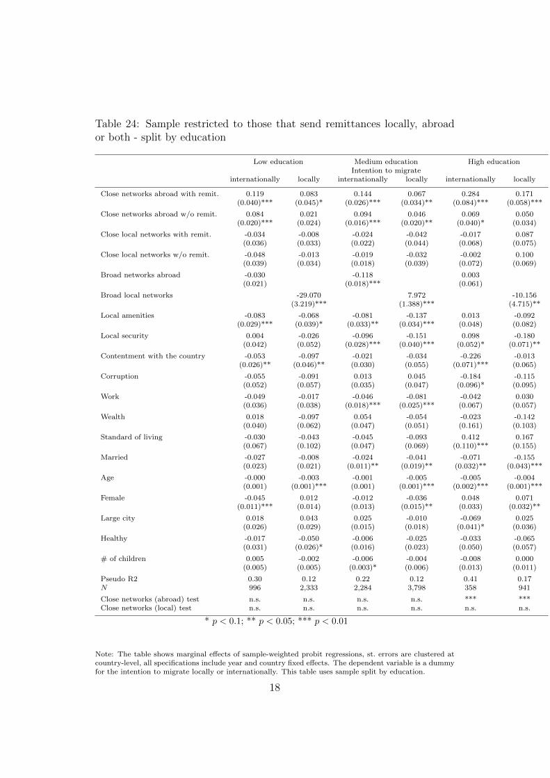
Table 24: Sample restricted to those that send remittances locally, abroador both - split by education

Low education Medium education High educationIntention to migrate

internationally locally internationally locally internationally locally

Close networks abroad with remit. 0.119 0.083 0.144 0.067 0.284 0.171(0.040)*** (0.045)* (0.026)*** (0.034)** (0.084)*** (0.058)***

Close networks abroad w/o remit. 0.084 0.021 0.094 0.046 0.069 0.050(0.020)*** (0.024) (0.016)*** (0.020)** (0.040)* (0.034)

Close local networks with remit. -0.034 -0.008 -0.024 -0.042 -0.017 0.087(0.036) (0.033) (0.022) (0.044) (0.068) (0.075)

Close local networks w/o remit. -0.048 -0.013 -0.019 -0.032 -0.002 0.100(0.039) (0.034) (0.018) (0.039) (0.072) (0.069)

Broad networks abroad -0.030 -0.118 0.003(0.021) (0.018)*** (0.061)

Broad local networks -29.070 7.972 -10.156(3.219)*** (1.388)*** (4.715)**

Local amenities -0.083 -0.068 -0.081 -0.137 0.013 -0.092(0.029)*** (0.039)* (0.033)** (0.034)*** (0.048) (0.082)

Local security 0.004 -0.026 -0.096 -0.151 0.098 -0.180(0.042) (0.052) (0.028)*** (0.040)*** (0.052)* (0.071)**

Contentment with the country -0.053 -0.097 -0.021 -0.034 -0.226 -0.013(0.026)** (0.046)** (0.030) (0.055) (0.071)*** (0.065)

Corruption -0.055 -0.091 0.013 0.045 -0.184 -0.115(0.052) (0.057) (0.035) (0.047) (0.096)* (0.095)

Work -0.049 -0.017 -0.046 -0.081 -0.042 0.030(0.036) (0.038) (0.018)*** (0.025)*** (0.067) (0.057)

Wealth 0.018 -0.097 0.054 -0.054 -0.023 -0.142(0.040) (0.062) (0.047) (0.051) (0.161) (0.103)

Standard of living -0.030 -0.043 -0.045 -0.093 0.412 0.167(0.067) (0.102) (0.047) (0.069) (0.110)*** (0.155)

Married -0.027 -0.008 -0.024 -0.041 -0.071 -0.155(0.023) (0.021) (0.011)** (0.019)** (0.032)** (0.043)***

Age -0.000 -0.003 -0.001 -0.005 -0.005 -0.004(0.001) (0.001)*** (0.001) (0.001)*** (0.002)*** (0.001)***

Female -0.045 0.012 -0.012 -0.036 0.048 0.071(0.011)*** (0.014) (0.013) (0.015)** (0.033) (0.032)**

Large city 0.018 0.043 0.025 -0.010 -0.069 0.025(0.026) (0.029) (0.015) (0.018) (0.041)* (0.036)

Healthy -0.017 -0.050 -0.006 -0.025 -0.033 -0.065(0.031) (0.026)* (0.016) (0.023) (0.050) (0.057)

# of children 0.005 -0.002 -0.006 -0.004 -0.008 0.000(0.005) (0.005) (0.003)* (0.006) (0.013) (0.011)

Pseudo R2 0.30 0.12 0.22 0.12 0.41 0.17N 996 2,333 2,284 3,798 358 941

Close networks (abroad) test n.s. n.s. n.s. n.s. *** ***Close networks (local) test n.s. n.s. n.s. n.s. n.s. n.s.

* p < 0.1; ** p < 0.05; *** p < 0.01

Note: The table shows marginal effects of sample-weighted probit regressions, st. errors are clustered atcountry-level, all specifications include year and country fixed effects. The dependent variable is a dummyfor the intention to migrate locally or internationally. This table uses sample split by education.

18

7 Marginal effects with family abroad

19

Table 25: Marginal effects with family abroad

Linear specifications Non-linear specificationsIntention to migrate

internationally locally internationally locally

Local amenities -0.015 -0.078 -0.015 -0.077(0.007)** (0.027)*** (0.007)** (0.027)***

Local security -0.012 -0.152 -0.013 -0.153(0.017) (0.040)*** (0.017) (0.041)***

Contentment with the country -0.010 -0.018 -0.011 -0.018(0.007) (0.038) (0.007) (0.038)

Corruption -0.015 -0.005 -0.016 -0.006(0.013) (0.032) (0.013) (0.032)

Close local networks -0.020 -0.098 -0.019 -0.098(0.008)** (0.028)*** (0.008)** (0.027)***

Relatives live(d) abroad 0.019 0.019 0.019 0.019(0.006)*** (0.013) (0.005)*** (0.013)

Work 0.008 -0.009 0.007 -0.009(0.006) (0.029) (0.006) (0.029)

Wealth 0.007 -0.122 0.012 -0.115(0.030) (0.053)** (0.032) (0.052)**

Standard of living -0.032 0.003 -0.032 0.009(0.024) (0.062) (0.023) (0.062)

Broad networks abroad 0.027 0.027(0.004)*** (0.004)***

Broad local networks 0.207 0.207(0.016)*** (0.015)***

Married -0.012 -0.002 -0.012 -0.002(0.006)** (0.018) (0.006)** (0.018)

Age -0.001 -0.003 -0.001 -0.004(0.000)*** (0.001)*** (0.000)*** (0.001)***

Education (medium) -0.001 -0.002 0.000 -0.003(0.006) (0.019) (0.007) (0.019)

Education (high) 0.006 0.038 0.006 0.036(0.008) (0.025) (0.008) (0.025)

Female -0.005 -0.020 -0.005 -0.020(0.004) (0.020) (0.004) (0.020)

Large city 0.003 0.020 0.002 0.020(0.006) (0.014) (0.005) (0.014)

Healthy -0.011 -0.028 -0.012 -0.028(0.008) (0.021) (0.008) (0.021)

# of children 0.003 -0.004 0.003 -0.004(0.002) (0.005) (0.002) (0.005)

Pseudo R2 0.20 0.08 0.21 0.08N 3,130 3,846 3,130 3,846

* p < 0.1; ** p < 0.05; *** p < 0.01

Note: The table shows marginal effects of sample-weighted probit regressions, st. errors are clusteredat country-level, all specifications are based on year 2010 only and do not include country fixed effects.The dependent variable is a dummy for the intention to migrate locally or internationally. The first twospecifications include ‘wealth’ and ‘standard of living’ in a linear form, the last two specifications includethese variables and their squared values.

20

8 Variation across regions and country in-

come groups: local migration intentions

This section contains tables for the local migration intention (the correspond-ing tables for international intention are presented in the paper).

Table 26: Results for local migration intention by region

Intention to migrate locallyEurope Ex-USSR Asia Americas MENA Sub-Saharan Africa

Close local networks -0.031 -0.016 -0.003 -0.064 -0.032 -0.022(0.020) (0.019) (0.010) (0.014)*** (0.033) (0.012)*

Close networks abroad 0.029 0.020 0.034 0.045 0.005 0.031(0.009)*** (0.006)*** (0.010)*** (0.009)*** (0.021) (0.009)***

Broad local networks -0.012 0.055 0.104 0.128 0.067 0.174(0.033) (0.038) (0.024)*** (0.047)*** (0.025)*** (0.024)***

Local amenities -0.108 -0.060 -0.121 -0.092 0.002 -0.121(0.021)*** (0.019)*** (0.009)*** (0.017)*** (0.026) (0.020)***

Local security -0.056 -0.001 -0.096 -0.109 -0.144 -0.100(0.025)** (0.024) (0.014)*** (0.018)*** (0.058)** (0.025)***

Contentment with the country 0.017 -0.006 0.030 -0.016 -0.061 -0.050(0.022) (0.017) (0.023) (0.021) (0.038) (0.018)***

Corruption 0.000 0.015 0.033 -0.048 0.014 -0.031(0.025) (0.023) (0.041) (0.021)** (0.053) (0.026)

Work -0.041 -0.037 -0.046 -0.015 -0.035 -0.098(0.010)*** (0.020)* (0.021)** (0.018) (0.028) (0.011)***

Wealth -0.065 0.032 0.023 -0.064 -0.059 0.049(0.029)** (0.030) (0.055) (0.032)** (0.042) (0.025)*

Standard of living 0.018 -0.004 -0.041 0.015 0.145 -0.110(0.030) (0.036) (0.014)*** (0.022) (0.085)* (0.032)***

Married -0.050 -0.019 -0.024 -0.010 -0.031 -0.031(0.009)*** (0.009)** (0.011)** (0.012) (0.021) (0.009)***

Age -0.003 -0.002 -0.002 -0.003 -0.002 -0.004(0.000)*** (0.000)*** (0.000)*** (0.000)*** (0.001)** (0.000)***

Education (medium) 0.012 -0.009 0.012 -0.001 0.018 0.050(0.017) (0.013) (0.007) (0.011) (0.015) (0.009)***

Education (high) 0.034 0.017 0.034 0.030 0.082 0.043(0.019)* (0.019) (0.011)*** (0.013)** (0.029)*** (0.013)***

Female -0.011 0.001 -0.005 -0.009 0.011 -0.029(0.008) (0.007) (0.006) (0.011) (0.037) (0.013)**

Large city 0.000 -0.038 0.020 0.025 0.037 0.001(0.008) (0.008)*** (0.014) (0.011)** (0.022)* (0.010)

Healthy -0.029 -0.014 -0.067 -0.027 -0.003 -0.040(0.016)* (0.010) (0.023)*** (0.016) (0.057) (0.009)***

# of children -0.004 -0.003 -0.001 -0.005 -0.002 -0.000(0.004) (0.004) (0.002) (0.003) (0.002) (0.002)

Pseudo R2 0.13 0.09 0.08 0.07 0.04 0.08N 7,773 4,511 13,709 10,159 1,737 22,644

21

Table 27: Results for local migration intention by income group

Intention to migrate locallyLow income Upper middle income High income

Close local networks -0.024 -0.023 -0.037(0.008)*** (0.014) (0.027)

Close networks abroad 0.029 0.045 0.025(0.006)*** (0.010)*** (0.011)**

Broad local networks 0.106 0.084 0.142(0.017)*** (0.054) (0.051)***

Local amenities -0.116 -0.047 -0.152(0.011)*** (0.017)*** (0.026)***

Local security -0.091 -0.079 -0.072(0.012)*** (0.033)** (0.031)**

Contentment with the country -0.010 -0.033 -0.002(0.016) (0.014)** (0.023)

Corruption -0.009 -0.011 -0.016(0.024) (0.020) (0.026)

Work -0.067 -0.030 -0.040(0.010)*** (0.020) (0.015)***

Wealth 0.033 -0.058 -0.063(0.024) (0.028)** (0.037)*

Standard of living -0.071 0.048 -0.023(0.018)*** (0.027)* (0.040)

Married -0.023 -0.025 -0.054(0.007)*** (0.008)*** (0.014)***

Age -0.003 -0.003 -0.004(0.000)*** (0.000)*** (0.000)***

Education (medium) 0.030 -0.008 -0.027(0.006)*** (0.010) (0.021)

Education (high) 0.038 0.029 0.002(0.008)*** (0.013)** (0.026)

Female -0.019 -0.005 -0.015(0.007)** (0.007) (0.014)

Large city 0.015 -0.005 -0.002(0.008)* (0.010) (0.011)

Healthy -0.045 -0.019 -0.034(0.013)*** (0.015) (0.021)

# of children -0.002 -0.000 -0.010(0.001) (0.004) (0.006)*

Pseudo R2 0.09 0.08 0.12N 43,125 9,884 6,013

22

9 Results with individual income and educa-

tion

This section contains tables for the local migration intention (the correspond-ing tables for international intention are presented in the paper).

Table 28: Intention to migrate locally and individual income levels

Intention to migrate locallyIncome quintile

1–3 4–5

Close networks abroad with remit. 0.069 0.043(0.014)*** (0.013)***

Close networks abroad w/o remit. 0.032 0.023(0.007)*** (0.007)***

Close local networks with remit. -0.024 -0.007(0.012)** (0.013)

Close local networks w/o remit. -0.031 -0.032(0.009)*** (0.011)***

Local broad networks 0.094 0.087(0.020)*** (0.020)***

Close networks abroad test *** n.s.Close local networks n.s. ***Pseudo R2 0.095N 59719

* p < 0.1; ** p < 0.05; *** p < 0.01

Note: The table shows average marginal effects (evaluated at given income quintiles) of sample-weightedprobit regressions, st. errors are clustered at country-level, the specification includes year and countryfixed effects, as well as individual controls (omitted from the table). The dependent variable is a dummyfor the intention to migrate locally. ‘Close networks’ reflect close social ties (local and abroad) of theindividual, while ‘broad networks’ are proxied by log of the number of individuals at the current locationthat would like to move abroad. Close networks (abroad/local) test provides test results if coefficients ofthe two close networks are equal.

23

Table 29: Intention to migrate locally and individual education levels

Intention to migrate locallyLow education Medium education High education

Close networks abroad with remit. 0.041 0.066 0.057(0.016)*** (0.011)*** (0.016)***

Close networks abroad w/o remit. 0.017 0.038 0.024(0.008)** (0.006)*** (0.009)**

Close local networks with remit. -0.014 -0.028 0.018(0.015) (0.012)** (0.023)

Close local networks w/o remit. -0.022 -0.048 -0.006(0.009)** (0.010)*** (0.022)

Local broad networks 0.085 0.101 0.071(0.019)*** (0.020)*** (0.020)***

Close networks abroad test n.s. *** **Close local networks n.s. ** n.s.Pseudo R2 0.096N 59719

* p < 0.1; ** p < 0.05; *** p < 0.01

Note: The table shows average marginal effects (evaluated at given education levels) of sample-weightedprobit regressions, st. errors are clustered at country-level, the specification includes year and countryfixed effects, as well as individual controls (omitted from the table). The dependent variable is a dummyfor the intention to migrate locally. ‘Close networks’ reflect close social ties (local and abroad) of theindividual, while ‘broad networks’ are proxied by log of the number of individuals at the current locationthat would like to move abroad. Close networks (abroad/local) test provides test results if coefficients ofthe two close networks are equal.

24

10 Results with actual migration data for

broad networks abroad

This section contains tables for the international migration intention withlocal broad networks proxied by the log of the migration flows, where the mi-gration flows are obtained using different sources of data: UN, OECD (http://stats.oecd.org/Index.aspx?DataSetCode=MIG), IAB (H. Brucker et al.(2013). “Education, gender and international migration: insights from apanel-dataset 1980-2010”. mimeo).

25

Table 30: PCA index-based results with actual migration data for broadnetworks

Intention to migrate internationallyUN OECD IAB

Close local networks -0.008 -0.008 -0.007(0.004)** (0.004)** (0.004)*

Close networks abroad 0.032 0.034 0.034(0.002)*** (0.002)*** (0.002)***

Broad networks abroad (log unmigrflow) 0.008(0.002)***

Broad networks abroad (log bmigfoecd) 0.012(0.007)*

Broad networks abroad (log iab-bna) -0.058(0.062)

Local amenities -0.030 -0.031 -0.031(0.004)*** (0.004)*** (0.004)***

Local security -0.021 -0.020 -0.020(0.005)*** (0.005)*** (0.005)***

Contentment with the country -0.020 -0.020 -0.021(0.005)*** (0.005)*** (0.005)***

Corruption -0.010 -0.011 -0.012(0.006) (0.006)* (0.006)**

Work -0.018 -0.019 -0.018(0.004)*** (0.003)*** (0.003)***

Wealth 0.008 0.010 0.009(0.006) (0.006)* (0.006)*

Standard of living -0.025 -0.023 -0.024(0.009)*** (0.008)*** (0.008)***

Married -0.013 -0.011 -0.011(0.002)*** (0.002)*** (0.002)***

Age -0.001 -0.001 -0.001(0.000)*** (0.000)*** (0.000)***

Education (medium) 0.006 0.005 0.005(0.003)** (0.003)* (0.003)*

Education (high) 0.015 0.011 0.011(0.004)*** (0.004)*** (0.004)***

Female -0.009 -0.010 -0.010(0.002)*** (0.002)*** (0.002)***

Large city 0.007 0.007 0.007(0.003)** (0.003)** (0.003)**

Healthy -0.010 -0.009 -0.009(0.003)*** (0.003)*** (0.003)***

# of children 0.001 0.001 0.001(0.000)* (0.000)** (0.000)**

Pseudo R2 0.22 0.22 0.22N 45,427 49,001 48,791

Note: broad networks abroad are proxied by the log of the migration flows estimated using UN, OECD

and IAB data.

26

Table 31: Single-question-based results with actual migration data for broadnetworks

Intention to migrate internationallyUN OECD IAB

Close local networks -0.004 -0.003 -0.003(0.002)** (0.002)** (0.002)**

Close networks abroad 0.025 0.026 0.026(0.001)*** (0.001)*** (0.001)***

Broad networks abroad (log unmigrflow) 0.006(0.001)***

Broad networks abroad (log bmigfoecd) 0.003(0.005)

Broad networks abroad (log iab-bna) -0.075(0.040)*

Satisfaction with the city/area -0.029 -0.029 -0.029(0.002)*** (0.002)*** (0.002)***

Country economic condition (getting worse) 0.010 0.009 0.009(0.002)*** (0.002)*** (0.002)***

Country economic condition (getting better) -0.002 -0.002 -0.002(0.002) (0.002) (0.002)

Part-time employment -0.016 -0.015 -0.015(0.002)*** (0.002)*** (0.002)***

Full-time employment -0.012 -0.012 -0.011(0.002)*** (0.002)*** (0.002)***

Log (rel.) income 0.002 0.001 0.001(0.001)** (0.001)* (0.001)*

Married -0.008 -0.007 -0.007(0.001)*** (0.001)*** (0.001)***

Age -0.001 -0.001 -0.001(0.000)*** (0.000)*** (0.000)***

Education (medium) 0.006 0.005 0.005(0.001)*** (0.001)*** (0.001)***

Education (high) 0.013 0.012 0.011(0.002)*** (0.002)*** (0.002)***

Female -0.006 -0.007 -0.006(0.001)*** (0.001)*** (0.001)***

Large city 0.006 0.006 0.006(0.002)*** (0.002)*** (0.002)***

Healthy -0.006 -0.005 -0.005(0.002)*** (0.001)*** (0.001)***

# of children 0.000 0.000 0.000(0.000) (0.000) (0.000)

Pseudo R2 0.24 0.24 0.24N 130,428 142,197 141,596

Note: broad networks abroad are proxied by the log of the migration flows estimated using UN, OECD

and IAB data.

27

11 Results with a stronger intention (includ-

ing preparation)

These tables adjust the dependent variable to incorporate information onwhether the individual has undertaken preparation for a move (a stricterversion of intention than the one used for the main specifications).

Table 32: Index-based results with stronger intention: index-based specifica-tions

Intention to migrate internationally(1) (2)

Close local networks -0.002 -0.005(0.002) (0.002)**

Close networks abroad 0.019 0.016(0.001)*** (0.002)***

Broad networks abroad 0.012 0.012(0.003)*** (0.003)***

Local amenities -0.012 -0.015(0.003)*** (0.003)***

Local security -0.010 -0.008(0.003)*** (0.003)**

Contentment with the country -0.012 -0.008(0.003)*** (0.003)***

Corruption -0.005 -0.005(0.004) (0.004)

Work -0.009 -0.008(0.002)*** (0.002)***

Wealth 0.010 0.001(0.005)** (0.004)

Standard of living -0.010 -0.014(0.007) (0.004)***

Married -0.005 -0.005(0.002)*** (0.001)***

Age -0.000 -0.000(0.000)*** (0.000)***

Education (medium) 0.005 -0.001(0.002)*** (0.002)

Education (high) 0.008 0.002(0.002)*** (0.003)

Female -0.005 -0.004(0.001)*** (0.001)***

Large city 0.003 0.005(0.002) (0.002)**

Healthy -0.005 -0.003(0.002)** (0.002)**

# of children 0.000 0.001(0.000) (0.000)*

Pseudo R2 0.19 0.17N 43,261 55,439

Note: in column (1) the dependent variable is set to 1 only for those cases that actually make preparation

for the move (question wp9455) and observations with inconsistent responses are removed from the sample;

in column (2) the dependent variable is set to 1 only for those cases that actually make preparation for

the move (question wp9455) without checking observations for consistency of their responses.

28

Table 33: Single-question-based results with stronger intention: single-question specifications

Intention to migrate internationally(1) (2)

Close local networks -0.002 -0.002(0.001)* (0.001)*

Close networks abroad 0.016 0.010(0.001)*** (0.001)***

Broad networks abroad 0.007 0.009(0.001)*** (0.001)***

Satisfaction with the city/area -0.014 -0.011(0.002)*** (0.001)***

Country economic condition (getting worse) 0.004 0.004(0.001)*** (0.001)***

Country economic condition (getting better) 0.000 -0.002(0.001) (0.001)**

Part-time employment -0.006 -0.008(0.001)*** (0.001)***

Full-time employment -0.004 -0.006(0.001)*** (0.001)***

Log (rel.) income 0.002 -0.000(0.000)*** (0.000)

Married -0.003 -0.003(0.001)*** (0.001)***

Age -0.000 -0.000(0.000)*** (0.000)***

Education (medium) 0.003 0.002(0.001)*** (0.001)***

Education (high) 0.007 0.002(0.001)*** (0.001)*

Female -0.003 -0.004(0.001)*** (0.001)***

Large city 0.002 0.004(0.001)** (0.001)***

Healthy -0.002 -0.002(0.001)* (0.001)**

# of children -0.000 0.000(0.000) (0.000)

Pseudo R2 0.22 0.19N 131,435 162,198

Note: in column (1) the dependent variable is set to 1 only for those cases that actually make preparation

for the move (question wp9455) and observations with inconsistent responses are removed from the sample;

in column (2) the dependent variable is set to 1 only for those cases that actually make preparation for

the move (question wp9455) without checking observations for consistency of their responses.

12 Sample restricted to country natives only

Tables in this section are based on the sample which is restricted only torespondent born within their country of residence (at the time of survey).

29

Table 34: Index-based results with sample restricted to country natives only

Intention to migrateinternationally locally

Close local networks -0.008 -0.026(0.004)** (0.007)***

Close networks abroad 0.034 0.034(0.003)*** (0.005)***

Broad networks abroad 0.022(0.003)***

Broad local networks 0.109(0.018)***

Local amenities -0.028 -0.103(0.004)*** (0.010)***

Local security -0.018 -0.089(0.005)*** (0.011)***

Contentment with the country -0.021 -0.013(0.005)*** (0.012)

Corruption -0.011 -0.011(0.006)* (0.018)

Work -0.018 -0.056(0.003)*** (0.009)***

Wealth 0.008 0.005(0.005) (0.020)

Standard of living -0.024 -0.047(0.008)*** (0.016)***

Married -0.011 -0.029(0.002)*** (0.005)***

Age -0.001 -0.003(0.000)*** (0.000)***

Education (medium) 0.005 0.022(0.003)* (0.005)***

Education (high) 0.009 0.045(0.004)** (0.007)***

Female -0.009 -0.017(0.002)*** (0.006)***

Large city 0.007 0.009(0.003)** (0.006)

Healthy -0.009 -0.042(0.003)*** (0.010)***

# of children 0.001 -0.002(0.001)* (0.001)

Pseudo R2 0.22 0.10N 46,539 57,786

30

Table 35: Single-question-based results with sample restricted to countrynatives only

Intention to migrateinternationally locally

Close local networks -0.003 -0.014(0.002)** (0.005)**

Close networks abroad 0.026 0.029(0.001)*** (0.003)***

Broad networks abroad 0.016(0.002)***

Broad local networks 0.109(0.007)***

Satisfaction with the city/area -0.028 -0.129(0.002)*** (0.009)***

Country economic condition (getting worse) 0.008 0.013(0.002)*** (0.004)***

Country economic condition (getting better) -0.002 0.008(0.002) (0.004)*

Part-time employment -0.015 -0.046(0.002)*** (0.008)***

Full-time employment -0.010 -0.041(0.002)*** (0.008)***

Log (rel.) income 0.002 0.004(0.001)** (0.002)***

Married -0.007 -0.019(0.001)*** (0.003)***

Age -0.001 -0.002(0.000)*** (0.000)***

Education (medium) 0.006 0.017(0.001)*** (0.003)***

Education (high) 0.010 0.038(0.002)*** (0.005)***

Female -0.006 -0.007(0.001)*** (0.003)**

Large city 0.005 0.013(0.002)*** (0.004)***

Healthy -0.005 -0.023(0.001)*** (0.005)***

# of children 0.000 -0.001(0.000) (0.001)

Pseudo R2 0.24 0.11N 131,784 158,943

* p < 0.1; ** p < 0.05; *** p < 0.01

31

13 Results with lagged peers and country-

year fixed effects

Table 36: Index-based results with lagged peers and country-year fixed effects

Lagged peers Country-year FEIntention to migrate

internationally locally internationally locally

Close local networks -0.007 -0.022 -0.008 -0.026(0.005) (0.007)*** (0.004)** (0.007)***

Close networks abroad 0.038 0.026 0.035 0.033(0.003)*** (0.006)*** (0.002)*** (0.005)***

Broad networks abroad (lag) 0.052(0.010)***

Broad local networks (lag) -0.042(0.009)***

Local amenities -0.037 -0.096 -0.032 -0.105(0.007)*** (0.012)*** (0.004)*** (0.009)***

Local security -0.025 -0.088 -0.021 -0.092(0.005)*** (0.014)*** (0.005)*** (0.011)***

Contentment with the country -0.024 -0.027 -0.020 -0.013(0.008)*** (0.013)** (0.005)*** (0.012)

Corruption -0.018 -0.019 -0.012 -0.008(0.008)** (0.017) (0.006)* (0.018)

Work -0.025 -0.053 -0.019 -0.057(0.006)*** (0.008)*** (0.004)*** (0.009)***

Wealth 0.012 0.010 0.010 0.006(0.008) (0.016) (0.006) (0.019)

Standard of living -0.034 -0.034 -0.025 -0.047(0.013)*** (0.021) (0.009)*** (0.016)***

Married -0.010 -0.029 -0.011 -0.028(0.003)*** (0.007)*** (0.002)*** (0.005)***

Age -0.001 -0.003 -0.001 -0.003(0.000)*** (0.000)*** (0.000)*** (0.000)***

Education (medium) 0.006 0.028 0.006 0.021(0.004) (0.006)*** (0.003)* (0.005)***

Education (high) 0.008 0.047 0.012 0.045(0.005) (0.010)*** (0.004)*** (0.007)***

Female -0.010 -0.018 -0.010 -0.017(0.003)*** (0.005)*** (0.002)*** (0.006)***

Large city 0.008 0.009 0.007 0.007(0.005)* (0.007) (0.003)** (0.006)

Healthy -0.013 -0.036 -0.009 -0.041(0.004)*** (0.008)*** (0.003)*** (0.010)***

# of children -0.000 -0.000 0.001 -0.002(0.001) (0.002) (0.000)* (0.001)

Pseudo R2 0.20 0.09 0.22 0.10N 26,359 34,402 47,265 60,179

* p < 0.1; ** p < 0.05; *** p < 0.01

14 Results with country-year random effects

32

Table 37: Index-based results with country-year random effects

Linear specification Non-linear specificationIntention to migrate

internationally locally internationally locally

Close local networks -0.006 -0.024 -0.006 -0.025(0.002)*** (0.005)*** (0.002)*** (0.005)***

Close networks (abroad) 0.029 0.033 0.029 0.033(0.002)*** (0.003)*** (0.002)*** (0.003)***

Local amenities -0.024 -0.105 -0.024 -0.106(0.003)*** (0.007)*** (0.003)*** (0.007)***

Local security -0.011 -0.079 -0.011 -0.079(0.003)*** (0.007)*** (0.003)*** (0.007)***

Contentment with the country -0.015 -0.003 -0.015 -0.003(0.003)*** (0.006) (0.003)*** (0.006)

Corruption -0.005 -0.006 -0.005 -0.005(0.003)* (0.007) (0.003)* (0.007)

Work -0.016 -0.056 -0.016 -0.056(0.002)*** (0.005)*** (0.002)*** (0.005)***

Wealth 0.003 -0.005 0.002 -0.013(0.003) (0.009) (0.003) (0.009)

Standard of living -0.013 -0.035 -0.013 -0.032(0.004)*** (0.009)*** (0.004)*** (0.009)***

Married -0.010 -0.028 -0.010 -0.028(0.001)*** (0.003)*** (0.001)*** (0.003)***

Age -0.001 -0.003 -0.001 -0.003(0.000)*** (0.000)*** (0.000)*** (0.000)***

Education (medium) 0.003 0.020 0.003 0.019(0.001)** (0.004)*** (0.001)** (0.004)***

Education (high) 0.007 0.038 0.007 0.040(0.002)*** (0.006)*** (0.002)*** (0.006)***

Female -0.006 -0.017 -0.006 -0.017(0.001)*** (0.003)*** (0.001)*** (0.003)***

Large city 0.006 0.015 0.006 0.015(0.001)*** (0.003)*** (0.001)*** (0.003)***

Healthy -0.009 -0.037 -0.009 -0.037(0.002)*** (0.004)*** (0.002)*** (0.004)***

# of children 0.001 -0.002 0.001 -0.002(0.000)*** (0.001)** (0.000)*** (0.001)**

Pseudo R2 . . . .N 51,939 60,533 51,939 60,533

* p < 0.1; ** p < 0.05; *** p < 0.01

33