Center for Service Enterprise Engineering (SEE) ... · Technion - Israel Institute of Technology The William Davidson Faculty of Industrial Engineering and Management Center for Service

Technion - Israel Institute of Technology

The William Davidson Faculty

of Industrial Engineering and Management

Center for Service Enterprise Engineering (SEE)

g/http://ie.technion.ac.il/Labs/Serven

June 2010

1

SEEStat Tutorial

Part 1 ......................................................................................................................................... 2

Example 1.1: Distributions .................................................................................................... 3

Example 1.2: Intraday time series ....................................................................................... 10

Example 1.3: Time series (Daily totals) .............................................................................. 15

Part 2 ....................................................................................................................................... 19

Example 2.1: Distribution fitting. ....................................................................................... 19

Example 2.2: Distribution mixture fitting ........................................................................... 21

Example 2.3: Survival analysis with smoothing of hazard rates......................................... 23

Example 2.4: Smoothing of intraday time series. ............................................................... 25

Part 3 ....................................................................................................................................... 27

Example 3.1: Queue regulated by a protocol (Quick&Railly) ............................................ 27

Example 3.2: Queue length (Business and Platinum). ........................................................ 29

Example 3.3: Average wait time (all) and Unhandled proportion ...................................... 31

Example 3.4: Agents on line ............................................................................................... 33

Example 3.5: Daily flow of Totals calls (Tuesday, April 2, 2002) ..................................... 35

2

Part 1 After connecting to the server, click the SEEStat icon to open the program.

On the top of the screen you see the main menu. Click "Statistical Analysis". We shall work

with "Database Summaries". Click it.

A list-box with names of SEEStat studies appears (two databases in our case). Select

USBank (the database we shall be working with), click "OK" and wait for a few seconds.

Background: The source of this example database is a large call center of a US Bank. This

call center has sites in 4 states. It has about 900-1200 agent positions on weekdays, and 200-

500 agent positions on weekends. Agents process up to 300,000 calls per day. Calls are

queued up, when appropriate, in a central queue; they are then served by agents across sites,

by fitting service types to agent skills.

3

Now you see the “Model” panel.

Example 1.1: Distributions

We shall now create a histogram of the distribution of service time (duration), at 1-second

resolution.

Click the "Distributions" button. Three available distribution- models appear.

Select "Estimates".

4

You see the tab control, that has 4 tabs:

“Variables”, ”Options”, ”Select Categories” and ”X Properties”.

The first one "Variables" is active. This tab is mandatory, which means you must select

variable(s) before moving forward. The three other tabs are optional, which means that they

already have default values.

NOTE: You can select (click) several variables simultaneously by pressing the Ctrl button

and, in parallel, clicking on the variables one by one.

Select "Agent service time"(the last entry in the list).

5

Now click tab "Select Categories". You see a list box with all the service types that are

offered by USBank. Select "Retail", which is the Bank’s main service.

Open the tab "X Properties". It is used to set properties of charts and tables. At the left side

there is a list box "Resolution". The default resolution (bin-size of the histogram) of 5

seconds is marked. Select the minimal resolution 00:01 = 1 second, in order to not miss any

details of the histogram.

Now you must select the dates we focus on. Click button "Dates ->" at the right side.

6

You see the list of months for which the requested data are available.

Select "April 2001".

Below the list of months, you see two options for date-selection (Date type): "Aggregated

days" and "Individual days". "Aggregated days" is a chosen-default, which we now follow.

Click "Days" to make the selection of days, and select "Week days" – an aggregation of all

5 working days of the week. (Holidays and some special days, such as system failure, are

excluded).

7

All selections are have now been completed: click "OK" at the bottom right.

Wait for a few seconds – SEEStat is processing your request: you now see the

chart/histogram, produced as "Sheet 2" within an Excel spreadsheet.

NOTE: All the examples in this tutorial will, from now on, be accumulated in this Excel

file. DO NOT close this Excel file.

Looking at the chart, you see irregularities at the left (near the origin). We will look at these

more carefully later.

USBank Agent service time, Retail

April 2001, Week days

0.0

0.1

0.2

0.3

0.4

0.5

0.6

00:00 01:00 02:00 03:00 04:00 05:00 06:00 07:00 08:00 09:00 10:00 11:00 12:00

Time(mm:ss) (Resolution 1 sec.)

Rela

tive fre

quencie

s %

8

In fact, two sheets have been created: The chart is in “Sheet 2”. "Sheet 1" includes Table(s)

that are associated with the chart, with the default one being "Statistics" table. Click Sheet 1

to see the contents of this table (N=619,082 is the number of observations), then return to

Sheet 2.

Statistics

Agent

service

time

N 619082

N

(average per day) 30954.1

Mean 259.64

Standard

Deviation 275.66

Variance 75989

Median 177

Minimum 0

Maximum 3595

Skewness 3.062

Kurtosis 15.38

Standard

Error Mean 0.35

Interquartile

Range 233

Gini's

Mean Difference NA

Mean

Absolute Deviation 182.95

Median

Absolute

Deviation(MAD) 102

Coefficient

of Variation(CV) (%) 106.17

You can easily make modifications to charts and tables, as long as they do not require the

loading of new data from the database. You will now go through several such modifications.

9

First, return to the SEESTAT main menu by clicking the SEESTAT USBank button, on

the task bar at the lower-left side of the screen – this is a click that you will be exercising

each time that you wish to transfer from Excel to SEEStat.

Click "Excel Chart" on the top main menu at the right; after this click "Modify Chart".

Two tabs are available: "Options" and "Properties". Open "Properties" and change the

resolution to 00:10 = 10 seconds.

Click "OK".

10

USBank Agent service time, Retail


0.0

0.5

1.0

1.5

2.0

2.5

3.0

3.5

00:00 01:00 02:00 03:00 04:00 05:00 06:00 07:00 08:00 09:00 10:00 11:00 12:00 13:00


Rela

tive fre

quencie

s %

The chart is becoming smoother, but at the cost of loosing some details at the left, near the

origin.

Example 1.2: Intraday time series

We now create a chart for arrival-counts to the call center(s) of USBank, during several days

in a September.

First you must return to the "Statistical Models" window. Click the SEESTAT button on

the task bar (left-bottom), next click "Windows" on the main menu (at the top) and select

"Statistical Models"

11

We are now changing models. To this end, select the "New Model" button (bottom-right).

Select now "Time Series" and then select "Intraday".

As in Example 1.1, four tabs appear. In tab “Variable”, select "Arrivals to queue".

12

Now select dates: Click "Dates ->"; Select from "Months" the month of September 2001;

Mark "Individual days", and click the "Days" tab.

.

The list of days contains the date, the name of week-day and comments if any. For example,

Monday, September 3rd, was Labor Day.

It is expected that the Tuesday following a holiday will be a busy day. We thus compare all

Tuesdays of the month: September 4, September 11, September 18 and September 25.

Hold down the “Ctrl” key on the keyboard, and in parallel click, one after one, on the four

Tuesdays of September 2001.

Then click "OK" (bottom right).

13

USBank Arrivals to queue

9:10

0

100

200

300

400

500

600

700

0:00 2:00 4:00 6:00 8:00 10:00 12:00 14:00 16:00 18:00 20:00 22:00

Time (Resolution 5 min.)

Num

ber

of cases

04.09.2001 11.09.2001 18.09.2001 25.09.2001

Note: The graphs appear in “Sheet 4” of Excel. As before,” Sheet 3” contains the

corresponding numerical data.

You see a sharp drop in the number of calls around 09:00 AM on September 11, 2001 –

which of course is not surprising!

You also see that the Tuesday after Labor Day is indeed a heavily-loaded Tuesday, as

anticipated.

The chart is noisy, due to its 5 minute. resolution. We shall momentarily increase the

resolution to 1 hour (60 minutes).We also note the following:

On the two Tuesdays after September 11, the number of calls is low, relative to the Tuesday

after Labor Day. A natural question now arises: Is there a "shape of a Tuesday"? To seek a

common pattern for (the shape of) a Tuesday, if there is any, we change the graphs from

absolute counts to "percent to mean" (mean = average number of calls per resolution

period).

14

Go back to the main menu via the SEESTAT tab (bottom-left). In the main menu select

"Excel Chart" then "Modify Chart". In the "Options" tab, in the “Convert to” table on

the left, select "Percent to mean", and on the “Properties" tab set resolution to 60:00 = 1

hour,

Click "OK".


0

25

50

75

100

125

150

175

200

225

250

275

0:00 2:00 4:00 6:00 8:00 10:00 12:00 14:00 16:00 18:00 20:00 22:00


Perc

ent to

mean

04.09.2001 11.09.2001 18.09.2001 25.09.2001

The "Shape of a Tuesday" is clearly manifested: the distribution of calls over the day is

almost the same for the three Tuesdays, both normal and heavily-loaded. (Surprisingly,

September 11 also catches up from around 13:00 or so.) For example, the arrival rate

during the peak hour – from 10:00-11:00 – is about 2.5 times that of an average hour.

Instead of "Percent to mean", you can plot according to "Proportion to column totals"

which, in simple words, means the "hourly fraction of load".

Going via the “SEESTAT tab”,”Excel Chart”. ”Modify Chart” “Proportions to column

totals”, then “OK”.

15


0

1

2

3

4

5

6

7

8

9

10

11

0:00 2:00 4:00 6:00 8:00 10:00 12:00 14:00 16:00 18:00 20:00 22:00


Pro

port

ion to c

olu

mn tota

ls

04.09.2001 11.09.2001 18.09.2001 25.09.2001

You see that the arrivals during the peak hour 10:00-11:00 constitute 10% of the daily total.

(Such observations make load-predictions much easier: indeed, only the daily total must be

predicted. Once the daily total is determined, the number of arrivals per hour is allocated

according to the shape of the day; e.g. 10% allocated to 10:00-11:00.)

Example 1.3: Time series (Daily totals)

There are two types of daily-totals time-series: individual days during a specific month and

aggregated days by months. We now demonstrate these concepts.

Return to the "Statistical Models" window, via SEESTAT and using "Windows" on the

main menu. Press the "New Model" button. Select "Time Series", then "Daily totals".

16

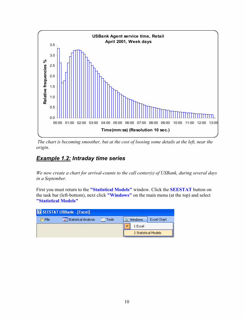
From the variables list select "Arrivals to offered" (around the middle of the list – it counts

arrivals to the phone queue).

Press the "Dates->" button.

Mark "Days for one month" and select (after scrolling down) February 2003.

Open tab "Days" (there is no need for you to select anything, but note the Comments).

Click "OK".

17

USBank Arrivals to offered

February2003

17

12

AbnormalShutdow n

HolidayWeekend

0

10000

20000

30000

40000

50000

60000

70000

80000

1 2 3 4 5 6 7 8 9 10 11 12 13 14 15 16 17 18 19 20 21 22 23 24 25 26 27 28

Days

Num

ber

of cases

Two comments are worth making: On February 12, the system stopped working at 4:00 PM,

and February 17 was a holiday - Washington's birthday. This is manifested on the chart,

where these special days are marked as Abnormal (Shutdown) (green) and Holiday (red).

Note that weekends are also marked (blue).

Return again to the "Statistical Models" window via the SEESTAT tab.

Press button "<-Tables"(middle-right)

From the variables list select "Number of agents".

Open the "Select Categories" tab. Select the following three services: select "Premier"

(priority Retail service), press “Ctrl”, and select "Subanco" (Spanish language),

"Quick&Reilly" (brokerage).

18

Now press the "Dates->" button. Mark "Aggregated days by months" and click "Select

all".

Open the "Days" tab and select "Week days".

Click "OK".

USBank Number of agents

Week days

Nov-02

0

20

40

60

80

100

Mar-01 Jul-01 Nov-01 Mar-02 Jul-02 Nov-02 Mar-03 Jul-03

Month

Avera

ge n

um

ber

of cases

Premier Subanco Quick&Reilly

You see that one of the selected services (Quick&Reilly) was integrated into the Call Center

of USBank only in November 2002.

19

Part 2

Example 2.1: Distribution fitting.

We now fit a parametric service-time distribution to the service-time data from Example 1.1

Open window "Statistical Models". Click "New Model" and select "Distributions" and

"Fitting".

From the variables list select "Agent service time".

Open tab "Options". You see the list of distributions available for fitting.

Mark simultaneously 3 of them: Lognormal, Three-Parameter Lognormal and

Exponential.

Set chart type to "Polygon".

On the tab "Select Categories" select Retail.

Open the “X Properties" tab and set resolution to 00:01 = 1 second.

Click the "Dates->" button. Select April 2001 and “Aggregated days”, open tab "Days"

and select "Week days".

Click "OK".

20

Agent service time

April 2001, Week days Retail

0.00

0.05

0.10

0.15

0.20

0.25

0.30

0.35

0.40

0.45

0.50

0.55

0.60

0.65

00:00 00:30 01:00 01:31 02:01 02:31 03:01 03:32 04:02 04:32 05:02 05:33 06:03 06:33 07:03 07:34 08:04 08:34 09:04 09:35 10:05


Rela

tive fre

quencie

s %

Empirical Lognormal Three-Parameter Lognormal Exponential

Observe again the irregularities near the origin. It looks as though there are at least three

distributions involved: very short calls, abnormally short calls and, after around 30 seconds,

the pattern looks rather regular. The best fit is produced by the Lognormal distribution with

3 parameters, which amounts to a shifted Lognormal curve. But clearly, close the origin from

the right, the fit is inadequate.

You could use the Tables on the previous Sheet (the one accompanying the graph-sheet) to

statistically validate the fit: scroll down until reaching the tables "Parameter-Estimates"

and "Goodness-of-Fit tests".

Distribution Goodness-of-Fit Tests

Residuals

Std

Kolmogorov-Smirnov Cramer-von Mises

Statistic p Value Statistic p Value

Lognormal 0.0471167 0.0823192 <.0001 1374.35 <.0001

Three-Parameter

Lognormal 0.0068412 0.0173089 <.0001 28.97 <.0001

Exponential 0.0338746 0.0659468 <.0001 710.39 <.0001

.

21

Example 2.2: Distribution mixture fitting

We now try to accommodate the behavior to the right of the origin by a mixture of

distributions for “Agent service time”.

Via SEESTAT return to the "Statistical Models" window, click "New Model", select

“Distributions” and "Mixture fitting".

Open the "Options" tab. You cab select a homogeneous or heterogeneous (mixture of

various distributions) option. The former is the default. Select "Lognormal". Set the

number of mixture components to 5, select chart type Polygon.

Click "OK".

22

Fitting Mixtures of Distributions for Agent service time


0.0

0.1

0.2

0.3

0.4

0.5

0.6

0.7

00:00 01:00 02:00 03:00 04:00 05:00 06:00 07:00 08:00 09:00 10:00 11:00 12:00


Rela

tive fre

quencie

s %

Empirical Total Lognormal Lognormal Lognormal Lognormal Lognormal

Fitting Mixtures of Distributions for Agent service time


00:30

0.0

0.1

0.2

0.3

0.4

0.5

0.6

0.7

00:00 00:10 00:20 00:30 00:40 00:50 01:00 01:10 01:19 01:29 01:39 01:49 01:59 02:09


Rela

tive fre

quencie

s %

Empirical Total Lognormal Lognormal Lognormal Lognormal Lognormal

You observe an almost excellent fit (Red line). In particular, on the left side, there are two

components, accommodating the very short and short calls.

23

Going to the previous Excel Sheet, to view the corresponding Tables (by scrolling it down),

one notes that the main component has weight 91% in the mixture – its role in the chart is to

fit the part beyond 30 seconds, which it does very well.

Parameter Estimates

Components Mixing

Proportions

(%)

1. Lognormal 3.08

2. Lognormal 3.58

3. Lognormal 91.14

4. Lognormal 1.86

5. Lognormal 0.34

Example 2.3: Survival analysis with smoothing of hazard rates.

SEEStat supports several survival models. These are required, for example, in order to get

insight into customers' (im)patience, namely the time they are willing to wait prior to

hanging up. Indeed, for those customers who got served, their waiting time provides only a

lower bound on how long they are willing to wait - their (im)patience constitutes censored

observations. One must thus "uncensor" the data to produce adequate estimates. To this end,

we now use a simple survival curve estimate. It will produce hazard-rate functions, which

provide natural statistical summaries of (im)patience.

Return again, via SEESTAT, to the "Statistical Models" window, click "New Model".

Select "Survival analysis" and "Survival Curve Estimate".

24

There are two variable tabs. The first tab "Censored time" is open. Select "Wait time

(handled)": this corresponds to the waiting time of the customers who received service.

Open the "Failure time" and select "Wait time (unhandled)": this corresponds to the

waiting of customers who joined the queue but did not receive service (mainly due to

abandonment, though there are sometimes other reasons such as system malfunction).

Open the "Options" tab. SEEStat supports several methods of smoothing, which are

applicable to hazard rates and beyond.

We shall use the default algorithm (HEFT).

From the tab "Select categories" select "Telesales".

Click "Dates". Select "April 2001" and on the tab "Days" select "Week days".

Click "OK".

25

Survival Analysis

USBank April 2001, Week days, Wait time (unhandled) Telesales,

Hazard Function

0.000

0.005

0.010

0.015

0.020

0.025

0.030

0.035

0.040

0 50 100 150 200 250 300 350 400 450 500 550

Time (seconds)

h(t)

hazard rate Heft 1

A noticeable peak in the hazard rate indicates that there is a trigger for customers to

abandon after about 50 seconds of waiting (which, based on our experience, could be the

result of a voice-announcement at that time).

Example 2.4: Smoothing of intraday time series.

Smoothing algorithms are available for several statistical models. We now demonstrate the

application of smoothing to the data used in Example 1.2.

Return as usual to "Statistical Models", click "New Model", select "Time Series" and

"Intraday". Select "Arrivals to queue". In "Options" tab select “Default” smoothing

(this time, the default is the method of Cubic Splines).

26

Select "Scatter" as chart type

In tab "X Properties", set resolution to 02:00 = 2 minutes.

Click "Dates", mark "Individual days" and select "September 2001".

On the "Days" tab select (with "Ctrl" and click) all four Tuesdays of September.

Press "OK".


0

50

100

150

200

250

300

0:00 2:00 4:00 6:00 8:00 10:00 12:00 14:00 16:00 18:00 20:00 22:00


Num

ber of cases

04.09.2001 11.09.2001 18.09.2001 25.09.2001

04.09.2001 Bspline 11.09.2001 Bspline 18.09.2001 Bspline 25.09.2001 Bspline

For this small resolution of 2 minutes, there is plenty of noise, but the smoothed data clearly

identifies the regular pattern that was discovered before. (Note that the smoothed curves are

computed with the minimal resolution for this variable, which is 30 seconds).

Click "Excel Chart" on the main menu, then click "Modify Chart".

Open the "Properties" tab, set resolution to 15 min. and click "OK".

27


0

250

500

750

1000

1250

1500

1750

2000

2250

0:00 2:00 4:00 6:00 8:00 10:00 12:00 14:00 16:00 18:00 20:00 22:00


Num

ber of cases

04.09.2001 11.09.2001 18.09.2001 25.09.2001

04.09.2001 Bspline 11.09.2001 Bspline 18.09.2001 Bspline 25.09.2001 Bspline

The Averaged Data (over 15 minutes) are now much closer to the smoothed curves, as

expected.

Part 3 Some additional interesting examples.

Example 3.1: Queue regulated by a protocol (Quick&Railly)

Via SEESTAT return to the "Statistical Models" window, click "New Model", then click

the "Distributions" button. Three available distribution models appear. Select "Estimates".

In tab “Variables” select (using Ctrl) both “Wait time (unhandled)” and “Wait time

(handled)”.

In tab “Options” select chart type Polygon. Click “Dates->”, select December 2002, make

sure the "Aggregated days" option is selected, and in "Days" select Week days. Click “<-

Tables”. In “Select Categories” select “Quick&Reilly”. Press "OK".

28

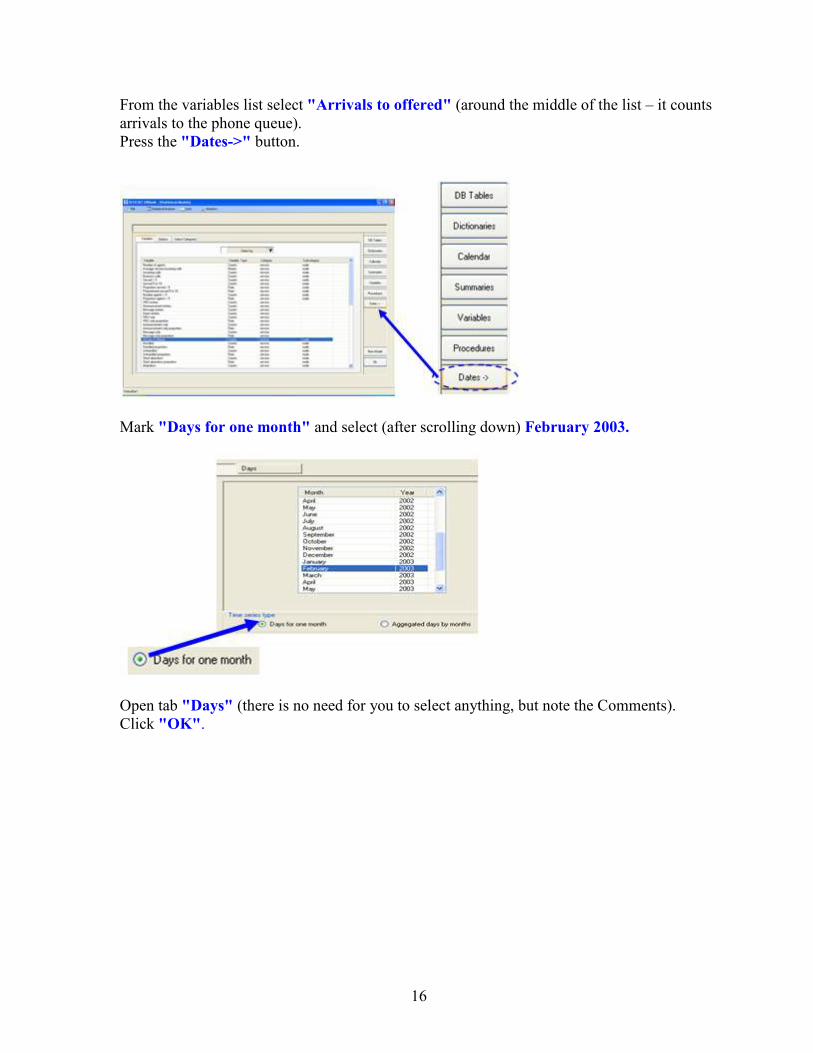
USBank , Quick&Reilly

December 2002, Week days

0

3

6

9

12

15

18

21

24

27

30

00:00 02:00 04:00 06:00 08:00 10:00 12:00 14:00 16:00


Rela

tive fre

quencie

s %

Wait time (unhandled) Wait time (handled)

Both lines are periodical. To get a better focus, you will cut the chart at the left side.

Click "Excel Chart" on the main menu and then "Modify Chart".

Open "Properties", set the low limit 5 seconds.

Click "OK".

29

USBank , Quick&Reilly

December 2002, Week days

0.0

0.5

1.0

1.5

2.0

2.5

3.0

3.5

4.0

4.5

5.0

00:05 02:05 04:05 06:05 08:05 10:05 12:05 14:05 16:05


Rela

tive fre

quencie

s %

Wait time (unhandled) Wait time (handled)

As you see, the Wait time (unhandled), in blue, peaks every 65 sec. The Wait time (handled),

in red, peaks every 130 seconds. These interesting observations are yet to find their

explanations.

Example 3.2: Queue length (Business and Platinum).

Via SEESTAT return to the "Statistical Models" window, click "New Model". Click the

"Time Series" button.

Two available models for time series appear. Select "Intraday". On tab “Variables” select

“Customers in queue (average)”.

On tab “Options” select smoothing “None” and chart type Polygon.

In “Select Categories” tab select (with Ctrl and click) Business and Platinum.

Click “Dates->”, select “Dates totals only”, select the 8 months from May 2002 to

December 2002 and select Week days on the "Days" tab .Click “OK”.

30

USBank Customers in queue (average)

Total for May2002 June2002 July2002 August2002 September2002

October2002 November2002 December2002,Week days

0.0

0.5

1.0

1.5

2.0

2.5

3.0

3.5

4.0

4.5

0:00 2:00 4:00 6:00 8:00 10:00 12:00 14:00 16:00 18:00 20:00 22:00


Avera

ge n

um

ber

of cases

Business Platinum

Platinum is a small-scale service. You will now normalize the chart in order to identify

patters.


Open the "Options" tab and select Percent to mean. Click "OK".

USBank Customers in queue (average)

Total for May2002 June2002 July2002 August2002 September2002

October2002 November2002 December2002,Week days

0

100

200

300

400

500

600

700

800

900

0:00 2:00 4:00 6:00 8:00 10:00 12:00 14:00 16:00 18:00 20:00 22:00


Perc

ent to

mean

Business Platinum

Note the overlapping patterns of the queue lengths of the two customer types. (This

phenomenon is called State-Space-Collapse, in Queueing Theory.)

31

Example 3.3: Average wait time (all) and Unhandled proportion

Via SEESTAT return to the "Statistical Models" window, click "<-Tables". On tab

“Variables” select “Unhandled proportion”. In “Select Categories” tab select “Retail”.

Click “Dates->”, select “April 2001”, and select Week days. Click "OK".

USBank Unhandled proportion, Retail


0

3

6

9

12

15

18

21

24

27

30

0:00 2:00 4:00 6:00 8:00 10:00 12:00 14:00 16:00 18:00 20:00 22:00


Rate

, %

You observe a lot of noise before 8:00 AM. There are only few agents working then, and few

customers are calling. We now cut this irrelevant part of the chart, until 8:00 AM.


Open the "Properties" tab and change low limit to 08:00.

Click "OK".

32

USBank Unhandled proportion, Retail


0

1

2

3

4

5

6

7

8

9

8:00 9:00 10:00 11:00 12:00 13:00 14:00 15:00 16:00 17:00 18:00 19:00 20:00 21:00 22:00 23:00


Rate

, %

Via SEESTAT return to the "Statistical Models" window.

Click "<-Tables". On tab “Variables” select “Average wait time (all)”. Click "OK"

USBank Average wait time(all), Retail


0

5

10

15

20

25

30

35

40

45

8:00 9:00 10:00 11:00 12:00 13:00 14:00 15:00 16:00 17:00 18:00 19:00 20:00 21:00 22:00 23:00


Means

We see that the patterns for two variables ("Unhanded proportion" and Wait Time (all) are

similar. We now compare them more closely.

33

Via SEESTAT return to the "Statistical Models" window. On tab “Variables” select

“Unhandled proportion” and “Average wait time (all)”. Click OK.

USBank , Retail


0

100

200

300

400

500

600

700

8:00 9:00 10:00 11:00 12:00 13:00 14:00 15:00 16:00 17:00 18:00 19:00 20:00 21:00 22:00 23:00


Perc

ent to

mean

Unhandled proportion Average wait time(all)

You observe an increase in "unhandled proportion" and "average wait time" from 17:00 to

20:00. During this period, a lot of agents are leaving their shifts. The number of arrivals is

also going down, but the schedule of agent exits is not synchronized with arrivals – agents

are leaving prematurely. This was a problem for USBank for some period of time.

Example 3.4: Agents on line

Via SEESTAT return to the "Statistical Models" window. On tab “Variable” select

“Agents on line”. In “Select Categories” tab select Retail, Premier, Business and

Consumer Loans. In tab “X Properties” select resolution 10:00 minutes. Click “Dates->”, select April 2001,

Week days. Click OK.

34

USBank Agents on line


0

25

50

75

100

125

150

175

200

225

0:00 2:00 4:00 6:00 8:00 10:00 12:00 14:00 16:00 18:00 20:00 22:00 0:00


Avera

ge n

um

ber

of cases

Retail Premier Business Consumer Loans

Due to the differing volume of services, you will normalize the chart in order to explore the

existence of a common pattern.

Click "Excel Chart" on the main menu and then "Modify Chart”. In tab “Options” select

Percent to mean. Click OK.

USBank Agents on line


0

50

100

150

200

250

300

0:00 2:00 4:00 6:00 8:00 10:00 12:00 14:00 16:00 18:00 20:00 22:00 0:00


Perc

ent to

mean

Retail Premier Business Consumer Loans

35

Example 3.5: Daily flow of Totals calls (Tuesday, April 2, 2002)

Via SEESTAT return to the "Statistical Analysis" menu. Select “Daily Report”.

Click “Dates->”select April 2002, ”Individual days”, click “Days” and select “2 April

2002 Tuesday”. Click OK. (Note; VRU = Voice Response Unit, or simply an Answering

Machine.)

We have chosen a typical day – Tuesday, April 2, 2002 – since this day has virtually no

problematic calls. There is a total of 261,143 calls on that day. The PowerPoint slide

describes the process-flow of calls. There are 4 significant entry points to the system:

through the VRU ~227054 calls (87%), Announcement ~18777 calls, Message ~4517 calls

and Direct group (callers that directly connect to an agent) 2179 calls. 196143 calls (about

79% of all calls) exit from the system through the VRU, Announcement, Message and Others

groups; while another 21% of callers entering the system seek service by an agent (Offered

Volume).

The served callers include those who will request other services 6951 calls (about 13% of the

handled calls), while 46445 calls (86% of callers) exit the system after receiving service by a

single agent.

Documents

Center for Service Enterprise Engineering (SEE) ... · Technion - Israel Institute of Technology The William Davidson Faculty of Industrial Engineering and Management Center for Service