CEP Discussion Paper No 912 March 2009 Government ...eprints.lse.ac.uk/28519/1/dp0912.pdf · Sole-Olle and Sorribas-Navarro (2008) use the same approach as Levitt and Snyder (1997)

CEP Discussion Paper No 912

March 2009

Government Transfers and Political Support

Marco Manacorda, Edward Miguel and Andrea Vigorito

Abstract We estimate the impact of a large anti-poverty program – the Uruguayan PANES – on political support for the government that implemented it. The program mainly consisted of a monthly cash transfer for a period of roughly two and half years. Using the discontinuity in program assignment based on a pre-treatment score, we find that beneficiary households are 21 to 28 percentage points more likely to favor the current government (relative to the previous government). Impacts on political support are larger among poorer households and for those near the center of the political spectrum, consistent with the probabilistic voting model in political economy. Effects persist after the cash transfer program ends. We estimate that the annual cost of increasing government political support by 1 percentage point is roughly 0.9% of annual government social expenditures. Keywords: Conditional cash transfers, redistributive politics, voting, regression discontinuity JEL Classifications: I38, D72 This paper was produced as part of the Centre’s Labour Markets Programme. The Centre for Economic Performance is financed by the Economic and Social Research Council. Acknowledgements We are grateful to Uruguay’s Minister for Social Development, Marina Arismendi and her staff, in particular Marianela Bertoni and Lauro Meléndez at the Monitoring and Evaluation Unit, for making this research possible; to Gabriel Burdín, Adriana Vernengo and James Zuberi for excellent research assistance; and to Verónica Amarante, Gary Becker, David Card, Raj Chetty, Justin McCrary, Gerard Roland, and seminar participants at Columbia University, LSE, U.C. Berkeley ARE, the 2008 Winter Meeting of the NBER Political Economy program, the Universidad de la República (Uruguay), USC, the 2008 CEPR European Summer Symposium in Labor Economics, Stanford, and University of Chicago for comments. Marco Manacorda gratefully acknowledges hospitality from the British Embassy in Montevideo and the Government of Uruguay. Some of the data analyzed in this article were collected by Latinobarómetro Corporation. The Latinobarómetro Corporation is solely responsible for the data distribution and it is not responsible for the views expressed by the users of the data. The authors appreciate the assistance in providing these data. The views expressed in this paper are the authors’ own and do not necessarily reflect those of the Government of Uruguay or the Latinobarómetro Corporation. All errors remain our own. Marco Manacorda is a Research Associate with the Labour Markets Programme at the Centre for Economic Performance, London School of Economics and a Reader in Economics at Queen Mary University, University of London. Edward Miguel is associate professor of economics and director of the Center of Evaluation for Global Action at the University of California, Berkeley. Andrea Vigorito is a Professor in the Department of Economics at the Universidad de la República, Uruguay. Published by Centre for Economic Performance London School of Economics and Political Science Houghton Street London WC2A 2AE All rights reserved. No part of this publication may be reproduced, stored in a retrieval system or transmitted in any form or by any means without the prior permission in writing of the publisher nor be issued to the public or circulated in any form other than that in which it is published. Requests for permission to reproduce any article or part of the Working Paper should be sent to the editor at the above address. © M. Manacorda, E. Miguel and A. Vigorito, submitted 2009 ISBN 978-0-85328-345-4

2

Introduction

Are voters willing to trade-off some of their ideological attachments in exchange for higher

consumption? This is a frequent assumption in leading models of individual voting behavior:

the extent to which voters are willing to trade-off consumption for political ideology

determines politicians’ ability to use transfer programs to capture votes. In the classic

probabilistic voting model (Lindbek and Weibull, 1987, Dixit and Londregan, 1996, 1998,

Persson and Tabellini, 2002), competing parties target transfers to marginal - or “swing” –

voters, i.e., those closest to the centre of the political spectrum, since a one dollar transfer to

this group leads to a greater increase in political support than a transfer to groups with more

extreme ideological attachments. Given the declining marginal utility of consumption, the

model also predicts that a transfer of a given size is also more effective at swaying the

political allegiance of poorer voters. These findings may break down for theoretical reasons

including intertemporal commitment problems (Verdier and Snyder, 2002), “political

machine” dynamics whereby transfers are more effectively targeted to parties’ core

supporters, or risk averse political parties (Cox and McCubbins, 1984).

Despite the central role that voters’ response to government transfers plays in political

economy theory, empirical evidence on the impact of transfers on individual voting behavior

is remarkably scant and rarely based on credible research designs. Identifying the effect of

redistributive politics on individual political preferences is challenging for several reasons.

Most fundamentally, political parties’ tactical considerations, like those described above,

imply that funds are not randomly allocated across voters. For instance, political patronage

strategies could lead parties’ core supporters to be favored by redistribution, i.e., reverse

causality, leading simple OLS regressions of individual political preferences on transfers

received to yield upwardly biased estimates of transfer impacts. Yet the opposite bias could

arise if incumbents, sensing a re-election threat, increased transfers to voters further away

from the party’s base. Even in the absence of tactical spending by parties and politicians,

omitted variables (e.g. household socioeconomic status) might affect both the receipt of

transfers and political preferences, leading to a spurious correlation between the two.

This paper estimates the causal effect of government transfers on political support for

the incumbent party using data from Uruguay. To our knowledge, this is the first paper to

tackle this question using individual level data and a credible source of econometric

identification. In October 2004, against the backdrop of an economic crisis, a center-left

coalition took power in Uruguay for the first time and swiftly introduced a large anti-poverty

3

program, called PANES. The main component of PANES was a conditional cash transfer,

similar to those recently implemented elsewhere in Latin America (including the well-known

Mexican Progresa/Oportunidades program). Household eligibility for the program was

determined by a predicted income score based on a large number of pre-treatment covariates.

Only households with a score below a predetermined threshold were eligible for the program.

Indeed the data show almost perfect enforcement of the assignment rule and we can

confidently rule out manipulation of program assignment on the part of the government.

Eighteen months following the start of the program, households with income scores in

the neighborhood of the threshold were surveyed and asked a series of questions including

their support for the current government. Because assignment to the program near the

threshold was nearly “as good as random”, we are able to circumvent the problems of reverse

causality, endogenous political selection, and omitted variables highlighted above to reliably

estimate the impact of government transfers on political preferences, and thus shed light on

the trade-off between household consumption and political ideology.

In our main empirical finding, the regression discontinuity analysis indicates that

PANES beneficiaries were 21 to 28 percentage points more likely than non-beneficiaries to

favor the current government (relative to the previous one). The result is largely unchanged

across a variety of specifications and with the inclusion of a wide set of household controls.

Back-of-the-envelope calculations suggest that securing one extra supporter costs the

government on the order of US$2,000 per year, or one third of national GDP per capita

(though this estimate is an upper bound cost if political impacts persist after the program has

ended). This implies that a government seeking to increase its vote share by 1 percentage

point would need to increase spending by around 0.9% of total annual government social

expenditures. Uruguay has highly developed democratic political institutions for a middle-

income country, suggesting that some of the political findings could also be relevant for

wealthier countries.

The findings also provide some of the most definitive empirical evidence to date in

support of the leading political economy theories described above, especially in illuminating

the trade-off between consumption and political ideology. In particular, as predicted by the

probabilistic voting model, we find that the effect of government transfers on political

support is significantly larger among poorer households, and among those near the center of

the political spectrum, than among other households.

In the most closely related work, Levitt and Snyder (1997) study the effect of

spending at the district level on voting behavior in the elections for the U.S. House of

4

Representatives. To circumvent the potentially spurious correlation between spending and

voting, they instrument spending in each district with spending in neighboring districts within

the same state. They find a positive effect of non-transfer federal spending on the

incumbent’s vote share, but surprisingly no effect of transfer spending. A possible concern

with their instrumental variable strategy is a violation of the exclusion restriction, for

instance, if spending on roads or military bases in nearby districts directly affect voters’

choices.

Sole-Olle and Sorribas-Navarro (2008) use the same approach as Levitt and Snyder

(1997) – again using aggregate voting data and spending at higher levels of government as an

IV for local spending – and estimate positive impacts of government spending on support for

the incumbent in Spain. Chen (2008a, 2008b) estimates the impact of government transfers

on voting in the United States, and estimates the cost of an additional vote is on the order of

US$7,000. Like us he finds that this cost is increasing in household income but argues that

core supporters are cheaper to buy off, in contrast to our finding. Like Levitt and Snyder

(1997), Chen uses aggregated voting data, rather than the individual level data we prefer, and

finds that there is systematic targeting of government assistance as a function of baseline

voting patterns (with Republican areas favored), complicating the interpretation of his

econometric results, which rely on the quasi-random path of hurricanes to predict federal

government transfers. Green (2006a) uses the discontinuity in assignment to Progresa across

Mexican communities to estimate the effect of the program on voting behavior. She finds a

slightly larger incumbent vote share in treated communities but this pattern is also present

before the program, suggesting endogenous political selection of program beneficiaries rather

than a causal impact there. A related analysis using an observational design and U.S. data is

Markus (1988).1

The paper proceeds as follows. Section I presents a stylized probabilistic model of

voting behavior. Section II presents details of the PANES program and the data. Section III

investigates the effect of the transfer program on political support for the government and

presents some insights into the channels behind the increase in support. The final section

concludes.

1 A related literature explores the implications of voters’ political ideology on political parties’ transfers choices. Dahlberg and Johansson (2002) find support for the swing voter model using the introduction of discretionary funds in Sweden, while others find evidence of core (infra-marginal) voters being disproportionately targeted for redistribution (Case 2000 on Albania, Schady 2002 on Peru, and Green 2006b on Mexico). We focus on the impact of government transfers on voting choices but there is also evidence of direct vote buying in Latin America, including Schaffer (2007) and Stokes (2005).

5

I. THE PROBABILISTIC VOTING MODEL

The standard probabilistic voting model (Lindbeck and Wiebull, 1987; Dixit and Londregan,

1996) is useful for framing the empirical analysis. Consider a governing party (A) that

chooses a schedule of transfers to distribute among citizens. Both A and the opposition party

B have a fixed ideological orientation in the medium-run (a common assumption in these

models), but the transfers they provide to different social groups is a choice variable. For

simplicity, we assume that the transfer schedule of the opposition party B is fixed, for

instance, at what it was when they were last in power, and focus on the policy decisions of

the incumbent party.

Voters differ both in their pre-transfer income, Y, and their underlying ideological

affinities, X. Political affinities are normalized so that a voter with affinity X has a preference

X for the opposition party over the government; thus voters at X=0 are ideologically

indifferent between the two parties. Voters also care about final consumption C, namely, the

sum of their pre-transfer income Y and transfer income T, where the latter can be positive

(subsidies) or negative (taxes).

There are G groups of individuals who can be targeted by government transfers,

indexed by g∈{1, 2, …, G}, where group g has Ng members. Groups can be thought of as

those with certain observable and targetable socio-demographic characteristics (e.g., the

elderly poor living in the capital city). Individuals within each group are allowed to have

heterogeneous political affinities X. The cumulative distribution function of political affinities

for group g is denoted Fg, and the density function is fg. Individuals are indexed by i.

The consumption utility for individuals in group g when the governing party A is in

power is denoted Ug(CAg), with a standard concave function, Ug′>0 and Ug"<0 for all g. CAg is

the sum of pre-transfer income and the transfer chosen for group g. Analogously, individual

consumption utility with the opposition in power is Ug(CBg). Taking into account both final

consumption and political affinities, voter i in group g has a political preference2 for the

governing party iff:

Xig ≤ Ug(Yg + TAg) – Ug(Yg + TBg) ≡ Xg* (1)

2 We follow most of the political economy literature in assuming that voters sincerely express their political preferences in surveys and at the ballot box. With infinitesimal voters, non-truth telling would also be an equilibrium best response but it greatly complicates the analysis.

6

Xg* is the threshold political affinity below which individuals in group g prefer the ruling

party. The total number of voters in group g who support the government, VAg, thus depends

on the distribution of underlying political affinities:

VAg = Ng Fg(Xg*) (2)

The total number of government supporters across all social groups is denoted VA = ΣgVAg.

Now consider the marginal effect of a larger transfer to group g on their political

support for the party in power (A), which has a direct analogue in our empirical analysis:

∂VAg / ∂TAg = fg(Xg*) Ug′(CAg) Ng (3)

Model (1) to (3) provides testable implications for voter behavior in response to

government transfers. The fg term implies that larger transfers translate into more votes when

there is a greater density of voters near the threshold between voting for the government or

the opposition. To illustrate, if the transfer level is already set at so high a level that nearly all

group members already support the government, then a further increase will not yield many

additional votes. Similarly, if the transfer is very low (or negative, i.e., a large tax) and few

group members support the government, then a small transfer increase moves few individuals

close to political indifference. Transfers will thus be most effectively targeted at groups with

many “swing voters”, those groups currently close to the political center for whom small

consumption gains can make a big difference in counteracting political affinities. We

empirically test this implication below by comparing the impact of a government transfer

across social groups with different predicted political affiliations.

The marginal utility Ug′ term, combined with the concavity assumption, implies that a

given transfer has a larger impact for poorer individuals, those at lower levels of pre-transfer

income. This insight might partially explain why political parties in most countries campaign

for some redistribution to the poor independent of their ideological orientation. This

theoretical implication is tested below by examining the interaction between pre-program

income and transfer receipt.

Note finally that the Ng term implies that more votes can be gained by boosting

transfers to larger groups. However, this scale effect drops out once the budget balance

7

condition is considered, since it is also more expensive to increase transfers to all members of

a larger group.3

II. THE PANES PROGRAM IN URUGUAY

Uruguay is a small Latin America country, home to 3.3 million individuals, half of whom live

in the capital of Montevideo. The country experienced rapid economic growth in the first

decades of the twentieth century, and was among the first countries in the region to complete

the demographic transition, implement universal primary education, and establish a generous

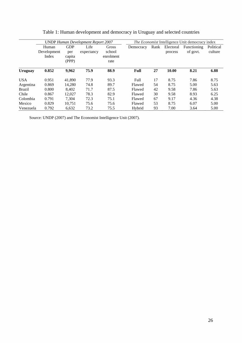
European-style old age pension system. Uruguay is currently among the most developed

Latin American countries according to the UNDP Human Development Index, with strong

life expectancy and schooling indicators (Table 1). According to The Economist Intelligence

Unit, the country’s political system has low levels of corruption, and free and fair elections

(Table 1).4

Economic growth stagnated in the second half of the twentieth century, and the

country went through a severe economic crisis at the start of this decade. Between 2001 and

2002 per capita income fell 11.4%, the poverty rate increased from 18.8% to 23.6%,

unemployment reached its highest level in twenty years (at 17%), the exchange rate

collapsed, and a financial crisis led to bank runs. Currently, PPP-adjusted annual per capita

income is just below US$10,000. The crisis laid bare the weakness of the existing social

safety net, which was largely focused on transfers to the elderly population.5 Yet constrained

in part by a severe fiscal adjustment, the ruling center-right Colorado party government 3 Related models typically use equations (1) to (3) to determine the choice of the optimal transfer schedule in the context of a game between the government and the political opposition. Specifically, the ruling party chooses to set the transfer schedule to maximize its votes VA subject to budget balance condition, Σg{Ng TAg} = 0. This generates an intuitive first order condition, in which the government equates the marginal vote gain from increased transfers across all social groups (taking the policy position of the opposition to be fixed, although the finding generalizes to the strategic game, see Dixit and Londregan, 1996): fg(Xg

*) Ug′(CAg) = λA for all g. We are unable to explore how closely government transfer policies approximate this equilibrium condition in our application since we only have detailed data on a subset of the population, namely, the surveyed households near the PANES program eligibility threshold. This data limitation leads us to restrict our empirical focus to these voters’ responsiveness to the transfer. 4 The Economist ranks Uruguay as one of only two “full democracy” countries in Latin America (the other is Costa Rica). Transparency International ranks Uruguay second only to Chile in the region in terms of perceived control of corruption. The Uruguayan electoral system is presidential with proportional representation in Congress. 5 In 2002, total expenditure on elderly pensions represented 65% of all government social expenditures, 96% of government cash transfers and almost 13% of GDP. This is reflected in marked differences in poverty incidence by age: while nearly half of children under age five lived in poverty that year, the rate for those 65 and older was only 2% (UNDP, 2008).

8

(which had been in power since 1999 in coalition with the Blanco party) focused on

expanding existing programs rather than adopting new measures, with the exception of a

small emergency food plan.

The left-wing Frente Amplio (FA) coalition took power after October 2004 elections,

capitalizing on widespread dissatisfaction with the economy and the previous government’s

management of the crisis. The FA campaigned on a platform that promised extensive

redistribution to the poor and structural economic reforms. The new FA government created

the Ministry for Social Development (Ministerio de Desarrollo Social, MIDES) and swiftly

moved to design and implement the National Social Emergency Plan (Plan de Atención

Nacional a la Emergencia Social), or PANES.

II.a PANES objectives and components

The PANES program was designed to be temporary, running from April 2005 to December

2007, and it had two main aims: first, to provide direct assistance to households who had

experienced a rapid deterioration in living standards since the onset of the 2001-2002 crisis;

and second, and in light of rising poverty during the 1980s and 1990s, to strengthen the

human and social capital of the poor, to enable them to eventually climb out of poverty on

their own.

The PANES target population consisted of the poorest households in the country,

namely the bottom quintile of the income distribution among those falling below the national

poverty line. In all, 102,353 households eventually became program beneficiaries,

approximately 8% of all households (and 10% of the population).

PANES included several distinct components. The largest element was a monthly cash

transfer (ingreso ciudadano, “citizen income”), whose value was set at US$56 (UY$1,360 at

the 2005 exchange rate of US$1=UY$24.43), independent of household size. At US$672 per

year, this is a very large transfer for the target population, amounting to approximately 50%

of average pre-program household self-reported income. Households with children or

pregnant women were also entitled to a food card (tarjeta alimentaria), an in-kind transfer

that operated through an electronic debit card, whose annual value varied between US$156

and US$396. Seventy percent of PANES beneficiaries also received the food card. Additional

but smaller components included public works employment opportunities, job training, and

health care subsidies; more details on PANES are in the appendix.

9

II.b PANES eligibility, enrollment and baseline data

Enrollment of participants occurred in stages. All low income households were publicly

invited to apply and the government also made a large outreach effort, sending enumerators

to poor communities with the intent of boosting applications. Eventually, 188,671 applicant

households were visited by Ministry of Social Development personnel and administered a

baseline survey, providing information on household characteristics, housing, income, work,

and schooling.

To determine assignment to PANES among these applicants, the government used a

predicted income score that depended only on household socioeconomic characteristics

collected in the baseline survey, not directly on income itself. This choice was driven by a

number of factors. First, many households had highly unstable income during the crisis, so

current income was seen as a bad proxy for permanent income. Second, because the target

population often worked in the informal sector, it was difficult to verify their reported income

levels against official social security records, opening up the possibility of misreporting. By

using a wide array of socioeconomic characteristics in the income score, as opposed to self-

reported income, the government hoped to minimize strategic misreporting. The use of a

predicted (as opposed to actual) income score also allows us to estimate heterogeneous

impacts across reported income levels, an advantage of our approach that we elaborate on

below.

The income score was devised by researchers at the University of the Republic

(Universidad de la República), including one of the authors of this paper (Arim et al., 2005),

and was based on a probit model of the likelihood of being above a critical per capita income

level, using a highly saturated function of household variables.6 The model was first

estimated using the 2004 National Household Survey (Encuesta Continua de Hogares). The

resulting coefficient estimates were then used to predict an income score for each applicant

household using PANES baseline survey data. Only households with predicted income scores

below a predetermined threshold were assigned to program treatment.7

6 These included: the type of household (head only; head and spouse; head and children; head, spouse and children only; with non-relatives, with relatives other than head, spouse or children), an indicator for public employees in the household, an indicator for pensioners in the household, average years of education of individuals over age 18 and its square, interactions of age indicators (0-5, 6-17, 18-24, 25-39, 40-54, 45-64, 65 and over) with gender, indicators for household head age, residential overcrowding, whether the household was renting, toilet facilities (no toilet, flush toilet, pit latrine, other) and a wealth index based on durables ownership (e.g., refrigerator, TV, car, etc.). 7 The eligibility thresholds were allowed to vary slightly across the country’s five main administrative regions. The regional thresholds were set to entitle similar shares of poor households in each area to the program. The

10

This discontinuous rule for program assignment was suggested to Ministry officials

by researchers at the University of the Republic and the authors of this paper with the explicit

goal of carrying out the prospective evaluation of PANES. Government officials proved

receptive to the proposal and remarkably uninvolved in the design and calculation of the

eligibility score, which was computed by bureaucrats at the Social Security Administration

(Banco de Previsión Social).8 Similarly, neither the enumerators nor households were ever

informed about the exact variables that entered into the score, the weights attached to them,

or the program eligibility threshold, easing concerns about manipulation of the score.9,10

There was one additional participation condition although in practice it disqualified

only a handful of applicants. Only those households with monthly per capita income below

UY$1,300 (excluding old age pension earnings and any child benefits) could be included in

the program. Hence, the predicted income score was not computed for households with

income exceeding that threshold. All participating households were informed of this rule

before applying.11

The program was fully rolled out within a year of its launch in April 2005. The total

cost of the program by the end of 2007 was US$247,657,026, i.e., US$2,420 per beneficiary

household. On an annual basis, the total is 0.41% of GDP and 1.95% of government social

expenditures. The program was partially financed through a concessionary Inter-American

Development Bank loan.

II.c. Follow-up survey data

regions are: Montevideo, North (Artigas, Salto, Rivera), Center-North (Paysandú, Río Negro, Tacuarembó, Durazno, Treinta y Tres, Cerro Largo), Center-South (Soriano, Florida, Flores, Lavalleja, Rocha) and South (Colonia, San José, Canelones, Maldonado). 8 There was one exception: when officials realized that relatively few one person households would receive program assistance, they asked for a slight adjustment to the predicted income score formula. 9 A relatively small number of households (7,946) were included in the program before September 2005, before the predicted income score was even constructed. An additional 2,552 homeless households were also included in the program irrespective of their score. These households are excluded from the analysis that follows. These households were included in the analysis in an earlier version of this paper, and the main political support results are unchanged. 10 The eligibility score components and weights were made public on the MIDES website only after the program ended (in January 2009). 11 Program participation was also technically contingent on school attendance of all children under age 14 years and regular health checkups for all children and pregnant women, as in many other Latin American conditional cash transfer programs (e.g., Mexico’s PROGRESA). However, we have no record of any households losing PANES benefits for failing to meet these criteria. The cash transfers appear to have been unconditional de facto.

11

The PANES follow-up survey was carried out between December 2006 and March 2007,

roughly eighteen months after the start of the program.12 The questionnaire was designed by

the authors of this paper, in collaboration with Verónica Amarante in the Economics

Department at the University of the Republic, Ministry of Social Development staff, and the

Sociology Department at the University of the Republic. The latter were also in charge of

data collection. To exploit the discontinuity design, the original survey sample contained data

on 3,000 households, including both eligible and ineligible applicants, in the neighborhood of

the program eligibility threshold score. There was a desire to over-represent eligible

households, leading the sample to be split between eligible and ineligible households in a 2:1

ratio.13 The initial non-response rate was moderate at 30%, and replacement households with

approximately the same score as the non-response households were subsequently

interviewed; we discuss the implications of non-response later in the paper. Overall, our

sample contains information on 2,089 households. 14

To limit strategic responses, surveyed households were not informed about the exact

scope of the follow-up survey. Both the title of the survey and information provided to

respondents only referred to the university department and neither made specific mention of

PANES or the Ministry. Questions about the PANES program were asked at the very end of

the questionnaire. In addition to information on housing, household composition, durables

possession, work, income and schooling (as in the baseline survey), the follow-up survey

collected information on health, economic expectations, knowledge of political rights,

participation in social groups, opinions about the PANES program, and political attitudes,

including support for the government, our key outcome variable.

II.d Program implementation

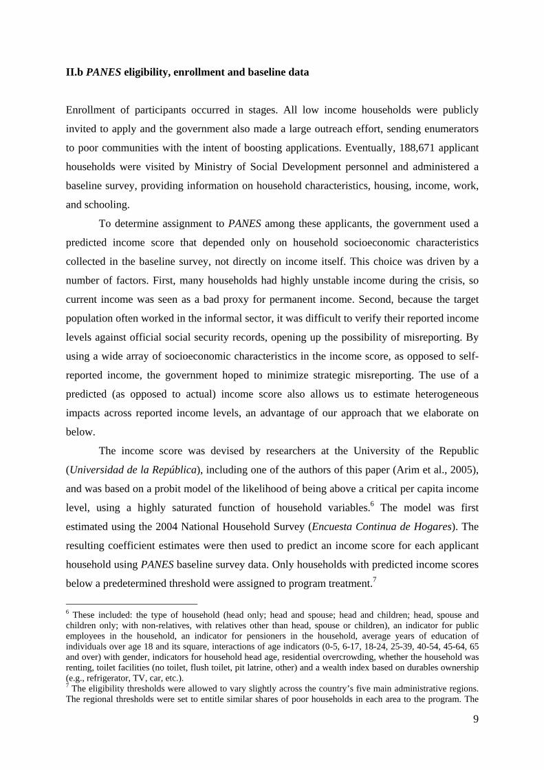
Figure 1 reports the proportion of households who benefited from the program at any point

since its inception, as a function of the baseline predicted income score. The figure is based

on program administrative records. The score was normalized so that all figures are centered

on zero, the eligibility threshold, and such that predicted income increases moving to the right

on the horizontal axis. In this and all subsequent figures (though not in the regression tables) 12 A second follow-up survey with the same households was conducted in early 2008, as we discuss below. 13 This main sample was supplemented with data on 500 eligible households farther away from the eligibility threshold, although we do not use these data in the discontinuity analysis in this paper. 14 We restrict the sample to households that joined the program after September 2005 (and thus for whom inclusion was based on the predicted income score), with baseline social security income below UY$1,300, that were not homeless, and with a valid response to the question on support for the current government.

12

the normalized predicted income score is discretized into intervals. Since there are

approximately twice as many households to the left of the eligibility threshold (i.e., the

PANES eligible households) as to the right, we present twice as many cells for eligible

households (40) as for ineligible ones (20), such that each cell contains approximately the

same number of observations (35 households). These cells thus correspond to equally spaced

percentiles of the score distribution. A linear polynomial on each side of the discontinuity

point is also fit to the data.

The figure demonstrates that program implementation was remarkably clean. Among

applicants practically all potential beneficiaries - i.e., those with a standardized predicted

income score below zero - benefited from the program. The opposite holds for ineligible

households, and the discontinuity in the likelihood of program receipt at the threshold is 98

percentage points. This implies that enforcement of the rule was nearly as strict as implied by

the letter of the law.

Although the program included a variety of components, we do not attempt to

disentangle what roles these different elements played in shaping outcomes since there was

potentially non-random selection into some of them. We concentrate on the overall effect of

program participation at the threshold, which for the vast majority of beneficiary households

consisted solely of the monthly income transfer and the food card.

III. RESULTS

We use the follow-up survey, in conjunction with data from the baseline survey (and the

Latinobarómetro public opinion surveys in some cases) to explore program effects on

political support, the main outcome of interest. We first present average treatment effects, and

then explore heterogeneous treatment effects among groups with different baseline

characteristics. We also test the validity of our identification assumption, namely that

assignment around the eligibility threshold was nearly “as good as random”, as envisioned in

the prospective program evaluation design. A leading concern is manipulation of program

assignment by either officials or enumerators, due to strategic responses, or a correlation

between survey non-response and political views. We also highlight the channels through

which the program affects attitudes by investigating respondents’ post-program income, as

well as subjective assessments of their own well-being and the country’s current situation.

13

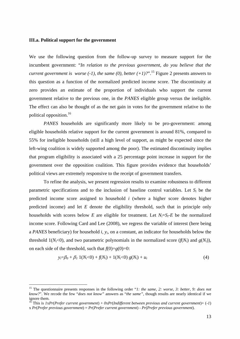
III.a. Political support for the government

We use the following question from the follow-up survey to measure support for the

incumbent government: “In relation to the previous government, do you believe that the

current government is worse (-1), the same (0), better (+1)?”.15 Figure 2 presents answers to

this question as a function of the normalized predicted income score. The discontinuity at

zero provides an estimate of the proportion of individuals who support the current

government relative to the previous one, in the PANES eligible group versus the ineligible.

The effect can also be thought of as the net gain in votes for the government relative to the

political opposition.16

PANES households are significantly more likely to be pro-government: among

eligible households relative support for the current government is around 81%, compared to

55% for ineligible households (still a high level of support, as might be expected since the

left-wing coalition is widely supported among the poor). The estimated discontinuity implies

that program eligibility is associated with a 25 percentage point increase in support for the

government over the opposition coalition. This figure provides evidence that households’

political views are extremely responsive to the receipt of government transfers.

To refine the analysis, we present regression results to examine robustness to different

parametric specifications and to the inclusion of baseline control variables. Let Si be the

predicted income score assigned to household i (where a higher score denotes higher

predicted income) and let E denote the eligibility threshold, such that in principle only

households with scores below E are eligible for treatment. Let Ni=Si-E be the normalized

income score. Following Card and Lee (2008), we regress the variable of interest (here being

a PANES beneficiary) for household i, yi, on a constant, an indicator for households below the

threshold 1(Ni<0), and two parametric polynomials in the normalized score (f(Ni) and g(Ni)),

on each side of the threshold, such that f(0)=g(0)=0:

yi=β0 + β1 1(Ni<0) + f(Ni) + 1(Ni<0) g(Ni) + ui (4)

15 The questionnaire presents responses in the following order “1: the same, 2: worse, 3: better, 9: does not know?”. We recode the few “does not know” answers as “the same”, though results are nearly identical if we ignore them. 16 This is 1xPr(Prefer current government) + 0xPr(Indifferent between previous and current government)+ (-1) x Pr(Prefer previous government) = Pr(Prefer current government) - Pr(Prefer previous government).

14

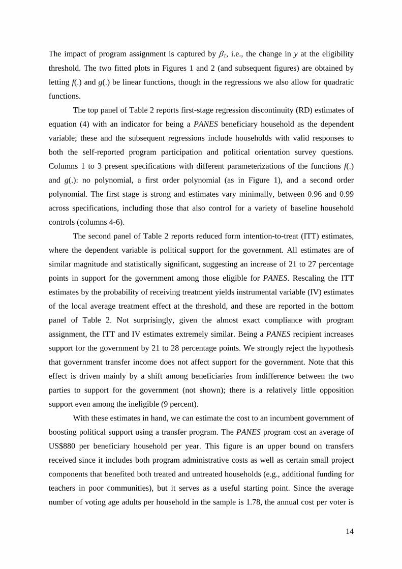
The impact of program assignment is captured by β1, i.e., the change in y at the eligibility

threshold. The two fitted plots in Figures 1 and 2 (and subsequent figures) are obtained by

letting f(.) and g(.) be linear functions, though in the regressions we also allow for quadratic

functions.

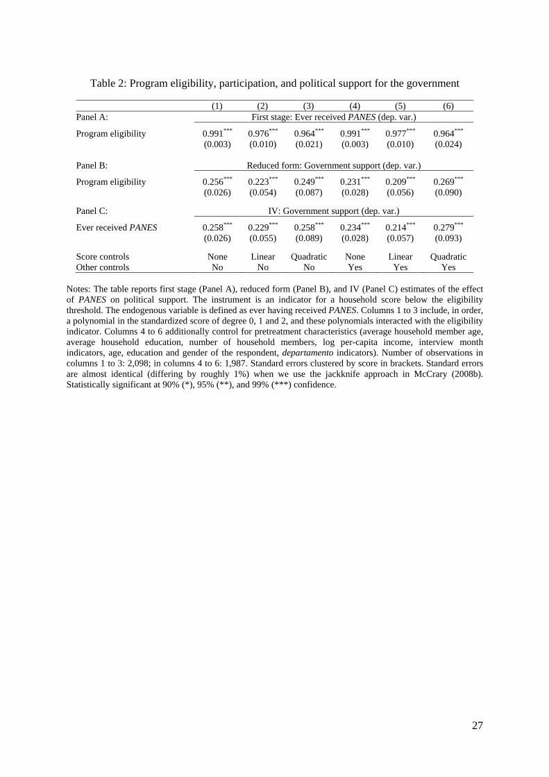
The top panel of Table 2 reports first-stage regression discontinuity (RD) estimates of

equation (4) with an indicator for being a PANES beneficiary household as the dependent

variable; these and the subsequent regressions include households with valid responses to

both the self-reported program participation and political orientation survey questions.

Columns 1 to 3 present specifications with different parameterizations of the functions f(.)

and g(.): no polynomial, a first order polynomial (as in Figure 1), and a second order

polynomial. The first stage is strong and estimates vary minimally, between 0.96 and 0.99

across specifications, including those that also control for a variety of baseline household

controls (columns 4-6).

The second panel of Table 2 reports reduced form intention-to-treat (ITT) estimates,

where the dependent variable is political support for the government. All estimates are of

similar magnitude and statistically significant, suggesting an increase of 21 to 27 percentage

points in support for the government among those eligible for PANES. Rescaling the ITT

estimates by the probability of receiving treatment yields instrumental variable (IV) estimates

of the local average treatment effect at the threshold, and these are reported in the bottom

panel of Table 2. Not surprisingly, given the almost exact compliance with program

assignment, the ITT and IV estimates extremely similar. Being a PANES recipient increases

support for the government by 21 to 28 percentage points. We strongly reject the hypothesis

that government transfer income does not affect support for the government. Note that this

effect is driven mainly by a shift among beneficiaries from indifference between the two

parties to support for the government (not shown); there is a relatively little opposition

support even among the ineligible (9 percent).

With these estimates in hand, we can estimate the cost to an incumbent government of

boosting political support using a transfer program. The PANES program cost an average of

US$880 per beneficiary household per year. This figure is an upper bound on transfers

received since it includes both program administrative costs as well as certain small project

components that benefited both treated and untreated households (e.g., additional funding for

teachers in poor communities), but it serves as a useful starting point. Since the average

number of voting age adults per household in the sample is 1.78, the annual cost per voter is

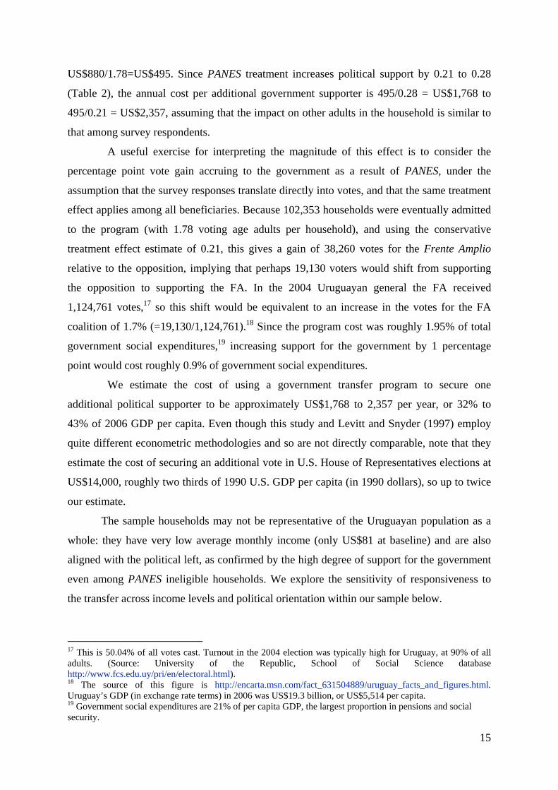
15

US$880/1.78=US$495. Since PANES treatment increases political support by 0.21 to 0.28

(Table 2), the annual cost per additional government supporter is 495/0.28 = US$1,768 to

495/0.21 = US$2,357, assuming that the impact on other adults in the household is similar to

that among survey respondents.

A useful exercise for interpreting the magnitude of this effect is to consider the

percentage point vote gain accruing to the government as a result of PANES, under the

assumption that the survey responses translate directly into votes, and that the same treatment

effect applies among all beneficiaries. Because 102,353 households were eventually admitted

to the program (with 1.78 voting age adults per household), and using the conservative

treatment effect estimate of 0.21, this gives a gain of 38,260 votes for the Frente Amplio

relative to the opposition, implying that perhaps 19,130 voters would shift from supporting

the opposition to supporting the FA. In the 2004 Uruguayan general the FA received

1,124,761 votes,17 so this shift would be equivalent to an increase in the votes for the FA

coalition of 1.7% (=19,130/1,124,761).18 Since the program cost was roughly 1.95% of total

government social expenditures,19 increasing support for the government by 1 percentage

point would cost roughly 0.9% of government social expenditures.

We estimate the cost of using a government transfer program to secure one

additional political supporter to be approximately US$1,768 to 2,357 per year, or 32% to

43% of 2006 GDP per capita. Even though this study and Levitt and Snyder (1997) employ

quite different econometric methodologies and so are not directly comparable, note that they

estimate the cost of securing an additional vote in U.S. House of Representatives elections at

US$14,000, roughly two thirds of 1990 U.S. GDP per capita (in 1990 dollars), so up to twice

our estimate.

The sample households may not be representative of the Uruguayan population as a

whole: they have very low average monthly income (only US$81 at baseline) and are also

aligned with the political left, as confirmed by the high degree of support for the government

even among PANES ineligible households. We explore the sensitivity of responsiveness to

the transfer across income levels and political orientation within our sample below.

17 This is 50.04% of all votes cast. Turnout in the 2004 election was typically high for Uruguay, at 90% of all adults. (Source: University of the Republic, School of Social Science database http://www.fcs.edu.uy/pri/en/electoral.html). 18 The source of this figure is http://encarta.msn.com/fact_631504889/uruguay_facts_and_figures.html. Uruguay’s GDP (in exchange rate terms) in 2006 was US$19.3 billion, or US$5,514 per capita. 19 Government social expenditures are 21% of per capita GDP, the largest proportion in pensions and social security.

16

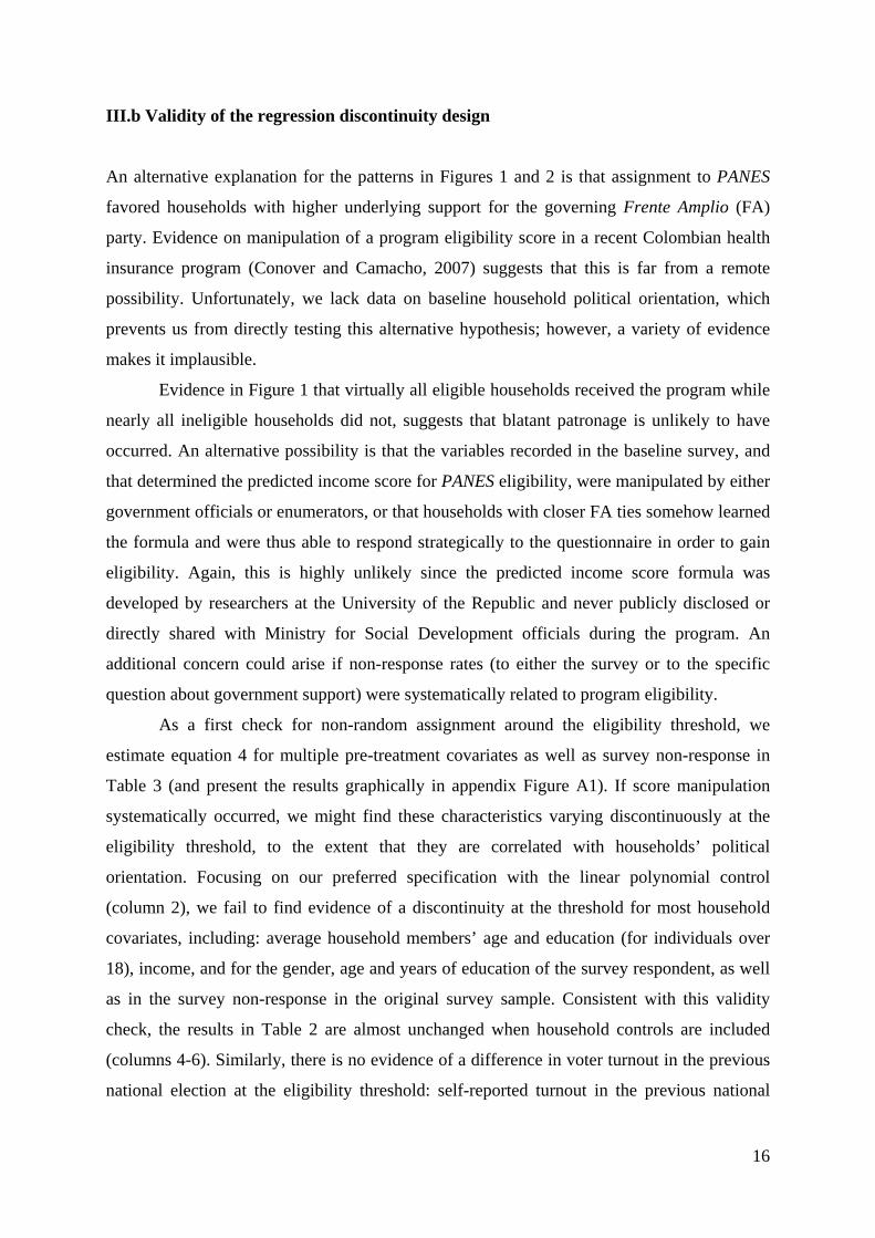
III.b Validity of the regression discontinuity design

An alternative explanation for the patterns in Figures 1 and 2 is that assignment to PANES

favored households with higher underlying support for the governing Frente Amplio (FA)

party. Evidence on manipulation of a program eligibility score in a recent Colombian health

insurance program (Conover and Camacho, 2007) suggests that this is far from a remote

possibility. Unfortunately, we lack data on baseline household political orientation, which

prevents us from directly testing this alternative hypothesis; however, a variety of evidence

makes it implausible.

Evidence in Figure 1 that virtually all eligible households received the program while

nearly all ineligible households did not, suggests that blatant patronage is unlikely to have

occurred. An alternative possibility is that the variables recorded in the baseline survey, and

that determined the predicted income score for PANES eligibility, were manipulated by either

government officials or enumerators, or that households with closer FA ties somehow learned

the formula and were thus able to respond strategically to the questionnaire in order to gain

eligibility. Again, this is highly unlikely since the predicted income score formula was

developed by researchers at the University of the Republic and never publicly disclosed or

directly shared with Ministry for Social Development officials during the program. An

additional concern could arise if non-response rates (to either the survey or to the specific

question about government support) were systematically related to program eligibility.

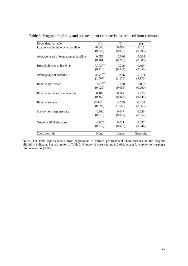
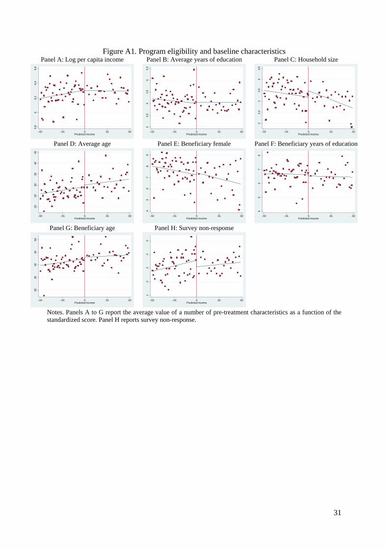
As a first check for non-random assignment around the eligibility threshold, we

estimate equation 4 for multiple pre-treatment covariates as well as survey non-response in

Table 3 (and present the results graphically in appendix Figure A1). If score manipulation

systematically occurred, we might find these characteristics varying discontinuously at the

eligibility threshold, to the extent that they are correlated with households’ political

orientation. Focusing on our preferred specification with the linear polynomial control

(column 2), we fail to find evidence of a discontinuity at the threshold for most household

covariates, including: average household members’ age and education (for individuals over

18), income, and for the gender, age and years of education of the survey respondent, as well

as in the survey non-response in the original survey sample. Consistent with this validity

check, the results in Table 2 are almost unchanged when household controls are included

(columns 4-6). Similarly, there is no evidence of a difference in voter turnout in the previous

national election at the eligibility threshold: self-reported turnout in the previous national

17

election was 93% for both eligible and ineligible households, in line with the consistently

high turnout in Uruguay, where voting is mandatory.

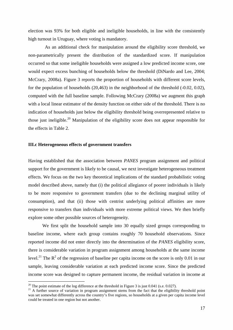
As an additional check for manipulation around the eligibility score threshold, we

non-parametrically present the distribution of the standardized score. If manipulation

occurred so that some ineligible households were assigned a low predicted income score, one

would expect excess bunching of households below the threshold (DiNardo and Lee, 2004;

McCrary, 2008a). Figure 3 reports the proportion of households with different score levels,

for the population of households (20,463) in the neighborhood of the threshold (-0.02, 0.02),

computed with the full baseline sample. Following McCrary (2008a) we augment this graph

with a local linear estimator of the density function on either side of the threshold. There is no

indication of households just below the eligibility threshold being overrepresented relative to

those just ineligible.20 Manipulation of the eligibility score does not appear responsible for

the effects in Table 2.

III.c Heterogeneous effects of government transfers

Having established that the association between PANES program assignment and political

support for the government is likely to be causal, we next investigate heterogeneous treatment

effects. We focus on the two key theoretical implications of the standard probabilistic voting

model described above, namely that (i) the political allegiance of poorer individuals is likely

to be more responsive to government transfers (due to the declining marginal utility of

consumption), and that (ii) those with centrist underlying political affinities are more

responsive to transfers than individuals with more extreme political views. We then briefly

explore some other possible sources of heterogeneity.

We first split the household sample into 30 equally sized groups corresponding to

baseline income, where each group contains roughly 70 household observations. Since

reported income did not enter directly into the determination of the PANES eligibility score,

there is considerable variation in program assignment among households at the same income

level.21 The R2 of the regression of baseline per capita income on the score is only 0.01 in our

sample, leaving considerable variation at each predicted income score. Since the predicted

income score was designed to capture permanent income, the residual variation in income at 20 The point estimate of the log difference at the threshold in Figure 3 is just 0.041 (s.e. 0.027). 21 A further source of variation in program assignment stems from the fact that the eligibility threshold point was set somewhat differently across the country’s five regions, so households at a given per capita income level could be treated in one region but not another.

18

a given score can be thought of as temporary income shocks (e.g., due to job loss) as well as

prediction and measurement error. The extensive variation in reported income at each

predicted income level allows us to estimate heterogeneous impacts across a wide range of

income levels, a strength of our empirical setting.

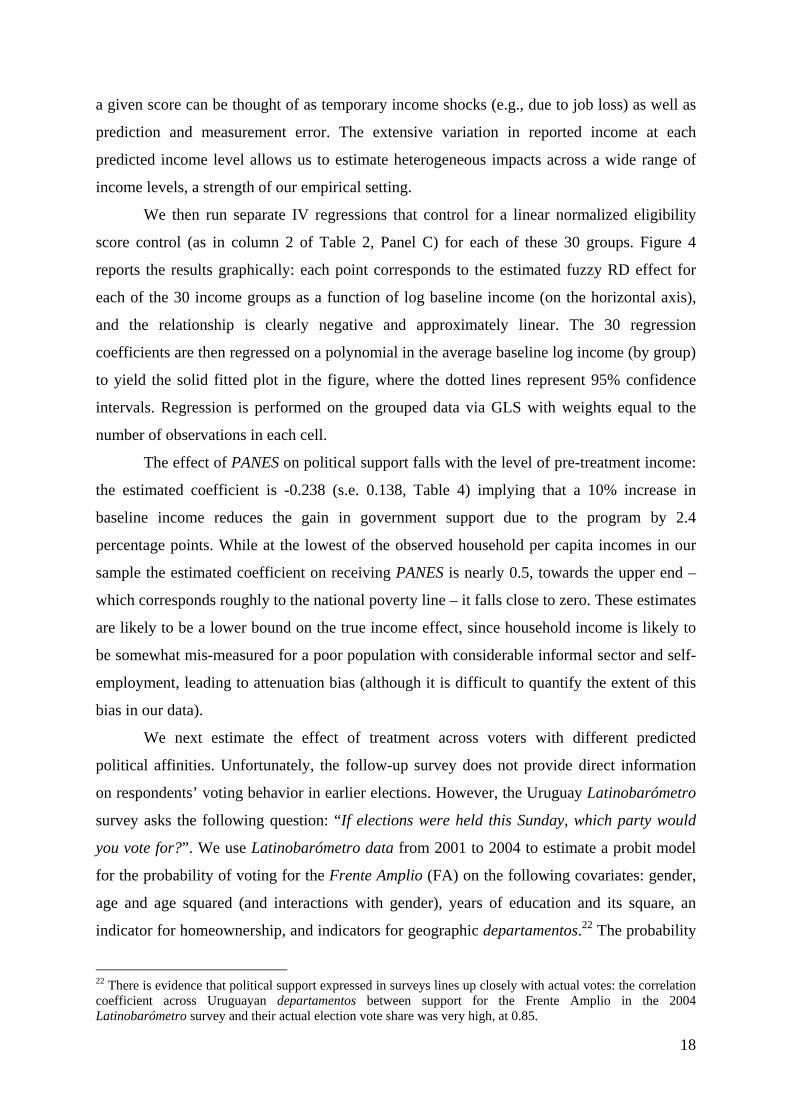
We then run separate IV regressions that control for a linear normalized eligibility

score control (as in column 2 of Table 2, Panel C) for each of these 30 groups. Figure 4

reports the results graphically: each point corresponds to the estimated fuzzy RD effect for

each of the 30 income groups as a function of log baseline income (on the horizontal axis),

and the relationship is clearly negative and approximately linear. The 30 regression

coefficients are then regressed on a polynomial in the average baseline log income (by group)

to yield the solid fitted plot in the figure, where the dotted lines represent 95% confidence

intervals. Regression is performed on the grouped data via GLS with weights equal to the

number of observations in each cell.

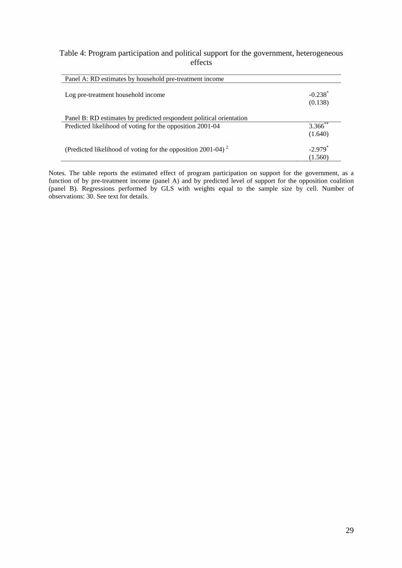
The effect of PANES on political support falls with the level of pre-treatment income:

the estimated coefficient is -0.238 (s.e. 0.138, Table 4) implying that a 10% increase in

baseline income reduces the gain in government support due to the program by 2.4

percentage points. While at the lowest of the observed household per capita incomes in our

sample the estimated coefficient on receiving PANES is nearly 0.5, towards the upper end –

which corresponds roughly to the national poverty line – it falls close to zero. These estimates

are likely to be a lower bound on the true income effect, since household income is likely to

be somewhat mis-measured for a poor population with considerable informal sector and self-

employment, leading to attenuation bias (although it is difficult to quantify the extent of this

bias in our data).

We next estimate the effect of treatment across voters with different predicted

political affinities. Unfortunately, the follow-up survey does not provide direct information

on respondents’ voting behavior in earlier elections. However, the Uruguay Latinobarómetro

survey asks the following question: “If elections were held this Sunday, which party would

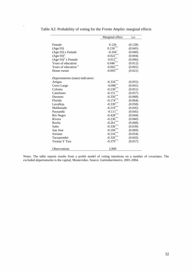
you vote for?”. We use Latinobarómetro data from 2001 to 2004 to estimate a probit model

for the probability of voting for the Frente Amplio (FA) on the following covariates: gender,

age and age squared (and interactions with gender), years of education and its square, an

indicator for homeownership, and indicators for geographic departamentos.22 The probability

22 There is evidence that political support expressed in surveys lines up closely with actual votes: the correlation coefficient across Uruguayan departamentos between support for the Frente Amplio in the 2004 Latinobarómetro survey and their actual election vote share was very high, at 0.85.

19

of voting for the FA increases with age, peaking at around age 40 and then declining

(appendix Table A2), while education is positively associated with being left-leaning, and

gender differences appear minor. There are large and significant differences across

departamentos, and predicted support ranges widely, between roughly 20% and 80%. We use

this model to predict pre-program political orientations for sample households, using the

same covariates available in the PANES baseline survey. Then using a procedure analogous

to that used across income groups, we estimate heterogeneous effects of PANES treatment

across individuals with different predicted pre-program political support for the government.

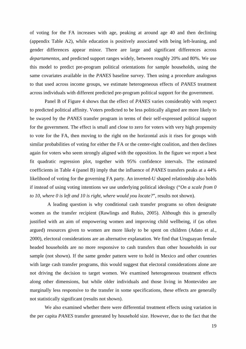
Panel B of Figure 4 shows that the effect of PANES varies considerably with respect

to predicted political affinity. Voters predicted to be less politically aligned are more likely to

be swayed by the PANES transfer program in terms of their self-expressed political support

for the government. The effect is small and close to zero for voters with very high propensity

to vote for the FA, then moving to the right on the horizontal axis it rises for groups with

similar probabilities of voting for either the FA or the center-right coalition, and then declines

again for voters who seem strongly aligned with the opposition. In the figure we report a best

fit quadratic regression plot, together with 95% confidence intervals. The estimated

coefficients in Table 4 (panel B) imply that the influence of PANES transfers peaks at a 44%

likelihood of voting for the governing FA party. An inverted-U shaped relationship also holds

if instead of using voting intentions we use underlying political ideology (“On a scale from 0

to 10, where 0 is left and 10 is right, where would you locate?”, results not shown).

A leading question is why conditional cash transfer programs so often designate

women as the transfer recipient (Rawlings and Rubio, 2005). Although this is generally

justified with an aim of empowering women and improving child wellbeing, if (as often

argued) resources given to women are more likely to be spent on children (Adato et al.,

2000), electoral considerations are an alternative explanation. We find that Uruguayan female

headed households are no more responsive to cash transfers than other households in our

sample (not shown). If the same gender pattern were to hold in Mexico and other countries

with large cash transfer programs, this would suggest that electoral considerations alone are

not driving the decision to target women. We examined heterogeneous treatment effects

along other dimensions, but while older individuals and those living in Montevideo are

marginally less responsive to the transfer in some specifications, these effects are generally

not statistically significant (results not shown).

We also examined whether there were differential treatment effects using variation in

the per capita PANES transfer generated by household size. However, due to the fact that the

20

food card transfer increases with the number of children in the household, and larger

households are also more likely to receive additional benefits from smaller program

components, there is insufficient variation in per capita transfers to draw firm conclusions

(results not shown).

III.d Income and labor market impacts and other channels explaining political support

The estimates in the previous sections show a large increase in support for the government

among households that received the PANES transfer program. The next question is why. The

theoretical model in section I links voting to utility, or well-being, so we would expect

PANES program households to claim to be better-off overall.

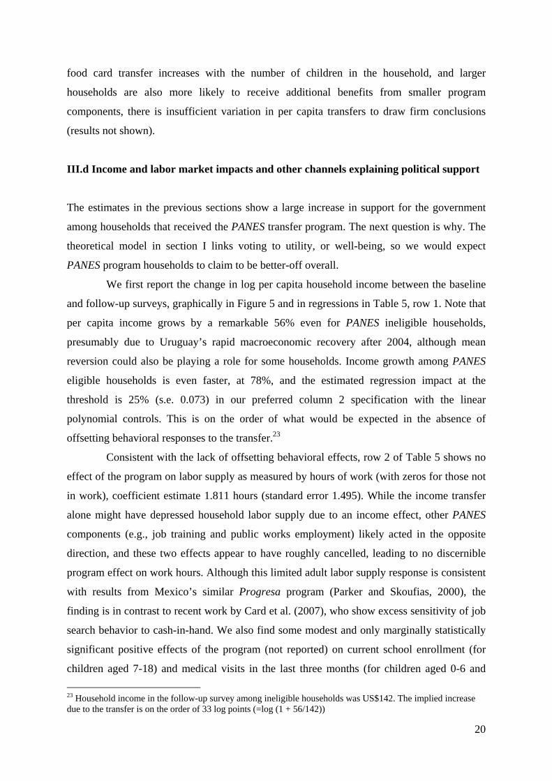
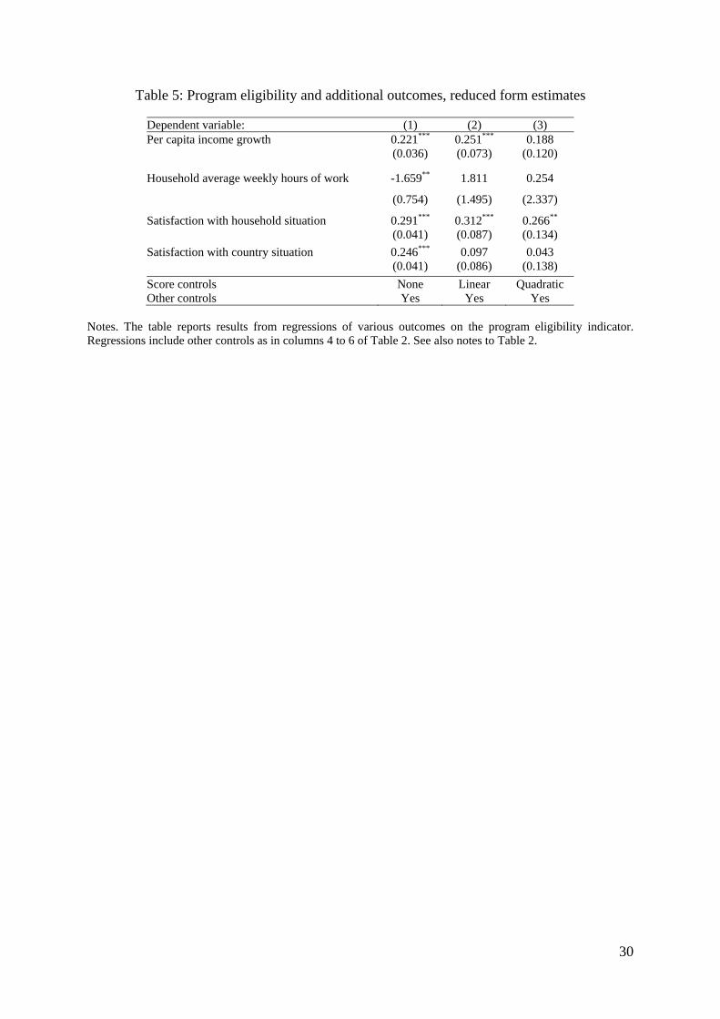
We first report the change in log per capita household income between the baseline

and follow-up surveys, graphically in Figure 5 and in regressions in Table 5, row 1. Note that

per capita income grows by a remarkable 56% even for PANES ineligible households,

presumably due to Uruguay’s rapid macroeconomic recovery after 2004, although mean

reversion could also be playing a role for some households. Income growth among PANES

eligible households is even faster, at 78%, and the estimated regression impact at the

threshold is 25% (s.e. 0.073) in our preferred column 2 specification with the linear

polynomial controls. This is on the order of what would be expected in the absence of

offsetting behavioral responses to the transfer.23

Consistent with the lack of offsetting behavioral effects, row 2 of Table 5 shows no

effect of the program on labor supply as measured by hours of work (with zeros for those not

in work), coefficient estimate 1.811 hours (standard error 1.495). While the income transfer

alone might have depressed household labor supply due to an income effect, other PANES

components (e.g., job training and public works employment) likely acted in the opposite

direction, and these two effects appear to have roughly cancelled, leading to no discernible

program effect on work hours. Although this limited adult labor supply response is consistent

with results from Mexico’s similar Progresa program (Parker and Skoufias, 2000), the

finding is in contrast to recent work by Card et al. (2007), who show excess sensitivity of job

search behavior to cash-in-hand. We also find some modest and only marginally statistically

significant positive effects of the program (not reported) on current school enrollment (for

children aged 7-18) and medical visits in the last three months (for children aged 0-6 and 23 Household income in the follow-up survey among ineligible households was US$142. The implied increase due to the transfer is on the order of 33 log points (=log (1 + 56/142))

21

women of childbearing age, 14-35), perhaps due to the conditions officially attached to

program receipt, which may have swayed some households. However, there is no evidence of

impacts on durables ownership, home characteristics or self-reported health (Amarante et al.,

2008). 24

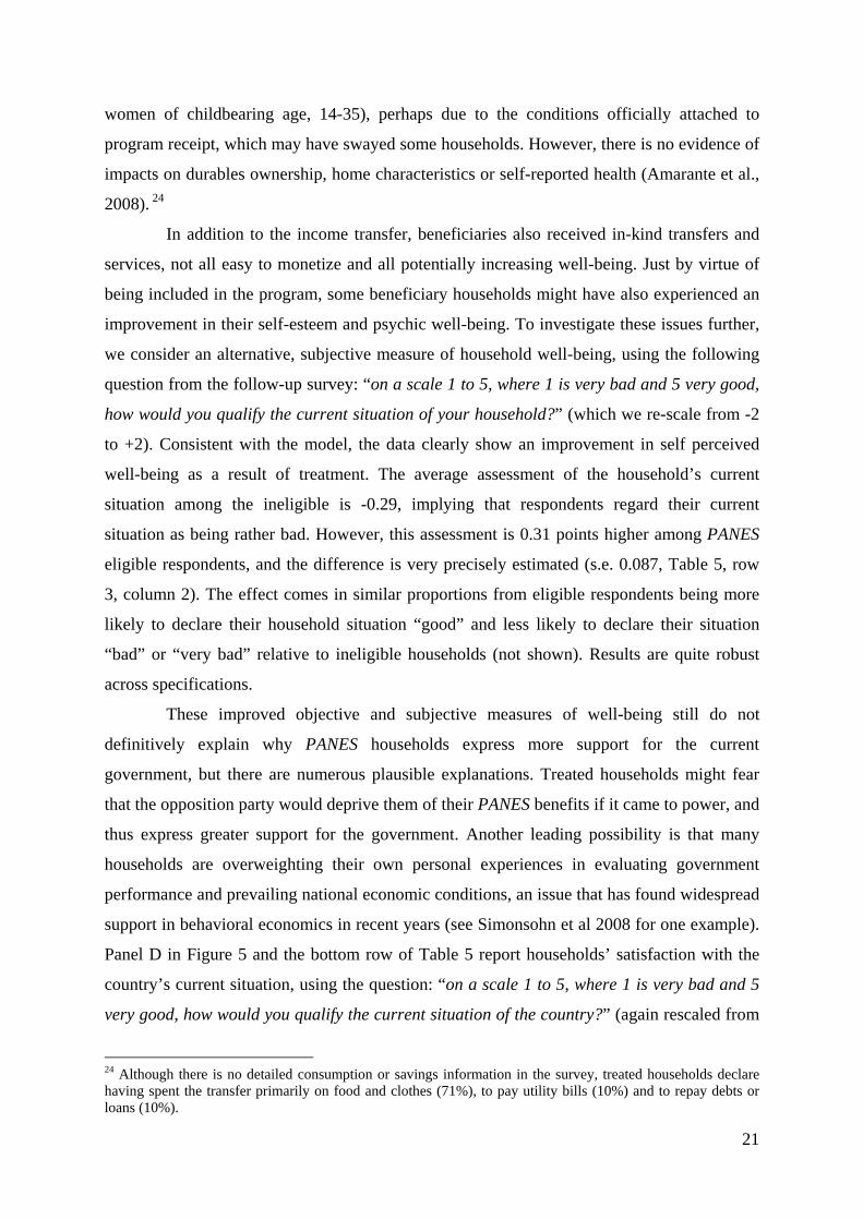
In addition to the income transfer, beneficiaries also received in-kind transfers and

services, not all easy to monetize and all potentially increasing well-being. Just by virtue of

being included in the program, some beneficiary households might have also experienced an

improvement in their self-esteem and psychic well-being. To investigate these issues further,

we consider an alternative, subjective measure of household well-being, using the following

question from the follow-up survey: “on a scale 1 to 5, where 1 is very bad and 5 very good,

how would you qualify the current situation of your household?” (which we re-scale from -2

to +2). Consistent with the model, the data clearly show an improvement in self perceived

well-being as a result of treatment. The average assessment of the household’s current

situation among the ineligible is -0.29, implying that respondents regard their current

situation as being rather bad. However, this assessment is 0.31 points higher among PANES

eligible respondents, and the difference is very precisely estimated (s.e. 0.087, Table 5, row

3, column 2). The effect comes in similar proportions from eligible respondents being more

likely to declare their household situation “good” and less likely to declare their situation

“bad” or “very bad” relative to ineligible households (not shown). Results are quite robust

across specifications.

These improved objective and subjective measures of well-being still do not

definitively explain why PANES households express more support for the current

government, but there are numerous plausible explanations. Treated households might fear

that the opposition party would deprive them of their PANES benefits if it came to power, and

thus express greater support for the government. Another leading possibility is that many

households are overweighting their own personal experiences in evaluating government

performance and prevailing national economic conditions, an issue that has found widespread

support in behavioral economics in recent years (see Simonsohn et al 2008 for one example).

Panel D in Figure 5 and the bottom row of Table 5 report households’ satisfaction with the

country’s current situation, using the question: “on a scale 1 to 5, where 1 is very bad and 5

very good, how would you qualify the current situation of the country?” (again rescaled from

24 Although there is no detailed consumption or savings information in the survey, treated households declare having spent the transfer primarily on food and clothes (71%), to pay utility bills (10%) and to repay debts or loans (10%).

22

-2 to +2). There is limited support for this conjecture: PANES eligible households express a

somewhat more positive assessment of Uruguay’s current situation than the ineligible but the

estimate is not statistically significant in our preferred specification, at 0.097 (s.e. 0.086,

column 2). We present further evidence on channels below in our discussion of the second

follow-up survey round.

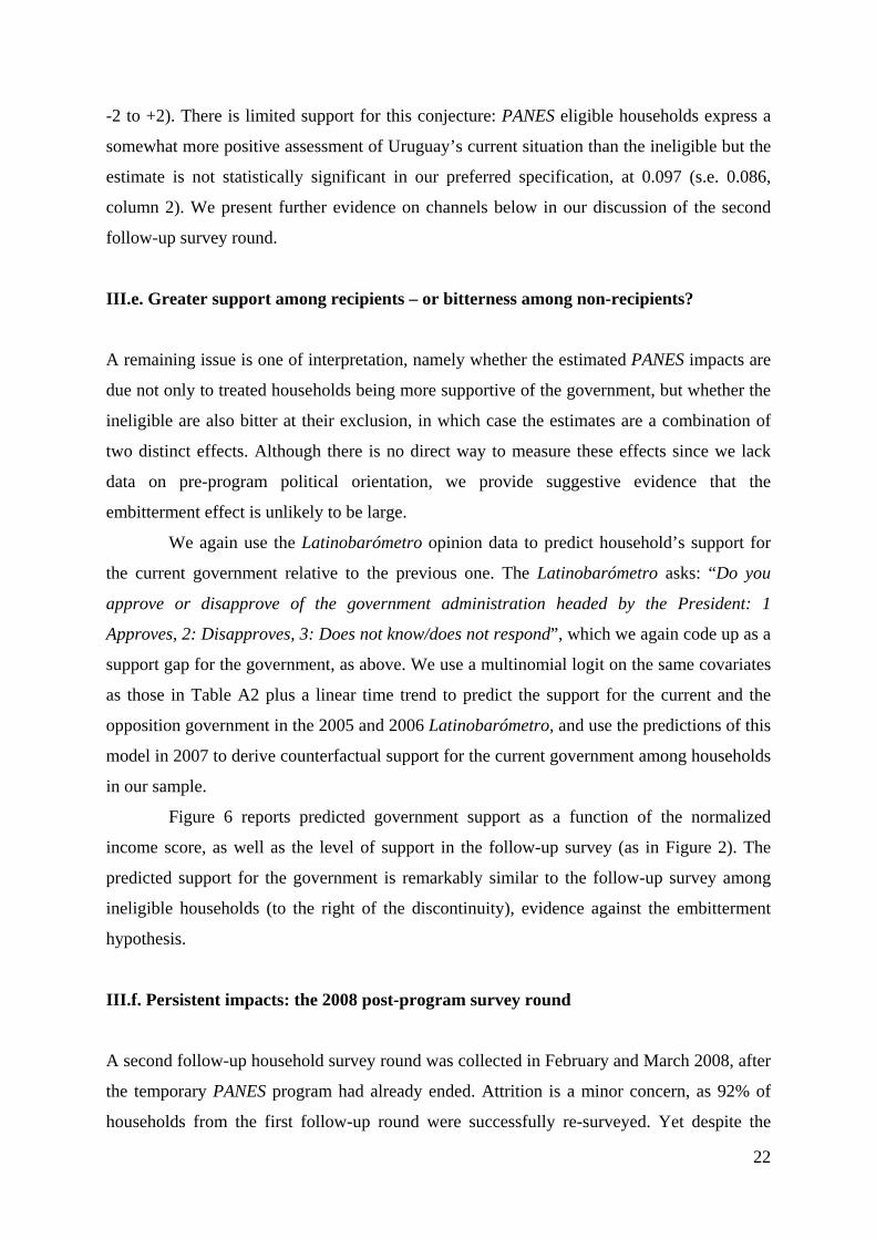
III.e. Greater support among recipients – or bitterness among non-recipients?

A remaining issue is one of interpretation, namely whether the estimated PANES impacts are

due not only to treated households being more supportive of the government, but whether the

ineligible are also bitter at their exclusion, in which case the estimates are a combination of

two distinct effects. Although there is no direct way to measure these effects since we lack

data on pre-program political orientation, we provide suggestive evidence that the

embitterment effect is unlikely to be large.

We again use the Latinobarómetro opinion data to predict household’s support for

the current government relative to the previous one. The Latinobarómetro asks: “Do you

approve or disapprove of the government administration headed by the President: 1

Approves, 2: Disapproves, 3: Does not know/does not respond”, which we again code up as a

support gap for the government, as above. We use a multinomial logit on the same covariates

as those in Table A2 plus a linear time trend to predict the support for the current and the

opposition government in the 2005 and 2006 Latinobarómetro, and use the predictions of this

model in 2007 to derive counterfactual support for the current government among households

in our sample.

Figure 6 reports predicted government support as a function of the normalized

income score, as well as the level of support in the follow-up survey (as in Figure 2). The

predicted support for the government is remarkably similar to the follow-up survey among

ineligible households (to the right of the discontinuity), evidence against the embitterment

hypothesis.

III.f. Persistent impacts: the 2008 post-program survey round

A second follow-up household survey round was collected in February and March 2008, after

the temporary PANES program had already ended. Attrition is a minor concern, as 92% of

households from the first follow-up round were successfully re-surveyed. Yet despite the

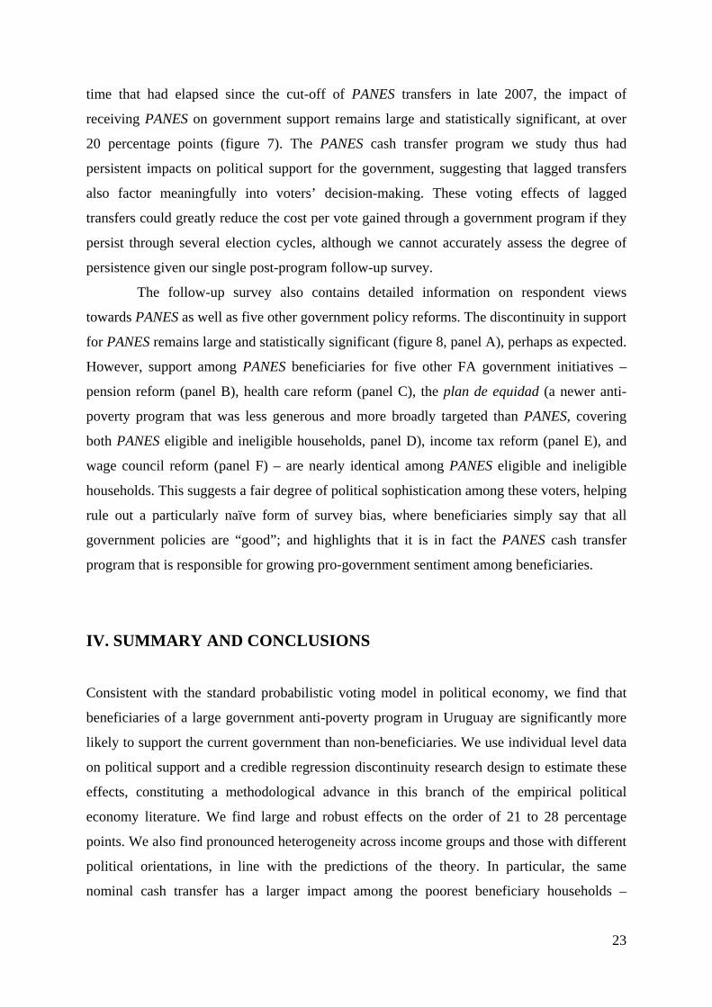
23

time that had elapsed since the cut-off of PANES transfers in late 2007, the impact of

receiving PANES on government support remains large and statistically significant, at over

20 percentage points (figure 7). The PANES cash transfer program we study thus had

persistent impacts on political support for the government, suggesting that lagged transfers

also factor meaningfully into voters’ decision-making. These voting effects of lagged

transfers could greatly reduce the cost per vote gained through a government program if they

persist through several election cycles, although we cannot accurately assess the degree of

persistence given our single post-program follow-up survey.

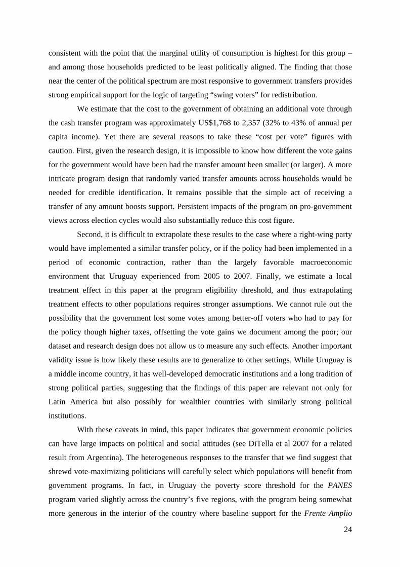
The follow-up survey also contains detailed information on respondent views

towards PANES as well as five other government policy reforms. The discontinuity in support

for PANES remains large and statistically significant (figure 8, panel A), perhaps as expected.

However, support among PANES beneficiaries for five other FA government initiatives –

pension reform (panel B), health care reform (panel C), the plan de equidad (a newer anti-

poverty program that was less generous and more broadly targeted than PANES, covering

both PANES eligible and ineligible households, panel D), income tax reform (panel E), and

wage council reform (panel F) – are nearly identical among PANES eligible and ineligible

households. This suggests a fair degree of political sophistication among these voters, helping

rule out a particularly naïve form of survey bias, where beneficiaries simply say that all

government policies are “good”; and highlights that it is in fact the PANES cash transfer

program that is responsible for growing pro-government sentiment among beneficiaries.

IV. SUMMARY AND CONCLUSIONS

Consistent with the standard probabilistic voting model in political economy, we find that

beneficiaries of a large government anti-poverty program in Uruguay are significantly more

likely to support the current government than non-beneficiaries. We use individual level data

on political support and a credible regression discontinuity research design to estimate these

effects, constituting a methodological advance in this branch of the empirical political

economy literature. We find large and robust effects on the order of 21 to 28 percentage

points. We also find pronounced heterogeneity across income groups and those with different

political orientations, in line with the predictions of the theory. In particular, the same

nominal cash transfer has a larger impact among the poorest beneficiary households –

24

consistent with the point that the marginal utility of consumption is highest for this group –

and among those households predicted to be least politically aligned. The finding that those

near the center of the political spectrum are most responsive to government transfers provides

strong empirical support for the logic of targeting “swing voters” for redistribution.

We estimate that the cost to the government of obtaining an additional vote through

the cash transfer program was approximately US$1,768 to 2,357 (32% to 43% of annual per

capita income). Yet there are several reasons to take these “cost per vote” figures with

caution. First, given the research design, it is impossible to know how different the vote gains

for the government would have been had the transfer amount been smaller (or larger). A more

intricate program design that randomly varied transfer amounts across households would be

needed for credible identification. It remains possible that the simple act of receiving a

transfer of any amount boosts support. Persistent impacts of the program on pro-government

views across election cycles would also substantially reduce this cost figure.

Second, it is difficult to extrapolate these results to the case where a right-wing party

would have implemented a similar transfer policy, or if the policy had been implemented in a

period of economic contraction, rather than the largely favorable macroeconomic

environment that Uruguay experienced from 2005 to 2007. Finally, we estimate a local

treatment effect in this paper at the program eligibility threshold, and thus extrapolating

treatment effects to other populations requires stronger assumptions. We cannot rule out the

possibility that the government lost some votes among better-off voters who had to pay for

the policy though higher taxes, offsetting the vote gains we document among the poor; our

dataset and research design does not allow us to measure any such effects. Another important

validity issue is how likely these results are to generalize to other settings. While Uruguay is

a middle income country, it has well-developed democratic institutions and a long tradition of

strong political parties, suggesting that the findings of this paper are relevant not only for

Latin America but also possibly for wealthier countries with similarly strong political

institutions.

With these caveats in mind, this paper indicates that government economic policies

can have large impacts on political and social attitudes (see DiTella et al 2007 for a related

result from Argentina). The heterogeneous responses to the transfer that we find suggest that

shrewd vote-maximizing politicians will carefully select which populations will benefit from

government programs. In fact, in Uruguay the poverty score threshold for the PANES

program varied slightly across the country’s five regions, with the program being somewhat

more generous in the interior of the country where baseline support for the Frente Amplio

25

government was lower. While we should be cautious about over-interpreting a result based on

only five regions, and have no direct evidence that blatant political considerations directly

entered into the setting of the eligibility thresholds, this pattern is consistent with the

government choosing to deliberately target more program resources to “swing voters” in the

interior and away from their “core supporters” in the capital of Montevideo, a reasonable

political strategy given our findings.

26

Table 1: Human development and democracy in Uruguay and selected countries

UNDP Human Development Report 2007 The Economist Intelligence Unit democracy index Human

Development Index

GDP per

capita (PPP)

Life expectancy

Gross school

enrolment rate

Democracy Rank Electoral process

Functioning of govt.

Political culture

Uruguay 0.852 9,962 75.9 88.9 Full 27 10.00 8.21 6.88 USA 0.951 41,890 77.9 93.3 Full 17 8.75 7.86 8.75 Argentina 0.869 14,280 74.8 89.7 Flawed 54 8.75 5.00 5.63 Brazil 0.800 8,402 71.7 87.5 Flawed 42 9.58 7.86 5.63 Chile 0.867 12,027 78.3 82.9 Flawed 30 9.58 8.93 6.25 Colombia 0.791 7,304 72.3 75.1 Flawed 67 9.17 4.36 4.38 Mexico 0.829 10,751 75.6 75.6 Flawed 53 8.75 6.07 5.00 Venezuela 0.792 6,632 73.2 75.5 Hybrid 93 7.00 3.64 5.00

Source: UNDP (2007) and The Economist Intelligence Unit (2007).

27

Table 2: Program eligibility, participation, and political support for the government

(1) (2) (3) (4) (5) (6) Panel A: First stage: Ever received PANES (dep. var.)

Program eligibility 0.991*** 0.976*** 0.964*** 0.991*** 0.977*** 0.964*** (0.003) (0.010) (0.021) (0.003) (0.010) (0.024) Panel B: Reduced form: Government support (dep. var.)

Program eligibility 0.256*** 0.223*** 0.249*** 0.231*** 0.209*** 0.269*** (0.026) (0.054) (0.087) (0.028) (0.056) (0.090)

Panel C: IV: Government support (dep. var.)

Ever received PANES 0.258*** 0.229*** 0.258*** 0.234*** 0.214*** 0.279*** (0.026) (0.055) (0.089) (0.028) (0.057) (0.093)

Score controls None Linear Quadratic None Linear Quadratic Other controls No No No Yes Yes Yes

Notes: The table reports first stage (Panel A), reduced form (Panel B), and IV (Panel C) estimates of the effect of PANES on political support. The instrument is an indicator for a household score below the eligibility threshold. The endogenous variable is defined as ever having received PANES. Columns 1 to 3 include, in order, a polynomial in the standardized score of degree 0, 1 and 2, and these polynomials interacted with the eligibility indicator. Columns 4 to 6 additionally control for pretreatment characteristics (average household member age, average household education, number of household members, log per-capita income, interview month indicators, age, education and gender of the respondent, departamento indicators). Number of observations in columns 1 to 3: 2,098; in columns 4 to 6: 1,987. Standard errors clustered by score in brackets. Standard errors are almost identical (differing by roughly 1%) when we use the jackknife approach in McCrary (2008b). Statistically significant at 90% (*), 95% (**), and 99% (***) confidence.

28

Table 3: Program eligibility and pre-treatment characteristics, reduced form estimates

Dependent variable: (1) (2) (3) Log per-capita income at baseline -0.046* 0.002 0.011 (0.027) (0.057) (0.093)

Average years of education at baseline 0.056 -0.046 -0.216 (0.101) (0.208) (0.308)

Household size at baseline 0.303*** -0.296 -0.599* (0.116) (0.244) (0.359)

Average age at baseline -3.928*** -0.826 -2.104 (1.087) (2.170) (3.173)

Beneficiary female 0.077*** -0.020 -0.037 (0.029) (0.058) (0.090)

Beneficiary years of education 0.185 0.107 0.279 (0.150) (0.306) (0.445)

Beneficiary age -2.449*** -0.599 -2.138 (0.795) (1.565) (2.363)

Survey non-response rate -0.011 0.047 0.026 (0.018) (0.037) (0.057) Voted in 2004 elections -0.002 0.021 0.037 (0.012) (0.025) (0.044) Score controls None Linear Quadratic

Notes. The table reports results from regressions of various pre-treatment characteristics on the program eligibility indicator. See also notes to Table 2. Number of observations is 2,089, except for survey non-response rate, where it is (3,085).

29

Table 4: Program participation and political support for the government, heterogeneous effects

Panel A: RD estimates by household pre-treatment income

Log pre-treatment household income -0.238*

(0.138)

Panel B: RD estimates by predicted respondent political orientation Predicted likelihood of voting for the opposition 2001-04 3.366**

(1.640)

(Predicted likelihood of voting for the opposition 2001-04) 2 -2.979* (1.560)

Notes. The table reports the estimated effect of program participation on support for the government, as a function of by pre-treatment income (panel A) and by predicted level of support for the opposition coalition (panel B). Regressions performed by GLS with weights equal to the sample size by cell. Number of observations: 30. See text for details.

30

Table 5: Program eligibility and additional outcomes, reduced form estimates

Dependent variable: (1) (2) (3) Per capita income growth 0.221*** 0.251*** 0.188 (0.036) (0.073) (0.120)

Household average weekly hours of work -1.659** 1.811 0.254 (0.754) (1.495) (2.337)

Satisfaction with household situation 0.291*** 0.312*** 0.266** (0.041) (0.087) (0.134) Satisfaction with country situation 0.246*** 0.097 0.043 (0.041) (0.086) (0.138) Score controls None Linear Quadratic Other controls Yes Yes Yes

Notes. The table reports results from regressions of various outcomes on the program eligibility indicator. Regressions include other controls as in columns 4 to 6 of Table 2. See also notes to Table 2.

31

Figure A1. Program eligibility and baseline characteristics Panel A: Log per capita income Panel B: Average years of education Panel C: Household size

5.8

66.

26.

46.

6

-.02 -.01 0 .01 .02Predicted income

3

3.5

44.

55

5.5


22.

53

3.5

44.

5


Panel D: Average age Panel E: Beneficiary female Panel F: Beneficiary years of education

2025

3035

4045


.4.5

.6.7

.8.9


45

67

8


Panel G: Beneficiary age Panel H: Survey non-response

3035

4045

50


.1.2

.3.4

.5


Notes. Panels A to G report the average value of a number of pre-treatment characteristics as a function of the standardized score. Panel H reports survey non-response.

32

. Table A2: Probability of voting for the Frente Amplio: marginal effects

Marginal effect s.e. Female 0.126 (0.128) (Age/10) 0.156*** (0.045) (Age/10) x Female -0.104* (0.060) (Age/10)2 -0.022*** (0.004) (Age/10)2 x Female 0.012** (0.006) Years of education 0.046*** (0.012) Years of education 2 -0.002*** (0.001) Home owner -0.093*** (0.021) Departamento (state) indicators: Artigas -0.334*** (0.055) Cerro Largo -0.096** (0.041) Colonia -0.230*** (0.051) Canelones -0.151*** (0.057) Durazno -0.350*** (0.068) Florida -0.174*** (0.064) Lavalleja -0.339*** (0.058) Maldonado -0.219*** (0.045) Paysandú -0.111** (0.045) Rio Negro -0.428*** (0.044) Rivera -0.236*** (0.060) Rocha -0.261*** (0.068) Salto -0.336*** (0.039) San Jose -0.194*** (0.069) Soriano -0.216*** (0.054) Tacuarembó -0.326*** (0.043) Treinta Y Tres -0.379*** (0.057) Observations 2,909

Notes. The table reports results from a probit model of voting intentions on a number of covariates. The excluded departamento is the capital, Montevideo. Source: Latinobarómetro, 2001-2004.

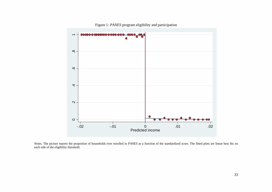
33

Figure 1: PANES program eligibility and participation

0.2

.4.6

.81


Notes. The picture reports the proportion of households ever enrolled in PANES as a function of the standardized score. The fitted plots are linear best fits on each side of the eligibility threshold.

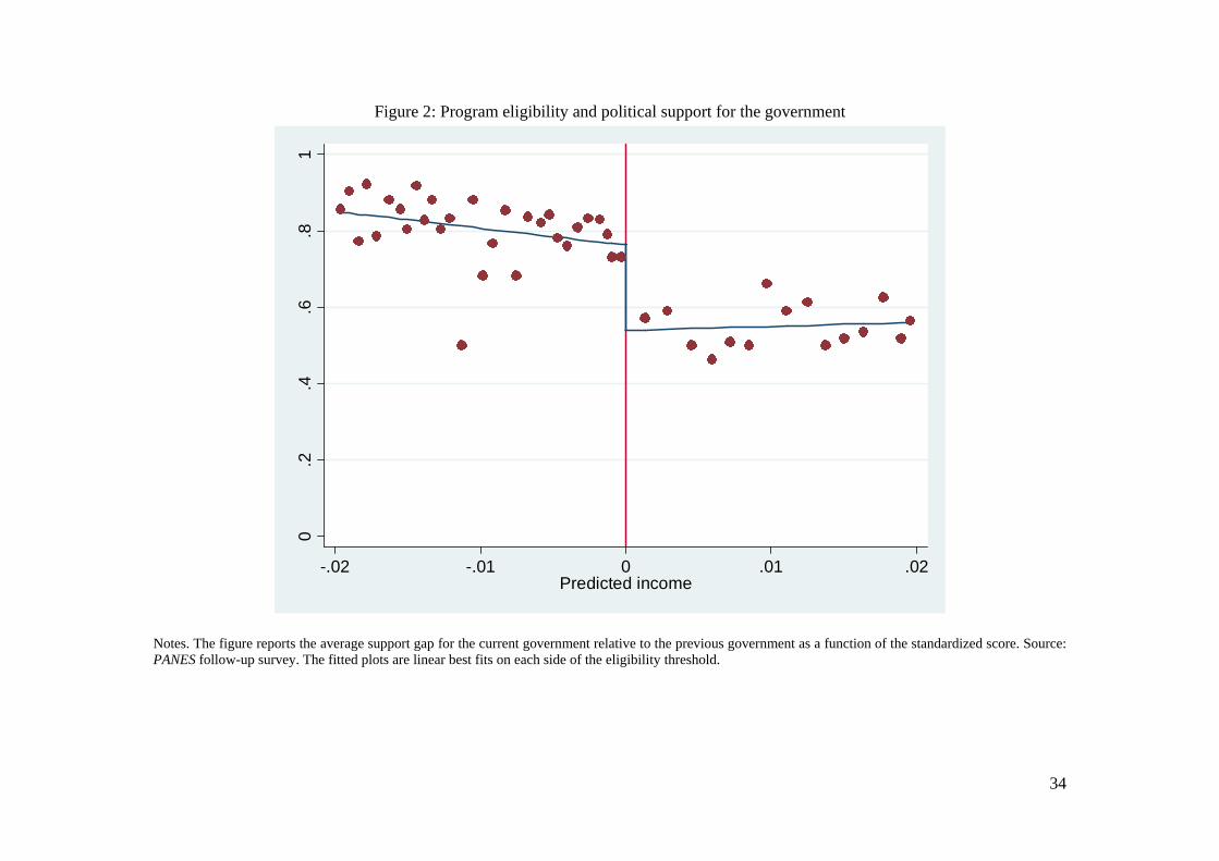
34

Figure 2: Program eligibility and political support for the government

0.2

.4.6

.81


Notes. The figure reports the average support gap for the current government relative to the previous government as a function of the standardized score. Source: PANES follow-up survey. The fitted plots are linear best fits on each side of the eligibility threshold.

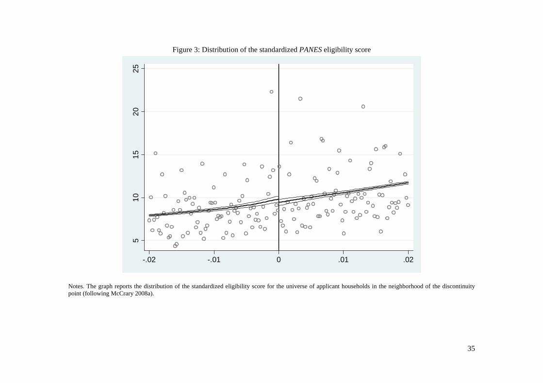
35

Figure 3: Distribution of the standardized PANES eligibility score

510

1520

25

-.02 -.01 0 .01 .02

Notes. The graph reports the distribution of the standardized eligibility score for the universe of applicant households in the neighborhood of the discontinuity point (following McCrary 2008a).

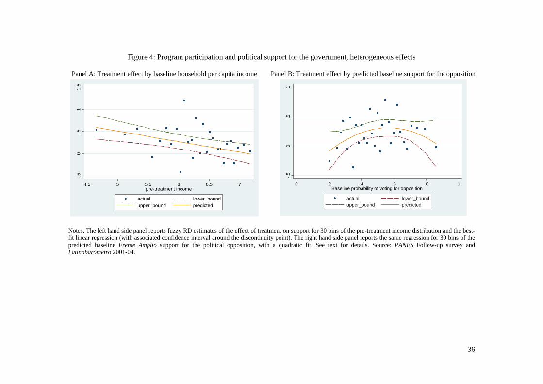
36

Figure 4: Program participation and political support for the government, heterogeneous effects

Panel A: Treatment effect by baseline household per capita income Panel B: Treatment effect by predicted baseline support for the opposition

-.50

.51

1.5

4.5 5 5.5 6 6.5 7pre-treatment income

actual lower_boundupper_bound predicted

-.50

.51

0 .2 .4 .6 .8 1Baseline probability of voting for opposition

actual lower_boundupper_bound predicted

Notes. The left hand side panel reports fuzzy RD estimates of the effect of treatment on support for 30 bins of the pre-treatment income distribution and the best-fit linear regression (with associated confidence interval around the discontinuity point). The right hand side panel reports the same regression for 30 bins of the predicted baseline Frente Amplio support for the political opposition, with a quadratic fit. See text for details. Source: PANES Follow-up survey and Latinobarómetro 2001-04.

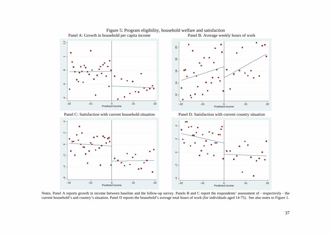
37

Figure 5: Program eligibility, household welfare and satisfaction Panel A: Growth in household per capita income Panel B: Average weekly hours of work

.4.6

.81

1.2


1214

1618

20


Panel C: Satisfaction with current household situation Panel D: Satisfaction with current country situation

-.6-.4

-.20

.2.4


-.4-.2

0.2

.4


Notes. Panel A reports growth in income between baseline and the follow-up survey. Panels B and C report the respondents’ assessment of - respectively - the current household’s and country’s situation. Panel D reports the household’s average total hours of work (for individuals aged 14-75). See also notes to Figure 1.

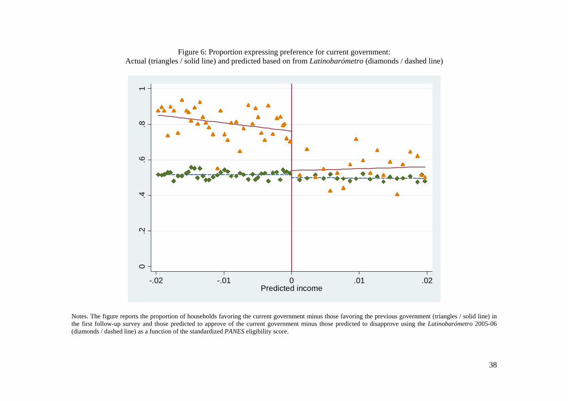
38

Figure 6: Proportion expressing preference for current government: Actual (triangles / solid line) and predicted based on from Latinobarómetro (diamonds / dashed line)

0.2

.4.6

.81


Notes. The figure reports the proportion of households favoring the current government minus those favoring the previous government (triangles / solid line) in the first follow-up survey and those predicted to approve of the current government minus those predicted to disapprove using the Latinobarómetro 2005-06 (diamonds / dashed line) as a function of the standardized PANES eligibility score.

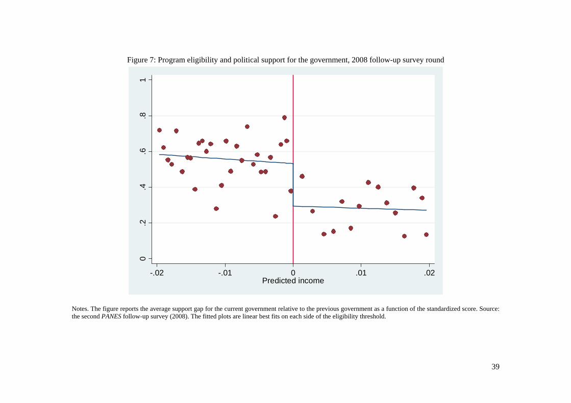
39

Figure 7: Program eligibility and political support for the government, 2008 follow-up survey round

0.2

.4.6

.81


Notes. The figure reports the average support gap for the current government relative to the previous government as a function of the standardized score. Source: the second PANES follow-up survey (2008). The fitted plots are linear best fits on each side of the eligibility threshold.

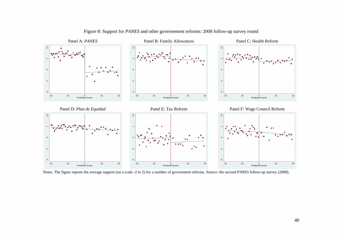
40

Figure 8: Support for PANES and other governement reforms: 2008 follow-up survey round

Panel A: PANES Panel B: Family Allowances Panel C: Health Reform -.5

0.5

11.

5


-.50

.51

1.5


-.50

.51

1.5


Panel D: Plan de Equidad Panel E: Tax Reform Panel F: Wage Council Reform

-.50

.51

1.5


-.50

.51

1.5


-.50

.51

1.5


Notes. The figure reports the average support (on a scale -2 to 2) for a number of government reforms. Source: the second PANES follow-up survey (2008).

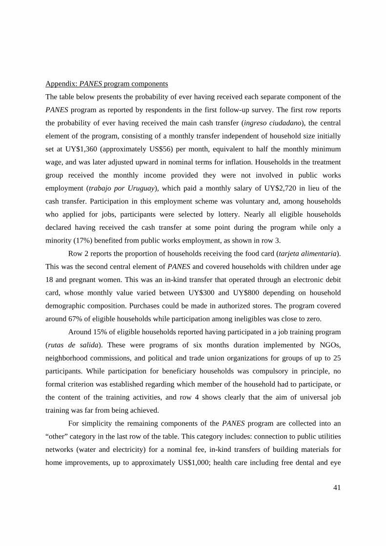
41

Appendix: PANES program components

The table below presents the probability of ever having received each separate component of the

PANES program as reported by respondents in the first follow-up survey. The first row reports

the probability of ever having received the main cash transfer (ingreso ciudadano), the central

element of the program, consisting of a monthly transfer independent of household size initially

set at UY$1,360 (approximately US$56) per month, equivalent to half the monthly minimum

wage, and was later adjusted upward in nominal terms for inflation. Households in the treatment

group received the monthly income provided they were not involved in public works

employment (trabajo por Uruguay), which paid a monthly salary of UY$2,720 in lieu of the

cash transfer. Participation in this employment scheme was voluntary and, among households

who applied for jobs, participants were selected by lottery. Nearly all eligible households

declared having received the cash transfer at some point during the program while only a

minority (17%) benefited from public works employment, as shown in row 3.

Row 2 reports the proportion of households receiving the food card (tarjeta alimentaria).

This was the second central element of PANES and covered households with children under age

18 and pregnant women. This was an in-kind transfer that operated through an electronic debit

card, whose monthly value varied between UY$300 and UY$800 depending on household

demographic composition. Purchases could be made in authorized stores. The program covered

around 67% of eligible households while participation among ineligibles was close to zero.

Around 15% of eligible households reported having participated in a job training program

(rutas de salida). These were programs of six months duration implemented by NGOs,

neighborhood commissions, and political and trade union organizations for groups of up to 25

participants. While participation for beneficiary households was compulsory in principle, no

formal criterion was established regarding which member of the household had to participate, or

the content of the training activities, and row 4 shows clearly that the aim of universal job

training was far from being achieved.

For simplicity the remaining components of the PANES program are collected into an

“other” category in the last row of the table. This category includes: connection to public utilities

networks (water and electricity) for a nominal fee, in-kind transfers of building materials for

home improvements, up to approximately US$1,000; health care including free dental and eye

42

care (e.g., cataract surgery performed in Cuba) and prostheses; micro-finance loans and technical

assistance for small entrepreneurial activities; and temporary accommodation for homeless

households. Overall, around 21% of beneficiary households reported having received at least one

of these additional components. Additional government programs that affected both PANES

beneficiary and non-beneficiary households included additional school teachers in disadvantaged

neighborhoods (maestros comunitarios) and improved access to the public health sector.

Appendix Table A1: Self-reported PANES take-up among beneficiaries, by component (%)

Citizen Income 97.6

Food card 66.9

Public works employment 17.0

Job training 15.1

Other components 21.3

43

REFERENCES Adato M., B. de la Brière, D. Mindek and A. Quisumbing (2000), The Impact of Progresa on

Women’s Status and Intrahousehold Relations, Final Report, International Food Policy Research Institute, Washington D.C.

Arim R., Amarante V. and Vigorito A. (2005), “Criterios para la selección de beneficiarios del Plan de Atención Nacional a la Emergencia Social”, mimeo, Universidad de la Republica, Instituto de Economía, Montevideo.

Amarante V., G. Burdín, M. Manacorda and A. Vigorito (2008), “Informe final de la evaluación intermedia del impacto del PANES”, mimeo, Universidad de la Republica, Instituto de Economía, Montevideo.

Card D., R. Chetty, and A. Weber (2007). “Cash-on-Hand and Competing Models of Intertemporal Behavior: New Evidence from the Labor Market”, Quarterly Journal of Economics, 122(4): 1511-1560.

Card D. and D. Lee (2008), “Regression discontinuity inference with specification error”, Journal of Econometrics, 142, (2), (February 2008), 655-674.

Case A. (2001), “Election goals and income redistribution: Recent evidence from Albania”, European Economic Review, 45 (2001), 405-423.

Chen, Jowei (2008a), “When do government benefits influence voters’ behavior? The effect of FEMA disaster awards on US Presidential votes”, mimeo., Stanford University.

Chen, Jowei (2008b), “Are poor voters easier to buy off? A natural experiment from the 2004 Florida hurricane season”, mimeo., Stanford University.

Conover E. and A. Camacho (2007), “Manipulation of Social Program Eligibility: Detection, Explanations and Consequences for Empirical Research” mimeo, U.C. Berkeley.

Cox G.W. and D. McCubbins (1986), “Electoral Politics as a Redistributive Game”, Journal of Politics, 48(May), 370-389.

Dahlberg M. and E. Eva Johansson (2002), “On the Vote-Purchasing Behavior of Incumbent Governments”, American Political Science Review, Vol. 96, No. 1. (Mar., 2002), 27-40.

DiNardo J. and D. Lee (2004), “Economic Impacts of New Unionization on Private Sector Employers: 1984-2001”, Quarterly Journal of Economics, 119(4), 1383-1441.

DiTella, R., S. Galiani, and E. Schargrodsky (2007). “The Formation of Beliefs: Evidence from the Allocation of Land Titles to Squatters”, Quarterly Journal of Economics, 122 (1), 209-241.

Dixit A. and J. Londregan (1996), “The Determinants of Success of Special Interests in Redistributive Politics”, Journal of Politics, Vol. 58, No. 4. (Nov., 1996), 1132-1155.

Dixit A. and J. Londregan (1998), “Ideology, Tactics, and Efficiency in Redistributive Politics”, Quarterly Journal of Economics, 113(2), 497-529.

The Economist Intelligence Unit (2007), The World in 2007, London. Green T. (2006a), “Do Social Transfer Programs Affect Voter Behavior? Evidence from

PROGRESA in Mexico, 1997-2000”, mimeo, U.C., Berkeley. Green T. (2006b), “The Political Economy of a Social Transfer Program: Evidence on the

Distribution of PROGRESA in Mexico, 1997-2000”, mimeo, U,C., Berkeley. Lemieux T. and K. Milligan (2008), “Incentive effects of social assistance: A regression

discontinuity approach”, Journal of Econometrics, 142, (2), (February 2008), 807-828. Levitt S.D. and J.M. Snyder (1997), “The Impact of Federal Spending on House Election

Outcomes”, Journal of Political Economy, Vol. 105, No. 1. (Feb., 1997), 30-53.

44

Lindbek A. and H.W. Weibull (1987), “Balanced-budget redistribution as the outcome of political competition, Public Choice, 52, 273-297.

Markus G. B (1988),"The Impact of Personal and National Economic Conditions on the Presidential Vote: A Pooled Cross-Sectional Analysis”, American Journal of Political Science, 32, No. 1. (Feb., 1988), 137-15.

McCrary J., (2008a). “Manipulation of the running variable in the regression discontinuity design: A density test”, Journal of Econometrics, 142, (2), (February 2008), 698-714.

McCrary J. (2008b). “Inference and Specification Testing in the Regression Discontinuity Design”, mimeo., U.C. Berkeley.

Parker S.W. and E. Skoufias (2000), The Impact of Progresa on Work, Leisure, and Time Allocation, Final Report, International Food Policy Research Institute, Washington D.C.

Persson T. and G. Tabellini (2002), Political Economics: Explaining Economic Policy, MIT Press: Cambridge MA.

Rawlings, L., and G. Rubio (2005), “Evaluating the Impact of Conditional Cash Transfer Programs.” World Bank Research Observer 20(1):29–55.

Schady N.R. (2000), “The Political Economy of Expenditures by the Peruvian Social Fund (FONCODES), 1991-95”, American Political Science Review, 94, No. 2 June 2000.

Schaffer, F. C. (2007), “Lessons learned? (Chapter 11)”, in F. C. Schaffer, ed., Elections for Sale: The Causes and Consequences of Vote Buying, Boulder, CO: Lynne Rienner.

Simonsohn, U., Karlsson, N., Loewenstein, G. and Ariely, D. (2008) “The Tree of Experience in the Forest of Information: Overweighing Experienced Relative to Observed Information” Games and Economic Behavior, 62, pp. 263-286

Sole-Olle, A. and P. Sorribas-Navarro. (2008), “Does Partisan Alignment Affect the Electoral Reward of Intergovernmental Transfers?” CESifo Working Paper, No. 2335.

Stokes, S. C. (2005), “Perverse accountability: A formal model of machine politics with evidence from Argentina”, American Political Science Review, 99(3), 315-325.

UNDP (2007), Human Development Report 2007/2008: Fighting climate change: Human solidarity in a divided world, New-York.

UNDP (2008), Política, políticas y desarrollo humano. Informe Nacional de Desarrollo Humano, Montevideo.

Verdier T. and J.M. Snyder (2002), “The Political Economy of Clientelism”, CEPR discussion papers, 3205.

CENTRE FOR ECONOMIC PERFORMANCE Recent Discussion Papers

911 Philippe Aghion John Van Reenen Luigi Zingales

Innovation and Institutional Ownership

910 Fabian Waldinger Peer Effects in Science – Evidence from the Dismissal of Scientists in Nazi Germany

909 Tomer Blumkin Yossi Hadar Eran Yashiv

The Macroeconomic Role of Unemployment Compensation

908 Natalie Chen Dennis Novy

International Trade Integration: A Disaggregated Approach

907 Dongshu Ou To Leave or Not to Leave? A Regression Discontinuity Analysis of the Impact of Failing the High School Exit Exam

906 Andrew B. Bernard J. Bradford Jensen Stephen J. Redding Peter K. Schott

The Margins of US Trade

905 Gianluca Benigno Bianca De Paoli

On the International Dimension of Fiscal Policy

904 Stephen J. Redding Economic Geography: A Review of the Theoretical and Empirical Literature

903 Andreas Georgiadis Alan Manning

Change and Continuity Among Minority Communities in Britain

902 Maria Bas Trade, Technology Adoption and Wage Inequalities: Theory and Evidence

901 Holger Breinlich Chiara Criscuolo

Service Traders in the UK

900 Emanuel Ornelas John L. Turner

Protection and International Sourcing

899 Kosuke Aoki Takeshi Kimura

Central Bank's Two-Way Communication with the Public and Inflation Dynamics

898 Alan Manning Farzad Saidi

Understanding the Gender Pay Gap: What’s Competition Got to Do with It?

897 David M. Clark Richard Layard Rachel Smithies

Improving Access to Psychological Therapy: Initial Evaluation of the Two Demonstration Sites

896 Giorgio Barba Navaretti Riccardo Faini Alessandra Tucci

Does Family Control Affect Trade Performance? Evidence for Italian Firms

895 Jang Ping Thia Why Capital Does Not Migrate to the South: A New Economic Geography Perspective

894 Kristian Behrens Frédéric Robert-Nicoud

Survival of the Fittest in Cities: Agglomeration, Selection and Polarisation

893 Sharon Belenzon Mark Schankerman

Motivation and Sorting in Open Source Software Innovation

892 Guy Michaels Ferdinand Rauch Stephen J. Redding

Urbanization and Structural Transformation

891 Nicholas Bloom Christos Genakos Ralf Martin Raffaella Sadun

Modern Management: Good for the Environment or Just Hot Air?

890 Paul Dolan Robert Metcalfe

Comparing willingness-to-pay and subjective well- being in the context of non-market goods

889 Alberto Galasso Mark Schankerman

Patent Thickets and the Market for Innovation: Evidence from Settlement of Patent Disputes

888 Raffaella Sadun Does Planning Regulation Protect Independent Retailers?

887 Bernardo Guimaraes Kevin Sheedy

Sales and Monetary Policy

886 Andrew E. Clark David Masclet Marie-Claire Villeval

Effort and Comparison Income Experimental and Survey Evidence

885 Alex Bryson Richard B. Freeman

How Does Shared Capitalism Affect Economic Performance in the UK?

884 Paul Willman Rafael Gomez Alex Bryson

Trading Places: Employers, Unions and the Manufacture of Voice

883 Jang Ping Thia The Impact of Trade on Aggregate Productivity and Welfare with Heterogeneous Firms and Business Cycle Uncertainty

882 Richard B. Freeman When Workers Share in Profits: Effort and Responses to Shirking

The Centre for Economic Performance Publications Unit Tel 020 7955 7284 Fax 020 7955 7595 Email [email protected]

Web site http://cep.lse.ac.uk

Documents

CEP Discussion Paper No 912 March 2009 Government ...eprints.lse.ac.uk/28519/1/dp0912.pdf · Sole-Olle and Sorribas-Navarro (2008) use the same approach as Levitt and Snyder (1997)