CFD ANALYSIS OF SCREW COMPRESSOR PERFORMANCE

Ahmed Kovacevic, Nikola Stosic and Ian K. Smith

Centre for Positive Displacement Compressor Technology,

City University, London EC1V OHB, U.K. e-mail: a.kovacevic@city.ac.uk

ABSTRACT Modern manufacturing methods enable screw compressors to be constructed to such close tolerances that full 3-D numerical calculation of the heat and fluid flow through them is required to obtain the maximum possible improvements in their design. An independent stand-alone CAD-CFD interface program has therefore been developed by the authors in order to generate a numerical grid for this purpose. Modifications implemented to the CFD procedure improved solutions in complex domains with strong pressure gradients. The interface employs a rack-generation procedure to produce rotor profiles and an analytical transfinite interpolation method to obtain a fully structured 3-D numerical mesh, which is directly transferable to a CFD code. Some additional features, which include an adaptive meshing procedure, mesh orthogonalization and smoothing, are employed to generate a numerical mesh which can take advantage of the techniques used in recent finite volume numerical method solvers. These were required to overcome problems associated with

i) rotor domains which stretch and slide relative to each other and along the housing ii) robust calculations in domains with significantly different geometry ranges. iii) a grid moving technique with a constant number of vertices.

Some changes had to be made within the solver to increase the speed of calculation. These include a means to maintain constant pressures at the inlet and outlet ports and consideration of two phase flow resulting from oil injection in the working chamber. The pre-processor code and calculating method have been tested on a commercial CFD solver to obtain flow simulations and integral parameter calculations. The results of calculations on an oil injected screw compressor are presented in this paper and compared with experimental results. Good agreement was obtained between them. 1. INTRODUCTION Approximately 17% of all electrical power generated is used to drive compressors while about 80% of all such machines currently manufactured for industrial applications are of the screw type. Improvements in the efficiency of screw compressors can therefore lead to significant energy savings at global level.

The design parameter which influences screw compressor performance most strongly is the rotor profile and differences in shape, which can hardly be detected by eye can effect significant changes in flow rates delivered and power consumption. Other features of the design also strongly affect the overall compressor performance. Thus, clearances between the rotors and between the rotors and the casing determine the leakage through the compressor and hence both the volume flow rate and the power consumption. The shape and position of the suction and discharge ports influence the dynamic losses and, in the case of oil injected machines, the oil injection port position and the quantity of oil injected into the working chamber affect both the outlet temperature and the power consumption. Dimensionless or quasi-steady mathematical models predict the overall effects of changes in these parameters on compressor overall behaviour fairly accurately. However, how the internal flow within the machine is affected locally by changes in these parameters is only approximated by such models. Consequently, the simplified analytical models currently in use are not sufficiently accurate to design screw compressors to obtain the maximum possible improvements from the close manufacturing tolerances now achievable with contemporary numerically controlled machine tools. It is therefore timely to apply a more complex analytical procedure, such as a 3-D Computational Fluid Dynamics (CFD) method to determine the effects of changes in the compressor geometry on internal heat and fluid flow. Such an approach can produce reliable predictions only if calculated over a substantial number of grid points. Hence, a high computer potential and capacity is needed in order to use such procedures to analyse a screw compressor. If an inadequate numerical grid is used, or the solver parameters are not selected carefully, a convergent numerical solution may not be obtained. Calculation results must therefore be monitored closely and compared with the experimental data in order to avoid obtaining results which do not accord with real flow conditions. There is a current trend in CFD methods to improve the accuracy and reliability of numerical simulation without a significant increase in the number of computational points and operations. This may be a significant factor in enabling such methods to be used as an aid to compressor design. Apart from the authors' publications [5]-[7], and [16], there is hardly any reported activity in the use of CFD for screw compressor studies. This is mainly because the existing grid generators and the majority of solvers are still too weak to cope with the problems associated with both the screw compressor geometry and physics of the compression process. Since a screw compressor comprises both moving rotors and a stationary housing, any numerical grid applied must move, slide and deform. Moreover, if flow is to be calculated through the compressor clearances, the geometric length scale ratio of the working chamber may rise to 1000:1. This cannot be done with the majority of existing CFD grid generators. Despite this, the grid aspect ratio should be kept very low. Compressor flow, even in its simplest form, is further complicated by sharp pressure changes and high accelerations, which may drastically affect the flow structure. If, in addition, the working fluid is a real gas or a two-phase fluid or it contains particles, then there are hardly any CFD solver capable to produce a straightforward solution. Therefore, special care is needed to blend the grid generation procedure with an adequate numerical solver to obtain a useful numerical solution of screw compressor processes. Demirdzic and Peric, [1], [2] and Peric [11] set the guidelines for successful finite volume calculation of 3-D flows in complex curvilinear geometries. Based on this, Ferziger and Peric [4] published a book on finite volume methods for fluid dynamics. Muzaferija [10] applied unstructured grids and used a multigrid method to accelerate calculations. Demirdzic and Muzaferija [3] showed the possibility of simultaneous application of the same numerical methods in fluid flow and structural analysis within moving frames. Contemporary grid generation methods are extensively discussed by many authors. The most detailed textbooks are Liseikin [9] and Thompson et al [18]. Adequately applied, the grid generation they describe, accompanied by an appropriate CFD solver, can lead to the successful prediction of screw compressor thermo-fluid flow. Such an approach resulted in the algebraic grid generation method, which employs a multi parameter one-dimensional adaptation. This is given in detail by the authors in [6] and [7], where an interface, which transfers the screw

compressor geometry to a CFD solver, is also described and compressor suction flow is given as a working example. An advanced grid generation procedure is described in this paper. By its use and the inclusion of additional source terms and boundary conditions in the standard governing equations, heat and fluid flow within a screw compressor can be estimated by use of existing CFD solvers. Once the velocity and pressure distribution are determined within the compressor, overall performance parameters such as flow rate, rotor loads, torque and power input may be derived from them. Consequently, the more conventional performance criteria used by compressor manufacturers, such as specific power and volumetric and adiabatic efficiencies can be calculated. These derived values may also be used for comparison of compressors and for further applications like rotor and compressor minimization and optimisation.

2 GENERATION OF A SCREW COMPRESSOR GRID

2.1 Fundamentals An appropriate numerical grid must be generated as a necessary preliminary to a CFD calculation. The grid must define both the stationary and moving parts of the compressor. The rotors form the most complex part of the screw compressor grid and are the most important components since it is within the rotor interlobe chambers that the compression process occurs. Depending on the relative position of the rotors and the housing, the processes of suction, compression and discharge will occur within the compressor. Rotor rotation results in change in the volume of the chambers, which increases the pressure, while internal pressure changes cause leakage flow between the chambers. To apply a CFD procedure, the compressor spatial domain must be replaced by a grid which contains discrete volumes. The number of these volumes depends on the problem dimensionality and accuracy required. A composite grid, made of several structured grids patched together and based on a single boundary fitted co-ordinate system is used to transform the compressor geometry into discrete volumes. Grids are then connected over defined regions on their boundaries which coincide with other parts of the entire numerical mesh. More details of the different grid types and the relative advantages of each grid system are given by Shih et al [12]. The grid generation for compressor rotors starts with the definition of their spatial domains determined by the rotor profile coordinates and their derivatives. These are obtained by means of the rack generation procedure described in detail by Stosic [17]. The grid components define all connections between the rotors and the housing and contain the interlobe, tip and blow-hole leakage paths. The mesh calculation is based on an algebraic transfinite interpolation procedure with a static multi parameter adaptation. This includes stretching functions to ensure grid orthogonality and smoothness. More information about this particular grid generation method can be found in [5]. A grid for the stationary compressor components, like the housing and ports, is also produced. The suction port is divided into five sub-domains, while the discharge chamber consists of three sub-domains. The complete grid generation procedure is programmed in FORTRAN and ensures automatic grid formation for various compressor shapes and sizes, given the housing geometry parameters.

2.2 Discretization of the screw compressor rotor boundaries In general, the number of points required to define the rotor geometry accurately is not large. However, the number needed to establish a sliding interface between them may be so large that the numerical mesh, so formed cannot be solved. One means of resolving this problem, which combines accuracy with fast solution, is to keep the number of computational cells as low as possible and to

modify the distribution of points according to local requirements. An additional reason for such an approach is the large aspect ratio of the screw compressor chamber, the dimensions of which vary from several micrometers to tens of millimetres. In case of the numerical mesh for the compressor presented in this paper, the grid length scale ratio is about 300. Since the number of cells in the radial direction is the same in the chamber as in the gaps, the ratio between the circumferential and radial dimensions of the cell becomes unacceptable. However, the same number of cells can form a convenient grid if the grid adaptation is carefully applied to keep the grid aspect ratio as uniform as possible. The majority of grid generation methods produce numerical grids by use of just one adaptation variable. However, within a complex geometry, various parameters determine the distribution of numerical points. For example, in the case of long narrow clearances, the distance between the points should be smaller. Similarly, a shorter distance between the points is needed in regions where the curvature is high. Also, the point distribution in the rotor contact area should be modified to fulfil requirements of a block connection procedure in the CFD code. In such cases, adaptation by means of two or more variables or conditions is necessary. The different adaptation criteria, like the radius of curvature, distance from the rotor centre or angle of the tangent are applied independently in the static adaptation procedure, developed by authors, to ensure a viable numerical grid. In the example given, two adaptation functions are used simultaneously. The tangent angle and a radius of curvature are applied to the male rotor. For the female rotor the flatness of the curve and the point centre distance are used as criteria for adaptation

2.3 Transfinite interpolation To generate a three-dimensional numerical mesh of a screw compressor, the domain was divided into a number of cross sections along the rotor axis (Fig 4). Each cross section was then calculated separately as a 2D face for both rotors by means of the following steps:

1) Transformation from the ‘physical’ domain to the numerical non-dimensional domain. 2) Definition of the edges by applying an adaptive technique, 3) Selection and matching of four non-contacting boundaries. 4) Calculation of the curves, which connect the facing boundaries by transfinite interpolation. 5) Application of a stretching function to obtain the distribution of the grid points. 6) Orthogonalization, smoothing and final checking of the grid consistency.

Once the boundary faces are produced in steps 1-3, the distribution of internal points in steps 4-6 can be found. A good summary of how to find the internal points from the boundary data by analytical transfinite interpolation is given by Smith [13]. The coordinates of the two opposite boundaries expressed in vector form are:

1

1

( , ) ( , ), 1,2

( , ) ( , ), 1 ,2 ,

l

l

a r l

b r l

ξ η ξ η

ξ η ξ η

= =

= =

r rr r (1)

where the coordinates of the transformed computational coordinate system,ξ and η , are: ( 1)/( 1)i Iξ = − − and ( 1)/( 1)j Jη = − − . i and j denote point numbers on the physical coordinate while I and J are overal number of points on this coordinates. The interior point then can be calculated as:

2

1 11

2

1 1 1 11

( , ) ( ) ( )

( , ) ( , ) ( )[ ( ) ( , )] ,

ll

ll

r a

r r b r

ξ η α ξ η

ξ η ξ η β η ξ ξ η

=

=

=

= + −

∑

∑

r r

rr r r (2)

The blending functions 1 ( )α ξ and 1( )β η can be arbitrary but must satisfy the cardinality conditions, given by (3), to ensure that the edges are reproduced as a part of the solution.

1

1

( ) , =1,2 =1,2

( ) , =1,2 =1,2k kl

k kl

k l

k l

α ξ δ

β η δ

==

(3)

δ is Kronecker’s delta function. By use of equation (3), equation (2) for the 2-D domain can be written in the following general form, which connects the physical and numerical domain coordinates:

1 1 2 2

1 1 2 2

( , ) ( , ) ( ) ( , ) ( )

( , ) ( , ) ( ) ( , ) ( )

x X X

y Y Y

ξ η ξ η α ξ ξ η α ξ

ξ η ξ η β η ξ η β η

= += +

(4)

The success of the analytical transfinite interpolation method (4) to produce regular distribution of the internal points is highly dependent on the selection of blending functions. The simplest method to obtain the blending functions is Langrangian interpolation. However, it produces a satisfactory mesh only for simple problems and this is not case of the screw compressor. A better and more accurate solution can be obtained by Hermite interpolation. More details of Hermite interpolation are given by Smith, [13], Shih et al [12], and Thomson et al [18]. Only the final form of the equations is presented here. The four-boundary method, which assumes interpolation between all four boundaries of the 2-D domain can be written in the following form:

( , ) '( , ) ( , )

( , ) '( , ) ( , )

x x x

y y y

ξ η ξ η ξ η

ξ η ξ η ξ η

= + ∆= + ∆

(5)

If the second term in equation (5) is neglected, then the first term on the right side of the equation implements the two-boundary method, which interpolates between two non connecting boundaries:

1 1 2 2 3 4

1 1 2 2 3 4

( , 0) ( , 1)'( , ) ( ) ( ) ( ) ( ) ( ) ( )

( , 0) ( , 1)'( , ) ( ) ( ) ( ) ( ) ( ) ( )

x xx X h X h h h

y yy Y h Y h h h

ξ η ξ ηξ η ξ η ξ η η ηη η

ξ η ξ ηξ η ξ η ξ η η ηη η

∂ = ∂ == + + +∂ ∂

∂ = ∂ == + + +∂ ∂

(6)

where h1, h2, h3 and h4 are the Hermite interpolation blending functions given as:

3 2 3 21 2

3 2 3 23 1

2 3 1, 2 3

2 ,

h h

h h

η η η η

η η η η η

= − + = − +

= − + = − (7)

The boundary points are defined as:

1 1 1 1

2 2 2 2

( , 0) ( ), ( , 0) ( )

( , 1) ( ), ( , 1) ( )

X x X Y y Y

X x X Y y Y

ξ η ξ ξ η ξ

ξ η ξ ξ η ξ

= = = = = == = = = = =

(8)

The aim of the partial derivatives at the boundaries is to ensure orthogonality. These are:

1 21 2

1 21 2

( , 0) ( , 1)( )( ) ( )( )

( , 0) ( , 1)( )( ) ( )( )

Y Yx xK K

X Xy yK K

ξ η ξ ηξ ξη ξ η ξ

ξ η ξ ηξ ξη ξ η ξ

∂ ∂∂ = ∂ == − = −∂ ∂ ∂ ∂

∂ ∂∂ = ∂ == − − = − −∂ ∂ ∂ ∂

(9)

The coefficients K1 and K2 are positive numbers smalle r than 1. They are usually chosen by trial and error to avoid overlapping of connecting curves inside the domain. For the four-boundaries method, only two additional boundaries have to be mapped. They are:

3 3 3 3

4 4 4 4

( 0, ) ( ) ( 0, ) ( )

( 1, ) ( ) ( 1, ) ( )

X x X Y y Y

X x X Y y Y

ξ η η ξ η η

ξ η η ξ η η

= = = = = == = = = = =

(10)

If the second term in equation (5) is not neglected , itdefines the mapping between the other two boundaries:

3 3 5 4 4 6 7

8

3 3 5 4 4 6 7

( 0, ) '( 0, )( , ) ( ' ) ( ) ( ' ) ( ) ( )

( 1, ) '( 1, )( )

( 0, ) '( 0, )( , ) ( ' ) ( ) ( ' ) ( ) ( )

( 1, ) '( 1,

x xx X X h X X h h

x xh

y yy Y Y h Y Y h h

y y

ξ η ξ ηξ η ξ ξ ξξ ξ

ξ η ξ ηξ

ξ ξ

ξ η ξ ηξ η ξ ξ ξξ ξ

ξ η ξ ηξ

∂ = ∂ =∆ = − + − + − ∂ ∂ ∂ = ∂ =

+ − ∂ ∂ ∂ = ∂ =∆ = − + − + − ∂ ∂

∂ = ∂ =+ −∂ 8

)( )h ξ

ξ ∂

(11)

The partial derivatives of the boundary points in the equation (11) are:

1 2

1 2

1 2

1 2

'( 0, ) ( 0, 0) ( 0, 1)( ) ( )

'( 1, ) ( 1, 0) ( 1, 1)( ) ( )

'( 0, ) ( 0, 0) ( 0, 1)( ) ( )

'( 1, ) ( 1, 0) ( 1, 1)( ) ( )

x x xh h

x x xh h

y y yh h

y x xh h

ξ η ξ η ξ ηη ηξ ξ ξ

ξ η ξ η ξ ηη ηξ ξ ξ

ξ η ξ η ξ ηη ηξ ξ ξ

ξ η ξ η ξ ηη ηξ ξ ξ

∂ = ∂ = = ∂ = == +∂ ∂ ∂

∂ = ∂ = = ∂ = == +∂ ∂ ∂

∂ = ∂ = = ∂ = == +∂ ∂ ∂

∂ = ∂ = = ∂ = == +∂ ∂ ∂

, (12)

while the remaining partial derivatives in the equation (11) are:

3 43 4

3 43 4

( 0, ) ( 1, )( )( ) ( )( )

( 0, ) ( 1, )( )( ) ( )( )

Y Yx xK K

X Xy yK K

ξ η ξ ηη η

ξ η ξ ηξ η ξ ηη η

ξ η ξ η

∂ ∂∂ = ∂ == − − = − −

∂ ∂ ∂ ∂∂ ∂∂ = ∂ == − = −

∂ ∂ ∂ ∂

(13)

and the remaining Hermite factors are:

3 2 3 2

5 6

3 2 3 27 8

2 3 1, 2 3

2 ,

h h

h h

ξ ξ ξ ξ

ξ ξ ξ ξ ξ

= − + = − +

= − + = − (14)

The four-boundary Hermite interpolation method gives a reasonably good distribution of internal points with the freedom to maintain the orthogonality and proper curvature on and near to the boundaries. However, this method sometimes causes the curves to overlap. This is a frequent case in complex domains, such as those of the screw compressor when the rotor interlobes have to match. If the overlapping problems cannot be overcome by this method, multidimensional stretching functions can be applied as proposed by Steinthornsson et al [14]. These are calculated using Hermite interpolation and are given as: 0 1 1 2( , ) ( ) ( ) ( ) ( )h hξ ξ η ξ ξ η ξ ξ η= +

) ) ) (15)

h1 and h2 are the Hermite factors while 0 ( )ξ ξ)

and 1 ( )ξ ξ)

are one dimensional stretching functions where:

0

0

( ) 0 1

( ) 2,3,...i

L

for i

dfor i L

d

ξ ξ

ξ ξ

= =

= =

)) (16)

and

2 21 1

2

( ) ( )i

i n n n nn

d x x y y− −=

= − + −∑ (17)

The problem associated with the Hermite transfinite interpolation based on a cubic interpolation (7) and (14) is extensive skewness or overlap of the grid lines. Therefore, when the multidimensional stretching functions are employed for the Hermite interpolation, blending functions based on tension interpolation are used. The interpolation coefficients then become:

1 1 2 2

2 1 2 2

3 3 4

4 3

sinh[(1 ) ] sinh( )( ) (1 )

sinh( )

sinh[(1 ) ] sinh( )( ) (1 )

sinh( )

sinh[(1 ) ] sinh( )( ) (1 )

sinh( ) sinh( )

sinh( )( )

sinh( )

s sh s c s c s c

s sh s c s c s c

s sh s c s c s

sh s c s

σ σσ

σ σσ

σ σσ σ

σσ

− −= − + + − −

= + − −

−= − − + −

= − − 4

sinh[(1 ) ](1 )

sinh( )

sc s

σσ

−− − −

, (18)

with coefficients:

1 2 2

3 42 2 2 2

sinh( )1 ,

2sinh( ) cosh( )

sinh( ), sinh( )( ) ( )

cosh( ) sinh( ), sinh( )

c c c

c c

σσ σ σ σ

α βσ σβ α β α

α σ σ σ β σ σ

= − =− −

−= =− −

= − = −

(19)

This method should generally be sufficient to produce a satisfactory grid for the CFD analysis of screw compressor flows. If this is not case, as for rotors with a very small radius on the tooth tip, orthogonalization and smoothing should be applied. The approach to the orthogonalization used for the screw compressor computational grid is similar to one suggested by Lehtimaki, [8]. After the regular, though not necessarily orthogonal and smooth mesh, is produced by Hermite transfinite interpolation, additional orthogonalization and smoothing are applied. Mesh orthogonalization is achieved by moving the grid point perpendicularly to the normal to the boundary. A weighing factor between the original point ,'i jr

rand the orthogonal projection of this point to the line extending

perpendicularly from the boundary ,"i jrr

was applied to avoid over specification caused by a

discrepancy between the two boundaries. The coordinates of the new point are: , , , , ,(1 ) ' "i j i j i j i j i jr w r w r= − +r r r

(20) The weighing factor has the exponential form:

2

max

,, 1 ,0 ,0

,

exp 1 1 4 (1 )Ci j

i j i ii j

w Cη

ξ ξη

= − − − ⋅ −

%% (21)

where 2 2, , , 0 , , 0( ) ( )i j i j i i j iη ξ ξ η η= − + −% . The coefficient C1 in equation (21) controls the damping of

the interior mesh. The second part of that equation is set to dump the end points of the boundary line where a high value of the coefficient C2 implies that the grid has to be orthogonalized only in the central region of the boundary. Smoothing of the interior lines is achieved by repetitive application of the following equations:

( )( )

1, , 1, , 1,

1, , 1, , 1,

2

2

n n n n ni j i j i j i j i j

n n n n ni j i j i j i j i j

x x C x x x

y y C y y y

++ −

++ −

= + ⋅ − ⋅ +

= + ⋅ − ⋅ + (22)

where C is a constant and n=0,1,2… Finally the grid must be checked for regularity. It can be accepted only if the skewness of all the cells

within the domain is positive. This is calculated for every cell as a normalised cell volume1 2

Ae e

σ =

where the area A is given as half of the cross product of the cell diagonals and e1 an e2 are maximal values of the cell edges in co-ordinate directions:

{ }{ }

1 1, , 1, 1 , 1

2 , 1 , 1, 1 1,

max ,

max ,

i j i j i j i j

i j i j i j i j

e r r r r

e r r r r

+ + + +

+ + + +

= − −

= − −

r r r rr r r r (23)

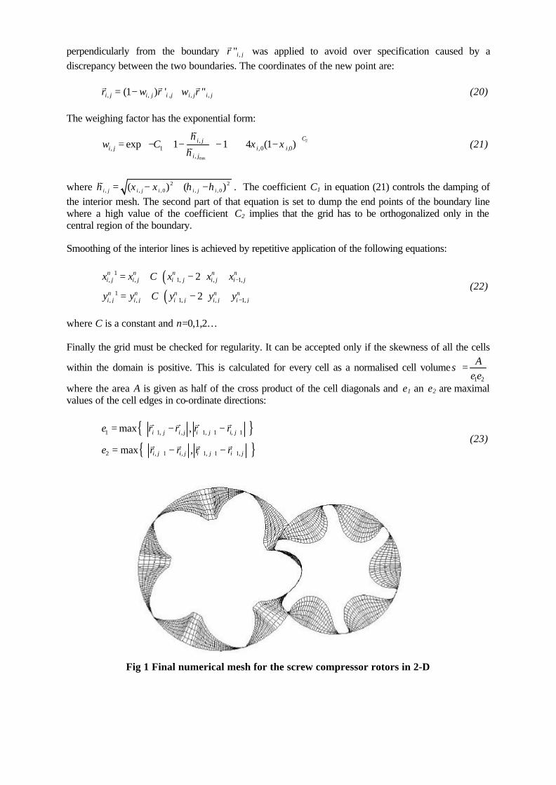
Fig 1 Final numerical mesh for the screw compressor rotors in 2-D

The numerical mesh for the screw compressor rotors of 5/6 configuration produced by this complex method is shown in Fig 1.

2.4 CAD-CFD interface All the methods described in the previous sections have been employed to form a stand alone CAD -CFD interface to produce a regular 3-D mesh of the screw compressor working volume. The interface program is written in Fortran and is called SCORGgg, (Screw COmpressor Rotor Geometry grid generator). More information on the interface is given by Kovacevic et al [5]. The program calculates the meshing rotor coordinates from given rack or rotor curves, by means of two parameter adaptation, and then calculates the grids for both rotors. It also calculates the grids for the inlet and outlet ports and prepares the control parameters necessary for the CFD calculation of the compressor fluid flow. A transfer file is given in ASCII format. This includes the node and cell definitions, regions, boundary conditions, control parameters and post-processing functions. The file can be imported into a commercial CFD package through its pre-processor. These should be able to process control volumes with an arbitrary number of faces. The solution domain can be split into several regions, with separate grid generation in each of them, without the need for grid matching at the region interfaces. Despite the non-matching interfaces, the discretization method is fully conservative and all regions are coupled, so that the solution method converges as well as if the grid was made with one block only. This is very convenient when grids of different topology are generated to obtain the best fit for the geometry of each region. It is then possible to achieve high grid density without the large deformation that would result from a single-block grid. The grid may also be refined locally by subdividing selected cells into a number of smaller cells. The fact that the control volumes may have any number of faces and that the grids do not have to match at interfaces makes it possible to compute flows where the grid moves in some regions while it remains stationary in others.

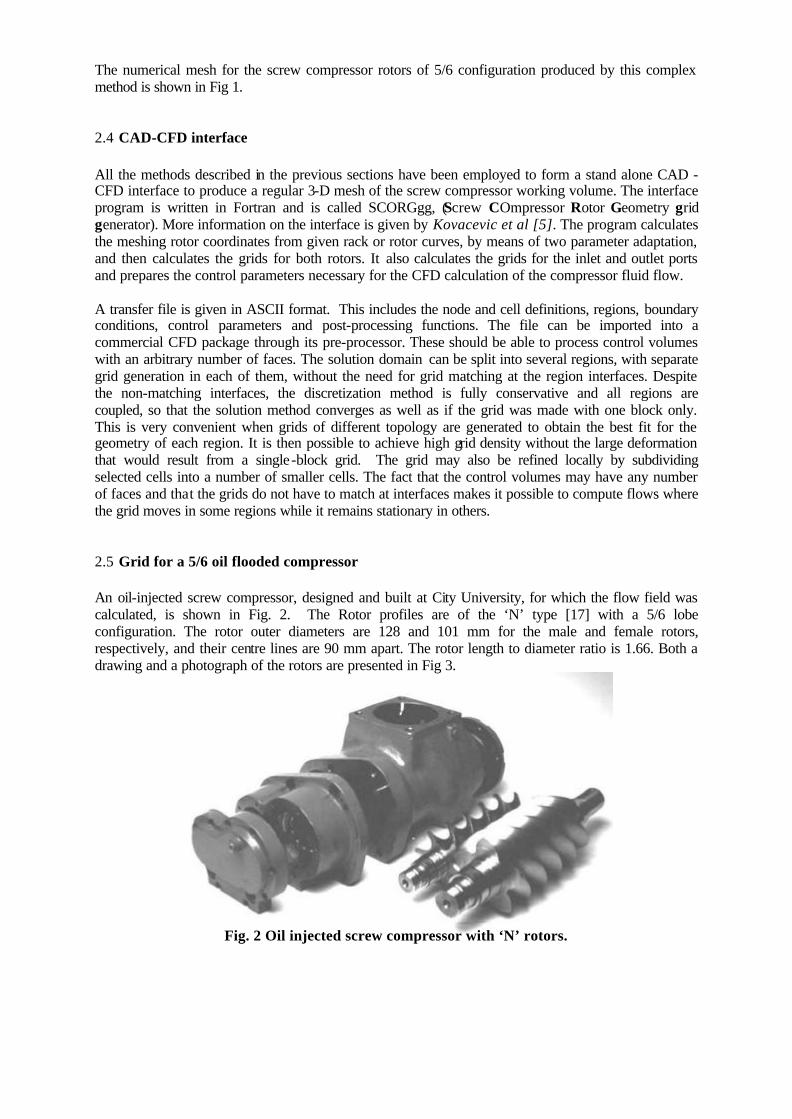
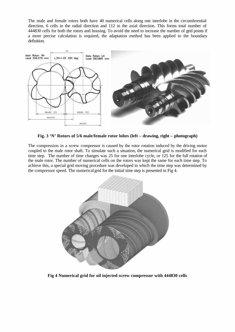
2.5 Grid for a 5/6 oil flooded compressor An oil-injected screw compressor, designed and built at City University, for which the flow field was calculated, is shown in Fig. 2. The Rotor profiles are of the ‘N’ type [17] with a 5/6 lobe configuration. The rotor outer diameters are 128 and 101 mm for the male and female rotors, respectively, and their centre lines are 90 mm apart. The rotor length to diameter ratio is 1.66. Both a drawing and a photograph of the rotors are presented in Fig 3.

Fig. 2 Oil injected screw compressor with ‘N’ rotors.

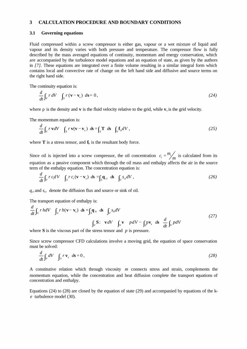
The male and female rotors both have 40 numerical cells along one interlobe in the circumferential direction, 6 cells in the radial direction and 112 in the axial direction. This forms total number of 444830 cells for both the rotors and housing. To avoid the need to increase the number of grid points if a more precise calculation is required, the adaptation method has been applied to the boundary definition.

Fig. 3 ‘N’ Rotors of 5/6 male/female rotor lobes (left – drawing, right – photograph) The compression in a screw compressor is caused by the rotor rotation induced by the driving motor coupled to the male rotor shaft. To simulate such a situation, the numerical grid is modified for each time step. The number of time changes was 25 for one interlobe cycle, or 125 for the full rotation of the male rotor. The number of numerical cells on the rotors was kept the same for each time step. To achieve this, a special grid moving procedure was developed in which the time step was determined by the compressor speed. The numerical grid for the initial time step is presented in Fig 4.

Fig 4 Numerical grid for oil injected screw compressor with 444830 cells

3 CALCULATION PROCEDURE AND BOUNDARY CONDITIONS

3.1 Governing equations Fluid compressed within a screw compressor is either gas, vapour or a wet mixture of liquid and vapour and its density varies with both pressure and temperature. The compressor flow is fully described by the mass averaged equations of continuity, momentum and energy conservation, which are accompanied by the turbulence model equations and an equation of state, as given by the authors in [7]. These equations are integrated over a finite volume resulting in a similar integral form which contains local and convective rate of change on the left hand side and diffusive and source terms on the right hand side. The continuity equation is:

s( ) 0V S

ddV d

dtρ ρ+ − ⋅ =∫ ∫ v v s , (24)

where ρ is the density and v is the fluid velocity relative to the grid, while vs is the grid velocity. The momentum equation is:

s( ) bV S S V

ddV d d dV

dtρ ρ+ − ⋅ = ⋅ +∫ ∫ ∫ ∫v v v v s T s f , (25)

where T is a stress tensor, and fb is the resultant body force.

Since oil is injected into a screw compressor, the oil concentration ii

mc m= is calculated from its

equation as a passive component which through the oil mass and enthalpy affects the air in the source term of the enthalpy equation. The concentration equation is:

s( )i i ci ciV S S V

dcdV c d d s dV

dtρ ρ+ − ⋅ = ⋅ +∫ ∫ ∫ ∫v v s q s , (26)

qci and sci denote the diffusion flux and source or sink of oil. The transport equation of enthalpy is:

s

s

( )

: p

h hV S S V

V V S V

dhdV h d d s dV

dtd

dV pdV d pdVdt

ρ ρ+ − ⋅ = ⋅ + +

∇ + ⋅∇ − ⋅ +

∫ ∫ ∫ ∫

∫ ∫ ∫ ∫

v v s q s

S v v v s (27)

where S is the viscous part of the stress tensor and p is pressure. Since screw compressor CFD calculations involve a moving grid, the equation of space conservation must be solved:

s 0V S

ddV d

dtρ+ ⋅ =∫ ∫ v s , (28)

A constitutive relation which through viscosity µ connects stress and strain, complements the momentum equation, while the concentration and heat diffusion complete the transport equations of concentration and enthalpy. Equations (24) to (28) are closed by the equation of state (29) and accompanied by equations of the k-ε turbulence model (30).

( , )p Tρ ρ= (29)

s

2

s 1 2 3

( ) ( ) ,

( ) ( )

kV S S V

V S S V

dkdV k d d P dV

dtd

dV d d C P C C dVdt k kε

ρ ρ ρε

ε ερε ρε ρ ρε

+ − ⋅ = ⋅ + −

+ − ⋅ = ⋅ + − + ∇ ⋅

∫ ∫ ∫ ∫

∫ ∫ ∫ ∫

v v s q s

v v s q s v (30)

k and ε are the turbulent kinetic energy and its dissipation, while P is production of turbulence

energy. 2t C kµµ ρ ε= is the turbulent viscosity which complements viscosity µ . The constants of

the k- ε turbulence model are: Cµ =0.09, kσ =1, eσ =1.3, C1=1.44, 2C =1.92, C3= -0.33. Standard wall

functions are implemented on the walls

3.2 Specific aspects of the compressor CFD calculation

3.2.1 Oil injection and two phase flow One component of the working fluid in oil-flooded screw compressors is air, which is considered here as a background fluid, while the oil injected into the working chamber is treated as a disperse phase through its concentration. The oil fulfils several functions in the oil injected screw compressor since it seals, lubricates and cools theits working chamber. The influence of oil on the background fluid is shown by two heat flux terms, which are contained in the energy equation. These are defined in equations (32) and (33) by the oil mass and enthalpy. The energy balance for the oil is given in the following form:

( )o o

o con mass

d m TC Q Q

dt= +& & , (31)

The convective heat flux between the air and oil is given by:

( )con o oQ d Nu T Tπ κ= −& , (32) and the heat flux caused by mass transfer between them is:

omass

dmQ L

dt=& . (33)

where L is the specific enthalpy of vaporization In theseequations Co, To and k are the specific heat, temperature and the thermal conductivity of oil. The Sauter mean diameter do is the parameter which determines heat transfer between the phases. In the case of an oil injected screw compressor, its value is between 10 and 50 µm. More details about this are given by Stosic at al [15].

3.2.2 Boundary conditions A novel treatment of compressor boundaries was introduced in the numerical calculation as follows. The compressor was positioned between relatively small suction and discharge receivers. Therefore, the compressor system was separated from its surroundings only by walls. It communicates with the surroundings through the mass and energy source or sink placed in these receivers to maintain constant suction and discharge pressures. The compressor intake and discharge flows and pressure

change within the compressor are then caused solely by the rotor movement. This allows the compressor calculation to start from rest with relatively coarse initial conditions and establish a full solution after only a fraction of a compressor cycle. Such an approach is completely different from the standard inlet and outlet boundary conditions, or pressure boundary condition. The first would not allow a flow reversal at the compressor discharge, while the latter would be prohibitively slow due to the unsteady character of the compressor process. The novel approach therefore introduces additional stability to accelerate calculation. The procedure secures full and precise control of the pressures in both reservoirs and reduces the calculation time required by a factor of five compared with any other approach. The same was used for the boundary conditions in the oil injection port. 3.3 Calculation of the compressor performance Once the velocity and pressure fields in the compressor are calculated, the compressor volume flow is obtained at the screw compressor suction as a scalar product of the fluid velocity and corresponding surface vectors for each cell. When multiplied by the corresponding density and integrated over the entire cross section, compressor volume flow gives the compressor mass flow. Finally, the volume and mass flows were averaged for all time steps. The same procedure was applied to calcula te the outlet mass flow. Mass flow of the oil through the oil injection port was calculated from the mass concentration of oil in its port. The inlet air and oil injected mass flows should be equal to the outlet mass flow of the mixture for steady working conditions. Since the pressure in the working chamber does not vary too much in one interlobe within one time step, it was sufficiently accurate to average the pressure values arithmetically in each working chamberto plot pressure-shaft angle, p-α diagrams for all interlobes in all the time steps of the working cycle. However, the calculation of the torque and forces acting on the rotors requires pressure values in each cell of the working chamber to be considered. The forces acting on the rotor, which are caused by pressure in the working chamber, are calculated as a product of the pressure at the rotor face cell boundary and the corresponding cell area vector. The resultant force has three components, one in the rotor axial and two in the transverse directions. The cross product of the force and its coordinate forms a force moment, the components of which act in three directions. Two of them serve to calculate axial and radial force reactions in the suction and discharge bearings, while the third component is the torque acting on both, the male and female rotors. To obtain integral radial and axial forces and torque, the cell values are summed over the entire surfaces of both rotors. Once obtained, the torque is used to calculate the compressor power transmitted to the rotor shaft as a product of the torque and shaft speed. The shaft power should correspond to the indicated power calculated from the p-V diagram. Compressor specific power is calculated as the ratio of the input power to the compressor volume flow. The volumetric efficiency is calculated as the ratio of the compressor volume flow to the compressor theoretical displacement and the compressor adiabatic efficiency is calculated as the ratio of the compressor theoretical adiabatic power: to either the shaft or indicated power.

4 RESULTS AND DISCUSSION 4.1 Compressor measurements In the absence of flow field measurements in the compressor chamber, the experimentally obtained pressure history within the compressor cycle and the measured air flow and compressor power served

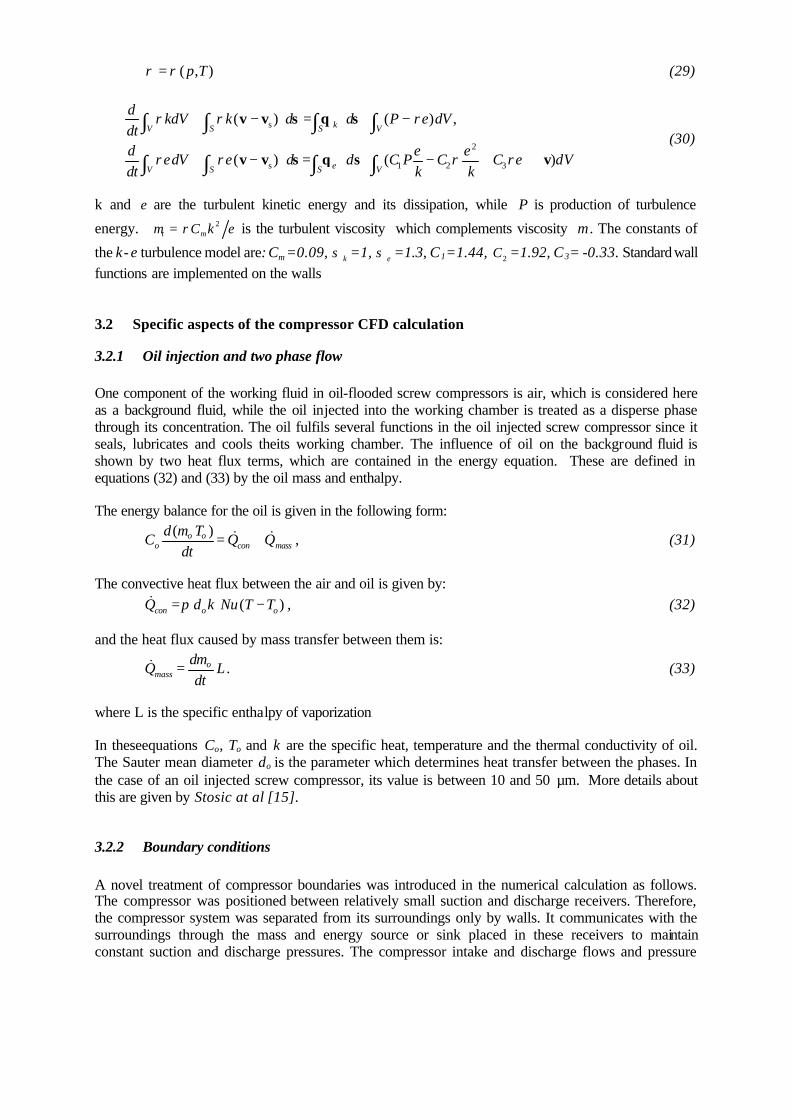
as a valuable basis to validate the results of the CFD calculation. The 5/6 oil flooded compressor, already described, was tested to obtain this data on a rig which has been certified by Lloyd’s of London as fully meeting Pneurop/Cagi requirements for screw compressor acceptance tests. The compressor was tested according to the procedures specified in ISO 1706 and the delivered flow was measured in accordance with BS 5600. High accuracy test equipment was used for the measurement of all relevant parameters. All measurements were made by transducers and both recorded and processed in a computerized data logger for real time presentation. A screen record of the compressor measurement is given in Fig 6. A Diesel engine of 100 kW maximum power output, which can operate at variable speed, was used as the prime mover. This permits the testing of oil-flooded screw compressors with discharge rates of up to 16 m3 /min.

Fig. 5 Compressor test layout and the computer screen

4.2 CFD calculation A numerical solution of the system of equations was obtained from the CFD solver ‘Comet’, which is developed by the Institute of Computational Continuum Mechanics GmbH. This code is applicable not only to fluid flow but also for solid body analysis. It also meets the needs of coupled computation of gas and liquid flow including moving surfaces, non-Newtonian fluids, flows with both highly compressible as well as incompressible regions, flows with moving boundaries and particle flows. Hence, it contains all the essential features needed to obtain the ultimate aims of full machine simulation. All additional terms described in previous chapter were introduced through user functions. The numerical mesh produced by the stand alone grid generator was automatically transferred to the CFD solver together with all control parameters and user functions. To establish a full range of working conditions and to obtain an increase of pressure from 1 to 5, 7 or 9 bars between the compressor suction and discharge with a numerical mesh of nearly 450000 cells, only 25 time steps were required, following which a further 25 time steps were needed to complete a full compressor cycle. Each time step needed about 30 minutes running time on an 800 MHz AMD Athlon processor. The computer memory required was about 450 MB.

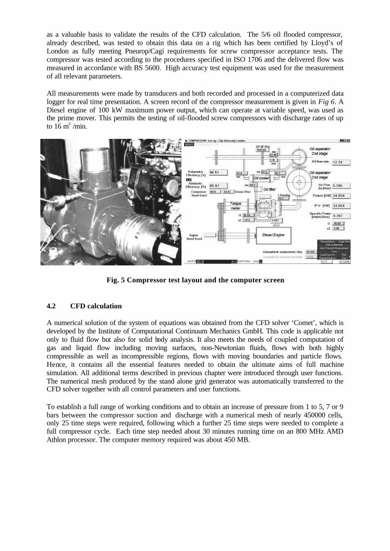
4.3 Comparison of the CFD results and experimental data Results of the CFD calculation of an oil injected air compressor are presented in Figs 6-9. Variation of pressure within the working cycle calculated from the CFD estimate is compared with measured values in Fig 10 and in Tab 1. The forces acting on the rotors and the bearing forces are shown in Figs 11 and 12. In Fig 6 and 7 the velocity vectors in two cross sections and two different time steps in the axial section are compared respectively. The high values of velocity in gaps both between the rotors and their housing and between the two rotors generated by the sharp pressure gradient through the clearances are clearly distinguished from the velocities in the highly turbulent regions in the interlobes where the movement is relatively slower. Velocity changes in space, as presented in two cross sections in the Fig 6, and through change in time are caused only by the movement of the numerical mesh, which follows the rotation of the rotors. Velocity field in the axial section is shown in Fig 7 .

Fig. 6 Velocity vectors in the two compressor cross section Left – suction port, Right – working chamber

Fig. 7 Velocity vectors in the compressor axial section

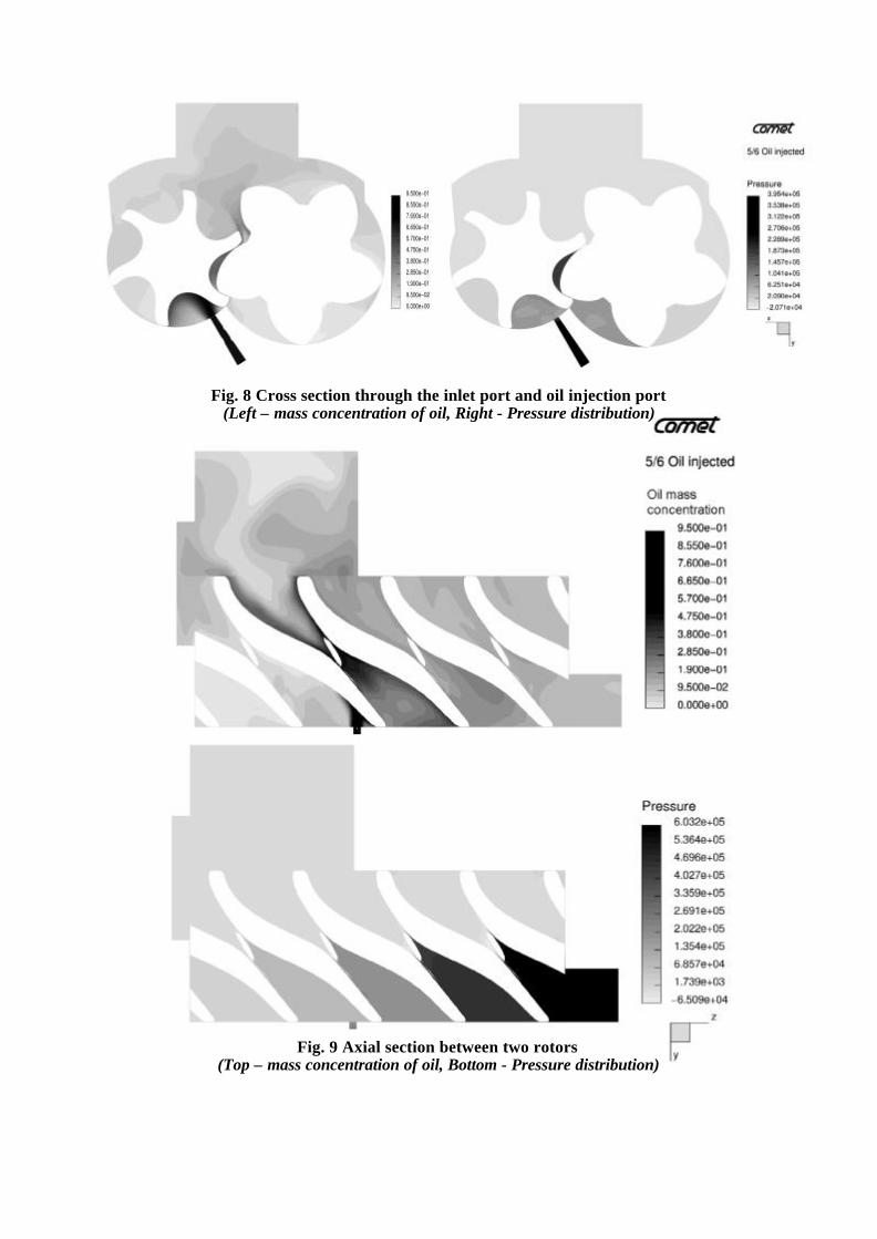
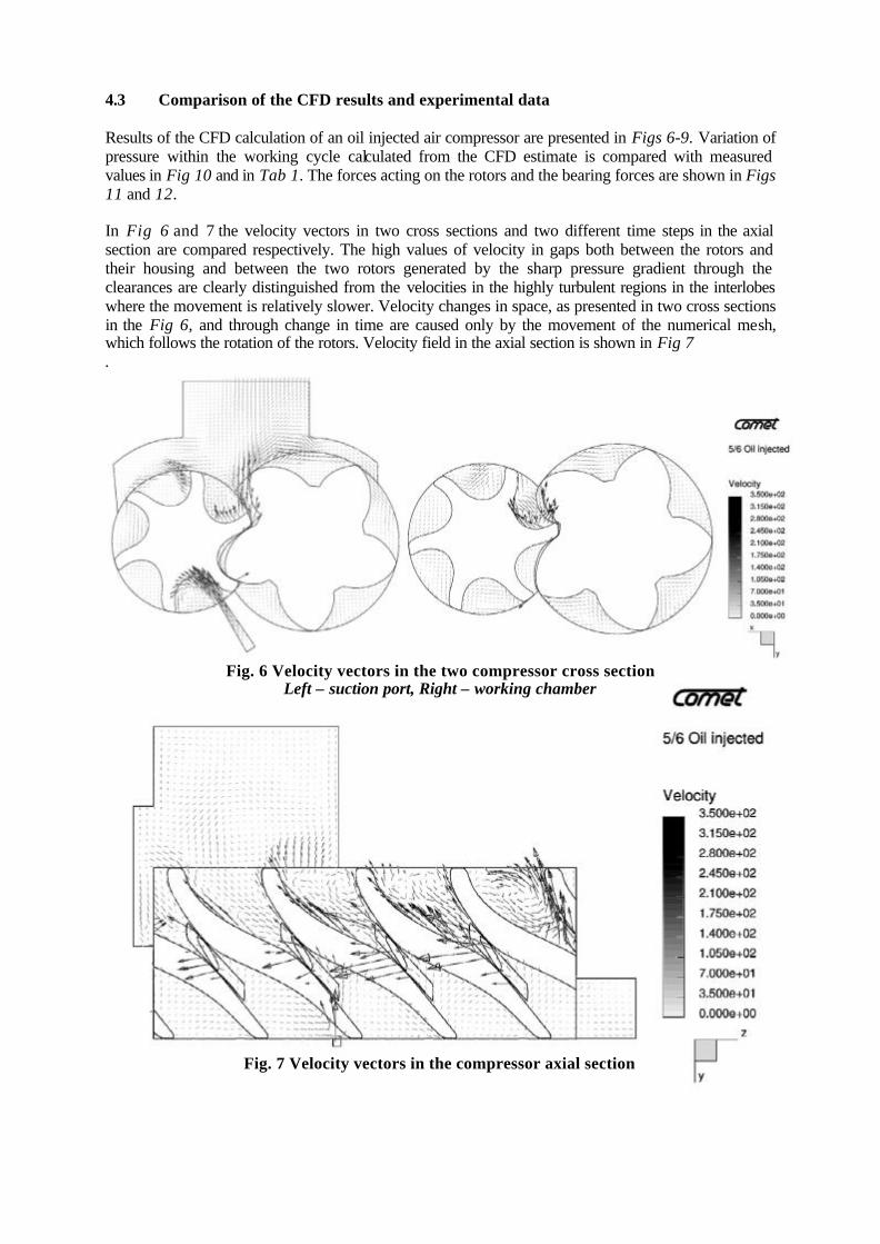
Fig. 8 Cross section through the inlet port and oil injection port (Left – mass concentration of oil, Right - Pressure distribution)

Fig. 9 Axial section between two rotors (Top – mass concentration of oil, Bottom - Pressure distribution)

The oil and pressure distribution in the cross section with the oil injection port are shown in Fig 8. The flow of oil within the machine is clearly shown in the axial section through the rotors, presented in Fig 9, on the top diagram. The pressure rise within the machine when rotating at 5000 rpm with a discharge pressure of 7 bar absolute is shown on the bottom of the diagram. The estimated thermodynamic and flow properties presented in previous figures were later used for calculation of the overall parameters of the analysed screw compressor.

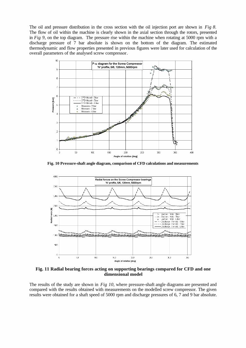
Fig. 10 Pressure-shaft angle diagram, comparison of CFD calculations and measurements

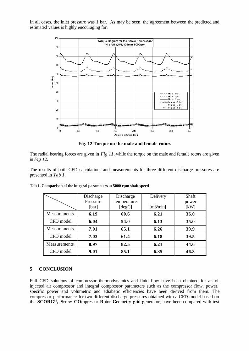
Fig. 11 Radial bearing forces acting on supporting bearings compared for CFD and one dimensional model

The results of the study are shown in Fig 10, where pressure-shaft angle diagrams are presented and compared with the results obtained with measurements on the modelled screw compressor. The given results were obtained for a shaft speed of 5000 rpm and discharge pressures of 6, 7 and 9 bar absolute.

In all cases, the inlet pressure was 1 bar. As may be seen, the agreement between the predicted and estimated values is highly encouraging for.

Fig. 12 Torque on the male and female rotors

The radial bearing forces are given in Fig 11, while the torque on the male and female rotors are given in Fig 12. The results of both CFD calculations and measurements for three different discharge pressures are presented in Tab 1. Tab 1. Comparison of the integral parameters at 5000 rpm shaft speed

Discharge Pressure

[bar]

Discharge temperature

[degC]

Delivery

[m3/min]

Shaft power [kW]

Measurements 6.19 60.6 6.21 36.0

CFD model 6.04 54.0 6.13 35.0

Measurements 7.01 65.1 6.26 39.9

CFD model 7.03 61.4 6.18 39.5

Measurements 8.97 82.5 6.21 44.6 CFD model 9.01 85.1 6.35 46.3

5 CONCLUSION Full CFD solutions of compressor thermodynamics and fluid flow have been obtained for an oil injected air compressor and integral compressor parameters such as the compressor flow, power, specific power and volumetric and adiabatic efficiencies have been derived from them. The compressor performance for two different discharge pressures obtained with a CFD model based on the SCORGgg, Screw COmpressor Rotor Geometry grid generator, have been compared with test

results obtained from a real compressor. The good agreement between predicted and measured performance is a strong indication that CFD analysis can be developed further as a powerful tool for the design and optimisation of screw compressors.

REFERENCES 1. Demirdzic I, Peric M, 1990, Finite Volume Method for Prediction of Fluid flow in Arbitrary Shaped

Domains with Moving Boundaries, Int. J. Numerical Methods in Fluids Vol 10, 771 2. Demirdzic I, Lilek Z, Peric, M, 1993, A Collocated Finite Volume Method for Predicting Flows at All

Speeds, Int. J Numerical Methods in Fluids, Vol. 16, 1029 3. Demirdzic I, Muzaferija S, 1995, Numerical Method for Coupled Fluid Flow, Heat Transfer and Stress

Analysis Using Unstructured Moving Mesh with Cells of Arbitrary Topology, Comp. Methods Appl. Mech Eng, Vol 125 235-255

4. Ferziger J H, Peric, M, 1996, Computational Methods for Fluid Dynamics, Springer, Berlin

5. Kovacevic A, Stosic N, Smith I. K, 1999, Development of CAD-CFD Interface for Screw Compressor Design, International Conference on Compressors and Their Systems, London, IMechE Proceedings, 757

6. Kovacevic A, Stosic N, Smith I. K, 2000,: The CFD Analysis of a Screw Compressor Suction, International Compressor Engineering Conference at Purdue, 909

7. Kovacevic A, Stosic N, Smith I. K, 2000, Grid Aspects of Screw Compressor Flow Calculations, Proceesings of the ASME Congress- 2000, Advanced Energy Systems Division, Vol. 40, 83

8. Lehtimaki R, 2000, An Algebraic Boundary Orthogonalization Procedure for Structured Grids, International Journal for Numerical Methods in Fluids, Vol. 32, 605-618

9. Liseikin V.D, 1999, Grid generation Methods, Springer-Verlag

10. Muzaferija S, 1994, Adaptive Finite Volume Method for Flow Prediction Using Unstructured Meshes and Multigrid Approach, PhD Thesis, Imperial College of Science, Technology & Medicine, London

11. Peric, M, 1985, A Finite Volume Method for the Prediction of Three Dimensional Fluid Flow in Complex Ducts, PhD Thesis, Imperial College of Science, Technology & Medicine, London

12. Shih T. I. P, Bailey R. T, Ngoyen H.L, Roelke R.J, 1991, Algebraic Grid Generation For Complex Geometries, International Journal for Numerical Methods in Fluids, Vol. 13, 1-31

13. Smith R.E, 1982, Algebraic Grid Generation, from Numerical Grid Generation, ed. By Thomson J.FG, Elsevier Publishing Co, 137

14. Steinthorsson E, Shih T. I. P, Roelke R. J, 1992, Enhancing Control of Grid Distribution In Algebraic Grid generation Generation, International Journal for Numerical Methods in Fluids, Vol. 15, 297-311

15. Stosic N, Milutinovic Lj, Hanjalic K, Kovacevic A, 1992, Investigation of the Influence of Oil Injection upon the Screw Compressor Working Process, Int.J.Refrig. 15,4,206

16. Stosic N, Smith I. K, Zagorac S, 1996, CFD Studies of Flow in Screw and Scroll Compressors, XIII Int. Conf on Compressor Engineering at Purdue

17. Stosic N, 1998, On Gearing of Helical Screw Compressor Rotors, Proc IMechE, Journal of Mechanical Engineering Science, Vol.212, 587

18. Thompson J.F, Soni B, Weatherrill N.P, 1999, Handbook of Grid generation, CRC Press