Embed Size (px)
Citation preview
CFD INVESTIGATION OF THE EFFECT OF SPINNERET GEOMETRY ON
THE FLOW BEHAVIOR OF MULTIPHASE POLYMERIC FLUIDS
by
DİLAY ÜNAL
Submitted to the Graduate School of Engineering and Natural Sciences
in partial fulfillment of
the requirements for the degree of
Master of Science
Sabancı University
August 2014
CFD INVESTIGATION OF THE EFFECT OF SPINNERET GEOMETRY ON
THE FLOW BEHAVIOR OF MULTIPHASE POLYMERIC FLUIDS
APPROVED BY:
Assoc. Prof. Dr. Mehmet Yıldız ..............................................
(Thesis Supervisor)
Prof. Dr. Yusuf Z. Menceloğlu ..............................................
(Thesis Supervisor)
Assoc. Prof. Dr. Ali Koşar ..............................................
Asst. Prof. Dr. Fevzi Cebeci ..............................................
Asst. Prof. Dr. Serkan Ünal ..............................................
DATE OF APPROVAL : 06/08/2014

© Dilay Ünal 2014
All Rights Reserved

“Of course there is no formula for success, except perhaps an unconditional acceptance
of life and what it brings.”
Arthur Rubinstein
v
CFD Investigation of the Effect of Spinneret Geometry on the Flow Behavior of
Multiphase Polymeric Fluids
Dilay Ünal
MAT, M.Sc. Thesis, 2014
Thesis Supervisors : Prof. Dr. Yusuf Menceloğlu, Assoc. Prof. Dr. Mehmet Yıldız
Keywords : CFD, FLUENT, multiphase flow, spinneret
ABSTRACT
Nano or micro particle integrated polymeric fibers are commonly produced via so-
called wet spinning process. During the process, particle containing polymer solution is
exposed to high shear stresses while passing through the spinneret holes, and high shear
stresses give rise to increased viscosity (shear thickening). In the present work, it was
aimed to investigate parameters that affect the flow behavior of shear thickening fluids.
The fluid considered in the simulations was prepared by dispersing silica nanoparticles
in poly(ethyleneglycol), and the resulting fluid was a complex fluid which shows shear
thinning until a certain shear rate, and above that shear rate it shows shear thickening.
The effects of various parameters on the flow properties of the fluid have been
investigated over a wide range of conditions. The variables studied are: geometry
(reservoir depth, channel length, contraction width, edge roundness), velocity (0.02-0.12
m/s). A two-dimensional simulation model based on an Eulerian-Eulerian multiphase
approach is considered to simulate particle containing polymeric fluid. The governing
equations and constitutive relations for both phases are solved using the finite volume
method, by employing the FLUENT software of ANSYS Workbench. Since it would be
computationally too expensive to model the entire spinneret, only one single hole was
considered as the computational domain. It was found that reservoir depth and channel
length have slight effect on the viscosity but at the same time contraction width and
roundness of the edge of the contraction has a significant effect on the viscosity profile.
Besides, by increasing velocity fluid viscosity increased as well.
vi
Spinneret Geometrisinin Çok Fazlı Polimerik Akışkanların Akış Özellikleri
Üzerine Etkilerinin Hesaplamalı Akışkanlar Dinamiği Yöntemi ile İncelenmesi
Dilay Ünal
MAT, M.Sc. Tezi, 2014
Tez Danışmanları : Prof. Dr. Yusuf Menceloğlu, Doç. Dr. Mehmet Yıldız
Anahtar Kelimeler : Hesaplamalı Akışkanlar Dinamiği, FLUENT, çok fazlı akış
ÖZET
Nano veya mikro boyutta parçacık içeren polimerik fiberler, yaş çekim yöntemi adı
verilen bir proses ile üretilebilmektedir. Bu proses esnasında, parçacık içeren polimer
solüsyonu, spinneret (düze) adı verilen mikron boyutlarındaki deliklerden geçirilirken,
yüksek kayma gerilimine maruz kalırlar. Polimer solüsyonu üzerine etki eden bu yüksek
kayma gerilimi viskozite artışına sebep olur. Bu tez kapsamında, kayma kalınlaşması
gösteren polimerik sıvıların akış özelliklerine etki eden parametreler incelenmiştir.
Simülasyonlarda kullanılan akışkan, silika nanoparçacıklarının poli(etilenglikol)
içerisinde dağıtılmasıyla hazırlanmış olup, hazırlanan bu numune, belirli bir kayma
geriliminin altında kayma incelmesi gösterirken, o kayma geriliminin üzerinde ise
kayma kalınlaşması göstermektedir. İncelenen parametreler: geometri (rezervuar
derinliği, kanal uzunluğu, kısılma alanının genişliği, ve köşelerin yuvarlatılması), akış
hızı (0.03-0.12 m/s). Simülasyonlar iki boyutlu bir geometri kullanılarak, Eulerian-
Eulerian metodu kullanılarak modellenmiştir. Akış özelliklerini tanımlayan denklemler,
sonlu hacimler metodu kullanılarak, ANSYS FLUENT programı ile çözülmüştür.
Simülasyonların maliyeti düşünülerek, tüm spinnereti modellemek yerine, yalnızca bir
adet delik baz alınmış ve hesaplamalar onun üzerinde yapılmıştır. Elde edilen
sonuçların ışığında, rezervuar derinliği ve kanal uzunluğunun viskozite üzerine çok az
etkisi olduğu görülmüştür. Bunun yanında, kısılma alanının genişliği ve köşelerin
keskinliğinin ise viskozite profili üzerinde hatırı sayılır ölçüde değişikliğe sebep olduğu
gözlemlenmiştir. Ayrıca, akış hızının artırılmasıyla da viskozitenin önemli ölçüde arttığı
görülmüştür.

vii
ACKNOWLEDGEMENTS
First of all, I would like to express my special thanks to my supervisors Professor
Mehmet Yıldız and Professor Yusuf Menceloğlu for their patient guidance,
encouragement and advices that they provided throughout my time as their student.
I would like to thank to Professors Ali Koşar, Fevzi Cebeci and Serkan Ünal for being
my jury members and for their valuable comments on my thesis.
I would like to thank Sabancı University for funding my education for two years and I
would also like to acknowledge Republic of Turkey, Ministry of Science, Industry and
Technology and AKSA Akrilik A.Ş. for providing the funding for this research project.
Special thanks to all MAT faculty members and MAT-Grad family. Completing this
study would have been all the more difficult without the support and friendship
provided by them.
I would like to express my sincere gratitude to my friends who were always beside me
and supporting me for two years. Ayça Ürkmez, for being a wonderful friend, and a
sister, and the one whom I can speak without words. Nihan Ongun, for being an
awesome roommate and sharing all of those laughter and cry. Tuğçe Akkaş, for all
those moments we spent caring each other. Pelin Güven, for being such a unique
personality in my life and for cookies of course. Ece Belen, for her friendship, and
Nesibe Ayşe Doğan, for her valuable existence with her always smiling face.
Last but not least, I would like to especially thank my family for always being there,
supporting and loving me. I am grateful for everything that they have done for me.
Selvet Ünal, for being such a wonderful person and mother. Nilay Ünal for being more
than a sister, a part of me, who I know will always be there no matter what. My
brothers, Dilhan and Emirhan Ünal for their existence and love. I am sure that I
wouldn’t be the same person, if I weren’t the eldest sister of them. I would like to thank
my grandfather, Ali Ünal, for always supporting me and believing in me from the
beginning of my life, and my heavenly grandmother, Selime Ünal, my precious Biko, I
am sure that no words could describe her happiness and proud if she was here and saw
me graduating. Moreover, my other heavenly grandmother and grandfather, even
though I have never met them, I am quite sure that they would be so proud of their
grandchild, and of their daughter for raising me and my siblings.

viii
Lastly but mostly, I would like to thank Tayfun Serttan, my fiancé, the love of my life,
for his existence, support, patience and endless love. It would not be possible without
him to survive last two years and complete this thesis. He was always there, no matter
what, during all my best and worst times, and I know that he will always be there, till
the end of our lives. I lovingly dream about the day that, you, me and our children
reading this, laughing, and feeling blessed once more.
ix
TABLE OF CONTENTS
ABSTRACT ...................................................................................................................... v
ÖZET ............................................................................................................................... vi
LIST OF FIGURES ......................................................................................................... xi
LIST OF TABLES .......................................................................................................... xii
ABBREVIATIONS ....................................................................................................... xiii
1. INTRODUCTION ........................................................................................................ 1
1.1. Motivation .............................................................................................................. 1
1.2. Outline of the Thesis .............................................................................................. 2
2. BACKGROUND .......................................................................................................... 3
2.1. Rheology Basics .................................................................................................... 3
2.2. Computational Fluid Dynamics for Multiphase Fluid Flows ................................ 5
3. FORMULATION OF CFD MODEL ........................................................................... 9
3.1. Conservation of Mass ............................................................................................ 9
3.2. Conservation of Momentum .................................................................................. 9
3.2.1. Fluid-Fluid Momentum Equation ................................................................. 10
3.2.2. Fluid-Solid Momentum Equation ................................................................. 10
3.3 Carrier Fluid Viscosity .......................................................................................... 10
3.4. The Pressure Correction Equation ....................................................................... 11
3.5. Volume Fraction Equation ................................................................................... 11
3.6. Fluid-Solid Exchange Coefficient ....................................................................... 11
3.7. Solid Shear Stresses ............................................................................................. 12
3.7.1. Collisional Viscosity ..................................................................................... 12
3.7.2. Kinetic Viscosity ........................................................................................... 12
3.7.3. Bulk Viscosity ............................................................................................... 13
3.8. Solver Theory ...................................................................................................... 13
x
4. DESCRIPTION OF CFD SIMULATIONS ............................................................... 15
4.1. Simulation of Validation Case ............................................................................. 15
4.2. Simulations of Single Phase Fluid Flow and Two-Phase Solid-Liquid Flow ..... 16
4.2.1. Geometry ...................................................................................................... 16
4.2.2. Mesh .............................................................................................................. 17
4.2.3. Material Properties ........................................................................................ 17
4.2.4. Description of the Numerical Model ............................................................ 18
5. RESULTS AND DISCUSSION ................................................................................. 20
5.1. Validation Case .................................................................................................... 20
5.2. Two-Phase Solid-Liquid Flow ............................................................................. 22
5.2.1. Mesh Dependency Analysis .......................................................................... 22
5.2.2. Parametric Study ........................................................................................... 22
5.2.2.1. Geometry ............................................................................................... 22
5.2.2.2. Fluid Velocity ........................................................................................ 32
6. CONCLUDING REMARKS ...................................................................................... 35
6.1. Future Work ......................................................................................................... 35
APPENDIX A ................................................................................................................. 36
REFERENCES ............................................................................................................... 38
xi
LIST OF FIGURES
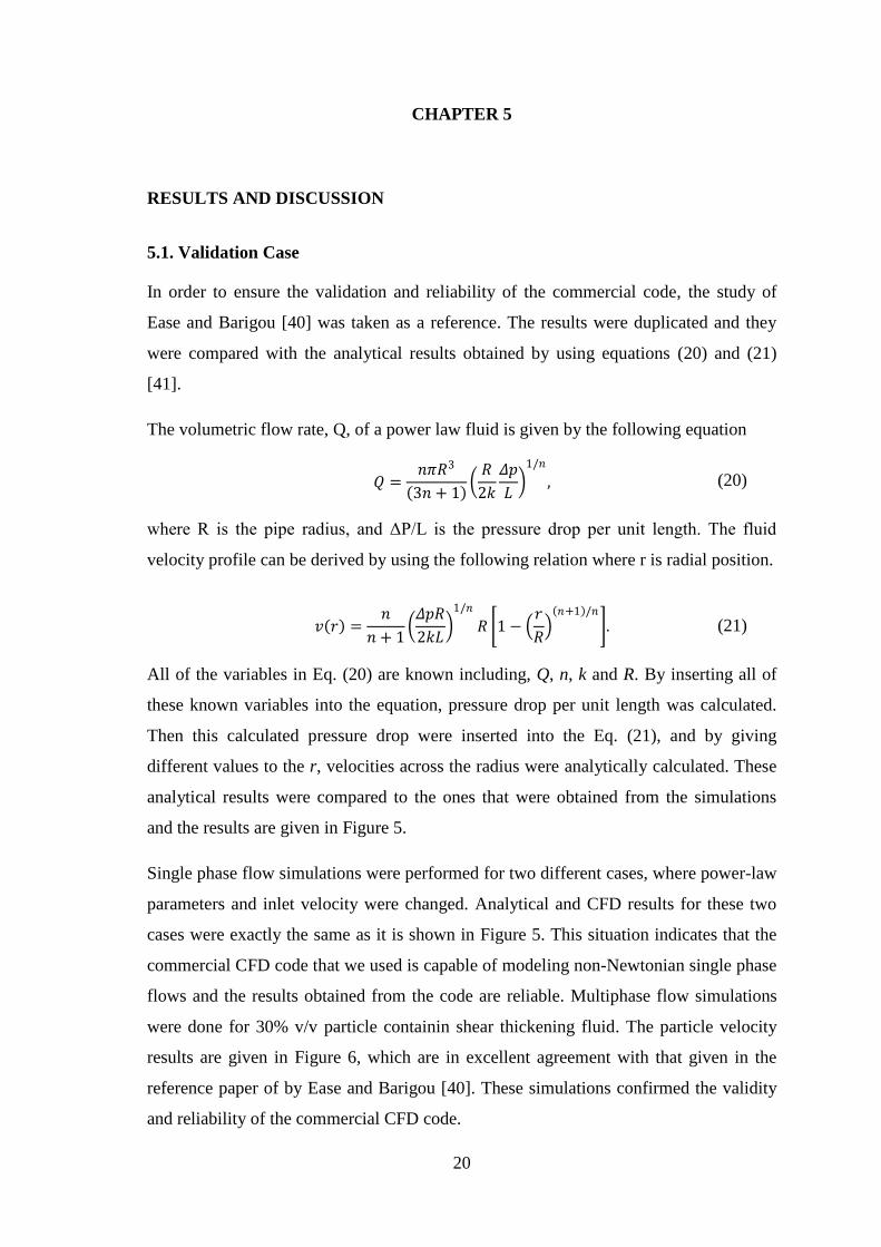
Figure 1. A representative image of a spinneret ............................................................. 16
Figure 2. Geometry of the computational domain .......................................................... 16
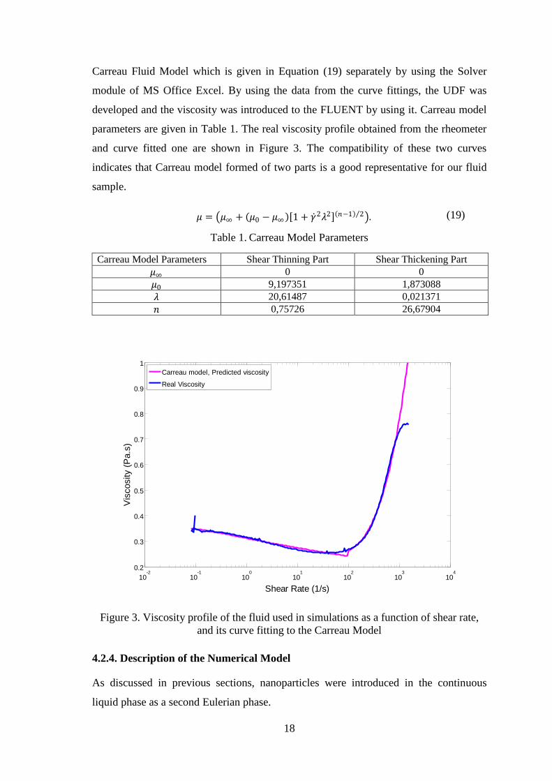
Figure 3. Viscosity profile of the fluid used in simulations as a function of shear rate,
and its curve fitting to the Carreau Model ...................................................................... 18
Figure 4. Boundaries of the computational domain ........................................................ 19
Figure 5. Comparison of analytical and CFD velocity profiles for a power law fluid
flowing alone: (k=0.16 Pa.sn, n=0.81), Vin=66mm/s; (k=0.75 Pa.s
n, n=0.71),
Vin=33mm/s .................................................................................................................... 21
Figure 6. Normalised solid-phase velocity profile in shear thickening carrier fluid:
(k=0.75 Pa.sn, n=0.71); d=2mm, ρs=1020 kg/m
3, Cs=0.30; Vin= 125 mm/s ................... 21
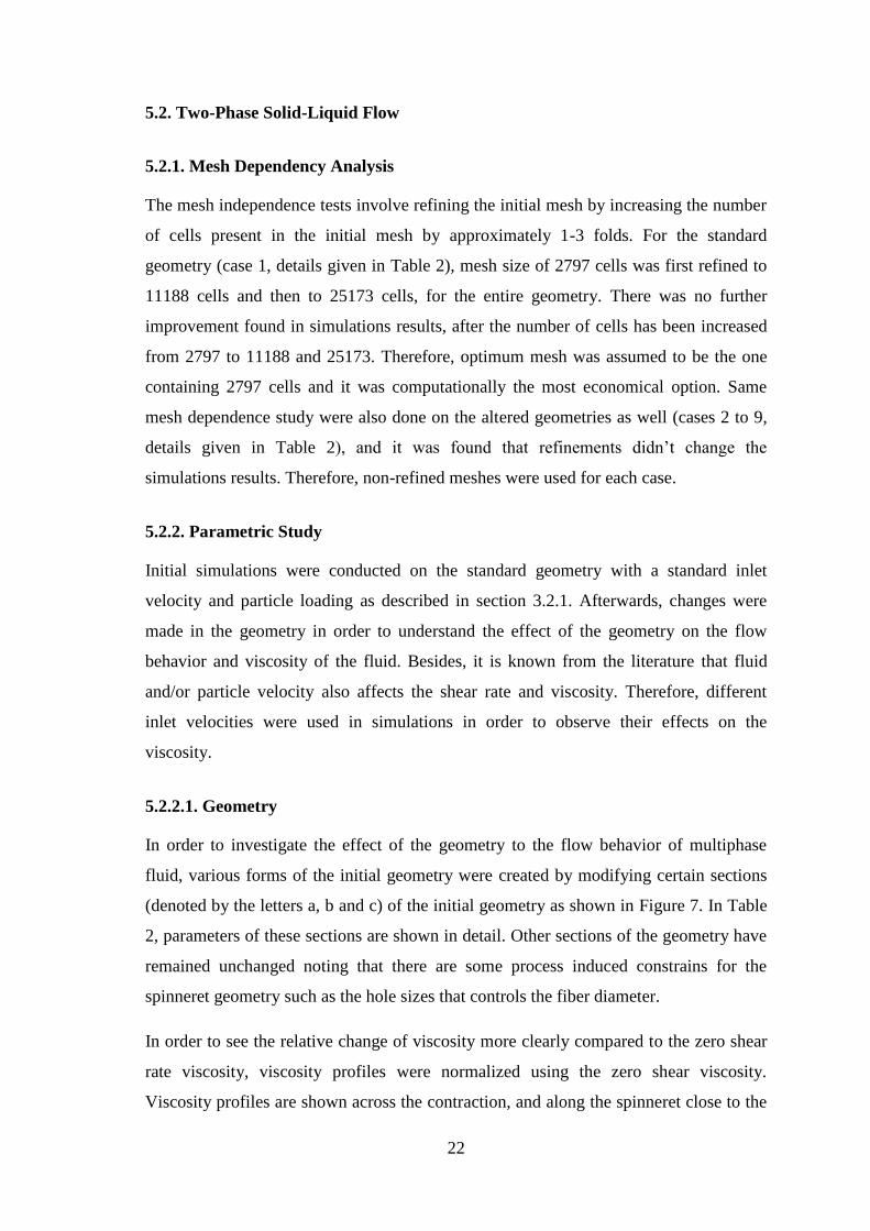
Figure 7. Parts of the geometry that were changed and lines that viscosity was observed
........................................................................................................................................ 23
Figure 8. Effect of the reservoir depth on the viscosity profile along the Line-1 ........... 24
Figure 9. Effect of the reservoir depth on the viscosity profile across the contraction .. 24
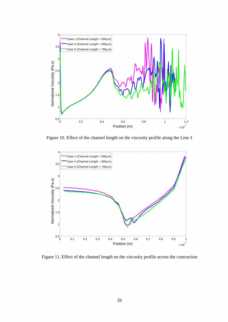
Figure 10. Effect of the channel length on the viscosity profile along the Line-1 ......... 26
Figure 11. Effect of the channel length on the viscosity profile across the contraction . 26
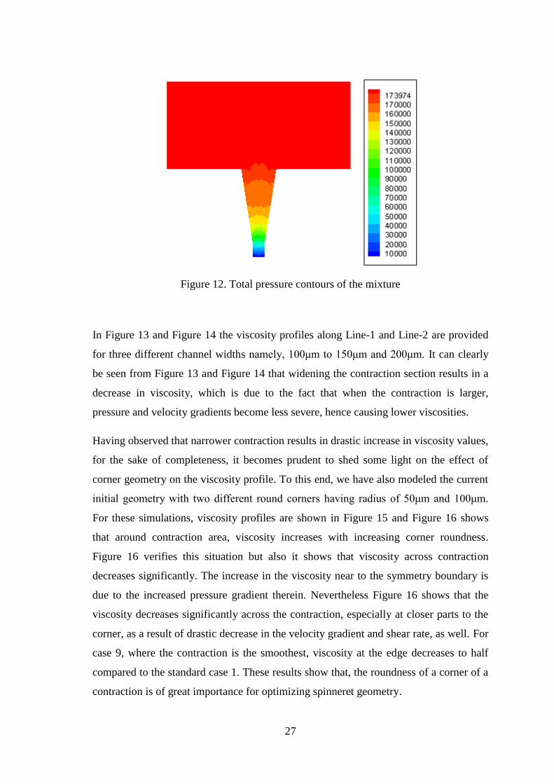
Figure 12. Total pressure contours of the mixture .......................................................... 27
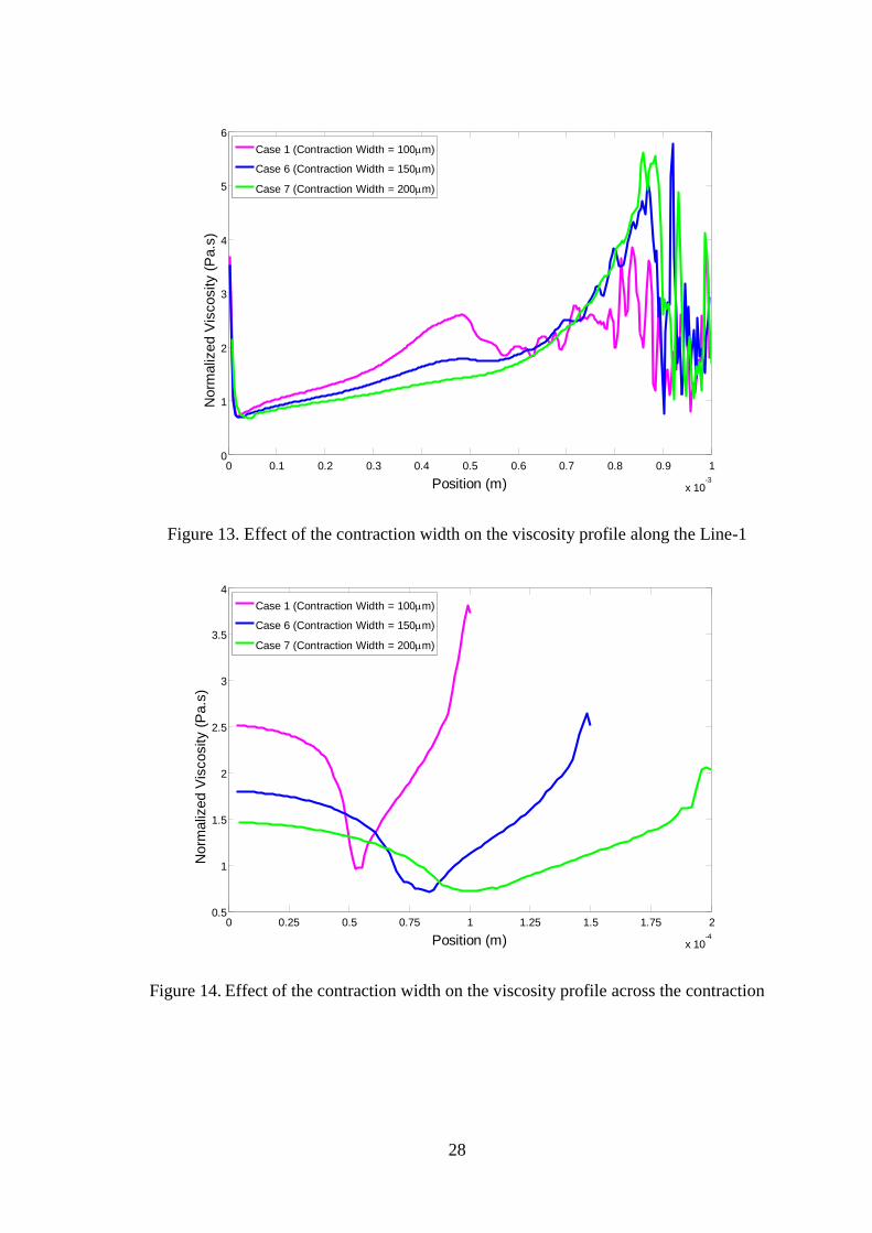
Figure 13. Effect of the contraction width on the viscosity profile along the Line-1 ..... 28
Figure 14. Effect of the contraction width on the viscosity profile across the contraction
........................................................................................................................................ 28
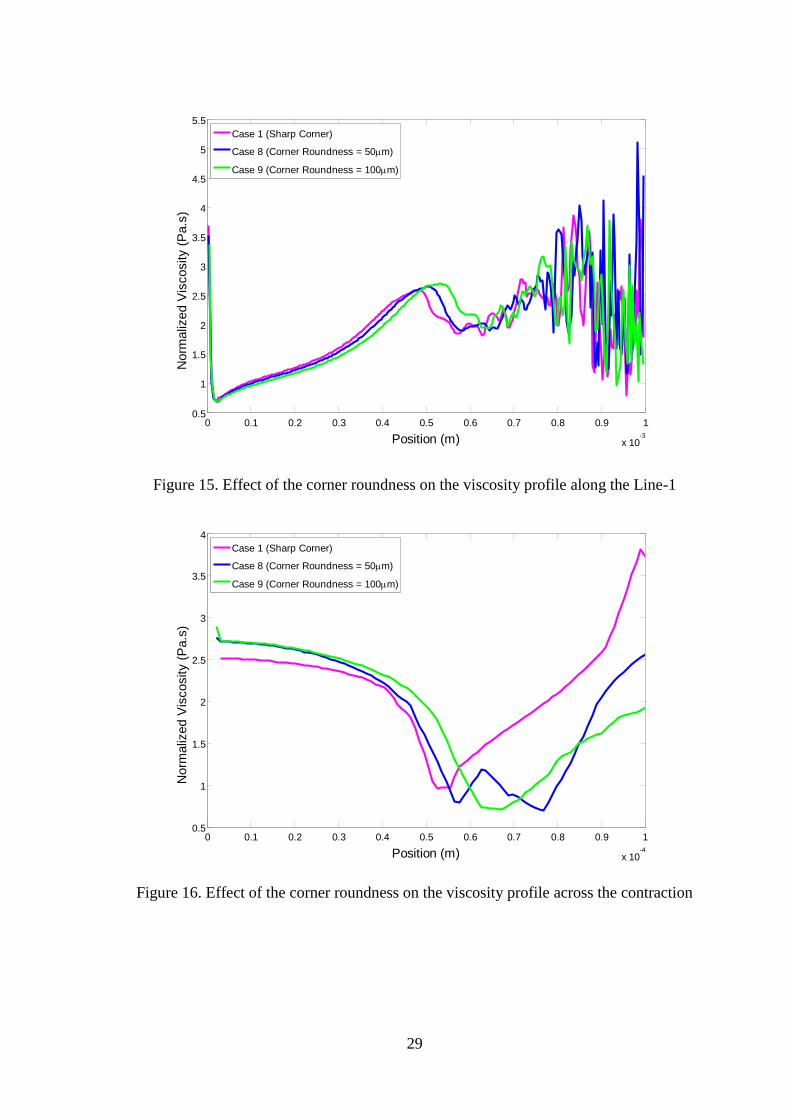
Figure 15. Effect of the corner roundness on the viscosity profile along the Line-1 ..... 29
Figure 16. Effect of the corner roundness on the viscosity profile across the contraction
........................................................................................................................................ 29
Figure 17. Velocity contours of the mixture ................................................................... 30
Figure 18. Dynamic pressure contours of the mixture .................................................... 30
Figure 19. Viscosity contours of the mixture ................................................................. 31
Figure 20. Effect of the velocity on the viscosity profile along the Line-1 .................... 33
Figure 21. Effect of the velocity on the viscosity profile across the contraction ........... 33
Figure 22. Viscosity contours of the mixture where inlet velocity boundary condition is
used as 0.0019 m/s .......................................................................................................... 34
xii
LIST OF TABLES
Table 1. Carreau Model Parameters ............................................................................... 18
Table 2. Dimensions of the geometry used at simulations ............................................. 23
Table 3. Different velocities used and their correspondence to mass flow rates ............ 32
xiii
ABBREVIATIONS
CFD Computational Fluid Dynamics
ODT Order-Disorder Transition
PEG Poly(ethyleneglycol)
UDF User Defined Function
2D Two Dimensional

xiv
To my beloved mom...
1
CHAPTER 1
INTRODUCTION
1.1. Motivation
Natural fibers such as cotton, wool, and silk have been used by humans since ancient
times. Patenting of artificial silk in 1885 was a milestone which started the modern fiber
industry. Man-made fibers include materials such as nylon, polyester, rayon, and
acrylic. The combination of strength, weight, and durability have made these materials
very important in modern industry [1].
Synthetic polymers have been developed that possess superior characteristics, like high
softening point to allow for ironing, high tensile strength, stiffness, and desirable fabric
qualities. These polymers are then formed into fibers with various characteristics. Fibers
are very important applications of polymeric materials. From textiles to bullet-proof
vests, fibers have become very important in the modern life. As the technology of fiber
processing expands, new generations of strong and light weight materials will be
produced [2].
Studies on the new generation fiber composites that contain nanoparticle additives have
been significantly increased over the last decade. Enhancing the thermal performance
and physical strength of fluids by using nanoparticles was a main motivation for
creating these composites [3].
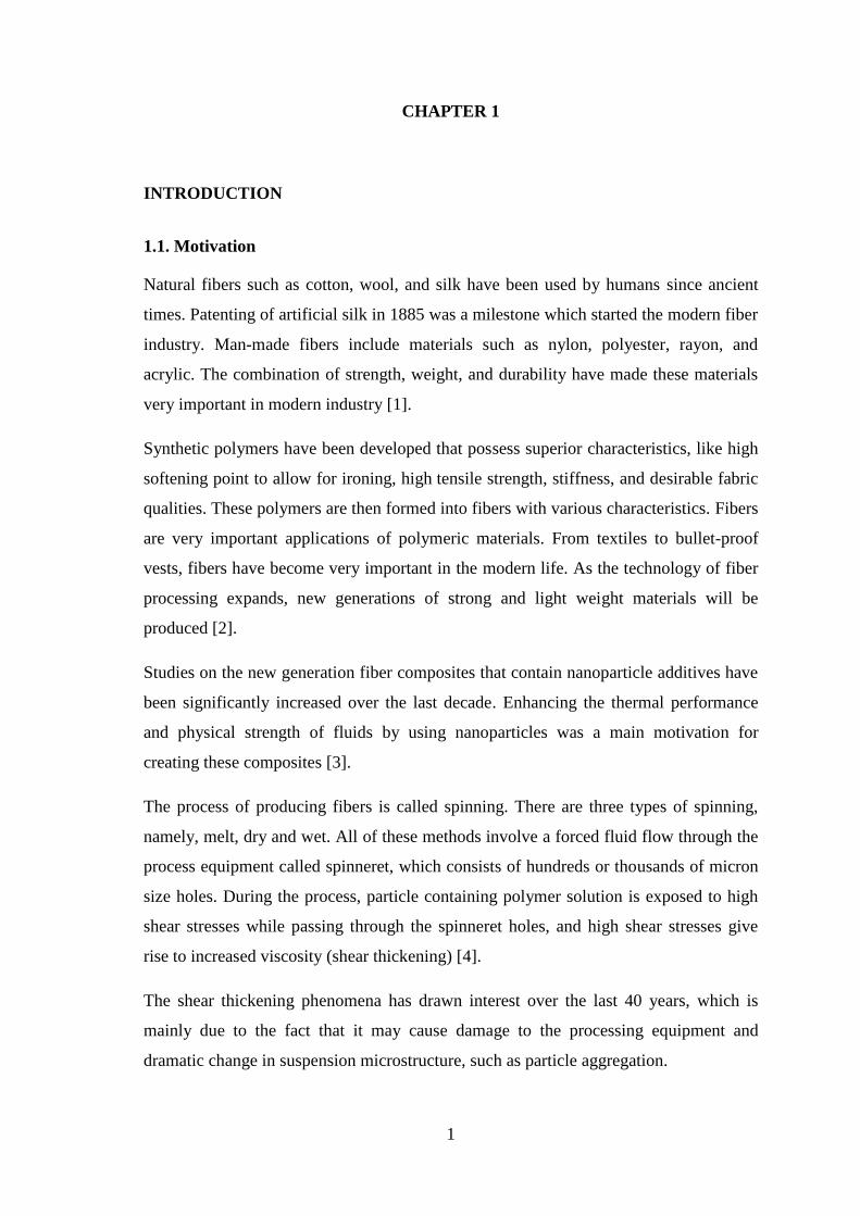
The process of producing fibers is called spinning. There are three types of spinning,
namely, melt, dry and wet. All of these methods involve a forced fluid flow through the
process equipment called spinneret, which consists of hundreds or thousands of micron
size holes. During the process, particle containing polymer solution is exposed to high
shear stresses while passing through the spinneret holes, and high shear stresses give
rise to increased viscosity (shear thickening) [4].
The shear thickening phenomena has drawn interest over the last 40 years, which is
mainly due to the fact that it may cause damage to the processing equipment and
dramatic change in suspension microstructure, such as particle aggregation.
2
For an industrial manufacturing process, it is crucial to maintain continuous production
without losing quality of the product. Yet, it is known that nanoparticle containing
fluids imperils the fiber production process by harming the process equipments,
clogging or narrowing micro channels, due to the shear thickening, arisen from the
particle aggregation and coagulation. This causes an enormous and intolerable loss of
time and money for companies; therefore, addressing this problem remains as of great
importance. CFD aided studies for investigating various types of multiphase fluid flow
problems in close conduits and open channels have been increasingly used because of
the advantages that they provide like rapid evaluation of multiphase flow problems
under a wide range of conditions, which is almost impossible experimentally [5-7].
In light of the above discussion, the motivation behind this study is to investigate and
understand the processing parameters which promote shear thickening inside the
channels of die. To this end, in this study, we have numerically scrutinized the effects of
die geometry and velocity on the flow behavior of shear thickening fluids.
1.2. Outline of the Thesis
The rest of this thesis continues as follows. Section 2 briefly provides some information
about the basics of rheology, and CFD method for multiphase fluid flows. Shear
thickening phenomenon as well as some relevant studies dedicated to explain this
phenomenon are discussed in Section 2. In this section, a number of pertinent CFD
studies are also cited and briefly summarized. In section 3, the governing equations and
constitutive relations used to numerically model the problem in question are provided in
detail. Geometry, mesh, material properties and numerical methods are described in
Section 4. Results of the numerical study are discussed in Section 5. The present work is
concluded with final remarks and the future work in Section 6.
3
CHAPTER 2
BACKGROUND
2.1. Rheology Basics
Fluids having direct proportionality between shear stress (𝜍) and shear rate (𝛾 ) under a
simple shear are called as “Newtonian Fluids”. The behavior of these types of fluids are
expressed by a relation of the form given in equation (1) where 𝜇 is the viscosity, which
does not depend on the shear rate but might depend on the external factors like
temperature and pressure. Most low-molecular-weight materials like organic and
inorganic liquids, molten metals and gases exhibit Newtonian behavior under a simple
shear [8].
𝜍𝑥𝑦 = 𝜇 ∗ 𝛾 ,
(1)
Fluids with non-proportional relationship between shear stress and shear rate are
referred to non-Newtonian fluids. Shear rate dependent viscosity is one of the most
important characteristic features of these fluids, where viscosity is time-independent but
depends on the type and rate of deformation. These fluids can be either shear-thinning
(pseudo-plastic), where viscosity decreases with increasing shear rate or shear-
thickening (dilatant) where viscosity increases with increasing shear rate. Fluids
exhibiting a combination of shear thinning and shear thickening behavior are so-called
complex fluids [9].
Shear thinning and shear thickening fluids have been intensely studied and investigated
by both academy and industry over the last few decades. Shear thinning is the most
widely encountered type of time-independent non-Newtonian fluid behavior in
engineering practice and the physics behind shear thinning is far more established
compared to shear thickening. [10]
Shear thickening fluids can have supreme applications like shock absorbing and force
damping skis, tennis rackets and flexible body armor when they are engineered into
composite materials, but yet they may harm the process equipments by clogging the
pipes or spraying equipments. Many colloidal suspensions, such as dies, paints,
4
coatings, and lubricants, are subjected to high shear rates during processing. Sometimes,
shear rate is high enough to drive shear thickening, which means viscosity increases
discontinuously with small increases in shear rate. This behavior can damage processing
equipment and provoke changes in the suspension microstructure such as driving
irreversible flocculation and particle aggregation [11, 12].
Many theories have been suggested in the literature in order to explain the origin of the
shear thickening phenomena. In the early 1970s, Hoffman claimed that, shear
thickening is a consequence of an order-to-disorder transition (ODT) of the fluid. Below
a certain shear rate, a colloidal fluid is ordered into layers, and with the applied shear,
this layered arrangement prevents collisions of colloidal particles and thus reduces
viscosity. Above the critical shear rate, the layered arrangement is disrupted by intense
hydrodynamic forces. As a consequence, increased collisions give rise to the
dramatically elevated viscosity. Hoffman confirmed this theory with his light-scattering
experiments [13].
Even though the ODT theory was well accepted and the study pioneered the curiosity
towards the shear thickening, thereafter, many studies have been done in this field in
order to further understand the physics behind the shear thickening phenomena. In a
review article that Barnes published in 1989, the author claimed that shear thickening
occurs in all dispersion systems, but this thickening is too marginal in some dispersions
to be detected with conventional rheometers. Nevertheless, shear thickening in some
dispersions is so severe and hence can easily be detected with rheometers. According to
Barnes, the parameters affecting shear thickening are: particle size, particle size
distribution, particle shape, particle volume fraction, particle-particle interaction,
continuous phase viscosity, and the type, rate and time of deformation. All of these
parameters have been studied in the literature so far [14, 15].
Some of the studies claimed that order-disorder transition is not necessary for shear
thickening. They claimed that suspensions that had a disordered arrangement of
particles at the very beginning, and even suspensions that contain only 2 particles which
have Brownian motion, may show shear thickening [11].
The non-Newtonian rheological behavior, e.g., shear thickening and/or shear thinning,
can be captured using simple equations relating viscosity and shear rate via minimum
number of parameters. Some of these equations are namely, the Carreau Model, the
5
Cross Model, the Power-Law Model and the Herschel-Bulkley Model. All of those
models are capable of capturing the fluid as either shear thickening or shear thinning
fluid. However, some non-Newtonian fluids show divergent behavior between shear
thickening and shear thinning. These so-called complex fluids, act as shear thinning
fluids below a certain shear rate, and above that shear rate they act as shear thickening
fluids. There is no model reported in the literature that is able to capture the complex
viscosity behavior [16, 17]. It is of great importance to handle the viscosity profile of a
fluid of interest, accurately. Accordingly, the lack of the constitutive equations
regarding the complex fluids leaves a challenge behind. In the present study, this
challenge has been attempted to be addressed.
2.2. Computational Fluid Dynamics for Multiphase Fluid Flows
In the field of polymeric materials, computers have been intensively used for industrial
and research applications. In particular, computational fluid dynamics (CFD) of
polymeric fluids has received growing attention for understanding the physics of
processes, thereby making it possible to design better equipments and optimize the
processing conditions [18].
The foundation of the CFD software are based on the principles of fluid mechanics,
together with improved numerical methods for the solution of the governing equations
and constitutive relations, which describe the rheological behavior of fluid and particles
if involved [18].
Most of the flow problems encountered in industrial processes involve complex
kinematics due to different geometries, combined shear and elongation, different time
dependences and amplitudes of deformations [18]. The physical phenomena of a
problem considered in this thesis work, are governed by partial differential equations,
which are rather complex for having analytical solutions, and hence need to be
discretized numerically. Numerical discretization is transformation of the partial
differential equations into linear sets of equations which can then be solved by using
appropriate numerical methods via computer programming. There are three main mesh
based numerical discretization techniques, namely, finite difference method, finite
element method and finite volume method [7, 19]. In this study, FLUENT software of
ANSYS Workbench is used and FLUENT uses the finite volume method for
discretization of partial differential equations.
6
CFD aided studies for investigating various types of multiphase fluid flow problems in
close conduits and open channels have been increasingly used. Main advantage of CFD
aided studies is that three dimensional solid–liquid two phase flow problems under a
wide range of flow conditions may be evaluated rapidly, which is almost impossible
experimentally. Particle processing, conveying and separation are of crucial importance
in industrial processes. Besides empirical correlations and experimental investigations,
numerical simulations have gained significant attention in studying particle containing
flows. There are quite much of studies in the literature involving the particle containing
flows [7].
In computational simulations, regardless of the method being used for handling the
problem of particulate fluid flow, it is mandatory to cover the dominant flow regimes of
the process accurately. For instance, Ristic et al. simulated the multiphase flow in
ventilation mill, ventilation channel and centrifugal separator. They started to simulate
the flow by using Eulerian-Eulerian approach and showed that their numerical model
did not show any convergent behavior because of the complex geometry and large
number of grids. Then they have used the mixture model and the Eulerian-Lagrangian
approach, and obtained results which are in good agreement with the experimental
results. Their study also showed the importance of using the right approach for handling
the flow problem [20, 21].
Employing a specific multiphase model (the discrete phase, mixture, Eulerian model) to
handle the momentum transfer depends on the volume fraction of solid particles and on
the fulfillment of the requirements, which enable the selection of a given model. The
problem that we investigate is a diluted system. Therefore the discrete phase model, the
mixture model and the Eulerian model are appropriate in this case. The Eulerian model
has two versions, namely granular version and the non-granular version. Granular
version is preferable in our case since non-granular version does not include models for
handling friction and collisions between particles into account which is believed to be of
importance in nanoparticulate fluids [22].
Most of the studies, regarding to the nanoparticle containing multiphase flows found in
the literature, have dealt with the heat transfer properties of the flows by using CFD
methods. Abbassi et al. modeled forced convection of laminar nanofluids flowing
trough microchannels by using Eulerian-Eulerian multiphase model and FLUENT
7
software. They investigated the influence of concentration and size nanoparticles on the
Nusselt number and pressure drop [23]. Kamali and Binesh numerically investigated
multi-wall carbon nanotube (MWCNT) based nanofluids in a straight tube under
constant heat flux condition. They simulated the nanofluid flow passing through the
tube by using in-house built numerical code, with the non-Newtonian power-law fluid
model and found that the heat transfer coefficient is dominated by the wall region due to
non-Newtonian behavior of nanofluid. [24]. Apart from these, one may find quite many
studies in the literature, which have focused on the heat transfer properties of
nanoparticulate multiphase flows [25-27].
One may find immense many numbers of experimental studies devoted to understand
the physics behind the shear thickening phenomena, and the various parameters
affecting shear thickening. However, there are a limited number of computational
studies in the literature which have focused on the rheological behavior of shear
thickening fluids. Out of these computational studies, the majority of the works
investigated the heat transfer properties of these fluids or some other properties, and
only a few of them computationally investigated the parameters affecting shear
thickening, which are of significant importance in fiber spinning processes. This study
aims to understand parameters, namely geometry and fluid velocity which potentially
affect the shear thickening behavior inside the spinneret in fiber spinning processes.
Barigou et al. studied viscous non-Newtonian flow under the influence of a
superimposed rotational vibration by employing different fluids of the power-law,
Hershel-Bulkley and Bingham plastic types [28]. Chabbra et al. investigated
numerically two-dimensional laminar flow of power-law fluids past a long square
cylinder confined in a planar channel for various Reynolds numbers and blockage
ratios. They presented extensive numerical results, to elucidate the effects of blockage,
power-law index and Reynolds number on the drag coefficient, stream function,
vorticity etc. [29]. Shah and Manzar studied particle conveying Newtonian and non-
Newtonian slurries in straight and coiled pipes by using CFD and showed in their
studies that shear stress inside the flow domain, increases with increasing values of flow
rate, particle size, particle density and particle loading. They also found that there is a
good agreement between near-wall particle concentration and particle shear stress [30].
8
Non-newtonian fluids have a wide variety of applications in the food industry as well.
The shear rheology of bread dough was studied by Hicks et al. The geometry consisted
a sudden contraction where shear rate increased significantly, resulting in increased
viscosity. Their results showed that shear rate and viscosity tend to be higher nearby the
walls and contraction areas, and this increase in shear rate and viscosity tends to be
more tremendous with higher flow rates [31]. Sun and Norton reviewed numerous
articles and showed the importance of CFD methods for studying thermal and hydraulic
performance of non-Newtonian fluids in food industry like milk, yogurt, soup etc. [32].
9
CHAPTER 3
FORMULATION OF CFD MODEL
The Eulerian-Eulerian two fluid model was used in the computational studies described
within this thesis.
The Eulerian-Eulerian multiphase model assumes that the flow consists of solid “s” and
fluid “f” phases, that are separate yet they form interpenetrating continua, so that
𝛼𝑓 + 𝛼𝑠 = 1, here 𝛼𝑓 and 𝛼𝑠 are the volumetric concentrations of fluid and solid phases,
respectively. The Eulerian-Eulerian model solves two sets of momentum and continuity
equations for each phase. Coupling between phases is achieved through the pressure and
interphase exchange coefficients. [33]
The laminar flow of non-Newtonian fluid containing nanoparticles is assumed to be
governed by the following equations, which form the basis of the Eulerian-Eulerian
CFD model used.
3.1. Conservation of Mass
The continuity equation for phase q is:
1
𝜌𝑟𝑞 𝜕
𝜕𝑡 𝛼𝑞𝜌𝑞 + 𝛻 · 𝛼𝑞𝜌𝑞𝑣 𝑞 = (ṁ𝑝𝑞 −ṁ𝑞𝑝 )
𝑛
𝑝=1
,
(2)
where 𝑣 𝑞 is the velocity of phase q and 𝑚 q characterizes the mass transfer between pth
and qth
phase, and 𝑚 pq characterizes the mass transfer from phase q to phase p, and it is
possible to specify these mechanisms, separately.
3.2. Conservation of Momentum
The general form of momentum balance for phase q is:
𝜕
𝜕𝑡 𝛼𝑞𝜌𝑞𝑣 𝑞 + 𝛻 · 𝛼𝑞𝜌𝑞𝑣 𝑞𝑣 𝑞 = −𝛼𝑞𝛻𝑝 + 𝛻 · 𝜏 𝑞 + 𝛼𝑞𝜌𝑞𝑔 +
𝑅 𝑝𝑞 +ṁ𝑝𝑞 𝑣 𝑝𝑞 −ṁ𝑞𝑝𝑣 𝑞𝑝 + 𝐹 𝑞 + 𝐹 𝑙𝑖𝑓𝑡 ,𝑞 + 𝐹 𝑣𝑚 ,𝑞 ,
𝑛
𝑝=1
(3)
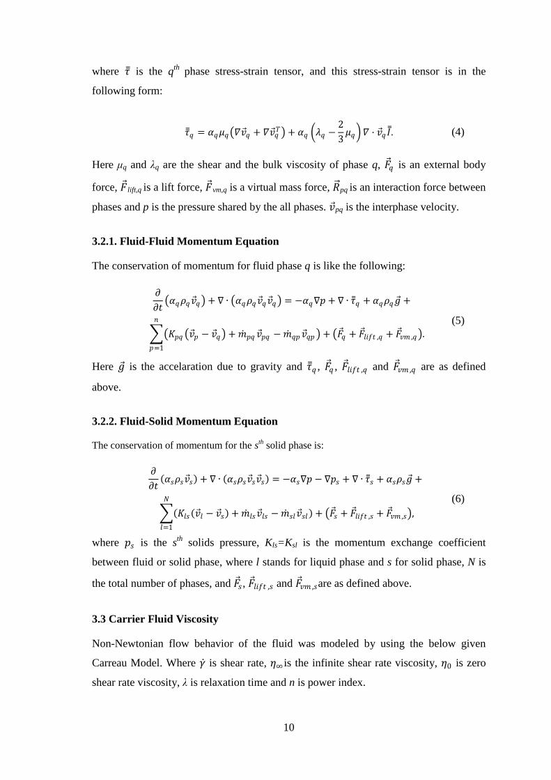
10
where 𝜏 is the qth
phase stress-strain tensor, and this stress-strain tensor is in the
following form:
𝜏 𝑞 = 𝛼𝑞𝜇𝑞 𝛻𝑣 𝑞 + 𝛻𝑣 𝑞𝑇 + 𝛼𝑞 𝜆𝑞 −
2
3𝜇𝑞 𝛻 · 𝑣 𝑞𝐼 .
(4)
Here μq and λq are the shear and the bulk viscosity of phase q, 𝐹 𝑞 is an external body
force, 𝐹 lift,q is a lift force, 𝐹 vm,q is a virtual mass force, 𝑅 pq is an interaction force between
phases and p is the pressure shared by the all phases. 𝑣 pq is the interphase velocity.
3.2.1. Fluid-Fluid Momentum Equation
The conservation of momentum for fluid phase q is like the following:
𝜕
𝜕𝑡 𝛼𝑞𝜌𝑞𝑣 𝑞 + ∇ ∙ 𝛼𝑞𝜌𝑞𝑣 𝑞𝑣 𝑞 = −𝛼𝑞∇𝑝 + ∇ ∙ 𝜏 𝑞 + 𝛼𝑞𝜌𝑞𝑔 +
𝐾𝑝𝑞 𝑣 𝑝 − 𝑣 𝑞 +𝑚 𝑝𝑞 𝑣 𝑝𝑞 −𝑚 𝑞𝑝𝑣 𝑞𝑝 + 𝐹 𝑞 + 𝐹 𝑙𝑖𝑓𝑡 ,𝑞 + 𝐹 𝑣𝑚 ,𝑞
𝑛
𝑝=1
.
(5)
Here 𝑔 is the accelaration due to gravity and 𝜏 𝑞 , 𝐹 𝑞 , 𝐹 𝑙𝑖𝑓𝑡 ,𝑞 and 𝐹 𝑣𝑚 ,𝑞 are as defined
above.
3.2.2. Fluid-Solid Momentum Equation
The conservation of momentum for the sth solid phase is:
𝜕
𝜕𝑡 𝛼𝑠𝜌𝑠𝑣 𝑠 + ∇ ∙ 𝛼𝑠𝜌𝑠𝑣 𝑠𝑣 𝑠 = −𝛼𝑠∇𝑝 − ∇𝑝𝑠 + ∇ ∙ 𝜏 𝑠 + 𝛼𝑠𝜌𝑠𝑔 +
𝐾𝑙𝑠 𝑣 𝑙 − 𝑣 𝑠 +𝑚 𝑙𝑠𝑣 𝑙𝑠 −𝑚 𝑠𝑙𝑣 𝑠𝑙 + 𝐹 𝑠 + 𝐹 𝑙𝑖𝑓𝑡 ,𝑠 + 𝐹 𝑣𝑚 ,𝑠 ,
𝑁
𝑙=1
(6)
where 𝑝𝑠 is the sth
solids pressure, Kls=Ksl is the momentum exchange coefficient
between fluid or solid phase, where l stands for liquid phase and s for solid phase, N is
the total number of phases, and 𝐹 𝑠, 𝐹 𝑙𝑖𝑓𝑡 ,𝑠 and 𝐹 𝑣𝑚 ,𝑠are as defined above.
3.3 Carrier Fluid Viscosity
Non-Newtonian flow behavior of the fluid was modeled by using the below given
Carreau Model. Where 𝛾 is shear rate, 𝜂∞ is the infinite shear rate viscosity, 𝜂0 is zero
shear rate viscosity, λ is relaxation time and n is power index.
11
𝜂 = 𝜂∞ + 𝜂0 − 𝜂∞ 1 + 𝛾 2𝜆2 𝑛−1 2 . (7)
3.4. The Pressure Correction Equation
For incompressible multiphase flow, the pressure-correction equation is in the following
form:
1
𝜌𝑟𝑘 𝜕
𝜕𝑡𝛼𝑘𝜌𝑘 + ∇ ∙ 𝛼𝑘𝜌𝑘𝑣 𝑘
′ + ∇ ∙ 𝛼𝑘𝜌𝑘𝑣 𝑘∗ − 𝑚 𝑙𝑘 −𝑚 𝑘𝑙
𝑛
𝑙=1
= 0,
𝑛
𝑘=1
(8)
where 𝜌𝑟𝑘 is the phase reference density for the kth
phase (defined as the total volume
average density of phase k), 𝑣 𝑘′ is the velocity correction for the k
th phase, and 𝑣 𝑘
∗ is the
value of 𝑣 𝑘 at the current iteration. The velocity corrections are expressed as functions
of the pressure corrections.
3.5. Volume Fraction Equation
The description of multiphase flow incorporates the concept of phasic volume fractions,
denoted here by αq. Volume fractions represent the space occupied by each phase, and
the laws of conservation of mass and momentum are satisfied by each phase
individually [33].
The volume of phase q, Vq, is defined by:
𝑉𝑞 = 𝛼𝑞𝑉
𝑑𝑉,
(9)
where
𝛼𝑞 = 1.
𝑛
𝑞=1
(10)
The effective density of phase q is 𝜌 q = αq ρq where ρq is the physical density of phase q.
3.6. Fluid-Solid Exchange Coefficient
Within particulate fluid flows, fluid-solid exchange can be described by using many
models which were developed empirically, like Gidaspow [34], Syamlal-O’Brian [35],
Huilin-Gidaspow [36], Gibilaro [37], and Wen-Yu models. The model developed by
Wen and Yu was used in our study, since it is the best choice for systems involving
particles less than twenty percent. For the model of Wen-Yu, the fluid-solid exchange
coefficient is of the following form:
12
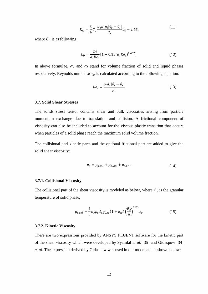
𝐾𝑠𝑙 =3
4𝐶𝐷𝛼𝑠𝛼𝑙𝜌𝑙 𝑣 𝑠 − 𝑣 𝑙
𝑑𝑠𝛼𝑙 − 2.65,
(11)
where 𝐶𝐷 is as following:
𝐶𝐷 =24
𝛼𝑙𝑅𝑒𝑠 1 + 0.15 𝛼𝑙𝑅𝑒𝑠
0.687 .
(12)
In above formulae, 𝛼𝑠 and 𝛼𝑙 stand for volume fraction of solid and liquid phases
respectively. Reynolds number,𝑅𝑒𝑠, is calculated according to the following equation:
𝑅𝑒𝑠 =𝜌𝑙𝑑𝑠 𝑣 𝑠 − 𝑣 𝑠
𝜇𝑙. (13)
3.7. Solid Shear Stresses
The solids stress tensor contains shear and bulk viscosities arising from particle
momentum exchange due to translation and collision. A frictional component of
viscosity can also be included to account for the viscous-plastic transition that occurs
when particles of a solid phase reach the maximum solid volume fraction.
The collisional and kinetic parts and the optional frictional part are added to give the
solid shear viscosity:
𝜇𝑠 = 𝜇𝑠,𝑐𝑜𝑙 + 𝜇𝑠,𝑘𝑖𝑛 + 𝜇𝑠,𝑓𝑟 .. (14)
3.7.1. Collisional Viscosity
The collisional part of the shear viscosity is modeled as below, where Θ𝑠 is the granular
temperature of solid phase.
𝜇𝑠,𝑐𝑜𝑙 =4
5𝛼𝑠𝜌𝑠𝑑𝑠𝑔0,𝑠𝑠 1 + 𝑒𝑠𝑠
Θ𝑠π
1 2
𝛼𝑠 . (15)
3.7.2. Kinetic Viscosity
There are two expressions provided by ANSYS FLUENT software for the kinetic part
of the shear viscosity which were developed by Syamlal et al. [35] and Gidaspow [34]
et al. The expression derived by Gidaspow was used in our model and is shown below:
13
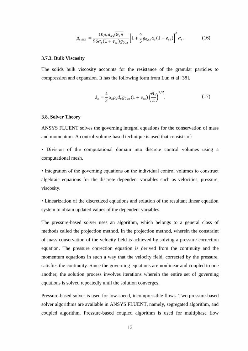
𝜇𝑠,𝑘𝑖𝑛 =10𝜌𝑠𝑑𝑠 Θ𝑠𝜋
96𝛼𝑠 1 + 𝑒𝑠𝑠 𝑔0,𝑠𝑠 1 +
4
5𝑔0,𝑠𝑠𝛼𝑠 1 + 𝑒𝑠𝑠
2
𝛼𝑠 .
(16)
3.7.3. Bulk Viscosity
The solids bulk viscosity accounts for the resistance of the granular particles to
compression and expansion. It has the following form from Lun et al [38].
𝜆𝑠 =4
3𝛼𝑠𝜌𝑠𝑑𝑠𝑔0,𝑠𝑠 1 + 𝑒𝑠𝑠
Θ𝑠𝜋
1 2
.
(17)
3.8. Solver Theory
ANSYS FLUENT solves the governing integral equations for the conservation of mass
and momentum. A control-volume-based technique is used that consists of:
• Division of the computational domain into discrete control volumes using a
computational mesh.
• Integration of the governing equations on the individual control volumes to construct
algebraic equations for the discrete dependent variables such as velocities, pressure,
viscosity.
• Linearization of the discretized equations and solution of the resultant linear equation
system to obtain updated values of the dependent variables.
The pressure-based solver uses an algorithm, which belongs to a general class of
methods called the projection method. In the projection method, wherein the constraint
of mass conservation of the velocity field is achieved by solving a pressure correction
equation. The pressure correction equation is derived from the continuity and the
momentum equations in such a way that the velocity field, corrected by the pressure,
satisfies the continuity. Since the governing equations are nonlinear and coupled to one
another, the solution process involves iterations wherein the entire set of governing
equations is solved repeatedly until the solution converges.
Pressure-based solver is used for low-speed, incompressible flows. Two pressure-based
solver algorithms are available in ANSYS FLUENT, namely, segregated algorithm, and
coupled algorithm. Pressure-based coupled algorithm is used for multiphase flow
14
problems. The pressure-based coupled algorithm solves a coupled system of equations
comprising the momentum equations and the pressure-based continuity equation. With
the coupled algorithm, each iteration consists of the steps as outlined below:
1. Update fluid properties (e.g., density, viscosity) based on the current solution.
2. Solve the coupled system of momentum and pressure correction equations, using the
recently updated values of pressure, mass flux and velocity field.
3. Correct mass fluxes using the pressure correction obtained from Step 2.
4. Solve the equations for additional scalars, if any, using the current values of the
solution variables.
5. Update the source terms arising from the interactions between different phases (e.g.,
source term for the carrier phase due to discrete particles).
6. Check for the convergence of the equations.
Since the momentum and continuity equations are solved in a closely coupled manner,
the rate of solution convergence significantly improves compared to the segregated
algorithm. However, the memory requirement increases by 1.5 – 2 times that of the
segregated algorithm since the discrete system of all momentum and pressure-based
continuity equations needs to be stored in the memory when solving for the velocity and
pressure fields.
15
CHAPTER 4
DESCRIPTION OF CFD SIMULATIONS
All of the simulations described within this thesis were performed by using ANSYS
Workbench Release 14.0 and solved by using the FLUENT solver component of the
package.
4.1. Simulation of Validation Case
In order to check the validity and the accuracy of the solver, a reference study by Ease
and Barigou has been considered where the numerical modeling of a flow through
channels were conducted with the assumptions of 2D, incompressible, isothermal, and
fully developed flow. The test case modeled in this work as a validation is a flow
through a straight pipe with the diameter and length of 45 mm, and 600 mm,
respectively. The geometry was meshed with in total 32000 fine cells. A non-
Newtonian power law fluid model given in Equation (18) was used with the consistency
index, k, of 0.16 Pa.sn and power-law index, n, of 0.81. The density of the fluid is 1000
kg/m3. Velocity inlet boundary condition was used at the inlet with the value of inlet
velocity of 0.066 m/s while the zero gauge pressure condition was used at the outlet.
Walls were considered to have no-slip boundary conditions.
𝜂 = 𝑘𝛾 𝑛−1, (18)
Initially, the fluid without any particles was modeled and the results were compared
with the analytical ones. Governing equations were discretized using SIMPLE
algorithm and momentum equation was dicretized using second-order upwind
differencing scheme. Residual target was 10-5
and convergence was reached after
approximately 800 iterations at steady state conditions.
The shear thickening fluid containing 30% v/v particles with diameter of 2mm was
modeled and the particle velocity results were compared with the ones in the reference
paper. Governing equations were discretized using phase coupled SIMPLE algorithm
and momentum equation was dicretized using second-order upwind differencing
scheme. Residual target was 10-4
and convergence was reached after approximately 130
time steps, with 10 iterations at each time step, and with a small time step size as 0.05.
16
4.2. Simulations of Single Phase Fluid Flow and Two-Phase Solid-Liquid Flow
4.2.1. Geometry
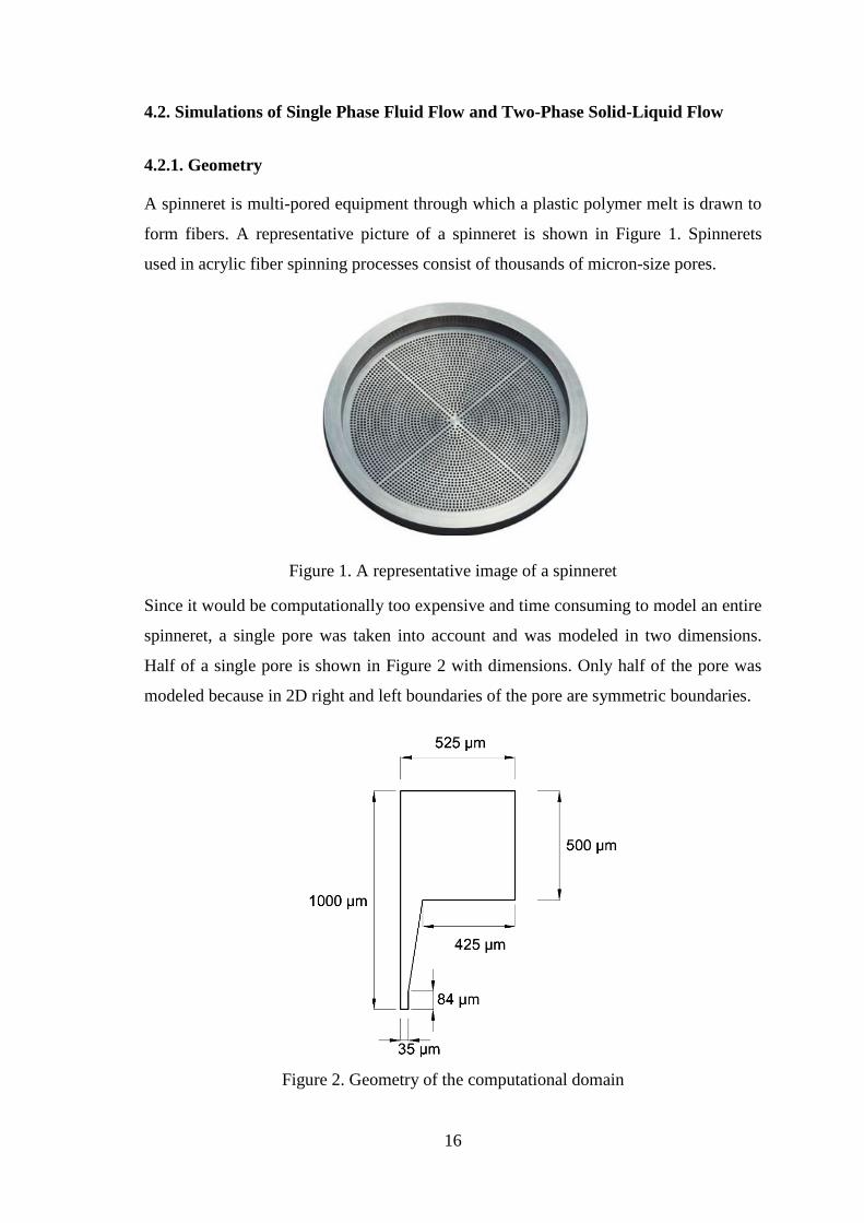
A spinneret is multi-pored equipment through which a plastic polymer melt is drawn to
form fibers. A representative picture of a spinneret is shown in Figure 1. Spinnerets
used in acrylic fiber spinning processes consist of thousands of micron-size pores.
Figure 1. A representative image of a spinneret
Since it would be computationally too expensive and time consuming to model an entire
spinneret, a single pore was taken into account and was modeled in two dimensions.
Half of a single pore is shown in Figure 2 with dimensions. Only half of the pore was
modeled because in 2D right and left boundaries of the pore are symmetric boundaries.
Figure 2. Geometry of the computational domain
17
4.2.2. Mesh
For two dimensional channel flows, it is recommended to mesh the computational
domain with tetrahedral elements. Therefore, the mesh was generated with 9791
tetrahedral elements. The quality of the mesh was 0.9 on a scale from 0 to 1, where 0
and 1 correspond to the lowest and highest quality, respectively.
4.2.3. Material Properties
In the context of this work, it was aimed to investigate the flow behavior of shear-
thickening fluids, flowing through tiny spinneret holes. The shear-thickening fluid
which was used in simulations was prepared in-house instead of taking an example from
the literature. As explained in the second section of this thesis, neat fluids do not show
shear thickening. Therefore, nanoparticle embedded shear thickening fluid was
prepared.
Yıldız et al. showed in their recent paper that silica nanoparticle containing
poly(ethyleneglycol) (PEG) solutions show complex rheological behavior [39]. In the
light of this study, silica-PEG system was prepared as a baseline fluid with the intention
of using the rheological data collected from this system in the simulations. Silica
nanoparticles, which were 400 nm in diameter, were dispersed in PEG, molecular
weight of 200, by using shear mixer at 1000 rpm for 3 hours. Rheology measurements
were conducted afterwards on this sample by using Malvern Bohlin 2000 rheometer.
Sample first showed shear thinning at lower shear rates, and then it started to thicken
after a certain threshold.
As discussed in Section 2, non-Newtonian fluids can be modeled by using several
models like power-law, Carreau and Cross model. However, none of these models are
capable of expressing the complex viscosity profile (both shear thinning and
thickening). Therefore, a model was needed to introduce the viscosity of a complex
fluid to the FLUENT. This was achieved by an in-house developed User Defined
Function (UDF). The UDF simply defined the viscosity in two parts. If the shear rate is
below the threshold, shear thinning part of the UDF was used by the software, and if the
shear rate is above the threshold, shear thickening part of the UDF was used.
Viscosity profile obtained from the rheometer was first splitted into two as shear
thinning and shear thickening parts. Afterwards these two parts were curve fitted to the
18
Carreau Fluid Model which is given in Equation (19) separately by using the Solver
module of MS Office Excel. By using the data from the curve fittings, the UDF was
developed and the viscosity was introduced to the FLUENT by using it. Carreau model
parameters are given in Table 1. The real viscosity profile obtained from the rheometer
and curve fitted one are shown in Figure 3. The compatibility of these two curves
indicates that Carreau model formed of two parts is a good representative for our fluid
sample.
𝜇 = 𝜇∞ + 𝜇0 − 𝜇∞ 1 + 𝛾 2𝜆2 𝑛−1 2 . (19)
Table 1. Carreau Model Parameters
Carreau Model Parameters Shear Thinning Part Shear Thickening Part
𝜇∞ 0 0
𝜇0 9,197351 1,873088
𝜆 20,61487 0,021371
𝑛 0,75726 26,67904
Figure 3. Viscosity profile of the fluid used in simulations as a function of shear rate,
and its curve fitting to the Carreau Model
4.2.4. Description of the Numerical Model
As discussed in previous sections, nanoparticles were introduced in the continuous
liquid phase as a second Eulerian phase.
10-2
10-1
100
101
102
103
104
0.2
0.3
0.4
0.5
0.6
0.7
0.8
0.9
1
Shear Rate (1/s)
Vis
cosity (
Pa.s
)
Carreau model, Predicted viscosity
Real Viscosity
19
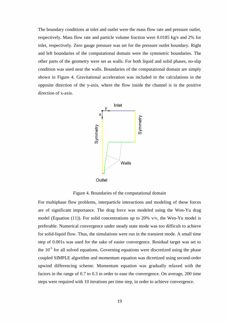
The boundary conditions at inlet and outlet were the mass flow rate and pressure outlet,
respectively. Mass flow rate and particle volume fraction were 0.0185 kg/s and 2% for
inlet, respectively. Zero gauge pressure was set for the pressure outlet boundary. Right
and left boundaries of the computational domain were the symmetric boundaries. The
other parts of the geometry were set as walls. For both liquid and solid phases, no-slip
condition was used near the walls. Boundaries of the computational domain are simply
shown in Figure 4. Gravitational acceleration was included in the calculations in the
opposite direction of the y-axis, where the flow inside the channel is in the positive
direction of x-axis.
Figure 4. Boundaries of the computational domain
For multiphase flow problems, interparticle interactions and modeling of these forces
are of significant importance. The drag force was modeled using the Wen-Yu drag
model (Equation (11)). For solid concentrations up to 20% v/v, the Wen-Yu model is
preferable. Numerical convergence under steady state mode was too difficult to achieve
for solid-liquid flow. Thus, the simulations were run in the transient mode. A small time
step of 0.001s was used for the sake of easier convergence. Residual target was set to
the 10-5
for all solved equations. Governing equations were discretized using the phase
coupled SIMPLE algorithm and momentum equation was dicretized using second-order
upwind differencing scheme. Momentum equation was gradually relaxed with the
factors in the range of 0.7 to 0.3 in order to ease the convergence. On average, 200 time
steps were required with 10 iterations per time step, in order to achieve convergence.
20
CHAPTER 5
RESULTS AND DISCUSSION
5.1. Validation Case
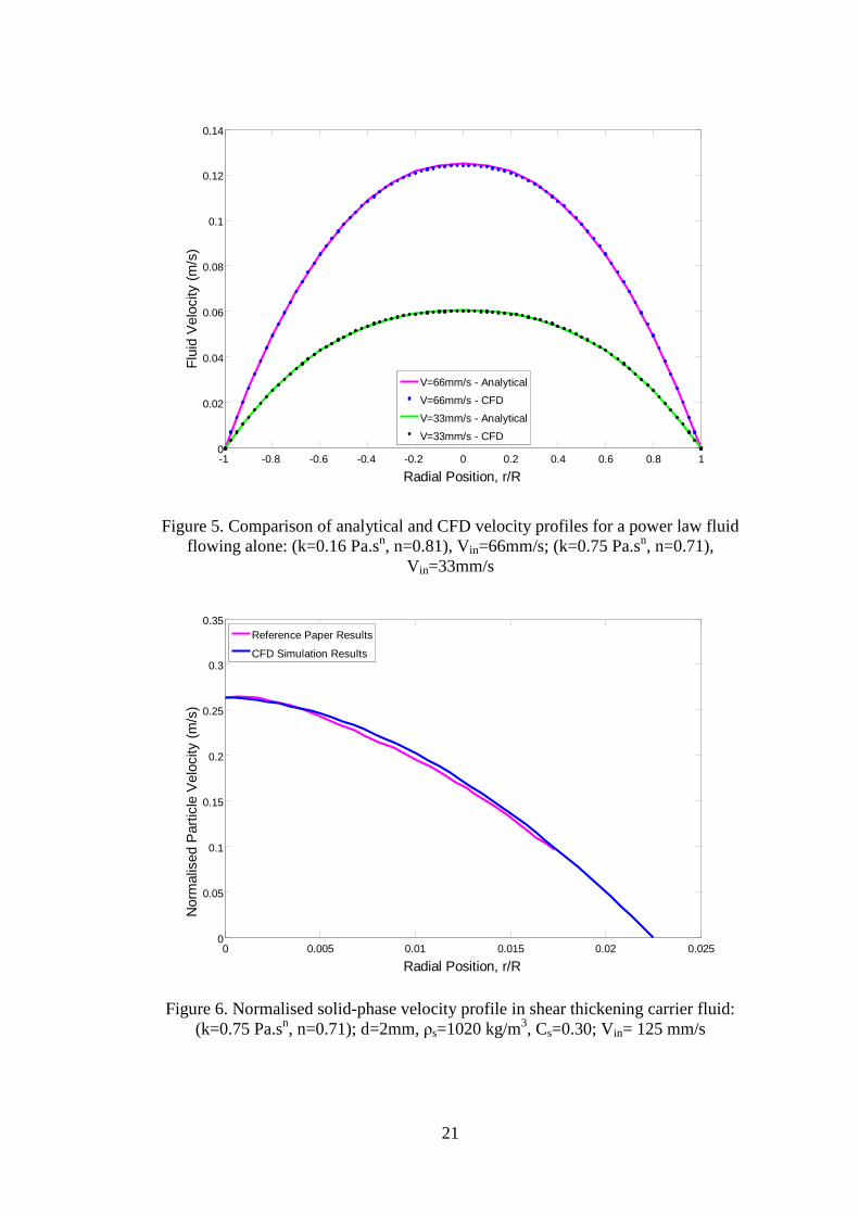
In order to ensure the validation and reliability of the commercial code, the study of
Ease and Barigou [40] was taken as a reference. The results were duplicated and they
were compared with the analytical results obtained by using equations (20) and (21)
[41].
The volumetric flow rate, Q, of a power law fluid is given by the following equation
𝑄 =𝑛𝜋𝑅3
3𝑛 + 1 𝑅
2𝑘
𝛥𝑝
𝐿
1/𝑛
,
(20)
where R is the pipe radius, and ΔP/L is the pressure drop per unit length. The fluid
velocity profile can be derived by using the following relation where r is radial position.
𝑣 𝑟 =𝑛
𝑛 + 1 𝛥𝑝𝑅
2𝑘𝐿
1/𝑛
𝑅 1− 𝑟
𝑅 𝑛+1 /𝑛
.
(21)
All of the variables in Eq. (20) are known including, Q, n, k and R. By inserting all of
these known variables into the equation, pressure drop per unit length was calculated.
Then this calculated pressure drop were inserted into the Eq. (21), and by giving
different values to the r, velocities across the radius were analytically calculated. These
analytical results were compared to the ones that were obtained from the simulations
and the results are given in Figure 5.
Single phase flow simulations were performed for two different cases, where power-law
parameters and inlet velocity were changed. Analytical and CFD results for these two
cases were exactly the same as it is shown in Figure 5. This situation indicates that the
commercial CFD code that we used is capable of modeling non-Newtonian single phase
flows and the results obtained from the code are reliable. Multiphase flow simulations
were done for 30% v/v particle containin shear thickening fluid. The particle velocity
results are given in Figure 6, which are in excellent agreement with that given in the
reference paper of by Ease and Barigou [40]. These simulations confirmed the validity
and reliability of the commercial CFD code.
21
Figure 5. Comparison of analytical and CFD velocity profiles for a power law fluid
flowing alone: (k=0.16 Pa.sn, n=0.81), Vin=66mm/s; (k=0.75 Pa.s
n, n=0.71),
Vin=33mm/s
Figure 6. Normalised solid-phase velocity profile in shear thickening carrier fluid:
(k=0.75 Pa.sn, n=0.71); d=2mm, ρs=1020 kg/m
3, Cs=0.30; Vin= 125 mm/s
-1 -0.8 -0.6 -0.4 -0.2 0 0.2 0.4 0.6 0.8 10
0.02
0.04
0.06
0.08
0.1
0.12
0.14
Radial Position, r/R
Flu
id V
elo
city (
m/s
)
V=66mm/s - Analytical
V=66mm/s - CFD
V=33mm/s - Analytical
V=33mm/s - CFD
0 0.005 0.01 0.015 0.02 0.0250
0.05
0.1
0.15
0.2
0.25
0.3
0.35
Radial Position, r/R
Norm
alis
ed P
art
icle
Velo
city (
m/s
)
Reference Paper Results
CFD Simulation Results
22
5.2. Two-Phase Solid-Liquid Flow
5.2.1. Mesh Dependency Analysis
The mesh independence tests involve refining the initial mesh by increasing the number
of cells present in the initial mesh by approximately 1-3 folds. For the standard
geometry (case 1, details given in Table 2), mesh size of 2797 cells was first refined to
11188 cells and then to 25173 cells, for the entire geometry. There was no further
improvement found in simulations results, after the number of cells has been increased
from 2797 to 11188 and 25173. Therefore, optimum mesh was assumed to be the one
containing 2797 cells and it was computationally the most economical option. Same
mesh dependence study were also done on the altered geometries as well (cases 2 to 9,
details given in Table 2), and it was found that refinements didn’t change the
simulations results. Therefore, non-refined meshes were used for each case.
5.2.2. Parametric Study
Initial simulations were conducted on the standard geometry with a standard inlet
velocity and particle loading as described in section 3.2.1. Afterwards, changes were
made in the geometry in order to understand the effect of the geometry on the flow
behavior and viscosity of the fluid. Besides, it is known from the literature that fluid
and/or particle velocity also affects the shear rate and viscosity. Therefore, different
inlet velocities were used in simulations in order to observe their effects on the
viscosity.
5.2.2.1. Geometry
In order to investigate the effect of the geometry to the flow behavior of multiphase
fluid, various forms of the initial geometry were created by modifying certain sections
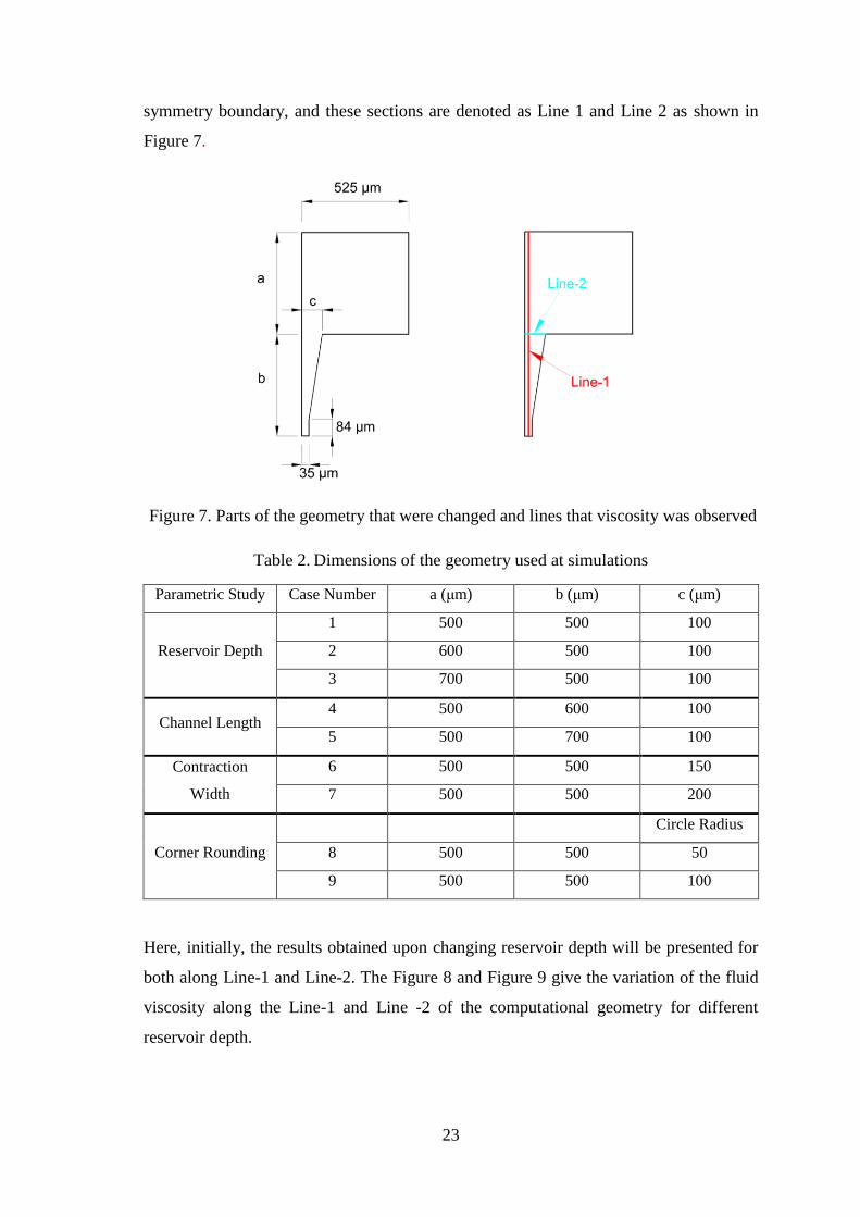
(denoted by the letters a, b and c) of the initial geometry as shown in Figure 7. In Table
2, parameters of these sections are shown in detail. Other sections of the geometry have
remained unchanged noting that there are some process induced constrains for the
spinneret geometry such as the hole sizes that controls the fiber diameter.
In order to see the relative change of viscosity more clearly compared to the zero shear
rate viscosity, viscosity profiles were normalized using the zero shear viscosity.
Viscosity profiles are shown across the contraction, and along the spinneret close to the
23
symmetry boundary, and these sections are denoted as Line 1 and Line 2 as shown in
Figure 7.
Figure 7. Parts of the geometry that were changed and lines that viscosity was observed
Table 2. Dimensions of the geometry used at simulations
Parametric Study Case Number a (μm) b (μm) c (μm)
Reservoir Depth
1 500 500 100
2 600 500 100
3 700 500 100
Channel Length 4 500 600 100
5 500 700 100
Contraction
Width
6 500 500 150
7 500 500 200
Corner Rounding
Circle Radius
8 500 500 50
9 500 500 100
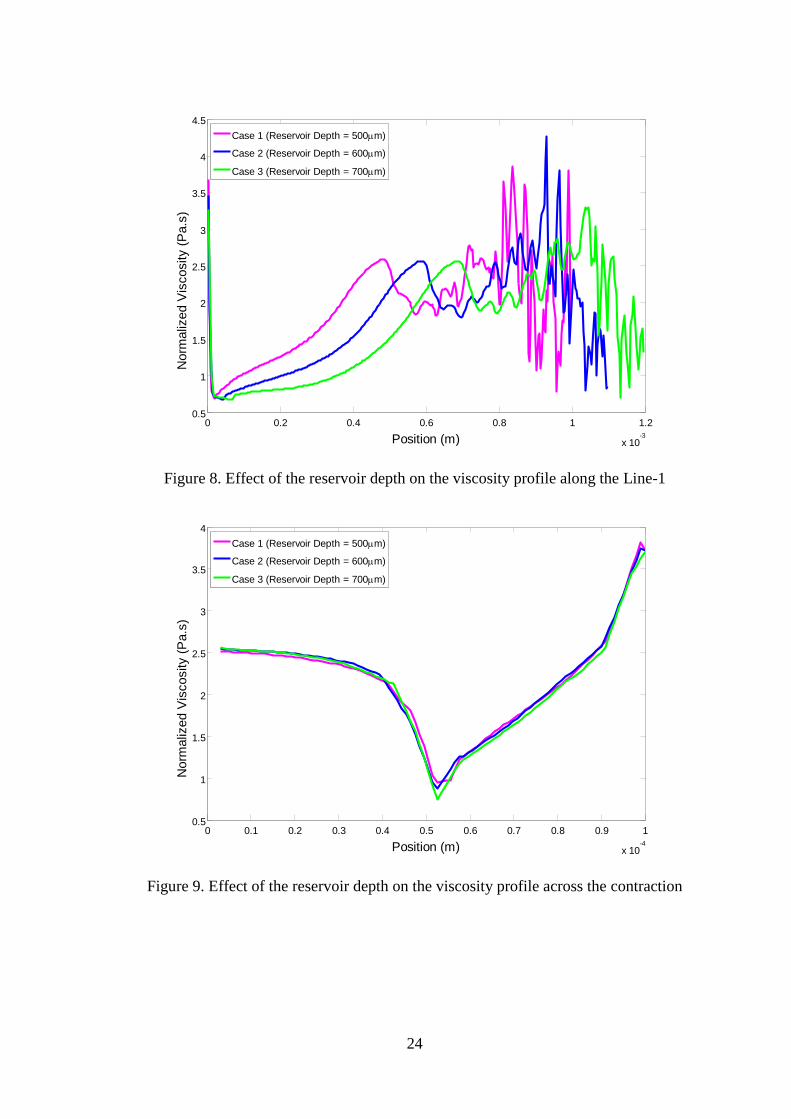
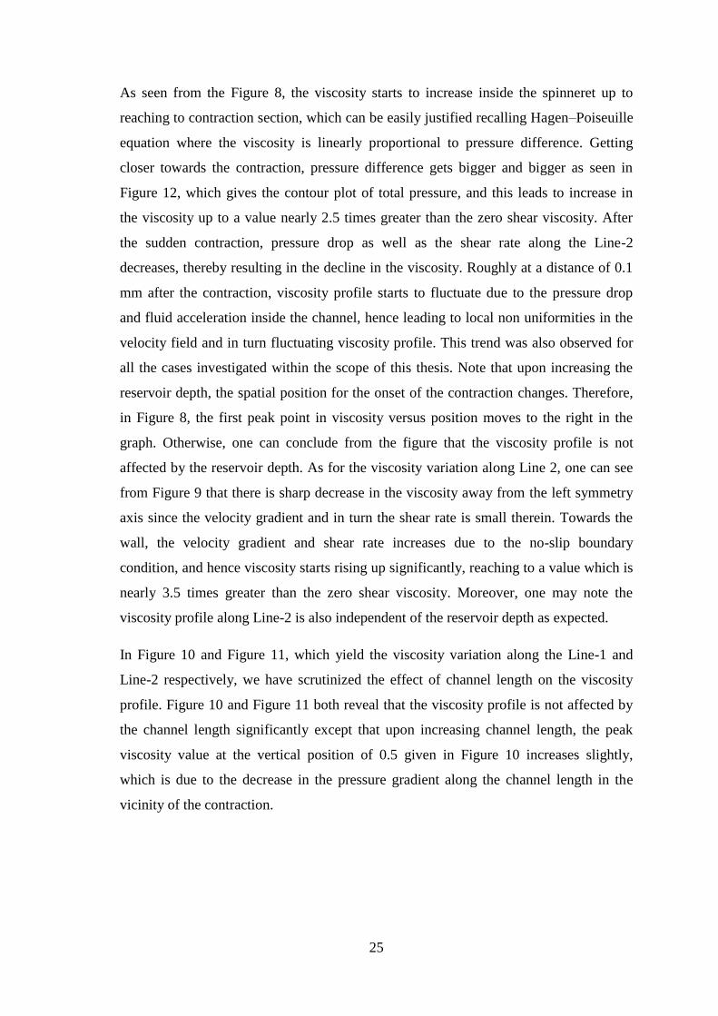
Here, initially, the results obtained upon changing reservoir depth will be presented for
both along Line-1 and Line-2. The Figure 8 and Figure 9 give the variation of the fluid
viscosity along the Line-1 and Line -2 of the computational geometry for different
reservoir depth.
24
Figure 8. Effect of the reservoir depth on the viscosity profile along the Line-1
Figure 9. Effect of the reservoir depth on the viscosity profile across the contraction
0 0.2 0.4 0.6 0.8 1 1.2
x 10-3
0.5
1
1.5
2
2.5
3
3.5
4
4.5
Position (m)
Norm
aliz
ed V
iscosity (
Pa.s
)
Case 1 (Reservoir Depth = 500m)
Case 2 (Reservoir Depth = 600m)
Case 3 (Reservoir Depth = 700m)
0 0.1 0.2 0.3 0.4 0.5 0.6 0.7 0.8 0.9 1
x 10-4
0.5
1
1.5
2
2.5
3
3.5
4
Position (m)
Norm
aliz
ed V
iscosity (
Pa.s
)
Case 1 (Reservoir Depth = 500m)
Case 2 (Reservoir Depth = 600m)
Case 3 (Reservoir Depth = 700m)
25
As seen from the Figure 8, the viscosity starts to increase inside the spinneret up to
reaching to contraction section, which can be easily justified recalling Hagen–Poiseuille
equation where the viscosity is linearly proportional to pressure difference. Getting
closer towards the contraction, pressure difference gets bigger and bigger as seen in
Figure 12, which gives the contour plot of total pressure, and this leads to increase in
the viscosity up to a value nearly 2.5 times greater than the zero shear viscosity. After
the sudden contraction, pressure drop as well as the shear rate along the Line-2
decreases, thereby resulting in the decline in the viscosity. Roughly at a distance of 0.1
mm after the contraction, viscosity profile starts to fluctuate due to the pressure drop
and fluid acceleration inside the channel, hence leading to local non uniformities in the
velocity field and in turn fluctuating viscosity profile. This trend was also observed for
all the cases investigated within the scope of this thesis. Note that upon increasing the
reservoir depth, the spatial position for the onset of the contraction changes. Therefore,
in Figure 8, the first peak point in viscosity versus position moves to the right in the
graph. Otherwise, one can conclude from the figure that the viscosity profile is not
affected by the reservoir depth. As for the viscosity variation along Line 2, one can see
from Figure 9 that there is sharp decrease in the viscosity away from the left symmetry
axis since the velocity gradient and in turn the shear rate is small therein. Towards the
wall, the velocity gradient and shear rate increases due to the no-slip boundary
condition, and hence viscosity starts rising up significantly, reaching to a value which is
nearly 3.5 times greater than the zero shear viscosity. Moreover, one may note the
viscosity profile along Line-2 is also independent of the reservoir depth as expected.
In Figure 10 and Figure 11, which yield the viscosity variation along the Line-1 and
Line-2 respectively, we have scrutinized the effect of channel length on the viscosity
profile. Figure 10 and Figure 11 both reveal that the viscosity profile is not affected by
the channel length significantly except that upon increasing channel length, the peak
viscosity value at the vertical position of 0.5 given in Figure 10 increases slightly,
which is due to the decrease in the pressure gradient along the channel length in the
vicinity of the contraction.
26
Figure 10. Effect of the channel length on the viscosity profile along the Line-1
Figure 11. Effect of the channel length on the viscosity profile across the contraction
0 0.2 0.4 0.6 0.8 1 1.2
x 10-3
0.5
1
1.5
2
2.5
3
3.5
4
Position (m)
Norm
aliz
ed V
iscosity (
Pa.s
)
Case 1 (Channel Length = 500m)
Case 4 (Channel Length = 600m)
Case 5 (Channel Length = 700m)
0 0.1 0.2 0.3 0.4 0.5 0.6 0.7 0.8 0.9 1
x 10-4
0.5
1
1.5
2
2.5
3
3.5
4
Position (m)
Norm
aliz
ed V
iscosity (
Pa.s
)
Case 1 (Channel Length = 500m)
Case 4 (Channel Length = 600m)
Case 5 (Channel Length = 700m)
27
Figure 12. Total pressure contours of the mixture
In Figure 13 and Figure 14 the viscosity profiles along Line-1 and Line-2 are provided
for three different channel widths namely, 100μm to 150μm and 200μm. It can clearly
be seen from Figure 13 and Figure 14 that widening the contraction section results in a
decrease in viscosity, which is due to the fact that when the contraction is larger,
pressure and velocity gradients become less severe, hence causing lower viscosities.
Having observed that narrower contraction results in drastic increase in viscosity values,
for the sake of completeness, it becomes prudent to shed some light on the effect of
corner geometry on the viscosity profile. To this end, we have also modeled the current
initial geometry with two different round corners having radius of 50μm and 100μm.
For these simulations, viscosity profiles are shown in Figure 15 and Figure 16 shows
that around contraction area, viscosity increases with increasing corner roundness.
Figure 16 verifies this situation but also it shows that viscosity across contraction
decreases significantly. The increase in the viscosity near to the symmetry boundary is
due to the increased pressure gradient therein. Nevertheless Figure 16 shows that the
viscosity decreases significantly across the contraction, especially at closer parts to the
corner, as a result of drastic decrease in the velocity gradient and shear rate, as well. For
case 9, where the contraction is the smoothest, viscosity at the edge decreases to half
compared to the standard case 1. These results show that, the roundness of a corner of a
contraction is of great importance for optimizing spinneret geometry.
28
Figure 13. Effect of the contraction width on the viscosity profile along the Line-1
Figure 14. Effect of the contraction width on the viscosity profile across the contraction
0 0.1 0.2 0.3 0.4 0.5 0.6 0.7 0.8 0.9 1
x 10-3
0
1
2
3
4
5
6
Position (m)
Norm
aliz
ed V
iscosity (
Pa.s
)
Case 1 (Contraction Width = 100m)
Case 6 (Contraction Width = 150m)
Case 7 (Contraction Width = 200m)
0 0.25 0.5 0.75 1 1.25 1.5 1.75 2
x 10-4
0.5
1
1.5
2
2.5
3
3.5
4
Position (m)
Norm
aliz
ed V
iscosity (
Pa.s
)
Case 1 (Contraction Width = 100m)
Case 6 (Contraction Width = 150m)
Case 7 (Contraction Width = 200m)
29
Figure 15. Effect of the corner roundness on the viscosity profile along the Line-1
Figure 16. Effect of the corner roundness on the viscosity profile across the contraction
0 0.1 0.2 0.3 0.4 0.5 0.6 0.7 0.8 0.9 1
x 10-3
0.5
1
1.5
2
2.5
3
3.5
4
4.5
5
5.5
Position (m)
Norm
aliz
ed V
iscosity (
Pa.s
)
Case 1 (Sharp Corner)
Case 8 (Corner Roundness = 50m)
Case 9 (Corner Roundness = 100m)
0 0.1 0.2 0.3 0.4 0.5 0.6 0.7 0.8 0.9 1
x 10-4
0.5
1
1.5
2
2.5
3
3.5
4
Position (m)
Norm
aliz
ed V
iscosity (
Pa.s
)
Case 1 (Sharp Corner)
Case 8 (Corner Roundness = 50m)
Case 9 (Corner Roundness = 100m)
30
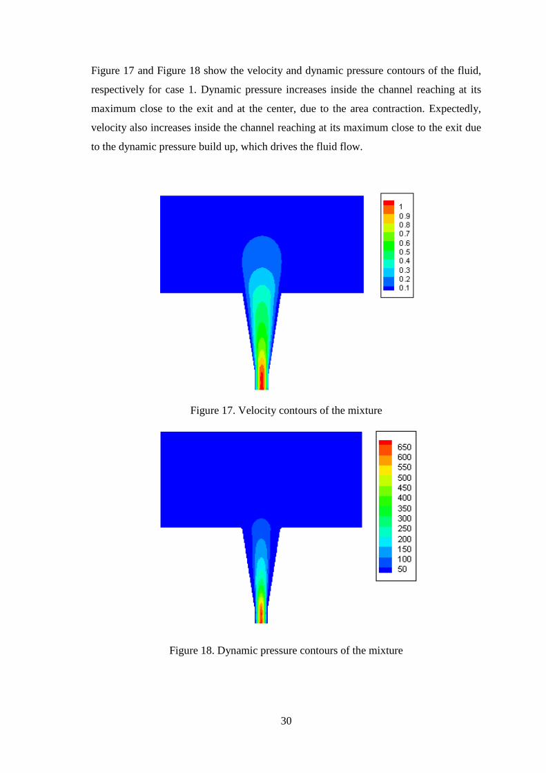
Figure 17 and Figure 18 show the velocity and dynamic pressure contours of the fluid,
respectively for case 1. Dynamic pressure increases inside the channel reaching at its
maximum close to the exit and at the center, due to the area contraction. Expectedly,
velocity also increases inside the channel reaching at its maximum close to the exit due
to the dynamic pressure build up, which drives the fluid flow.
Figure 17. Velocity contours of the mixture
Figure 18. Dynamic pressure contours of the mixture
31
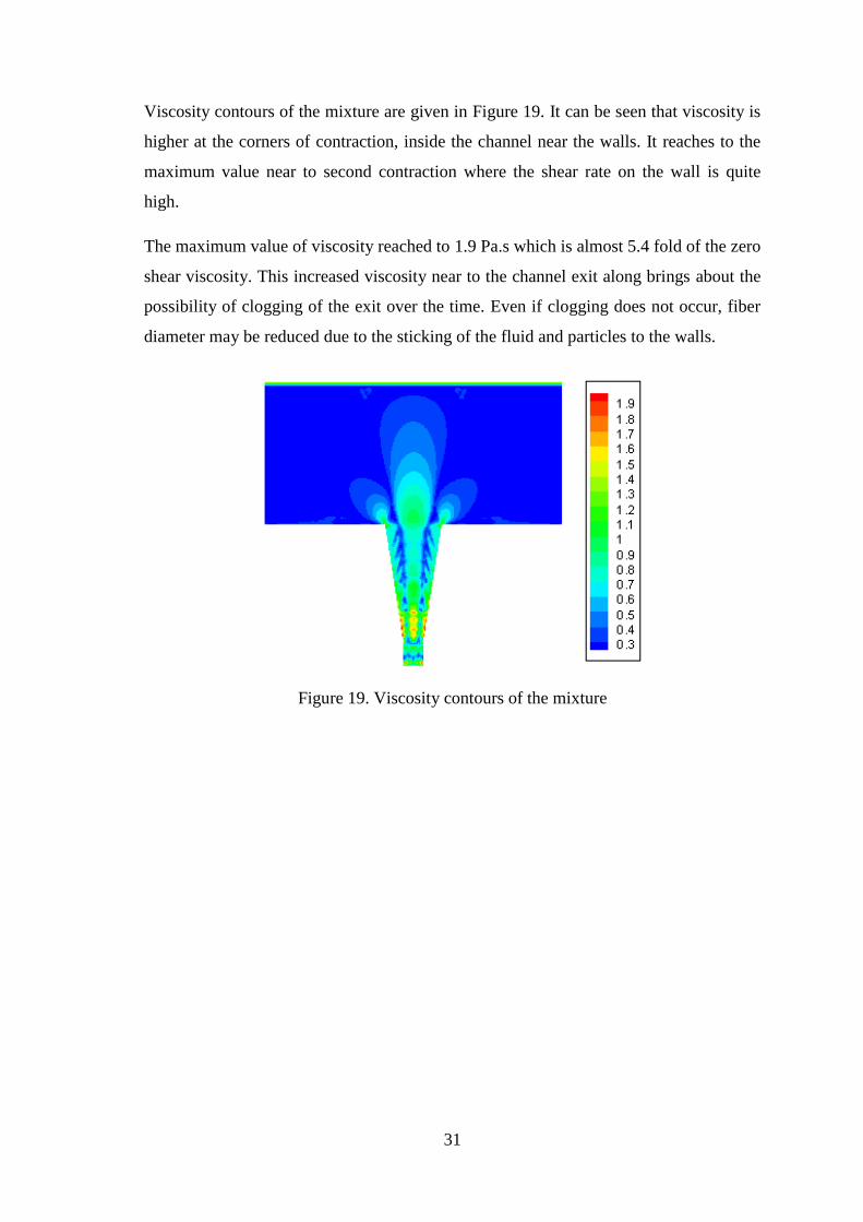
Viscosity contours of the mixture are given in Figure 19. It can be seen that viscosity is
higher at the corners of contraction, inside the channel near the walls. It reaches to the
maximum value near to second contraction where the shear rate on the wall is quite
high.
The maximum value of viscosity reached to 1.9 Pa.s which is almost 5.4 fold of the zero
shear viscosity. This increased viscosity near to the channel exit along brings about the
possibility of clogging of the exit over the time. Even if clogging does not occur, fiber
diameter may be reduced due to the sticking of the fluid and particles to the walls.
Figure 19. Viscosity contours of the mixture
32
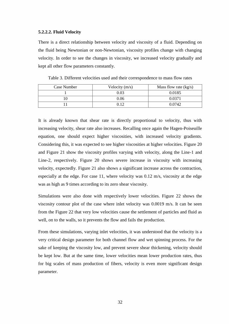
5.2.2.2. Fluid Velocity
There is a direct relationship between velocity and viscosity of a fluid. Depending on
the fluid being Newtonian or non-Newtonian, viscosity profiles change with changing
velocity. In order to see the changes in viscosity, we increased velocity gradually and
kept all other flow parameters constantly.
Table 3. Different velocities used and their correspondence to mass flow rates
Case Number Velocity (m/s) Mass flow rate (kg/s)
1 0.03 0.0185
10 0.06 0.0371
11 0.12 0.0742
It is already known that shear rate is directly proportional to velocity, thus with
increasing velocity, shear rate also increases. Recalling once again the Hagen-Poiseuille
equation, one should expect higher viscosities, with increased velocity gradients.
Considering this, it was expected to see higher viscosities at higher velocities. Figure 20
and Figure 21 show the viscosity profiles varying with velocity, along the Line-1 and
Line-2, respectively. Figure 20 shows severe increase in viscosity with increasing
velocity, expectedly. Figure 21 also shows a significant increase across the contraction,
especially at the edge. For case 11, where velocity was 0.12 m/s, viscosity at the edge
was as high as 9 times according to its zero shear viscosity.
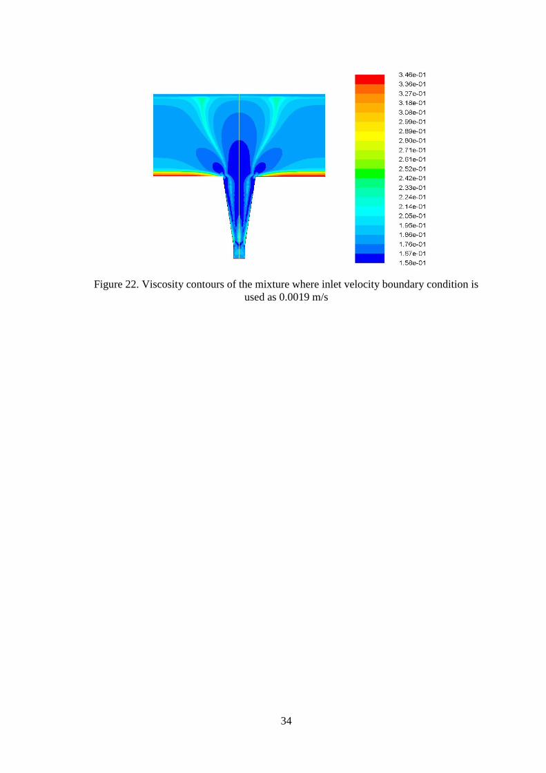
Simulations were also done with respectively lower velocities. Figure 22 shows the
viscosity contour plot of the case where inlet velocity was 0.0019 m/s. It can be seen
from the Figure 22 that very low velocities cause the settlement of particles and fluid as
well, on to the walls, so it prevents the flow and fails the production.
From these simulations, varying inlet velocities, it was understood that the velocity is a
very critical design parameter for both channel flow and wet spinning process. For the
sake of keeping the viscosity low, and prevent severe shear thickening, velocity should
be kept low. But at the same time, lower velocities mean lower production rates, thus
for big scales of mass production of fibers, velocity is even more significant design
parameter.
33
Figure 20. Effect of the velocity on the viscosity profile along the Line-1
Figure 21. Effect of the velocity on the viscosity profile across the contraction
0 0.1 0.2 0.3 0.4 0.5 0.6 0.7 0.8 0.9 1
x 10-3
0
2
4
6
8
10
12
14
Position (m)
Norm
aliz
ed V
iscosity (
Pa.s
)
Case 1 (Vinlet
= 0.03 m/s)
Case 10 (Vinlet
= 0.06 m/s)
Case 11 (Vinlet
= 0.12 m/s)
0 0.1 0.2 0.3 0.4 0.5 0.6 0.7 0.8 0.9 1
x 10-4
0
1
2
3
4
5
6
7
8
9
10
Position (m)
Norm
aliz
ed V
iscosity (
Pa.s
)
Case 1 (Vinlet
= 0.03 m/s)
Case 10 (Vinlet
= 0.06 m/s)
Case 11 (Vinlet
= 0.12 m/s)
34
Figure 22. Viscosity contours of the mixture where inlet velocity boundary condition is
used as 0.0019 m/s
35
CHAPTER 6
CONCLUDING REMARKS
This work has investigated several important parameters that affect the flow behavior of
non-Newtonian shear thickening multiphase fluids. Those parameters were geometry of
the spinneret and the flow rate. Within the scope of geometry study, reservoir depth,
channel length, contraction width and corner roundness were varied. The results showed
that depth of the reservoir does not affect the viscosity profile of the fluid whereas the
length of the channel has a small influence; nevertheless, none of these two parameters
can be considered to possess significant importance. Further results showed that sudden
contractions give rise to higher viscosities inside the spinneret due to higher shear rates,
and widening the contraction area reduces the increase in the viscosity. It was also
found that corners inside the geometry are shear rate concentrating areas, and by
rounding the corners, the effect of corner roundness on the viscosity can be alleviated.
Another significant outcome of this study is that the higher the flow rate, the viscosity
increases more dramatically due to the increasing shear rate while at the lower flow
rates, the decrease in viscosity is observed. However, at fairly lower flow rates, very
high viscosities were also observed due to the settling.
6.1. Future Work
To further improve the context of this study, the investigation of the particle size and
particle loading on the flow behavior inside the spinneret should be investigated.
Eulerian-Lagrangian Model and Dense Discrete Phase Model should also be used to be
able to test if they can provide additional physics for the problem considered in this
study. The geometry without symmetric boundaries should be used in simulations in
order to check if buoyancy arising from nanoparticles affects the viscosity and the
overall solution since there are some studies in the literature that showed the importance
of buoyancy in particulate non-Newtonian flows.
36
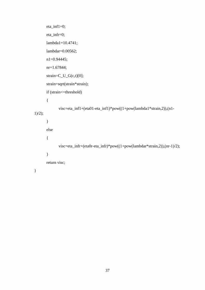
APPENDIX A
As described in section 4.2.3, the fluid used in the simulations was a so-called complex
fluid which showed shear thinning below a certain shear rate, and above that shear rate
it showed shear thickening. This complex viscosity behavior was fitted to the Carreau
fluid model by splitting the data into two parts as shear thinning and shear thickening,
and identified to the FLUENT by using a UDF, which was coded in-house by using C
programming language. There is the UDF code given below.
# include <udf.h>
# include <math.h>
# include <mem.h>
# include <sg_mphase.h>
# include <cmath.h>
# include <stdio.h>
DEFINE_PROPERTY(D11_PEG200_carreau_visc, c, t)
{
real strain;
real visc;
real eta01, eta0r;
real eta_inf1, eta_infr;
real lambda1, lambdar;
real n1, nr;
real threshold;
real cntrl;
threshold=95.78;
eta01=0.35517;
eta0r=0.23937;
37
eta_inf1=0;
eta_infr=0;
lambda1=10.4741;
lambdar=0.00562;
n1=0.94445;
nr=1.67844;
strain=C_U_G(c,t)[0];
strain=sqrt(strain*strain);
if (strain<=threshold)
{
visc=eta_inf1+(eta01-eta_inf1)*pow((1+pow(lambda1*strain,2)),(n1-
1)/2);
}
else
{
visc=eta_infr+(eta0r-eta_infr)*pow((1+pow(lambdar*strain,2)),(nr-1)/2);
}
return visc;
}
38
REFERENCES
1. Nakamura, A. and N. Akira, Fiber science and technology. 2000, Enfield, N.H.:
Enfield, N.H. : Science Publishers.
2. Hongū, T. and H. Tatsuya, New millennium fibers, ed. G.O. Phillips and M.
Takigami. 2005, Cambridge: Cambridge : Woodhead.
3. Elgafy, A. and K. Lafdi, Carbon nanoparticle-filled polymer flow in the
fabrication of novel fiber composites. Carbon, 2006. 44(9): p. 1682-1689.
4. Fourné, F. and F. Franz, Synthetic fibers : machines and equipment,
manufacture, properties : handbook for plant engineering, machine design, and
operation. 1999.
5. Masson, J.C., Acrylic fiber technology and applications, ed. J.C. Masson. 1995,
New York: New York : M. Dekker.
6. Catherall, A.A., J.R. Melrose, and R.C. Ball, Shear thickening and order–
disorder effects in concentrated colloids at high shear rates. Journal of
Rheology (1978-present), 2000. 44(1): p. 1-25.
7. Marinack, M.C., J.N. Mpagazehe, and C.F. Higgs, An Eulerian, lattice-based
cellular automata approach for modeling multiphase flows. Powder
Technology, 2012. 221: p. 47-56.
8. Deshpande, A.Y., et al., Rheology of complex fluids. 2010, Springer,: New York
; London. p. p.
9. Sochi, T., Flow of non-newtonian fluids in porous media. Journal of Polymer
Science Part B: Polymer Physics, 2010. 48(23): p. 2437-2767.
10. Chen, D.T.N., et al., Rheology of Soft Materials. Annual Review of Condensed
Matter Physics, 2010. 1(1): p. 301-322.
11. Bender, J. and N.J. Wagner, Reversible shear thickening in monodisperse and
bidisperse colloidal dispersions. Journal of Rheology (1978-present), 1996.
40(5): p. 899-916.
12. Wagner, N.J. and J.F. Brady, Shear thickening in colloidal dispersions. Physics
Today, 2009. 62(10): p. 27-32.
13. Hoffman, R.L., Discontinuous and dilatant viscosity behavior in concentrated
suspensions. II. Theory and experimental tests. Journal of Colloid and Interface
Science, 1974. 46(3): p. 491-506.
14. Barnes, H.A., Shear-Thickening (Dilatancy) in Suspensions of Nonaggregating
Solid Particles Dispersed in Newtonian Liquids. Journal of Rheology, 1989.
33(2): p. 329-366.
15. Boersma, W.H., J. Laven, and H.N. Stein, Shear thickening (dilatancy) in
concentrated dispersions. AIChE Journal, 1990. 36(3): p. 321-332.
16. Xu, D., C.-Y. Liu, and S.L. Craig, Divergent Shear Thinning and Shear
Thickening Behavior of Supramolecular Polymer Networks in Semidilute
Entangled Polymer Solutions. Macromolecules, 2011. 44(7): p. 2343-2353.
17. Barnes, H.A., A Handbook of Elementary Rheology. 2000: University of Wales,
Institute of Non-Newtonian Fluid Mechanics.
18. Kroger, M., R. Editor Applied, and [email protected], Rheology for
Polymer Melt Processing (J. M.-Piau and J.-F. Agassant, Eds.). 2000, ETH
Zurich; Applied Rheology.
19. Shaw, C.T., Using computational fluid dynamics. 1992, New York: Prentice
Hall. xviii, 251 p.
39
20. Kozic, M., et al., Numerical simulation of multiphase flow in ventilation mill and
channel with louvers and centrifugal separator. Thermal Science, 2011. 15(3):
p. 677-689.
21. Pirker, S., et al., Simulating coarse particle conveying by a set of Eulerian,
Lagrangian and hybrid particle models. Powder Technology, 2010. 204(2-3): p.
203-213.
22. Kaushal, D.R., et al., Flow of mono-dispersed particles through horizontal bend.
International Journal of Multiphase Flow, 2013. 52: p. 71-91.
23. Kalteh, M., et al., Eulerian–Eulerian two-phase numerical simulation of
nanofluid laminar forced convection in a microchannel. International Journal of
Heat and Fluid Flow, 2011. 32(1): p. 107-116.
24. Kamali, R. and A.R. Binesh, Numerical investigation of heat transfer
enhancement using carbon nanotube-based non-Newtonian nanofluids.
International Communications in Heat and Mass Transfer, 2010. 37(8): p. 1153-
1157.
25. Ding, Y., et al., Heat transfer of aqueous suspensions of carbon nanotubes (CNT
nanofluids). International Journal of Heat and Mass Transfer, 2006. 49(1–2): p.
240-250.
26. Yajie, R., X. Huaqing, and C. An, Effective thermal conductivity of nanofluids
containing spherical nanoparticles. Journal of Physics D: Applied Physics,
2005. 38(21): p. 3958.
27. Heris, S.Z., M.N. Esfahany, and G. Etemad, Numerical Investigation of
Nanofluid Laminar Convective Heat Transfer through a Circular Tube.
Numerical Heat Transfer, Part A: Applications, 2007. 52(11): p. 1043-1058.
28. Eesa, M. and M. Barigou, CFD analysis of viscous non-Newtonian flow under
the influence of a superimposed rotational vibration. Computers & Fluids, 2008.
37(1): p. 24-34.
29. Sahu, A.K., R.P. Chhabra, and V. Eswaran, Two-dimensional laminar flow of a
power-law fluid across a confined square cylinder. Journal of Non-Newtonian
Fluid Mechanics, 2010. 165(13-14): p. 752-763.
30. Manzar, M.A. and S.N. Shah, Particle distribution and erosion during the flow
of newtonian and non-newtonian slurries in straight and coiled pipes.
Engineering Applicationd of Computational Fluid Mechanics, 2009. 3(3): p. 25.
31. Hicks, C.I., et al., The shear rheology of bread dough: Analysis of local flow
behaviour using CFD. Food and Bioproducts Processing, 2012. 90(3): p. 361-
369.
32. Norton, T. and D.-W. Sun, Computational fluid dynamics (CFD) – an effective
and efficient design and analysis tool for the food industry: A review. Trends in
Food Science & Technology, 2006. 17(11): p. 600-620.
33. Fluent User's Guide 14.0, I. ANSYS, Editor. 2011.
34. Gidaspow, D., R. Bezburuah, and J. Ding, Hydrodynamics of circulating
fluidized beds: Kinetic theory approach. 1991. Medium: ED; Size: Pages: (8 p).
35. Syamlal, M., W. Rogers, and T.J. O`Brien, MFIX documentation theory guide,
in Other Information: PBD: Dec 1993. 1993. p. Medium: ED; Size: 49 p.
36. Huilin, L., et al., Hydrodynamic simulation of gas–solid flow in a riser using
kinetic theory of granular flow. Chemical Engineering Journal, 2003. 95(1–3): p.
1-13.
37. Gibilaro, L.G., et al., Generalized friction factor and drag coefficient
correlations for fluid-particle interactions. Chemical Engineering Science,
1985. 40(10): p. 1817-1823.
40
38. Lun, C.K.K., et al., Kinetic theories for granular flow: inelastic particles in
Couette flow and slightly inelastic particles in a general flowfield. Journal of
Fluid Mechanics, 1984. 140: p. 223-256.
39. Ozel, B.G., et al., Experimental study on the rheology of anisotropic, flocculated
and low volume fraction colloids. Korea-Australia Rheology Journal, 2014.
26(1): p. 105-116.
40. Eesa, M. and M. Barigou, CFD investigation of the pipe transport of coarse
solids in laminar power law fluids. Chemical Engineering Science, 2009. 64(2):
p. 322-333.
41. Bird, R.B., W.E. Stewart, and E.N. Lightfoot, Transport Phenomena. 2001:
Wiley.