Embed Size (px)
Citation preview

CFD-MatlabThermal Comfort Study
Design of a coupling system to exchange data betweenCFD programmes and a human thermal comfort model
Eva Bernat Fuentes (evabe235)
Linköping University | Department of Management and EngineeringMaster’s thesis, 30 credits | Master in Aeronautical Engineering
Spring 2020 | LIU-IEI-TEK-A–20/03892—SE

2

Linköping University | Department of Management and EngineeringMaster’s thesis, 30 credits | Master in Aeronautical Engineering
Spring 2020 | LIU-IEI-TEK-A–20/03892—SE
CFD-MatlabThermal Comfort Study
Design of a coupling system to exchange data betweenCFD programmes and a human thermal comfort model
Eva Bernat Fuentes (evabe235)
Academic supervisor: Jörg Schminder (LiU)Industrial supervisors: Roland Gårdhagen (LiU)Examiner: Matts Karlsson (LiU)
Linköping universitetSE-581 83 Linköping, Sverige
013-28 10 00, www.liu.se

2

Abstract
The general trend of increasing heat loads in modern passenger aircraft cabins e.g.caused by in-flight entertainment or novel energy sources, induces a rising demandfor efficient yet comfortable ventilation systems. Therefore, the typical design anddimensioning criteria of conventional Aircraft Cabin Ventilation system conceptsneed to be verified to avoid problems concerning the thermal sensation and comfortof the passengers. Fanger’s Predicted Mean Vote-method is traditionally used forestimating thermal sensation and comfort. The PMV method does not take into ac-count the human thermoregulatory system, therefore it progressively over-estimatesthe mean perceived warmth of warmer environments and the coolness of cooler en-vironments. Aircraft Cabin CFD models existing in the industry tend to make useof constant temperature boundary condition to define a human being. The com-promise on accuracy that this fact generates, brings the doubt about how makingmore realistic simulations. Human thermoregulatory models represent the humanbody from a thermokinetic point of view and they have been used for modelling thethermoregulation system. Their tissue heat transfer, thermal sensation and thermalcomfort calculation has been successfully validated under various steady-state andtransient indoor environment boundary conditions comparing the simulation resultsto measurements made with real human beings.
From an existing Matlab model of a human being (approximated with 9 layers and15 body parts) provided by Espuna [1], the main goal of this work is to connect it tothe three-dimensional cabin model in ANSYS Fluent developed by Raina et. al. [2].From it, local environmental conditions around a human body and the response ofthe human body to these conditions could be obtained, such as transient temperaturechanges at the skin. These last ones will be fed back to the CFD model to enable theeffect that the body has on the local environment. This two-way data transfer hasbeen thought to be important when modeling spaces with low air velocities accordingto Cropper [3], due to the impact that human body has on the local environment.The model regards an aircraft cabin. This simulation will have the goal of optimiz-ing the thermal comfort for the passengers. The ventilation conditions tested willbe Displacement Ventilation (DV) and a transient Thermal Comfort Model will beapplied at a local and global level for each human.


Acknowledgements
This master thesis was performed at Linköping University at the Department ofEngineering in the spring of 2020. With a deep sense of gratitude I would like to ac-knowledge all those who contributed significantly towards the successful completionof this project.
Especially, my supervisors Jörg Schminder and Roland Gårdhagen, who contributedin the day-to-day development issues of this project. Their dynamism, vision, sin-cerity and motivation have deeply inspired me. Emphasizing Jörg’s empathy andgreat sense of humour. I would also like to thank Hossein Nadali Najafabadi for hisvaluable input on developing the room model and vast knowledge on computationalheat transfer subject.
Besides my advisors, I would like to thank the examiner Matts Karlsson for the keeninterest to complete this thesis successfully, as well as his encouragement, insightfulcomments, and hard questions. Last but not the least I would like to thank myfamily and friends for their constant source of inspiration and support. Thanks toCarmen, for her constant support at personal fulfillment. Also to Leny, Matt, Caro,Paz, Alba, Mauri, Carla, Ricard and Alex who have been my family in Linköping.
Finally, I would like to dedicate this thesis to my grandfather Miguel, for being myinspiration and the first light of life - my engineer father and my raiser.


Nomenclature
Abbreviations and Acronyms
Abbreviation MeaningLiU Linköping UniversityCFD Computational fluid dynamicsCAD Computer aided designCPU Central processing unitHTRM Human Thermo-Regulatory ModelHVAC Heating, Ventilation and Air CoolingUDF User Defined FunctionPMV Predicted Mean VoteSTB Simplified Thermoregulatory Bio-Heat Equation
Latin Symbols
Symbol Description Unitsact activity level [met]
fcl clothing area factorhc convective heat transfer coefficient
[W ·m−2 ·K−1
]hr radiative heat transfer coefficient
[W ·m−2 ·K−1
]icl moisture permeability index from the
skin to the skin surfaceIcl clothing insulation [clo]
qconv convective heat transfer flux[W ·m−2
]qradlong
long-wave radiative heat transfer flux[W ·m−2
]qradsh short-wave radiative heat transfer flux
[W ·m−2
]qevap evaporative heat transfer flux
[W ·m−2
]to operational temperature [oC]
RH relative humidity
Greek Symbols
Symbol Description Unitsε Difference in the mean skin tempera-
ture between two data exchanges[oC]
β Thermal expansion coefficient [1/K]


Contents
1 Introduction 11.1 Literature study . . . . . . . . . . . . . . . . . . . . . . . . . . . . . 2
1.1.1 Objective . . . . . . . . . . . . . . . . . . . . . . . . . . . . . 4
2 Theory 72.1 Thermoregulatory Model . . . . . . . . . . . . . . . . . . . . . . . . . 7
2.1.1 Active system . . . . . . . . . . . . . . . . . . . . . . . . . . . 72.1.2 Passive system . . . . . . . . . . . . . . . . . . . . . . . . . . 72.1.3 Limitations . . . . . . . . . . . . . . . . . . . . . . . . . . . . 9
2.2 CFD . . . . . . . . . . . . . . . . . . . . . . . . . . . . . . . . . . . . 92.2.1 Meshing . . . . . . . . . . . . . . . . . . . . . . . . . . . . . . 92.2.2 Boussinesq Model . . . . . . . . . . . . . . . . . . . . . . . . . 10
2.3 Zhang’s thermal sensation and thermal comfort model . . . . . . . . 11
3 Method 153.1 Working in a simple connection between Fluent and Matlab . . . . . 15
3.1.1 MATLAB "AAS" Toolbox . . . . . . . . . . . . . . . . . . . . 163.1.2 Journal Files . . . . . . . . . . . . . . . . . . . . . . . . . . . 163.1.3 Back up Option: Profiles definition Within Ansys . . . . . . . 16
3.2 Modifications to the HTRM . . . . . . . . . . . . . . . . . . . . . . . 173.2.1 Clothing insulation . . . . . . . . . . . . . . . . . . . . . . . . 17
3.3 Interface connection between CFD Fluent and Fiala . . . . . . . . . 183.3.1 Fiala standalone work-mode. Uncoupled . . . . . . . . . . . . 193.3.2 Fiala-CFD work-mode. Coupled . . . . . . . . . . . . . . . . 203.3.3 Fiala model convergence . . . . . . . . . . . . . . . . . . . . . 203.3.4 The coupling algorithm . . . . . . . . . . . . . . . . . . . . . 20
3.4 CFD Design. Human in a 3D simplified Room . . . . . . . . . . . . . 223.4.1 Computer Aided Model (CAD) . . . . . . . . . . . . . . . . . 223.4.2 Model meshing . . . . . . . . . . . . . . . . . . . . . . . . . . 233.4.3 Physics to solve - Problem modelling . . . . . . . . . . . . . . 243.4.4 Solver setup . . . . . . . . . . . . . . . . . . . . . . . . . . . . 253.4.5 Boundary Conditions . . . . . . . . . . . . . . . . . . . . . . . 263.4.6 Validation I: procedure and verification. . . . . . . . . . . . . 263.4.7 Validation II: Heat transfer coefficients . . . . . . . . . . . . . 28
3.5 CFD Design Application. Human in the Cabin . . . . . . . . . . . . 343.5.1 CAD Model - Cabin . . . . . . . . . . . . . . . . . . . . . . . 343.5.2 Human model . . . . . . . . . . . . . . . . . . . . . . . . . . . 343.5.3 Model meshing . . . . . . . . . . . . . . . . . . . . . . . . . . 343.5.4 Solver setup . . . . . . . . . . . . . . . . . . . . . . . . . . . . 353.5.5 Boundary Conditions . . . . . . . . . . . . . . . . . . . . . . . 363.5.6 Thermal Comfort Study . . . . . . . . . . . . . . . . . . . . . 373.5.7 Calculation of Neutral skin temperature set points, Tskset . . 38

4 Results 394.1 Velocity Distribution in the Cabin with Humans . . . . . . . . . . . 394.2 Temperature Distribution in the Cabin with Humans . . . . . . . . . 404.3 Heat Transfer Coefficient on Humans for different couplings . . . . . 414.4 Thermal Comfort Study . . . . . . . . . . . . . . . . . . . . . . . . . 43
5 Discussion 455.1 Validation . . . . . . . . . . . . . . . . . . . . . . . . . . . . . . . . . 45
5.1.1 Case 0. A) Uncoupled Case. . . . . . . . . . . . . . . . . . . . 455.1.2 Case 0. A) Coupled Case. . . . . . . . . . . . . . . . . . . . . 46
5.2 Methodology . . . . . . . . . . . . . . . . . . . . . . . . . . . . . . . 465.3 Thermal Comfort Study . . . . . . . . . . . . . . . . . . . . . . . . . 475.4 Results . . . . . . . . . . . . . . . . . . . . . . . . . . . . . . . . . . . 475.5 Future work . . . . . . . . . . . . . . . . . . . . . . . . . . . . . . . . 48
6 Conclusions 49
Appendices 53
A First appendix 53A.1 Tables for convective heat transfer coefficient . . . . . . . . . . . . . 53A.2 Manikin body part segmentation . . . . . . . . . . . . . . . . . . . . 54A.3 Code . . . . . . . . . . . . . . . . . . . . . . . . . . . . . . . . . . . . 54

1 IntroductionNowadays, industry is highly interested in developing simulation systems that allowus to observe the human response in a given product during the design process,that’s why digital twins are created. Both the automotive and aeronautical industryare examples that invest in the development of human thermoregulation models topredict the resulting degree of comfort or discomfort a person experiences. Majoraircraft manufacturers, such as Boeing and Airbus, have been improving the comfortlevel of their cabins in order to meet this demand. As a consequence of it, a majorscope is then focused in providing effective design tools to improve building thermalperformance, improve occupant comfort and reduce energy consumption. One ofthese tools could be an integrative simulation which includes an aircraft cabin anda digital twin of a human.
The general trend of increasing heat loads in modern passenger aircraft cabins e.g.caused by in-flight entertainment or novel energy sources, induces a rising demandfor efficient yet comfortable ventilation systems. Although the industry is workingon a reversal of this general trend by identification and application of more sustain-able solutions for cabin related heat loads, novel ventilation concepts can supportthe effort to reduce the energy consumption of the environmental control system andmay be accompanied by other benefits like improved thermal passenger comfort orreduced cabin weight.
To approach this, computational fluid dynamics (CFD) is a computer modellingtechnique that is able to predict in considerable detail the complex patterns of air-flow and air temperature distribution. It has been used successfully to predict thelikely ventilation performance of many advanced naturally ventilated buildings (e.g.Short and Cook 2005 [4]). A CFD model provides temperatures and velocities ofairflow around a human body, whereas that the thermoregulatory model (HTRM)predicts the response of human body to detailed local environmental conditions. Thethermoregulatory model attemps to be a digital twin of a human body, which is adigital replica of a living or non-living physical entity, in terms of heat transfer forthis case. Numerical models are advantageous as it is extremely difficult to predicthuman responses for non-uniform conditions with high resolution by experiments.
In design practice, simple shaped blocks are often used to represent human occu-pants in CFD models and derive empirically based thermal comfort parameters suchas predicted mean vote (PMV) and predicted percentage of dissatisfed (PPD). PMVresults show that the environment is comfortable or not. This PMV model has be-come the internationally accepted model for describing the predicted mean thermalcomfort of occupants in indoor environments.The answer to “why we would need in-tegrated CFD and human models” seems simple: on the human side, we want moreresolution and accuracy in the calculation of heat transfer at the boundary; on theenvironment side, we want the environmental quality (e.g. thermal comfort) to beevaluated by human response rather than thermometer reading.
1
The new integrated simulation system, which couples the standalone CFD aircraftcabin simulation with the thermoregulatory model, will support engineers in thedetailed stages of the aircraft development process and in the development and op-timization of ECS and HVAC systems.
From an existing Matlab model of a human being (approximated with 9 layers and15 body parts) provided by Espuna [1], the main goal of this work is to connect it tothe three-dimensional cabin model on ANSYS Fluent developed by Raina et. al. [2].From it, local environmental conditions around a human body and the response ofthe human body to these conditions could be obtained, such as transient temperaturechanges at the skin. These last ones will be fed back to the CFD model to enable theeffect that the body has on the local environment. This two-way data transfer hasbeen thought to be important when modeling spaces with low air velocities accordingto Cropper [3], due to the impact that human body has on the local environment.
1.1 Literature studyThe computational thermal manikin, based on the coupled simulation of convection,radiation, moisture transport, and human thermal physiological model, was first de-fined and proposed by Murakami et al. (1997) [5]. A simplified body shape wasused without modeling body parts such as legs and hands separately. Tanabe et. at.(2002) integrated a 65-node human thermoregulatory model with a 3D model of amale body in CFD which incorporated radiation heat transfer.
Al-Mogbel (2003) [6] used a simplified shape to represent a human body in CFD inAnsys Fluent and coupled this with a two-node thermal regulatory model (Gagge et.al. 1986). Finally, a CFD code was obtained to map regions of Thermal Comfort,using 2 different thermal comfort indices. The model represented a standing humanin a naturally ventilated room. Its aim was determining the total (sensible+latent)heat transfer of the human body, and to predict thermal comfort zone in the room.
More recently, Cropper et al. (2010) [3] have investigated and validated with numer-ical and experimental work, the same topic modelling a standing human subject ina naturally ventilated environment in the context of a non-domestic building. TheInstitute of Energy and Sustainable Development (IESD) developed a new versionof Fiala creating IESD-Fiala. Using IESD-Fiala for the thermoregulatory model,Ansys CFX as the CFD software and CFX Expression Language (CEL) functionsas the communication interface between both softwares. The reason for embeddingIESD-Fiala model in CFD is motivated since in transient studies the CFD softwaremust have the possibility to update boundary conditions for each time step duringsolver execution cycle. However, differences between the simulations and experimen-tal results were not published. Both naked [3] and clothed [7] manikins were testedand heat transfer coefficients for individual body parts were reported.
2
Fiala (2004) [8] used the method of exchanging data between two models for carsindustry; consisting of network sockets and data files. It was used in the INKAcar simulator which used a simple approach using locally stored files. INKA isstate-of-the-art simulation software that provides comprehensive predictions of theprevailing, time-varying thermal environment in automobiles. From it, we can obtainthe knowledge of how to connect the human model with the car. In order to get real-istic simulations for the liked car - occupant system, thermal interactions occurringbetween the passengers and the indoor environment were modelled. These includee.g. the warming of the occupied zone by the realease of bodily heat and changesin the water vapour content of the air due to respiration and moisture evaporationfrom the body surface, as well as the dynamic heat loss from body parts in contactwith car surfaces. To capture these effects it was imperative that the new simulationsystem enabled a bi-directional, dynamic data exchange between the models. Toachieve it, the simulation deploys as two parallel processes that are coupled via acommunication interface with controls the exchange of the simulated data for eachtime step of a simulation run. It will be important that there is a matching betweenevery geometry part, (i.e. every single part of the body in which it is splitted), ofthe CFD model mesh and the thermoregulatory model mesh.
Dixit et. al. (2015) [9], worked with a seated human model in a ventilated roomand used Ansys Fluent with the help of a User Defined Function (UDF, writtten inC script) to assign the temperatures of the skin interface from the thermoregulatorymodel. With UDFs the user can define a customized boundary profile (like the tem-perature of the skin, obtained from the HTRM) which varies as a function of timeand/or space (for instance, every part of the body can be defined with a differenttemperature). As it can be found in the ANSYS Fluent UDF manual [10], to definethe temperature at a boundary, the "Define Profile" macro is needed, with which thedesigner can customize the boundary profile as written previously. The thermoregu-latory model used is based on Fanger’s model (which accounts for passive response)but with adding the Simplified Thermoregulatory Bio-Heat Equation (STB) (whichaccounts for active response). That will fix the fact that Fanger’s model by itself isuncapable to account active thermoregulatory activities such as vasomotion, sweat-ing and shivering etc. which are inherent from transient simulations. Since theSTB equation can be solved within the CFD tool itself, it also avoids the need of aseparate standalone model for human body thermoregulation simulation. The innerhuman was solved inside Fluent, in which surfaces, the equation of the simplifiedthermoregulatory bio-heat equation is applied as a Boundary Condition in a UDFfile. It contains two boundary conditions: the skin boundary condition and the coreboundary condition.
Martinho et. al. (2012) [11] developed a study of a human manikin in a standard3D-room comparing it with experimental results. The aim was evaluating possibleCFD errors and determining the importance of considering an appropriate turbulencemodel (k- ω SST vs. k-ε) and the contribution of radiation effects. It was concludedthat approximately 40% of heat transfer in human body was due to radiation (vs.convection), and that SST was a better model to predict heat fluxes near wall.
3

Yang (2008) [12] described specifically in practical words, how to adapt Fiala codecalculations in order to interface IESD-Fiala model with ANSYS CFX. Some of heattransfer components from Fiala were simplified. They neglected conductive andshort wave radiation (irradiation) heat transfer effects because of being insignificant.They focused on heat transfer due to convection, long wave radiation and evapo-ration. Likewise Cropper [3] did, but added, however, short wave radiation. Localeffects may be of interest if, for example, incident short-wave radiation is locally ab-sorbed at parts of the body while the air condition supplies a stream of air to someof the other parts.
Yang (2017) [13] revealed the importance of using a multinode thermoregulatorymodel, such as Fiala is. First researchers, like Murakami (1999) [14], used a two-nodethermal model in the coupling system. When a two-node thermal model is applied,the thermal responses of individual body segments cannot be predicted. Actually,human beings are always exposed to non-uniform environments and human ther-moregulatory highly depends on local heat transfer characteristics. Therefore, it isinappropiate to evaluate thermal physiological responses at whole body level and amulti-node thermal model is required.
Gao (2005) [15] critically reviewed issues in CFD simulation using a numerical ther-mal manikin, such as turbulence model selection, grid generation and boundaryconditions. The low Reynolds number k-ε model performs better in the predictionof heat loss from human body while the standard k- model and RNG k-ε model aresufficient if the emphasis is on airflow field.
De Dear (1996) [16] provided an experimental study of convective and radiative heattransfer coefficients for individual human body segments for a human female nudebody, which is until today, the most accepted study. Nevertheless, this study splittedthe body in big areas, like only 8 body parts.
Sorensen et Voigt (2003) [17] developed a CFD model of flow and heat transferaround a seated naked human body, providing details such as a plot graph of veloci-ties above the human head, which eases verification of new CFD models, such as theone that is developed at the present work. Even though, Sorensen’s model was onlyCFD based, with a constant temperature in the skin of the human as a boundarycondition. It was not connected to a HTRM.
1.1.1 Objective
The aim of this master thesis consists of developing an integrated coupled simula-tion system for predicting both the dynamic, non-uniform environmental conditionsin an aircraft cabin (CFD) and the human physiological and perceptual reponsesunder these complex circumstances. This simulation will have the goal of improvingthe thermal comfort for the passengers. For that, different ventilation conditions willbe compared in order to see which one offers the best thermal comfort.
4

To split this big task, there are sub-objetives:
• To create the software connection with a simple domain in Ansys and Matlabas an example (AAS Toolbox).
• To implement a 3D-room CFD case to analyze software connection with asingle human manikin. Design a 3D-room CAD and couple it with the manikingeometry.
• To setup a CFD model running a RANS Turbulence model to simulate naturalventilation.
• To couple thermoregulatory model in Matlab with the CFD model in ANSYSby means of the first connection done (AAS Toolbox) to analyse heat transfertrends.
• To design the coupled case for the aircraft cabin. To split the mesh of thehuman manikin for having the 15 parts required by the HTRM.
• To run the RANS Turbulence model that is already provided by Raina et. al.[2] with the coupling of AAS Toolbox.
• To analyze the different ventilation systems and study their performance onthermal comfort by evaluating velocity and temperature profiles measured atlocations close to the occupants in the cabin.
Limitations
The present thesis doesn’t mean to focus on developing a new case of a CFD studybut studying heat transfer effects between humans and the environment. This meansthat the following features are not going to be studied:
• CFD of the aircraft cabin study provided by Raina et. al.[2] is going to betreated as a special case of application and the CFD model is not going to beimproved.
• HRTM model is quite elementary and is not either the focus of improvement.
Moreover, concerning the used model there are also some inherent limitations. Firstly,the detailed 3-D models of human in the CFD environment represented the nakedbody, which is unlike the case in every day environment. It is perceivable that theshape and posture of the model may have a significant impact on the local convectiveand radiant heat transfer coefficients. Models of clothed body should be studies toquantify such impact. Secondly, evaporation at the skin surface is a complex process,which is connected with moisture transportation due to convection. In the studieswhere evaporation was considered, empirical methods rather than CFD were used.
5


2 Theory
2.1 Thermoregulatory ModelThe thermoregulatory Model that has been used was developed by Espuna [1] in 2017for Matlab software. This HTRM model is based on Fiala’s model (1998) which hasbeen adapted to pressure changes in altitude for aeronautical applications and alsowith some modifications from Tanabe (2002) for clothing [1]. This Fiala model usesenvironmental parameters, such as the temperature at the skin surface, to predictthe response of the human thermoregulatory system to these external stimuli over aperiod of time.
Fiala thermal comfort model consists of two interacting systems: the controllingactive system and the controlled passive system.
2.1.1 Active systemThe active system is in charge of regulating body temperature to mantain a stablevalue of temperature in the body core. The thermoregulatory system activates fourkinds of response to regulate the body temperature: vasodilatation, perspiration,vasoconstriction and shivering. In hot conditions, vasodilatation and sweating areactivated, to excrete moisture at the skin which evaporates producing the cooling ofthe body. However, in cold conditions, vasoconstriction is activated with shivering,an increase of the metabolic internal heat generation by contraction of muscles.
The active system was developed by means of statistical regression using measureddata from several experiments ranging from steady state to transient cold stress,cold, warm and hot stress conditions, and different activity levels, from low to highexercise.
2.1.2 Passive systemThe passive system is a multi-segmental, multi-layered representation of discretizedhuman body and information about geometrical body properties.
The body is represented as 15 spherical and cylindrical elements built of annularconcentric tissue layers with the appropriate thermo-physical properties and phys-iological functions. In each of the 15 so called elements or body parts, there is amaximum of 9 tissue layers, which would correspond into a discretization of 135nodes in total amount. Each tissue can be made of one of the following elements:brain, lung, viscera, skin, bone, muscle. (See Figure 1).
The sizes and composition of the 15 body parts, are contained in the Matlab script”HTRMbasic.m” which enables easily different body characteristics to be modeled.
7

Figure 1: Fiala’s approach to the human discretization. 15 body parts and segmenta-tion. Extracted from [18]
Heat transfer equations in the model account for convection and radiation (longand short-wave) with the environment; internal heat production and blood heat ex-change; and clothing insulation from the environment.
Figure 2: Sector-wise discretization of the concentric layer model and treatment ofheat exchange with the ambient. Extracted from [18]
Clothing might be treated as additional layer that differs from the original Fialamodel as shown in Figure 2. Via blood circulation, metabolic heat is transportedto different elements and by radial conduction to the body surface where it is trans-ferred to the environment by convection, radiation, evaporation and, if applicable,respiration and conduction, on the basis of the bioheat equation proposed by Pennes(1948), Equation 1.
8

k(∂2T
∂r2+ω
r+∂T
∂r
)+ qm + ρblwblcbl(Tbla − T ) = ρc
∂T
∂t(1)
The differential equation models the heat transfer in human tissues with a cylindri-cal model, where k represents the tissue conductivity (W ·m−1 ·K−1), T the tissuetemperature (oK), r the radius (m) and ω is a dimensionless geometric factor ( ω= 1 for cylinders, ω = 2 for spheres). qm denotes the metabolic heat production(W/m3), which consists of a basal value plus the local autonomic thermoregulationwhile shivering. The last therm on the left-hand side of Equation 1 represents bloodperfusion, where ρbl stands for the density (kg/m3), wbl for perfusion rate (s−1), cblfor the heat capacity (J · kg−1 · K−1) and Tbl,a for the arterial blood temperature(C). For the blood circulation, a central blood pool is assumed by modelling anexchange within the arterial and venous vascular system and by neglecting the heatstorage within the vascular system. The metabolism qm and blood perfusion rate wblare thereby influence by the active control system. Only radial heat conduction isconsidered as the surface areas of the interfaces between two sectors are insignificantcompared with the surface areas of the sectors themselves. With respect to the skinmoisture evaporation, a partial differential equation is used to describe the moistureaccumulation and sweat production as predicted by the active system. For the respi-rative exchange, which again depends on the metabolism, it is distinguished betweendry and latent heat exchange, which is distributed along the pulmonary tract.[18]
According to Fiala’s work [19], the present model represents an average male weight-ing 73.5 kg, with 14 % of body fat, a skin surface area of 1.86 m2, a cardiac outputof 4.9 L/min, and a basal metabolic rate of 87.1 W.
2.1.3 LimitationsThe model is simplified in such a way that it presenst the following limitations [1]:
• Only radial heat transfer is considered through the cylinders.
• Heat variations in the longitudinal direction are neglected.
• Every part of the body is represented as a cylinder or a sphere.
2.2 CFDIn this section, several basic CFD concepts that will be used in the Method sectionare explained to ease the general understanding for the reader.
2.2.1 MeshingMeshing strategy is focused on three fundamental aspects: accuracy, efficiency andease of generation.
9
Accuracy involves to have an adequate quality mesh in order to pre achieve conver-gence and a viable result. Efficiency means that cell count and element type areadequate to the available time to solve and isn’t big enough to outgrow the actualRandom Access Memory (RAM). And finally, ease of generation which means thatsetting up is going to take a reasonable amount of time. The goal is to find bestcompromise between accuracy, efficiency and ease of generation.
Fluent Meshing is similar to Workbench Meshing but it’s more powerful though. Ithas more element types and more flexible customizations. Specially, it is consideredto be an optimal tool to develop high quality meshes for complex geometries in aneasier and faster way.
Inside Fluent Meshing there are several element types that can be created, each fortheir own benefit. Prisms are used to capture the boundary layer, the quality can bereduced around complex surfaces so it’s important to make sure that the geometryis repaired. A tech grid is used to resolve areas of high complexity with good reso-lution. However, it can take quite a time to solve. The next best thing for that isthe polyhedral grid that it combines a couple of tet elements to make a polyhedralelement. The benefit of that is that it can actually reduce cell count and CPU timeat the expense of requiring extra RAM. In case a hexahedral grid is possible to bedue, it has the advantages versus the poly that it’s got a smaller grid so it shouldtake quicker to actually run. When a hexahedral grid is not possible to be due anda polyhedral would require high computational capacities, an intermediate solutionsuch as a polyhex mesh could be optimal.
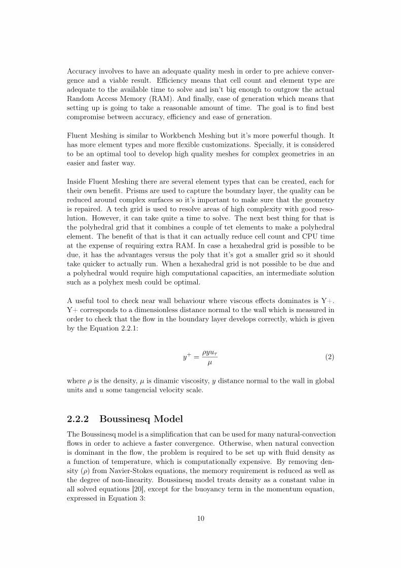
A useful tool to check near wall behaviour where viscous effects dominates is Y+.Y+ corresponds to a dimensionless distance normal to the wall which is measured inorder to check that the flow in the boundary layer develops correctly, which is givenby the Equation 2.2.1:
y+ =ρyuτµ
(2)
where ρ is the density, µ is dinamic viscosity, y distance normal to the wall in globalunits and u some tangencial velocity scale.
2.2.2 Boussinesq ModelThe Boussinesq model is a simplification that can be used for many natural-convectionflows in order to achieve a faster convergence. Otherwise, when natural convectionis dominant in the flow, the problem is required to be set up with fluid density asa function of temperature, which is computationally expensive. By removing den-sity (ρ) from Navier-Stokes equations, the memory requirement is reduced as well asthe degree of non-linearity. Boussinesq model treats density as a constant value inall solved equations [20], except for the buoyancy term in the momentum equation,expressed in Equation 3:
10

(ρ− ρ0) · g ≈ −ρ0β(T − T0) · g (3)
Where ρ0 is the (constant) density of the flow, T0 is the operating temperature, and βis the thermal expansion coefficient. Equation 3 is obtained by using the Boussinesqapproximation to eliminate ρ (the density at each point of the domain) from thebuoyancy term. Equation 3 is obtained by using the Boussinesq approximationdefined in Equation 4.
ρ = ρ0 · (β(T − T0)) (4)
This approximation is accurate as long as changes in actual density are small; specif-ically, according to the Manual [20], the Boussinesq approximation is valid whenEquation 5 is fulfilled.
β · (T − T0)� 1 (5)
In practical words, errors of 1% at room temperature are obtained if Equation 6 isfulfilled. In the case of room ventilation with a human in the room, the maximumdifference of temperatures would correspond to the values: T = 34oC (on the headof the human) and T0 = 21oC which is the room temperature, this would lead to adifference of 13oC, where Boussinesq model is valid.
∆T =
T − T0 < 2oC Water
T − T0 < 15oC Air
(6)
2.3 Zhang’s thermal sensation and thermal com-fort model
Zhang (2010) ([21], [22]) developed a thermal sensation model to predict local andoverall sensations, and local and overall comfort in non-uniform transient thermalenvironments. The model predicts human subjective responses to the environmentfrom thermophysiological measurements or predictions. From body HTRM parame-ters such as the local skin and core temperature, the local thermal sensation can beobtained. The overall thermal sensation and comfort are calculated as a function ofthe local skin temperatures and the core temperature, and their change over time.These parameters are calculated for each of the body parts. Zhang’s model seems tobe more applicable than the usually used PMV model, which rests on steady stateheat transfer theory and this state never precisely occurs in daily life. Moreover, deDear and Brague (1998) found that the PMV overestimates the subjective warmthsensations of people in warm naturally ventilated buildings. [16]
Zhang (2010) proposes that the local thermal sensation Slocal, (see Eq. 7), is alogistic function of local skin temperature, presented as the difference between thelocal skin temperature and its set point:
11

(7)Slocal = 4
(2
1 + e−C1·(tskin,loc−tskin,loc,set)−K1[(tskin,loc−tskin)−(tskin,loc,set−tset)]
),
+C2idtskin,loc
dt+ C3i
dtcoredt
where tskin,loc is the local skin temperature, tskin,loc,set is the local skin set pointtemperature, tskin is the mean whole-body skin temperature and tset is the meanwhole-body skin set point temperature. K1, C1, C2 and C3 are specific regressioncoeffficients for every body part. When the derivatives of skin and core temperatures(second and third term on the right-hand side of the equation) are zero, the modelpredicts thermal sensation in a steady state condition. In the method section, it isexplained how the set point temperatures were calculated. These set points are thetemperatures at which there is a neutral thermal reaction of the body.
The logistic function shows a linear relationship between the skin temperature andthermal sensation when the skin temperature is near its set point, but levels off whenthe skin temperature differs from the set point. When the local skin temperaturediffers from the local skin temperature set point, the sensation reaches the sensationscale limits between +4 and -4, ranging from very hot to very cold, (see Table 4).
Table 4: Thermal Sensation index (Zhang 2010).
Index Thermal sensation
4 very hot3 hot2 warm1 slightly warm0 neutral-1 slightly cool-2 cool-3 cold-4 very cold
The overall thermal sensation S0 is a weighted average of all the local sensations:
S0 =
∑(weightiSlocal,i)∑
(weighti)(8)
where Slocal represents the local sensation for segment i, and weighti is the weight-ing factor for that segment. The weighting factors are based on measurement resultsfrom 3 different types of conditions: uniform environments, step change transientbetween 2 different environments, and heating/cooling of local body parts undercool/warm ambient environments.
Local Comfort by Zhang is a piecewise linear function of local and overall thermalsensations calculated in Equation 9. It depends of regression coefficients for every
12
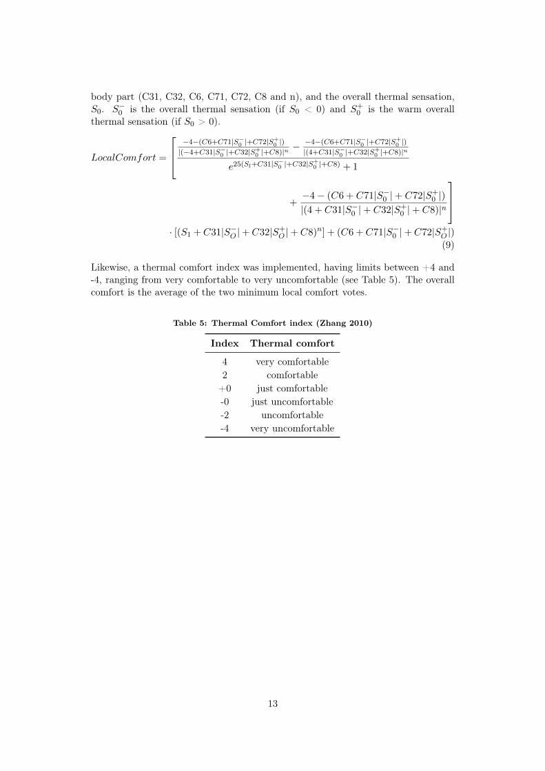
body part (C31, C32, C6, C71, C72, C8 and n), and the overall thermal sensation,S0. S−0 is the overall thermal sensation (if S0 < 0) and S+
0 is the warm overallthermal sensation (if S0 > 0).
LocalComfort =
−4−(C6+C71|S−0 |+C72|S+
0 |)|(−4+C31|S−
0 |+C32|S+0 |+C8)|n −
−4−(C6+C71|S−0 |+C72|S+
0 |)|(4+C31|S−
0 |+C32|S+0 |+C8)|n
e25(Sl+C31|S−0 |+C32|S+
0 |+C8) + 1
+−4− (C6 + C71|S−0 |+ C72|S+
0 |)|(4 + C31|S−0 |+ C32|S+
0 |+ C8)|n
· [(S1 +C31|S−O |+C32|S+
O |+C8)n] + (C6 +C71|S−0 |+C72|S+O |)(9)
Likewise, a thermal comfort index was implemented, having limits between +4 and-4, ranging from very comfortable to very uncomfortable (see Table 5). The overallcomfort is the average of the two minimum local comfort votes.
Table 5: Thermal Comfort index (Zhang 2010)
Index Thermal comfort
4 very comfortable2 comfortable+0 just comfortable-0 just uncomfortable-2 uncomfortable-4 very uncomfortable
13


3 Method
In this section, the full methodology is going to be thoroughly explained in a chrono-logical order. First, how the first connection between programmes had been done.Secondly, what were the modifications to the thermoregulatory model to be able tointerface it with a CFD programme. Inner modifications to the thermoregulatorycode were required to develop a system of inputs and outputs. Thirdly, how was thecoupling algorithm developed, in order to give response at the question to when andhow data exchange should take place. Finally, the construction of the CFD cases inAnsys Fluent and their validation.
3.1 Working in a simple connection between Flu-ent and Matlab
There are a couple of ways to connect Matlab results with Fluent: one is betweenshared files, which involves the use of Fluent journal and Gambit, and the other oneis scripting Fluent directly from Matlab with the "AAS" Server Mode.
Figure 3 shows the two available models that have to be connected so that each oneof them can be improved. The interface that is provided by Ansys to connect Fluentwith Matlab, permits to obtain the same output in Matlab as if you were writting thecommands in Ansys console. It also demonstrates how to execute Fluent commandsfrom a Matlab session. The following subsections show the options that have beenfound so far to be able to connect the two softwares.
Figure 3: The subjects of the study.
15
3.1.1 MATLAB "AAS" ToolboxMatlab "AAS" is a toolbox available for Matlab in which it is used As A Server(AAS) for Ansys programs. This seems to be the best option to connect ANSYSand MATLAB, if the user does not have high programming skills and overall knowl-edge of programming languages, among which, especially programs like FORTRAN,JAVA, C++. The toolbox can be downloaded from the ANSYS customer serviceportal and easily installed on MATLAB. It is also pretty straight forward to makea first connection with ANSYS. This is the tool that was finally used. It allows totransfer parameter variables easily between two softwares. The manual "ANSYS as aServer Example: MATLAB setup" [23] has been used to install Ansys Fluent serverin the personal computer. The manual "ANSYS Fluent as a Server User’s Guide"[24] can be consulted in order to understand Matlab commands which produce theactions in Fluent and control the whole simulation.
Since the functions of writing and reading parameters from Fluent that were ex-plained in the manual [24] (page 49), were not working, these had to be implementedfor the present work.
3.1.2 Journal FilesJournal files also seems to be a good option to be implemented to connect MATLABand ANSYS to realize a dynamic connection between them. In fact, they are usedto automate a series of commands instead of inputting them step by step in thecommand line [20]. They can also be used to create a record of the input to aprogram session for later reference. The only problem is that they do not seem to beas straight forward to use like the MATLAB "AAS" Toolbox and at the same timethey do not seem to be as powerful as UDFs. However, there could be a chance touse the "AAS" Toolbox together with journal files. Then the three tools found toconnect the two models might in the end be used together to create the best possibleconnection.
3.1.3 Back up Option: Profiles definition Within AnsysAs a backup option, the profiles definition option under the "boundary conditions"feature within ANSYS could be utilized. With this, the user can read and/or writeprofiles defined usually as .csv or .prof files. So, for instance, an array or a ma-trix obtained from the MATLAB model can be saved with these formats and, lateron, uploaded manually to ANSYS to be assigned as a boundary condition to thepassengers inside the Fluent model.
16

3.2 Modifications to the HTRMThe thermoregulatory model provided was fully working in a standalone mode.Nonetheless, it was required to be modified to create input parameters for a CFDprogram, and that means, to substitute the external physics ocurring out of theskin, such as environmental convection and radiation. The original thermoregula-tory model considered that air flow was approaching towards the human body witha constant velocity and at an average temperature. Moreover, extra modificationshad to be done such as the calculation of clothing temperature, which was missingin the implementation of the code.
3.2.1 Clothing insulation
The HTRM provided by Espuña [1] treats clothing insulation as Tanabe (2002) [25].The cloth isn’t modeled as an extra layer of the discretized body, but rather as a"thermal resistance". It means, there isn’t specifically a node for the cloth layer,but the heat transfer coefficient from the environment to the skin, is reduced by anempirical equation in order to account for insulation effects (see Equation 10).
ht =1
0.155 · Icl + 1(hc+hr)fcl
(10)
Where ht is the equivalent total heat transfer coefficient, hc is the convective heattransfer coefficient, hr is the radiative heat transfer coefficient, Icl is the moisturepermeability index from the skin to the skin surface, and fcl is the clothing areafactor.
For the present work, a naked person has been tested in order to be able to compareresults with Cropper [7] and available experimental results. Nevertheless, in case infuture works this coupling system investigation could further developed, it has beenmodified also for having clothing option. The Icl that was set as a uniform value,has been modified to the Icl values for the Kansas State Uniform (KSU) + summerclothing that has been widely used in the research and specifically in the works ofCropper (2009,2010) [3], Yang [13], Zhang et. Yang [12]. The aim is to ease thepossible comparison in case a clothed body might be simulated.
Moreover, the calculation of the temperature of the cloth, Tcl has been added, asshows Equation 11. It will make possible to state the temperature of the surface inthe CFD case when a clothed body is treated.
Tcl = (Tsk − Tair) ·1
hc+hr1ht
+ Tair (11)
Where Tcl is the cloth temperature, Tsk is the temperature of the skin and Tair isthe operative room temperature of the sorrounding air.
17

3.3 Interface connection between CFD Fluentand Fiala
To interface Fiala model with the commercial package, some modifications to theFiala model are necessary. The aim is to replace the empirical calculations of envi-ronmental heat transfer in Fiala model with Fluent simulation results. Fiala modelconsiders total heat transfer between human body and the environment as a sumof 7 components including: conduction (qcond), convection (qconv), long (qradlong
),short wave radiation (qradsh), and evaporation at the body surface (qevap), as well asrespiratory convective and evaporative heat losses (qresp) [12], as shown in Equation12.
qsk = qcond + qconv − qradsh + qradlong+ qresp − qevap (12)
For each sector of the passive system heat balances are established as boundaryconditions at the surface, as shown in Figure 4.
Figure 4: Sector-wise discretization of the concentric layer model and treatment ofheat exchange with the ambient. Extracted from [18]
The net skin heat loss, qsk (W/m2) of a sector exposed to ambient air is equivalentto the sum of individual components of the environmental heat loss. Conductionis neglected because it is insignificant for this example. Respiratory heat lossesare computed using the existing empirical equations in the Fiala model, except thecondition of inhaled air (domain average air temperature and moisture content)could be obtained from Fluent. We focus on the heat transfer due to convection(qconv), long wave radiation (qradlong
), short-wave radiation (qradsh) and evaporation((qevap)). This results in Equation 13.
qsk = qconv − qradsh + qradlong− qevap (13)
In an attempt to improve this model because all heat transfer components are cal-culated from empirical correlations. The idea is to provide some of heat transferflux components that can be calculated directly from CFD. In line with this logic,
18

convection and long wave radiation at skin surface is going to be calculated by CFD.Meanwhile, Fiala model is going to calculate by empirical regressions all the restcomponents.
Then, CFD model is used to predict the convective heat flux (qconv) and the long-wave radiative heat flux (qradlong
)) at the skin surface. In response, Fiala modelpredicts the body surface temperature and evaporative heat loss flux resulting fromevaporation of moisture at body surface (sweating) (qevap) and short wave radiation(irradiation) (qradsh). Cropper [3] has included the effect of short wave radiation forCFD prediction in the parameters exchange but in this study, it is not going to betaken into account.
3.3.1 Fiala standalone work-mode. Uncoupled
Figure 27 shows the calculation of total heat flux at the body surface (qsk) in the Fi-ala model. The oval shapes identify variables/parameters, whereas the small circlesrepresent equations/models. The mean ambient air temperature Ta, the air veloc-ity va, and the surface temperature Tsurf are used to calculate the convective heattransfer coefficient (hconv) (see Fiala 1999 [19] for deeper details). Subsequenlty,convective heat flux (qconv) is calculated. Similarly, the surface temperature Tsurfand the mean radiant temperature of the room walls Tenv are used to calculate theradiative heat flux (qrad). The evaporative coefficient Uevap is calculated from hconvby means of Lewis analogy. The mean ambient vapour pressure pa and the skin vaporpressure psk are then used to calculate the evaporative heat loss Esk. The surfaceheat flux qsk is finally passed to the human mode for calculating internal thermalstate of the body and its regulatory response (triggered by the active system), whichconsequently updates Tsurf and psk. Then, psk is used to calculate the sweatingmass fraction dm-dt of the skin. Any of both these parameters can be suitable tomodel moisture transfer to the environment if wished. When the manikin is modelledas naked, the temperature of the surface is the temperature of the skin. (Tsurf = Tsk).
Figure 5: Flow chart calculation of heat transfer flux at skin surface by Fiala. If usedin Standalone mode, without Coupling. Inspired by [12]
19
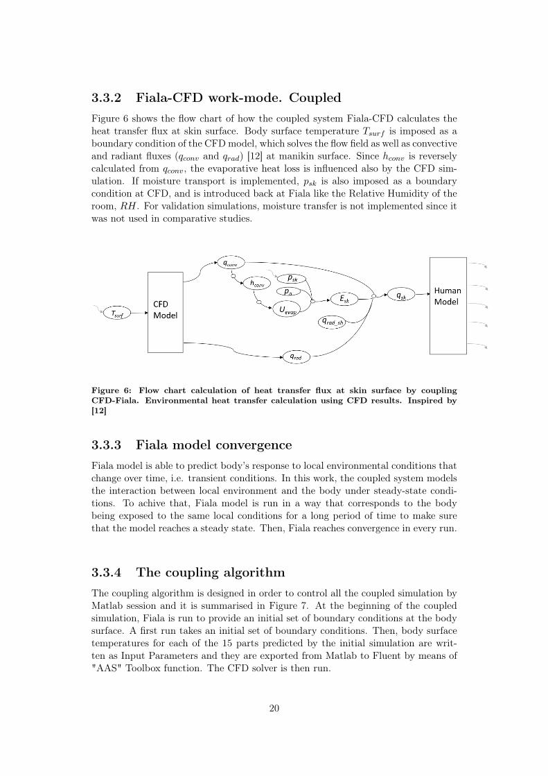
3.3.2 Fiala-CFD work-mode. CoupledFigure 6 shows the flow chart of how the coupled system Fiala-CFD calculates theheat transfer flux at skin surface. Body surface temperature Tsurf is imposed as aboundary condition of the CFDmodel, which solves the flow field as well as convectiveand radiant fluxes (qconv and qrad) [12] at manikin surface. Since hconv is reverselycalculated from qconv, the evaporative heat loss is influenced also by the CFD sim-ulation. If moisture transport is implemented, psk is also imposed as a boundarycondition at CFD, and is introduced back at Fiala like the Relative Humidity of theroom, RH. For validation simulations, moisture transfer is not implemented since itwas not used in comparative studies.
Figure 6: Flow chart calculation of heat transfer flux at skin surface by couplingCFD-Fiala. Environmental heat transfer calculation using CFD results. Inspired by[12]
3.3.3 Fiala model convergenceFiala model is able to predict body’s response to local environmental conditions thatchange over time, i.e. transient conditions. In this work, the coupled system modelsthe interaction between local environment and the body under steady-state condi-tions. To achive that, Fiala model is run in a way that corresponds to the bodybeing exposed to the same local conditions for a long period of time to make surethat the model reaches a steady state. Then, Fiala reaches convergence in every run.
3.3.4 The coupling algorithmThe coupling algorithm is designed in order to control all the coupled simulation byMatlab session and it is summarised in Figure 7. At the beginning of the coupledsimulation, Fiala is run to provide an initial set of boundary conditions at the bodysurface. A first run takes an initial set of boundary conditions. Then, body surfacetemperatures for each of the 15 parts predicted by the initial simulation are writ-ten as Input Parameters and they are exported from Matlab to Fluent by means of"AAS" Toolbox function. The CFD solver is then run.
20
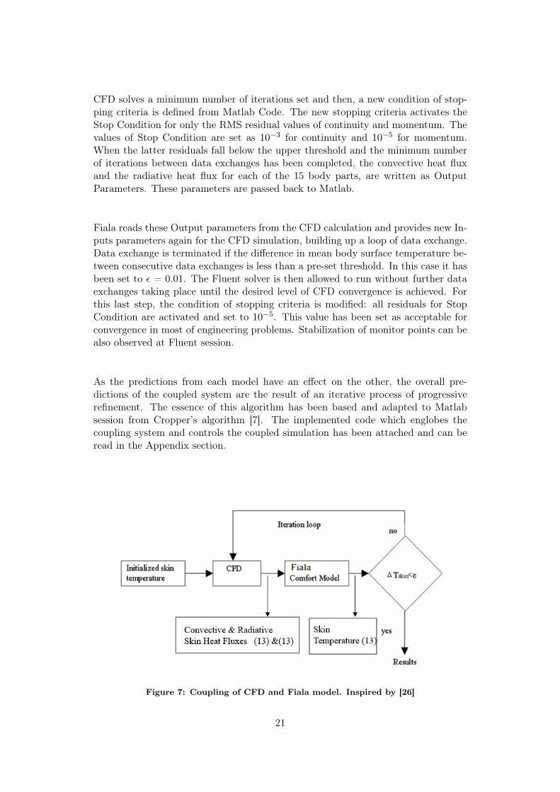
CFD solves a minimum number of iterations set and then, a new condition of stop-ping criteria is defined from Matlab Code. The new stopping criteria activates theStop Condition for only the RMS residual values of continuity and momentum. Thevalues of Stop Condition are set as 10−3 for continuity and 10−5 for momentum.When the latter residuals fall below the upper threshold and the minimum numberof iterations between data exchanges has been completed, the convective heat fluxand the radiative heat flux for each of the 15 body parts, are written as OutputParameters. These parameters are passed back to Matlab.
Fiala reads these Output parameters from the CFD calculation and provides new In-puts parameters again for the CFD simulation, building up a loop of data exchange.Data exchange is terminated if the difference in mean body surface temperature be-tween consecutive data exchanges is less than a pre-set threshold. In this case it hasbeen set to ε = 0.01. The Fluent solver is then allowed to run without further dataexchanges taking place until the desired level of CFD convergence is achieved. Forthis last step, the condition of stopping criteria is modified: all residuals for StopCondition are activated and set to 10−5. This value has been set as acceptable forconvergence in most of engineering problems. Stabilization of monitor points can bealso observed at Fluent session.
As the predictions from each model have an effect on the other, the overall pre-dictions of the coupled system are the result of an iterative process of progressiverefinement. The essence of this algorithm has been based and adapted to Matlabsession from Cropper’s algorithm [7]. The implemented code which englobes thecoupling system and controls the coupled simulation has been attached and can beread in the Appendix section.
Figure 7: Coupling of CFD and Fiala model. Inspired by [26]
21

3.4 CFD Design. Human in a 3D simplifiedRoom
A first simulation was carried out in a simple environment in order to simplify theboundary conditions which could lead to unstabilities in the coupling system. A 3DRoom was decided to be performed to be also validated by similar research works.The commercial CFD code ANSYS Fluent, version 2019 R2, was used to modelairflow and heat transfer. Steady-state simulations have been used to model thethermal conditions in an indoor environment with a human body as the only heatsource.
3.4.1 Computer Aided Model (CAD)
The computational domain has been reproduced from the work done by Cropper[3], [7]. It consists of a box which dimensions of width and depth are 3 m (to omithorizontal aspect ratio effects) and a height of 2.5 m. The domain has four 0.25 mx 0.25 m ventilation openings at floor level and two 0.25 m x 0.25 m openings atceiling level, defined as free openings. This configuration was motivated for havingminimal effect on the thermal plume generated by the human located in the center ofthe room, the only driving force being the metabolic heat generated by the occupant.
The human geometry model is taken from the work done by Raina et. al. [2] andwas conceived to represent a human passenger seated inside an aircraft.
Figure 8: A computational thermal manikin in a naturally ventilated room with upperand lower openings. Inlets in green, outlets in red.
22
3.4.2 Model meshing
The mesh generation process was done in ANSYS Fluent meshing 2019 R2. The firststep in meshing was to create a proper surface mesh. The surface mesh generatedhas a skewness of 0.55 which indicates a good mesh quality. Volume meshing isthen generated with a hexahedral type with an orthogonal quality of 0.36 which alsoindicates a good enough quality of the mesh.
The manikin, which was subdivided into 13 body parts, had a total of 48,948 surfacemesh elements. There were 10 prism layers are placed near manikin body and walls(see Figure 10). The computational domain is composed of approximately 1.1 millionunstructured and structured elements. The body is covered by a body of influenceto set a local mesh sizing of 2 mm.
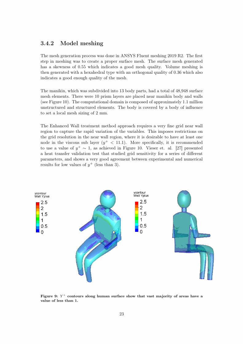
The Enhanced Wall treatment method approach requires a very fine grid near wallregion to capture the rapid variation of the variables. This imposes restrictions onthe grid resolution in the near wall region, where it is desirable to have at least onenode in the viscous sub layer (y+ < 11.1). More specifically, it is recommendedto use a value of y+ ∼ 1, as achieved in Figure 10. Vieser et. al. [27] presenteda heat transfer validation test that studied grid sensitivity for a series of differentparameters, and shows a very good agreement between experimental and numericalresults for low values of y+ (less than 3).
Figure 9: Y + contours along human surface show that vast majority of areas have avalue of less than 1.
23

1
CoordinateX
Co
ord
ina
teY
1 0.5 0 0.5 1 1.50.5
0
0.5
1
1.5
Figure 10: Simplified 3D room mesh using body sizing from body of influence andinflation layer of prisms cells created along human and room wall boundaries.
3.4.3 Physics to solve - Problem modellingDue to the temperature difference between the human body and its surroundings,the airflow pattern close to the body can be a mixed convection flow or a naturalconvection flow which depends on whether the human body is placed in stagnantair or not. The importance of buoyancy forces in a mixed convection flow can bemeasured by the ratio of the Grashof and Reynolds numbers.
Rayleigh numbers less than 108 indicate a buoyancy induced laminar flow, with tran-sition to turbulence occurring over the range of 108 < Ra < 1010. If it is assumedthat the human body to be a cylinder with the height of 1.65m and radius of 0.15m, the Reynolds number will exceed 2500 based on the equivalent diameter of 0.3m as the characteristic length of a human body if the air velocity is more than0.13 m · s−11. When a human body is sitting in stagnant air, the Ra number willreach about 4.1 ·109 at the head level, assuming the temperature difference is 9 oC.Therefore, in most cases the airflow around the human body is turbulent or is in thetransition zone from laminar flow to turbulent flow. However, strictly speaking, thek-epsilon model is only applicable in the fully developed turbulent flow. It is dif-ficult to reproduce the transition from laminar to turbulent with the k-epsilon model.
24

Furthermore, the k-epsilon model is not accurate enough for simulating the air flowfield around a bluff body. Murakami et al. [5] used a contrived method on a k-epsilonmodel to simulate this transition flow by adding a slight turbulence generation termto the k-equation and epsilon-equation throughout the whole computational domain.Since there may be many typical flow elements, such as jet flow, buoyancy drivenflow, laminar flow and potential flow, in the simulation of air flow in a ventilatedroom with a human body, no turbulence model which is now available can deal per-fectly with this complex flow pattern. The k-epsilon model is the best choice for nowamong various turbulence models available in view of its simulation accuracy andcomputational expense. The low Reynolds number k-epsilon model performs betterin the prediction of heat loss from human body while the standard k-epsilon modeland RNG k-epsilon model are sufficient if the emphasis is on airflow field. In thepresented case, there is mainly natural convection. Heat transfer occurs due to heatexchange by free and forced convection with ambient air. These imposed forced con-vective fluxes are to remove part of the metabolic heat produced by the human body.
Heat transfer modes that occur are convection and radiation. Martinho et. al. (2012)[11] developed a study of a human manikin in a standard 3D-room comparing it withexperimental results. The aim was evaluating possible CFD errors and determiningthe contribution of radiation effects. It was concluded that approximately 40 % ofheat transfer in human body was due to radiation (vs. convection). Hence, radiationis considered to be important to be modelled.
3.4.4 Solver setup
As the indoor temperature differences are relatively small, the Boussinesq approxi-mation is used to model the effects of buoyancy. Buoyancy-driven flows inputs are setas "gravity on" and selecting boussinesq approximation. Boussinesq approximationis taken to model a variable density in air properties, as well as, thermal expansioncoefficient is defined for air at room temperature. For the turbulence modelling,(RNG) k-ε was chosen due to its stability and precision of numerical results [15]. Adiscrete ordinates radiation model with rays was used to model radiant heat trans-fer. (Instead of Monte Carlo with 2 million histories, which Zhang [12] pointed outthat gave similar results for a higher computational cost. The additional compu-tational effort is relatively small because the DO model assumes that radiation isemited isotropically from each surface). In problems with localized sources of heat,the Discrete Ordinates model is probably the best suited for computing radiationfor this case, although the DTRM, with a sufficiently large number of rays, is alsoacceptable [20]. Surfaces emissivity is treated as a constant having a value of 0.95for body surface and 0.83 for surrounding surfaces. [16] [17].
Momentum had to be resolved with 1st order upwind discretization scheme due toconvergence problems with 2nd order. The methods to configurate the software andget a solution step-by-step was consulted in the ANSYS MANUAL [20], section"How to Model Natural Convection and Buoyancy Driven Flows" . First, the cal-culations were run with a low Rayleigh (g = 0.098m/s2) and finally with full gravity.
25

The model settings are listed in Table 8.
Table 6: Solver Settings
Equations Discretisationp-v scheme CoupledTurbulence Model RNG K-epsilon with EWTGradient Least squares cell basedPressure Second orderGradient Least squares cell basedMomentum & Turbulence 1st order upwindEnergy 2nd order upwindDiscrete Ordinates 2nd order upwind
3.4.5 Boundary ConditionsThe boundary conditions that model the heat transfer problem are listed in Table 7.
Table 7: Boundary conditions applied
Region Boundary ConditionsInlet Velocity Inlet 0.15 m/s at 21oCOutlet Pressure Outlet 0 PaWall No Slip Wall Fixed Temperature at 21 oCHuman No Slip Wall Tsk from Fiala or 31oC
3.4.6 Validation I: procedure and verification.Two research studies have been used to validate the CFD model developed. First,Sorensen’s simulation [17] has been tried to be reproduced in order to validate theCFD case in a standalone mode, without any connection of HTRM. It was requiredto validate flow and heat transfer behavior around a heat source with a human shape.As soon as the CFD simulation in standalone mode was proved to be validated, asecond validation was required. Cropper’s simulation with a naked person [7] wastried to be reproduced. This simulation already accounted for the validation of theconnection between a HTRM and a CFD case.
For validation of the CFD-uncoupled case, the CFD has been set up with a bound-ary condition of constant temperature in the skin of 31oC, which is the same thanSorensen [17] has considered in his study. To further validate the CFD calculations,these are compared to experimental and numerical results. Experimental PIV mea-surements are provided in Figure 11, which shows the vertical velocity in a verticalplane x = - 0.12m (front view, approximately centred above the head). NumericalCFD results are also compared at whole body level in Figure 12. The agreementis satisfactory between Sorensen’s experimental measurements [17] and this study’sresults.
26

Figure 11: Validation of uncoupled case. Contours of vertical velocity (m/s), frontviewin x = 0.12 (m) (centred near top of head). Left: measured*, right: calculated.∗(Sorensen [17] experimental measurements. (Tsk = 31oC))
Figure 12: Validation of uncoupled case. Distributions of vertical velocity (m/s).Sideview in symmetry-plane (left) and frontview (right) (centred near top of head).Left: Sorensen*, right: calculated. ∗(Sorensen [17] CFD calculations. (Tsk = 31oC))
For the validation of the CFD-coupled case, the CFD has been set up with a bound-ary condition of Fiala skin temperature, which is the same than Cropper [7] hasconsidered in his study. For it, Fiala has been configured in a similar way thanCropper had, that is a naked person. An activity level of 1.2 met has been used as itis the activity level a person would output if seated while reading. The temperatureof the skin of Fiala has been imposed as a boundary condition to predict flow field.
27

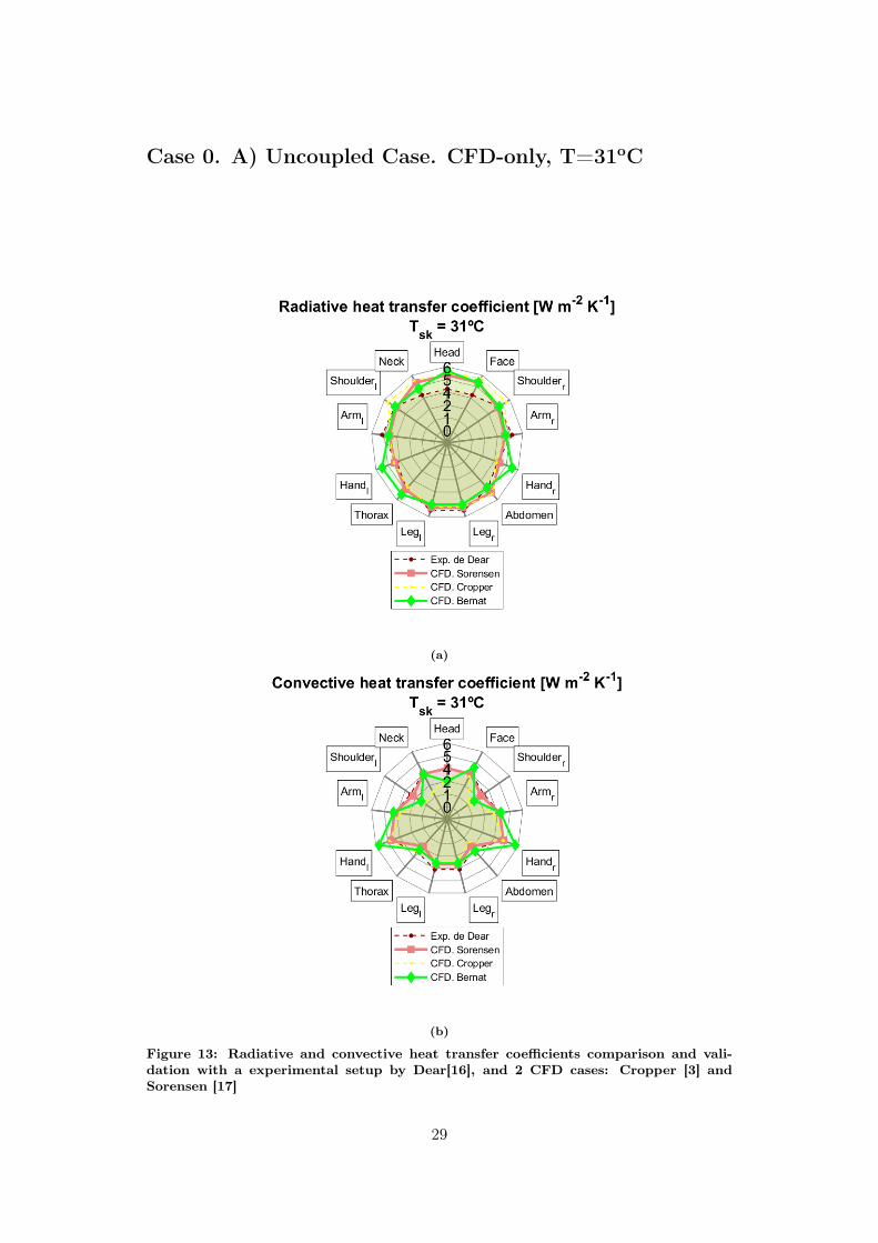
3.4.7 Validation II: Heat transfer coefficientsApart from a qualitative validation of flow contours, a quantitative validation is alsorequired. The surface heat transfer coefficient is the heat flux (convective or radia-tive) divided by the difference between the local wall temperature and the near-wallair temperature. The heat transfer coefficient depicts the transfer of heat from thehuman to the room surrounding. The surface heat transfer coefficient is imple-mented from the available heat transfer variables under the wall fluxes category forpost-processing in ANSYS Fluent. A User Defined Function has been implementedto obtain the convective heat transfer coefficient by dividing the convective heat fluxby the temperature difference between the skin and the near-wall air temperature.The same procedure has been approached to obtain the radiative heat transfer coef-ficient. The near-wall air temperature that has been considered for this study is theroom temperature (21oC), because it is what all authors have taken for reference.The same temperature conditions are required to be able to establish a comparison.
As explained in Section Validation I, two cases are going to be compared: Case 0.A)Uncoupled Case, and Case 0.B) Coupled case. For each of them, radiative and con-vective heat transfer coefficients for each of 13 body parts are going to be comparedwith experimental [16], and other 2 CFD data [7] and [17]. Experimental coefficientswere obtained by de Dear [16] (1997), in which a nude female manikin, whose skintemperature was maintained at a constant temperature, was placed in a test cham-ber. In this experiment, heat transfer coefficients were determined by measuring theenergy required to maintain a constant surface temperature over 16 body regions.The combined heat loss, i.e. the sum of the convective and radiative components, wasfirst determined. Selected areas of the manikin were then covered by a low Emissiv-ity material and the experiment repeated in order to isolate the radiative component.
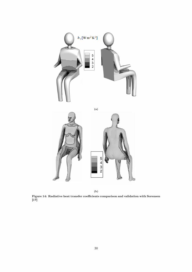
It is expected that Case 0.A) that is the uncoupled case, as shown in Figure 13, CFDBernat (green line) (that is the case of this study) results are more similar to CFDSorensen (pink line), since they both represent a naked seated human with a constanttemperature of T=31oC. Thicker lines were represented to highlight these two datasets. It is expected that Case 0.B) that is the coupled case, as shown in Figure 16,CFD Bernat (green line) results are more similar to CFD Cropper (yellow line), sincethey both represent a naked human with Fiala imposed body temperature. Thickerlines were represented to highlight these two data sets. Due to problems to compareheat transfer coefficients because authors defining different segmentation for bodyparts causing a possible mismatching, body plots have been attached when authors’data was found, in Figures 15b and 14b.
Contour plots of velocity and temperature distributions in the coupled simulationhave also been attached in Figure 17 (bottom). It can be seen that the thermalplume develops over the height of the body and reaches a maximum speed of 0.32 m/sabout 0.5 m above human head. The spatial air temperature distribution and surfacetemperature on the manikin body parts is also shown in Figure 17 (top), where it canbe seen that the coupled system predicts a non-uniform surface temperature withthe head and upper torso predicted to be at a higher temperature than the handsand legs.
28
Case 0. A) Uncoupled Case. CFD-only, T=31oC
(a)
(b)
Figure 13: Radiative and convective heat transfer coefficients comparison and vali-dation with a experimental setup by Dear[16], and 2 CFD cases: Cropper [3] andSorensen [17]
29
(a)
(b)
Figure 14: Radiative heat transfer coefficients comparison and validation with Sorensen[17]
30

(a)
(b)
Figure 15: Radiative heat transfer coefficients comparison and validation with Sorensen[17]
31
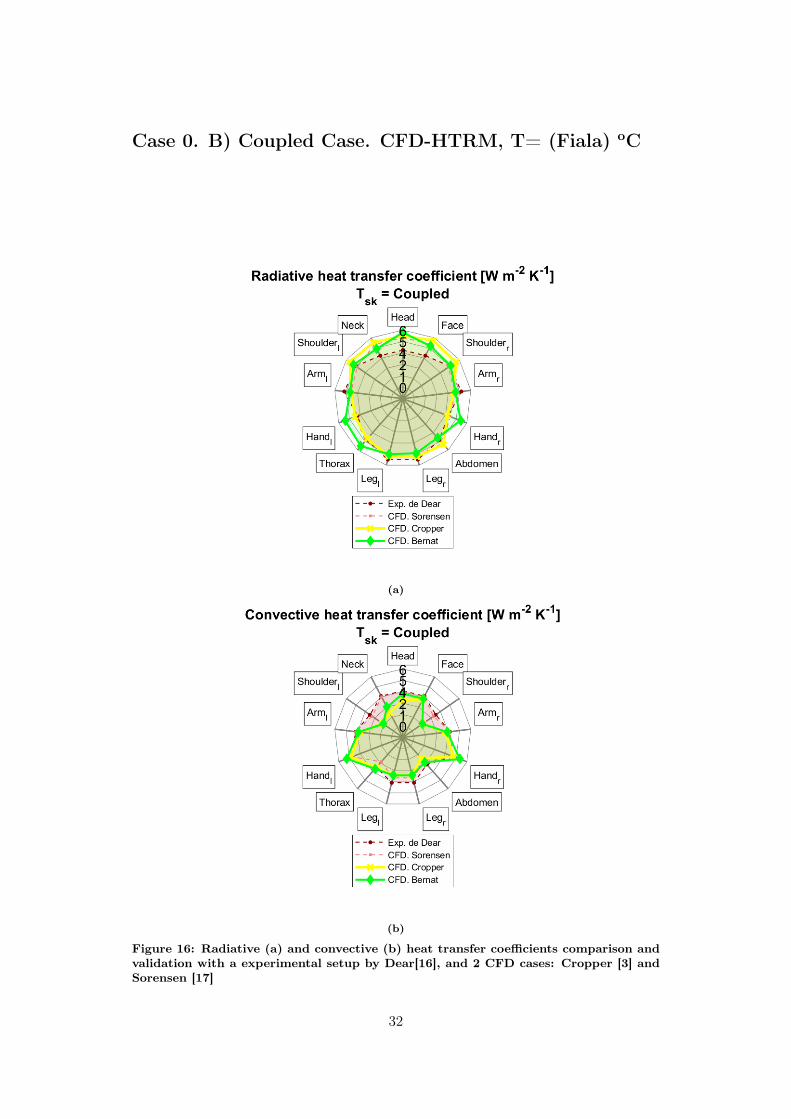
Case 0. B) Coupled Case. CFD-HTRM, T= (Fiala) oC
(a)
(b)
Figure 16: Radiative (a) and convective (b) heat transfer coefficients comparison andvalidation with a experimental setup by Dear[16], and 2 CFD cases: Cropper [3] andSorensen [17]
32

Figure 17: Temperature and velocity contour plots at sections crossing the center ofthe head of the manikin. Coupled simulation.
33

3.5 CFD Design Application. Human in theCabin
The coupling system has been applied to an aircraft cabin model created by Rainaet. al. [2]. It models a single aisle passenger cabin of a regional jet aircraft withhuman manikins as passengers. The inlets and outlets are modelled as strips byapproximating ventilation inlet and outlet average nozzle areas from actual aircraftcabins. Although three different ventilation systems were studied, here displacementventilation configuration (DV) will be coupled to the HTRM. Displacement ventila-tion is probably the best configuration to ensure convergence. That is because theflow is simply going upwards, without any big whirls that may cause instabilities.
3.5.1 CAD Model - Cabin
Figure 18: Displacement Ventilation configuration illustration. [blue arrows indicatefresh air realised from inlet diffuser, red arrows indicate outle for air exraction, yellowarrows depict thermal plumes arising from heat sources.
3.5.2 Human modelThe human model that was used for this simulation was the same than used inAbishek et. al. [2], and that also was used in this thesis for the "Human in the 3DRoom" part.
3.5.3 Model meshingThe mesh generation process was done in ANSYS Fluent meshing 2019 R2. Themesh could have been reused from Abishek et. al. [2] but since it required geometrymodifications in the humans, a replica had to be done manually from scratch. A finermesh is used closer to the human manikins, walls and overhead baggage bin becauseof the larger airflow and temperature gradients that are generated in their vicinity
34

(see Figure 19). The first step in meshing was to create a proper surface mesh. Thesurface mesh generated has a skewness of 0.65 which indicates a good mesh quality.Volume meshing is then generated with a polyhedral type with a maximum skewnessof 0.92 and a minimum orthogonal quality of 0.28 which also indicates a good enoughquality of the mesh.
The manikin was subdivided into 13 body parts. There were 10 prism layers areplaced near manikin body and walls with a smooth transition. Yplus value of lessthan 1 is achieved with a growth ratio of 1.2. The computational domain is composedof approximately 7.7 million unstructured and structured elements. The bodies arecovered by two bodies of influence (BOI) to set a local mesh sizing of 8 mm. Localface meshing is also employed on the walls.
Figure 19: Polyhedral volume mesh with prism layers near walls and two BOI sur-rounding the passengers.
3.5.4 Solver setupSteady state simulations are carried out in ANSYS Fluent 19.2, likewise "Case 0:Human in a 3D room". Pressure based solvers are chosen due to low velocity flowsin the aircraft cabin. The RNG K-epsilon model with Enhanced wall treatment isemployed for turbulence as it was shown to be favoured for indoor flow simulations.The solver setup can be deeply consulted in Abhishek et. al. [2], for the presentthesis only two modifications are carried out. These modifications are: addition ofradiation model and addition of buoyancy forces to the domain.
35

Discrete Ordinates is used to model radiation, and values for Theta and Phi Divi-sions are 3 and Theta and Phi pixels are 2. Increasing the discretization of ThetaDivisions and Phi Divisions to a minimum of 3, will achieve more reliable results. Afiner angular discretization can be specified to better resolve the influence of smallgeometric features or strong spatial variations in temperature. Boussinesq approxi-mation is used to model buoyancy forces in the domain.
Table 8: Solver Settings
Equations Discretisationp-v scheme CoupledTurbulence Model RNG K-epsilon with EWTGradient Least squares cell basedTurbulence 1st order upwindMomentum & Energy 2nd order upwindSpecies 2nd order upwindDiscrete Ordinates 2nd order upwind
3.5.5 Boundary Conditions
A cabin inlet velocity of 0.26 m/s is used for this study based on 50% of the requiredairflow rate per passenger as stated by FAR regulations. 100% of the airflow rate wasnot studied since convergence was not obtained. To achieve the free outflow fromthe domain, a pressure outlet of 0 Pa is set. The cabin wall and seats are assumedas adiabatic, meanwhile the human skin temperature is imposed by whether a fixedtemperature of 31oC or coupled with the HTRM.The boundary conditions that model the heat transfer problem are listed in Table 9.The temperature of the skin is set by the thermoregulatory model when a coupledsimulation is applied.
Table 9: Boundary conditions applied
Region Boundary Conditions DV DV-coupledInlet Velocity Inlet 0.26 m/s 0.26 m/sOutlet Pressure Outlet 0 Pa 0 PaWall Adiabatic Wall - -Human No Slip Wall 31oC Tsk from FialaPeriodic Zone Periodic Interface - -
Case 1 Case 2 & 3
Three different cases have been studied. Case 1 consists of an uncoupled simula-tion with Displacement Ventilation, ’DV’, and a fixed temperature of 31oC for everyhuman. Case 2 consists of a coupled simulation with the right window passengercoupled, ’DV-coupled’. Case 3 consists also of a coupled simulation with both theright aisle and window passengers coupled, ’DV-coupled’.
36
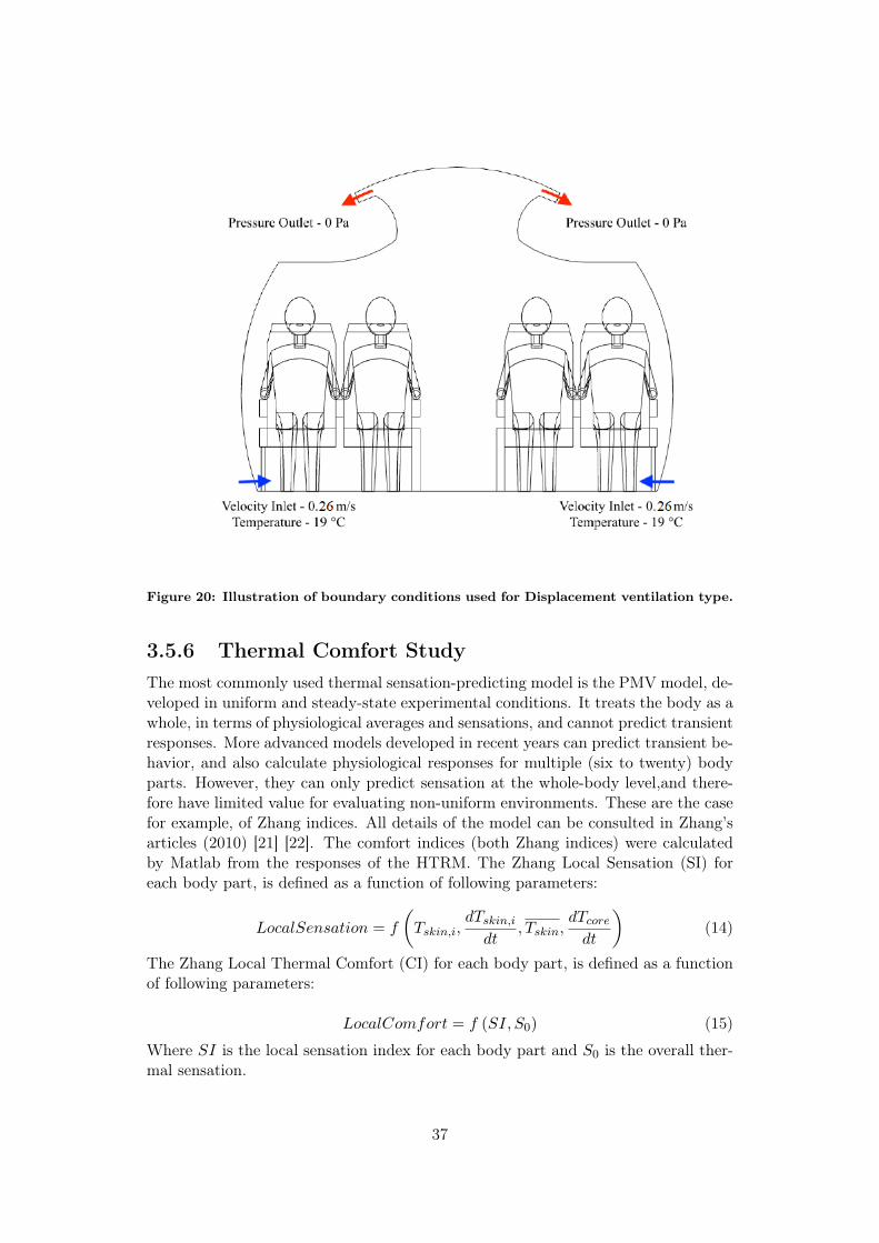
Figure 20: Illustration of boundary conditions used for Displacement ventilation type.
3.5.6 Thermal Comfort StudyThe most commonly used thermal sensation-predicting model is the PMV model, de-veloped in uniform and steady-state experimental conditions. It treats the body as awhole, in terms of physiological averages and sensations, and cannot predict transientresponses. More advanced models developed in recent years can predict transient be-havior, and also calculate physiological responses for multiple (six to twenty) bodyparts. However, they can only predict sensation at the whole-body level,and there-fore have limited value for evaluating non-uniform environments. These are the casefor example, of Zhang indices. All details of the model can be consulted in Zhang’sarticles (2010) [21] [22]. The comfort indices (both Zhang indices) were calculatedby Matlab from the responses of the HTRM. The Zhang Local Sensation (SI) foreach body part, is defined as a function of following parameters:
LocalSensation = f
(Tskin,i,
dTskin,idt
, Tskin,dTcoredt
)(14)
The Zhang Local Thermal Comfort (CI) for each body part, is defined as a functionof following parameters:
LocalComfort = f (SI, S0) (15)
Where SI is the local sensation index for each body part and S0 is the overall ther-mal sensation.
37
3.5.7 Calculation of Neutral skin temperature set points,Tskset
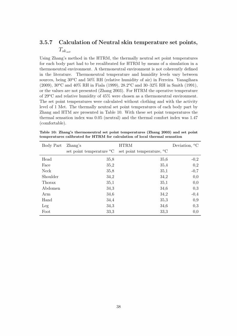
Using Zhang’s method in the HTRM, the thermally neutral set point temperaturesfor each body part had to be recalibrated for HTRM by means of a simulation in athermoneutral environment. A thermoneutral environment is not coherently definedin the literature. Thermoneutral temperature and humidity levels vary betweensources, being 30oC and 50% RH (relative humidity of air) in Ferreira Yanagihara(2009), 30oC and 40% RH in Fiala (1999), 28.2oC and 30–32% RH in Smith (1991),or the values are not presented (Zhang 2003). For HTRM the operative temperatureof 29oC and relative humidity of 45% were chosen as a thermoneutral environment.The set point temperatures were calculated without clothing and with the activitylevel of 1 Met. The thermally neutral set point temperatures of each body part byZhang and HTM are presented in Table 10. With these set point temperatures thethermal sensation index was 0.05 (neutral) and the thermal comfort index was 1.47(comfortable).
Table 10: Zhang’s thermoneutral set point temperatures (Zhang 2003) and set pointtemperatures calibrated for HTRM for calculation of local thermal sensation
Body Part Zhang’s HTRM Deviation, oCset point temperature oC set point temperature, oC
Head 35,8 35,6 -0,2Face 35,2 35,4 0,2Neck 35,8 35,1 -0,7Shoulder 34,2 34,2 0,0Thorax 35,1 35,1 0,0Abdomen 34,3 34,6 0,3Arm 34,6 34,2 -0,4Hand 34,4 35,3 0,9Leg 34,3 34,6 0,3Foot 33,3 33,3 0,0
38

4 Results
4.1 Velocity Distribution in the Cabin with Hu-mans
Figure 21 displays the magnitude of velocity fields revealing that natural convectioninduced by humans is prevailing over forced convection from the inlet. Passengersconnected to a HTRM display an "X-HTRM" mark. Symmetry in the flow is visiblefor the uncoupled case, Case 1, where the humans have all the same temperature.Case 2 breaks the symmetry of Case 1, due to the human coupled with HTRM thatis a bit colder than the other ones, having an average skin temperature of 27.74oC.Case 3 is not as symmetric as Case 1, but humans (window and aisle) have a similaraverage skin temperature of 29.18oC and 29.16oC respectively.
(a) Case 1. Uncoupled - Tsk = 31oC (b) Case 2. Coupled. 1 person - Tsk = Fiala
(c) Case 3. Coupled. 2 people - Tsk = Fiala
Figure 21: Velocity contour plots for different couplings
39
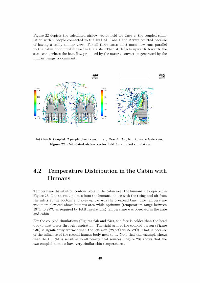
Figure 22 depicts the calculated airflow vector field for Case 3, the coupled simu-lation with 2 people connected to the HTRM. Case 1 and 2 were omitted becauseof having a really similar view. For all three cases, inlet mass flow runs parallelto the cabin floor until it reaches the aisle. Then it deflects upwards towards theseats zone, where the heat flow produced by the natural convection generated by thehuman beings is dominant.
(a) Case 3. Coupled. 2 people (front view) (b) Case 3. Coupled. 2 people (side view)
Figure 22: Calculated airflow vector field for coupled simulation
4.2 Temperature Distribution in the Cabin withHumans
Temperature distribution contour plots in the cabin near the humans are depicted inFigure 23. The thermal plumes from the humans induce with the rising cool air fromthe inlets at the bottom and rises up towards the overhead bins. The temperaturewas more elevated above humans area while optimum (temperature range between19oC to 27oC as required by FAR regulations) temperature was observed in the aisleand cabin.
For the coupled simulations (Figures 23b and 23c), the face is colder than the headdue to heat losses through respiration. The right arm of the coupled person (Figure23b) is significantly warmer than the left arm (28.8oC vs 27.7oC). That is becauseof the influence of the second human body next to it. Note that this example showsthat the HTRM is sensitive to all nearby heat sources. Figure 23a shows that thetwo coupled humans have very similar skin temperatures.
40

(a) Case 1. Uncoupled - Tsk = 31oC (b) Case 2. Coupled. 1 person - Tsk = Fiala
(c) Case 3. Coupled. 2 people - Tsk = Fiala
Figure 23: Temperature contour plots for different couplings
4.3 Heat Transfer Coefficient on Humans for dif-ferent couplings
The surface heat transfer coefficient is the heat flux divided by the difference be-tween the local wall temperature and the sorrounding air temperature. The heattransfer coefficient in all the three different coupling scenarios depicts the transferof heat from the human to the cabin surrounding. The surface heat transfer co-efficient is implemented as a User Defined Function in ANSYS Fluent, in order tohave separately the radiative and the convective heat transfer coefficients. Theseparameters are iterated by means of heat fluxes until a balance is found betweenexchanges. Figure 24 show convective surface heat transfer coefficient (left side -Figures 24a,24c,24e) and radiative heat transfer coefficient (right side - Figures 24b,24d, 24f) for the different couplings. For all of them, passengers experience a lowheat transfer coefficient range overall, highest convective heat transfer coefficient isgiven on the lower legs, where the velocity is higher due to bottom located inletdiffusers. Figure 24a and 24b show symmetry in both radiative and convective heattransfer coefficients for the uncoupled case.
41

(a) Case 1. Uncoupled - Tsk = 31oC (b) Case 1. Uncoupled - Tsk = 31oC
(c) Case 2. Coupled. 1 person - Tsk = Fiala (d) Case 2. Coupled. 1 person - Tsk = Fiala
(e) Case 3. Coupled. 2 people - Tsk = Fiala (f) Case 3. Coupled. 2 people - Tsk = Fiala
Figure 24: Convective (a, c & e) & Radiative (b, d & f) heat transfer coefficient fordifferent couplings
42

4.4 Thermal Comfort StudyFigure 25 depicts both the Thermal Sensation Index (left) and the Thermal Com-fort Index (right) for the three simulated cases. These results were obtained usingZhang’s thermal comfort approach (2010) which has been explained in the Theorysection and detailed in the Method section. From these Figures implemented inMatlab, an approach of both quantitative and qualitative comfort is displayed. ’LS -1 Person WD’ corresponds to the Local Sensation for the coupled simulation of only1 person, which is sitting by the window. ’LS - 2 Person WD’ corresponds to thecoupled simulation of 2 people, and in this case the person analyzed is the personsitting by the window. ’LS - 2 Person AI’ corresponds to the latter case but now theperson sitting by the aisle is analyzed.
The resulting sensation scale ranges and comfort index ranges can be consulted inTables 4 and 5 respectively.
Figure 25: Predicted distribution of the Zhang Sensation and the Local Comfort indiceson the passengers in a row of the cabin
43
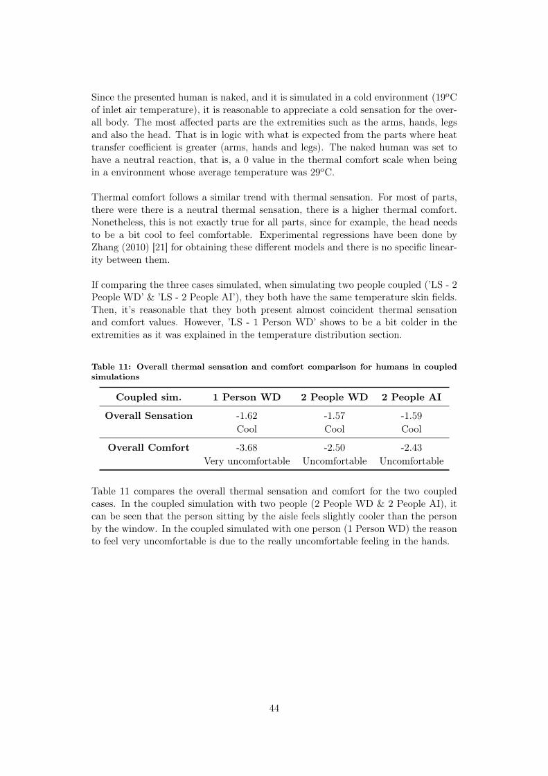
Since the presented human is naked, and it is simulated in a cold environment (19oCof inlet air temperature), it is reasonable to appreciate a cold sensation for the over-all body. The most affected parts are the extremities such as the arms, hands, legsand also the head. That is in logic with what is expected from the parts where heattransfer coefficient is greater (arms, hands and legs). The naked human was set tohave a neutral reaction, that is, a 0 value in the thermal comfort scale when beingin a environment whose average temperature was 29oC.
Thermal comfort follows a similar trend with thermal sensation. For most of parts,there were there is a neutral thermal sensation, there is a higher thermal comfort.Nonetheless, this is not exactly true for all parts, since for example, the head needsto be a bit cool to feel comfortable. Experimental regressions have been done byZhang (2010) [21] for obtaining these different models and there is no specific linear-ity between them.
If comparing the three cases simulated, when simulating two people coupled (’LS - 2People WD’ & ’LS - 2 People AI’), they both have the same temperature skin fields.Then, it’s reasonable that they both present almost coincident thermal sensationand comfort values. However, ’LS - 1 Person WD’ shows to be a bit colder in theextremities as it was explained in the temperature distribution section.
Table 11: Overall thermal sensation and comfort comparison for humans in coupledsimulations
Coupled sim. 1 Person WD 2 People WD 2 People AI
Overall Sensation -1.62 -1.57 -1.59Cool Cool Cool
Overall Comfort -3.68 -2.50 -2.43Very uncomfortable Uncomfortable Uncomfortable
Table 11 compares the overall thermal sensation and comfort for the two coupledcases. In the coupled simulation with two people (2 People WD & 2 People AI), itcan be seen that the person sitting by the aisle feels slightly cooler than the personby the window. In the coupled simulated with one person (1 Person WD) the reasonto feel very uncomfortable is due to the really uncomfortable feeling in the hands.
44
5 DiscussionHuman in a 3D Room5.1 Validation
Heat transfer coefficients comparison
5.1.1 Case 0. A) Uncoupled Case.There are some differences in the methods of every author that lead to minor disagree-ments in the results. These are going to be explained thoroughly. The experimentalmanikin considered by De Dear [16] is wigged with shoulder-length hair, whereas theComputational manikin is bald for all CFD simulations (Sorensen) [17], (Cropper)[7]. For the head of the manikin, this probably explains the larger radiative heattransfer coefficient of the calculation compared to the measurements, as it can beseen in Figures 13b and 16b. This is also believed to explain the larger calculatedvalue for the radiative heat transfer for the back of the manikin. It should be takeninto account that no real humans were tested by neither De Dear, nor Sorensen norCropper, but all they used manikins.
Major differences for heat transfer coefficient are in the hands. This fact is due tothe undevelopment of this body part, since hands are taken only as a slice of theend of the arm. If they were further developed, a good agreement may be achieved.Foot were not considered since the geometry didn’t allow it.
Minor differences occur for the "head-face-neck" group, and this is because every au-thor has separated the body in different body parts that don’t really match. Sorensenand de Dear took the head in global as the head, face and neck. Meanwhile in thisstudy, the head is only the section that would be protecting brain area. Face isalso separated, as well as the neck. Sorensen and de Dear have a similar separationbecause they were using only a manikin model, regardless the inner body heat phe-nomena. Nevertheless, as soon as it is desired to couple a thermoregulatory model,the discretization of the body in CFD comes imposed by the number of parts thathas the thermoregulatory model. That’s why the present model is discretized simi-larly than Cropper, although with less body parts (13). Cropper had 59 body partsbecause a further developed Fiala model - IESDFiala - was used instead.
The same fact happens for the shoulders, Sorensen and de Dear called "shoulders"to the upper arm. It is translated into a higher value of convective heat transfercoefficient visible in the spider chart (see Figure 13a) for this part. For that, plots ofthe convective heat transfer coefficients on the body surface were plot intentionallyto correct different parts spelling errors. Comparing Figures 15b and 15a, shouldersvalue match.
45

5.1.2 Case 0. A) Coupled Case.Differences between the coupled simulation stay in the differences between Crop-per and this study model, that basically is that Cropper is at standing position,meanwhile this study model is seating. It explains that this model achieves a lowerradiative heat transfer coefficient (See Figure 16b). Since the flow is going fromlegs to head direction (going upwards), when the manikin is seated the legs makea "shadow" effect to the abdomen (see Figure 15) resulting in a decreasement ofradiative heat transfer coefficient. This also has a decreasement in convective heattransfer coefficient, since the legs are blocking part of the flow that comes upwards.Moreover, Cropper results were given in 59 values of body parts that had to bematched to get a similar discretization to this study, which also introduces error.
Both, for the coupled and the uncoupled case, the heat transfer coefficients evaluatedat whole body level agree satisfactorily with other CFD simulations and experimen-tal data. An average value of 4.9 [W ·m2 ·K−1] for radiant heat transfer coefficientand for convective heat transfer coefficient 3.1 [W ·m2 ·K−1] are obtained. As it canbe checked in the Tables 12 and 13 in the Appendix section.
Human in the Cabin5.2 MethodologyThe major new scientific knowledge of this thesis is combining the human thermalmodelling with a thermal sensation and comfort model inside of a CFD simulationprogram. This approach enables i) calculating more realistically the interaction andnon uniform transient heat transfer between the skin surface and the surrounding airand building structures and ii) taking into account the effect of human thermoregu-lation and individual human parameters on thermal sensation and comfort.
The coupled model presents inherent limitations which condition that it cannot becompared with experimental results such as photographs of the cabin taken by ther-mography. Naked humans are the reason for this fact, instead of having clothed ones.The shortage of time and being out of the scope of this thesis argue this reason. Sub-sequently, as soon as the cloth model is implemented in the HTRM, comparisons oftemperature plots with experimental results will be available.
CFD model had to be run with 50% of the ventilation, not accomplishing FAR reg-ulations, due to problems with convergence. It was taken as a measure to prioritizehaving the coupled model up and running. Probably the lack of convergence wasdue to a need for a higher mesh density in the aisle region (out of CPU capacity,being 13 million cells the maximum applicable). The mesh used was a replica fromthe mesh provided by Abishek and Raina [2] whose results proved to be mesh inde-pendent. Nonetheless, when applying Boussinesq model and activating subsequentlynatural convection, this mesh seemed to have trouble when modeling more chal-
46
lenging environments with higher ventilation. For every simulation, CPU time wasintensive. Running the uncoupled simulation took 72h and the coupled simulationstook around 5-6 days. 12 consecutive exchanges between Matlab and CFD were re-quired till convergence was achieved. This fact also contributed to a higher difficultyif the mesh was wanted to be improved.
5.3 Thermal Comfort StudyThe approach adopted for Thermal Comfort study, created by Zhang, presents animprovement over the PMV method. The commonly used Fanger’s PMV methodfor thermal sensation and thermal comfort calculation takes into account the averageoperative temperature as a function of the indoor and average surface temperatures.It does not pay attention to the fact that the surface temperatures vary inside of aroom, e.g. during the winter the heating devices are warmer and window surfacescolder than other surfaces. This uneven surface temperature distribution can causethermal discomfort even though the average surface temperature might be accept-able.
Fanger’s PMV method is a heat balance model, which views the human being asa passive recipient of thermal stimuli, assuming that the effects of the surroundingenvironment are explained only by the physics of heat and mass exchanges betweenthe body and the environment, and neglecting the human thermoregulation system.The HTRM method takes into account the human tissue distribution and thermoreg-ulation system in calculation of the skin and core temperatures, their change in timeand the resulting local and overall thermal sensation and thermal comfort. Previousresearch has shown that Fanger’s PMV method is valid for everyday prediction ofthe comfort vote only under severely restricted conditions, because it progressivelyoverestimates the mean perceived warmth of warmer environments and the coolnessof cooler environments.
Zhang’s Method that was used in this thesis, has been successfully validated undervarious steady-state and transient indoor environment boundary conditions extract-ing the numerical regressions of the model from measurements made with real humanbeings.
5.4 ResultsDisplacement Ventilation was observed to be particularly causing human uncom-fortabilities near inlet diffusers located at the bottom. Convective heat transfercoefficient was more elevated near the lower legs and also lower arms and a bit of thehead for the latter reason. Adding to this the effect of also more elevated radiativeheat transfer coefficient for the same parts due to surface to surface radiation, itcaused a lower local skin temperature and consequently a colder thermal sensation.Expected cool sensations were obtained for a naked person due to being in a slightlycool environment (19oC). Probably if a dressed manikin was tested, more comfort-able sensations would be obtained.
47

5.5 Future workFor future work, some developments may be addressed in the scope of this thesis.
On the one hand, the HTRM could be further developed by adding different typeof clothes. In this way, thermal comfort in different environments could be studied,such as which is the impact of cold/hot environments with several clothes. Validationshould be taken into account, and there is the possibility to validate it with IESD-Fiala, easily accessible by the website created by Dr. Zhang ("http://www.jeplus.org/").Hence, comparison with experimental thermography could be evaluated. After hav-ing this achieved, these clothes could be also modeled in the CAD of the humanthat is represented in the CFD model. The effect of simulating a naked human pro-duces overestimating heat losses through convection and showing not real life results.
On the other hand, the CFD model could be tested with different ventilation types,such as mixed or personalized ventilation. The reader should keep in mind the com-plexity when modeling these challenging environments with strong whirls created byforced convection and also buoyancy effects dominating.
Moisture transfer could be also incorporated to the coupled simulation. If the cabinin CFD is decided to be wet, human sweating mass transfer can be incorporated intoCFD as a source of moisture which modifies the relative humidity in the environ-ment. Cropper [3] provides more details about how to do it.
Even though the current version of the Human Thermoregulatory Model, HTRMhas some restrictions and the planned improvements will further develop the model,the current version has been shown in this thesis to estimate accurately enough thethermal sensation and thermal comfort of the human and the HTRM method is amajor improvement to the currently used Fanger’s PMV model.
A comparison study for a steady simulation could be carried out in order to appreci-ate the difference between a coupled simulation with several exchanges and a linearcoupled simulation. A linear coupled simulation means that first the CFD case isconverged with an initial set of skin temperatures and CFD output is directly passedto the HTRM. It would give directly a response of thermal comfort as it was the firstiteration or the first exchange. Note that some errors will occur due to dismissingsome of the effects of the interaction between the environment and the human body,but the study of this error may be of interest to save CPU time.
48

6 ConclusionsThe main objective of this master thesis has been achieved. A coupled simulationtechnique has been developed that enables a multi-segmented model of human ther-mal comfort and physiology to exchange data with a commercial CFD program calledAnsys Fluent. Initially it was developed for a 3DRoom and it was finally applied tothe passengers of an Aircraft Cabin where Displacement ventilation was studied.
The presented numerical thermal comfort predictions are based on the solution ofthe Reynolds-averaged Navier-Stokes equation using the Boussinesq approximationand modeling of surface to surface thermal radiation in an aircraft cabin and a 3Droom, and the coupling with the finite element code HTRM in Matlab. The lat-ter allows to simulate the heat transport within the passengers and the perceivedtemperature and comfort of passengers. The way that the coupling algorithm hasbeen programmed, makes possible that both steady and transient simulations can bestudied. These transient effects will also be taken into account even for the thermalcomfort study.
Comparisons of the predictions for 3D room by the coupled system with publishedexperimental data and previous CFD studies show favourable agreement on the over-all whole body mean heat transfer coefficients in still air conditions. The differencesthat can be observed in some body parts are suspected to be due, in part, differ-ences in surface area between the computational manikin used in this study, andthe experimental nude female manikin and posture. The comparisons described sofar represent a relative simple case, in which the manikin is placed in an initiallyuniform environment. In the next step, Case 1: Human in an aircraft cabin, theresponses of the coupled system to more challenging and non-uniform environmentsare investigated.
Regarding the aircraft cabin, the only objective that was not achieved was analyzingdifferent ventilation systems, due to the high complexity for achieving convergencewhen running CFD cases such as mixing or personalized ventilation. In order tocompensate this lack, a newly improved thermal comfort model was integrated inHTRM. The advantages over traditional traditional Fanger’s PMV are, on the onehand the high range of environmental applications: non-uniform and transient en-vironments are applicable, and also, having local and global parameters to studycomfort for each of the body parts. It was shown that with the presented approacha qualitative and quantitative thermal comfort prediction is possible.
Thermal sensation and comfort results fit to the expected tendencies due to thesimulated thermal environment. In the considered ventilation configuration, maindrawbacks of thermal comfort for the passengers have been identified: draft risk atoutward pointing the legs, arms and hands. The predicted discomfort due to draftrisk at the hands and legs is furthermore intensified by a cold local thermal comfort.
49


References[1] Espuna JC. Development of a Human Thermoregulatory Model for Aviation
Related Application. 1st ed. LiU; 2019.
[2] Raina A, Venkatesan LS. CFD Study on Different Aircraft Cabin VentilationSystems. 1st ed. LiU; 2020.
[3] Cropper PC, Yang T, Cook M, Fiala D, Yousaf R. Coupling a model ofhuman thermoregulation with computational fluid dynamics for predictinghuman–environment interaction. 2010;Available from: https://doi.org/10.1080/19401491003615669/.
[4] Short CA, Shujian N, Weng W. Design guidance for naturally ventilated the-atres. 2005;.
[5] Murakami S, Kato S, Zeng J. Combined simulation of airow, radiation andmoisture transport for heat release from a human body. 1999;.
[6] Al-Mogbel A. A Coupled Model for Predicting Heat and Mass Transfer from aHuman Body to its Surroundings. 2003;.
[7] Cropper PC, Yang T, Cook M, Fiala D. Exchange of simulation data be- tweenCFD programmes and a multisegmented human thermal comfort model.;.
[8] Fiala D, Bunzl A, Lomas KJ, Cropper PC, Schlenz D. A New Simulation Systemfor Predicting Human Thermal and Perceptual Responses in Vehicles. 2004;.
[9] Dixit A, Gade U. A case study on human bio-heat transfer and thermal comfortwithin CFD. 2015;.
[10] Inc A. ANSYS Fluent UDF Manual. ANSYS Inc.; 2013.
[11] Martinho N, Lopes A, da Silva MG. Evaluation of errors on the CFD compu-tation of air flow and heat transfer around the human body. 2012;.
[12] Zhang Y, Yang T. Simulation of human thermal responses in a confined space.2008;.
[13] Yang J, Cook MJ. Modelling heat transfer and physiological responses of un-clothed human body in hot environment by coupling CFD simulation with ther-mal model. 2017;.
[14] Murakami S, Kato S, Zeng J. Flow and temperature fields around humanbody with various room air distributions: CFD study on computational thermalmanikin—Part I. 1997;.
[15] Gao N, Niu J, Zhang H. CFD Study of the Thermal Environment around aHuman Body: A Review. 2005;.
[16] de Dear R, Arens E, Oguro ZHM. Convective and radiative heat transfer coef-ficients for individual human body segments.;.
51
[17] Sorensen D, Voigt L. Modelling flow and heat transfer around a seated humanbody by computational fluid dynamics. 2002;.
[18] Treeck CV, Frish J, Pfaffinger M, Rank E, S Paule IS, Schwab R. Integratedthermal comfort analysis using a parametric manikin model fr interactive real-time simulation. 2009;.
[19] Fiala D. Dynamic Simulation of Human Heat Transfer and Thermal Comfort.PhD thesis. 1999;.
[20] Inc A. ANSYS Fluent Users Guide. ANSYS Inc.; 2013.
[21] Zhang H, Arens E, Huizenga C, Han T. Thermal sensation and comfort modelsfor non-uniform and transient environments: Part I: Local sensation of individ-ual body parts.;.
[22] Zhang H, Arens E, Huizenga C, Han T. Thermal sensation and comfort modelsfor non-uniform and transient environments: Part I: Local comfrt of individualbody parts.;.
[23] ANSYS I. ANSYS as a Server Example: MATLAB Setup. Release 2019 R1,January;.
[24] ANSYS I. ANSYS Fluent as a Server User’s Guide. Release 15.0, November;.
[25] Tanabe S, Kobayashi K, Nakano J, Ozeki Y, Konishi M. Evaluation of ther-mal comfort using combined multi-node thermoregulation (65MN) and radiationmodels and computational fluid dynamics (CFD). 2002;.
[26] Gao N, Niu J, Zhang H. Coupling CFD and Human Bodt ThermoregulationModel for the Assessment of Personalized Ventilation . 2006;.
[27] Nielsen P, Murakami S, Kato S, Topp C. Benchmark tests for a computersimulated person. ISSN 1395-7953 R0307. 2003;.
52
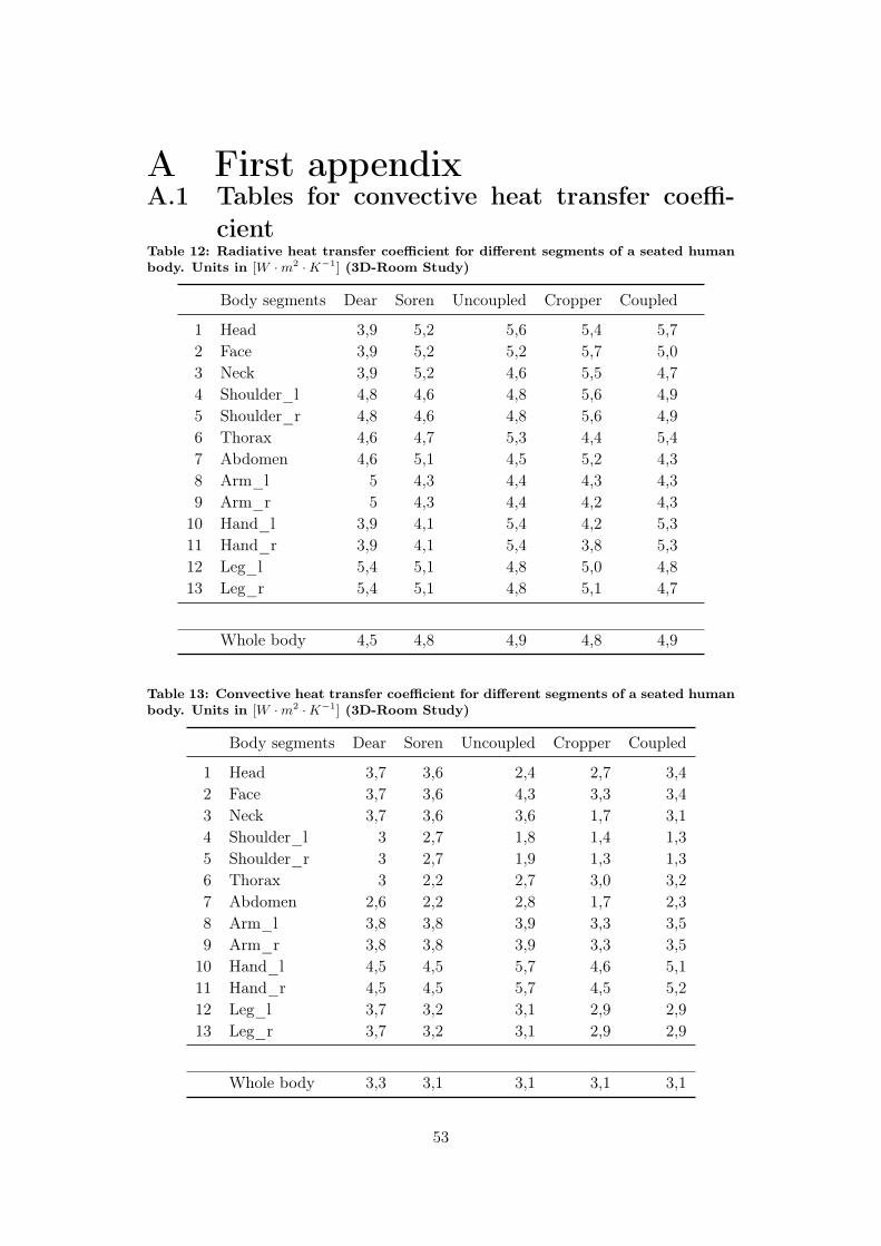
A First appendixA.1 Tables for convective heat transfer coeffi-
cientTable 12: Radiative heat transfer coefficient for different segments of a seated humanbody. Units in [W ·m2 ·K−1] (3D-Room Study)
Body segments Dear Soren Uncoupled Cropper Coupled
1 Head 3,9 5,2 5,6 5,4 5,72 Face 3,9 5,2 5,2 5,7 5,03 Neck 3,9 5,2 4,6 5,5 4,74 Shoulder_l 4,8 4,6 4,8 5,6 4,95 Shoulder_r 4,8 4,6 4,8 5,6 4,96 Thorax 4,6 4,7 5,3 4,4 5,47 Abdomen 4,6 5,1 4,5 5,2 4,38 Arm_l 5 4,3 4,4 4,3 4,39 Arm_r 5 4,3 4,4 4,2 4,310 Hand_l 3,9 4,1 5,4 4,2 5,311 Hand_r 3,9 4,1 5,4 3,8 5,312 Leg_l 5,4 5,1 4,8 5,0 4,813 Leg_r 5,4 5,1 4,8 5,1 4,7
Whole body 4,5 4,8 4,9 4,8 4,9
Table 13: Convective heat transfer coefficient for different segments of a seated humanbody. Units in [W ·m2 ·K−1] (3D-Room Study)
Body segments Dear Soren Uncoupled Cropper Coupled
1 Head 3,7 3,6 2,4 2,7 3,42 Face 3,7 3,6 4,3 3,3 3,43 Neck 3,7 3,6 3,6 1,7 3,14 Shoulder_l 3 2,7 1,8 1,4 1,35 Shoulder_r 3 2,7 1,9 1,3 1,36 Thorax 3 2,2 2,7 3,0 3,27 Abdomen 2,6 2,2 2,8 1,7 2,38 Arm_l 3,8 3,8 3,9 3,3 3,59 Arm_r 3,8 3,8 3,9 3,3 3,510 Hand_l 4,5 4,5 5,7 4,6 5,111 Hand_r 4,5 4,5 5,7 4,5 5,212 Leg_l 3,7 3,2 3,1 2,9 2,913 Leg_r 3,7 3,2 3,1 2,9 2,9
Whole body 3,3 3,1 3,1 3,1 3,1
53

A.2 Manikin body part segmentation
Figure 26: Different human manikins with segmentation of body parts for each studyconsidered to be compared in this report.
A.3 CodeIn this section, two Matlab listings are included: the coupling script that controlsthe Matlab-CFD simulation and the function of Writing Output Parameters.
1 %%% WARNINGS THINGS TO DO:
3 %%% Cautions to run the PROGRAM: to have a l l F i l e s toge the r :%%% 1) aas_Fluent Connections
5 %%% 2) ’ HTRMFighter_function_onlyh .m’%%% 3) FLUENT Direc to ry \\ OR \\ Connect by code with FLUENT Direc to ry
7
%%%% Launch Fluent in Standalone Mode . AAS = 1 . ( See Manual FluentUsers
9 %%%% as a Server Guide ) .%
11 % Modif ied l a s t time 06/06/2020 19 :07%
13 %%%%%%%%%%%%%%%%%%%%%%%%%%%%%%%%%%%%%%%%
15
%% Basic Connection %%%% RUN THIS SECTION Once per s e s s i o n17
orb=i n i t i a l i z e_o r b ( ) ; %i n i t i a l i z e aaS19 load_ansys_aas ( ) ;
f l u e n t=a c t f l u e n t s e r v e r ( orb , ’ aaS_FluentId . txt ’ ) ; %connect to ANSYSproducts
54

21 t u i=f l u e n t . ge tSchemeContro l l e r Ins tance ( ) ;t u i . doMenuCommandToString ( ’ r epo r t summary ’ )
23 %actwbserver ( ’ aaS_WbId . txt ’ ) %To connect Matlab with WorkBench
25 %tu i . doMenuCommandToString ( ’ d e f i n e operat ing cond i t i on s g rav i ty yes 9 . 80 .0 0 . 0 ’ ) ;
27 %% Read the case %%%%%tu i . doMenuCommand( ’ f i l e read case \"C:\ myfo lders \ f ln tgz123604 . cas \" ’ )
29 t u i . doMenuCommand( ’ f i l e read case \"//ad . l i u . se /coop/ i / IEI MVS Thes i s /Marco and Eva/3DROOM/StandaloneFluent /Case&Data/FLTG 1 4 1 rcoupled .cas . gz \" ’ )
t u i . doMenuCommand( ’ f i l e read data \"//ad . l i u . se /coop/ i / IEI MVS Thes i s /Marco and Eva/3DROOM/StandaloneFluent /Case&Data/FLTG 1 4 1 rcoupled .dat . gz \" ’ )
31
%%%%%%%%%%%%%%%%%%%%%%%%%%%%%%%%%%%%%%%%%%%%%%%%%%%%%%%%%%%%%%%%%33 % RUNNING COUPLING PROCESS %%
35 e lements = 15 ; % Number o f Body Part ; %Feet excludedelements_CFD = 13 ;
37 e r r o r = 1 ;exchange = 0 ;
39
% %%I n i t i a l i z a t i o n o f output v a r i a b l e s :41
q_conv_CFD = ze ro s ( elements , 1 ) ;43 q_tot_CFD = ze ro s ( elements , 1 ) ;
q_rad_CFD = ze ro s ( elements , 1 ) ;45 h_conv_CFD = ze ro s ( elements , 1 ) ;
h_rad_CFD = ze ro s ( elements , 1 ) ;47
49
input_T = { ’T_head ’ , ’ T_face ’ , ’T_neck ’ , ’ T_shoulder_l ’ ,’ T_shoulder_r ’ , . . .
51 ’ T_thorax ’ , ’T_abdomen ’ , ’T_arm_l ’ , ’T_arm_r ’ , ’T_hand_l ’ , ’T_hand_r ’ , . . .
’ T_leg_l ’ , ’T_leg_r ’ , ’ T_feet_l ’ , ’ T_feet_r ’ } ’ ;53
output_q_tot = { ’ q_tot_head ’ , ’ q_tot_face ’ ,’ q_tot_neck ’ , ’ q_tot_shoulder_l ’ ,
’ q_tot_shoulder_r ’ , . . .55 ’ q_tot_thorax ’ , ’ q_tot_abdomen ’ , ’
q_tot_arm_l ’ , ’ q_tot_arm_r ’ , ’ q_tot_hand_l ’ , ’ q_tot_hand_r ’ , . . .’ q_tot_leg_l ’ , ’ q_tot_leg_r ’ , ’
q_tot_feet_l ’ , ’ q_tot_feet_r ’ } ’ ;57 output_q_rad = { ’ q_rad_head ’ , ’ q_rad_face ’ ,
’ q_rad_neck ’ , ’ q_rad_shoulder_l ’ , ’ q_rad_shoulder_r’ , . . .
’ q_rad_thorax ’ , ’ q_rad_abdomen ’ , ’q_rad_arm_l ’ , ’q_rad_arm_r ’ , ’ q_rad_hand_l ’ , ’ q_rad_hand_r ’ , . . .
59 ’ q_rad_leg_l ’ , ’ q_rad_leg_r ’ , ’q_rad_feet_l ’ , ’ q_rad_feet_r ’ } ’ ;
61
%% Run the HTRM fo r the f i r s t time and have an i n i t i a l sk in temperature(T_sk)
55
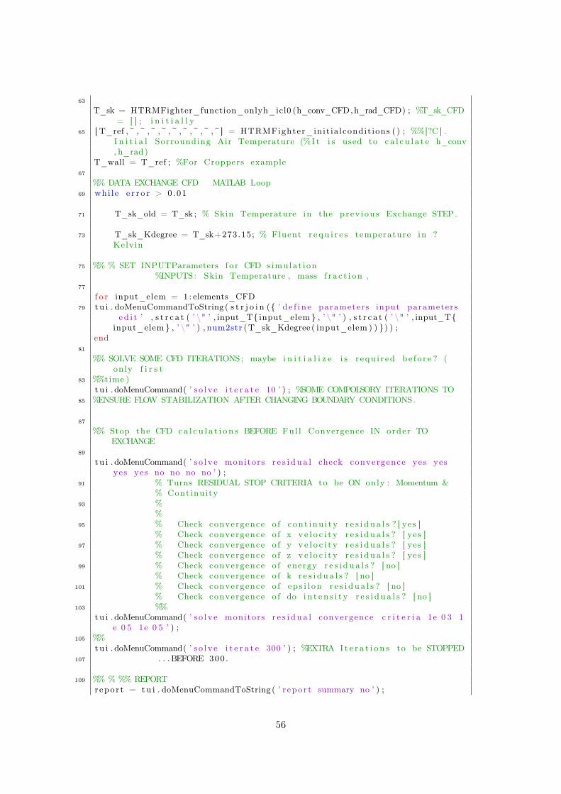
63
T_sk = HTRMFighter_function_onlyh_icl0 (h_conv_CFD,h_rad_CFD) ; %T_sk_CFD= [ ] ; i n i t i a l l y
65 [ T_ref ,~ ,~ ,~ ,~ ,~ ,~ ,~ ,~ ,~] = HTRMFighter_init ia lcondit ions ( ) ; %%[?C ] .I n i t i a l Sorrounding Air Temperature (%I t i s used to c a l c u l a t e h_conv, h_rad )
T_wall = T_ref ; %For Croppers example67
%% DATA EXCHANGE CFD MATLAB Loop69 whi le e r r o r > 0 .01
71 T_sk_old = T_sk ; % Skin Temperature in the prev ious Exchange STEP.
73 T_sk_Kdegree = T_sk+273.15; % Fluent r e qu i r e s temperature in ?Kelvin
75 %% % SET INPUTParameters f o r CFD s imu la t i on%INPUTS: Skin Temperature , mass f r a c t i on ,
77
f o r input_elem = 1 : elements_CFD79 t u i . doMenuCommandToString ( s t r j o i n ({ ’ d e f i n e parameters input parameters
ed i t ’ , s t r c a t ( ’ \" ’ , input_T{ input_elem } , ’ \" ’ ) , s t r c a t ( ’ \" ’ , input_T{input_elem } , ’ \" ’ ) , num2str (T_sk_Kdegree ( input_elem ) ) }) ) ;
end81
%% SOLVE SOME CFD ITERATIONS; maybe i n i t i a l i z e i s r equ i r ed be f o r e ? (only f i r s t
83 %%time )tu i . doMenuCommand( ’ s o l v e i t e r a t e 10 ’ ) ; %SOME COMPOLSORY ITERATIONS TO
85 %ENSURE FLOW STABILIZATION AFTER CHANGING BOUNDARY CONDITIONS.
87
%% Stop the CFD c a l c u l a t i o n s BEFORE Ful l Convergence IN order TOEXCHANGE
89
t u i . doMenuCommand( ’ s o l v e monitors r e s i d u a l check convergence yes yesyes yes no no no no ’ ) ;
91 % Turns RESIDUAL STOP CRITERIA to be ON only : Momentum &% Continuity
93 %%
95 % Check convergence o f c on t i nu i t y r e s i d u a l s ? [ yes ]% Check convergence o f x v e l o c i t y r e s i d u a l s ? [ yes ]
97 % Check convergence o f y v e l o c i t y r e s i d u a l s ? [ yes ]% Check convergence o f z v e l o c i t y r e s i d u a l s ? [ yes ]
99 % Check convergence o f energy r e s i d u a l s ? [ no ]% Check convergence o f k r e s i d u a l s ? [ no ]
101 % Check convergence o f e p s i l o n r e s i d u a l s ? [ no ]% Check convergence o f do i n t e n s i t y r e s i d u a l s ? [ no ]
103 %%tu i . doMenuCommand( ’ s o l v e monitors r e s i d u a l convergence c r i t e r i a 1e 0 3 1
e 0 5 1e 0 5 ’ ) ;105 %%
tu i . doMenuCommand( ’ s o l v e i t e r a t e 300 ’ ) ; %EXTRA I t e r a t i o n s to be STOPPED107 . . . BEFORE 300 .
109 %% % %% REPORTrepor t = tu i . doMenuCommandToString ( ’ r epo r t summary no ’ ) ;
56
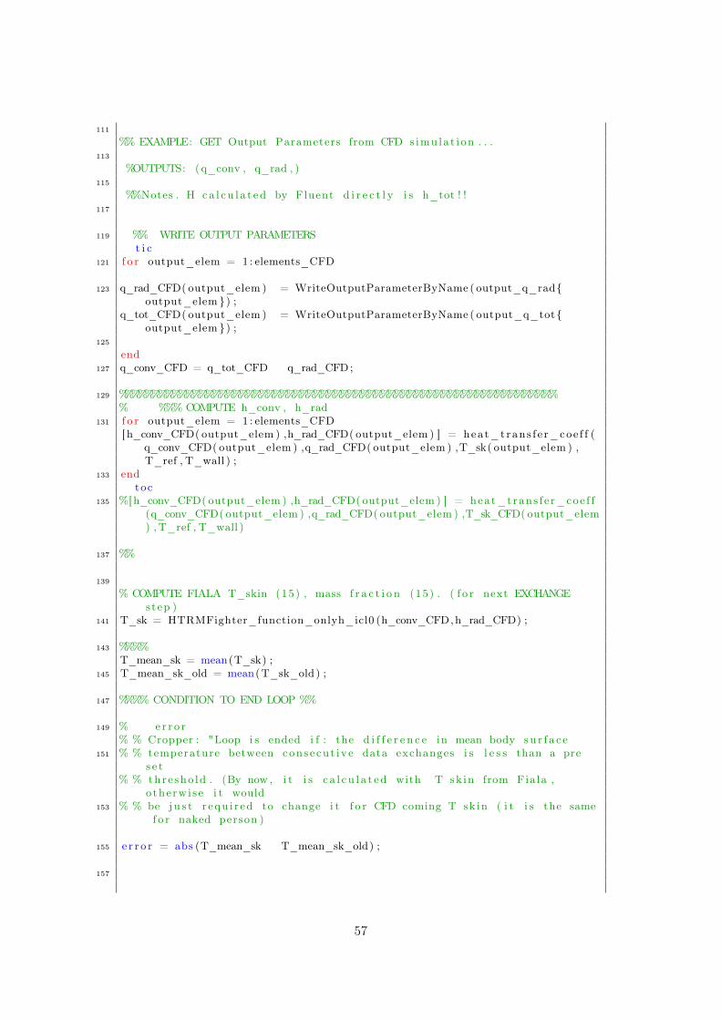
111
%% EXAMPLE: GET Output Parameters from CFD s imu la t i on . . .113
%OUTPUTS: (q_conv , q_rad , )115
%%Notes . H ca l c u l a t ed by Fluent d i r e c t l y i s h_tot ! !117
119 %% WRITE OUTPUT PARAMETERSt i c
121 f o r output_elem = 1 : elements_CFD
123 q_rad_CFD( output_elem ) = WriteOutputParameterByName ( output_q_rad{output_elem }) ;
q_tot_CFD( output_elem ) = WriteOutputParameterByName ( output_q_tot{output_elem }) ;
125
end127 q_conv_CFD = q_tot_CFD q_rad_CFD;
129 %%%%%%%%%%%%%%%%%%%%%%%%%%%%%%%%%%%%%%%%%%%%%%%%%%%%%%%%%%%%%%%%%% %%% COMPUTE h_conv , h_rad
131 f o r output_elem = 1 : elements_CFD[h_conv_CFD( output_elem ) ,h_rad_CFD( output_elem ) ] = heat_trans f e r_coe f f (
q_conv_CFD( output_elem ) ,q_rad_CFD( output_elem ) ,T_sk( output_elem ) ,T_ref , T_wall ) ;
133 endtoc
135 %[h_conv_CFD( output_elem ) ,h_rad_CFD( output_elem ) ] = heat_trans f e r_coe f f(q_conv_CFD( output_elem ) ,q_rad_CFD( output_elem ) ,T_sk_CFD( output_elem) ,T_ref , T_wall )
137 %%
139
% COMPUTE FIALA T_skin (15) , mass f r a c t i o n (15) . ( f o r next EXCHANGEstep )
141 T_sk = HTRMFighter_function_onlyh_icl0 (h_conv_CFD,h_rad_CFD) ;
143 %%%%T_mean_sk = mean(T_sk) ;
145 T_mean_sk_old = mean(T_sk_old ) ;
147 %%%% CONDITION TO END LOOP %%
149 % er r o r% % Cropper : "Loop i s ended i f : the d i f f e r e n c e in mean body su r f a c e
151 % % temperature between conse cu t i v e data exchanges i s l e s s than a pres e t
% % thre sho ld . (By now , i t i s c a l c u l a t ed with T sk in from Fiala ,o therwi se i t would
153 % % be j u s t r equ i r ed to change i t f o r CFD coming T sk in ( i t i s the samef o r naked person )
155 e r r o r = abs (T_mean_sk T_mean_sk_old) ;
157
57

159 % END OF THE EXCHANGE.% T_sk_near T_sk i s < x %. (That i s the d i f f e r e n c e between sk in o f CFD
and161 % sk in o f HTRM. ( with a WHILE in the BEGINNING)
%163 exchange = exchange+1;
f p r i n t f ( ’ Exchange Number has been completed %d , with an e r r o r %d ’ ,exchange , e r ror ’ ) ;
165 end
167 %%%% EXCHANGE FINISHED %%%%
169 di sp ( ’Data exchange has been completed Skin i s converged ’ ) ;
171 %% Run the CFD ca l c u l a t i o n s TO Ful l Convergence% After having sk in temperature s t a b i l i z e d , f low
nearby173 % might not have converged . Further CFD i t e r a t i o n s may
be% requ i r ed .
175
t u i . doMenuCommand( ’ s o l v e monitors r e s i d u a l check convergence yes yesyes yes yes yes yes ’ ) ; % Turns RESIDUAL STOP CRITERIA to be ON only :ALL.
177 t u i . doMenuCommand( ’ s o l v e monitors r e s i d u a l convergence c r i t e r i a 1e 0 5 1e 0 5 1e 0 5 1e 0 5 1e 0 5 1e 0 5 ’ ) ;
179 t u i . doMenuCommand( ’ s o l v e i t e r a t e 3000 ’ ) ; %EXTRA I t e r a t i o n s to beSTOPPED
. . .BEFORE 3000 .181
di sp ( ’CFD i s converged ’ ) ;
Listing 1: Code of coupling simulation - CFD-Matlab.
1 f unc t i on [ output_value ] = WriteOutputParameterByName ( output_parameter )
3
% This func t i on wr i t e s an Output parameter to Matlab that a l r eadye x i s t s in Fluent
5 %%
7 %% Inputs > Name o f the parameter ( in s t r i n g )
9 %% Outputs > Numerical va lue ( in long )
11 %% Modif ied l a s t time 27/04/2020 12 :35
13 %%%%%%%%%%%%%%%%%%%%%%%%%%%%%%%%%%%%%%%%%
15
orb=i n i t i a l i z e_o r b ( ) ; %i n i t i a l i z e aaS17 %load_ansys_aas ( ) ;
f l u e n t=a c t f l u e n t s e r v e r ( orb , ’ aaS_FluentId . txt ’ ) ; %connect to ANSYSproducts
19 t u i=f l u e n t . ge tSchemeContro l l e r Ins tance ( ) ;
21
58

one_param = tu i . doMenuCommandToString ( s t r j o i n ({ ’ d e f i n e parametersoutput parameters pr int to conso l e ’ , s t r c a t ( ’ \" ’ , output_parameter , ’\" ’ ) }) ) ; %obtains_1parameter
23 charonepam = char ( one_param) ; % Turns in to char the 1x1 automat i ca l l y saved s t r i n g in to > 1x460 p o s i t i o n s
pos_start = s t r f i n d ( charonepam , ’ . ’ ) 1 ; %To f i nd the p o s s i t i o no f the . which i n d i c a t e s the po s i t i o n o f the OUTPUT NUMERICAL VALUE
25 pos_end = s t r f i n d ( charonepam , ’ e+’ )+3; %To f i nd the p o s s i t i o no f the ’ e+’ which i n d i c a t e s the po s i t i o n o f the OUTPUT NUMERICALVALUE
27 output_value = str2num ( charonepam ( pos_start : pos_end ) ) ; %I t e x t r a c t s thevalue by cut p o s i t i o n s .
Listing 2: Write output parameter function from Fluent to Matlab.
59

Figure 27: Segmentation of body parts for the study developed in this report.
60