Changes to the Operational Forecasting System - ECMWF · The arti-cle on page 2 presents some of the rationale behind this c o u p l i n g . The economic aspect of weather forecasting

ECMWF Newsletter Number 80 – Summer 1998

In this issue

Editorial. . . . . . . . . . . . . . . . . . . . . . . . . . . . . . . . . 1

Changes to the Operational Forecast System . . . . 1

METEOROLOGICAL

Progress with wind-wave interaction. . . . . . . . . . . 2

Obtaining economic value from the EPS . . . . . . . . 8

Seasonal forecasting at ECMWF: an update . . . . 13

COMPUTING

Member State access to ECMWF’s computers -a progress report . . . . . . . . . . . . . . . . . . . . . . . . . 20

UNIX and Windows NT integration. . . . . . . . . . . 21

Computer User Documentation . . . . . . . . . . . . . . 22

GENERAL

ECMWF calendar. . . . . . . . . . . . . . . . . . . . . . . . . 22

ECMWF publications. . . . . . . . . . . . . . . . . . . . . . 22

Index of past newsletter articles . . . . . . . . . . . . . 23

Useful names and telephone numberswithin ECMWF . . . . . . . . . . . . . . . . . . . . . . . . . . 24

1

European Centre for Medium-RangeWeather Forecasts

Shinfield Park, Reading, RG2 9AX, UK

Fax: +44 118 986 9450

Telephone: National . . . . . . . . . . . . . 0118 949 9000

International . . . . . . . +44 118 949 9000

Internet URL . . . . . . . . . . . . . http://www.ecmwf.int

Cover

Wind and waves are now coupled in the latest cycleof the model - see page 2.

Editorial

Up to now ECMWF has run separate atmospheric andocean wave forecast models. With the introduction of thelatest cycle of the model, [namely Cycle 18 release 6 of theIntegrated Forecasting System (IFS)], ECMWF is running acoupled atmospheric ocean wave forecast model. The arti-cle on page 2 presents some of the rationale behind thisc o u p l i n g .

The economic aspect of weather forecasting is one of thecrucial considerations for end users of such forecasts. T h epotential economic benefits of the relatively new forecast-ing tool EPS (Ensemble Prediction System) comes underan initial scrutiny in the article on page 8.

An initial look at ECMWF’s work in the field of seasonalweather forecasting was given in ECMWF Newsletter No.77 (autumn 1997). A first update is now presented in thiscurrent issue (see pages 13-19), covering the recentdecline of the El Niño event.

Member State users can access ECMWF’s computer sys-tems via a variety of means, all of which are SecurID cardprotected. An update on these various card-protected ser-vices is given on page 20.

With Windows NT systems becoming more popular thequestion arises on integrating such systems into an exist-ing Unix based environment. There are various options,some of which are discussed in the article on page 21.

More and more of the computer documentation is becom-ing on-line based, especially around the concept of HTMLfiles. The article on page 22 outlines the Centre’s currentstatus in the move of its documentation to HTML.

Changes to theOperational Forecasting System

An hourly, two-way coupling of the atmospheric andocean-wave model was introduced on 29 June 1998.Predicted ocean waves now provide information to theatmospheric boundary layer.

Other modifications introduced at the same time(Cy18r6) were:1 . the use of both significant and standard level winds,

temperatures and humidities from radiosondes(geopotential is no longer used);

2 . the use of extra off-time data, mostly SYNOPs andD R I B U s ;

3 . the use of 1D-Var SSM/I total column water vapour;4 . extension of the use of GOES high-resolution winds

to the northern extratropics;5 . the use of more TOVS channels over land;6 . the observation operator for 10m winds is now unified

for scatterometer, DRIBU and SYNOP o b s e r v a t i o n s .


2

M E T E O RO L O G I CA L

Planned changes

u Increase in the number of model levels from 31 to 50,with the majority of the extra levels occurring in thestratosphere, the top of the model will be moved from10 to 0.1 hPa;

u Use of TOVS and ATOVS level Ib radiance data fromthe NOAA s a t e l l i t e s .

Brian Norris

In a previous Newsletter article (Janssen,1994) wediscussed some of the direct practical benefits of oceanwave forecasting and the benefits ocean wave informationmay have for atmospheric modelling and data assimila-tion. One of the benefits of ocean waves for the atmospheremay come from a more accurate treatment of the momen-tum exchange between atmosphere and the ocean surface,since the efficiency of the momentum exchange dependson the steepness of the ocean waves. Waves that are justgenerated by wind (we call this ‘young’ wind sea) aresteeper than mature wind seas. Steeper waves provide arougher surface and therefore give rise to a larger momen-tum transfer. We discussed a synoptic example whichshowed that the sea-state dependent momentum transfermay have consequences for the evolution of a depression,whilst there was also systematic impact on the climate ofthe atmosphere and the ocean waves. In the present articlewe shall describe some recent results we have obtainedwith Cy18R6 of the IFS which includes the effects of wind-wave interaction. In addition, since ocean waves are nowan integral part of the IFS, ensemble prediction of wavesis now part of the EPS. Afirst example is discussed, whichsuggests that the EPS for waves contains useful infor-mation on swell prediction in the medium range.

Model setup

Ocean waves affect the air-sea momentum transfer, andalso the heat and moisture transfer over the oceans. In theprevious versions of the atmospheric model the air- s e amomentum transfer was modelled by means of theCharnock relation for the roughness length. The Charnockrelation only models the average effect of ocean waves onthe momentum transfer and therefore this momentumtransfer depends only on wind speed. However, nowadaysit is known that the Charnock parameter used in theparametrization of the momentum transfer is not a constantbut may vary by a factor of 10 (typically from 0.01 to 0.1)depending on the stage of development of the ocean waves.In order to accommodate for this the theory of wind-waveinteraction was extended by including the feedback ofocean waves on the mean airflow, resulting in a sea-statedependent Charnock parameter (Komen et al,1994). Thisinteraction is currently known as two-way interaction andit requires the tight coupling of the atmospheric modeland the wave model. In this two-way interaction mode theatmospheric model determines the surface winds neededto generate the ocean waves, while the wave model deter-mines the amount of momentum that has been received

from the atmosphere, and uses that information to deter-mine the Charnock parameter which is returned to theatmospheric model. The effect is relevant in rapidly varyingcircumstances such as may occur near a low and nearfronts. Additional benefits of this tight coupling are thatthe wind fields that drive the waves may be updated morefrequently (previously this was done every 6 hours whilepresently winds are updated every hour) and that infor-mation such as the air-sea temperature difference and thea i r-sea density ratio may be passed to the wave model.

The atmospheric model has been modified to allow forthis two-way interaction. Also, the analysis suite waschanged. In 3D-Va r, the first guess is modified in a mannerconsistent with the coupled physics, while also A l t i m e t e rwave height data are assimilated. In 4D-Va r, both first-guess and trajectory calculations are performed in coupledmode, while the minimisation is done with a constantCharnock parameter. Altimeter data are assimilated inthe final trajectory.

R e s u l t s

Early results on weather forecasting with the presentsetup, but with earlier cycles of the IFS and T213 reso-lution, have been reported during the air-sea interactionsymposium last year (Janssen et al,1997). A l t h o u g hconsiderable synoptic differences were found in both fore-cast surface pressure and wave height field, in general thedifferences were found to be of small scale thereforeresulting in only a modest positive impact on scores foratmospheric parameters. However, impact on scores forwave height and surface wind speed was somewhat larger.

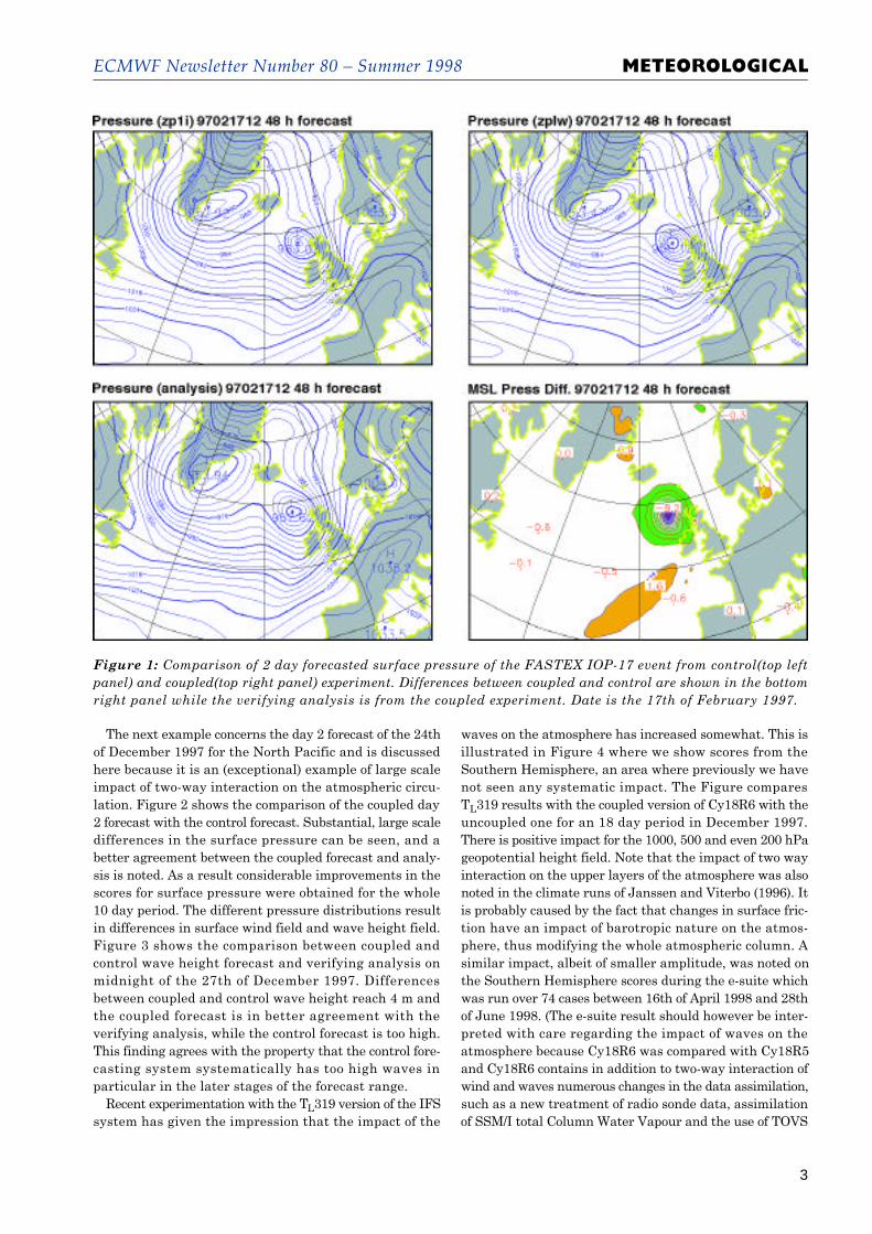
In order to illustrate the relatively small scale of theimpact of the sea state dependent roughness we discussthe case of a rapidly moving low from FASTEX. Thisevent started on the 17th of February just south of NewFoundland and arrived two days later west of Scotland.The day 2 forecast of this case is shown in Figure 1 andthe surface pressure in the run with two-way interac-tion (coupled for short) is lower by 7 hPa, in good agree-ment with the coupled analyzed pressure of that low.Such differences in surface pressure result in consider-able differences in the strength of the surface wind andtherefore in wave height. In this case the wave heightincreased from 9 to 13 m (not shown). Because of thesmall scale of the differences there is hardly any changein anomaly correlation over the North Atlantic area; infact, at day 2 of the forecast both coupled and controlexperiment have anomaly correlations close to 100%.

Progress with wind-wave interaction


3


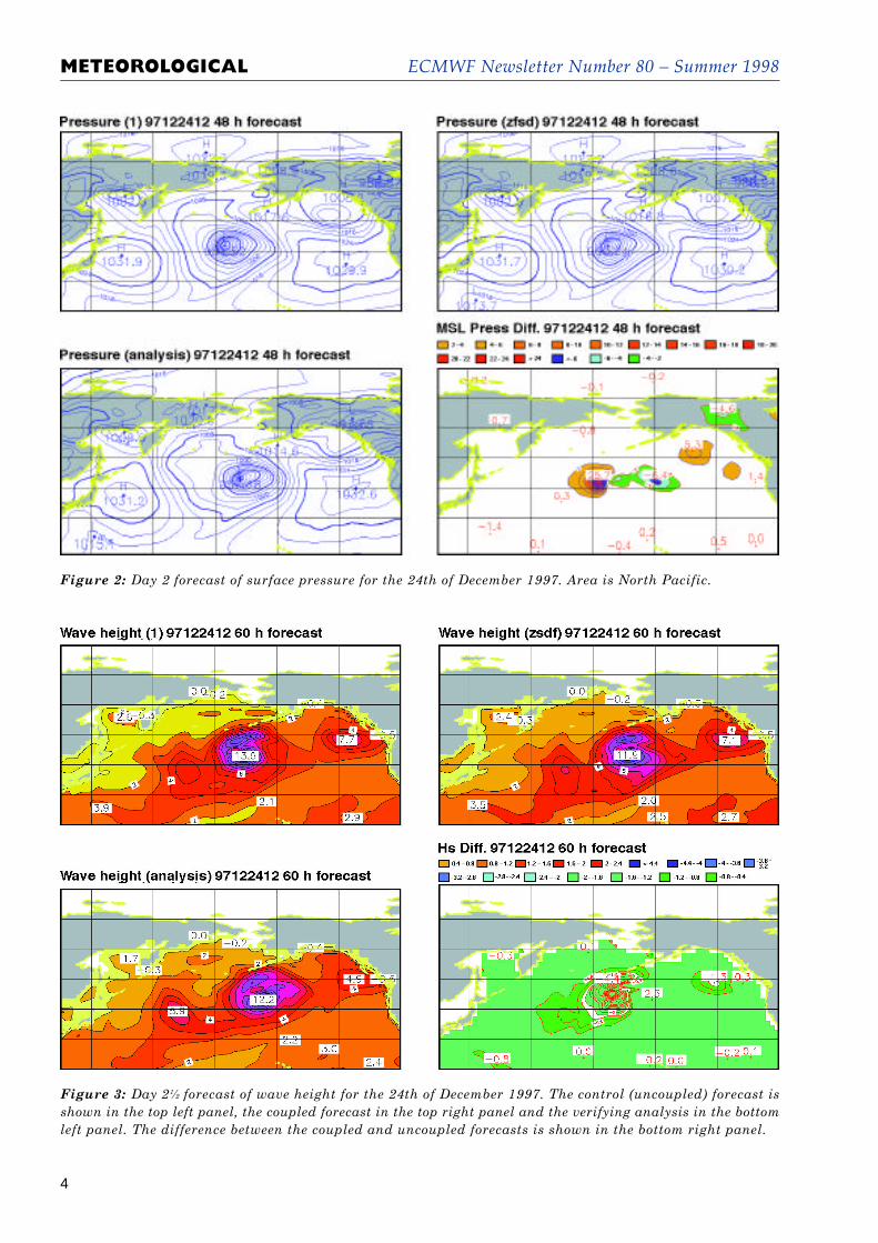
The next example concerns the day 2 forecast of the 24thof December 1997 for the North Pacific and is discussedhere because it is an (exceptional) example of large scaleimpact of two-way interaction on the atmospheric circu-lation. Figure 2 shows the comparison of the coupled day2 forecast with the control forecast. Substantial, large scaledifferences in the surface pressure can be seen, and abetter agreement between the coupled forecast and analy-sis is noted. As a result considerable improvements in thescores for surface pressure were obtained for the whole10 day period. The different pressure distributions resultin differences in surface wind field and wave height field.Figure 3 shows the comparison between coupled andcontrol wave height forecast and verifying analysis onmidnight of the 27th of December 1997. Differencesbetween coupled and control wave height reach 4 m andthe coupled forecast is in better agreement with theverifying analysis, while the control forecast is too high.This finding agrees with the property that the control fore-casting system systematically has too high waves inparticular in the later stages of the forecast range.

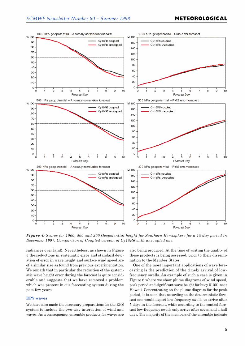
Recent experimentation with the TL319 version of the IFSsystem has given the impression that the impact of the

waves on the atmosphere has increased somewhat. This isillustrated in Figure 4 where we show scores from theSouthern Hemisphere, an area where previously we havenot seen any systematic impact. The Figure comparesTL319 results with the coupled version of Cy18R6 with theuncoupled one for an 18 day period in December 1997.There is positive impact for the 1000, 500 and even 200 hPageopotential height field. Note that the impact of two wayinteraction on the upper layers of the atmosphere was alsonoted in the climate runs of Janssen and Viterbo (1996). Itis probably caused by the fact that changes in surface fric-tion have an impact of barotropic nature on the atmos-phere, thus modifying the whole atmospheric column. Asimilar impact, albeit of smaller amplitude, was noted onthe Southern Hemisphere scores during the e-suite whichwas run over 74 cases between 16th of April 1998 and 28thof June 1998. (The e-suite result should however be inter-preted with care regarding the impact of waves on theatmosphere because Cy18R6 was compared with Cy18R5and Cy18R6 contains in addition to two-way interaction ofwind and waves numerous changes in the data assimilation,such as a new treatment of radio sonde data, assimilationof SSM/I total Column Water Vapour and the use of TOVS

Figure 1: Comparison of 2 day forecasted surface pressure of the FASTEX IOP-17 event from control(top leftpanel) and coupled(top right panel) experiment. Differences between coupled and control are shown in the bottomright panel while the verifying analysis is from the coupled experiment. Date is the 17th of February 1997.


4


Figure 2: Day 2 forecast of surface pressure for the 24th of December 1997. Area is North Pacific.

Figure 3: Day 2 1⁄2 forecast of wave height for the 24th of December 1997. The control (uncoupled) forecast isshown in the top left panel, the coupled forecast in the top right panel and the verifying analysis in the bottomleft panel. The difference between the coupled and uncoupled forecasts is shown in the bottom right panel.


5


Figure 4: Scores for 1000, 500 and 200 Geopotential height for Southern Hemisphere for a 18 day period inDecember 1997. Comparison of Coupled version of Cy18R6 with uncoupled one.

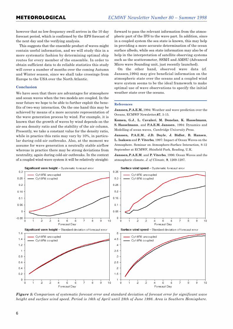
radiances over land). Nevertheless, as shown in Figure5 the reductions in systematic error and standard devi-ation of error in wave height and surface wind speed areof a similar size as found from previous experimentation.We remark that in particular the reduction of the system-atic wave height error during the forecast is quite consid-erable and suggests that we have removed a problemwhich was present in our forecasting system during thepast few years.

EPS waves

We have also made the necessary preparations for the EPSsystem to include the two-way interaction of wind andwaves. As a consequence, ensemble products for waves are

also being produced. At the time of writing the quality ofthese products is being assessed, prior to their dissemi-nation to the Member States.

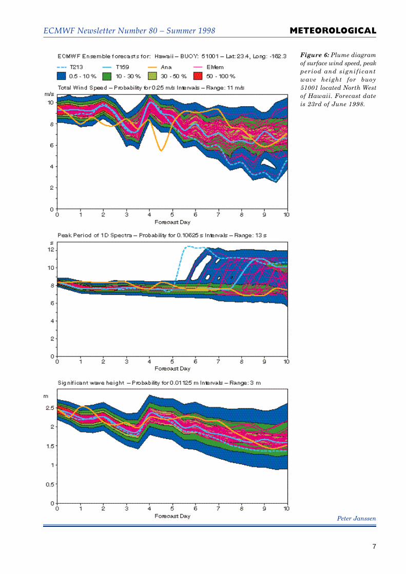
One of the most important applications of wave fore-casting is the prediction of the timely arrival of low-frequency swells. An example of such a case is given inFigure 6 where we show plume diagrams of wind speed,peak period and significant wave height for buoy 51001 nearHawaii. Concentrating on the plume diagram for the peakperiod, it is seen that according to the deterministic fore-cast one would expect low-frequency swells to arrive after5 days in the forecast, while according to the control fore-cast low-frequency swells only arrive after seven and a halfdays. The majority of the members of the ensemble indicate


6


however that no low-frequency swell arrives in the 10 dayforecast period, which is confirmed by the EPS forecast ofthe next day and the verifying analysis.

This suggests that the ensemble product of waves mightcontain useful information, and we will study this in amore systematic fashion by determining optimal shiproutes for every member of the ensemble. In order toobtain sufficient data to do reliable statistics this studywill cover a number of months over the coming A u t u m nand Winter season, since we shall take crossings fromEurope to the USA over the North A t l a n t i c .

C o n c l u s i o n

We have seen that there are advantages for atmosphereand ocean waves when the two models are coupled. In thenear future we hope to be able to further exploit the bene-fits of two-way interaction. On the one hand this may beachieved by means of a more accurate representation ofthe wave generation process by wind. For example, it isknown that the growth of waves by wind depends on thea i r-sea density ratio and the stability of the air column.P r e s e n t l y, we take a constant value for the density ratio,while in practice this ratio may vary by 10%, in particu-lar during cold-air outbreaks. Also, at the moment weassume for wave generation a neutrally stable airflowwhereas in practice there may be strong deviations fromn e u t r a l i t y, again during cold-air outbreaks. In the contextof a coupled wind-wave system it will be relatively straight-

forward to pass the relevant information from the atmos-pheric part of the IFS to the wave part. In addition, sincein a coupled system the sea state is known, this may helpin providing a more accurate determination of the oceansurface albedo, while sea state information may also be ofhelp in the interpretation of satellite observing systemssuch as the scatterometer, SSM/I and AMSU (AdvancedMicro wave Sounding unit, just recently launched).

On the other hand, observed wave data (cf.Janssen,1994) may give beneficial information on theatmospheric state over the oceans and a coupled windwave system seems to be the ideal framework to makeoptimal use of wave observations to specify the initialweather state over the oceans.

Figure 5: Comparison of systematic forecast error and standard deviation of forecast error for significant waveheight and surface wind speed. Period is 16th of April until 28th of June 1998. Area is Southern Hemisphere.

References

Janssen, P.A.E.M.,1994: Weather and wave prediction over the

Oceans, ECMWF Newsletter,67, 3-15.

Komen, G.J., L. Cavaleri, M. Donelan, K. Hasselmann,

S. Hasselmann , and P.A.E.M. Janssen , 1994: Dynamics and

Modelling of ocean waves, Cambridge University Press.

Janssen, P. A . E . M., J.D. Doyle , J. Bidlot , B. Hansen ,

L. Isaksen and P. Viterbo, 1997: Impact of Ocean Waves on the

Atmosphere. Seminar on Atmosphere-Surface Interaction, 8-12

September at ECMWF, Shinfield Park, Reading, U.K.

Janssen, P.A.E.M. and P. Viterbo, 1996: Ocean Waves and the

atmospheric climate. J. of Climate, 9, 1269-1287.


7


Peter Janssen

Figure 6: Plume diagramof surface wind speed, peakperiod and significantwave height for buoy51001 located North We s tof Hawaii. Forecast dateis 23rd of June 1998.


8


while L would be the economic loss due to traffic delaysand accidents on icy roads. The expense associated witheach combination of action and occurrence of E is shownin table 1 (the expense matrix).

The decision maker wishes to pursue a strategy whichwill minimise any losses over a large number of cases. Ifonly climatological information is available there arejust two options: either always take protective action ornever protect. Always taking action incurs a cost C on eachoccasion (irrespective of whether the event occurs or not),while if action is never taken the loss L occurs only on thatproportion o of occasions when the event occurs, hencethe average expense is oL. Thus in the absence of infor-mation other than climatology, the optimal course ofaction is always act if C < oL and never act otherwise.

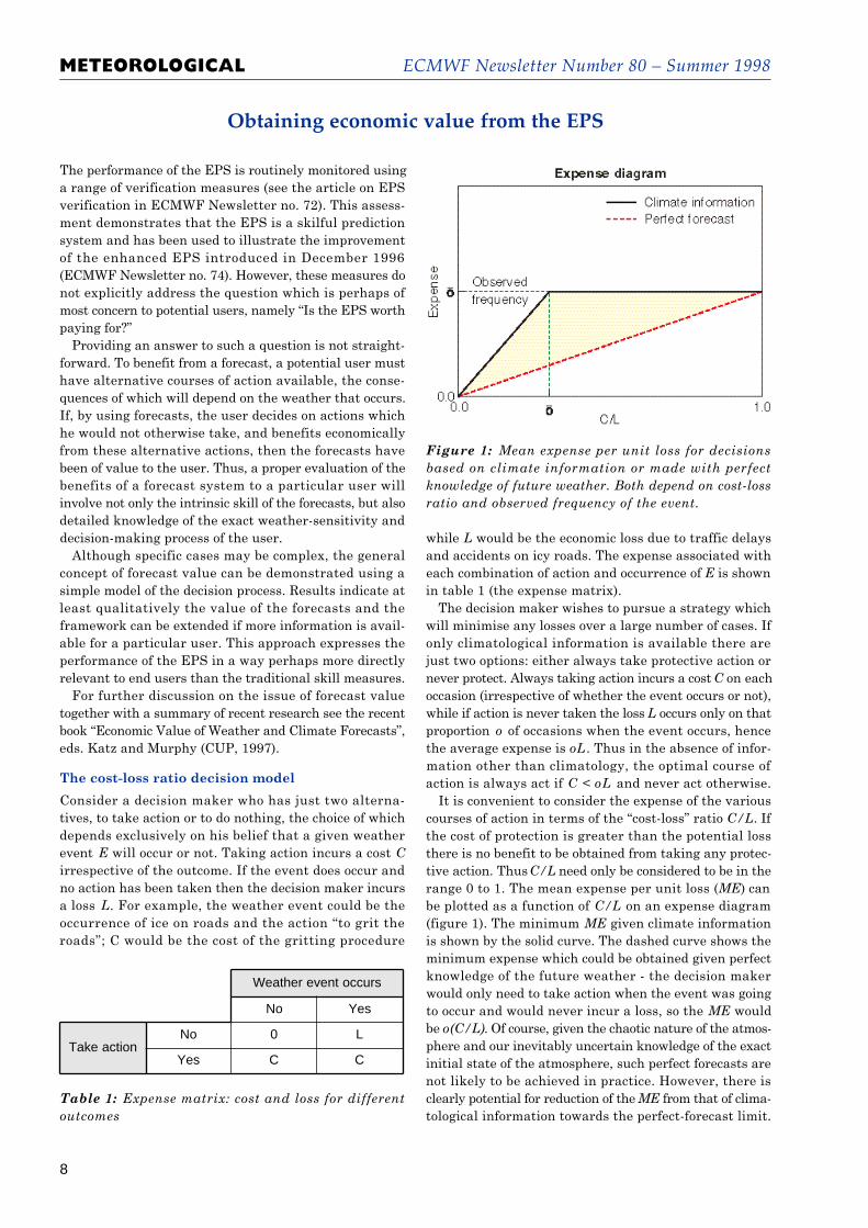
It is convenient to consider the expense of the variouscourses of action in terms of the “cost-loss” ratio C / L. Ifthe cost of protection is greater than the potential lossthere is no benefit to be obtained from taking any protec-tive action. Thus C / L need only be considered to be in therange 0 to 1. The mean expense per unit loss (M E) canbe plotted as a function of C / L on an expense diagram(figure 1). The minimum M E given climate informationis shown by the solid curve. The dashed curve shows theminimum expense which could be obtained given perfectknowledge of the future weather - the decision makerwould only need to take action when the event was goingto occur and would never incur a loss, so the M E w o u l dbe o( C / L ). Of course, given the chaotic nature of the atmos-phere and our inevitably uncertain knowledge of the exactinitial state of the atmosphere, such perfect forecasts arenot likely to be achieved in practice. However, there isclearly potential for reduction of the M E from that of clima-tological information towards the perfect-forecast limit.

The performance of the EPS is routinely monitored usinga range of verification measures (see the article on EPSverification in ECMWF Newsletter no. 72). This assess-ment demonstrates that the EPS is a skilful predictionsystem and has been used to illustrate the improvementof the enhanced EPS introduced in December 1996(ECMWF Newsletter no. 74). However, these measures donot explicitly address the question which is perhaps ofmost concern to potential users, namely “Is the EPS worthpaying for?”

Providing an answer to such a question is not straight-forward. To benefit from a forecast, a potential user musthave alternative courses of action available, the conse-quences of which will depend on the weather that occurs.If, by using forecasts, the user decides on actions whichhe would not otherwise take, and benefits economicallyfrom these alternative actions, then the forecasts havebeen of value to the user. Thus, a proper evaluation of thebenefits of a forecast system to a particular user willinvolve not only the intrinsic skill of the forecasts, but alsodetailed knowledge of the exact weather-sensitivity anddecision-making process of the user.

Although specific cases may be complex, the generalconcept of forecast value can be demonstrated using asimple model of the decision process. Results indicate atleast qualitatively the value of the forecasts and theframework can be extended if more information is avail-able for a particular user. This approach expresses theperformance of the EPS in a way perhaps more directlyrelevant to end users than the traditional skill measures.

For further discussion on the issue of forecast valuetogether with a summary of recent research see the recentbook “Economic Value of Weather and Climate Forecasts”,eds. Katz and Murphy (CUP, 1997).

The cost-loss ratio decision model

Consider a decision maker who has just two alterna-tives, to take action or to do nothing, the choice of whichdepends exclusively on his belief that a given weatherevent E will occur or not. Taking action incurs a cost Cirrespective of the outcome. If the event does occur andno action has been taken then the decision maker incursa loss L. For example, the weather event could be theoccurrence of ice on roads and the action “to grit theroads”; C would be the cost of the gritting procedure

Weather event occurs

No Yes

Take actionNo 0 L

Yes C C

Figure 1: Mean expense per unit loss for decisionsbased on climate information or made with perfectknowledge of future weather. Both depend on cost-lossratio and observed frequency of the event.

Table 1: Expense matrix: cost and loss for differento u t c o m e s

Obtaining economic value from the EPS


9


The provision of additional information in the form offorecasts may allow the decision maker to revise hisstrategy and reduce his expected expense. The extent bywhich the expense is reduced is a measure of the valueof the forecasts to the decision maker. We define the valueV of a forecast system as the reduction in ME as a propor-tion of that which would be achieved by a perfect forecast.Thus maximum value V = 1 will be obtained from a perfectforecast system, while V = 0 for a climate forecast. If V >0 then the user will benefit from the system.

Skill and value for a deterministic forecast system

Consider first a deterministic forecast system, that iseach forecast is a simple statement either that a givenweather event will occur or that it will not occur. The valueof the system depends on the hit rate (HR) and falsealarm rate (FAR) of the forecasts, on the observedfrequency of the event, and on the user-specific cost-lossratio (see appendix).

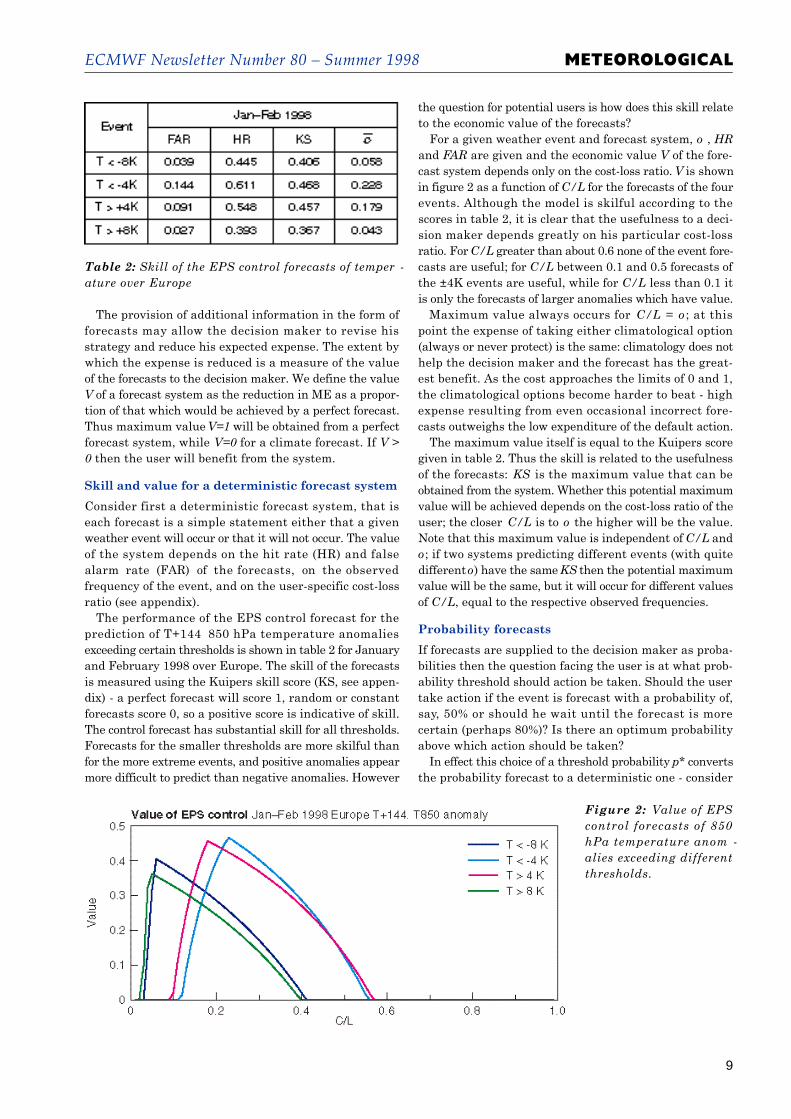
The performance of the EPS control forecast for theprediction of T+144 850 hPa temperature anomaliesexceeding certain thresholds is shown in table 2 for Januaryand February 1998 over Europe. The skill of the forecastsis measured using the Kuipers skill score (KS, see appen-d i x ) - a perfect forecast will score 1, random or constantforecasts score 0, so a positive score is indicative of skill.The control forecast has substantial skill for all thresholds.Forecasts for the smaller thresholds are more skilful thanfor the more extreme events, and positive anomalies appearmore difficult to predict than negative anomalies. However

the question for potential users is how does this skill relateto the economic value of the forecasts?

For a given weather event and forecast system, o , H Rand FA R are given and the economic value V of the fore-cast system depends only on the cost-loss ratio. V is shownin figure 2 as a function of C / L for the forecasts of the fourevents. Although the model is skilful according to thescores in table 2, it is clear that the usefulness to a deci-sion maker depends greatly on his particular cost-lossratio. For C / L greater than about 0.6 none of the event fore-casts are useful; for C / L between 0.1 and 0.5 forecasts ofthe ±4K events are useful, while for C / L less than 0.1 itis only the forecasts of larger anomalies which have value.

Maximum value always occurs for C / L = o ; at thispoint the expense of taking either climatological option(always or never protect) is the same: climatology does nothelp the decision maker and the forecast has the great-est benefit. As the cost approaches the limits of 0 and 1,the climatological options become harder to beat - highexpense resulting from even occasional incorrect fore-casts outweighs the low expenditure of the default action.

The maximum value itself is equal to the Kuipers scoregiven in table 2. Thus the skill is related to the usefulnessof the forecasts: K S is the maximum value that can beobtained from the system. Whether this potential maximumvalue will be achieved depends on the cost-loss ratio of theuser; the closer C / L is to o the higher will be the value.Note that this maximum value is independent of C / L a n do; if two systems predicting different events (with quitedifferent o) have the same K S then the potential maximumvalue will be the same, but it will occur for different valuesof C / L, equal to the respective observed frequencies.

Probability forecasts

If forecasts are supplied to the decision maker as proba-bilities then the question facing the user is at what prob-ability threshold should action be taken. Should the usertake action if the event is forecast with a probability of,s a y, 50% or should he wait until the forecast is morecertain (perhaps 80%)? Is there an optimum probabilityabove which action should be taken?

In effect this choice of a threshold probability p * c o n v e r t sthe probability forecast to a deterministic one - consider

Table 2: Skill of the EPS control forecasts of temper -ature over Europe

Figure 2: Value of EPScontrol forecasts of 850hPa temperature anom -alies exceeding differentt h r e s h o l d s .


10


those forecasts with higher probability for the event asforecasts that the event will occur and those with lowerprobability as forecasts the event will not occur. For agiven p *, the value of the system can then be determinedin the same way as for a deterministic system. By varyingp * from 0 to 1 a sequence of values for H R and FA R a n dhence V can be derived; the user can then choose thatvalue of p * which results in the largest value. Note thatsince V also depends on o and C / L the appropriate valueof p * will be different for different users and differentweather events.

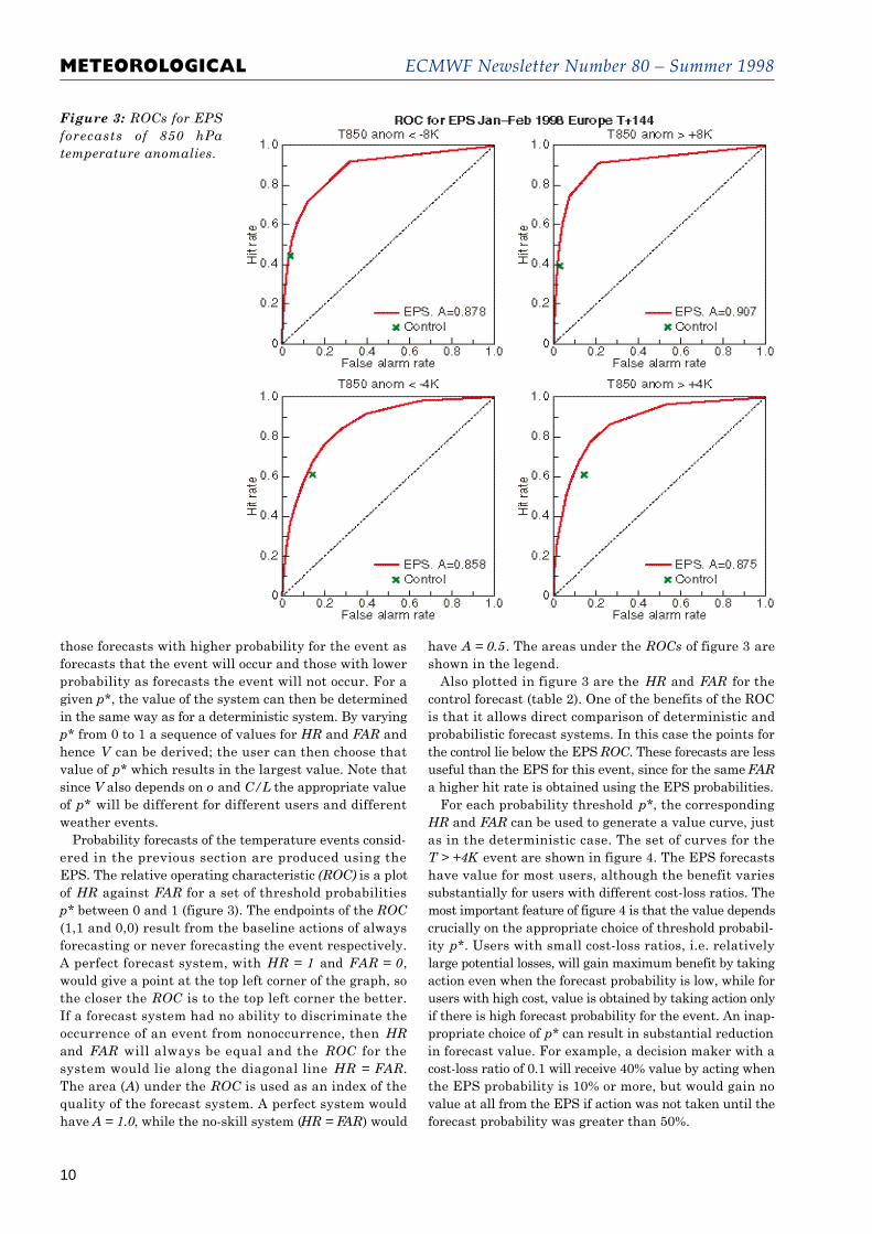
Probability forecasts of the temperature events consid-ered in the previous section are produced using theEPS. The relative operating characteristic ( R O C ) is a plotof H R against FA R for a set of threshold probabilitiesp * between 0 and 1 (figure 3). The endpoints of the R O C(1,1 and 0,0) result from the baseline actions of alwaysforecasting or never forecasting the event respectively.A perfect forecast system, with HR = 1 and FAR = 0,would give a point at the top left corner of the graph, sothe closer the R O C is to the top left corner the better.If a forecast system had no ability to discriminate theoccurrence of an event from nonoccurrence, then H Rand FA R will always be equal and the R O C for thesystem would lie along the diagonal line HR = FA R.The area (A) under the R O C is used as an index of thequality of the forecast system. A perfect system wouldhave A = 1.0, while the no-skill system (HR = FA R) would

have A = 0.5. The areas under the R O C s of figure 3 a r eshown in the legend.

Also plotted in figure 3 are the H R and FA R for thecontrol forecast (table 2). One of the benefits of the ROCis that it allows direct comparison of deterministic andprobabilistic forecast systems. In this case the points forthe control lie below the EPS R O C. These forecasts are lessuseful than the EPS for this event, since for the same FA Ra higher hit rate is obtained using the EPS probabilities.

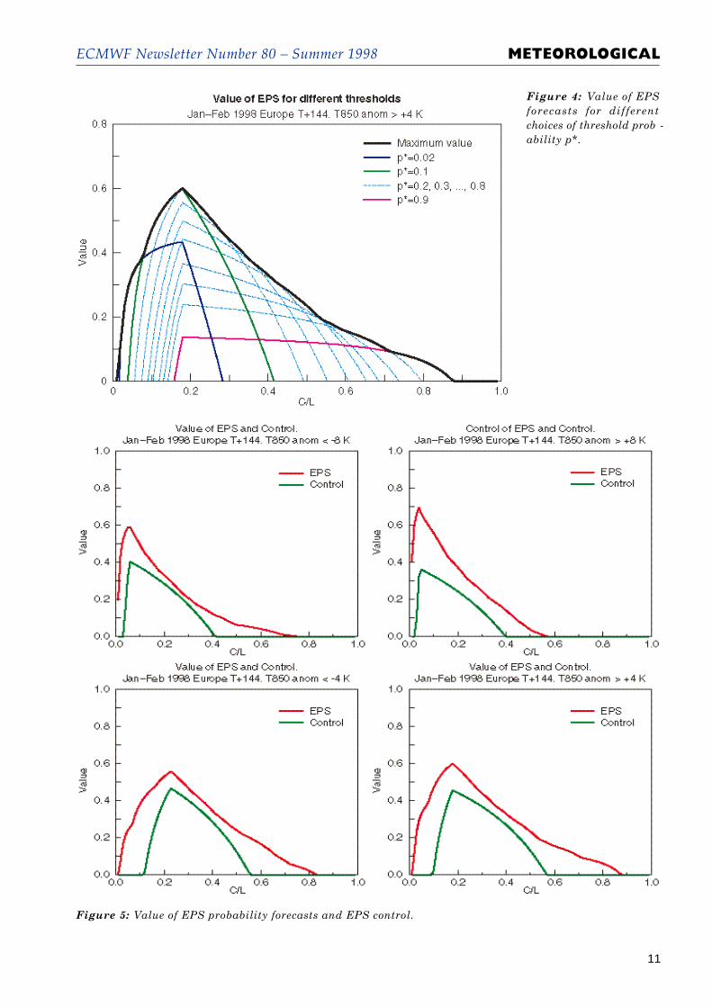
For each probability threshold p *, the correspondingH R and FA R can be used to generate a value curve, justas in the deterministic case. The set of curves for theT > +4K event are shown in figure 4. The EPS forecastshave value for most users, although the benefit variessubstantially for users with different cost-loss ratios. Themost important feature of figure 4 is that the value dependscrucially on the appropriate choice of threshold probabil-ity p *. Users with small cost-loss ratios, i.e. relativelylarge potential losses, will gain maximum benefit by takingaction even when the forecast probability is low, while forusers with high cost, value is obtained by taking action onlyif there is high forecast probability for the event. An inap-propriate choice of p * can result in substantial reductionin forecast value. For example, a decision maker with acost-loss ratio of 0.1 will receive 40% value by acting whenthe EPS probability is 10% or more, but would gain novalue at all from the EPS if action was not taken until theforecast probability was greater than 50%.

Figure 3: ROCs for EPSforecasts of 850 hPatemperature anomalies.


11


Figure 4: Value of EPSforecasts for differentchoices of threshold prob -ability p*.

Figure 5: Value of EPS probability forecasts and EPS control.


12


This example illustrates the important advantage ofproviding probability information to users: the value ofthe EPS forecasts depends significantly on the choice ofprobability threshold p * and on the user’s cost-loss ratio.There is no single threshold for which the EPS has valuefor all users - different users must use different thresh-olds to benefit from the forecasts. If the forecast is reducedto a single deterministic one for all users, for instance byusing the ensemble mean or by choosing an arbitrarythreshold, the value to some users will be reduced and mayeven be eliminated completely.

Comparison of the value curves for the EPS probabilityforecasts and the control deterministic forecast highlightsthe advantage of the probability forecasts (figure 5). Theflexibility of being able to choose the threshold probabil-ity greatly increases the range of users who will benefitfrom the forecasts. Even though the deterministic forecastsappear close to the EPS curves on the R O C s, the extravalue of the probability forecasts can be substantial.

C o n c l u s i o n s

There is no simple relationship between the skill of aforecasting system and the value of that system to users.A simple cost-loss model of economic value can be usedto give an indication of the potential benefit to a user ina more relevant way. While a system with no skill will nothave value, it is not necessarily the case that a skilfulsystem will be beneficial to a given user. The value of thesystem depends not only on the performance of the system(as measured by hit rate and false alarm rate) but alsoon the observed frequency of the event and, importantly,on the relevant costs of the user.

Probability forecasts are generally more useful thandeterministic forecasts of comparable quality because of thefacility for the user to select a probability threshold appro-priate to his needs. The arbitrary determination of such athreshold without knowledge of the particular user’srequirements can severely reduce the value of the system.

Although it may be difficult to determine the costs andlosses for a particular user (users themselves may notreadily have this information) the simple value curvespresented here do present the forecast verification in aform relevant to the user’s needs. The EPS will indeedhave economic value to many users, providing at day sixperhaps 60% of the savings which would be obtained withperfect knowledge of future weather. That surely is worthpaying for.

A p p e n d i x

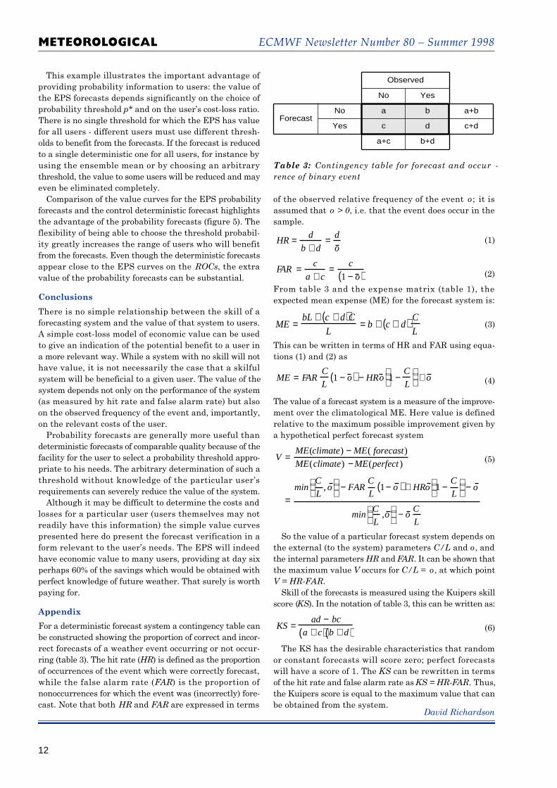
For a deterministic forecast system a contingency table canbe constructed showing the proportion of correct and incor-rect forecasts of a weather event occurring or not occur-ring (table 3). The hit rate (H R) is defined as the proportionof occurrences of the event which were correctly forecast,while the false alarm rate (FA R) is the proportion of nonoccurrences for which the event was (incorrectly) fore-cast. Note that both H R and FA R are expressed in terms

of the observed relative frequency of the event o; it isassumed that o > 0, i.e. that the event does occur in thes a m p l e .

Observed

No Yes

ForecastNo a b a+b

Yes c d c+d

a+c b+d

Table 3: Contingency table for forecast and occur -rence of binary event

So the value of a particular forecast system depends onthe external (to the system) parameters C / L and o, andthe internal parameters H R and FA R. It can be shown thatthe maximum value V occurs for C / L = o, at which pointV = HR-FA R .

Skill of the forecasts is measured using the Kuipers skillscore (K S). In the notation of table 3, this can be written as:

HR = d

b + d= d

o

FAR = c

a + c= c

1 − o( )

ME =bL + c + d( )C

L= b + c + d( ) C

L

ME = FARC

L1 − o( ) − HRo 1 −

C

L

+ o

V =ME(climate) − ME( forecast)

ME(climate) − ME(perfect )

=min

C

L, o

− FAR

C

L1− o( ) + HRo 1 −

C

L

− o

minC

L,o

− o

C

L

( 1 )

( 2 )

( 3 )

( 4 )

( 5 )

From table 3 and the expense matrix (table 1), theexpected mean expense (ME) for the forecast system is:

This can be written in terms of HR and FAR using equa-tions (1) and (2) as

The value of a forecast system is a measure of the improve-ment over the climatological ME. Here value is definedrelative to the maximum possible improvement given bya hypothetical perfect forecast system

KS =ad − bc

a + c( ) b + d( ) ( 6 )

The KS has the desirable characteristics that randomor constant forecasts will score zero; perfect forecastswill have a score of 1. The K S can be rewritten in termsof the hit rate and false alarm rate as KS = HR-FA R. Thus,the Kuipers score is equal to the maximum value that canbe obtained from the system.

David Richardson


13


The seasonal forecast system was described in the autumn1997 ECMWF newsletter (No 77). Since that time theECMWF Council gave approval for distribution of seasonalforecast products on the Wo r l d - Wi d e - Web in an experi-mental capacity. Forecasts within 35 degrees of the equatorare available to all on http://www.ecmwf.int. Member Statesmay access the full global products onhttp://w3ms/ecmwf/seasonal/index.html, but should beaware of the limitations of forecasts in the extratropics ingeneral and especially over Europe. As discussed in theautumn newsletter, any prediction must be probabilisticin nature. Our web pages give two maps for each predictedfield, the probability of occurrence and a measure of theamplitude. The fields currently posted are the integratedrainfall, the surface pressure and the 2 m temperature validat 00 UTC, together with plume diagrams of the SeaSurface Temperature (SST) in Niño3, (a key region in thecentral east equatorial Pacific). A full and thorough eval-uation of the skill of the seasonal prediction system has notbeen conducted so far. However, some preliminary remarksare appropriate. Results are shown here for both the recent97/98 El Niño and also for earlier years of this decade.

Seasonal forecasting does not allow exact predictions,even for seasonally averaged values, but it should bepossible to describe the probability distribution forw e a t h e r, and hence calculate probabilities for any spec-ified event. Our plots of the probability of above averagetemperature or rainfall are just one example of the sort

of product that can be made; other possibilities might bethe probability of mean temperature above a specificvalue or a quintile threshold, the probability of thenumber of rain days exceeding a certain value, the prob-ability of either the mean maximum or absolutemaximum temperature reaching a certain value, thenumber of heavy snowfall events, etc. The probabilisticnature of the forecasting makes verification a difficultissue, particularly because so far we have only a smallnumber of cases to study. For cases where the (forecast)probability distributions are not much shifted fromclimate, then it is hard to know whether the forecastwas good, unless perhaps the observed weather is veryextreme. An essentially null forecast such as this mightbe of use, of course, if one could be confident that itimplied that extreme weather would definitely not occur- but testing would have to cover many years to estab-lish this. On the other hand, if the forecast is for a strongshift in the weather patterns for a particular year, thenthis provides a good opportunity to test the forecastsystem. It is still true that we are not able to predictexactly what will happen, but the test as to whether theobservations lie within the predicted range becomes morepowerful. In 1997 and 1998 our system has been fore-casting strong shifts in global weather patterns, largelyassociated with the exceptional El Niño. This means thatthe last year or so are a very good period over which toassess the performance of our system. Afuller assessment

Seasonal forecasting at ECMWF: an update

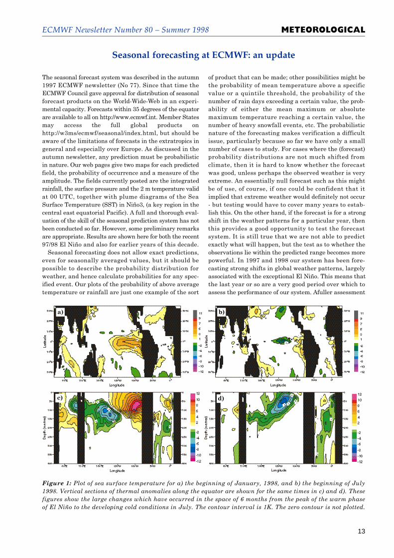
Figure 1: Plot of sea surface temperature for a) the beginning of January, 1998, and b) the beginning of July1998. Vertical sections of thermal anomalies along the equator are shown for the same times in c) and d). Thesefigures show the large changes which have occurred in the space of 6 months from the peak of the warm phaseof El Niño to the developing cold conditions in July. The contour interval is 1K. The zero contour is not plotted.

a ) b )

c ) d )


14


will require the completion and analysis of forecastscovering a much longer period of time; this will beprovided at some stage in the future.

The largest signal in the climate system on interannualtimescales is that of El Niño. Last year saw one of thebiggest recorded, in some respects bigger than 1982/3. May1998 saw a precipitous decline in temperatures in thecentral equatorial Pacific which by early June had ceasedto be warm and are now below average. There is thedistinct possibility of a cold phase developing, sometimesknown as La Niña. Figure 1a) shows the sea surfacetemperature anomalies at the beginning of January of thisy e a r, while Figure 1b) shows them at the beginning of Julyillustrating the rapid decay from warm anomalies of 5Kto cold anomalies of -2K. Figures 1c) and 1d) show thetemperature anomalies in the upper 400 m along theequator for the same times. The black vertical bandsindicate the equatorial land masses which separate the

three ocean basins. The temperatures in the subsurfaceocean have changed by an even greater amount than atthe surface, from a warm anomaly of 11K to a coldanomaly of -6K. In January ’98, even though the surfaceand subsurface temperatures were very strongly aboveaverage in the east, the subsurface temperatures were coldin the west. This cold anomaly spread slowly eastwardover the following 6 months to reach the surface in June.

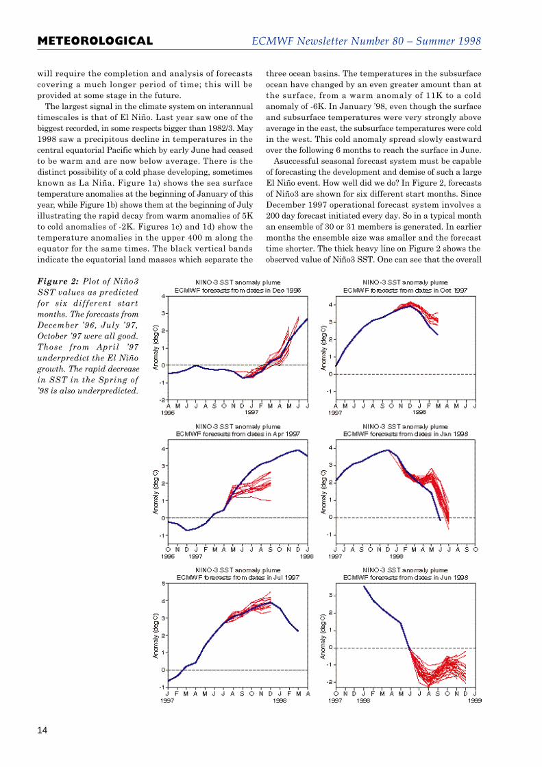
Asuccessful seasonal forecast system must be capableof forecasting the development and demise of such a largeEl Niño event. How well did we do? In Figure 2, forecastsof Niño3 are shown for six different start months. SinceDecember 1997 operational forecast system involves a200 day forecast initiated every day. So in a typical monthan ensemble of 30 or 31 members is generated. In earliermonths the ensemble size was smaller and the forecasttime shorter. The thick heavy line on Figure 2 shows theobserved value of Niño3 SST. One can see that the overall

Figure 2: Plot of Niño3SST values as predictedfor six different startmonths. The forecasts fromDecember ’96, July ’97,October ’97 were all good.Those from April ’97underpredict the El Niñogrowth. The rapid decreasein SST in the Spring of’98 is also underpredicted.


15


ability of our system to forecast Niño3 SST’s in 1997/98has been good, better indeed than might have beene x p e c t e d .

There have been times, however, when the forecastshave been less good. Some of our worst forecasts of Niño3S S Ts were those initiated in April ’97. All members of theensemble in this case underpredicted the growth of theanomaly as Figure 2b) shows. In March ’97, a majorIntraseasonal Oscillation with associated We s t e r l y - Wi n d -Bursts came out of the Indian Ocean into the west Pacificwhere large amplitude oceanic Kelvin-type waves weregenerated. These waves were strongly present in the oceanmodel initial conditions for forecasts initiated in April: itis surprising then that the model underpredicted theNiño3 SST. The reasons for this are not clear but there issome suggestion that the coupled model failed to amplifythe signal when it reached the east Pacific. The otherpanels of Figure 2 show that forecasts from December 96,and July ’97 were accurate, while those from October ’97slightly over-predicted the anomaly. Those initiated fromJanuary ’98 show a very tight ensemble and indicated avery rapid decay of the El Niño. In fact Nature showed an

even faster decline. The final panel predicts that coldconditions will last throughout the rest of the year.

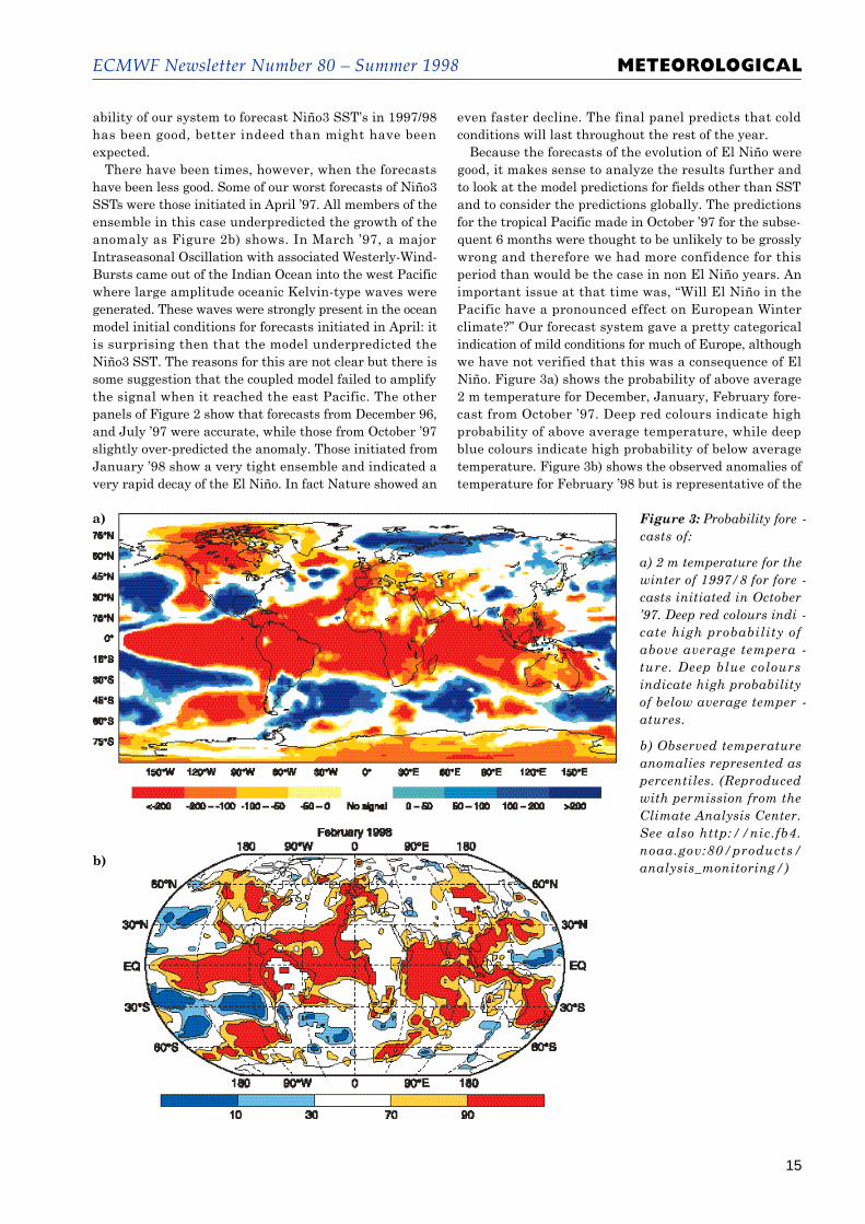
Because the forecasts of the evolution of El Niño weregood, it makes sense to analyze the results further andto look at the model predictions for fields other than SSTand to consider the predictions globally. The predictionsfor the tropical Pacific made in October ’97 for the subse-quent 6 months were thought to be unlikely to be grosslywrong and therefore we had more confidence for thisperiod than would be the case in non El Niño years. A nimportant issue at that time was, “Will El Niño in thePacific have a pronounced effect on European Wi n t e rclimate?” Our forecast system gave a pretty categoricalindication of mild conditions for much of Europe, althoughwe have not verified that this was a consequence of ElNiño. Figure 3a) shows the probability of above average2 m temperature for December, January, February fore-cast from October ’97. Deep red colours indicate highprobability of above average temperature, while deepblue colours indicate high probability of below averagetemperature. Figure 3b) shows the observed anomalies oftemperature for February ’98 but is representative of the

Figure 3: Probability fore -casts of:

a) 2 m temperature for thewinter of 1997/8 for fore -casts initiated in October’97. Deep red colours indi -cate high probability ofabove average tempera -ture. Deep blue coloursindicate high probabilityof below average temper -a t u r e s .

b) Observed temperatureanomalies represented aspercentiles. (Reproducedwith permission from theClimate Analysis Center.See also http://nic.fb4.n o a a . g o v : 8 0 / p r o d u c t s /a n a l y s i s _ m o n i t o r i n g / )

a )

b )


16


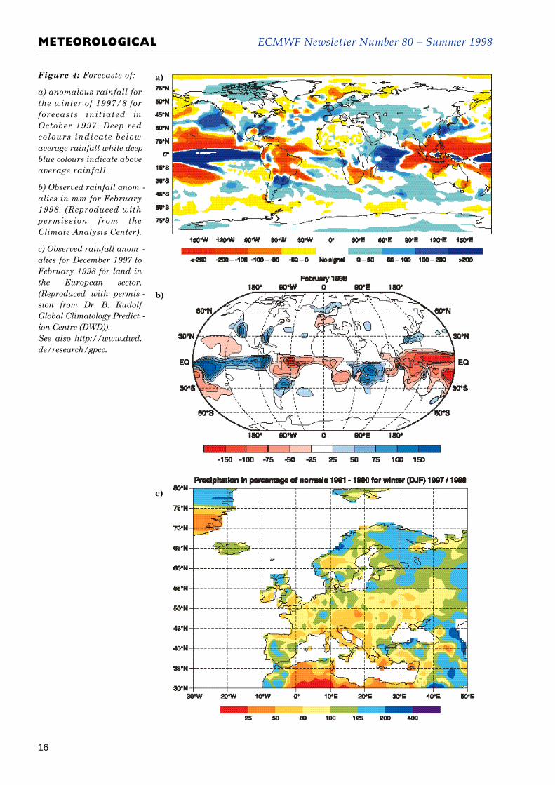
Figure 4: Forecasts of:

a) anomalous rainfall forthe winter of 1997/8 forforecasts initiated inOctober 1997. Deep redcolours indicate belowaverage rainfall while deepblue colours indicate aboveaverage rainfall.

b) Observed rainfall anom -alies in mm for February1998. (Reproduced withpermission from theClimate Analysis Center).

c) Observed rainfall anom -alies for December 1997 toFebruary 1998 for land inthe European sector.(Reproduced with permis -sion from Dr. B. RudolfGlobal Climatology Predict -ion Centre (DWD)).See also http://www.d w d .d e / r e s e a r c h / g p c c .

a )

b )

c )


17


earlier winter months. It does not correspond exactly tothe forecast product, showing percentile behaviour, butindicates the very unusual warm conditions of the winterof 97/98. The similarity of this map and the probabilitymap shown in Figure 3a) and in particular by the warmtropical Atlantic and the broad sweep of warmth from thesouthern Caribbean east/northeast to Europe is striking.North America was also warm in both predictions andobservations. There are apparent disagreements in theSouthern United States where below average tempera-tures were forecast in Figure 3a), but none observed onFigure 3b). In fact this region was cooler than normalthough not as cool as forecast. There is no warm anomalyover Brazil in the analysis, but this just indicates lack ofdata rather than the absence of an anomaly.

Figure 4a) shows the probability for rainfall anomalies.Rainfall is a more chaotic variable, less likely to be skilfuland more difficult to verify because of its small scalechaotic variability, but we include it here because of itspotential importance. Figure 4b) is one estimate of rain-fall for one month covering both land and sea. A l t h o u g hFigure 4b) is global and useful to give an estimate oftropical anomalies it is not useful for validating the predic-tions for the extra-tropics. A more detailed map fromGPCC (Global Precipitation Climatology Centre) cover-ing the same 3-month period as the forecasts, but justavailable for European land areas, is given in Figure 4c).Figure 4a) shows a general tendency for wetter northernEurope and, if anything, drier southern Europe, with theexception of Portugal and western Spain in the forecasts,while the verifications of Figure 4c) show similar patternsthough they differ in detail. Indeed this figure showsclearly the small-scale structure of the observed rainfallanomalies. Such detail can not be reproduced by the

coupled model whose resolution is much coarser thanthat observed. Detailed verification on a country bycountry basis is unlikely to be meaningful. In the tropicsthe broad-scale patterns of drought over the Indonesianregion and over Amazonia seen in Figure 4b) are well fore-cast, though here too they differ in detail.

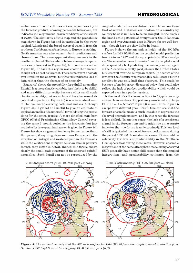
Figure 5 shows the anomalous height of the 500 hPasurface for DJF 97/98 from the coupled model predictionfrom October 1997 and the appropriate ECMWF analy-sis. The ensemble mean forecasts from the coupled modeldid a splendid job of predicting the anomaly in the regionof the Aleutians, a pretty good job over the United Statesbut less well over the European region. The centre of thelow over the Atlantic was reasonably well located but itsamplitude was only half that observed. This could bebecause of model error, discussed below, but could alsoreflect the lack of perfect predictability which would beexpected even in a perfect system.

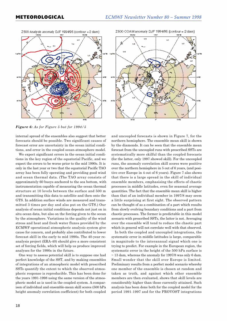
Is the level of skill shown on figs 2 to 5 typical or onlyattainable in windows of opportunity associated with largeEl Niño or La Nina’s? Figure 6 is similar to Figure 5except for a different year 1994/5. One can see that theforecast ensemble mean is much less able to represent theobserved anomaly pattern, and in this sense the forecastis less skilful. (In another sense, the lack of a consistentsignal in the forecast ensemble might be an accurateindicator that the future is undetermined). This low levelof skill is typical of the model forecast performance duringthe period 1991-96. A substantial cause of this could berelatively low levels of predictability in the NorthernHemisphere flow during these years. However, ensembleintegrations of the same atmosphere model using observedS S Ts generally have better skill scores than the coupledintegrations, and predictability estimates from the

Figure 5: The anomalous height of the 500 hPa surface for DJF 97/98 from the coupled model prediction fromOctober 1997 (right) and the verifying ECMWF analysis (left).


18


internal spread of the ensembles also suggest that betterforecasts should be possible. Two significant causes offorecast error are uncertainty in the ocean initial condi-tions, and error in the coupled ocean-atmosphere model.

We expect significant errors in the ocean initial condi-tions in the key region of the equatorial Pacific, and weexpect the errors to be worse prior to the mid 1990s. It isonly in the last year or two that the equatorial Pacific TA Oarray has been fully operating and providing good windand ocean thermal data. (The TAO array consists ofapproximately 60 buoys anchored to the sea bottom, withinstrumentation capable of measuring the ocean thermalstructure at 10 levels between the surface and 500 mand transmitting this data to satellite and then onto theGTS. In addition surface winds are measured and trans-mitted 3 times per day and also put on the GTS.) Ouranalysis of ocean initial conditions depends not just on insitu ocean data, but also on the forcing given to the oceanby the atmosphere. Variations in the quality of the windstress and heat and fresh water fluxes provided by theECMWF operational atmospheric analysis system givecause for concern, and probably also contributed to lowerforecast skill in the early to mid 1990s. The 40-year re-analysis project (ERA-40) should give a more consistentset of forcing fields, which will help us produce improvedanalyses for the 1990s in the future.

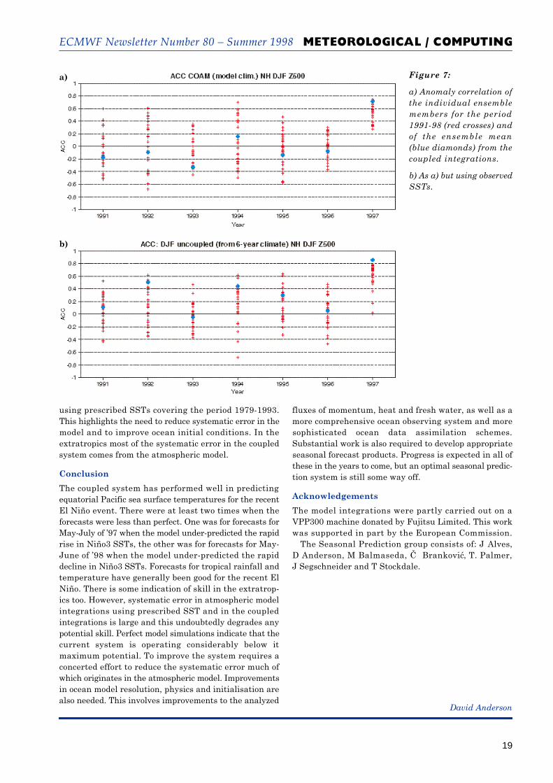
One way to assess potential skill is to suppose one hadperfect knowledge of the SST, and by making ensemblesof integrations of an atmospheric model with prescribedS S Ts quantify the extent to which the observed atmos-pheric response is reproducible. This has been done forthe years 1991-1998 using the same version of the atmos-pheric model as is used in the coupled system. A c o m p a r-ison of individual and ensemble-mean skill scores (500 hPaheight anomaly correlation coefficient) for both coupled

and uncoupled forecasts is shown in Figure 7, for thenorthern hemisphere. The ensemble mean skill is shownby the diamonds. It can be seen that the ensemble meanforecast from the uncoupled runs with prescribed SSTs aresystematically more skilful than the coupled forecasts(for the latter, only 1997 showed skill). For the uncoupledruns, the anomaly correlation skill scores were positiveover the northern hemisphere in 5 out of 6 years, (and posi-tive over Europe in 4 out of 6 years). Figure 7 also showsthat there is a large spread in the skill of individualensemble members, emphasising the effects of chaoticprocesses in middle latitudes, even for seasonal averagequantities. The fact that the ensemble mean skill is higherthan that of an individual member in 1997/8 may seema little surprising at first sight. The observed patterncan be thought of as a combination of a part which resultsfrom slowly evolving boundary conditions and a part fromchaotic processes. The former is predictable in this modelscenario with prescribed SSTs, the latter is not. Av e r a g i n gover the ensemble will tend to reduce the chaotic partwhich in general will not correlate well with that observed.

In both the coupled and uncoupled integrations, thesystematic error in middle latitudes is large, comparablein magnitude to the interannual signal which one istrying to predict. For example in the European region, thesystematic error in the height of the 500 hPa surface is~ 13 dam, whereas the anomaly for 1997/8 was only 6 dam.Small wonder that the skill over Europe is limited.Preliminary results from a perfect model scenario wherebyone member of the ensemble is chosen at random andtaken as truth, and against which other ensemblemembers are then evaluated, shows that skill levels areconsiderably higher than those currently attained. Suchanalysis has been done both for the coupled model for theperiod 1991-1997 and for the PROVOST integrations

Figure 6: As for Figure 5 but for 1994/5


19

M E T E O RO L O G I CAL / COMPUTING

using prescribed SSTs covering the period 1979-1993.This highlights the need to reduce systematic error in themodel and to improve ocean initial conditions. In theextratropics most of the systematic error in the coupledsystem comes from the atmospheric model.

C o n c l u s i o n

The coupled system has performed well in predictingequatorial Pacific sea surface temperatures for the recentEl Niño event. There were at least two times when theforecasts were less than perfect. One was for forecasts forMay-July of ’97 when the model under-predicted the rapidrise in Niño3 SSTs, the other was for forecasts for May-June of ’98 when the model under-predicted the rapiddecline in Niño3 SSTs. Forecasts for tropical rainfall andtemperature have generally been good for the recent ElNiño. There is some indication of skill in the extratrop-ics too. However, systematic error in atmospheric modelintegrations using prescribed SST and in the coupledintegrations is large and this undoubtedly degrades anypotential skill. Perfect model simulations indicate that thecurrent system is operating considerably below itmaximum potential. To improve the system requires aconcerted effort to reduce the systematic error much ofwhich originates in the atmospheric model. Improvementsin ocean model resolution, physics and initialisation arealso needed. This involves improvements to the analyzed

fluxes of momentum, heat and fresh water, as well as amore comprehensive ocean observing system and moresophisticated ocean data assimilation schemes.Substantial work is also required to develop appropriateseasonal forecast products. Progress is expected in all ofthese in the years to come, but an optimal seasonal predic-tion system is still some way off.

A c k n o w l e d g e m e n t s

The model integrations were partly carried out on aVPP300 machine donated by Fujitsu Limited. This workwas supported in part by the European Commission.

The Seasonal Prediction group consists of: J A l v e s ,D Anderson, M Balmaseda, C B r a n k o v ic, T. Palmer,J Segschneider and T Stockdale.

Figure 7:

a) Anomaly correlation ofthe individual ensemblemembers for the period1991-98 (red crosses) andof the ensemble mean(blue diamonds) from thecoupled integrations.

b) As a) but using observedS S Ts .

a )

b )

David Anderson


20

C O M P U T I N G

Three previous Newsletter articles have discussed whyan access system based on smart cards was consid-ered necessary (Newsletter No. 67, pp. 27-33), andthen its implementation (Newsletters No. 70, pp. 18/19& No. 73, pp. 30/31). This article reports on furtherp r o g r e s s .

During the course of 1994 the Centre successfullyconducted a “secure batch trial” to evaluate whether itwould be possible to adapt a smart card system toauthenticate users in a batch job environment. A f t e rapproval by the Technical Advisory Committee a proposalfor a smart card authentication system was acceptedby the Council at the end of 1994 and SecurID smartcards from Security Dynamics were chosen as the methodof control.

In 1995 and 1996 various SecurID-card-protectedservices were introduced and have subsequently beenenhanced and extended. Some of these services requirespecial ECMWF software: the ecbatch software packageis available to all Member States for all major UNIXp l a t f o r m s .

SecurID cards

Early this year the majority of SecurID cards wererenewed, as the first set of cards distributed to the MemberStates was about to expire. This operation went verysmoothly and the Member State Computing Repre-sentatives who are responsible for the local administra-tion had only a little extra work to do.

Te l n e t

The only UNIX server directly reachable from MemberStates via telnet is ‘[email protected]’. Telnet to ‘ecgate1’is also possible via the Centre’s firewall from specificInternet sites. All external access to ‘ecgate1’ and thefirewall is authenticated via SecurID smart cards. From‘ e c g a t e 1 ’ batch jobs can be submitted and a remote shell(rsh) invoked to ‘ecgate2’ and to the Centre’s Fujitsusystems without further validation.

Ecbatch/eccmd utility (ecqsub, ecqstat, ecqdel)

The ecbatch/eccmd utility allows Member State users tosubmit batch jobs from their local systems to ECMWF (the‘ e c q s u b ’ function), plus carry out some job managementfunctions (job status, job deletion, etc.).

Requests are authenticated with certificate-based signa-tures. To generate a certificate, the user will be promptedfor his/her ECMWF user identifier and SecurID PA S S-CODE. The certificate is valid for ecqsub requests for aperiod of 12 hours from the time of its generation (7 daysfor ecqdel and ecqstat).

Originally it was necessary for the user to be logged inon a Member State system which has TCP/IP access [email protected] via the leased lines. This restriction

has been removed and access is now possible via theInternet both from Member State systems and specificnon-Member State sites.

File transfer (ftp, eccopy, ecput, ecget, ecls)

Incoming ftp requests require strong authentication. [email protected] now offers a version of ftp whichprompts for smart card authentication rather than pass-words. Files destined for another ECMWF host have tobe transferred to [email protected] first, and then copiedto the other host or accessed via NFS.

Eccopy provides a means to send files to a remote sitefrom ECMWF without the need for ftp. It was originallyonly available via the leased lines to Member States.This restriction has also been removed and transfers arenow possible via the Internet to Member State systemsand specific non-Member State sites.

Ecput, ecget and ecls are further functions of theecbatch/eccmd utility. They provide file transfer to andfrom ECMWF, plus file display.

M A R S

MARS client software requires ecbatch/eccmd software tobe installed because it uses one of the ecbatch/eccmdfunctions to validate MARS retrievals. The MARS clientallows users to submit retrieval requests direct to theMARS system at ECMWF, without the need for batchjobs or interactive sessions at ECMWF.

The Member State user generates a MARS requestl o c a l l y. The MARS client will then obtain a signaturefrom the ecbatch/eccmd software, connect to the MARSserver running on an ECMWF host and transmit thesigned request. Certificates for signing MARS requestsexpire after three months, which makes such MARSrequests suitable for automated processing withinMember States.

The validation of MARS requests from CooperatingMember States happens in the same fashion as for fullMember States, but all other ECBATCH functions ared i s a b l e d .

Future plans

The Centre is planning to extend the file functions of theecbatch/eccmd utility to interface with ECFS permittingdirect file exchange between Member States and theC e n t r e ’s Data Handling System.

Dieter Niebel

Member State access to ECMWF’s computers - a progress report


21

C O M P U T I N G

In any computing environment there will be a mixtureof systems and in several installations today, includingthe European Centre for Medium-Range We a t h e rForecasts, this mixture includes UNIX and NT basedsystems. In order to make best use of these systems theyneed to be able to interoperate. This can be achieved viaseveral different degrees of integration.

Microsoft has become a major force in the world ofcomputing and has effectively defined de facto standardsfor office automation with packages like Wo r d ,PowerPoint, Excel, etc. As more and more documentsare created using these packages it is a requirement tobe able to work with them effectively, which means havingthe ability to run such software.Levels of integrationThe levels of possible integration range from the basic tosophisticated with many options in-between.

The most basic level of integration requires that thereis a common network protocol available for communica-tion - TCP/IP is available as standard in both NT andUNIX operating systems and is the usual choice.

The next level of integration is minimal applicationc o n n e c t i v i t y, as provided by ftp & telnet. These providebasic services such as copying files or getting an inter-active session on a UNIX server.

At the other extreme is a highly integrated environmentwhere there is common access to shared resources, includ-ing file storage, print services and authentication services.This level of integration is much harder to achieve.

File storage and print service integration

File storage is one of the basic services provided by bothUNIX and NT - UNIX systems have used NFS for severalyears to share files, Windows systems use SMB serviceswhich provides similar functions. It is possible to imple-ment SMB services on a UNIX server which allowsWindows clients to access UNIX file systems. There areseveral ways to do this, using either freely available soft-ware such as SAMBA, or commercial products likeVisionFS, AS9000, TotalNET Advanced Server, etc.

Windows systems can use lpr as a possible way ofaccessing printers connected to UNIX servers.

Graphical integration

Another area of possible integration is graphical integra-tion - whereby an application running on one computer candisplay results on the screen of another. This has beenpossible using the X11 windowing system under UNIX formany years and there are commercial implementations ofthe X server available for PC/NT clients. This will allowapplications running on UNIX machines to display on PCclients, but not the other way round. To be able to run applications on a PC and drive a graphical display on aUNIX machine, extra software on the PC side is required.

There are various options for this software, for exampleWincenter from NCD. Based on NT Server 3.51, it allowsmultiple graphical login sessions from remote machines,including UNIX clients, running applications such asWord on the PC but displaying on the remote system.

Microsoft has recently announced the availability ofWindows NT4, Terminal Server edition (WTS), whichprovides the basis for the same kind of graphical inte-gration, but using the NT4 operating system. WTS needsMetaframe software from Citrix and the latest version ofWincenter from NCD to provide integration into a UNIXe n v i r o n m e n t .

Authentication integration

This is one of the hardest parts of integrating NT andUNIX systems as both systems have their own way ofmanaging user accounts, passwords, and trust relation-ships. Both UNIX and NT can manage users in eithernetworked or standalone style, e.g. UNIX uses NIS, andNT uses domain services to share account information.

As part of the SAMBA project it will be possible in afuture release to implement the functionality of a Wi n d o w sNT Primary Domain Controller on a UNIX server whichcould then be used to integrate account information.There is also a public domain package available calledNISGINA, which allows a Windows NT client to authen-ticate against a standard UNIX NIS server. On someversions of UNIX (Solaris, Linux) it is possible to use aPrimary Domain Controller as the master server foraccount information, which means that UNIX useridsare authenticated against an NT server.

E C M W F ’s solution

At ECMWF we are using a pair of Wincenter servers toenable UNIX desktop users to access NT based applica-tions, with UNIX home directories accessed throughSAMBA. Wincenter authentication uses the standardUNIX NIS maps.The NT desktop users use the UNIX based applicationZmail for reading and composing e-mail, and can accessUNIX servers using telnet as well. However, NT desktopusers currently have separate passwords for authenti-cating in each of the UNIX and NT domains.

Stuart Mitchell

UNIX and Windows NT integration


22

COMPUTING / GENERAL

ECMWF Publications

Continuing the development of ECMWF’s on-line docu-mentation, much of the existing on-line material has now beenconverted to HTML. All this material is therefore accessiblevia web-based browsers by all registered ECMWF users. Goto the ECMWF home page (http://www.ecmwf.int) and clickon the link “ECMWF help-pages” to enter the system. ForMember State users accessing ECMWF via the Internetfirst click on “Support for ECMWF Member State users”.

As well as previously available material, some of theFujitsu manuals are now available on-line. Click on theappropriate link to see the current contents.

The number of printed ECMWF Computer Bulletinscontinues to decline. Since the list was last published(ECMWF Newsletter 74) the following Bulletins havebeen withdrawn: B1.0/2, B1.2/1, B5.2./5, B6.0/1, B8.3/1.

The current list of valid Computer Bulletins is therefore:0 . 1 / 1 ECMWF Computer Division management and

personnel list0 . 2 / 3 Computer Security Policy1 . 0 / 5 Passwords and SecurID cards1 . 5 / 1 Advisory and visitor services1 . 7 / 1 Migration from Cray3 . 4 / 2 Integrated electronic mail services3 . 4 / 3 I N T E R N E T5 . 2 / 8 Reference manual for MAGICS*5 . 2 / 9 U s e r’s guide for MAGICS*5 . 2 / 1 0 Pocket guide for MAGICS*6 . 7 / 2 MARS user guide8 . 2 / 1 Supporting incoming/outgoing magnetic tapes at

E C M W F

* The three MAGICS manuals will shortly be replaced by one

new manualAndrew Lea

Sep 7 - 11 Seminar - Recent developments innumerical methods for atmosphericmodelling

Sep 28 -30 Scientific Advisory Committee 27th

Oct 12 - 14 Technical Advisory Committee 26th

Oct 21 - 22 Finance Committee 60th

Nov 3 - 4 Policy Advisory Committee

Nov 2 - 4 Workshop - Diagnosis of DataAssimilation Systems

Nov 9 - 13 Workshop - WGNE/GCSS/GMPP -Cloud processes in large-scale models

Nov 16 - 20 8th Workshop on The use of ParallelProcessors in Meteorology - TowardsTeracomputing

Dec 2-3 Council 49th

ECMWF Calendar 1998

Technical Memoranda N o . 2 5 2 Morcrette, J-J., S.A. Clough, E.J. Mlawer

and M.J. Iacono: Impact of a validated radia-tive transfer scheme, RRTM, on the ECMWFmodel climate and 10-day forecasts. March1 9 9 8

N o . 2 5 3 Simmons, A . J ., A. Untch, C. Jakob, P. Kållbergand P. Undén: Stratospheric water vapour andtropical tropopause temperatures in ECMWFanalyses and multi-year simulations. April 1998

ECMWF Forecast and Verification Charts until the endof June.

Workshop Proceedings

Proceedings of a Workshop held at ECMWF on Orography,10-12 November 1997.

Computer User Documentation

Documents

Changes to the Operational Forecasting System - ECMWF · The arti-cle on page 2 presents some of the rationale behind this c o u p l i n g . The economic aspect of weather forecasting