Columbia University, Electrical Engineering Technical Report #2010-03-30, Mar. 2010

Channel Fragmentation in Dynamic SpectrumAccess Systems - a Theoretical Study

Ed Coffman†, Philippe Robert∗, Florian Simatos∗, Shuzo Tarumi†, Gil Zussman†

†Electrical EngineeringColumbia University

∗INRIA Paris-Rocquencourt

{egc,shuzo,gil}@ee.columbia.edu, {philippe.robert,florian.simatos}@inria.fr

ABSTRACTDynamic Spectrum Access systems exploit temporarily avail-able spectrum (‘white spaces’) and can spread transmissionsover a number of non-contiguous sub-channels. Such meth-ods are highly beneficial in terms of spectrum utilization.However, excessive fragmentation degrades performance andhence off-sets the benefits. Thus, there is a need to studythese processes so as to determine how to ensure acceptablelevels of fragmentation. Hence, we present experimental andanalytical results derived from a mathematical model. Wemodel a system operating at capacity serving requests forbandwidth by assigning a collection of gaps (sub-channels)with no limitations on the fragment size. Our main theo-retical result shows that even if fragments can be arbitrarilysmall, the system does not degrade with time. Namely, theaverage total number of fragments remains bounded. Withinthe very difficult class of dynamic fragmentation models (in-cluding models of storage fragmentation), this result appearsto be the first of its kind. Extensive experimental results de-scribe behavior, at times unexpected, of fragmentation un-der different algorithms. Our model also applies to dynamiclinked-list storage allocation, and provides a novel analysisin that domain. We prove that, interestingly, the 50% rule ofthe classical (non-fragmented) allocation model carries overto our model. Overall, the paper provides insights into thepotential behavior of practical fragmentation algorithms.

Keywords: Dynamic Spectrum Access, Fragmentation, Er-godicity of Markov chains, Cognitive Radio

1. INTRODUCTIONThis paper focuses on dynamic resource allocation algo-

rithms in Dynamic Spectrum Access Networks (also knownas Cognitive Radio Networks). A Cognitive Radio is a con-cept that was first defined by Mitola [27,28] as a radio thatcan adapt its transmitter parameters to the environmentin which it operates. Technically, it is based on the con-cept of Software Defined Radio [4] that can alter parameterssuch as frequency band, transmission power, and modula-tion scheme through changes in software. According to theFederal Communications Commission (FCC), a large por-tion of the assigned spectrum is used only sporadically [11].Because of their adaptability and capability to utilize thewireless spectrum opportunistically, algorithms for DynamicSpectrum Access are key enablers to efficient use of the spec-trum. Hence, the potential of Cognitive Radio Networkshas been recently identified by various policy [12, 13], re-search [7,8], and standardization [10,19,20] organizations.

1 2 1 3 2 1

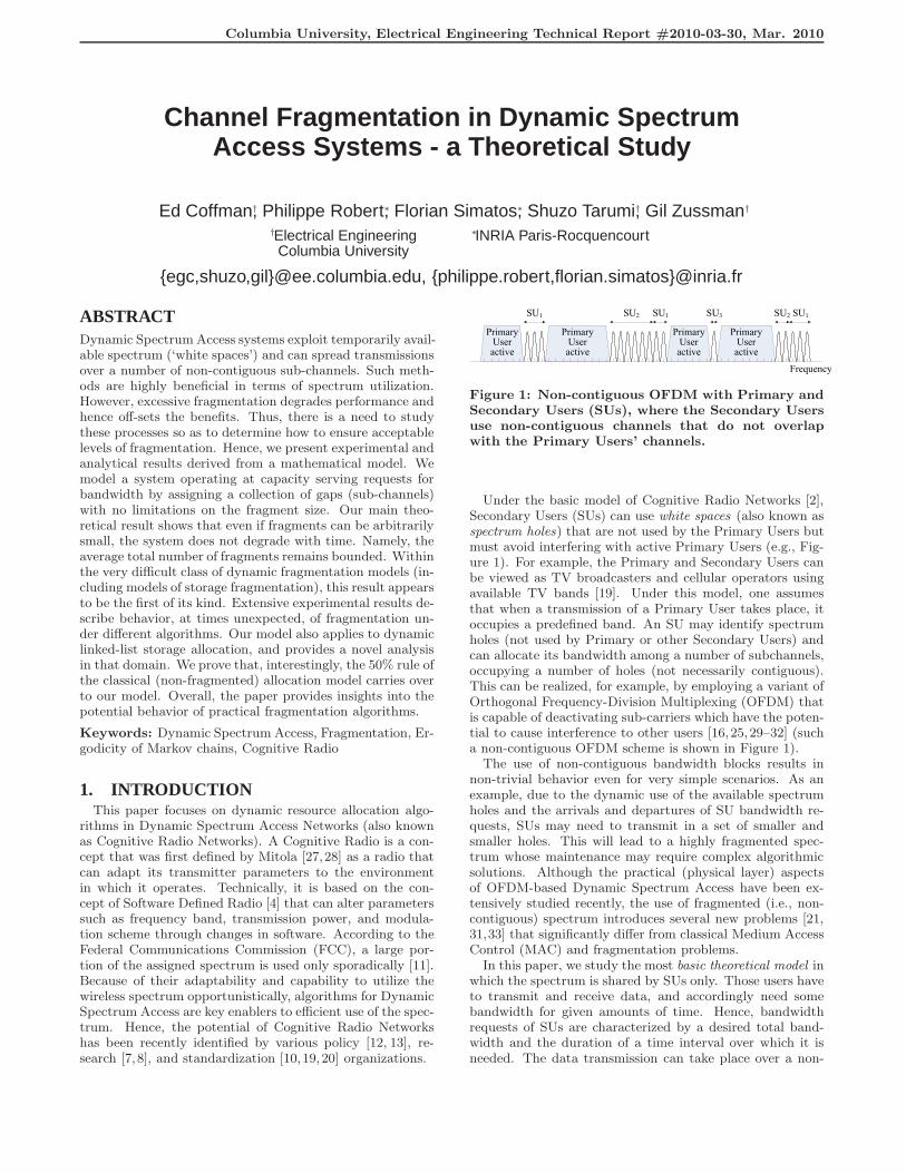
Figure 1: Non-contiguous OFDM with Primary andSecondary Users (SUs), where the Secondary Usersuse non-contiguous channels that do not overlapwith the Primary Users’ channels.

Under the basic model of Cognitive Radio Networks [2],Secondary Users (SUs) can use white spaces (also known asspectrum holes) that are not used by the Primary Users butmust avoid interfering with active Primary Users (e.g., Fig-ure 1). For example, the Primary and Secondary Users canbe viewed as TV broadcasters and cellular operators usingavailable TV bands [19]. Under this model, one assumesthat when a transmission of a Primary User takes place, itoccupies a predefined band. An SU may identify spectrumholes (not used by Primary or other Secondary Users) andcan allocate its bandwidth among a number of subchannels,occupying a number of holes (not necessarily contiguous).This can be realized, for example, by employing a variant ofOrthogonal Frequency-Division Multiplexing (OFDM) thatis capable of deactivating sub-carriers which have the poten-tial to cause interference to other users [16,25,29–32] (sucha non-contiguous OFDM scheme is shown in Figure 1).

The use of non-contiguous bandwidth blocks results innon-trivial behavior even for very simple scenarios. As anexample, due to the dynamic use of the available spectrumholes and the arrivals and departures of SU bandwidth re-quests, SUs may need to transmit in a set of smaller andsmaller holes. This will lead to a highly fragmented spec-trum whose maintenance may require complex algorithmicsolutions. Although the practical (physical layer) aspectsof OFDM-based Dynamic Spectrum Access have been ex-tensively studied recently, the use of fragmented (i.e., non-contiguous) spectrum introduces several new problems [21,31,33] that significantly differ from classical Medium AccessControl (MAC) and fragmentation problems.

In this paper, we study the most basic theoretical model inwhich the spectrum is shared by SUs only. Those users haveto transmit and receive data, and accordingly need somebandwidth for given amounts of time. Hence, bandwidthrequests of SUs are characterized by a desired total band-width and the duration of a time interval over which it isneeded. The data transmission can take place over a non-

contiguous channel (i.e., a number of subchannels). Once atransmission terminates, some fragments (subchannels) arevacated, and therefore, gaps (spectrum holes/white spaces)develop randomly in both size and position.

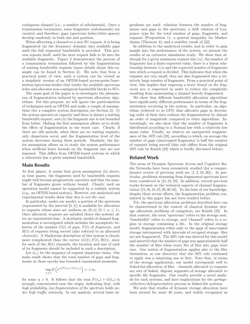
When allocating a channel to a new SU request, it is beingfragmented (in the frequency domain) into available gapsuntil the full requested bandwidth is provided. This pro-cess repeats itself, until the next request fails to fit into theavailable fragments. Figure 2 demonstrates the process ofa transmission termination followed by the fragmentationof waiting bandwidth requests (more details about this ex-ample can be found in Section 2). We note that from apractical point of view, such a system can be viewed asa simplistic version of an OFDM-based access-point/base-station/spectrum-broker that tracks the available spectrumholes and allocates non-contiguous bandwidth blocks to SUs.

The main goal of the paper is to investigate the phenom-ena of fragmentation induced by spectrum allocation algo-rithms. For this purpose, we will ignore the particularitiesof techniques such as OFDM and make a couple of assump-tions (for a complete system description, see Section 2): (i)the system operates at capacity and there is always a waitingbandwidth request; and (ii) the fragment size is not boundedfrom below. Making the first assumption allows us to studythe effect of fragmentation in the worst case. Clearly, ifthere are idle periods, when there are no waiting requests,only departures occur and the fragmentation level of thesystem decreases during these periods. Similarly, the lat-ter assumption allows us to study the system performancewhen artificial lower bounds on the fragment size are notimposed. This differs from OFDM-based systems in whicha subcarrier has a given minimal bandwidth.

Main ResultsAt first glance, it seems that given assumption (ii) above,as time passes, the fragments used by bandwidth requestsmight well become progressively narrower and that the num-ber of fragments grows without bound. Clearly, such anoperation model cannot be supported by a realistic system(e.g., an OFDM-based system). However, our analytical andexperimental results show that this is not the case.

In particular, under our model, a portion of the spectrum(represented by the interval [0, 1]) is available for allocationto requests whose sizes are uniform on (0, α] (0 < α ≤ 1).Once allocated, requests are satisfied (leave the system) af-ter an exponential time. A stochastic model of channel frag-mentation is investigated which includes the asymptotic be-havior of the number G(t) of gaps, F (t) of fragments, andR(t) of requests being served (also referred to as allocatedchannels). A Markovian description of this system is clearlymore complicated than the vector (G(t), F (t), R(t)), sincefor each of the R(t) channels, the location and size of eachof its fragments should be included in such a description.

Let (tn) be the sequence of request departure times. Ourmain result shows that the total number of gaps and frag-ments at these epochs has bounded exponential moments,

supn≥1

E

(

eη(F (tn)+G(tn)))

< +∞,

for some η > 0. It follows that the sum F (tn) + G(tn) isstrongly concentrated near the origin, indicating that, withhigh probability, low fragmentation of the spectrum holds un-der high traffic intensity. In our analysis, several basic in-

gredients are used: relations between the number of frag-ments and gaps in the spectrum; a drift relation of Lya-punov type for the total number of gaps, fragments, andrequests (Proposition 1); a general inequality for Markovchains (Theorem 4); and a stability result of [22].

In addition to the analytical results, and in order to gaininsight into the performance of the system, we present theresults of an extensive simulation study. We show that al-though for a given maximum request size (α), the number offragments has a finite expected value, there is a linear rela-tionship between 1/α and the expected number of fragmentsinto which a request is divided. This indicates that when therequests are very small, they are also fragmented into a rel-atively large number of fragments. From a practical point ofview, this implies that imposing a lower bound on the frag-ment size is important in order to reduce the complexityresulting from maintaining a channel heavily fragmented.

We show that different bandwidth allocation algorithmshave significantly different performance in terms of the frag-mentation occurring in the system. In particular, an algo-rithm (referred to as LFS) that allocates gaps in decreas-ing order of their sizes reduces the fragmentation by almostan order of magnitude compared to other algorithms. In-terestingly, we also show that the number of fragments isdistributed according to a Normal law with a relatively lowmean value. Finally, we observe an unexpected reappear-ance of the 50% rule [23], according to which, on average thenumber of gaps (unoccupied fragments) is half the numberof requests being served (this rule differs from the original50% rule by Knuth [23] which is briefly discussed below).

Related WorkThe areas of Dynamic Spectrum Access and Cognitive Ra-dio Networks have been extensively studied (for a compre-hensive review of previous work see [1, 2, 24, 26]). In par-ticular, problems stemming from fragmented spectrum havebeen considered in [21,31,33]. In addition, several previousworks focused on the technical aspects of channel fragmen-tation [15,16,18,25,29,30,32]. To the best of our knowledge,despite these recent efforts, the fragmentation problem con-sidered in this paper has not been studied before.

Yet, the spectrum allocation problems described here canbe characterized in the context of classical dynamic stor-age allocation problems of computers, see Knuth [23]. Inthat context, the term “spectrum” refers to the storage unit,“bandwidth” refers to storage, and “channel” refers to a re-gion in storage containing a file. In the original storagemodel, fragmentation refers only to the gaps of unoccupiedstorage interspersed with intervals of occupied storage: filesare not fragmented. The 50% rule was derived for this modeland asserted that the number of gaps was approximately halfthe number of files when exact fits of files into gaps wererare. Our notion of fragmentation applies also to the filesthemselves, so our discovery that the 50% rule continuedto apply was a surprising one at first. Note that, in termsof the storage application, our model corresponds well tolinked-list allocation of files – channels allocated to requestsare sets of linked, disjoint segments of storage allocated tospecific file fragments. Our results provide a novel analy-sis for such systems, and have implications for the garbage-collection/defragmentation process in linked-list systems.

We note that studies of dynamic storage allocation havebeen around for some 40 years, and widely recognized as

u1 u2 u3

x u4 u4

Waiting Request State of the Spectrum Next Departure

t1 : u4 = .35

u5 = .50

.25 .15 .30 .30

0

u5 u5

u4

u2

u1 u3t2 :.20.30.25 .15

u5 = .50 u1 u3t3 :.30.30.25 .15

.10

u6 = .15

u1

u3

t5 :

.20.30.40 .10

u5 u5u8 = .40 u7u7

.15.25.40 .10u6

.05

u5 u5u7 = .25 u3u3

.15.30.40 .10u6

.05t4 :

1

x.05

Figure 2: An example of the admission and departure processes and the resulting spectrum fragmentation.

posing very challenging problems to both combinatorial andstochastic modeling and analysis. In particular, results ofthe type found in this paper, rigorous within stochastic mod-els, seem to be quite new.

For a system without fragmentation, the early results ofKipnis and Robert [22] concern a stochastic analysis of thenumber of requests being served in the system. Fragmen-tation is not an issue in their case since request allocationscan be moved when needed in order to put available spaceall together in one block. A major result in [22] applying toour model asserts the existence and uniqueness of an invari-ant measure for the number of requests. Explicit formulasfor our system are hard to come by, but those in [22] forthe maximal departure rate in special cases have provideduseful checks on our experiments.

Organization of the PaperThe remainder of this paper is organized as follows. Sec-tion 2 describes the system, allocation algorithm, and themathematical variables describing fragmentation. Section 3presents simulation results that bring out the behavior ofthe system and the effects of fragmentation. Section 4 in-troduces some relations between the variables describing thefragmentation and a 50% limit law for the relation betweenthe number of active channels and the number of gaps in thespectrum at departure times. Section 5 contains our mainmathematical result, Theorem 2, which shows that the av-erage value of the total number of fragments and gaps isbounded. Furthermore, in some cases, the existence of anequilibrium distribution is established in Theorem 3. Sec-tion 6 discusses algorithmic issues, such as changes in perfor-mance resulting from alternative algorithms for sequencingthrough the list of gaps when constructing a channel for anewly admitted request. Section 7 presents experiments sug-gesting that Normal approximations for the total number offragments and gaps hold. Section 8 discusses the results andfuture research directions.

2. THE MODEL

System ModelAs mentioned above, we consider requests for bandwidthqueued up waiting to be served, each of them identified withthe amount of bandwidth required and a time telling howlong it wants a channel with that total bandwidth. Chan-nels are allocated to bandwidth requests on a FCFS (first-

come-first-served) basis, subject to available bandwidth; thechannels must remain fixed while active; they depart aftervarying delays, so gaps alternating with sequences of sub-channels (channel fragments) develop over time.

For convenience, we normalize the spectrum to the in-terval [0, 1], so all bandwidth requests are numbers in [0, 1].There is a queue of waiting requests that never empties. As-suming that the spectrum initially has no channels in use,the allocation process begins by allocating consecutive chan-nels i.e., consecutive subintervals of [0,1], to requests whosesizes are u1, u2, . . . until a request whose size ui, i > 1, isreached which exceeds available bandwidth, i.e.,

u1 + · · · + ui−1 ≤ 1 < u1 + · · · + ui

All i− 1 of the channels now begin their independent de-lays. Subsequent state transitions take place at departureepochs when the delays of currently allocated channels ex-pire. At such epochs, all fragments of the departing chan-nel are released. Suppose all requests up to uj have beenallocated channels and a request ui, i ≤ j, departs, releas-ing its allocated channel. Then uj+1, uj+2, . . . are allocatedtheir requested bandwidths until, once again, a request isencountered that asks for more bandwidth than is available.All channels then begin or continue their delays until thenext departure. A standard rule for setting up a channelis to scan the spectrum, from one end to the other, withgaps of available bandwidth allocated to fragments of thenew requested bandwidth until enough has been allocatedto satisfy the entire request. The last gap used in satisfyinga request is normally only partially used; the partial alloca-tion in the last gap is left-justified in that gap. We refer tothis scanning rule as Linear Scan.

An example is shown in Figure 2. Allocations for thefirst 8 user requests whose sizes are u1, · · · , u8 are shown,assuming that, at time 0, the spectrum is not in use. Therequests with sizes u1, u2, and u3 are the first to be allocatedchannels; u4 must wait for a departure, since the first 4request sizes sum to more than 1. The variables ti givethe sequence of departure times of allocated requests. Wesee that the first occurrence of fragmentation takes place atthe departure of u2 and the subsequent admission of u4; aninitial fragment of u4 is placed in the gap left by u2 and afinal fragment is placed after u3. Note also that, even afteru2 and u4 have departed, there is still not enough bandwidthfor u5. After the additional departure of u1, both u5 andu6, but not u7, can be allocated bandwidth.

In Section 6, we shall also evaluate two alternatives to the

Linear Scan rule: a Circular Scan, by which each linear scanstarts where the previous one left off, and a Largest-FirstScan intended to further reduce fragmentation. Althoughthese algorithms make different scans of the gap sequence,they are all alike in their treatment of the last gap occupied:the last fragment is left justified in the last gap. This is akey assumption, and it is very likely to hold in practice.

The allocation process described in this section contrastswith the classical model of dynamic storage allocation, inwhich each bandwidth request must be accommodated by asingle, sufficiently large gap of available spectrum. However,the process does correspond closely to the linked-list modelof dynamic storage allocation, in which an available-spacelist is maintained and files can be fragmented in accordancewith this list. This paper also yields a novel stochastic anal-ysis of such systems. Note that the assumption that there isalways another request in queue models a system operatingat capacity, where the departure rate, which is equal to theadmission rate, is often called maximum throughput.

Notation, State Space, and Probability ModelWe denote by U the size of the request waiting to be allo-cated bandwidth, and by Ui for i ≥ 1 the size of the ithrequest behind it. Except in the proof of Theorem 3 in Sec-tion 5, we omit the dependency in time of these variables forthe sake of notation. As mentioned in Section 2, we denoteby R(t) the number of channels (requests that are allocatedbandwidth) at time t. F (t) and G(t) denote the numberof fragments and gaps at time t. A Markovian descriptionof this system is clearly more complicated than the vector(G(t), F (t),R(t)). Hence, we now define the state space ofthe fragmentation process. At a given state, we denote byr the number of channels (requests to which bandwidth hasbeen allocated) and by si (1 ≤ i ≤ r) the amount of band-width allocated to these requests. A state of the spectrum[0, 1] carries the information given by a sequence in whichgaps alternate with sets of contiguous fragments:

Definition 1. A state x in the state space S of the frag-mentation process is denoted by

x = (L1, . . . , Lr;u)

where u is the size of (amount of bandwidth required by) therequest waiting at the head of the queue and Li, is the listof open subintervals of [0, 1] occupied by the fragments ofthe i-th channel. For x to be admissible, the open intervalsin ∪iLi must be mutually disjoint, and, since the size of uexceeds the bandwidth available, u > 1 − ∑

i si has to hold.

Note that for a specific state, the size of the requests inthe queue are denoted by u and uj , j ≥ 1 and the size of thechannels (requests that are already allocated bandwidth) aredenoted by si, 1 ≤ i ≤ r.1

Let (X(t)) be the process living in the state space S . Inthe probability model used in this paper, the bandwidth re-quests (Ui) are independent random variables which are uni-formly distributed on (0, α], 0 < α ≤ 1, and request res-idence times are i.i.d. mean-1 exponentials.2 Under thisprobability model, (X(t)) is a Markov process on S .

1For simplicity of the presentation, we did not use the no-tation si in the example provided in Figure 2.2The assumption that request sizes are uniformly dis-tributed is for convenience. The results hold for more generaldistributions.

100 200 300 400 500 600 700 800 900 10000

200

400

600

800

1000

1200

1400

1600

1800

2000

1/α

Num

ber

Number of ChannelsNumber of Fragments per ChannelNumber of Gaps

Figure 3: Average numbers of channels, of gaps, andof fragments per channel.

3. EXPERIMENTAL RESULTSIn this section we describe an experimental study of the

model described above. This serves two related roles. First,it brings out characteristics of the fragmentation processthat need to be borne in mind in implementations, par-ticularly where these characteristics show conditions (e.g.,parameter settings) that must be avoided, if a system withfragmentation is to operate efficiently. The second role isthat of experimental mathematics, in which results indi-cate where behavior might well be formalized and rigorouslyproved as a contribution to mathematical foundations. Inthe latter role, this section leads up to the next two sections,which formalize the stability of the fragmentation process.

The experiments were conducted with a discrete-eventsimulator written in C. In general, the tool is capable of sim-ulating stochastic request arrival/departure processes. Forthis paper, however, the arrival process was effectively in-operative, since the interest here is behavior while the sys-tem is operating at capacity (i.e., at maximum throughput).Admissions are made whenever the waiting request fits intoavailable spectrum, and once made the waiting request isimmediately replaced by another with independent samplesfrom the required-bandwidth and residence-time distribu-tions. The admission process continues in this way, effec-tively simulating a queue that never empties, until no fur-ther admissions can be made and one or more departuresneed to occur. The excellent accuracy of the tool was es-tablished in tests against exact queueing results, and exactresults from [22]. The verification details are omitted andcan be found in Appendix A.

Recall that bandwidth requests are uniformly distributedon (0, α], 0 < α ≤ 1. Hence, the principal parameter of theexperimental model will be α. The simulations of stationarybehavior were most demanding, of course, for small α. Forevery α value, 0.01 ≤ α ≤ 1, 20 million departure eventswere simulated starting in an empty state, with data col-lected for the last 10 million events. For 0.001 ≤ α ≤ 0.01,100 million departure events were processed and data col-lection was performed during the last 50 million events.

The results for the average number of channels, the aver-age number of gaps, and the average number of fragmentsper channel are shown in Figure 3. The curves are nearlylinear in 1/α (the errors in the linear fits are within thethickness of the printed lines). In particular, the asymptotic

100 200 300 400 500 600 700 800 900 10000

0.5

1

1.5

2

2.5

3

x 106

1/α

Num

ber

of F

ragm

ents

Figure 4: Average total number of fragments vs.1/α: a quadratic fit.

0 0.1 0.2 0.3 0.4 0.5 0.6 0.7 0.8 0.9 10

0.1

0.2

0.3

0.4

0.5

0.6

0.7

0.8

0.9

1

α

Pro

port

ion

Type−0 fragmentType−1 fragmentType−2 fragment

Figure 5: Percentage of type-i fragments.

average number of channels in the spectrum is 2/α. Whenrequests are large relative to the spectrum (i.e., for α > 1/3),the behavior is not given by functions quite so simple. Assuch cases are of less practical interest, we omit the relevantdata due to space constraints.

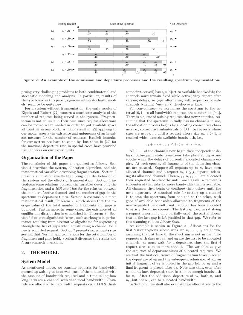
The asymptotic linear growth of the average number ofchannels as a function of channel size is obvious, but thelinearity of the other two measures is not so obvious. Acloser look shows that the average number of gaps is almostexactly one half the average number of channels for even rel-atively small 1/α. This is an unexpected version of Knuth’s50% rule for dynamic storage allocation. We return to thisbehavior in the next section, where we prove a 50% limitlaw. The linear growth of the average number of fragmentsper channel may also be unexpected at first glance: the frag-mentation of channels increases as the average channel sizedecreases. This linear growth implies the quadratic growthof the average total number of fragments plotted in Figure4 (the accuracy of the fit is as before: the error is within thethickness of the printed lines).

The analysis in the later sections will focus largely ontracking fragment types defined as follows: a fragment is oftype-i, if it is adjacent to 0, 1, or 2 fragments. It can be seenin Figure 5 that for small α, more than 90% of the fragmentsare type-2 fragments. In addition, clearly, the number oftype-0 and type-1 fragments is a function of the numberof gaps. These observations and the results illustrated in

0 0.1 0.2 0.3 0.4 0.5 0.6 0.7 0.8 0.9 10

0.1

0.2

0.3

0.4

0.5

0.6

0.7

0.8

0.9

1

α

Siz

e

Average Size of FragmentsAverage Size of Gaps

(a) 0 ≤ α ≤ 1

0 0.01 0.02 0.03 0.04 0.05 0.06 0.07 0.08 0.09 0.10

0.5

1

1.5

2

2.5

3

3.5

4

4.5

5x 10

−3

α

Siz

e

Average Size of FragmentsAverage Size of Gaps

(b) 0 ≤ α ≤ 0.1

Figure 6: Average sizes of fragments and gaps.

Figures 3 and 4 indicate that, even for relatively small 1/α,the average total number of type-0 and type-1 fragmentsgrows linearly in 1/α, but the average number of type-2fragments grows quadratically.

Figure 6 compares the average gap and fragment sizes. Asmight be expected, for relatively small α, they are close toeach other. The relation holds even for moderately large α,although for α rather close to 1, the difference amounts toabout a factor of 2. With this property and the 50% rulesuggested by Figure 3, the linear growth in the number offragments per channel (shown in Figure 3) is easily explainedfor moderately small α in the following way.

As mentioned above, for moderately small α, the numberof channels is approximately 2/α (i.e., the spectrum size di-vided by the average request size). Due to the 50% rule, thenumber of gaps is roughly 1/α. At any time, the total size ofthe gaps is at most α, since there is a request waiting for de-partures whose requested bandwidth exceeds that total sizeof gaps. Therefore, at most α available bandwidth is spreadamong 1/α gaps, giving an average gap size on the order ofα2. The average fragment size is at most (and indeed veryclose to) the average gap size. The fragments must occupyat least 1−α of the spectrum (since, as mentioned above, atmost a fraction α of the spectrum is devoted to gaps). Thus,the number of fragments must be on the order of 1/α2, andso the average number of fragments per channel must be onthe order of (in particular, linear in) 1/α. As α → 0, theasymptotics of these estimates become more precise.

4. NUMBERS OF FRAGMENTS AND GAPSAs mentioned in Section 2, under our probability model,

(X(t)) (the process living in the state space S) is a Markovprocess on S . In this section, we obtain analytical resultsregarding the number of fragments and gaps under this pro-cess. We begin by formally defining the fragment typeswhich were discussed in Section 3.

Definition 2. For i = 0,1, or 2, a fragment is said to beof type i if it touches exactly i other fragments. Ni(t) denotesthe number of type i fragments at time t, so that F (t) =N0(t) +N1(t) +N2(t) is the total number of fragments.

Let σ(t) denotes the sum of the number of fragments andgaps,

σ(t) = F (t) +G(t). (1)

The numberG(t) of gaps and the numbers of fragment typesare related as follows.

Lemma 1. With probability 1,

G(t) = N0(t) +1

2N1(t) + I(t) (2)

For any t ≥ 0, where I(t) = 1, if there is a gap starting atthe origin, and 0 otherwise.

Proof. Each gap, except for boundary gaps starting at0 or ending at 1, separates two fragments. Two gaps sur-round a type-0 fragment not touching the origin, only onetouches a type-1 fragment not touching the origin, and nonetouch a type-2 fragment, so the gaps strictly inside (0, 1)are double-counted in 2N0(t) +N1(t). Gaps at the bound-aries are counted only once in this expression, so if there aregaps touching each boundary, 2 must be added to 2N0(t) +N1(t) to produce a double count of all gaps. Then N0(t) +N1(t)/2 + 1 counts the gaps as called for by the lemma.

With probability 1, a gap always touches the boundary at1, so the only case left to consider is the absence of a gaptouching the origin. In this case, there is a type-0 or type-1fragment touching the origin, and so a nonexistent gap hasbeen counted in 2N0(t)+N1(t). This over-count cancels theunder-count of the gap touching 1, and so no correction termis needed, i.e., N0(t) +N1(t)/2 counts all gaps as stated inthe lemma.

Definition 3. Let (tk) denote the sequence of departuretimes, let Di(tk) denote the number of type i fragments in thechannel leaving at time tk, and let A(tk) denote the numberof requests admitted to the spectrum at time tk. Finally,define the drift in the total number of fragments and gaps:

∆σ(tk)def= σ(tk) − σ(tk−1). (3)

The following lemma is the basis of the stability analysisof σ(t) in Section 5, and the 50% rule proved later in thissection.

Lemma 2. With probability 1, the departure at tk createsthe following change in the total number of fragments andgaps:

∆σ(tk) = A(tk) − 2D0(tk) −D1(tk) + J(tk), k ≥ 1 (4)

with t0 = 0, and J(tk) = 1, if a fragment starting at theorigin is in the departing channel, and 0 otherwise.

Proof. With probability 1, each new channel allocationcovers completely every gap it is allocated, except for the lastone, which is only partially covered. Thus, with probability1, each new channel allocation changes gaps to fragments,except for the last gap which is changed to a fragment plusa gap; this adds one to σ(tk−1) for each admission, whichaccounts for the total of A(tk) in (4).

Two fragments of the same channel can not be contiguous,so it is correct to add up the changes created by departingfragments, with each being treated separately. Suppose firstthat there is no fragment (0, b) against the origin. Then forevery type-0 fragment in the departing channel, two gapsand a fragment are replaced by a single gap for a net de-crease of two, and for every departing type-1 fragment, agap and a fragment are replaced by a single gap for a net re-duction of one. This gives the reduction of 2D0(tk)+D1(tk)appearing in (4). If there is a fragment (0, b), it must beof type 0 or 1; if it is of type 0, then its departure gives adecrease of one; if it is of type 1, its departure has no effect.Each of these contributions is one less than it would be werethe fragment not touching the origin. There can only beone such fragment, so the correction shown in J(tk) for afragment (0, b) follows.

We will denote by G−(tk) the total number of gaps justafter the k-th departure, but before new admissions, if any,are made. Note that if we remove A(tk) from the right-handside of (4) and add back the total number of departing frag-ments at tk, i.e., D0(tk)+D1(tk)+D2(tk), we get the numberof gaps available to admissions at the k-th departure:

G−(tk) = G(tk−1) −D0(tk) +D2(tk) + J(tk) (5)

with J(tk) = 1, if there is a departing fragment (0, b), and 0otherwise.

Knuth’s widely known 50% rule appears in a very differentcontext than the model here, so it is difficult to anticipate theapparent fact that it also holds for our fragmentation model.However, one can argue a similar result assuming only thatthe fragmentation process has a stationary distribution. Theresult is given below as an expected value of a ratio, ratherthan a ratio of expected values.

Theorem 1. Assume that the fragmentation process atdeparture epochs tk has the stationary distribution πα, thenas α→ 0,

Eπα

(

G(tk)

R(tk)

)

∼ 1

2

Proof. In the stationary regime, one has, by Lemma 2,

Eπα[σ(tk) − σ(tk−1)] =

Eπα[A(tk) − 2D0(tk) −D1(tk) + J(tk)] = 0,

and to balance departure and admission rates, we must haveEπα

A(tk) = 1. Thus, we can write

Eπα[2D0(tk) +D1(tk) − J(tk)] = 1. (6)

Now for a state x at time tk having r channels and Ni(tk)type-i (i = 0, 1, 2) fragments, we have from Lemma 1

Ex[2D0(tk) +D1(tk) − J(tk)] =

(2N0(tk) +N1(tk))/r − Ex[J(tk)] =

2[G(tk) − I(tk)]/r − Ex[J(tk)] = 2G(tk)/r +O (1/r)

Thus, dropping the O(1/r) term that tends to 0 with α uni-formly in x, the expectation in (6) proves the theorem.

5. STABILITY RESULTSThis section establishes that the average total number of

fragments and gaps remains bounded and that, for certaindistributions of request sizes, ergodicity holds. The analysisleads to the two following results. Recall that (tn) is thesequence of departure times (t0 = 0) and σ(t) = F (t)+G(t),defined in (1), is the total number of fragments and gaps.

Theorem 2. There exists some η > 0 such that, for anyinitial state x ∈ S,

supn≥1

Ex

(

eησ(tn))

< +∞. (7)

Clearly, this implies that for any initial state x ∈ S , thesequence (Ex(σ(tn)), n ≥ 0) is bounded. With an additionalassumption on the distribution of the request size, a strongerstability result can be proved.

Theorem 3. When α > 1/2, the process (X(t)) is posi-tive Harris recurrent; in particular, it has a unique station-ary distribution.

A criterion for finite exponential moments using a Lyapunovfunction is established next. Then, we provide some esti-mates of the drift of the number of fragments between de-partures which will show us how to construct a Lyapunovfunction. After constructing this function, we will be in po-sition to prove the boundedness of exponential moments.

A Criterion for Finite Exponential MomentsBefore stating the main result, some results on Markov chainsare needed. In the sequel, ≤st refers to stochastic ordering,i.e., V ≤st Z means that E(f(V )) ≤ E(f(Z)) for any in-creasing function f . For reasons that will become clear inLemma 5, the following lemma focuses on admissions at 4consecutive departure times. Recall that (Ui, i ≥ 1) are thesizes of the requests waiting to be allocated bandwidth (afterthe first one U), which are assumed to i.i.d.

Lemma 3. The random variable A(t1) + · · · + A(t4) isstochastically dominated by a random variable Z such thatE(eλZ) < +∞ for some λ > 0.

Proof. It is clear that A(t1) ≤ Z + 1 where

Z = 1 + inf{n ≥ 1 : U1 + · · · + Un ≥ 1}.The Markov inequality shows that for any z ≥ 0,

P(Z ≥ z + 1) = P(U1 + · · · + Uz ≤ 1) ≤ e(

E

(

e−U1

))z

and so E(eηZ) is finite for η > 0 small enough. From thisobservation, it is not difficult to extend the result to A(t1)+· · · + A(t4) instead of just A(t1).

This lemma shows in particular that

ξdef= sup

i≥1supx∈S

Ex(A(ti)) < +∞.

is well-defined; this constant will be used repeatedly through-out the rest of the analysis. The proof of the following lemmais standard, and therefore, omitted.

Lemma 4. Let Z ≥ 0 be a positive, real-valued randomvariable such that E(eλZ) < +∞ for some λ > 0, and definec = λ−2

E(eλZ − 1 − λZ). Then for any 0 ≤ ε ≤ λ and anyreal-valued random variable V such that V ≤st Z, we haveE

(

eεV)

≤ 1 + εE(V ) + ε2c.

The following result is closely related to result of Hajek [17].The proof can be found in Appendix B.

Theorem 4. Let (Yk) be a discrete-time, continuous state-space Markov chain such that for some function f ≥ 0,there exist K, γ > 0 such that for any initial state y withf(y) > K, Ey(f(Y1)−f(Y0)) ≤ −γ. Assume that there existsa random variable Z such that for any initial state y, Z dom-inates stochastically the random variable f(Y1) − f(Y0) un-der Py. Assume finally that E(eλZ) < +∞ for some λ > 0.Then there exist η > 0 and 0 ≤ C < +∞ such that for anyinitial state y,

supn≥1

Ey

(

eηf(Yn))

≤ eηf(y) + C.

Theorem 4 will be applied to the Markov chain (X(t4n))with a function f of the form σκ = σ + κr for some κ > 0suitably chosen. (X(t4n)) is not the most natural choiceat first glance, but it appears to be needed because of thecomplexity of the state space.

It is clear that σ(t1) − σ(t0) ≤ A(t1) + 1, so that

σκ(t4) − σκ(t0) ≤ (κ+ 1)(A(t1) + · · · +A(t4)) + 4

and therefore, by Lemma 3, σκ(t4)−σκ(t0) is stochasticallydominated by some random variable Z with an exponentialmoment. Therefore, one has to establish a negative drift re-lation for σκ(t4)−σκ(t0). This is the purpose of the followingtwo subsections.

Evolution of the Number of FragmentsRecall that x ∈ S , the initial state of the system, has r ac-tive channels, and define the total available gap size h =1− (s1+ · · ·+sr). Time 0 referring to the initial state x willusually be omitted; e.g., σ(0), F (0), G(0), . . . will be simpli-fied to σ, F,G, . . .. Recall that ∆σ(tn) is defined in (3) asσ(tn) − σ(tn−1).

Lemma 5. Fix 0 < ε < 1 and 0 < η < 1/2, and let x ∈ Sbe an initial state such that σ = G+ F ≥ 2K + 1 for somefixed K ≥ 0.

Then F = N0 +N1 +N2 ≥ K, and

1) If r = 1, then Ex(∆σ(t1)) ≤ ξ −K.

2) If r > 1 and N0 +N1 ≥ εK, then

Ex(∆σ(t1)) ≤ ξ + 1 − εK

r.

Assume in the remaining cases that r > 1, define K′ =

K(

(1 − ε)/r − ε)+

, and let i∗ ∈ {1, . . . , r} index a channelLi∗ in x with the most type-2 fragments.

3) If N0 +N1 ≤ εK and u > h+ si∗ , then

Ex(∆σ(t2)) ≤ ξ + 2 − K′

r(r − 1). (8)

4) If N0 +N1 ≤ εK, u < h+ si∗ and h+ si∗ < ηα, then

Ex(∆σ(t3)) ≤ ξ + 2 − (1 − η)K′

r2(r − 1). (9)

5) If N0 +N1 ≤ εK, u < h+ si∗ and ηα < h+ si∗ , thenthere exists a γ(η) > 0 such that

Ex(∆σ(t4)) ≤ ξ + 2 − γ(η)K′

r5. (10)

It follows that there exists a ξ > 0 and a function ψ(r) > 0such that for any x with σ ≥ 2K + 1,

Ex(σ(t4) − σ) ≤ ξ −Kψ(r). (11)

Proof. As is readily verified, G ≤ F + 1, so 2K + 1 ≤σ = F +G ≤ 2F +1, and hence F ≥ K as claimed. In whatfollows, we use repeatedly the two following simple facts:

Ex (D0(t1) +D1(t1)) = (N0 +N1)/r, (12)

and by Lemma 1,

G ≥ K ⇒ N0 +N1 ≥ K − 1. (13)

— First case: r = 1. Then, right after the only channelinitially present leaves, there is no channel allocated band-width, and therefore, σ(t1) = A(t1). Note that r = 1 is onlypossible when α > 1/2, and in this case the possibility fora channel to be alone is crucial in the proof of the Harrisrecurrence stated in Theorem 3.— Second case: r > 1, N0 +N1 ≥ εK. Then the inequalityfollows from (4):

Ex(∆σ(t1)) ≤ ξ + 1 − Ex(D0(t1) +D1(t1))

= ξ + 1 − N0 +N1

r≤ ξ + 1 − εK

r.

In the 3 remaining cases, let N∗j denote the number of

type-j fragments in any channel i∗ which has the most type-2fragments. If N0 +N1 ≤ εK, then since F ≥ K, necessarilyN2 ≥ (1 − ε)K and N∗

2 ≥ (1 − ε)K/r. Define the eventD∗ = {channel Li∗ leaves at t1} and recall that G− denotesthe number of gaps right after Li∗ leaves but before newadmissions, if any, are made. It follows from (5) that G− ≥K′ in the event D∗, since

G− = G−N∗0 +N∗

1 + J(t1) ≥ (−εK + (1 − ε)K/r)+ = K′.

The remaining analysis tacitly assumes that r > 1, thatN0 +N1 ≤ εK and that the channel Li∗ leaves at t1.— Third case: u > h+ si∗ . Then A(t1) = 0, since when Li∗

leaves it does not provide enough additional bandwidth for U .In particular, R(t1) = r − 1 and G(t1) = G− ≥ K′, and so

Ex(∆σ(t2)) ≤ ξ + 1 − Ex(D0(t2) +D1(t2);D∗).

The strong Markov property makes it possible to lower-bound this last term.

Ex(D0(t2)+D1(t2);D∗) = Ex(EX(t1)(D0(t1)+D1(t1));D

∗)

= Ex

(

(N1 +N2)(t1)

R(t1);D∗

)

≥ K′ − 1

r − 1Px(D∗) =

K′ − 1

r(r − 1)

and therefore, Ex(∆σ(t2)) ≤ ξ + 2 −K′/(r(r − 1)).— Fourth case: u < h+si∗ < ηα. In this case U is admittedat t1. Thus it makes sense to define the event

E4 = D∗ ∩ {U leaves at t2 and U1 > ηα}.Then as before

Ex(∆σ(t3)) ≤ ξ + 1 − Ex(D0(t3) +D1(t3);E4).

In the event E4, U is admitted at t1 and leaves at t2, whileU1 stays blocked at t1 and t2, so that G(t2) = G− ≥ K′ andR(t2) = r − 1. Hence as in the second case,

Ex(D0(t3) +D1(t3);E4) ≥ K′ − 1

r − 1Px(E4) ≥ (1 − η)K′

r2(r − 1)− 1

since Px(E4) = (1 − η)/r2. Thus (9) holds.— Fifth case: u < h + si∗ and ηα < h + si∗ . Again, U isadmitted at t1. Letting Ui denote the sizes of the requestsbehind U , define the event

B = {Ui < ηα, i = 1, . . . , τ and Uτ+1 > 2ηα}with τ = inf{n ≥ 0 : U1 + · · · + Un > h + si∗ − ηα} andE′

5 = D∗ ∩ B ∩ {U leaves at t2}. It is readily verified that1 ≤ τ < +∞ almost surely. Moreover, one has in E′

5

0 < h∗ def= h+ si∗ − (U1 + · · · + Uτ ) < ηα < Uτ+1.

This means that at t2, exactly τ new requests U1, . . . , Uτ

have been admitted, and Uτ+1 is blocked. Moreover, forany i ∈ {1, . . . , τ}, one has h∗ + Ui < 2ηα < Uτ+1, so thatif one of the τ channels allocated to the (Ui) leaves, Uτ+1

remains blocked.When Li∗ left, there wereG− ≥ K′ gaps; in the remainder

of the analysis, we call an initial gap a gap present rightafter Li∗ left. After Li∗ left, U and A(t1) − 1 new requestswere admitted, and then U left and A(t2) new requests wereadmitted at t2. Thus, at t2, each initial gap is in either oftwo states: either it is completely filled, or it is still a gap,i.e., it has not been filled completely. Let k be the number ofinitial gaps completely filled at t2, and let k′ = G−−k: thenk+ k′ = G− ≥ K′. In each initial gap completely covered att2, there is at least one type-2 fragment of one of the τ newchannels. Therefore, N1,2 +N2,2 + · · · +Nτ,2 ≥ k with Ni,2

the number of type-2 fragments of the channel correspondingto U . In particular there is a channel Lj∗ , j

∗ ∈ {1, . . . , τ}with at least the average k/τ of type-2 fragments: Nj∗,2 ≥k/τ . Define finally the event E5 = E′

5 ∩ {Lj∗ leaves at t3}.Since h∗ + Uj∗ < Uτ+1, then Uτ+1 remains blocked at t3when E5 occurs, and therefore (note that when j∗ leaves,some gaps may merge, but not two initial gaps),

G(t3) ≥ Nj∗,2 + k′ ≥ k/τ + k′ ≥ (k + k′)/τ ≥ K′/τ.

Now we proceed as before, to obtain

Ex(∆σ(t4)) ≤ ξ + 1 − Ex(D0(t4) +D1(t4);E5)

and, using the Markov property at time t3,

Ex(D0(t4)+D1(t4);E5) = Ex(EX(t3)(D0(t1)+D1(t1));E5)

= Ex

(

(N0 +N2)(t3)

R(t3);E5

)

≥ Ex

(

(K′/τ − 1)+

r + τ − 2;E5

)

since R(t3) = r + τ − 2 in E5. The same kind of reasoningas before then leads to

Ex

(

(K′/τ − 1)+

r + τ − 2;E5

)

≥ K′

r5f(η, h+ si∗ − αη) − 1

with the function f(η, ·) defined for y > 0 by

f(η, y) = E(

(1 + τ (y))−5;B(η, y))

with τ (y) = inf{n ≥ 1 : U1 + · · · + Un ≥ y} and

B(η, y) = {Ui < ηα, i = 1, . . . , τ (y) and Uτ(y)+1 > 2ηα}.It is not difficult to show that γ(η) = inf0<y<1 f(η, y) > 0which then gives the result.

It remains to prove (11). One only needs to assemble thevarious bounds, taking into account that Ex(∆σ(ti)) ≤ ξ+1for any x ∈ S and i ≥ 0, to arrive at 4 separate bounds onEx(σ(t4) − σ). For example, using the former bound for

the first two terms and the last term of Ex(σ(t4) − σ) =∑

1≤i≤4 Ex∆σ(ti) and then the bound in (9) for the thirdterm, we get that one of the 4 bounds, which applies whenx satisfies the inequalities of the fourth case, is

Ex(σ(t4) − σ) ≤ 4ξ + 5 − (1 − η)K′

r5

Computing the minimum over these bounds with η = 1/4and ε = 1/r2, one obtains (11) after setting ξ = 4ξ + 5 and

ψ(r) =ϕ(r)

r6× ((1 − η) ∧ γ)

with ϕ(r) = 1 − 2r−2. This concludes the proof.

We turn now to the case where r is large. In this case, thenegative drift comes from the fact that, except perhaps at t1,with high probability there is no admission at a departure,since the channel that leaves is small with high probability.However, we see in (4) that this is not enough for σ to decay,for one would need at least one type-0 or type-1 fragment toleave as well, and it can be the case that most fragments areof type-2. The second term of the Lyapunov function allowsus to get around this problem. Since the variation ∆R(tk)in the number of channels at a departure is exactly equal toA(tk) − 1, one readily gets that

σκ(t4) − σκ = (σ(t4) − σ) + κ(A(t1) + · · · + A(t4) − 4).

In particular, if x ∈ S is such that σ ≥ 2K + 1 and r ≤ Kr,then (from now on, we assume without loss of generalitythat the function ψ given by (11) in Lemma 5 is decreasing)

Ex(σκ(t4) − σκ) ≤ ξ −Kψ(Kr) + 4κ(ξ − 1)

whereas if r ≥ Kr,

Ex(σκ(t4) − σκ) ≤ 4(ξ + 1) + κEx(r(t4) − r)

and so we see that we only need to control Ex(r(t4)−r) for rlarge.

Lemma 6. There exist Kr, γr > 0 such that if x ∈ S issuch that r ≥ Kr, then Ex(r(t4) − r) ≤ −γr.

Proof. Since the technical difficulty of the proof of thisinequality is similar to that of the above proof, we need onlygive a sketch of it. From s1 + · · · sr = 1 − h ≤ 1 one gets#{i : si ≥ γ} ≤ 1/γ, and therefore, Px(si1 ≥ 1/

√r) ≤ 1/

√r

with Li1 , i1 ∈ {1, . . . , r}, the channel that leaves at t1. Thus,when r is large, with high probability a small channel leaves.

If h−u is away from α, then the event {u1 > h−u+si1 +· · · + si4} (with ik defined similarly) has high probability,and in this event A(t1) + · · · + A(t4) ≤ 1. If in contrasth−u is large, then with high probability U1 is admitted andwith high probability h − u− U1 is away from α; hence wecan do the same again, and get that, with high probability,A(t1) + · · · + A(t4) ≤ 2. The lemma is proved.

Construction of a Lyapunov FunctionFor κ > 0, one defines, for an initial state x ∈ S of the

system, σκdef= σ + κ r, where r is the number of channels

allocated in x and σ = F + G is the sum of the number offragments and gaps in x.

Proposition 1. (Lyapunov function inequality) There ex-ist κ and K > 0 such that if x ∈ S is such that σκ ≥ K,then Ex(σκ(t4) − σκ) ≤ −1.

Proof. Let Kr and γr be as in Lemma 6, and take κ andK as follows:

κ =4ξ + 5

γrand K =

8ξ + 2ξ + 2

ψ(Kr)+ κKr + 1.

Assume that σκ ≥ K. If r ≥ Kr, then

Ex(σκ(t4) − σκ) ≤ 4(ξ + 1) − κγr = −1.

Otherwise, r ≤ Kr, and since σκ ≥ K, this necessarily givesσ ≥ K − κKr = 2K̂ + 1 with K̂ = (K − κKr − 1)/2. Thus,

Ex(σκ(t4) − σκ) ≤ ξ − K̂ψ(Kr) + 4ξ = −1

and the proposition follows.

Proof of Theorem 2Theorem 4 and Lemma 3 applied to the Markov chain (X(t4n),n ≥ 0), and the function σκ show that for some η > 0 andsome constant 0 ≤ C < +∞,

supn≥0

Ex

(

eησκ(t4n))

≤ eησκ + C.

Then the Markov property gives for any i ≥ 0

supn≥0

Ex

(

eησκ(t4n+i))

≤ Ex

(

eησκ(ti))

+ C < +∞

from which (7) follows readily.

Proof of Theorem 3In the following discussion, no conceptual argument is miss-ing, only some formalism needed to handle the continuousstate space S . These details are routine and left to the in-terested reader. In the analysis below, requests are said tobe big if their size exceeds 1/2.

We argue that (X(t)) visits infinitely often a state in whichthere are no fragmented channels, and such that all sizedistributions remain the same at all visits. This is enoughto show Harris recurrence; see for instance Asmussen [3]. Forthis purpose, it is convenient to pick a simple regenerationset E ⊂ S in which (i) the spectrum is being used by abig request, alone and with an unfragmented channel of theform (0, b), and (ii) the request U waiting at the head of thequeue is also big. Each of these has the conditional request-size distribution given that its size is larger than 1/2, i.e.,the uniform distribution on (1/2, α), see [22].

To verify that E is visited infinitely often, consider theprocess (R(t), U(t)) with R(t) the number of requests allo-cated a channel at time t and U(t) the size of the requestat the head of the queue; the process (R(t), U(t)) is simplythe process (X(t)) when the data on fragmentation is ig-nored. This process is positive Harris recurrent, as shownin Kipnis and Robert [22]. In particular it visits infinitelyoften states with R(t) = 1 and U(t) > 1/2; one can addU1(t) > 1/2 as well (i.e., the first request in line behind thehead of the queue request is also big), since this happenswith a geometric probability. Then when the only channelleaves, the process (X(t)) enters E, since there is exactlyone channel, it is big, it is necessarily unfragmented and ofthe form (0, b), and a big request is waiting at the head ofthe queue. Moreover, this argument shows that the timebetween visits to E is integrable, which in turn establishespositive Harris recurrence. This completes the proof.

10 20 30 40 50 60 70 80 90 1000

20

40

60

80

100

120

140

160

180

200

1/α

Num

ber

of F

ragm

ents

per

Cha

nnel

Linear ScanCircular ScanLargest−First Scan

Figure 7: Average number of fragments per channel.

6. ALGORITHMSAlthough the focus so far has been on measures of frag-

mentation as a function of α, algorithmic issues are also ofobvious interest. For example, more uniform patterns ofgaps might be an advantage. The Linear Scan (LS), dis-cussed in the previous sections, tends to push the gaps to-wards the end of the spectrum, particularly when the spec-trum is viewed at random times in steady state. Interest-ingly, our experiments have shown that, for all α < 1/3, thestarting position of the first gap in the spectrum remainsvery close to 0.64.

To uniformize gap locations, an alternative gap scan re-sembles the Circular Scan (CS) sequences of dynamic stor-age allocation [23]. In our case, CS uses a circular gap list,in which the successor to the last gap in [0,1] is the first gapin [0,1]. The scan is still linear, but the starting gap of thescan moves as follows: if the last fragment of a channel isplaced in gap g, then the residual gap of g is the first gapscanned in constructing the next channel. Clearly, althoughCS will tend to uniformize gap sizes as a function of posi-tion, boundary effects will persist so long as the spectrumitself is not circular, i.e., gaps and fragments are not allowedto overlap the end of the spectrum, a restriction that wouldlikely be dictated in practice.

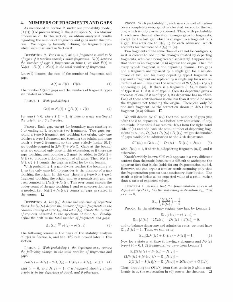
The average number of fragments per channel is a directmeasure of gap-search times, and one that we use here. Forvalues of α expected to be of interest in applications, theeffects of CS on gap-search times are only within a few per-cent relative to LS, as can be seen in Figure 7. The figurealso shows the average number of fragments per channel forthe Largest-First Scan (LFS) algorithm. This algorithm isdesigned to speed up the process of finding a set of gapssufficient to create a new channel. It selects available gapsin a decreasing order of their sizes and allocates them toa request, thereby greedily minimizing the number of gapsneeded to fulfill a request. The extra mechanism neededfor such a search will of course tend to reduce overall perfor-mance gains. The results in Figure 7 for LFS show a surpris-ingly large improvement in the average number of fragmentsper channel – as can be seen, a reduction by a factor morethan 3 is achieved by LFS for even moderately small α.

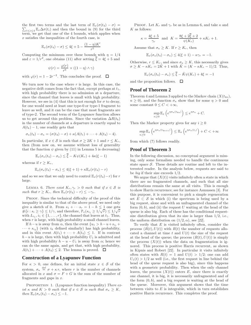
The Probability Mass Functions (pmf’s) of the number offragments per channel are shown in Figure 8. Notice thatwhile all probabilities are small under LS and CS, the largestapplies to the case of no fragmentation at all. The much

0 5 10 15 20 25 30 35 40 45 50 55 600

0.02

0.04

0.06

0.08

0.1

0.12

0.14

0.16

0.18

Number of Fragments per Channel

Pro

babi

lity

Mas

s F

unct

ion

Linear ScanCircular ScanLargest−First Scan

Figure 8: Distribution of the number of fragmentsper channel for α = 0.1.

0 0.1 0.2 0.3 0.4 0.5 0.6 0.7 0.8 0.9 1

0.5

0.6

0.7

0.8

0.9

1

α

G/R

Linear ScanLargest−First ScanCircular Scan

Figure 9: G/R → 1/2 as α → 0 under LS, LFS, andCS.

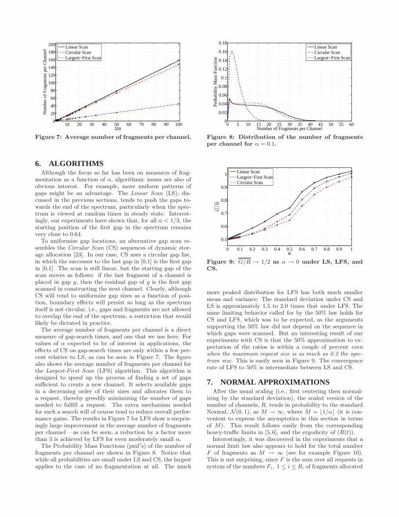
more peaked distribution for LFS has both much smallermean and variance: The standard deviation under CS andLS is approximately 1.5 to 2.0 times that under LFS. Thesame limiting behavior called for by the 50% law holds forCS and LFS, which was to be expected, as the argumentssupporting the 50% law did not depend on the sequence inwhich gaps were scanned. But an interesting result of ourexperiments with CS is that the 50% approximation to ex-pectation of the ratios is within a couple of percent evenwhen the maximum request size is as much as 0.2 the spec-trum size. This is easily seen in Figure 9. The convergencerate of LFS to 50% is intermediate between LS and CS.

7. NORMAL APPROXIMATIONSAfter the usual scaling (i.e., first centering then normal-

izing by the standard deviation), the scaled version of thenumber of channels, R, tends in probability to the standardNormal, N (0, 1), as M → ∞, where M = ⌊1/α⌋ (it is con-venient to express the asymptotics in this section in termsof M). This result follows easily from the correspondingheavy-traffic limits in [5,6], and the ergodicity of (R(t)).

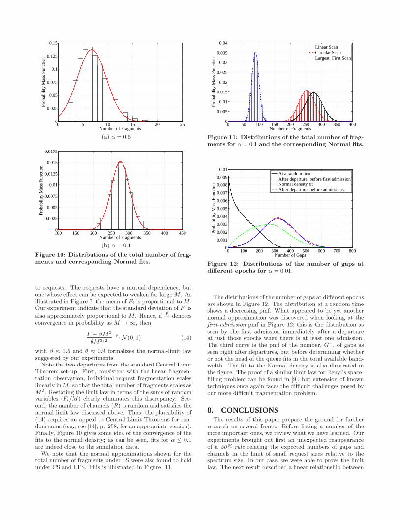
Interestingly, it was discovered in the experiments that anormal limit law also appears to hold for the total numberF of fragments as M → ∞ (see for example Figure 10).This is not surprising, since F is the sum over all requests insystem of the numbers Fi, 1 ≤ i ≤ R, of fragments allocated

0 5 10 15 20 250

0.025

0.05

0.075

0.1

0.125

0.15

Number of Fragments

Pro

babi

lity

Mas

s F

unct

ion

(a) α = 0.5

100 150 200 250 300 350 400 4500

0.0025

0.005

0.0075

0.01

0.0125

0.015

0.0175

Number of Fragments

Pro

babi

lity

Mas

s F

unct

ion

(b) α = 0.1

Figure 10: Distributions of the total number of frag-ments and corresponding Normal fits.

to requests. The requests have a mutual dependence, butone whose effect can be expected to weaken for large M . Asillustrated in Figure 7, the mean of Fi is proportional to M .Our experiment indicate that the standard deviation of Fi is

also approximately proportional to M . Hence, ifp→ denotes

convergence in probability as M → ∞, then

F − βM2

θM3/2

p→ N (0, 1) (14)

with β ≈ 1.5 and θ ≈ 0.9 formalizes the normal-limit lawsuggested by our experiments.

Note the two departures from the standard Central LimitTheorem set-up. First, consistent with the linear fragmen-tation observation, individual request fragmentation scaleslinearly inM , so that the total number of fragments scales asM2. Restating the limit law in terms of the sums of randomvariables (Fi/M) clearly eliminates this discrepancy. Sec-ond, the number of channels (R) is random and satisfies thenormal limit law discussed above. Thus, the plausibility of(14) requires an appeal to Central Limit Theorems for ran-dom sums (e.g., see [14], p. 258, for an appropriate version).Finally, Figure 10 gives some idea of the convergence of thefits to the normal density; as can be seen, fits for α ≤ 0.1are indeed close to the simulation data.

We note that the normal approximations shown for thetotal number of fragments under LS were also found to holdunder CS and LFS. This is illustrated in Figure 11.

0 50 100 150 200 250 300 350 4000

0.005

0.01

0.015

0.02

0.025

0.03

0.035

0.04

Number of Fragments

Pro

babi

lity

Mas

s F

unct

ion

Linear ScanCircular ScanLargest−First Scan

Figure 11: Distributions of the total number of frag-ments for α = 0.1 and the corresponding Normal fits.

0 100 200 300 400 500 600 700 8000

0.001

0.002

0.003

0.004

0.005

0.006

0.007

0.008

0.009

0.01

Number of Gaps

Pro

babi

lity

Mas

s F

unct

ion

At a random timeAfter departure, before first admissionNormal density fitAfter departure, before admissions

Figure 12: Distributions of the number of gaps atdifferent epochs for α = 0.01.

The distributions of the number of gaps at different epochsare shown in Figure 12. The distribution at a random timeshows a decreasing pmf. What appeared to be yet anothernormal approximation was discovered when looking at thefirst-admission pmf in Figure 12; this is the distribution asseen by the first admission immediately after a departureat just those epochs when there is at least one admission.The third curve is the pmf of the number, G−, of gaps asseen right after departures, but before determining whetheror not the head of the queue fits in the total available band-width. The fit to the Normal density is also illustrated inthe figure. The proof of a similar limit law for Renyi’s space-filling problem can be found in [9], but extension of knowntechniques once again faces the difficult challenges posed byour more difficult fragmentation problem.

8. CONCLUSIONSThe results of this paper prepare the ground for further

research on several fronts. Before listing a number of themore important ones, we review what we have learned. Ourexperiments brought out first an unexpected reappearanceof a 50% rule relating the expected numbers of gaps andchannels in the limit of small request sizes relative to thespectrum size. In our case, we were able to prove the limitlaw. The next result described a linear relationship between

the maximum request size, α, and the expected number offragments into which a request was divided at the time of al-location. Interestingly, the smaller α was taken, the greaterwas the resulting fragmentation of requests.

Our stability results established the beginning of a mathe-matical foundation of fragmentation processes. Particularly,we showed that for α > 1/2, the fragmentation process isHarris recurrent. For general α, we proved (with consider-able effort) that the total number of fragments is bounded inexpected value. We examined alternative algorithms for se-quencing through the available gaps and showed that usingthe LFS algorithm leads to significantly less fragmentationthan using the LS or CS algorithms. Finally, we exhibitedexperimentally a limiting, small-α behavior in which, withappropriate scaling, distributions tend to Normal.

A broad direction for further research extends the param-eters of our mathematical model. For instance, while Uni-form distributions are generally the assumption of choice infragmentation models, it would be interesting to see whatnew effects are created by other distributions of request size,e.g., by varying a in the generalized uniform distributions on[0, α], with densities xa/αa+1. The exponential residence-time assumption is likely to yield simplifications to analysis,but changes in behavior resulting from other distributionsare worth investigating. Moreover, instead of a system op-erating at capacity, in which there is always a request wait-ing, one could adopt an underlying, fully stochastic modelof demand, e.g., a Poisson arrival process, as found in [22].

More realistic, but in all likelihood significantly more diffi-cult models, would relax the independence assumptions. Aprime example appropriate for Dynamic Spectrum Accessapplications would be allowing residence times to depend onfragmentation, the greater the fragmentation of a request,the longer its residence time.

The results regarding the performance of the differentalgorithms imply that the algorithms’ design should alsobe considered carefully. Some examples of algorithms thatcome to mind will aim to better fit the fragments into theavailable gaps. A more challenging objective would be todevelop algorithms that take into account spectrum sensingcapabilities during the gap allocation process.

Finally, another broad and very important avenue of re-search that introduces more realistic models discretizes re-quest sizes and the bandwidth allocation process (as is beingdone while allocating OFDM subcarriers). As in other mod-els of fragmentation, the continuous limit represented in thispaper may conceal important effects, or, conversely, it mayintroduce effects not present in discrete models. We are ac-tively pursuing this avenue of research.

9. ACKNOWLEDGMENTSWe would like to thank Charles Bordenave for helpful dis-

cussions in relation with Theorem 4. This work was partiallysupported by NSF grant CNS-0916263 and CIAN NSF ERCunder grant EEC-0812072.

10. REFERENCES[1] I. F. Akyildiz, W.-Y. Lee, and K. R. Chowdhury. CRAHNs:

Cognitive radio ad hoc networks. Ad Hoc Networks,7(5):810–836, 2009.

[2] I. F. Akyildiz, W.-Y. Lee, M. C. Vuran, and S. Mohanty.NeXt generation/dynamic spectrum access/cognitive radiowireless networks: A survey. Comput. Netw.,50(13):2127–2159, Sep. 2006.

[3] S. Asmussen. Applied Probability and Queues. Springer,New York, NY, USA, 2nd edition, 1987.

[4] V. G. Bose, A. B. Shah, and M. Ismert. Software radios forwireless networking. In Proc. IEEE INFOCOM’98, Apr.1998.

[5] E. G. Coffman, Jr., A. A. Puhalskii, and M. I. Reiman.Storage limited queues in heavy traffic. Probab. Eng. andInfo. Sci., 5(4):499–522, 1991.

[6] E. G. Coffman, Jr. and M. I. Reiman. Diffusionapproximations for storage processes in computer systems.In Proc. ACM SIGMETRICS’83, 1983.

[7] DARPA XG WG, BBN Technologies. The XG architecturalframework version 1.0. 2003.

[8] DARPA XG WG, BBN Technologies. The XG vision RFCversion 2.0. 2003.

[9] A. Dvoretsky and H. Robbins. On the ‘parking’ problem.Publ. Math. Inst. Hung. Acad. Sci., 9:209–226, 1964.

[10] European Telecommunications Standards Institute. ETSIReconfigurable Radio. Documentation available athttp://www.etsi.org/WebSite/technologies/RRS.aspx.

[11] FCC. 03-222, Notice of Proposed Rulemaking, Oct. 2003.[12] FCC. 05-57, Report and Order, ET Docket No. 03-108,

Facilitating Opportunities for Flexible, Efficient, andReliable Spectrum Use Employing Cognitive RadioTechnologies, Mar. 2005.

[13] FCC. 08-260, Second Report and Order, ET Docket No.04-186, Unlicensed Operation in the TV Broadcast Bands,Nov. 2008.

[14] W. Feller. An Introduction to Probability Theory and ItsApplications, Volume II. John Wiley & Sons, New York,NY, USA, 2nd edition, 1966.

[15] S. Geirhofer, L. Tong, and B. Sadler. Interference-awareOFDMA resource allocation: A predictive approach. InProc. IEEE MILCOM’08, Nov. 2008.

[16] A. Ghasemi and E. Sousa. Spectrum sensing in cognitiveradio networks: Requirements, challenges and designtrade-offs. IEEE Commun., 46(4):32–39, Apr. 2008.

[17] B. Hajek. Hitting-time and occupation-time bounds impliedby drift analysis with applications. Adv. Appl. Probab.,14(3):502–525, 1982.

[18] W. Hou, L. Yang, L. Zhang, X. Shan, and H. Zheng.Understanding cross-band interference in unsynchronizedspectrum access. In Proc. ACM CoRoNet’09, 2009.

[19] IEEE 802.22, Working Group on Wireless Regional AreaNetworks (“WRANs”). Documentation available athttp://ieee802.org/22/.

[20] IEEE Standards Coordinating Committee 41 (DynamicSpectrum Access Networks). Documentation available athttp://www.scc41.org/.

[21] J. Jia, Q. Zhang, and X. Shen. HC-MAC: Ahardware-constrained cognitive MAC for efficient spectrummanagement. IEEE J. Sel. Areas Commun., 26(1):106–117,Jan. 2008.

[22] C. Kipnis and P. Robert. A dynamic storage process.Stochastic processes and their applications, 34(1):155–169,1990.

[23] D. E. Knuth. The Art of Computer Programming, Vol. 1 -Fundamental Algorithms. Addison Wesley LongmanPublishing Co., Redwood City, CA, USA, 3rd edition, 1997.

[24] W. Krenik, A. M. Wyglinski, and L. E. Doyle (eds.).Cognitive radios for dynamic speactrm access. SpecialIssue, IEEE Commun., 45(5):64–65, May 2007.

[25] H. Mahmoud, T. Yucek, and H. Arslan. OFDM forcognitive radio: Merits and challenges. IEEE WirelessCommun., 16(2):6–15, Apr. 2009.

[26] P. Mahonen and M. Zorzi (eds.). Cognitive wirelessnetworks. Special Issue, IEEE Wireless Commun.,14(4):4–5, Aug. 2007.

[27] J. Mitola III. Cognitive radio for flexible mobile multimediacommunications. In Proc. IEEE MoMuC’99, Nov. 1999.

[28] J. Mitola III. Cognitive Radio: An Integrated Agent

Architecture for Software Defined Radio. PhD thesis,Doctor of Technology, Royal Inst. Technol. (KTH),Stockholm, Sweden, 2000.

[29] J. D. Poston and W. D. Horne. Discontiguous OFDMconsiderations for dynamic spectrum access in idle TVchannels. In Proc. IEEE DySPAN’05, Nov. 2005.

[30] R. Rajbanshi, A. M. Wyglinski, and G. J. Minden.OFDM-based cognitive radios for dynamic spectrum accessnetworks. In V. K. Bhargava and E. Hossain, editors,Cognitive Wireless Communication Networks, pages165–188. Springer-Verlag, 2007.

[31] A. Shukla, B. Willamson, J. Burns, E. Burbidge, A. Taylor,and D. Robinson. A study for the provision of aggregationof frequency to provide wider bandwidth services. Technicalreport, QinetiQ, Aug. 2006.

[32] T. A. Weiss and F. K. Jondral. Spectrum pooling: Aninnovative strategy for the enhancement of spectrumefficiency. IEEE Commun., 42(3):S8–14, Mar. 2004.

[33] Y. Yuan, P. Bahl, R. Chandra, T. Moscibroda, and Y. Wu.Allocating dynamic time-spectrum blocks in cognitive radionetworks. In Proc. ACM MobiHoc’07, 2007.

APPENDIX

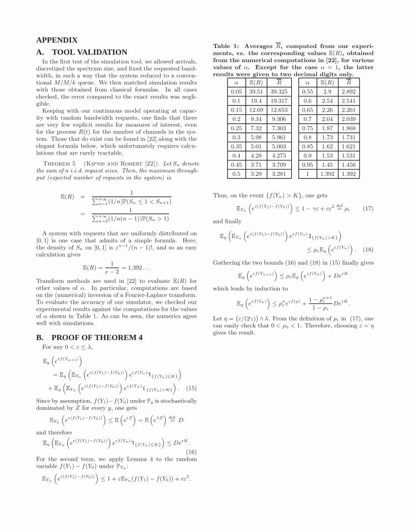
A. TOOL VALIDATIONIn the first test of the simulation tool, we allowed arrivals,

discretized the spectrum size, and fixed the requested band-width, in such a way that the system reduced to a conven-tional M/M/k queue. We then matched simulation resultswith those obtained from classical formulas. In all caseschecked, the error compared to the exact results was negli-gible.

Keeping with our continuous model operating at capac-ity with random bandwidth requests, one finds that thereare very few explicit results for measures of interest, evenfor the process R(t) for the number of channels in the sys-tem. Those that do exist can be found in [22] along with theelegant formula below, which unfortunately requires calcu-lations that are rarely tractable.

Theorem 5 (Kipnis and Robert [22]). Let Sn denotethe sum of n i.i.d. request sizes. Then, the maximum through-put (expected number of requests in the system) is

E(R) =1

∑+∞n=1(1/n)P(Sn ≤ 1 < Sn+1)

=1

∑+∞n=2(1/n(n− 1))P(Sn > 1)

A system with requests that are uniformly distributed on[0, 1] is one case that admits of a simple formula. Here,the density of Sn on [0, 1] is zn−1/(n − 1)!, and so an easycalculation gives

E(R) =1

e− 2= 1.392 . . .

Transform methods are used in [22] to evaluate E(R) forother values of α. In particular, computations are basedon the (numerical) inversion of a Fourier-Laplace transform.To evaluate the accuracy of our simulator, we checked ourexperimental results against the computations for the valuesof α shown in Table 1. As can be seen, the numerics agreewell with simulations.

B. PROOF OF THEOREM 4For any 0 < ε ≤ λ,

Ey

(

eεf(Yn+1))

= Ey

(

EYn

(

eε(f(Y1)−f(Y0)))

eεf(Yn)1{f(Yn)≤K}

)

+ Ey

(

EYn

(

eε(f(Y1)−f(Y0)))

eεf(Yn)1{f(Yn)>K}

)

. (15)

Since by assumption, f(Y1)−f(Y0) under Py is stochasticallydominated by Z for every y, one gets

EYn

(

eε(f(Y1)−f(Y0)))

≤ E

(

eεZ)

= E

(

eλZ)

def.= D

and therefore

Ey

(

EYn

(

eε(f(Y1)−f(Y0)))

eεf(Yn)1{f(Yn)≤K}

)

≤ DeεK .

(16)For the second term, we apply Lemma 4 to the randomvariable f(Y1) − f(Y0) under PYn

:

EYn

(

eε(f(Y1)−f(Y0)))

≤ 1 + εEYn(f(Y1) − f(Y0)) + cε2.

Table 1: Averages R, computed from our experi-ments, vs. the corresponding values E(R), obtainedfrom the numerical computations in [22], for variousvalues of α. Except for the case α = 1, the latterresults were given to two decimal digits only.

α E(R) R α E(R) R

0.05 39.51 39.325 0.55 2.9 2.892

0.1 19.4 19.317 0.6 2.54 2.541

0.15 12.69 12.653 0.65 2.26 2.261

0.2 9.34 9.306 0.7 2.04 2.039

0.25 7.32 7.303 0.75 1.87 1.868

0.3 5.98 5.961 0.8 1.73 1.731

0.35 5.01 5.003 0.85 1.62 1.621

0.4 4.28 4.275 0.9 1.53 1.531

0.45 3.71 3.709 0.95 1.45 1.456

0.5 3.29 3.281 1 1.392 1.392

Thus, on the event {f(Yn) > K}, one gets

EYn

(

eε(f(Y1)−f(Y0)))

≤ 1 − γε+ cε2def= ρε (17)

and finally

Ey

(

EYn

(

eε(f(Y1)−f(Y0)))

eεf(Yn)1{f(Yn)>K}

)

≤ ρεEy

(

eεf(Yn))

. (18)

Gathering the two bounds (16) and (18) in (15) finally gives

Ey

(

eεf(Yn+1))

≤ ρεEy

(

eεf(Yn))

+DeεK

which leads by induction to

Ey

(

eεf(Yn))

≤ ρnε e

εf(y) +1 − ρn+1

ε

1 − ρεDeεK .

Let η =(

ε/(2γ))

∧λ. From the definition of ρε in (17), onecan easily check that 0 < ρη < 1. Therefore, choosing ε = ηgives the result.