CHAOS IN WATER BODY EUTROPHICATION Sandra Regina F.A. da Silva Instituto Militar de Engenharia Departamento de Engenharia Mecânica e de Materiais 22.290.270 − Rio de Janeiro − RJ Marcelo Amorim Savi Universidade Federal do Rio de Janeiro COPPE - Departamento de Engenharia Mecânica 21.945.970 − Rio de Janeiro − RJ E-Mail: savi@ufrj.br Mariana Erthal Rocha Universidade Santa Úrsula Instituto de Ciências Biológicas e Ambientais 22.231.040 − Rio de Janeiro – RJ Abstract. The word eutrophication comes from greek and means “well-nourished”. This is employed to denote the process of nutrient addition in water bodies and its effects. The present contribution analyzes the dynamics of water body eutrophication from a mathematical model with five variables: nutrients, phytoplankton, zooplankton and two different kinds of fishes. Basically, a nonlinear dynamical system, discrete in space and continuous in time is proposed. Dynamical system is based on species competition / population evolution and its elaboration involves the definition of a food chain that is based on complex relations among animals and plants. Eutrophication dynamics is analyzed showing different kinds of response including chaos. The model is capable to capture the general behavior related to eutrophication process in a qualitative point of view. Key-words: Eutrophication, water, nonlinear dynamics, chaos, ecological systems.

1. Introduction

The word eutrophication comes from greek and means “well-nourished”. This is employed to denote the process of nutrient addition in water bodies and its effects. Therefore, it is a phenomenon that is understood as the enrichment of biological systems by nutrient elements, organic and inorganic matter, notably phosphorus and nitrogen. The natural process of eutrophication can be culturally accelerated by human interference. External sources of nutrients includes municipal and industrial wastes, agricultural and forest runoff, urban runoff and atmospheric fallout (Thomann & Mueller, 1987).

Cultural process of eutrophication is perhaps one of the main problems related to the water quality. This process may present drastic consequences to the environmental system breaking its ecological equilibrium. Therefore, the analysis of the impact of human activities on the eutrophication process and its control is of special interest for the environment.

The elevated level of nutrients promotes the growth of aquatic plants, which can be classified into two categories: those that move freely with the water (planktonic) and those that remain fixed. The first category includes the phytoplankton that is related to different kinds of algae, while the second includes rooted aquatic plants of various sizes (benthic algae). In all cases, plants obtain the primary energy source from sunlight through the photosynthesis process.

Similar to aquatic plants, animal population in a water body may be classified into two different categories: zooplankton, which can move freely with the water and fishes. Zooplankton is the primary consumer of phytoplankton population and fishes consume either phytoplankton or zooplankton.

The excessive discharge of nutrients in water bodies tends to produce phytoplankton blooms and growth of aquatic weeds. This is a consequence of conversion of inorganic nutrients into organic matter from photosynthesis process. Algae bloom promotes nutrients and oxygen reduction that causes phytoplankton, zooplankton and fishes death.

The modeling of biological phenomena by mathematical models has increasing importance in recent years. These models may describe time evolution and spatial distribution and may explain some important characteristics of these systems. The mathematical analysis is exploiting the possibility that many biological phenomena or medical problems may have their roots in some underlying dynamical effect: the so-called dynamical diseases (Holton & May, 1993). Alligood et al. (1997) say that “of course, the idea of a real experiment being governed by a set of equations is a fiction. A set of differential equations, or a map, may model the process closely enough to achieve useful goals”. Moreover, Segel (1984) presents the following argument (Rafikov, 2002): “ ‘Art is the lie that helps us see the truth’ said Picasso, and the same can be said of modeling. On seeing a Picasso sculpture of a goat, we are amazed that his caricature seems more goatlike than the real animal, and we may gain a much stronger feeling for ‘goatness’. Similarly, a good mathematical model – though distorted and hence ‘wrong’, like any simplified representation of reality – will reveal some essential components of a complex phenomenon”.

Recently, many authors are devoted to propose a theoretical framework to deal with ecological systems (Salthe, 2002; Reynolds, 2002; Odum, 2002; Jørgensen, 2002). Marques & Jørgensen (2002) say that “biology and ecology are more complex than physics, an it will, therefore, be much more difficult to develop an applicable, predictive ecological

theory… But most biologists and ecologists probably feel inwards the need for a more general and integrative theory that may help in explaining their observations and experimental results.”

Literature presents different models to describe ecological systems. In mathematical point of view, they can be classified into three different classes: maps, which are discrete in space and time; ordinary differential equations (ODEs), which is discrete in space and continuous in time; and partial differential equations (PDEs), which are continuous in space and time.

Population evolution models are usually based on prey-predator systems or species competition. These models could consider different variables, describing their interactions. Perhaps, the first model for population evolution is the linear model due to Malthus. A nonlinear alternative is based on the logistic equation (May, 1976). Lotka-Volterra model presents the first description of predator-prey model (Lotka, 1925; Volterra, 1926).

The analysis of aquatic populations is done with all of the cited approaches. Rinaldi & Solidoro (1998) consider maps to describe plankton-fish interaction. EDOs are also considered in the analysis of plankton and aquatic populations (Doveri et al., 1993; Solé, 1999; Vandermeer et al., 2001; Edwards & Bees, 2001; Scheren, 2000; Lecture & Mäler, 2000). On the other hand, PDEs are employed to describe either the time evolution or the spatial distribution of aquatic population (Malchow et al., 2000; Mordasova, 1999; Sorokin et al., 1998; Gilbert & Giavarini, 2000).

Alternative approaches are also used in order to describe eutrophication process. Triantafyllou et al. (2000) describes benthic communities analyzing physico-chemical alterations related to functional groups. Menéndez & Comin (2000) considers a statistical analysis of algae proliferation during spring and summer; Al-Homaida & Arif (1998) develop an experimental analysis of algae bloom at Al-Kharj, Saudi Arabia. Aoki (1997) treats maturation of eutrophic lakes using tolls of information theory. In recent years, chaos is of concerned associating this kind of response with different biological behaviors (Medvinsky et al., 2002; Medvinsky et al., 2001a; Medvinsky et al., 2001b; Tikhonov et al., 2001; Edwards & Bees, 2001; Malchow et al., 2000; Péntek et al., 1999; Doveri et al., 1993; Rinaldi & Solidoro, 1998; Jørgensen, 1995; Seip et al., 1994).

The present contribution analyzes the dynamics of water body eutrophication from a mathematical model. Basically, a nonlinear dynamical system, discrete in space and continuous in time is proposed (EDOs). Dynamical system is based on species competition (populational evolution) and its elaboration involves the definition of a food chain that is based on complex relations among animals and plants. The proposed model considers five variables: nutrients, phytoplankton, zooplankton and two different kinds of fishes. Eutrophication dynamics is analyzed showing different kinds of response including chaos. The model is capable to capture the general behavior related to eutrophication process. 2 – Mathematical Model

In order to establish a model to describe the dynamics of water body eutrophication, a discrete water volume is

considered. Moreover, a food chain with five variables is analyzed: nutrients, N, phytoplankton, F, zooplankton, Z, and two different kinds of fishes (phytoplanktivorous, PF, and zooplanktivorous, PZ). Figure 1 presents a schematic picture that establishes the food chain with these variables. Nutrients are consumed by phytoplankton, which may be consumed by zooplankton and phytoplanktivorous fishes. On the other hand, zooplanktivorous fishes may consume zooplankton. From these five variables, a conceptual model is proposed as suggested by Figure 2.

Figure 1 – Schematic picture of the food chain.

Figure 2 – Conceptual model. Basically, nutrient has an inflow defined by α(t) and an outflow with a constant rate, δ. Moreover, this nutrient is

consumed by phytoplankton with a rate, β. Phytoplankton grows as a consequence of an inflow, ε, and also to the nutrient availability. The term, γβFP defines

this interaction. Parameter γ is related to the solar radiation and other photosynthesis conditions. This population may decrease as a consequence of outflow, λ, or by the zooplankton consumption, η. Zooplankton has an inflow µ and outflow ψ. The term νηFZ establishes the interaction with phytoplankton. Parameter ν defines consumption conditions and c establishes quadratic interactions between phytoplankton and nutrients, while κ, the same interaction between and phytoplankton and zooplankton. Zooplankton competition with the own specie is described by the term . 2Zϕ

Phytoplanktivorous fishes have an inflow, ρ. The interaction between phytoplankton and fish is defined by the term . The term, describes variable quadratic interactions, establishing that phytoplankton has importance

with respect to water conditions as oxygen. Moreover, there is an outflow θ, and also, a competition with the own specie, .

21 FPFφτ

3τ

22 FPFτ

2FP

With respect to the zooplanktivorous fish, its equation has an inflow ς, and an interaction with zooplankton defined by the term ZPZζυ1 . Moreover, there is quadratic interaction related to the phytoplankton, . Also, there is an

outflow, σ, and the specie own competition, described by the term, .

22 FPZυ

23 ZPυ

Therefore, the following mathematical model is proposed:

(1)

ZZZZZ

FFFFF

ZZ

F

PPFPZPP

PPFPFPP

ZFPZPcZFZ

FFPcZFZkFPFF

PkFPFtP

συυζυς

θττφτρ

ψηζνηµ

λφηγβε

δβα

−−−+=

−−−+=

−−−++=

−−+−++=

−+−=

23

221

23

221

221 )1(

)1()1(

)1()(

&

&

&

&

&

Notice that for a specific volume, parameters are constants related to other variables like oxygen, luminosity and

temperature. Moreover, the term α(t) represents nutrients inflow, understood as a driving force: )sin()( 00 tFt ωαα += . The term α0 may represent any inflow described by linear piecewise functions. The sinusoidal

term is related to oscillations around α0. Non-dimensional variables are considered and time scale may be related to days, months or years.

Numerical simulations consider fourth order Runge-Kuta method in order to perform time integration of equations.

3. Parameter Analysis In order to analyze system parameters, a simple procedure is proposed. Basically, a single interaction is considered,

vanishing all other terms in governing equations. This procedure is similar to a laboratory experiment, where two system variables are isolated. With these assumptions, it is possible to vary parameter values in order to induce variables to reach experimental values. In this article, reference values are related to Rodrigo de Freitas Lake, Rio de Janeiro – Brazil (Andreata, 2001).

As an example, consider the interaction between nutrients and phytoplankton. Hence, parameters β, γ, k, and λ are analyzed, vanishing the others. At first, parameter β is considered. Figure 3 presents numerical simulation related to the

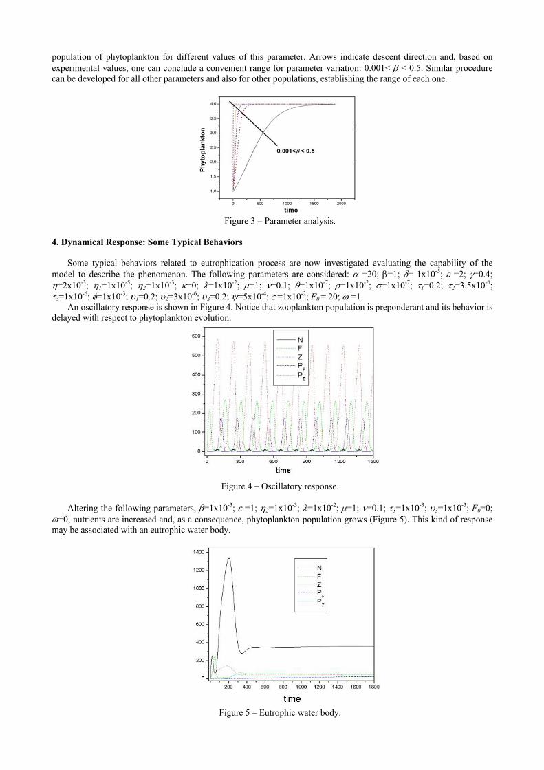
population of phytoplankton for different values of this parameter. Arrows indicate descent direction and, based on experimental values, one can conclude a convenient range for parameter variation: 0.001< β < 0.5. Similar procedure can be developed for all other parameters and also for other populations, establishing the range of each one.

Phyt

opla

nkto

n time

Figure 3 – Parameter analysis.

4. Dynamical Response: Some Typical Behaviors Some typical behaviors related to eutrophication process are now investigated evaluating the capability of the

model to describe the phenomenon. The following parameters are considered: α =20; β=1; δ= 1x10-5; ε =2; γ=0.4; η=2x10-3; η1=1x10-5; η2=1x10-3; κ=0; λ=1x10-2; µ=1; ν=0.1; θ=1x10-7; ρ=1x10-2; σ=1x10-7; τ1=0.2; τ2=3.5x10-6; τ3=1x10-6; φ=1x10-3; υ1=0.2; υ2=3x10-6; υ3=0.2; ψ=5x10-4; ς =1x10-2; F0 = 20; ω =1.

An oscillatory response is shown in Figure 4. Notice that zooplankton population is preponderant and its behavior is delayed with respect to phytoplankton evolution.

Figure 4 – Oscillatory response.

Altering the following parameters, β=1x10-3; ε =1; η2=1x10-3; λ=1x10-2; µ=1; ν=0.1; τ3=1x10-3; υ3=1x10-3; F0=0;

ω=0, nutrients are increased and, as a consequence, phytoplankton population grows (Figure 5). This kind of response may be associated with an eutrophic water body.

Figure 5 – Eutrophic water body.

Altering parameters β =1x10-2; F0 = 20; ω = 1, keeping the others as before, the system presents an oscillatory

response again (Figure 6). Nevertheless, there is a dissipation characteristic. Notice that phytoplanktivorous fishes tend to decrease indicating an excessive population of phytoplankton.

Figure 6 – Oscillatory response with dissipation.

Varying parameters β =1.5; ε = 2 and γ = 0.6 (Figure 7a), fish populations (PF and PZ), has a significantly decrease.

On the other hand, assuming γ = 0.7 (Figure 7b), phytoplankton population dominates the response and fish populations tends to vanish. This second behavior is related to algae bloom.

Figure 7 – Algae bloom.

5. Dynamics Investigation This section is concerned with a dynamics investigation of the proposed model. This investigation provides a

picture of all possibilities related to the eutrophication phenomenon, considering different kinds of behaviors. This analyzes employs some nonlinear tools related to the literature of nonlinear dynamics and chaos. Since the proposed model is a six-dimensional system, the visualization of phase space becomes difficult, and it is necessary to consider projections in subspaces. One of this subspaces considers fish populations, P = PF + PZ, even though this is not a state variable.

In order to start the analysis, bifurcation diagrams are considered. This diagram represents the stroboscopically sampled variable values under the slow quasi-static increase of a system parameter. Basically, the analysis of parameter γ, in the range (0, 1), is of concerned. When γ = 0, there is no luminosity, and when γ = 1, it assumes a maximum value. The following parameters are considered: α =20; β =1x10-5; δ = 1x10-2; ε = 2; η =2x10-4; η1 =1x10-5; η2=1x10-6; κ=1x10-4; λ=1x10-3; µ=1; ν=0.02; θ=1x10-7; ρ =1x10-2; σ =1x10-7; τ1=0.2; τ2=3.5x10-6; τ3=1x10-3; φ =1x10-3; υ1=0.2; υ2=3x10-6; υ3=1x10-3; ψ=1x10-3; ς=1x10-3. Figure 8 presents different variables of the system under the variation of parameter γ. Notice regions related to different number of points, indicating periodic responses, and also cloud of points, associated with chaos.

Nut

rient

s

Phyt

opla

nkto

n

Figure 8 – Bifurcation diagrams under the variation of parameter γ. It is convenient to enlarge some regions of bifurcation diagrams in order to obtain a better comprehension of the

system dynamics. Figure 9 and 10 presents these enlargements for different variables. Figure 9 shows the range 0.31 ≤ γ ≤ 0.37, while Figure 10 shows a periodic window, inside a chaotic region.

Figure 9 – Enlargement in the range 0.31 ≤ γ ≤ 0.37.

Figure 10 – Enlargement of periodic window.

Bifurcation diagrams provide a global picture of the system’s dynamics, indicating qualitative changes in the system response. The forthcoming analysis considers different parameter values, showing the kind of response for each one. The visualization of the system behavior is done considering subspaces of Poincaré section of the system, which is obtained by sampling state variables of the system at a rate equal to the forcing period. At first, γ = 0.28 is assumed. This value is related to a period-1 response, as could be seen in Poincaré sections of Figure 11.

Figure 11 – Period-1 response, γ = 0.28. After several bifurcations, for γ = 0.4, the system presents a chaotic response (Figure 12). This conclusion is

assured assessing Lyapunov exponents that evaluate the sensitive dependence to initial conditions estimating the exponential divergence of nearby orbits. These exponents have been used as the most useful dynamical diagnostic tool for chaotic system analysis. The signs of Lyapunov exponents provide a qualitative picture of the system’s dynamics and any system containing at least one positive exponent presents chaotic behavior. The algorithm due to Wolf et al. (1985) is employed showing one positive value.

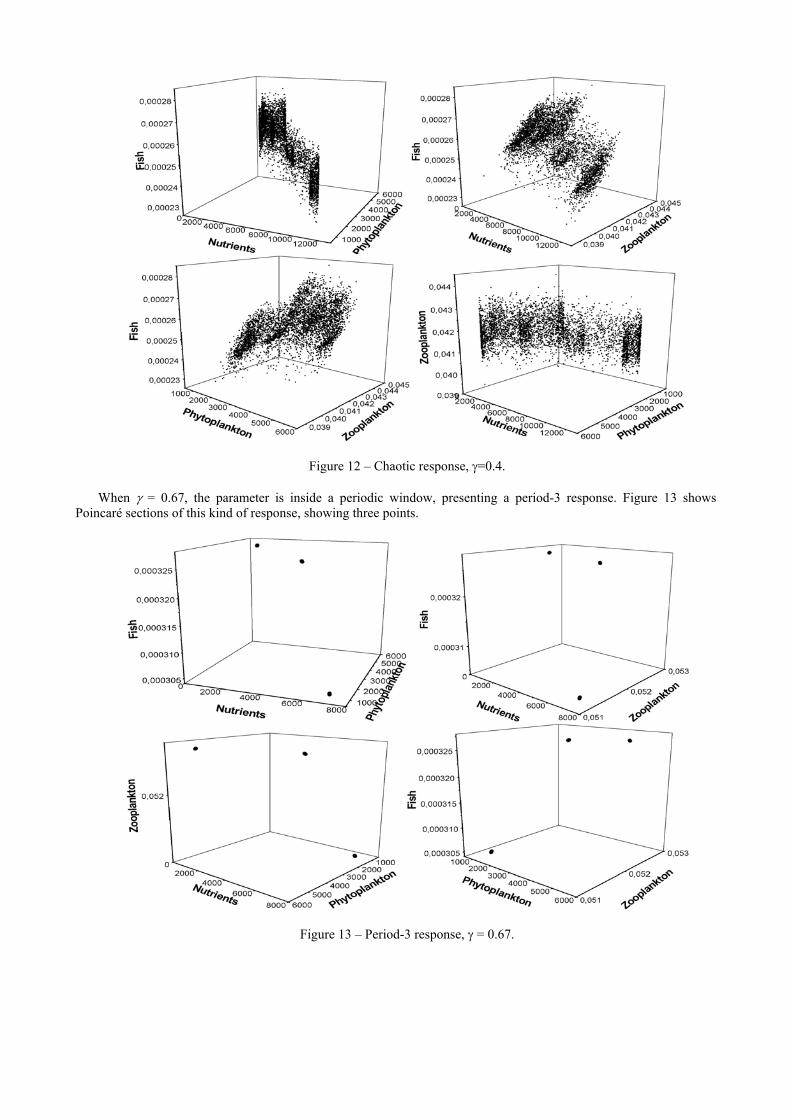
Figure 12 – Chaotic response, γ=0.4. When γ = 0.67, the parameter is inside a periodic window, presenting a period-3 response. Figure 13 shows

Poincaré sections of this kind of response, showing three points.

Figure 13 – Period-3 response, γ = 0.67.

6. Conclusions This article considers a mathematical model to describe the dynamics of water body eutrophication. Basically, the

proposed model is a nonlinear system, discrete in space and continuous in time, employing five variables: nutrients, phytoplankton, zooplankton, phytoplanktivorous fish and zooplanktivorous fish. A procedure to estimate system parameters is proposed. Numerical simulations are carried out showing that the model is capable to capture the general behavior related to eutrophication process. A more detailed investigation of the system behavior shows that its dynamical response is very rich. Periodic and chaotic responses are possible. The variety of responses obtained by the mathematical model encourages its use to describe ecological systems and, at least as a caricature of the reality, it could furnish useful information. The authors agree that this article contributes to the use of mathematical models to describe dynamics of water body eutrophication. Nevertheless, other studies must be carried out in order to calibrate the proposed model.

7. Acknowledgements

The authors acknowledge the support of the Brazilian Agencies CNPq and CAPES.

8. References Alligood, K. T., Sauer, T. D. & Yorke, J. A., 1997. “Chaos: An Introduction to Dynamical Systems”, Springer-Verlag. Andreata, J.V., 2001. “Lagoa Rodrigo de Freitas: Síntese Histórica e Ecológica”, Universidade Santa Úrsula. Aoki, I., 1997. “Comparative Study of Flow-indices in Lake-ecosystems and the Implication for Maturation Process”,

Ecological Modeling, v. 95, p.165-169. Al-Homaida, A.A. & Arif, I.A., 1998. “Ecology and Bloom Forming Algae of a Semi-permanent Rain-fed Pool at Al-

Kharj, Saudi Arabia”, Journal of Arid Environments, v.38, p.15-25. Doveri, F., Scheffer, M., Rinaldi, S., Muratori, S. & Kuznetsov, Y., 1993. “Seasonality and Chaos in a Plankton Fish

Model”, Theoretical Population Biology, v.43, n.2, p.159-183. Edwards, A.M. & Bees, M.A., 2001. “Generic Dynamics of a Simple Plankton Population Model with a Non-integer

Exponent of Closure”, Chaos, Solitons & Fractals, v.12, n.2, p.289-300. Gilbert, O. & Giavarini, V., 2000. “The Lichen Vegetation of Lake Margins in Britain”, Lichenologist, v.32, p. 365-386. Holton, D. & May, R.M., 1993. “The Chaos of Disease Response and Competition”, in The Nature of Chaos Ed. Tom

Mullin, Oxford. Jørgensen, S.E., 1995. “The Growth Rate of Zooplankton at the Edge of Chaos: Ecological Models”, Journal of

Theoretical Biology, v.175, p.13-21. Jørgensen, S.E., 2002. “Explanation of Ecological Rules and Observation by Application of Ecosystem Theory and

Ecological Models”, Ecological Modelling, v.158, n.3, p.241-248. Lecture, J.S. & Mäler, K., 2000. “Development, Ecological Resourcews and their Management: A Study of Complex

Dynamic Systems”, European Economic Review, v.44, p.645-665. Lotka, A.J., 1925. “Elements of Physical Biology”, William and Wilkins. Malchow, H., Radtke, B., Kallache, M., Medvinsky, A.B., Tikhonov, D.A., & Petrovskii, S.V., 2000. “Spatio-temporal

Pattern Formation in Coupled Models of Plankton Dynamics and Fish School Motion”, Nonlinear Analysis: Real World Applications, v.1, n.1, p.53-67.

Marques, J.C. & Jørgensen, S.E., 2002. “Three Selected Ecological Observations Interpreted in Terms of a Thermodynamic Hypothesis: Contribution to a General Theoretical Framework”, Ecological Modelling, v.158, n.3, p.213-221.

May, R.M., 1976. “Simple Mathematical Models With Very Complicated Dynamics”, Nature, v.261, p.459-467. Medvinsky, A.B., Tikhonova, I.A., Petrovskii, S.V., Malchow, H. & Venturino, E., 2002. “Chaos and Order in Plankton

Dynamics: Complex Behavior of a Simple Model”, Zhurnal Obshchei Biologii, v.63, n.2, p.149-158. Medvinsky, A.B., Petrovskii, S.V., Tikhonova, I.A., Venturino, E. & Malchow, H., 2001a. “Chaos and Regular

Dynamics in Model Multi-habitat Plankton-Fish Communities”, Journal of Biosciences, v.26, n.1, p. 109-120. Medvinsky, A.B., Petrovskii, S.V., Tikhonov, D.A., Tikhonova, I.A., Ivanitsky, G.R. & Malchow, H., 2001b.

“Biological Factors Underlying Regularity and Chaos in Aquatic Ecosystems: Simple Models of Complex Dynamics”, Journal of Biosciences, v.26, n.1, p.77-108.

Menéndez, M. & Comin, F.A., 2000. “Spring and Summer Proliferation of Floating Macroalgae in a Mediterranean Coastal Lagoon (Tancada Lagoon, Ebro Delta, NE Spain)”, Estuarine, Coastal and Shelf Science, v.51, p.215-226.

Mordasova, N.V., 1999. “Chlorophyll in the White Sea”, ICES - Journal of Marine Science, v.56, p.215-218. Odum, H.T., 2002. “Explanations of Ecological Relationships with Energy Systems Concepts”, Ecological Modelling,

v.158, n.3, p.201-211. Péntek, Á., Károlyi, G., Scheuring, I., Tél, T., Toroczkai, Z., Kadtke, J. & Grebogi, C., 1999. “Fractality, Chaos, and

Reactions in Imperfectly Mixed Open Hydrodynamical Flows”, Physica A, v.274, n.1-2, p.120-131. Rafikov, M., 2002. “Aplicação da Teoria de Controle Ótimo em Dinâmica Populacional”, I Congresso Temático de

Dinâmica, Controle e Aplicações, 29 julho – 01 agosto, São José do Rio Preto, DINCON. Reynolds, C.S., 2002. “Ecological Pattern and Ecosystem Theory”, Ecological Modelling, v.158, n.3, p.181-200.

Rinaldi, S. & Solidoro, C., 1998. “Chaos and Peak-to-Peak Dynamics in a Plankton-Fish Model”, Theoretical Population Biology, v.54, p.62-77.

Salthe, S.N., 2002. “An Exercise in the Natural Philosophy of Ecology”, Ecological Modelling, v.158, n.3, p.167-179. Sorokin, Y.I., Sorokin, P.Y. & Ravagnan, G., 1999. “Analysis of Lagoonal Ecosystems in the Po River Delta

Associated whith Intensive Aquaculture”, Estuarine, Coastal and Shelf Science, v.48, p.325-341. Segel, L.A., 1984. “Modeling Dynamic Phenomena in Molecular and Cellular Biology”, Cambridge Univ. Press. Seip, K.L., Sneek, M. & Snipen, L.-G., 1994. “How Far Do Physical Factors Determine Phytoplankton Biomass in

Lakes?”, Chemometrics and Intelligent Laboratory Systems, v.23, p.247-258. Sheren, P.A.G.M., Zanting, H.A., & Lemmens, A.M.C., 2000. “Estimation of Water Pollution Sources in Lake Victoria,

East Africa: Application and Elaboration of the Rapid Assessment Methodology”, Journal of Environmental Management, International Council for the Exploration of the Sea, v.58, p. 235-248.

Solé, R.V., Gamarra, J.P., Ginovart, M. & López, D., 1999. “Controlling Chaos in Ecology: From Deterministic to Individual-based Models”, Bulletin of Mathematical Biology, v. 61, p. 1187-1207.

Thomann, R.V. & Mueller, J.A., 1987. “Principles of Surface Water Quality Modeling and Control”, Harper Collins. Tikhonov, D.A., Enderlein, J., Malchow, H. & Medvinsky, A.B., 2001. “Chaos and Fractals in Fish School Motion”,

Chaos, Solitons & Fractals, v.12, n.2, p.277-288. Triantafyllou, G., Petihakis, C., Dounas, C., Koutsoubas, D., Arvanitidis, C. & Eleftheriou, A., 2000. “Temporal

Variations in Benthic Communities and their Response to Physicochemical Forcing: A Numerical Approach”, ICES Journal of Marine Science, v. 57, p. 1507-1516.

Vandermeer, J., Stone, L. & Blasius, B., 2001. “Categories of Chaos and Fractal Basin Boundaries in Forced Predator-Prey Models”, Chaos, Solitons and Fractal, v. 12, p. 265-276.

Volterra, V., 1926. “Fluctuations in the Abundance of a Species Considered Mathematically”, Nature, v. 118, p. 558-560.

Wolf, A., Swift, J.B., Swinney, H.L. & Vastano, J.A., 1985. “Determining Lyapunov Expoents from a Times Series”, Physica 16D, p. 285-317.