Embed Size (px)
Citation preview
November 9, 2020 1:40 ws-rv9x6 Book Title main page 1
Chapter 1
Bayesian Neural Networks
Tom Charnock1, Laurence Perreault-Levasseur2, Francois Lanusse3
1Sorbonne Universite, CNRS, UMR 7095, Institut d’Astrophysique deParis,
98 bis bd Arago, 75014 Paris, France,
2Department of Physics, Univesite de Montreal, Montreal, Canada,Mila - Quebec Artificial Intelligence Institute, Montreal, Canada, andCenter for Computational Astrophysics, Flatiron Institute, New York,
USA
3AIM, CEA, CNRS, Universite Paris-Saclay, Universite Paris Diderot,Sorbonne Paris Cite, F-91191 Gif-sur-Yvette, France
In recent times, neural networks have become a powerful tool for theanalysis of complex and abstract data models. However, their intro-duction intrinsically increases our uncertainty about which features ofthe analysis are model-related and which are due to the neural network.This means that predictions by neural networks have biases which can-not be trivially distinguished from being due to the true nature of thecreation and observation of data or not. In order to attempt to addresssuch issues we discuss Bayesian neural networks: neural networks wherethe uncertainty due to the network can be characterised. In particular,we outline the Bayesian statistical framework which allows us to cat-egorise uncertainty in terms of the ingrained randomness of observingcertain data and the uncertainty from our lack of knowledge about howprocesses that are observed can occur. In presenting such techniques weshow how uncertainties which arise in the predictions made by neuralnetworks can be characterised in principle. We provide descriptions ofthe two favoured methods for analysing such uncertainties. We will alsodescribe how both of these methods have substantial pitfalls when put
1
arX
iv:2
006.
0149
0v2
[st
at.M
L]
6 N
ov 2
020
November 9, 2020 1:40 ws-rv9x6 Book Title main page 2
2 Charnock, Perreault-Levasseur, Lanusse
into practice, highlighting the need for other statistical techniques totruly be able to do inference when using neural networks.
Contents
1. Introduction . . . . . . . . . . . . . . . . . . . . . . . . . . . . . . . . . . . . . 21.1. The need for statistical modelling . . . . . . . . . . . . . . . . . . . . . . 2
1.2. Aleatoric and epistemic uncertainty . . . . . . . . . . . . . . . . . . . . . 3
2. Bayesian neural networks . . . . . . . . . . . . . . . . . . . . . . . . . . . . . . 52.1. Bayesian statistics . . . . . . . . . . . . . . . . . . . . . . . . . . . . . . . 5
2.2. Neural networks formulated as statistical models . . . . . . . . . . . . . 11
3. Practical implementations . . . . . . . . . . . . . . . . . . . . . . . . . . . . . 163.1. Numerically approximate inference:
Monte Carlo methods . . . . . . . . . . . . . . . . . . . . . . . . . . . . . 16
3.2. Variational Inference . . . . . . . . . . . . . . . . . . . . . . . . . . . . . 284. Concluding Remarks and Outlook . . . . . . . . . . . . . . . . . . . . . . . . . 41
References . . . . . . . . . . . . . . . . . . . . . . . . . . . . . . . . . . . . . . . . . 42
1. Introduction
In recent times we have seen the power and ability that neural networks
and deep learning methods can provide for fitting abstractly complex data
models. However, any prediction from a neural network is necessarily and
unknowably biased due to factors such as: choices in network architecture;
methods for fitting networks; cuts in sets of training data; uncertainty in
the distribution of realistic data; and lack of knowledge about the physical
processes which generate such data. In this chapter we elucidate ways in
which one can learn how to separate, as much as possible, the sources of
error which are due to intrinsic distribution of observed data and those
that we have introduced by modelling this distribution both with physical
models and by considering neural networks as statistical models.
1.1. The need for statistical modelling
Imagine that we walk into a room and there are ten, six-sided dice whose
result we observe. The dice are then taken away and we are left to wonder
how likely is it that we observed that particular roll. Because the dice have
been taken away we cannot perform any repeated experiments to make
simple estimates of the probability of what we assume is a random process
based on counts. Instead, we can build a model describing the dice roll and
infer the values of the parameters of this model based on how much evidence
can be obtained from the observation. We could assume that all the dice
were equally weighted and there were no external factors to affect the roll
November 9, 2020 1:40 ws-rv9x6 Book Title main page 3
Bayesian Neural Networks 3
and therefore suggest that the result of the dice roll follow a multinomial
distribution with equal probability for each of the six possible results from
each of the ten dice. However, what if we had observed nine dice showing
one and the other die showing six? It would be very unlikely to observe
such an event within this model, in fact we can calculate the probability
of this result in this model to be 0.000017%. We could instead decide that
each dice is weighted so that there is a 90% chance that they will land
on one and a 10% chance that they will land on six, in which case the
probability of observing this event is much higher at ∼ 38%. Or, we could
decide that nine of the dice are weighted so that there is a 100% chance
that they will land on one and the tenth die has a 100% chance that it will
land on six, and in which case the observed event is certain. The problem is
that we do not know about the state of the dice or the processes by which
different results can be obtained. Therefore we do not know the values of
the parameters in the multinomial model that we use to describe how likely
any result is and so there is a source of uncertainty in any prediction we
make.
1.2. Aleatoric and epistemic uncertainty
Uncertainty can be categorised into two classes: aleatoric and epistemic.
These two uncertainties explain, respectively, scatter from what we cannot
know and error due to lack of knowledge. For example, we do not know
how likely it is to have observed nine ones and one six on ten six-sided dice
when we do not have access to those dice. This is an intrinsic uncertainty
due to the random nature of the way the observed event happens and the
way we make observations. As such, we call this uncertainty aleatoric since
it cannot be reduced through greater understanding. On the other hand,
when we are trying to understand a particular set of observations there are
things we do not know but could, in principle, learn about: what are the
properties of a physical processes which are necessary to create such data?
what types of distribution could describe how likely were we to see such
an observation? and how certain are we that such a model is supported
by our data? For the dice roll example, we do not know if the dice are
weighted, or if weighted dice would better fit the observed result, or if
there is something that we are not considering, like whether the dice were
placed in a particular way rather than thrown and being the result of a
random process. By addressing the above questions we can narrow down
on the possible ways to describe the observation and learn about the state
November 9, 2020 1:40 ws-rv9x6 Book Title main page 4
4 Charnock, Perreault-Levasseur, Lanusse
of how the observation came to be through the use of the available data and
so any uncertainty due to the lack of knowledge is reducible. Knowledge
about the result observed on the rolled dice can allow us to narrow down
the possible values of the probabilities in the multinomial model that could
produce such an observation, therefore reducing our uncertainty. We call
this reducible uncertainty epistemic.
Whilst a simple example, such as the rolling of dice, seems trivial, it
describes perfectly any way of learning about our surroundings using the
available data. Every experiment performed exists in a single universe that
has undergone epochs of evolution and its constituent particles and forces
have interacted to provide us with what we can observe. There is therefore
aleatoric uncertainty due to the fact that we can only observe this one re-
alisation of our universe, and we cannot observe other universes to increase
our knowledge about how likely our universe is to be the way it is. We can,
though, make models which describe the constituents of the universe, the
way they interact and the evolution to get what we see today. Although we
do not know how likely the observed data is, we can reduce our uncertainty
about the possible models, and its parameters values, which are supported
by the data. In fact, even repetitions within a single experiment are taking
place at different locations and times in the same single universe–therefore,
it is only an assumption of the model for analysing the repeated experi-
ment that any observations are independent results and is not intrinsic to
the data that we observe.
The use of neural network for the analysis of data modifies our data
model to include any effects that are introduced by the network. There
is, therefore, intrinsic (aleatoric) uncertainty due to the stochastic nature
of the data, and epistemic uncertainty now due to both the lack of knowl-
edge about process generating the data as well as the design of the neural
network, the way it is trained, the choice of cost function, etc. Neural net-
works should therefore be seen as an extended, extra-parameterised physical
model for the data, whose parameters can be inferred through the support
of data. This means, to be able to use networks to make scientifically rel-
evant predictions, the epistemic uncertainty must be well understood and
be able to be characterised.
For the most part, estimates of how well a neural network generalises
are obtained using large sets of validation and testing data and relative
agreement then suggests that a neural network “works”. However, these
neural networks do not address the probability that any prediction coincides
November 9, 2020 1:40 ws-rv9x6 Book Title main page 5
Bayesian Neural Networks 5
with the truth. There is no separation between aleatoric and epistemic
uncertainty and no knowledge of how likely (or well) a new example of
data is to provide a realistic prediction. It is possible, though, to quantify
this epistemic error caused by our lack of knowledge about the properties
of a neural network, and characterising this uncertainty can allow us to
perform reasoned inference. In this chapter we will lay down the formalism
for Bayesian neural networks: treating neural networks as statistical models
whose parameters are attributed probabilities as a degree of belief which can
be logically updated under the support from data. In such a form, neural
networks can be used to make statements of inference about how likely we
are to believe the outputs of neural networks, reducing the lack of trust that
is inherent in the standard deep learning setup. We will also show some
ways of practically implementing this Bayesian formalism and indicating
where some of these implementations have been used in astronomy and
cosmology.
2. Bayesian neural networks
In this section we will show how one can use a Bayesian statistical frame-
work to assess both aleatoric and epistemic uncertainty in a model which
includes neural networks, and describe how epistemic uncertainty can be
reduced under the evidence of supporting data using Bayesian inference.
2.1. Bayesian statistics
When speaking of uncertainty, we are really describing our lack of knowl-
edge about the truth. This uncertainty is subjective, in that it is not an
inherent property of a problem but rather the way we construct the prob-
lem. If we are uncertain about the results of a particular experiment, we do
not know exactly what the result of that experiment will be. The Bayesian
(or subjective) statistical framework is a scientific viewpoint in which we
admit that we do not (and are not able to) know the truth about any par-
ticular hypothesis. Our uncertainty, or our degree of belief in the truth,
are attributed probabilities, i.e. hypotheses we believe more strongly are
described as being more likely. Of course, in this construction, probabilities
can vary from person to person, since different beliefs can be held by differ-
ent people. Without any prior knowledge, we are free to believe what we
will. However, by using Bayesian inference, we are able to reduce epistemic
uncertainty and update our a priori knowledge by obtaining evidence, a
November 9, 2020 1:40 ws-rv9x6 Book Title main page 6
6 Charnock, Perreault-Levasseur, Lanusse
posteriori. It is important to realise that, whilst our a priori beliefs de-
scribe the epistemic uncertainty, this quantification can be artificially small
without the support of observations. If our beliefs are not supported by the
evidence then the a posteriori probability describing the state of our be-
lief after obtaining evidence will become more uncertain, which is a better
characterisation of the state of our knowledge. Under repeated application
of new evidence, we can update our beliefs to hone in on the best supported
result.
2.1.1. Statistical models
A Bayesian statistical framework is a natural setting to build models with
which we can infer the most likely distributions and underlying processes
that generate some observable events. Observations can be thought of as
existing in measurable space of possible events, (S, E,P). The first element
is the sampling space, S, which describes the set of all possible outcomes
for a given problema. Each outcome is a random variable, d ∈ S, whose
value is a single measured observation or result. An event, D ⊂ S, is
defined as a subset of all possible outcomes. The set of all events that
can possibly occur is E. Referring back to section 1.1, we can think of
the sampling space, S, as the set of any possible roll of a six-side dice
and the value of any roll as an outcome denoted by the value of d ∈ S.
An event, D, could then be a collection of different outcomes, such as the
nine ones and one six observed on the ten dice described in section 1.1. A
statistical description of data also has a measure on the space of possible
events, P : D∈ E 7→ P(D) ∈ [0, 1], which is a function that assigns a value
between 0 and 1 to every event, D∈ E, describing how likely it is for such
an event to occur. This probability indicates that an event, D, is impossible
when P(D) = 0 and is certain when P(D) = 1. The measure, P, of this
measurable space is additive, so that it is certain that any possible event
can occur, P(E) = 1.
Whilst we can observe some subset of all possible outcomes from this
probability space we do not necessarily know which particular outcomes we
will observe from the random processes generating any D. That is, given
the value of some observed event D, sampled from Ewith a probability P,
i.e. from the measurable space (S, E,P), we would not know which event
would occur from the distribution, P. Even if we knew exactly about theaFor a more in depth discussion of the measure theoretic definition of probability seeworks such as [1] or other graduate level texts.
November 9, 2020 1:40 ws-rv9x6 Book Title main page 7
Bayesian Neural Networks 7
dice, how they were weighted, how hard they were thrown, etc. we would
still not know exactly which result we would observe if the process had some
random aspect. The uncertainty due to the statistical nature of the data
generation cannot be reduced or learned about and is therefore aleatoric
uncertainty.
It is the endeavour of science to find models which allow us to describe
the things we observe and therefore be able to make predictions using these
models. In practice, we cannot know the form of P and as such we attempt
to model the probability measure using a statistical model (Sα, Eα,p). In
a Bayesian context, Sα is another sampling space of possible parameterised
distributions with an outcome, α ∈ Sα, representing all properties of a par-
ticular distribution, i.e. functional form, shape, as well as the possible val-
ues of some unobservable random variables, ω ∈ Ωα, which generate d ∈ S,
etc. Any possible set of α ∈ Sα is an event in the space of possible distribu-
tions, a ∈ Eα, which can model (S, E,P). Effectively, any a ∈ Eα defines
a model ((S,Ωa), (E, Eω),pa) of (S, E,P). That is, any a ∈ Eα intro-
duces a sampling space of unobservable random variables, Ωa, whose values,
ω ∈ Ωa, can generate outcomes, d ∈ S. Eω then defines the set of all pos-
sible unobservable random variables, w ⊂ Ωα, which can generate events,
D∈ E. Considering the dice rolling problem, a ∈ Eα could be the use of a
multinomial to model the probability of the distribution of possible results,
D, from throwing 10 dice. In this case, one choice of a could be that, say,
there are six model parameters per die, w ∈ Eω, which ascribe the probabil-
ity that each side of each die would land face up. Any a ∈ Eα also defines a
probability measure, pa : (D,w) ∈ (E, Eω) 7→ pa(D,w) ∈ [0, 1], describ-
ing how likely any observable-event-and-unobservable-parameter pairs are,
i.e. how likely any value of the parameters, w, is to give rise to some obser-
vation, D, is described by the value of the joint distribution of observables
and parameters, pa(D,w). The possible parameterised statistical model
characterises what physical processes generate an observable outcome, our
assumption about the possible values of the parameters of those physical
processes, and how likely we are to obtain any set of outcomes and physical
parameters.
We assign a probabilistic degree of assumption about the possible mod-
els from our prior knowledge, p : a ∈ Eα 7→ p(a) ∈ [0, 1], that any set
of possible distributions, a ∈ Eα, encapsulates the underlying probabil-
ity measure, P, describing the probability of events, D, occurring. For
example we might believe, thanks to our prior knowledge of the problem,
November 9, 2020 1:40 ws-rv9x6 Book Title main page 8
8 Charnock, Perreault-Levasseur, Lanusse
that a model, a∗ ∈ Eα, describing the probability of outcomes of dice roll
as a multinomial distribution with equal parameter values is more likely
to be correct than another model, a† ∈ Eα, which uses, say, a Dirichlet
distribution. In this case we would ascribe the probability of a∗ as being
more likely than a†, i.e. p(a∗) > p(a†). The lack of knowledge about the
possible values of a is the source of epistemic uncertainty. Whilst we will
never know the exact distribution of data from (S, E,P), we can increase
our knowledge about how to model it with a ∈ Eα under the evidence of
observed events, D∈ E, thereby reducing the epistemic uncertainty.
Since the unobservable parameters, w ∈ Eω, generate possible sets of
observable outcomes, D ∈ E, we can write down how likely we are to
observe some event, D, given that the unobservable parameters, w, have a
particular value,
pa(D,w) = L(D|w)pa(w). (1)
We call L : (D,w) ∈ (E, Eω) 7→ L(D|w) ∈ [0, 1] the likelihood of
some values of observables D, given the values of parameters, w, and
pa : w ∈ Eω 7→ (w) ∈ [0, 1] is the a priori (or prior) distribution of
parameters describing what we assume the values of w to be based on our
current knowledge. Therefore, some (but not all) of the epistemic uncer-
tainty is encapsulated by pa. The prior distribution, pa, does not, however,
describe the form of the parameterised joint distribution, pa, modelling,
(S, E,P), and so we must also consider how likely is it that we assume our
choice of possible distributions, p(a), to properly characterise the epistemic
uncertainty.
2.1.2. Bayesian inference
By observing events, D ∈ E, we can update our assumptions about the
values of any set of unobservable random variables, w ∈ Eω, and distri-
butions, a ∈ Eα, correctly modelling the probabilistic space, (S, E,p), for
some problem. This is how we can reduce our epistemic uncertainty. The
probability describing our choice of assumptions in the possible values of
w and a obtained after we have observed an event, D, is called the a pos-
teriori (or posterior) distribution, ρ : (D,w) ∈ (E, Eω) 7→ ρ(w|D) ∈ [0, 1]
and can be derived by expanding the joint distribution
pa(D,w)p(a) = L(D|w)pa(w)p(a)
= ρ(w|D)e(D)p(a), (2)
November 9, 2020 1:40 ws-rv9x6 Book Title main page 9
Bayesian Neural Networks 9
and equating both sides to get Bayes’ theorem
ρ(w|D) =L(D|w)pa(w)
e(D). (3)
This equation tells us that, given a particular parameterised model, a, the
probability that some parameters, w, have a particular value when some
event, D, is observed is proportional to the likelihood of the observation
of such an event given a particular value of the parameters, w, generating
the event. The probability of those parameter values is described by our
belief in their value, pa(w). The evidence, e : D ∈ E 7→ e(D) ∈ [0, 1],
that the parameterised distribution accurately describes the distribution of
some event is
e(D) =
∫Eω
dwL(D|w)pa(w). (4)
If the probability of D is small when the likelihood is integrated over all
possible sets of parameter values, w ∈ Eω, both of which are defined by a,
then there is little support for that choice of a value of a ∈ Eα. This would
suggest that we need to update our assumptions about the parameterised
distribution, p(a), being able to represent the true model, (S, E,P).
Maximum likelihood estimation In classical statistics, the unobserved
random variables, w ∈ Eω, are considered to be fixed parameters of a
particular statistical model, a ∈ Eα. The parameters which best describes
some event, D, can be found maximising the likelihood function
w = arg maxw∈Eω
L(D|w). (5)
Although this point in parameter space maximises the likelihood and can
be found fairly easily by various optimisation schemes, it is completely ig-
norant about both the shape of the distribution, L(D|w), and how likely
we think any particular value of w (and a) are. This means that the
possible parameters values are degenerated to one point and absolute cer-
tainty is ascribed to a choice of model and its parameters. Furthermore,
for skewed distributions, the mode of the likelihood can be far away from
the expectation value (or mean) of the distribution and therefore the max-
imum likelihood estimate might not even be representative. Any epistemic
uncertainty in the model is ignored since we do not consider our belief in
w, nevermind how likely a is.
November 9, 2020 1:40 ws-rv9x6 Book Title main page 10
10 Charnock, Perreault-Levasseur, Lanusse
Maximum a posteriori estimation The simplest form of Bayesian
inference is finding the maximum a posteriori (MAP) estimate, i.e. the
mode of the posterior distribution for a given model, a, as
w = arg maxw∈Ea
ρ(w|D)
= arg maxw∈Ea
L(D|w)pa(w). (6)
Note that, when we think that any values of the model parameters
are equally likely, i.e. the prior distribution, pa(w), is uniform, then
L(D|w) ∝ ρ(w|D) and MAP estimation is equivalent to maximum likeli-
hood estimation. So, whilst MAP estimation is Bayesian due to the addi-
tion of our belief in possible parameter values, pa(w), this form of inference
suffers in exactly the same way that maximum likelihood estimation does :
the mode of the posterior might also be far from the expectation value and
not be representative, and all information about the epistemic uncertainty
is underestimated because knowledge about the distribution of parameters
is ignored.
Bayesian posterior inference To effectively characterise the epistemic
uncertainty, not only should we consider Bayes’ theorem (3), one should
work with the marginal distribution over the prior probability of parame-
terised models
e(D) =
∫Eα
dae(D)p(a),
=
∫Eα
∫Eω
dadwL(D|w)pa(w)p(a). (7)
Practically, the space of possible models, Eα, can be infinitely large, al-
though our belief in possible models, p(a), does not have to be. Still, the
integration over all possible models often makes the calculation of e(D) ef-
fectively intractable. In practice, we tend to choose a particular model and,
in the best case (where we have lots of time and computational power) use
empirical Bayes to calculate the mode of the possible marginal distributions
a = arg maxa∈Eα
e(D)p(a),
= arg maxa∈Eα
∫Eω
dwpa(D|w)pa(w)p(a). (8)
As with the MAP estimate of the parameters, a describes the most likely
believed model that supports an event, D. However, again as with the
November 9, 2020 1:40 ws-rv9x6 Book Title main page 11
Bayesian Neural Networks 11
MAP estimate of the parameters, a model, a = a, might have artificially
small epistemic uncertainty due to discarding the rest of the knowledge
of the distribution. To be able to correctly estimate this epistemic uncer-
tainty, one must update, logically, the probability of any possible models
and parameters based on the acquisition of knowledge.
2.2. Neural networks formulated as statistical models
We can consider neural networks as part of a statistical model. In this
case, we usually think of an observable outcome as a pair of input and
target random variable pairsb, d = (x, y) ∈ S. An event is then a subset of
pairs D = (x, y) ∈ E with probability P(x, y). We can then use a neural
network as a parameterised, non-linear function
r = fw,a(x) (9)
where r are considered the parameters of a distribution which models the
likelihood of targets given inputs, `(y|x,w) = L(x, y|w)/e(x). The form
of the function, i.e. the architecture, the number, value and distribution of
network parameters w ∈ Eω, initialisation of the network, etc. is described
by some hyperparameters, a ∈ Eα. The prescription for this likelihood,
`(y|x,w), can range from being defined as `(y|x,w) ∝ exp[−Λ(y, r)],
where Λ(y, r) is an unregularised loss function measuring the similarity
of the output of a neural network, r, to some targetc, y, to parametric
distributions such as a mixture of distributions or neural density estimators.
When considering a neural network as an abstract function, it can be
possible to obtain virtually any value of r for a given input x at any val-
ues of the network parameters, w, since the network parameters are often
unidentifiable [2] and the functional form of the possible values of r is very
likely infinite in extent and no statement about convexity can be made.
The reason why we use neural networks is because we can carve out parts
of useful parameter space which provide the function which describes how
to best fit some known data, (x, y), using the likelihood, `(y|x,w), as
defined by the data itself. We normally describe this set of known data
bAlthough we discuss pairs x and y suggesting inputs and targets, note that this notation
is generic. For example, for auto-encoders, we would consider the target to be equivalentto the input, and for generative networks we would consider the input to be some latentvariables with which to generate some targets, etc.cFor example, a classical mean squared loss corresponds to modelling the negative loga-
rithm of the likelihood as a simple standard unit variance diagonal (multivariate) Gaus-sian with a mean at the neural network output, r.
November 9, 2020 1:40 ws-rv9x6 Book Title main page 12
12 Charnock, Perreault-Levasseur, Lanusse
which ascribes acceptable regions of parameter space where the likelihood
makes sense as a training set, (x, y)train ∈ E. However, evaluating the
neural network to get r = fw,a(x) and assuming that the output, r, has
sensible values to correctly define the form of the likelihood of the sampling
distribution of targets will often be misleadingd. This statement is true for
any value of the network parameters, w ∈ Eω, since most values of w do
not correspond to neural networks which perform the desired function.
Having described neural networks as statistical models we can, further,
place them in a Bayesian context by associating a probabilistic quantifica-
tion of our assumptions, pa(w), to the values of the network parameters,
w ∈ Eω, for a network a ∈ Eα, which we believe to be able to represent the
the true distribution of observed events, P(x, y), with probability p(a).
p(a) (and the associated pa(w)) represent the epistemic uncertainty due
to the neural network, whilst the aleatoric uncertainty arises due to the fact
that it is not known exactly which (x, y) would arise from the statistical
model (S, E,P). We can use Bayesian statistics to update our beliefs and
obtain posterior predictive estimates of targets, y, based on this informa-
tion via the posterior predictive distribution
p(y|x) =
∫Eα
∫Eω
dadw `(y|x,w)pa(w)p(a). (10)
By integrating over all possible parameters for all possible network choices,
we obtain a distribution describing how probable different values of y are,
from our model, which incorporates our lack of knowledge.
The region where we assume that the parameters allow the network to
perform its intended purpose is described by, ρ (w|(x, y)train). This is our
first step in the Bayesian inference. Bayes’ theorem tells us
ρ (w|(x, y)train) =` (ytrain|xtrain,w) pa(w)
e((x, y)train), (11)
so that updating our knowledge of the parameters given the presence of a
training set allows us to better characterise the probability of obtaining y
from x with a particular neural network
p(y|x, (x, y)train) =
∫Eα
∫Eω
dadw `(y|x,w)ρ (w|(x, y)train)p(a).
(12)
dA sensible likelihood for network targets can be created by making the parameters of
the network identifiable. One such method is to use neural physical engines [3] , whereneural networks are designed using physical motivation for the parameters. However,there is a trade-off with this identifiability which comes at the expense of fitting far less
complex functions than are usually considered when using neural networks, but far lessdata and energy is needed to train such models.
November 9, 2020 1:40 ws-rv9x6 Book Title main page 13
Bayesian Neural Networks 13
To encapsulate the uncertainty in the network we need to calculate the
posterior distribution of network parameters, w, as in (11), which we can
then use to calculate the distribution of possible y as described by the
predicted r from the network, as in (12). Attention must be paid to the
initial choice of pa(w) which still occurs in (11)e.
This description of Bayesian neural networks, therefore, refers solely to
networks which are part of a Bayesian modelf , i.e. networks where the
epistemic uncertainty in the network parameters are characterised by prob-
ability distributions, ρ(w|x, y), and thus we are interested in the inference
of w. There are several approaches which are effective for characterising
distributions, but each of them have their pros and cons. In section 3, we
present some numerically approximate schemes using the exact distribu-
tions and some exact schemes using approximate distributions, these fall
under the realms of Monte Carlo methods and variational inference.
2.2.1. Limitations of the Bayesian neural network formulation
The goal of a Bayesian neural network is to capture epistemic uncertainties.
In the absence of any data, the behaviour of the model is only controlled by
the prior, and should produce large epistemic uncertainties (high variance
of the model outputs) for any given input. We then expect that as we up-
date the posterior of network parameters with training data, the epistemic
uncertainties should decrease in the vicinity of these training points, as the
model is now at least somewhat constrained, but the variance should re-
main large for Out-Of-Distribution (OOD) regions far from the training set.
This is the behaviour that one would expect, however, we want to highlight
that nothing in the BNN derivation presented in this section necessarily
implies this behaviour in practice.
As in any Bayesian model, the behaviour of a Bayesian neural networkeHistorically the choice of prior on the weights has normally been chosen to make the
gradients of the likelihood manageable, but this may not be the best justified. Such a
choice in prior could be made more meaningful by designing a model where parametershaving meaning (see footnote d). Another way to solve this problem is not to consider
Bayesian neural networks, but instead transfer the prior distribution of network param-
eters to the prior distribution of data, P(x, y) [4] . Note that, in any case, the priordistribution of data should be considered for a fully Bayesian analysis.fThere is a common misuse of the term Bayesian neural networks to mean networkswhich predict posterior distributions, say some variational distribution characterised bya neural density estimator for targets, `(y|x,w), but these networks are not providingthe true posterior distribution of the target, rather they are simply a fitted distribution
approximating (to an unknown degree) the posterior (see section 2.2.2).
November 9, 2020 1:40 ws-rv9x6 Book Title main page 14
14 Charnock, Perreault-Levasseur, Lanusse
when data is not constraining is tightly coupled to the choice of prior.
However the priors typically used in BNNs are chosen based on practical-
ity and empirical observation rather than principled considerations on the
functional space spanned by the neural network. There is indeed little guar-
antee that a Gaussian prior on the weights of a deep dense neural network
implies any meaningful uncertainties away from the training distribution.
In fact, it is easily shown [4] that putting priors on weights can fail at
properly capturing epistemic uncertainties, even on very simple examples.
2.2.2. Relation to classical neural networks
Since neural networks are, in general, able to fit arbitrarily complex models
when large enough, we might be able to justify a relatively narrow prior on
the hyperparameters, p(a) ≈ δ(a− a), meaning that we think that an ar-
bitrarily complex network can encapsulate the statistical model (S, E,P)g.
Marginalising over the possible hyperparameters gives us
p(x, y,w) =
∫Eα
dapa(x, y,w)p(a)
=
∫Eα
dapa(x, y,w)δ(a− a)
= pa(x, y,w). (13)
This describes the probability of possible input-target pairs and network
parameters for any given choice of hyperparameters, from which we can
write
p(y|x, (x, y)train) =
∫Eω
dw ˆ(y|x,w)ρ (w|(x, y)train) , (14)
where ˆ= `|a=a and ρ = ρ|a=a.
In a non-Bayesian context, having restricted the possible forms of neural
networks via fixing a = a, it is common to find the mode of the distri-
bution of neural network parameters, w, by maximising the likelihoodh ofgIn assuming p(a) ≈ δ(a− a) we are of course neglecting a source of epistemic uncer-
tainty. One possible way that allows us to attempt to characterise the distribution ofsome subset of a is the use of Bayesian model averaging or ensemble methods [5] . This
could be used to sample randomly, for example, from the initialisation values of network
parameters or the order with which minibatches of data are shuffled, all of which canaffect the preferred region of network parameter space which fits the intended function.hAs described earlier, an unregularised loss function can be used to evaluate the negative
logarithm of likelihood. A regularisation term on the network parameters can be addeddescribing our belief in how the weights should behave. In this case the regularised loss
is proportional to the negative logarithm of the posterior distribution and maximising
the regularised loss is equivalent to MAP estimation.
November 9, 2020 1:40 ws-rv9x6 Book Title main page 15
Bayesian Neural Networks 15
observing some training set (x, y)train ∈ E when given those parameters
w = arg maxw∈Eω
ˆ(ytrain|xtrain,w). (15)
Once an estimate for the network parameters is made, the posterior
distribution of parameter values, ρ (w|(x, y)train), is usually degenerated
to a delta function at the maximum likelihood estimate of the network
parameters, ρ (w|(x, y)train) ⇒ δ(w− w). The prediction of a target, y,
from an input, x, then occurs with a probability equal to the likelihood
evaluated at the maximum likelihood estimate of the value of the network
parameters
p(y|x, (x, y)train) =
∫Eω
dw ˆ(y|x,w)ρ (w|(x, y)train)
=
∫Eω
dw ˆ(y|x,w)δ(w− w)
= ˆ(y|x, w). (16)
Once optimised, the form of the distribution chosen to evaluate the training
samples, i.e. the loss function, is often ignored and the network output, r,
is assumed to coincide with the truth, y. Note, however, that the result
of (16) is actually a distribution, characterised by the loss function or a
variational distribution, at w = w, peaked at whatever is dictated by
the output of the neural network (and not necessarily the true value of
y). Therefore, even in the classical case, we can make an estimation of
how likely targets are by evaluating the loss function for different y using
frameworks such as Markov methods (described in section 3.1) or fitting
the variational distribution for p(y|x,w) (described in section 3.2).
However, this form of Bayesian inference does not characterise the
uncertainties due to the neural network. Using the maximum likeli-
hood of the network parameters (and hyperparameters) as degenerated
prior distributions for calculating the posterior predictive distribution,
p(y|x, (x, y)train) completely ignores the epistemic uncertainty introduced
by the network by assuming that the likelihood with such parameters ex-
actly describes the distribution of y given a value of x. Again, even though
the value of w = w that maximises the likelihood can be found fairly easily
by various optimisation schemes, information about the shape of the like-
lihood is discarded and therefore may not be supported by the bulk of the
probability. To incorporate our lack of knowledge and build true Bayesian
neural networks, we have to revert back to (12).
November 9, 2020 1:40 ws-rv9x6 Book Title main page 16
16 Charnock, Perreault-Levasseur, Lanusse
3. Practical implementations
The methods laid out in this chapter showcase some practical ways for
characterising distributions. These distributions could be, for example, the
posterior distribution of network parameters, ρ(w|x, y), necessary for per-
forming inference with Bayesian neural networks, or likewise, the predictive
density of targets from inputs, p(y|x), normally considered in model in-
ference or, indeed, any other distribution. For simplicity we will refer,
abstractly, to the target distribution as
ρ(λ|χ) =L(χ|λ)p(λ)
e(χ)(17)
for variables λ ∈ EΛ and observables χ ∈ EX .
3.1. Numerically approximate inference:
Monte Carlo methods
Monte Carlo methods define a class of solutions to probabilistic problems.
One particularly important method is Markov chain Monte Carlo (MCMC)
in which a Markov chain of samples is constructed with such properties that
the samples can be attributed as belonging to a target distribution.
A Markov chain is a stochastic model of events where each event depends
on only one previous event. For example, labelling an event as λi ∈ EΛ,
the probability of transitioning to another event, λi+1 ∈ EΛ is given by a
transition probability, t : λi, λi+1 ∈ EΛ 7→ t(λi+1|λi) ∈ [0, 1], where its
value describes how likely λi+1 will be transitioned to from λi . A chain
consists of a set of events, called samples, of the state, λi| i ∈ [1, n],in which each consecutive sample is correlated with the next. Although
the transition probability is only conditional on the previous state, the
chains are correlated over long distances. Only states that are physically
uncorrelated can be kept as samples from some target distribution, ρ.
One property that a Markov chain must have to represent a set of sam-
ples from a target distribution, is ergodicity. This means that it is possible
to move from any possible state to another in some finite number of transi-
tions from one state to the next and that no long term repeating cycles occur
in the chain. The stationary distribution of the chain, in the asymptotic
limit of infinite samples, can be denoted π : λ ∈ EΛ 7→ π(λ) ∈ [0, 1]. Since
an infinite number of samples are needed to prove the stationary condition,
MCMC techniques can only be considered numerical approximations to the
November 9, 2020 1:40 ws-rv9x6 Book Title main page 17
Bayesian Neural Networks 17
target distribution. It should be noted that the initial steps in any Markov
chain tend to be out of equilibrium and as such those samples can be out
of distribution. All the samples until the stationary distribution is reached
are considered burn-in samples and need to be discarded in order not to
skew the approximated target distribution.
3.1.1. Metropolis-Hastings algorithm
The Metropolis-Hastings algorithm is a methods which allows states to be
generated from a target distribution, ρ, by defining transition probabili-
ties between states such that the distribution of samples, π, in a Markov
chain is stationary and ergodic. This can be ensured easily by invoking
detailed balance, i.e. making the transition probability from state λi to
λi+1 reversible such that the Markov chain is necessarily in a steady state.
Detailed balance can be written as
π(λi)t(λi+1|λi) = π(λi+1)t(λi|λi+1), (18)
which is the probability of being in state λi and transitioning to state λi+1
is equal to the probability of being in state λi+1 and transitioning to state
λi.
As described in section 3, it can be effectively impossible to characterise
a distribution, ρ, since the integral necessary for calculating the marginal
for any observed data, e(χ), can often be intractable. This isn’t a problem
when using the Metropolis-Hastings algorithm, thanks to detailed balance.
First, substituting the target distribution, π(λ) ≈ ρ(λ|χ), into the detailed
balance equation and rearranging gives
t(λi+1|λi)t(λi|λi+1)
=ρ(λi+1|χ)
ρ(λi|χ)
=L(χ|λi+1)p(λi+1)/e(χ)
L(χ|λi)p(λi)/e(χ)
=L(χ|λi+1)p(λi+1)
L(χ|λi)p(λi). (19)
The intractable integral cancels out and as such we can work with the
unnormalised posterior,
%(λ|χ) ≡ L(χ|λ)p(λ)
= ρ(λ|χ)e(χ)
= p(χ, λ), (20)
November 9, 2020 1:40 ws-rv9x6 Book Title main page 18
18 Charnock, Perreault-Levasseur, Lanusse
such that
t(λi+1|λi)t(λi|λi+1)
=%(λi+1|χ)
%(λi|χ). (21)
The Metropolis-Hastings algorithm involves breaking the transition proba-
bility into two steps, t(λi+1|λi) = a(λi+1, λi)s(λi+1|λi), with a conditional
distribution, s : (λi+1, λi) ∈ EΛ 7→ s(λi+1|λi) ∈ [0, 1], proposing a new
sample and a probability, a(λi+1, λi), describing whether the new sample
is accepted as a valid proposal or not. Substituting these into the detailed
balance equations gives
a(λi+1, λi)
a(λi, λi+1)=%(λi+1|χ)s(λi|λi+1)
%(λi|χ)s(λi+1|λi). (22)
A reversible acceptance probability can then be identified as
a(λi+1, λi) = min
[1,%(λi+1|χ)s(λi|λi+1)
%(λi|χ)s(λi+1|λi)
], (23)
such that either a(λi+1, λi) = 1 or a(λi, λi+1) = 1i.
The algorithm itself has two free choices, the first is the number of
iterations needed to overcome the correlation of states in the chain and
properly approximate the target distribution, but in principle it should
approach infinity. The second is the choice of the proposal distribution,
s. It is often chosen to be a multivariate Gaussian whose covariance can
be optimised during burn-in to properly represent useful step sizes in the
direction of each element of a state. This ensures that the Markov chain is
a random walk. A poor choice of proposal distribution can cause extremely
inefficient sampling and as such it should be chosen carefully.
Whilst, in principle, Metropolis-Hastings MCMC will work in high di-
mensions, the rejection rate can be high and the correlation length very
iWhilst a reversible Markov chain enforces stationarity, it also leads to a probability of
rejecting samples, which can be inefficient. Although we will not go into detail here, it is
also possible to construct a continuous, directional Markov process which is still ergodic.In this case every sample from the state will be accepted making the algorithm more
efficient for collecting samples - although the computation could be more costly. Oneexample of such a method is the Bouncy Particle Sampler [6, 7] in which samples areobtained from the target distribution by picking a random direction in parameter space
and sampling along a piecewise-linear trajectory until the value of target distribution
at that state is less than or equal to the value of the target distribution at the initialstate. At this point there is a Poissonian probability of the trajectory bouncing back
along another randomised trajectory, drawing samples along the way. Such methods arestate-of-the-art but mostly untested in the literature on sampling neural networks.
November 9, 2020 1:40 ws-rv9x6 Book Title main page 19
Bayesian Neural Networks 19
long. Above a handful of parameters the computational time of Metropolis-
Hastings becomes a limitation, meaning that it is not efficient for sampling
high dimensional distributions such as the posterior distribution of neural
network parameters.
3.1.2. Hamiltonian Monte Carlo
One way of dealing with the large correlation between samples, high re-
jection rate and small step sizes which occur in Metropolis-Hastings is to
introduce a new sampling proposal procedure based on a Gibbs sampling
step and a Metropolis-Hastings acceptance step. In Hamiltonian Monte
Carlo (HMC), we introduce an arbitrary momentum vector, ν, with as
many elements as λ has. We describe the Markov process as a classical
mechanical system with a total energy (Hamiltonian)
H(λ, ν) = K(ν) + V(λ)
=1
2νTM−1ν − log %(λ|χ). (24)
K(ν) is a kinetic energy with a “mass” matrix, M, describing the strength
of correlation between parameters. V(λ) is a potential energy equal to
the negative logarithm of the target distribution. A state, z = (λ, ν), in
the stationary distribution of the Markov chain, π(λ, ν), is a sample from
the distribution p(λ, ν|χ) = exp[−H(λ, ν)], found by solving the ordinary
differential equation (ODE) derived from Hamiltonian dynamics
λ = M−1ν (25)
ν = −∇V(λ), (26)
where the dots are derivatives with respect to some time-like variable, which
is introduced to define the dynamical system. The stationary distribu-
tion, π(λ, ν) ≈ H(λ, ν), of the Markov chain is separable, exp[−H(λ, ν)] =
exp[−K(ν)] exp[−V(λ)], and so p(λ, ν|χ) ∝ ρ(λ|χ)p(ν). This means that
a Gibbs sample of the ith momentum can be drawn, νi ∼ p = N(0,M), and
by evolving the state zi = (λi, νi) using Hamilton’s equations, a proposed
sample obtained, zi+1 = (λi+1, νi+1) ∼ pχ, i.e. λi+1 and νi+1 are drawn
with probability p(λi+1, νi+1|χ). The acceptance condition for the detailed
balance is obtained by computing the difference in energies between the ith
state and the proposed, (i+ 1)th, state
a(zi+1,zi) = min [1, exp(∆H)] , (27)
where any loss in total energy ∆H= H(λi+1, νi+1)−H(λi, νi) arises from
the discretisation of solving Hamilton’s equations. If the equations were

November 9, 2020 1:40 ws-rv9x6 Book Title main page 20
20 Charnock, Perreault-Levasseur, Lanusse
solved exactly (the Hamiltonian is conserved), then every single proposal
would be accepted. It is typical to use ε-discretisation (the leapfrog method,
see algorithm 1) to solve the ODE over a number of steps, L, where ε de-
scribes the step size of the integrator. Smaller step sizes result in higher
acceptance rate at the expense of longer computational times of the inte-
grator, whilst larger step sizes result in shorter integration times, but lower
acceptance. It is possible to allow for self adaptation of ε using properties
of the chain, such as the average acceptance as a function of iteration, and
a target acceptance rate, δ ∈ [0, 1]. It has been shown that, for HMC, the
optimal acceptance rate is δ ≈ 0.65 and so we can adapt ε to be of this
order [8]. Care has to be taken though, since the initial samples in the
Markov chain will be out of equilibrium and so adapting ε in the early iter-
ations can still lead to poor step size later on, and so this adaptation should
only be attempted after the burn-in phase. A priori, it is not known how
many steps to take in the integrator and so multiple examples of the HMC
may need to be run to tune the value of L, which can be very expensivej.
No U-turn sampler [10] A proposed extension to HMC to deal with
the unknown number of steps in the integrator is the No U-turn sampler
(NUTs). Here, the idea is to find a condition which describes whether or
not running more steps in the integrator would carry on increasing the
distance between the initial sample and a proposed one. A simple choice
of criterion is the derivative with respect to Hamiltonian time of the half
squared distance between the current proposed and initial states
s =d
dt
(λi+1 − λi) · (λi+1 − λi)2
= (λi+1 − λi) · ν. (28)
If s = 0 then this indicates that the dynamical system is starting to turn
back on itself, i.e. making a U-turn, and further proposals can be closer to
jRecent work has been done using neural networks to approximate the gradient of target
distribution, ∇V(λ) [9]. Whilst this could lead to errors if trusted for the whole process,the neural gradients are only used in the leapfrog steps to propose new targets, at
which point the true target distribution can be evaluated. In this case, a poorly trained
estimator of the gradient of the target distribution proposes poor states, and as suchthe acceptance rate drops, but the samples obtained are still evaluated from the actual
target distribution and therefore it is unbiased by the neural network. Furthermore, anyrejected states could be rerun numerically (rather than being estimated) and added tothe training set to further fit the estimator, potentially providing exponential speed up
as samples are drawn. Note, the gradient of the target distribution could be fit using
efficient methods described in section 3.2.
November 9, 2020 1:40 ws-rv9x6 Book Title main page 21
Bayesian Neural Networks 21
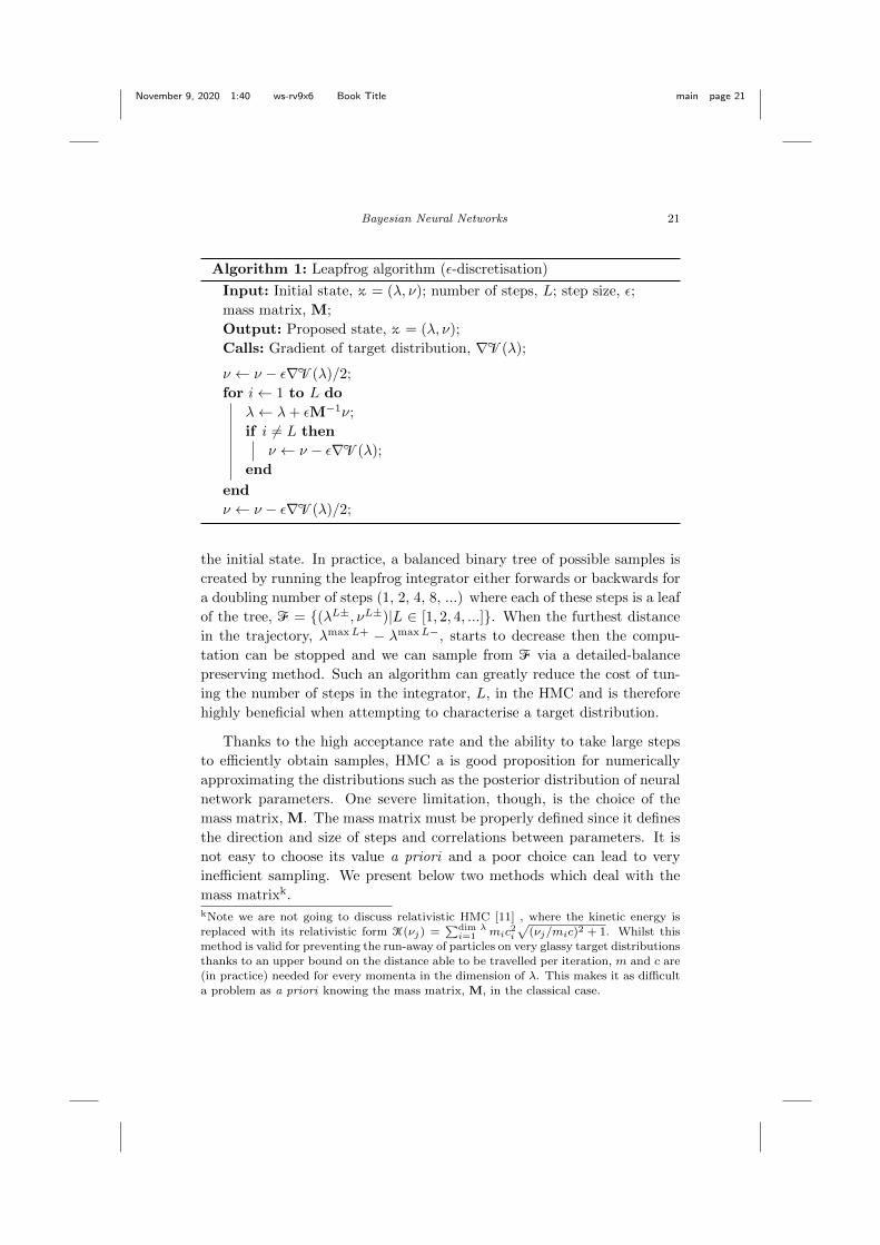
Algorithm 1: Leapfrog algorithm (ε-discretisation)
Input: Initial state, z = (λ, ν); number of steps, L; step size, ε;
mass matrix, M;
Output: Proposed state, z = (λ, ν);
Calls: Gradient of target distribution, ∇V(λ);
ν ← ν − ε∇V(λ)/2;
for i← 1 to L do
λ← λ+ εM−1ν;
if i 6= L then
ν ← ν − ε∇V(λ);
end
end
ν ← ν − ε∇V(λ)/2;
the initial state. In practice, a balanced binary tree of possible samples is
created by running the leapfrog integrator either forwards or backwards for
a doubling number of steps (1, 2, 4, 8, ...) where each of these steps is a leaf
of the tree, F= (λL±, νL±)|L ∈ [1, 2, 4, ...]. When the furthest distance
in the trajectory, λmaxL+ − λmaxL−, starts to decrease then the compu-
tation can be stopped and we can sample from F via a detailed-balance
preserving method. Such an algorithm can greatly reduce the cost of tun-
ing the number of steps in the integrator, L, in the HMC and is therefore
highly beneficial when attempting to characterise a target distribution.
Thanks to the high acceptance rate and the ability to take large steps
to efficiently obtain samples, HMC a is good proposition for numerically
approximating the distributions such as the posterior distribution of neural
network parameters. One severe limitation, though, is the choice of the
mass matrix, M. The mass matrix must be properly defined since it defines
the direction and size of steps and correlations between parameters. It is
not easy to choose its value a priori and a poor choice can lead to very
inefficient sampling. We present below two methods which deal with the
mass matrixk.kNote we are not going to discuss relativistic HMC [11] , where the kinetic energy is
replaced with its relativistic form K(νj) =∑dim λi=1 mic
2i
√(νj/mic)2 + 1. Whilst this
method is valid for preventing the run-away of particles on very glassy target distributionsthanks to an upper bound on the distance able to be travelled per iteration, m and c are
(in practice) needed for every momenta in the dimension of λ. This makes it as difficult
a problem as a priori knowing the mass matrix, M, in the classical case.
November 9, 2020 1:40 ws-rv9x6 Book Title main page 22
22 Charnock, Perreault-Levasseur, Lanusse
Quasi-Newtonian HMC [12] With quasi-Newtonian HMC (QNHMC)
we make use of the second order geometric information of the target distri-
bution as well as the gradient. The QNHMC modifies Hamilton’s equations
to
λ = BM−1ν (29)
ν = −B∇V(λ) (30)
where B is an approximation to the inverse Hessian derived using quasi-
Newton methods, for more details see [12]. Obtaining this approximation
of the Hessian is extremely efficient because all the necessary components
are calculated when solving Hamilton’s equations using leapfrog methods
as in algorithm 1. Note that the approximate inverse Hessian varies with
proposal, but is kept constant whilst solving Hamilton’s equations. The
inverse Hessian effectively rescales the momenta and parameters such that
each dimension has a similar scale and thus the movement around the target
distribution is more efficient with less correlated proposals. It is easiest to
begin with an initial inverse Hessian, B0 = I, and allow the adaptation of
the Hessian to the geometry of the space. Note that the mass matrix, M,
is still present to set the dynamical time-like scales of Hamilton’s equations
along each direction, but the rescaling of the momenta via B allows us to be
fairly ambiguous about its value. The optimal mass matrix for sampling is
equal to the covariance of the target distribution, but in practice, a diagonal
mass matrix with approximately correct variance values for the distribution
works well.
Example: Inference of the halo mass distribution function To
be able to extract cosmological information from the large scale structure
distribution of matter in the universe, such as the mass, location and clus-
tering of galaxies, obtained by galaxy surveys, we either have to summarise
the data into statistical quantities (such as the power spectrum, etc.) or
learn about the placement of all the objects in these surveys. Whilst the
first method is (potentially very) lossy, the complexity of the likelihood
describing the distribution of structures in the universe generally makes
the second technique intractable. With the goal of maximising the cosmo-
logical information extracted from galaxy surveys the Aquila consortium
has developed an algorithm for Bayesian origins reconstruction from galax-
ies (BORG) [13–15] which assumes a Bayesian hierarchical model to relate
Gaussian initial conditions of the early universe to the complex distribu-
tion of galaxies observed today. As part of this model, one needs to relate
November 9, 2020 1:40 ws-rv9x6 Book Title main page 23
Bayesian Neural Networks 23
P(δic|wcosmo)
δic
LPT(δic) p(wNPE)
wNPEδLPT
fwNPE,aNPE(δLPT)
ψ
p(wMDN)
wMDN
fwMDN,aMDN(ψ)
V(w, δic,wcosmo,Mobs)Mobs
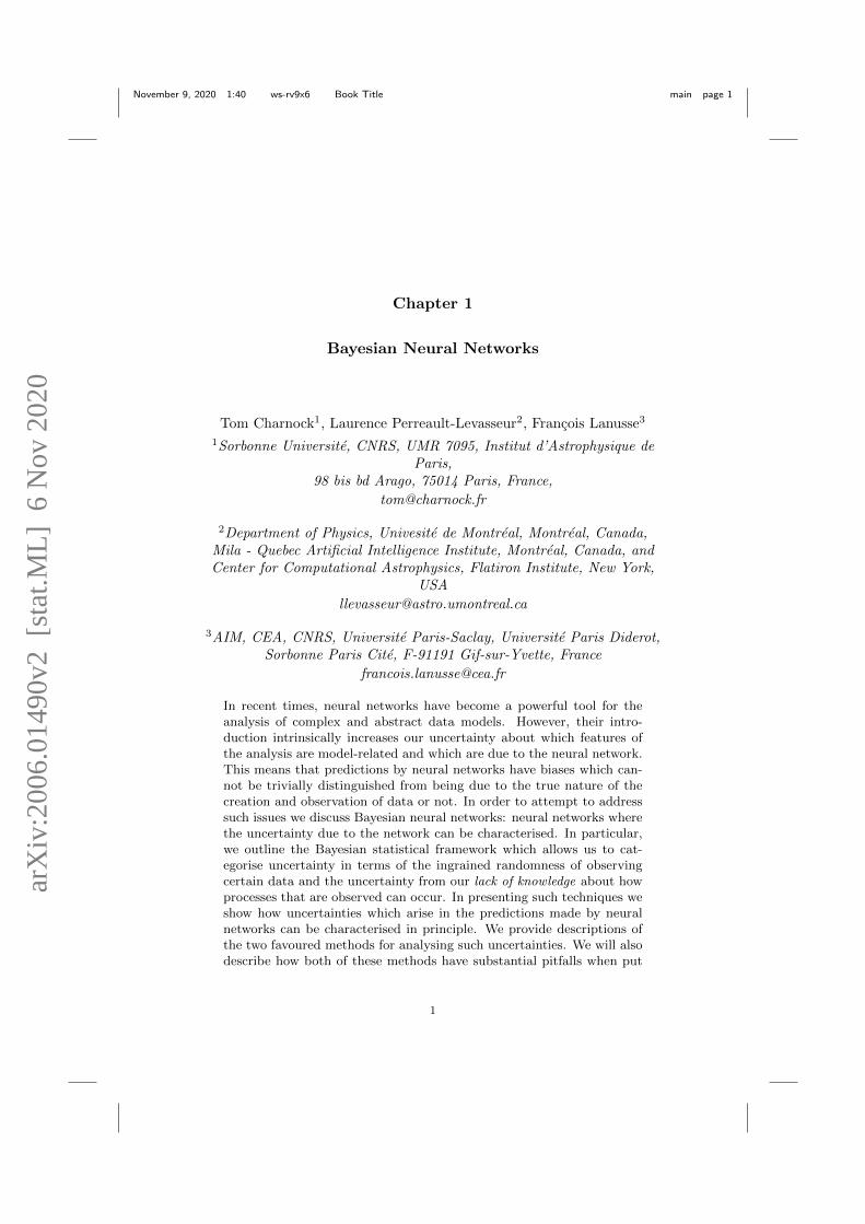
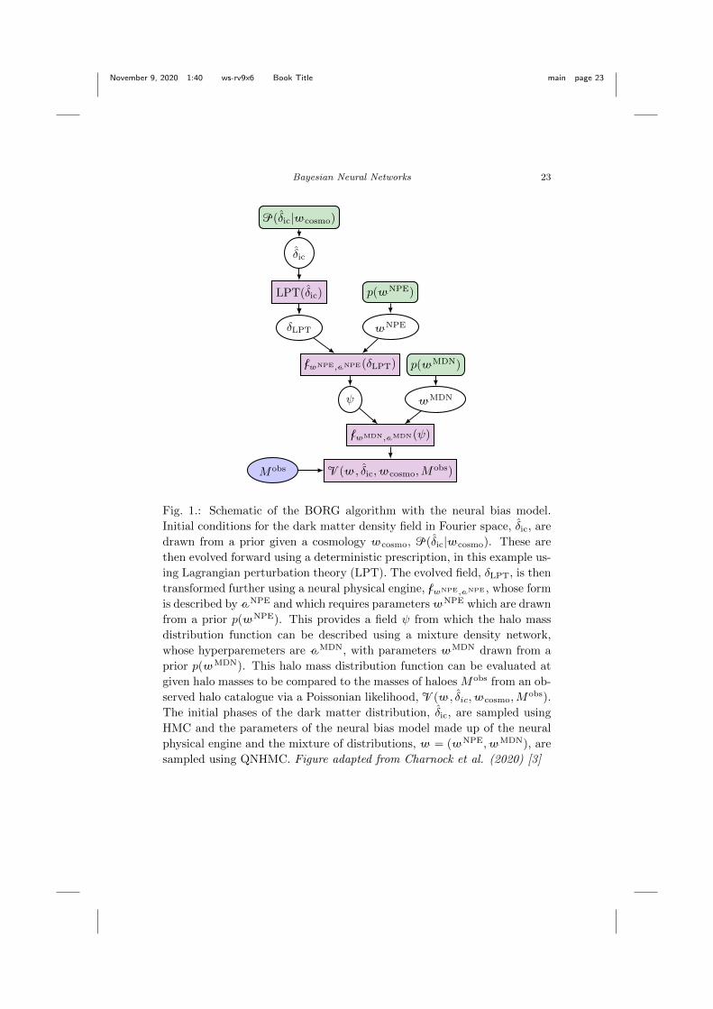
Fig. 1.: Schematic of the BORG algorithm with the neural bias model.
Initial conditions for the dark matter density field in Fourier space, δic, are
drawn from a prior given a cosmology wcosmo, P(δic|wcosmo). These are
then evolved forward using a deterministic prescription, in this example us-
ing Lagrangian perturbation theory (LPT). The evolved field, δLPT, is then
transformed further using a neural physical engine, fwNPE,aNPE , whose form
is described by aNPE and which requires parameters wNPE which are drawn
from a prior p(wNPE). This provides a field ψ from which the halo mass
distribution function can be described using a mixture density network,
whose hyperparemeters are aMDN, with parameters wMDN drawn from a
prior p(wMDN). This halo mass distribution function can be evaluated at
given halo masses to be compared to the masses of haloes Mobs from an ob-
served halo catalogue via a Poissonian likelihood, V(w, δic,wcosmo,Mobs).
The initial phases of the dark matter distribution, δic, are sampled using
HMC and the parameters of the neural bias model made up of the neural
physical engine and the mixture of distributions, w = (wNPE,wMDN), are
sampled using QNHMC. Figure adapted from Charnock et al. (2020) [3]
November 9, 2020 1:40 ws-rv9x6 Book Title main page 24
24 Charnock, Perreault-Levasseur, Lanusse
observed galaxies to the underlying, and otherwise invisible, dark matter
field through a so-called bias model, which is an effective description for
extremely complex astrophysical effects. Finding a flexible enough and yet
tractable parameterisation for this model a priori is a difficult task.
Using physical considerations, such as locality and radial symmetry, to
reduce the numbers of degrees of freedom, a very simple mixture density
network with 17 parameters was proposed to model this bias [3]. This net-
work, dubbed a neural physical engine due to its physical inductive biases,
is small enough that each parameter is exactly identifiable, so that sensible
priors could be defined for those parameters. The ability to place these
meaningful priors on network parameters is well motivated for this physi-
cally motivated problem, but may be more difficult to design for problems
without physical intuition.
10131012 1014 1015
Mass [Mʘ]
n(M|δ
)
10−20
10−19
10−18
10−17
10−16
10−15
10−14
10−13
δ=−0.69δ=−0.58δ=−0.43δ=−0.22δ=0.06δ=0.45
δ=0.98δ=1.71δ=2.71δ=4.08δ=5.95δ=8.52
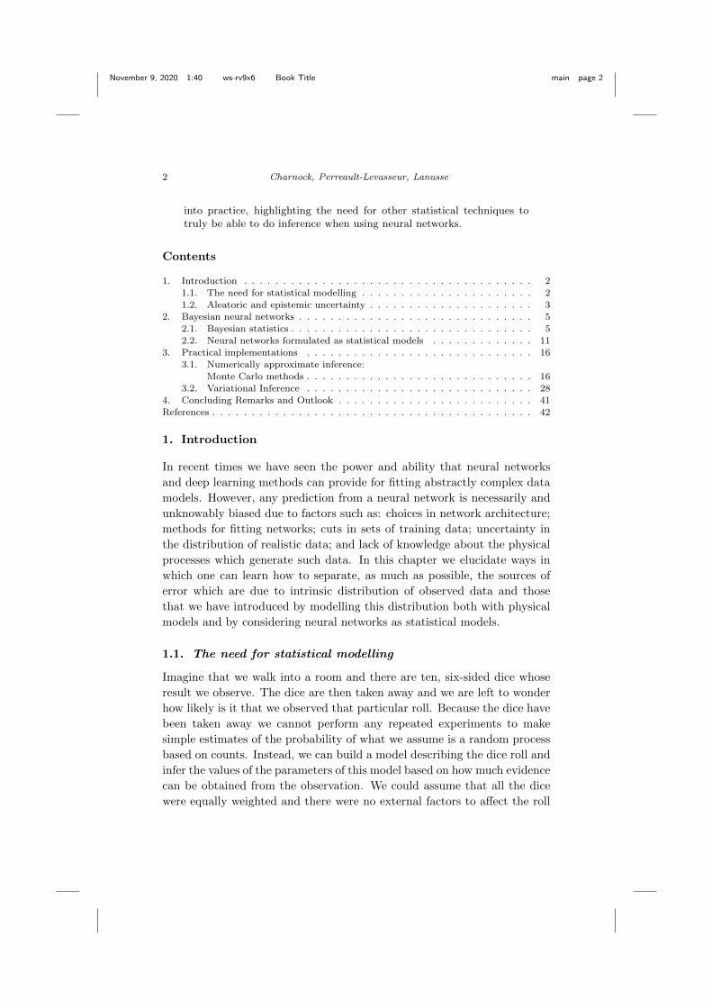
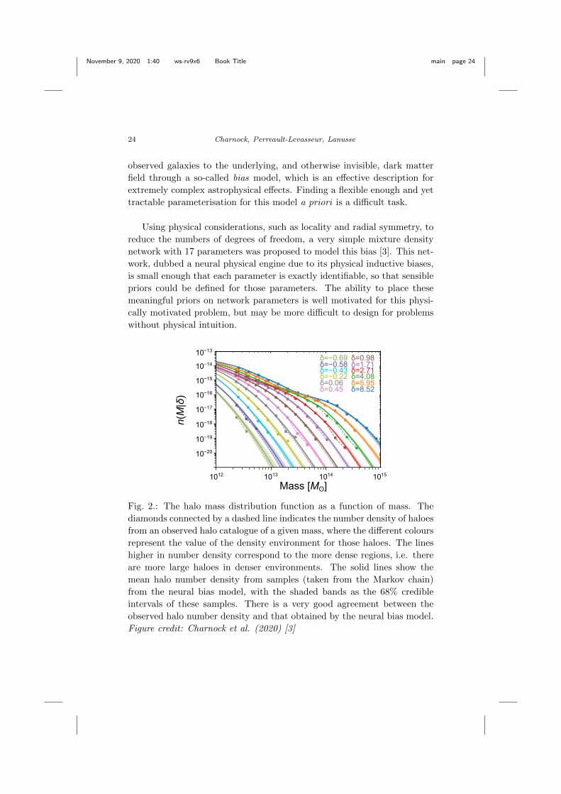
Fig. 2.: The halo mass distribution function as a function of mass. The
diamonds connected by a dashed line indicates the number density of haloes
from an observed halo catalogue of a given mass, where the different colours
represent the value of the density environment for those haloes. The lines
higher in number density correspond to the more dense regions, i.e. there
are more large haloes in denser environments. The solid lines show the
mean halo number density from samples (taken from the Markov chain)
from the neural bias model, with the shaded bands as the 68% credible
intervals of these samples. There is a very good agreement between the
observed halo number density and that obtained by the neural bias model.
Figure credit: Charnock et al. (2020) [3]
November 9, 2020 1:40 ws-rv9x6 Book Title main page 25
Bayesian Neural Networks 25
Sampling from this model could also be integrated within the larger
hierarchical model of the BORG framework using QNHMC (see figure 1
for a description of the BORG+neural bias model algorithm). Concretely,
BORG was run in two blocks, first using HMC to propose samples of the
dark matter density field and then using QNHMC to propose possible neu-
ral bias models. The target distribution was assumed to be a Poissionian
sampling of the number density of haloes in any particular environment
as described by a mixture density network, fwMDN,aMDN(ψ), evaluated at
possible halo masses, m, and the summarised environmental properties,
ψ = fwNPE,aNPE(δLPT), given by the neural physical engine. The parame-
ters in the target likelihood for the masses of haloes in a halo catalogue can
be explicitly written in terms of the output of the mixture density network,
i.e. αι,ih(ψ(δLPT,ih ,w
NPE),wMDN), µι,ih
(psi(δLPT,ih ,w
NPE),wMDN)
and σι,ih(ψ(δLPT,ih ,w
NPE),wMDN)
where i labels the number of voxels
in the simulator, h labels the number of halos in the catalogue and ι labels
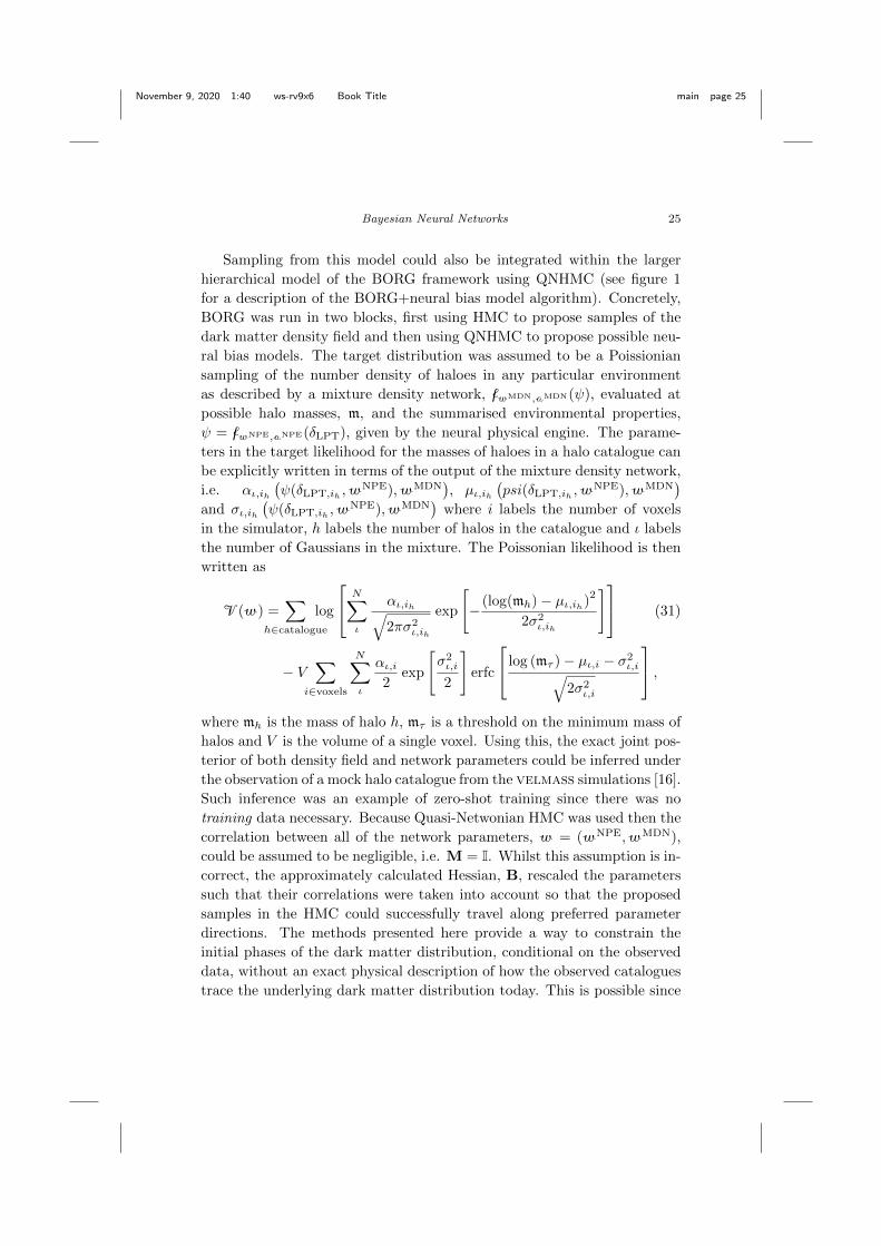
the number of Gaussians in the mixture. The Poissonian likelihood is then
written as
V(w) =∑
h∈catalogue
log
N∑ι
αι,ih√2πσ2
ι,ih
exp
[− (log(mh)− µι,ih)
2
2σ2ι,ih
] (31)
− V∑
i∈voxels
N∑ι
αι,i2
exp
[σ2ι,i
2
]erfc
log (mτ )− µι,i − σ2ι,i√
2σ2ι,i
,where mh is the mass of halo h, mτ is a threshold on the minimum mass of
halos and V is the volume of a single voxel. Using this, the exact joint pos-
terior of both density field and network parameters could be inferred under
the observation of a mock halo catalogue from the velmass simulations [16].
Such inference was an example of zero-shot training since there was no
training data necessary. Because Quasi-Netwonian HMC was used then the
correlation between all of the network parameters, w = (wNPE,wMDN),
could be assumed to be negligible, i.e. M = I. Whilst this assumption is in-
correct, the approximately calculated Hessian, B, rescaled the parameters
such that their correlations were taken into account so that the proposed
samples in the HMC could successfully travel along preferred parameter
directions. The methods presented here provide a way to constrain the
initial phases of the dark matter distribution, conditional on the observed
data, without an exact physical description of how the observed catalogues
trace the underlying dark matter distribution today. This is possible since
November 9, 2020 1:40 ws-rv9x6 Book Title main page 26
26 Charnock, Perreault-Levasseur, Lanusse
we can use the neural bias model to map from the dark matter distribu-
tion to some unknown function that describes how a catalogue of observed
halos traces the underlying dark matter based on some physical principles.
These physical principles are built directly into the neural physical engine.
Any uncertainty in the form of this description can then be marginalised
out since the distribution of the parameters in the neural bias model is
available via the samples obtained in the QNHMC.
Riemannian Manifold HMC [17] Whilst we have so far depended on
a choice of mass matrix to set the time-like steps in the integrator, it is
possible to exploit the geometry of the Hamiltonian to adaptively avoid
having to choose. Samples from the Hamiltonian are effectively points in
a Riemannian surface with a metric defined by the Fisher information of
the target distribution, I(λ) = 〈∇%(λ′|χ)(∇%(λ′|χ))T 〉λ. Since the Fisher
information describes the amount of information a random observable, χ,
contains about any model parameters λ, then the parameter space has
larger curvature wherever there is a lot of support from the data. In essence,
this metric is a position-dependent equivalent to the mass matrix which
we have so far considered, but since we have to calculate ∇%(λ|χ) in the
integrator anyway, we can actually approximate the Fisher information
cheaply. However, to ensure that the Hamiltonian is still the logarithm of
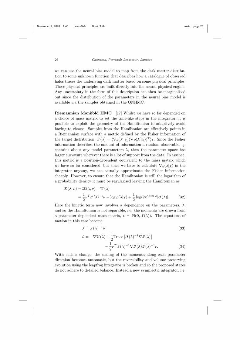
a probability density it must be regularised leaving the Hamiltonian as
H(λ, ν) = K(λ, ν) + V(λ)
=1
2νTI(λ)−1ν − log %(λ|χ) +
1
2log(2π)dim λ|I(λ)|. (32)
Here the kinetic term now involves a dependence on the parameters, λ,
and so the Hamiltonian is not separable, i.e. the momenta are drawn from
a parameter dependent mass matrix, ν ∼ N(0,I(λ)). The equations of
motion in this case become
λ = I(λ)−1ν (33)
ν = −∇V(λ) +1
2Trace
[I(λ)−1∇I(λ)
]− 1
2νTI(λ)−1∇I(λ)I(λ)−1ν. (34)
With such a change, the scaling of the momenta along each parameter
direction becomes automatic, but the reversibility and volume preserving
evolution using the leapfrog integrator is broken and so the proposed states
do not adhere to detailed balance. Instead a new symplectic integrator, i.e.
November 9, 2020 1:40 ws-rv9x6 Book Title main page 27
Bayesian Neural Networks 27
an integrator for Hamiltonian systems, is required to make the volume pre-
serving transformation of the momenta (by calculating the Jacobian of the
inverse Fisher matrix) such that Hamilton’s equations can be solved. Whilst
this adds extra complexity to the equations of motion, it is equivalent to
only two additional steps in the integrator since the Fisher information can
be approximated cheaply from the calculation of the gradient of the poten-
tial energy. By using the RMHMC, we avoid the need to choose a mass
matrix (or approximate the Hessian). ε can be fixed to some value as the
adaptive matrix is able to overcome the step size, and L, i.e. the number
of steps in the integrator, can be chosen to tune the acceptance rate.
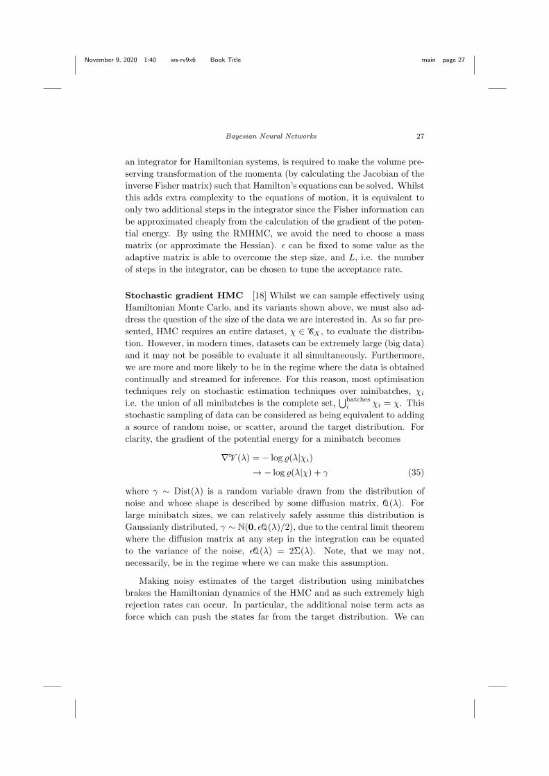
Stochastic gradient HMC [18] Whilst we can sample effectively using
Hamiltonian Monte Carlo, and its variants shown above, we must also ad-
dress the question of the size of the data we are interested in. As so far pre-
sented, HMC requires an entire dataset, χ ∈ EX , to evaluate the distribu-
tion. However, in modern times, datasets can be extremely large (big data)
and it may not be possible to evaluate it all simultaneously. Furthermore,
we are more and more likely to be in the regime where the data is obtained
continually and streamed for inference. For this reason, most optimisation
techniques rely on stochastic estimation techniques over minibatches, χii.e. the union of all minibatches is the complete set,
⋃batchesi χi = χ. This
stochastic sampling of data can be considered as being equivalent to adding
a source of random noise, or scatter, around the target distribution. For
clarity, the gradient of the potential energy for a minibatch becomes
∇V(λ) = − log %(λ|χi)→ − log %(λ|χ) + γ (35)
where γ ∼ Dist(λ) is a random variable drawn from the distribution of
noise and whose shape is described by some diffusion matrix, Q(λ). For
large minibatch sizes, we can relatively safely assume this distribution is
Gaussianly distributed, γ ∼ N(0, εQ(λ)/2), due to the central limit theorem
where the diffusion matrix at any step in the integration can be equated
to the variance of the noise, εQ(λ) = 2Σ(λ). Note, that we may not,
necessarily, be in the regime where we can make this assumption.
Making noisy estimates of the target distribution using minibatches
brakes the Hamiltonian dynamics of the HMC and as such extremely high
rejection rates can occur. In particular, the additional noise term acts as
force which can push the states far from the target distribution. We can
November 9, 2020 1:40 ws-rv9x6 Book Title main page 28
28 Charnock, Perreault-Levasseur, Lanusse
reduce this effect by taking further inspiration from mechanical systems
- we can use Langevin dynamics to describe the macroscopic states of a
statistical mechanical system with a stochastic noise term describing the
expected effect of some ensemble of microscopic states. In particular, us-
ing second-order Langevin equations is equivalent to including a friction
term which decreases the energy and, thus, counterbalances the effect of
the noise. Equations 25 and 26 therefore get promoted to
λ = M−1ν (36)
ν = −∇V(λ)− Q(λ)M−1ν + γ (37)
Solving these equations provides a stationary distribution, π(λ, ν) ≈H(λ, ν), with the distribution of samples, λ ∼ ρχ, i.e. λ is drawn with
probability ρ(λ|χ). Of course, this method depends on knowing the dis-
tribution of the noise well, but for large minibatch sizes, this approaches
Gaussian. The stochastic gradient HMC, in this case, provides a way to
obtain samples from the target distribution even when not using the entire
dataset and therefore vastly reducing computational expense and allowing
for active collection and inference of data.
3.2. Variational Inference
Whilst a target probability distribution can be approximately characterised
by obtaining exact samples from the distribution via Monte Carlo methods,
it is often a very costly process. Instead we can use variational inference,
where a variational distribution, say qm(λ|χ), is chosen to represent a
very close approximation to the target distribution, ρ(λ|χ). In general,
qm(λ|χ) is a tractable distribution, parameterised by some m, and via the
optimisation of these parameters qm(λ|χ) can hopefully be made close to
the target distribution, ρ(λ|χ). Note, again, that if the target distribution
is the posterior predictive distribution of some model, p(y|x), then fitting
a variational distribution to this is not a Bayesian procedure in the same
way that maximum likelihood estimation is not Bayesian.
To describe what is meant by close in the context of distributions we
often consider the Kullback-Leibler (KL) divergence (or relative entropy).
In a statistical setting, the KL-divergence is a measure of information lost
when approximating a distribution ρ(λ|χ) with some other qm(λ|χ),
KL(ρ||qm) =
∫EΛ
dλ ρ(λ|χ) logρ(λ|χ)
qm(λ|χ). (38)
November 9, 2020 1:40 ws-rv9x6 Book Title main page 29
Bayesian Neural Networks 29
When KL(ρ||qm) = 0, there is no information loss and so ρ(λ|χ) and
qm(λ|χ) are equivalent. Values KL(ρ||qm) > 0 indicate the degree of
information lost. Note that the KL-divergence is not symmetric and as
such is not a real distance metric.
The form of (38) assumes the integral of ρ(λ|χ) to be tractable. In
fact, in the case that the expectation can be approximated well, we can use
the KL-divergence to perform expectation propagation. However, if we are
considering the approximation of the posterior distribution of network pa-
rameters, as stated in section 2, we can expect the integral of pa(w|x, y) to
be intractable meaning that calculating KL(pa||qm) would be necessarily
hard. Instead we can consider the reverse KL-divergence
KL(qm||ρ) =
∫EΛ
dλqm(λ|χ) logqm(λ|χ)
ρ(λ|χ). (39)
The choice of qm(λ|χ) is specified so that expectations are tractable. How-
ever, evaluating ρ(λ|χ) would require calculating the evidence, e(χ), which,
although constant for different λ, remains intractable. For convenience we
can consider the unnormalised distribution (as we did for detailed balance
in section 3.1.1)
%(λ|χ) = L(χ|λ)p(λ)
= ρ(λ|χ)e(χ)
= p(χ, λ), (40)
and calculate a new measure
ELBO(qm) = −∫EΛ
dλqm(λ|χ) logqm(λ|χ)
%(λ|χ). (41)
Note that this has the form of minus the reverse KL-divergence, but is not
equivalent since %(λ|χ) is not normalised. By substitution we can see that
ELBO(qm) = −∫EΛ
dλqm(λ|χ) logqm(λ|χ)
ρ(λ|χ)e(χ)
= −∫EΛ
dλqm(λ|χ) logqm(λ|χ)
ρ(λ|χ)+ log e(χ)
= −KL(qm||ρ) + log e(χ). (42)
Since log e(χ) is constant with respect to the parameters, λ, maximising
ELBO(qm) will force qm(λ|χ) close to the target distribution ρ(λ|χ). The
term ELBO comes from the fact that the KL-divergence is non-negative
and so ELBO(qm) defines a lower bound to the evidence, e(χ).
November 9, 2020 1:40 ws-rv9x6 Book Title main page 30
30 Charnock, Perreault-Levasseur, Lanusse
3.2.1. Mean-field variation
One efficient way of parameterising a distribution for approximating a tar-
get, ρ(λ|χ), is to make it factorise along each dimension of the parameters,
i.e.
qm(λ|χ) =
dimλ∏i=1
qmi (λi|χ). (43)
In doing such, the ELBO for any individual qmj is
ELBO(qmj ) =
∫· · ·∫
EΛ,j
dλj∏i
qmi (λi|χ)×
[log %(λ|χ)−
∑k
log qmk (λk|χ)
]
=
∫EΛ,j
dλj qmj (λj |χ)
∫· · ·∫
EΛ,i 6=j
dλi∏i6=j
qmi (λi|χ)
×
[log %(λ|χ)−
∑k
log qmk (λk|χ)
]
=
∫EΛ,j
dλj qmj (λj |χ)×
[Ei 6=j
[log %(λj |χ)]− log qmj (λj |χ)
]+ const (44)
where the constant is the expectation value of the factorised distributions,
qmi (λi|χ), in the dimensions where i 6= j and is unimportant for the op-
timisation of the distribution for the jth dimension since it is independent
of λj . Ei 6=j [log %(λj |χ)] is the expectation value of the logarithm of the
target distribution for every qmi (λi|χ) where i 6= j, and remains due to its
dependence on λj . The optimal jth distribution is the one that maximises
the ELBO which is equivalent to optimising each of the factorised distri-
butions, qmj (λj |χ), in turn to obtain qm
j (λj |χ) = exp [Ei6=j [log %(λj |χ)]].
This provides a mean-field approximation of the target distribution.
3.2.2. Bayes by Backprop
Bayes by Backprop [19, 20] (a form of stochastic gradient variational Bayes)
provides a method for approximating a target distribution, ρ(λ|χ), using
differentiable functions such as neural networks. The basic premise of Bayes
by Backprop relies on a technique known as the reparameterisation trick [21,
22] . The reparametrisation trick provides a method of drawing random
samples, w, from a Gaussian distribution, whilst allowing the samples to be
November 9, 2020 1:40 ws-rv9x6 Book Title main page 31
Bayesian Neural Networks 31
differentiable with respect to the parameters of the Gaussian distribution
(mean and standard deviation, m = (µ, σ)). This can be achieved by
reparameterising N(µi, σi) in terms of an independent normally distributed
auxiliary variable, ε ∼N(0, 1), i.e.
w(mi) ∼ N(µi, σi)
= µi + σiεi. (45)
Here, we can view w(mi) as the ith random variable parameter of a neural
network with a total of nw network parameters where w(m) = w(mi)| i ∈[1, nw]. Any evaluation of the neural network is a sample λ ∼ qm
χ,w,
i.e. λ is drawn with probability qm(λ|χ,w). Maximising the ELBO (42),
between qm(λ|χ,w) and an unnormalised target distribution, %(λ|χ), can
now be done via backpropagation since we can calculate
∂mELBO(qm) =
(∂w(m)ELBO(qm) + ∂µELBO(qm)
(ε/σ)∂w(m)ELBO(qm) + ∂σELBO(qm)
)(46)
and update the parameters using
m← m− η∂mELBO(qm) (47)
where η is a learning rate. Note that the ∂w(m)ELBO(qm) terms in (47) are
exactly the same as the gradients normally associated with backpropagation
in neural networks.
As originally presented, Bayes by Backprop was an attempt to make
Bayesian posterior predictions of targets, y, from inputs, x, as in (12),
where ρ(w|xtrain, ytrain) ≡∏nw
i=1 N(µi, σi). Here, the values of all µi and
σi are fit using maximum likelihood estimation (or maximum a posterior
estimation) given data xtrain and ytrain. As explained in section 2.2, the
distribution of weights, pa(w), is likely to be extremely non-trivial, since
most network parameters are non-identifiable and highly degenerate with
other parameters. Therefore, modelling this distribution as a Gaussian is
unlikely to be very accurate. This can, therefore, incorrectly conflate the
epistemic uncertainty for y from a particular network, a, with parame-
ters, w, and input, x, with the posterior prediction. In essence, Bayes by
Backprop provides a way of sampling from a single choice of an (arbitrarily
complex) approximation of a target distribution much more efficiently than
using numerical schemes such as Markov methods, but there is little knowl-
edge in how close this approximation is to the desired target. By fitting
the parameters, m, of the neural distribution rather than characterising
their distribution, p(m), the characterisation of the epistemic uncertainty
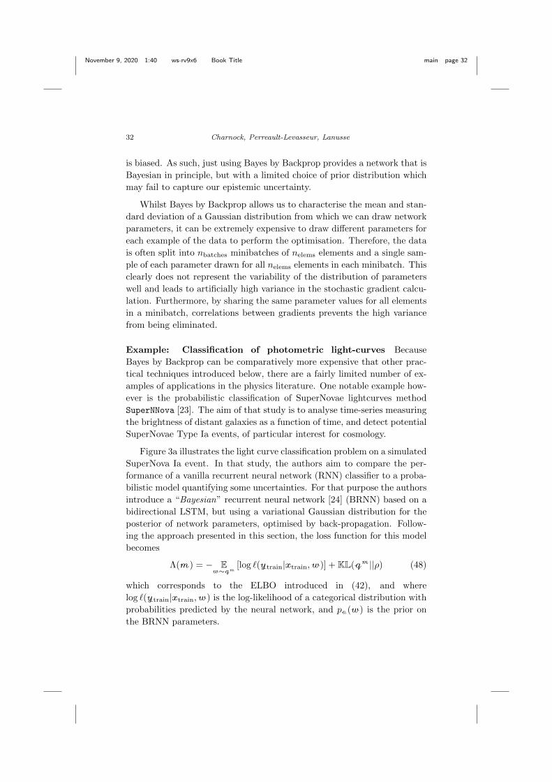
November 9, 2020 1:40 ws-rv9x6 Book Title main page 32
32 Charnock, Perreault-Levasseur, Lanusse
is biased. As such, just using Bayes by Backprop provides a network that is
Bayesian in principle, but with a limited choice of prior distribution which
may fail to capture our epistemic uncertainty.
Whilst Bayes by Backprop allows us to characterise the mean and stan-
dard deviation of a Gaussian distribution from which we can draw network
parameters, it can be extremely expensive to draw different parameters for
each example of the data to perform the optimisation. Therefore, the data
is often split into nbatches minibatches of nelems elements and a single sam-
ple of each parameter drawn for all nelems elements in each minibatch. This
clearly does not represent the variability of the distribution of parameters
well and leads to artificially high variance in the stochastic gradient calcu-
lation. Furthermore, by sharing the same parameter values for all elements
in a minibatch, correlations between gradients prevents the high variance
from being eliminated.
Example: Classification of photometric light-curves Because
Bayes by Backprop can be comparatively more expensive that other prac-
tical techniques introduced below, there are a fairly limited number of ex-
amples of applications in the physics literature. One notable example how-
ever is the probabilistic classification of SuperNovae lightcurves method
SuperNNova [23]. The aim of that study is to analyse time-series measuring
the brightness of distant galaxies as a function of time, and detect potential
SuperNovae Type Ia events, of particular interest for cosmology.
Figure 3a illustrates the light curve classification problem on a simulated
SuperNova Ia event. In that study, the authors aim to compare the per-
formance of a vanilla recurrent neural network (RNN) classifier to a proba-
bilistic model quantifying some uncertainties. For that purpose the authors
introduce a “Bayesian” recurrent neural network [24] (BRNN) based on a
bidirectional LSTM, but using a variational Gaussian distribution for the
posterior of network parameters, optimised by back-propagation. Follow-
ing the approach presented in this section, the loss function for this model
becomes
Λ(m) = − Ew∼qm
[log `(ytrain|xtrain,w)] + KL(qm||ρ) (48)
which corresponds to the ELBO introduced in (42), and where
log `(ytrain|xtrain,w) is the log-likelihood of a categorical distribution with
probabilities predicted by the neural network, and pa(w) is the prior on
the BRNN parameters.
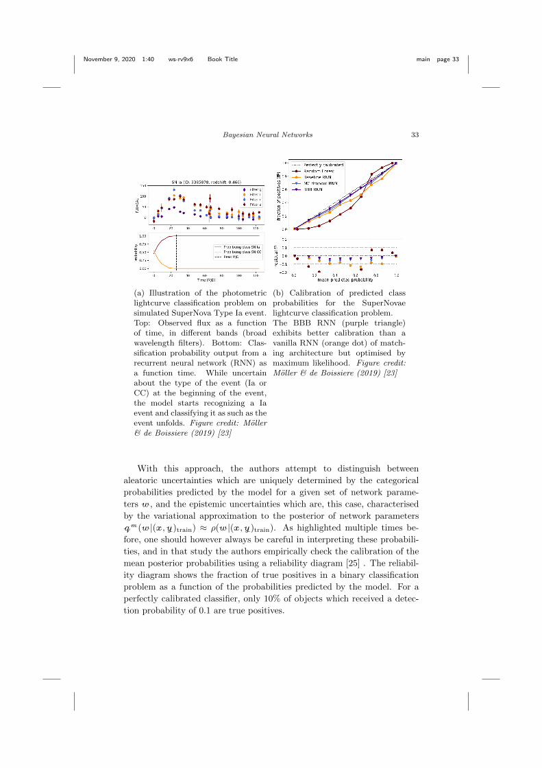
November 9, 2020 1:40 ws-rv9x6 Book Title main page 33
Bayesian Neural Networks 33
(a) Illustration of the photometriclightcurve classification problem onsimulated SuperNova Type Ia event.Top: Observed flux as a functionof time, in different bands (broadwavelength filters). Bottom: Clas-sification probability output from arecurrent neural network (RNN) asa function time. While uncertainabout the type of the event (Ia orCC) at the beginning of the event,the model starts recognizing a Iaevent and classifying it as such as theevent unfolds. Figure credit: Moller& de Boissiere (2019) [23]
(b) Calibration of predicted classprobabilities for the SuperNovaelightcurve classification problem.The BBB RNN (purple triangle)exhibits better calibration than avanilla RNN (orange dot) of match-ing architecture but optimised bymaximum likelihood. Figure credit:Moller & de Boissiere (2019) [23]
With this approach, the authors attempt to distinguish between
aleatoric uncertainties which are uniquely determined by the categorical
probabilities predicted by the model for a given set of network parame-
ters w, and the epistemic uncertainties which are, this case, characterised
by the variational approximation to the posterior of network parameters
qm(w|(x, y)train) ≈ ρ(w|(x, y)train). As highlighted multiple times be-
fore, one should however always be careful in interpreting these probabili-
ties, and in that study the authors empirically check the calibration of the
mean posterior probabilities using a reliability diagram [25] . The reliabil-
ity diagram shows the fraction of true positives in a binary classification
problem as a function of the probabilities predicted by the model. For a
perfectly calibrated classifier, only 10% of objects which received a detec-
tion probability of 0.1 are true positives.
November 9, 2020 1:40 ws-rv9x6 Book Title main page 34
34 Charnock, Perreault-Levasseur, Lanusse
Figure 3b shows this calibration diagram for different classifiers, but of
particular interest are the curves for the baseline RNN and BBB RNN,
in both cases the actual neural network architecture is identical, but the
former is optimised to find the maximum likelihood estimates of the network
parameters, while the later is trained by Bayes by Backprop. The BBB
RNN predicted probabilities are closer to the diagonal representing a more
correct calibration than the baseline RNN. In this example including a
model for the epistemic uncertainties improves the model calibration.
3.2.3. Local reparameterisation trick
Although for large numbers of network parameters, nw, characterising the
global uncertainty of the parameters using the reparameterisation trick be-
comes computationally unfeasible for each element of data and for each
parameter in the network, a local noise approximation [26] can be made to
transform the perturbation of parameters to a perturbation of activation
values
oljn ∼ N
(dim l−1∑i=1
µljial−1in ,
dim l−1∑i=1
(σlji)2 (
al−1in
)2), (49)
where aljn = f(oljn) is the activated output (with possibly non-linear acti-
vation function f) of the jth unit of the lth layer of a neural network with
nl layers, according to the nth element of the input minibatch. As with the
reparameterisation trick, the sampling of the activation value of any layer
can be written as
oljn =
dim l−1∑i=1
µljial−1in + εljn
√(σlji)2 (
al−1in
)2(50)
where εljn ∼ N(0, 1). Whilst the parameters mlji = (µlji, σ
lji) of the Gaus-
sian distribution describe the probabilistic model for a network parameter,
w(mlji), from unit i of layer l − 1 to unit j of layer l, this model is never
sampled, and only the activation values are sampled. The dimensional-
ity of the probabilistic interpretation of layer outputs, i.e. the number of
ε = εlin| i ∈ [1,dim l], l ∈ [1, nl], n ∈ [1, nelems] needed to be stored for
computation of the gradient is much lower than when considering the num-
ber of random draws needed for every single network parameter and every
element of data in the minibatch. Furthermore, the variance of the gradi-
ent is much less when using the local reparameterisation trick than when
assuming a single random draw for each parameter being the same for all
of the elements of data in a minibatch.
November 9, 2020 1:40 ws-rv9x6 Book Title main page 35
Bayesian Neural Networks 35
3.2.4. Variational dropout
One limitation of the local reparameterisation trick is that it only applies
to networks with no weight sharing, i.e. fully-connected neural networks.
However, inspired by the local reparameterisation trick, a general method
for approximating distributions using multiplicative noise can be imple-
mented. Variational dropout [27, 28] is another way of approximating a
target distribution, ρ(λ|χ) with qm(λ|χ,w). In this case, the distribution
is defined by the application of random variables to the outputs of hidden
layers in a neural network. Much like the local reparameterisation trick,
the outputs of the nl layers of a neural network are draws from some mul-
tiplicative noise model, alin = εlinf(olin), where olin are the non-activated
outputs of the lth layer of a neural network at element n in the minibatch.
Note that olin can be obtained using any function, i.e. fully connected,
convolutional, etc. f is some (possibly non-linear) activation function and
εlin ∼ Dist(mlin) is a random variable drawn from some distribution pa-
rameterised by some m = mlin| i ∈ [1,dim l], l ∈ [1, nl], n ∈ [1, nelems].
Selecting some form for the distribution and values for its parameters, m,
provides a way of obtaining samples from the neural network by running the
network forward with many draws of ε. This makes the network a model
of a Bayesian neural network rather than a Bayesian neural network itself
- there is no sampling of the parameters of the network, and no attempt
to characterise their uncertainty. Furthermore, the value of m cannot be
fit using Bayes by Backprop and it is an a priori choice for the sampling
distributionl.
Bernoulli dropout One method of performing variational dropout is by
using ε ∼ Bernoulli(m), which amounts to feeding forward an input to a
network with dropout [29] with a keep rate m for each of the outputs of
each layer of the neural network multiple times. The outputted samples
can then be interpreted as the distribution of possible targets which can be
obtained using that network (and the choice of the Bernoulli distribution
with parameters m). It is very common to set all values of mlin ∈ m to the
same value, although it can be optimised via expectation maximisation.
The ease with which this method can be implemented has made it very
popular, and in the limit of large number of samples, the activated outputs
approach a Gaussian distribution thanks to the central limit theorem. Note
lIt should be noted that the parameters, m, of any variational dropout distribution canbe optimised via expectation maximisation.
November 9, 2020 1:40 ws-rv9x6 Book Title main page 36
36 Charnock, Perreault-Levasseur, Lanusse
that the choice of a Bernoulli distribution changes the expected output of
any activation layer as 〈alin〉 = mlin(1−ml
in)alin, therefore there is a scaling
which needs to be taken into account.
Gaussian dropout A second option is to draw the random variable from
a unit-mean Gaussian [26, 30], ε ∼ N(I,diag(m)), so that the expectation
value of the multiplication of the output of a unit of a layer by the random
variable remains, 〈alin〉 = alin the same since 〈ε〉 = 1. Furthermore, by
calculating the variational objective the value of m in the multiplicative
noise distribution can be fit using expectation maximisation.
For both the Bernoulli, Gaussian or any other multiplicative dropout
distribution, by maximising the ELBO(qm), we can get qm(λ|χ,w) close
to ρ(λ|χ) allowing us to make estimates of this distribution. Again it should
be stated that this is not Bayesian in the sense that if the variational dis-
tribution provided by variational dropout is approximating the posterior
predictive distribution, p(y|x), there is no sense of certainty in how good
that approximation is. There is no attempt to characterise our lack of
knowledge of the parameters of the network or the parameters of the dis-
tributions, mm.
3.2.5. Monte Carlo Dropout
Very closely related to Bernoulli variational dropout, is the MC Dropout
model [27]. Completely similar to the previous section, MC Dropout pro-
vides a Bayesian framework to interpret the effect of traditional dropout [29]
on neural networks. A variational distribution qm(w|χ, λ) assumed for the
network parameter posterior can be parameterised as w = M ·diag([zj ]Jj=1)
with zj ∼ Bernoulli(m), M being a K × J weight matrix, and m being
the dropout rate. Given this formulation for the variational distribution it
can be shown that a KL divergence with respect to an implicit prior can
be approximated as a simple `2 regularisation term [27]. Training a neural
network under dropout and with `2 weight regularization therefore max-
imising the ELBO(qm) and is performing proper variational inference at
no extra cost.
Example: Probabilistic classification of galaxy morphologies and
active learning MC Dropout is the most frequent solution adopted formOf course, if considering a MAP estimate, then some characterisation of our lack ofknowledge is taken into account, but the distribution is still neglected.
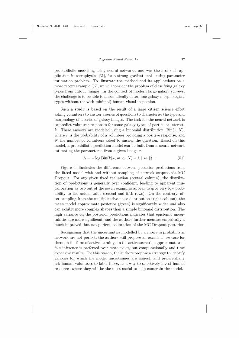
November 9, 2020 1:40 ws-rv9x6 Book Title main page 37
Bayesian Neural Networks 37
probabilistic modelling using neural networks, and was the first such ap-
plication in astrophysics [31], for a strong gravitational lensing parameter
estimation problem. To illustrate the method and its applications on a
more recent example [32], we will consider the problem of classifying galaxy
types from cutout images. In the context of modern large galaxy surveys,
the challenge is to be able to automatically determine galaxy morphological
types without (or with minimal) human visual inspection.
Such a study is based on the result of a large citizen science effort
asking volunteers to answer a series of questions to characterise the type and
morphology of a series of galaxy images. The task for the neural network is
to predict volunteer responses for some galaxy types of particular interest,
k. These answers are modeled using a binomial distribution, Bin(r, N),
where r is the probability of a volunteer providing a positive response, and
N the number of volunteers asked to answer the question. Based on this
model, a probabilistic prediction model can be built from a neural network
estimating the parameter r from a given image x:
Λ = − log Bin(k|x,w,a, N) + λ ‖ w ‖22 . (51)
Figure 4 illustrates the difference between posterior predictions from
the fitted model with and without sampling of network outputs via MC
Dropout. For any given fixed realisation (central column), the distribu-
tion of predictions is generally over confident, leading to apparent mis-
calibration as two out of the seven examples appear to give very low prob-
ability to the actual value (second and fifth rows). On the contrary, af-
ter sampling from the multiplicative noise distribution (right column), the
mean model approximate posterior (green) is significantly wider and also
can exhibit more complex shapes than a simple binomial distribution. The
high variance on the posterior predictions indicates that epistemic uncer-
tainties are more significant, and the authors further measure empirically a
much improved, but not perfect, calibration of the MC Dropout posterior.
Recognising that the uncertainties modelled by a choice in probabilistic
network are not perfect, the authors still propose an excellent use case for
them, in the form of active learning. In the active scenario, approximate and
fast inference is preferred over more exact, but computationally and time
expensive results. For this reason, the authors propose a strategy to identify
galaxies for which the model uncertainies are largest, and preferentially
ask human volunteers to label those, as a way to selectively invest human
resources where they will be the most useful to help constrain the model.
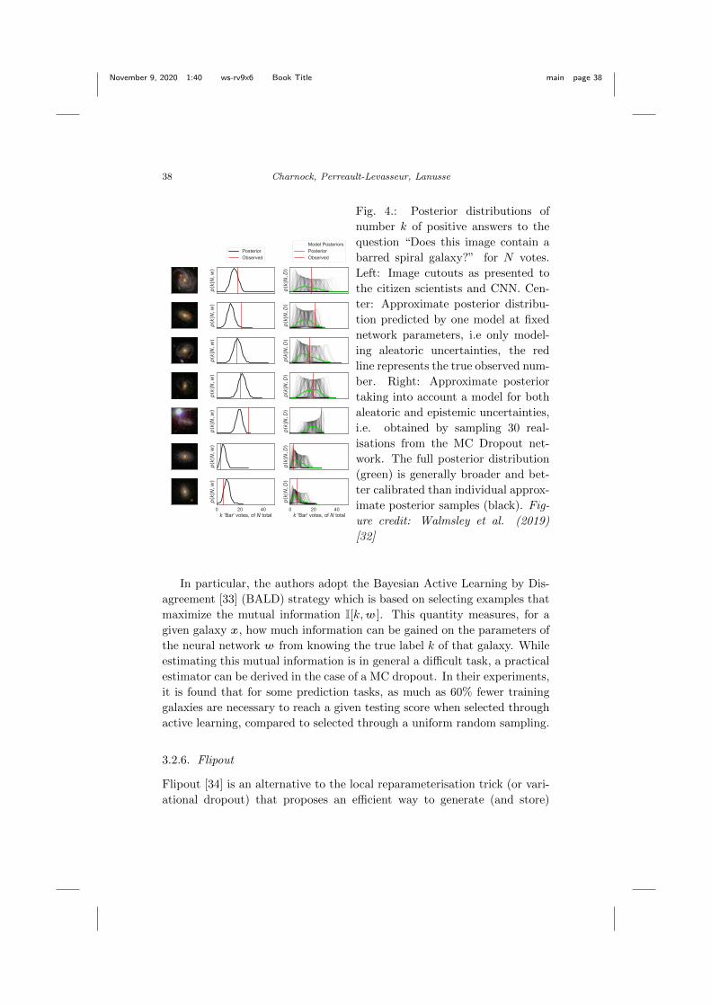
November 9, 2020 1:40 ws-rv9x6 Book Title main page 38
38 Charnock, Perreault-Levasseur, Lanusse
p(k|
N,w
)
PosteriorObserved
p(k|
N,D
)
Model PosteriorsPosteriorObserved
p(k|
N,w
)
p(k|
N,D
)
p(k|
N,w
)
p(k|
N,D
)
p(k|
N,w
)
p(k|
N,D
)
p(k|
N,w
)
p(k|
N,D
)
p(k|
N,w
)
p(k|
N,D
)
0 20 40k 'Bar' votes, of N total
p(k|
N,w
)
0 20 40k 'Bar' votes, of N total
p(k|
N,D
)
Fig. 4.: Posterior distributions of
number k of positive answers to the
question “Does this image contain a
barred spiral galaxy?” for N votes.
Left: Image cutouts as presented to
the citizen scientists and CNN. Cen-
ter: Approximate posterior distribu-
tion predicted by one model at fixed
network parameters, i.e only model-
ing aleatoric uncertainties, the red
line represents the true observed num-
ber. Right: Approximate posterior
taking into account a model for both
aleatoric and epistemic uncertainties,
i.e. obtained by sampling 30 real-
isations from the MC Dropout net-
work. The full posterior distribution
(green) is generally broader and bet-
ter calibrated than individual approx-
imate posterior samples (black). Fig-
ure credit: Walmsley et al. (2019)
[32]
In particular, the authors adopt the Bayesian Active Learning by Dis-
agreement [33] (BALD) strategy which is based on selecting examples that
maximize the mutual information I[k,w]. This quantity measures, for a
given galaxy x, how much information can be gained on the parameters of
the neural network w from knowing the true label k of that galaxy. While
estimating this mutual information is in general a difficult task, a practical
estimator can be derived in the case of a MC dropout. In their experiments,
it is found that for some prediction tasks, as much as 60% fewer training
galaxies are necessary to reach a given testing score when selected through
active learning, compared to selected through a uniform random sampling.
3.2.6. Flipout
Flipout [34] is an alternative to the local reparameterisation trick (or vari-
ational dropout) that proposes an efficient way to generate (and store)
November 9, 2020 1:40 ws-rv9x6 Book Title main page 39
Bayesian Neural Networks 39
pseudo-independent perturbations to decorrelate the gradients with respect
to parameters m = (µi,∆wi)|i ∈ [1, nw] according to each of the nelems
elements of data within a minibatch. µi and ∆wi are the mean and stochas-
tic perturbation of some network parameter w(mi). This method therefore
is more closely akin to stochastic gradient variational Bayes, where the dis-
tribution of network parameters is fitted. Note that for Flipout, the require-
ments on the distribution for each network parameter is that they are differ-
entiable with respect to the parameters m, that the distribution of pertur-
bations of the network parameters, ∆wi, is symmetric about zero (but not
necessarily Gaussian) and the network parameters are independent. With
∆wi symmetric amount zero, the multiplication by a random matrix of
signs leaves it identically distributed. This means that by choosing a single
∆wi for each network parameter (like ∆wi = σiεi for the Gaussian case)
somewhat decorrelated gradients can be obtained for each element of a mini-
batch by identically distributing ∆wi via random draws from two nelems-
length vectors, ji = jin = 2bin − 1|bin ∼ Bernoulli(0.5), n ∈ [1, nelems]and ki = kin = 2bin − 1|bin ∼ Bernoulli(0.5), n ∈ [1, nelems]. Each pa-
rameter of the network is then obtained, as with the reparameterisation
trick, via
wn(mi) = µi + ∆wijinkin. (52)
This can be performed very quickly using matrix multiplication, affording a
decrease in the variance of the stochastic gradient by a factor of ∼ 1/nelems
in comparison to using shared parameter values for an entire minibatch for
approximately twice the computational cost, although due to parallelisation
this can be done in equal time.
Example: Cosmological parameter inference and uncertainty cal-
ibration The inference of cosmological parameter values from data, such
as maps of the Cosmic Microwave Background radiation, is an important
task in these times of precision cosmology. It is therefore useful to consider
the comparison of several of the variational inference methods to calibrate
their performance [35] . The study uses two CNN architectures, AlexNet
and VGG to predict, from an image of the CMB, a Gaussian posterior dis-
tribution on a limited set of three cosmological parameters. The outputs
of these neural networks, parameterised with w, are therefore chosen to be
the mean, µ ≡ µ(x,w), and covariance, Σ ≡ Σ(x,w), of a multivariate
Gaussian distribution. The loss function used to train these networks under
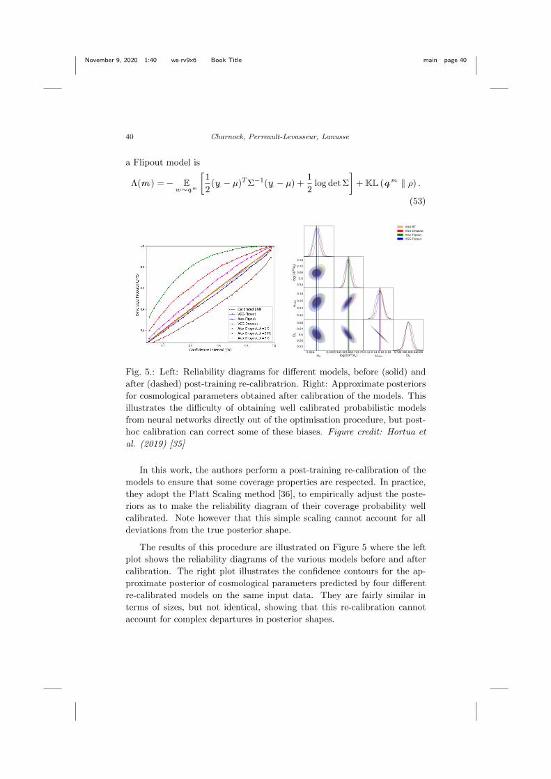
November 9, 2020 1:40 ws-rv9x6 Book Title main page 40
40 Charnock, Perreault-Levasseur, Lanusse
a Flipout model is
Λ(m) =− Ew∼qm
[1
2(y− µ)TΣ−1(y− µ) +
1
2log det Σ
]+ KL (qm ‖ ρ) .
(53)
0.520.560.600.640.68
3.54
3.6
3.66
3.72
3.78
log(
1010
A s)
0.12
0.14
0.16
0.18cd
m
0.024 0.030b
0.52
0.56
0.6
0.64
0.68
3.543.603.663.723.78log(1010As)
0.12 0.14 0.16 0.18cdm
VGG-RTVGG-DropoutAlex-FlipoutVGG-Flipout
Fig. 5.: Left: Reliability diagrams for different models, before (solid) and
after (dashed) post-training re-calibratrion. Right: Approximate posteriors
for cosmological parameters obtained after calibration of the models. This
illustrates the difficulty of obtaining well calibrated probabilistic models
from neural networks directly out of the optimisation procedure, but post-
hoc calibration can correct some of these biases. Figure credit: Hortua et
al. (2019) [35]
In this work, the authors perform a post-training re-calibration of the
models to ensure that some coverage properties are respected. In practice,
they adopt the Platt Scaling method [36], to empirically adjust the poste-
riors as to make the reliability diagram of their coverage probability well
calibrated. Note however that this simple scaling cannot account for all
deviations from the true posterior shape.
The results of this procedure are illustrated on Figure 5 where the left
plot shows the reliability diagrams of the various models before and after
calibration. The right plot illustrates the confidence contours for the ap-
proximate posterior of cosmological parameters predicted by four different
re-calibrated models on the same input data. They are fairly similar in
terms of sizes, but not identical, showing that this re-calibration cannot
account for complex departures in posterior shapes.
November 9, 2020 1:40 ws-rv9x6 Book Title main page 41
Bayesian Neural Networks 41
One of the takeaways of this work is that overall Flipout appear to
be the best performing method in terms of calibration, training speed,
and accuracy, out of the four explored (reparameterisation, Flipout, MC
Dropout, DropConnect).
3.2.7. Neutra
We can also use variational inference as part of a Markov chain sampling
scheme. Neutra [37] is a method which samples from a normal distribution
and then performs a bijective transformation, g : ε ∼ N(0, I)→ λ ∼ ρχ, to
a space approximating the target distribution. In this way it can be seen as
an approximation to the Riemannian manifold HMC (section 3.1.2) where
the metric is defined by the bijective function, I(λ) = (JJT )−1, where the
Jacobian is J= ∂εg. Using neural networks (and particularly many of the
modern density estimators such as inverse autoregressive flows, etc.) this
Jacobian is very easy to evaluate and therefore g can be arbitrarily com-
plex, fittable to the desired function by maximising the ELBO and quick
to evaluate. Using HMC, samples can be obtained very easily from the
normal distribution and the bijected forward to get samples from an ap-
proximation to the target distribution much more efficiently than samples
can be obtained by directly evaluating the target distribution. It should
be noted that this method, like all those mentioned in this section, is not
Bayesian in nature, since, in this case, there is no quantification in how
well the bijection is really performing. Therefore, there is no way to tell if
the samples, g(ε), actually coincide with samples λ ∼ ρχ, meaning the dis-
tribution could be very different from that desired when addressing target
distribution using exact evaluations.
4. Concluding Remarks and Outlook
Despite impressive accuracy in supervised learning benchmarks, current
state of the art neural networks are poor at quantifying predictive un-
certainty, and as such are prone to produce overconfident predictions and
biases which are extremely difficult to disentangle from true properties of
the data. The fact that proper uncertainty quantification is crucial for
many practical applications justifies the formulation of neural networks as
statistical models as a first step towards using them for inference.
While truly Bayesian neural networks have the capacity to fully char-
acterize the epistemic uncertainty introduced by the neural network, in
November 9, 2020 1:40 ws-rv9x6 Book Title main page 42
42 Charnock, Perreault-Levasseur, Lanusse
practice, exact Bayesian inference is intractable for neural network. It is
common to resort to either using numerically approximated by exact sam-
ples of posterior distribution of network parameters, that is, Monte Carlo
methods, or to using approximate distributions as a proxy for the true
Bayesian posterior, through variational inference. The fact that, through
the former method, Bayesian neural networks are often harder to train and
implement than non-Bayesian neural networks means that, in the litera-
ture, variational methods have gained a lot of popularity in the recent years.
However, as we have have stressed in this chapter, those latter approximate
methods suffer from many pitfalls, in particular the lack of guarantee that
the approximate distribution is sufficiently close to the desired target.
Because of these, other statistical tools and tests should be used in con-
currence with approximate Bayesian neural networks, such as calibration
and test of generalization of the predictive uncertainty to domain shifts [38].
However, it is worth noting that Bayesian neural networks are not neces-
sarily the most useful for doing the best reasoned inference of network out-
puts. For this, other methods, such as likelihood-free (simulation-based)
inference, could be more efficient, powerful, and easier to implement.
References
[1] K. Athreya and S. Lahiri, Measure Theory and Probability Theory. SpringerTexts in Statistics, Springer (2006). ISBN 9780387329031.
[2] P. Muller and D. Rios, Issues in bayesian analysis of neural network models,Neural computation. 10, 749–70 (03, 1998).
[3] T. Charnock, G. Lavaux, B. D. Wandelt, S. Sarma Boruah, J. Jasche, andM. J. Hudson, Neural physical engines for inferring the halo mass distribu-tion function, Monthly Notices of the Royal Astronomical Society. 494(1),50–61 (Mar., 2020). doi: 10.1093/mnras/staa682.
[4] D. Hafner, D. Tran, T. Lillicrap, A. Irpan, and J. Davidson, Noise Con-trastive Priors for Functional Uncertainty (2018). URL http://arxiv.org/
abs/1807.09289.[5] B. Lakshminarayanan, A. Pritzel, and C. Blundell. Simple and scalable pre-
dictive uncertainty estimation using deep ensembles. In eds. I. Guyon, U. V.Luxburg, S. Bengio, H. Wallach, R. Fergus, S. Vishwanathan, and R. Gar-nett, Advances in Neural Information Processing Systems 30, pp. 6402–6413.Curran Associates, Inc. (2017).
[6] E. A. J. F. Peters and G. de With, Rejection-free monte carlo sam-pling for general potentials, Phys. Rev. E. 85, 026703 (Feb, 2012). doi:10.1103/PhysRevE.85.026703. URL https://link.aps.org/doi/10.1103/
PhysRevE.85.026703.[7] A. Bouchard-Cote, S. Vollmer, and A. Doucet, The bouncy particle sampler:
November 9, 2020 1:40 ws-rv9x6 Book Title main page 43
Bayesian Neural Networks 43
a non-reversible rejection-free Markov chain Monte Carlo method (2015).Technical report arxiv:1510.02451.
[8] A. Beskos, N. S. Pillai, G. O. Roberts, J. M. Sanz-Serna, and A. M. Stuart.Optimal tuning of the hybrid monte-carlo algorithm (2010).
[9] Y. Bouffanais and E. K. Porter, Bayesian inference for binary neutronstar inspirals using a hamiltonian monte carlo algorithm, Phys. Rev. D.100, 104023 (Nov, 2019). doi: 10.1103/PhysRevD.100.104023. URL https:
//link.aps.org/doi/10.1103/PhysRevD.100.104023.[10] M. D. Hoffman and A. Gelman, The No-U-Turn Sampler : Adaptively Set-
ting Path Lengths in Hamiltonian Monte Carlo. 15, 1351–1381 (2014).[11] X. Lu, V. Perrone, L. Hasenclever, Y. W. Teh, and S. J. Vollmer, Relativistic
Monte Carlo, Proceedings of the 20th International Conference on ArtificialIntelligence and Statistics, AISTATS 2017. (1), 1–11 (2017).
[12] T. Fu and Z. Zhang. Quasi-Newton Hamiltonian Monte Carlo. In Conferenceon Uncertainty in Artificial Intelligence (UAI) (2016).
[13] J. Jasche and B. D. Wandelt, Bayesian physical reconstruction of initialconditions from large-scale structure surveys, Monthly Notices of the RoyalAstronomical Society. 432(2), 894–913 (Jun, 2013). doi: 10.1093/mnras/stt449.
[14] J. Jasche, F. Leclercq, and B. D. Wandelt, Past and present cosmic structurein the SDSS DR7 main sample, Journal of Cosmology and AstroparticlePhysics. 2015(1):036 (Jan, 2015). doi: 10.1088/1475-7516/2015/01/036.
[15] G. Lavaux and J. Jasche, Unmasking the masked Universe: the 2M++catalogue through Bayesian eyes, Monthly Notices of the Royal AstronomicalSociety. 455(3), 3169–3179 (Jan, 2016). doi: 10.1093/mnras/stv2499.
[16] D. Kodi Ramanah, T. Charnock, and G. Lavaux, Painting halos from cosmicdensity fields of dark matter with physically motivated neural networks,Physical Review D. 100(4):043515 (Aug., 2019). doi: 10.1103/PhysRevD.100.043515.
[17] M. Girolami, B. Calderhead, and S. A. Chin, Riemannian Manifold Hamil-tonian Monte Carlo (2009). URL http://arxiv.org/abs/0907.1100.
[18] T. Chen, E. B. Fox, and C. Guestrin. Stochastic gradient Hamiltonian MonteCarlo. In 31st International Conference on Machine Learning, ICML 2014,vol. 5, pp. 3663–3676 (feb, 2014). ISBN 9781634393973. URL http://arxiv.
org/abs/1402.4102.[19] C. Blundell, J. Cornebise, K. Kavukcuoglu, and D. Wierstra, Weight Un-
certainty in Neural Networks, arXiv e-prints. p. arXiv:1505.05424 (5, 2015).URL http://arxiv.org/abs/1505.05424.
[20] G. Dikov, P. van der Smagt, and J. Bayer, Bayesian Learning of NeuralNetwork Architectures (1, 2019). URL http://arxiv.org/abs/1901.04436.
[21] D. P. Kingma, Fast Gradient-Based Inference with Continuous Latent Vari-able Models in Auxiliary Form, arXiv e-prints. art. arXiv:1306.0733 (June,2013).
[22] D. P. Kingma and M. Welling, Auto-Encoding Variational Bayes, arXiv e-prints. art. arXiv:1312.6114 (Dec., 2013).
[23] A. Moller and T. de Boissiere, SuperNNova: an open-source framework
November 9, 2020 1:40 ws-rv9x6 Book Title main page 44
44 Charnock, Perreault-Levasseur, Lanusse
for Bayesian, neural network-based supernova classification, Monthly No-tices of the Royal Astronomical Society. 491(3), 4277–4293 (1, 2020). ISSN0035-8711. doi: 10.1093/mnras/stz3312. URL https://academic.oup.com/
mnras/article/491/3/4277/5651173.[24] M. Fortunato, C. Blundell, and O. Vinyals, Bayesian Recurrent Neural Net-
works. pp. 1–14 (apr, 2017). URL http://arxiv.org/abs/1704.02798.[25] M. H. DeGroot and S. E. Fienberg, The Comparison and Evaluation of Fore-
casters, Journal of the Royal Statistical Society. Series D (The Statistician).32(1/2), 12–22 (1983). ISSN 00390526, 14679884. URL http://www.jstor.
org/stable/2987588.[26] D. P. Kingma, T. Salimans, and M. Welling. Variational Dropout and the
Local Reparameterization Trick. Technical report .[27] Y. Gal and Z. Ghahramani, Dropout as a Bayesian Approximation:
Representing Model Uncertainty in Deep Learning, arXiv e-prints. p.arXiv:1506.02142 (6, 2015). URL http://arxiv.org/abs/1506.02142.
[28] Y. Gal, J. Hron, and A. Kendall, Concrete Dropout, arXiv e-prints. p.arXiv:1705.07832 (5, 2017).
[29] G. E. Hinton, N. Srivastava, A. Krizhevsky, I. Sutskever, and R. Salakhutdi-nov, Improving neural networks by preventing co-adaptation of feature de-tectors, CoRR. abs/1207.0580 (2012). URL http://arxiv.org/abs/1207.
0580.[30] R. Houthooft, X. Chen, Y. Duan, J. Schulman, F. De Turck, and P. Abbeel,
VIME: Variational Information Maximizing Exploration (5, 2016). URLhttp://arxiv.org/abs/1605.09674.
[31] L. Perreault Levasseur, Y. D. Hezaveh, and R. H. Wechsler, Uncertainties inParameters Estimated with Neural Networks: Application to Strong Gravi-tational Lensing, The Astrophysical Journal. 850(1), L7 (11, 2017). ISSN2041-8213.doi: 10.3847/2041-8213/aa9704. URL http://stacks.iop.org/2041-8205/
850/i=1/a=L7?key=crossref.dd8f01b687a77b74ce33239cdb39c453.[32] M. Walmsley, L. Smith, C. Lintott, Y. Gal, S. Bamford, H. Dickinson,
L. Fortson, S. Kruk, K. Masters, C. Scarlata, B. Simmons, R. Smethurst, andD. Wright, Galaxy Zoo: probabilistic morphology through Bayesian CNNsand active learning, Monthly Notices of the Royal Astronomical Society. 491(2), 1554–1574 (1, 2020). ISSN 0035-8711. doi: 10.1093/mnras/stz2816. URLhttps://academic.oup.com/mnras/article/491/2/1554/5583078.
[33] D. J. C. MacKay, Information-Based Objective Functions for Active DataSelection, Neural Computation. 4(4), 590–604 (1992). ISSN 0899-7667. doi:10.1162/neco.1992.4.4.590.
[34] Y. Wen, P. Vicol, J. Ba, D. Tran, and R. Grosse, Flipout: Efficient pseudo-independent weight perturbations on mini-batches, 6th International Con-ference on Learning Representations, ICLR 2018 - Conference Track Pro-ceedings. pp. 1–16 (2018).
[35] H. J. Hortua, R. Volpi, D. Marinelli, and L. Malago, Parameters Estima-tion for the Cosmic Microwave Background with Bayesian Neural Networks,arXiv e-prints. p. arXiv:1911.08508 (11, 2019).
November 9, 2020 1:40 ws-rv9x6 Book Title main page 45
Bayesian Neural Networks 45
[36] M. Kull, T. d. M. e Silva Filho, and P. Flach, Beta calibration: A well-founded and easily implemented improvement on logistic calibration for bi-nary classifiers, Proceedings of the 20th International Conference on Artifi-cial Intelligence and Statistics, AISTATS 2017. 54 (2017).
[37] M. Hoffman, P. Sountsov, J. V. Dillon, I. Langmore, D. Tran, and S. Va-sudevan, NeuTra-lizing Bad Geometry in Hamiltonian Monte Carlo UsingNeural Transport, arXiv e-prints. art. arXiv:1903.03704 (Mar., 2019).
[38] J. Snoek, Y. Ovadia, E. Fertig, B. Lakshminarayanan, S. Nowozin, D. Scul-ley, J. Dillon, J. Ren, and Z. Nado. Can you trust your model’s uncertainty?evaluating predictive uncertainty under dataset shift. In eds. H. Wallach,H. Larochelle, A. Beygelzimer, F. d’Alche Buc, E. Fox, and R. Garnett,Advances in Neural Information Processing Systems 32, pp. 13991–14002.Curran Associates, Inc. (2019).