Chapter 1 Classical Scattering Theory - College of Charlestonwilliamsgj.people.cofc.edu/Scattering Theory.pdfChapter 1 Classical Scattering Theory 1.1 Relative Motion of Projectile

Chapter 1Classical Scattering Theory

1.1 Relative Motion of Projectile and Target

Consider two particles, projectile and target, with masses m1 and m2 respectively,which interact via a time-independent potential V depending on the separation

r = r1 − r2 (1.1)

of their position vectors r1 and r2. In the absence of external forces, the centre ofmass Rcm = (m1r1 +m2r2)/(m1 +m2) moves uniformly, Rcm(t) = Rcm(0)+Vcmt .In the centre-of-mass frame of reference, that is the inertial system in which thecentre of mass of the two particles is at rest, the position vectors of the two particlesare

r(cm)1 = m2

m1 + m2r, r(cm)

2 = − m1

m1 + m2r. (1.2)

Scattering experiments in the laboratory usually involve a projectile initially movingfreely towards a target at rest,

r(in, lab)1 (t) = r(in, lab)

1 (0) + v(in, lab)1 t, r(in, lab)

2 (t) = r(in, lab)2 (0), (1.3)

so the centre-of-mass velocity in the laboratory frame of reference is simply V(lab)cm =

r(in, lab)1 m1/(m1 + m2).

Throughout this book we shall focus on the relative motion of projectile andtarget, which contains the essential nontrivial physics of the scattering problem. Therelevant coordinate is the relative distance (1.1). Transformation to the laboratoryframe of reference is achieved via (1.2) and r(lab)

i (t) = r(cm)i (t) + R(lab)

cm (t), i = 1,2.Details of such straightforward but nontrivial transformations are discussed, e.g., inparagraph 17 of [2].

Classically, the evolution of r(t) is described by Newton’s equation of motion

μr = −∇V (r), μ = m1m2

m1 + m2, (1.4)

as for one particle with the reduced mass μ moving under the influence of the po-tential V (r). In accordance with standard convention, we assume the asymptotic in-coming velocity v∞ = limt→−∞ r(t) to point in the direction of the positive z-axis,

H. Friedrich, Scattering Theory, Lecture Notes in Physics 872,DOI 10.1007/978-3-642-38282-6_1, © Springer-Verlag Berlin Heidelberg 2013

1

http://dx.doi.org/10.1007/978-3-642-38282-6_1

2 1 Classical Scattering Theory

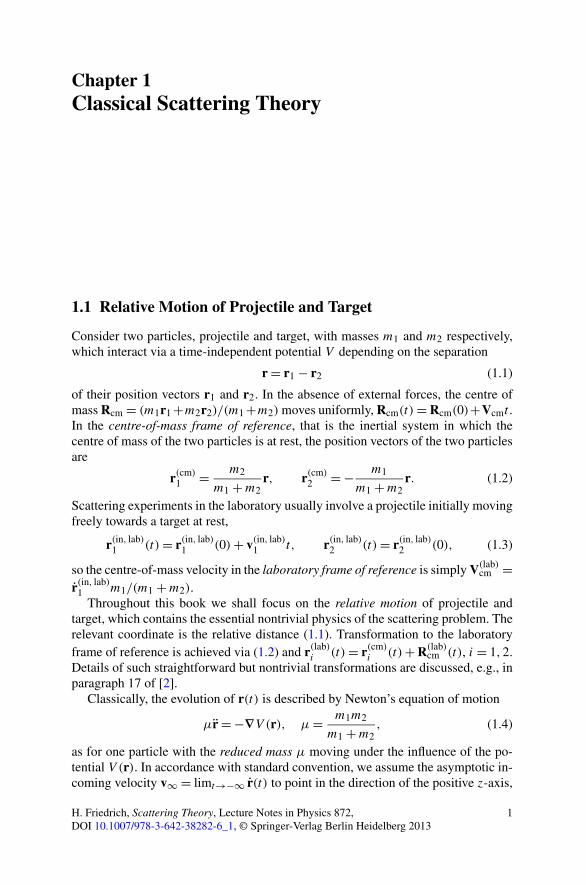
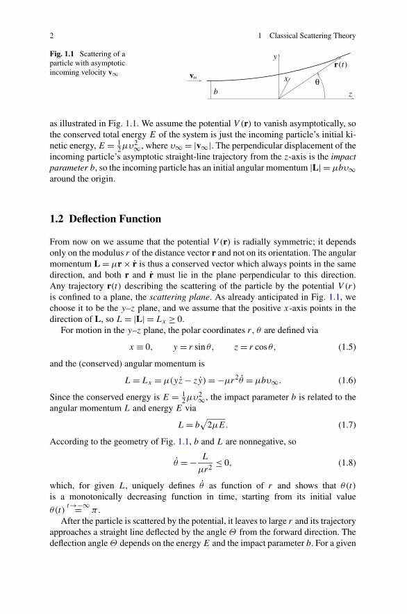
Fig. 1.1 Scattering of aparticle with asymptoticincoming velocity v∞

as illustrated in Fig. 1.1. We assume the potential V (r) to vanish asymptotically, sothe conserved total energy E of the system is just the incoming particle’s initial ki-netic energy, E = 1

2μυ2∞, where υ∞ = |v∞|. The perpendicular displacement of theincoming particle’s asymptotic straight-line trajectory from the z-axis is the impactparameter b, so the incoming particle has an initial angular momentum |L| = μbυ∞around the origin.

1.2 Deflection Function

From now on we assume that the potential V (r) is radially symmetric; it dependsonly on the modulus r of the distance vector r and not on its orientation. The angularmomentum L = μr × r is thus a conserved vector which always points in the samedirection, and both r and r must lie in the plane perpendicular to this direction.Any trajectory r(t) describing the scattering of the particle by the potential V (r)

is confined to a plane, the scattering plane. As already anticipated in Fig. 1.1, wechoose it to be the y–z plane, and we assume that the positive x-axis points in thedirection of L, so L = |L| = Lx ≥ 0.

For motion in the y–z plane, the polar coordinates r , θ are defined via

x ≡ 0, y = r sin θ, z = r cos θ, (1.5)

and the (conserved) angular momentum is

L = Lx = μ(yz − zy) = −μr2θ = μbυ∞. (1.6)

Since the conserved energy is E = 12μυ2∞, the impact parameter b is related to the

angular momentum L and energy E via

L = b√

2μE. (1.7)

According to the geometry of Fig. 1.1, b and L are nonnegative, so

θ = − L

μr2≤ 0, (1.8)

which, for given L, uniquely defines θ as function of r and shows that θ(t)

is a monotonically decreasing function in time, starting from its initial value

θ(t)t→−∞= π .

After the particle is scattered by the potential, it leaves to large r and its trajectoryapproaches a straight line deflected by the angle Θ from the forward direction. Thedeflection angle Θ depends on the energy E and the impact parameter b. For a given

1.2 Deflection Function 3

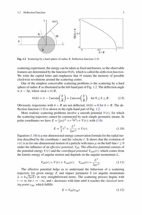
Fig. 1.2 Scattering by a hard sphere of radius R. Deflection function (1.9)

scattering experiment, the energy can be taken as fixed and known, so the observablefeatures are determined by the function Θ(b), which is called the deflection function.We write the capital letter and emphasize that Θ retains the memory of possibleclockwise revolutions around the scattering centre.

One of the simplest conceivable scattering problems is the scattering by a hardsphere of radius R as illustrated in the left-hand part of Fig. 1.2. The deflection angleis π − 2φ, where sinφ = b/R,

Θ(b) = π − 2 arcsin

(b

R

)= 2 arccos

(b

R

)for 0 ≤ b ≤ R. (1.9)

Obviously, trajectories with b > R are not deflected, Θ(b) = 0 for b > R. The de-flection function (1.9) is shown in the right-hand part of Fig. 1.2.

More realistic scattering problems involve a smooth potential V (r), for whichthe scattering trajectory cannot be constructed by such simple geometric means. Inpolar coordinates we have E = 1

2μ(r2 + r 2θ2) + V (r); with (1.8):

E = μ

2r2 + L2

2μr2+ V (r). (1.10)

Equation (1.10) is a one-dimensional energy-conservation formula for the radial mo-tion described by the coordinate r and the velocity r . It shows that the evolution ofr(t) is as for one-dimensional motion of a particle with mass μ on the half-line r ≥ 0under the influence of an effective potential, Veff. The effective potential consists ofthe potential energy V (r) and the centrifugal potential Vcent(r), which comes fromthe kinetic energy of angular motion and depends on the angular momentum L,

Veff(r) = V (r) + Vcent(r), Vcent(r) = L2

2μr2. (1.11)

The effective potential helps us to understand the behaviour of a scatteringtrajectory for given energy E and impact parameter b (or angular momentumL = b

√2μE) in very straightforward terms. The scattering process begins with

r → ∞ for t → −∞, and r decreases with time until it reaches the classical turn-ing point rctp, which fulfills

E = Veff(rctp) (1.12)


and corresponds to the point of closest approach of target and projectile. For thehard-sphere case in Fig. 1.2, rctp is the sphere’s radius R as long as b ≤ R. IfVeff(r) < E for all r , then the radial turning point is the origin, rctp = 0. It is a usefulconvention to choose the time of closest approach to be t = 0: r(t = 0) = rctp. Forlater (positive) times, r increases again until r → ∞ for t → +∞.

The trajectory of the particle in the y–z-plane is most conveniently obtained viadθ/dr = θ/r with θ from (1.8) and r = ±√

(2/μ)[E − Veff(r)] from (1.10),

dθ

dr= ± L

r2√

2μ[E − Veff(r)] . (1.13)

During the first half of the scattering process, r is negative (as is θ ), so the plus signon the right-hand side of (1.13) applies. During the second half, r is positive (incontrast to θ ), so (1.13) applies with the minus sign. The polar angle of the point ofclosest approach, for which r = rctp, is

θ(r = rctp) = π +∫ rctp

∞dθ

drdr = π −

∫ ∞

rctp

L dr

r2√

2μ[E − Veff(r)] . (1.14)

For an actual calculation, the scattering trajectory (r, θ) in the y–z plane can beobtained via

θ(r) = θ(r = rctp) ±∫ r

rctp

L dr ′

r ′2√2μ[E − Veff(r ′)] , (1.15)

where the plus sign gives the points on the incoming half of the trajectory and theminus sign the points on the outgoing half. The deflection function follows from theexpression (1.15) for the polar angle in the limit r → ∞ on the outgoing branch ofthe trajectory,

Θ(b) = θ(rctp) −∫ ∞

rctp

L dr

r2√

2μ[E − Veff(r)] = π −∫ ∞

rctp

2L dr

r2√

2μ[E − Veff(r)]

= π −∫ ∞

rctp

2b

r2

[1 − b2

r2− V (r)

E

]−1/2

dr. (1.16)

In the limit of large impact parameters, the effective potential (1.11) is dominatedby the centrifugal term and the deflection angle tends to zero. For a potential fallingoff asymptotically as an inverse power of r ,

V (r)r→∞∼ Cα

rα, α > 0, (1.17)

the large-b behaviour of Θ(b) is easily calculated analytically. Changing the inte-gration variable in (1.16) from r to ξ = r/rctp gives, for large b,

Θ(b) = π −∫ ∞

1

2 dξ√

ξ4 − ξ2 + ε(ξ4 − ξ4−α), where ε =

(rctp

b

)2

− 1. (1.18)

Expanding the integrand in terms of the small parameter εb→∞∼ Cα/(E bα) yields

Θ(b)b→∞∼ Cα

E bα

πΓ (α)

2α−1[Γ (α2 )]2

= Cα

Ebα

√πΓ (α+1

2 )

Γ (α2 )

. (1.19)


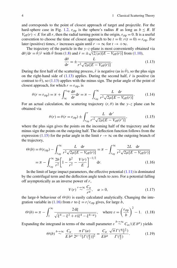
Fig. 1.3 Effective potential (1.21) for a repulsive (C > 0, left-hand part) and an attractive (C < 0,right-hand part) Kepler–Coulomb interaction. The dotted lines show the respective potential (1.20)without centrifugal contribution

1.2.1 Kepler–Coulomb Potential

The Kepler or Coulomb potential,

V (r) = C

r, (1.20)

is important, because it describes gravitational and electrostatic interactions. Forsuch a homogeneous potential of degree −1, the solutions of Newton’s equation ofmotion (1.4) obey a simple scaling relation called Kepler’s third law. If r(t) is asolution at energy E, then sr(s3/2t) is a solution at energy E/s, see Appendix A.1.The geometric shape of a trajectory does not depend on the potential strength coef-ficient C, the impact parameter b and the energy E independently, but only on theratio of C to the product Eb.

The weight of the centrifugal contribution in the effective potential (1.11) can beexpressed via the length parameter

rL = L2

μ|C| , so Veff(r) = |C|2rL

[±2

rL

r+

(rL

r

)2]. (1.21)

In the repulsive case, C > 0, the plus sign in the square bracket applies; the effectivepotential is a monotonically decreasing function of r . In the attractive case, C < 0,Veff(r) has a zero at rL/2 and a minimum at rL with Veff(rL) = −|C|/(2rL). Theeffective potential (1.21) is shown for both the repulsive and the attractive case inFig. 1.3.

The classical turning point is

rctp = b(√

γ 2 + 1 ± γ)

with γ = |C|2Eb

, (1.22)


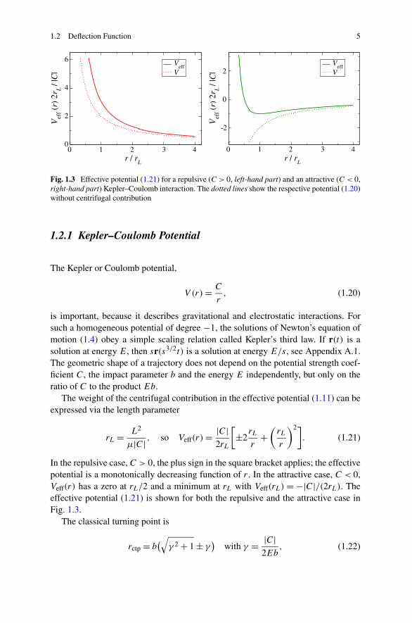
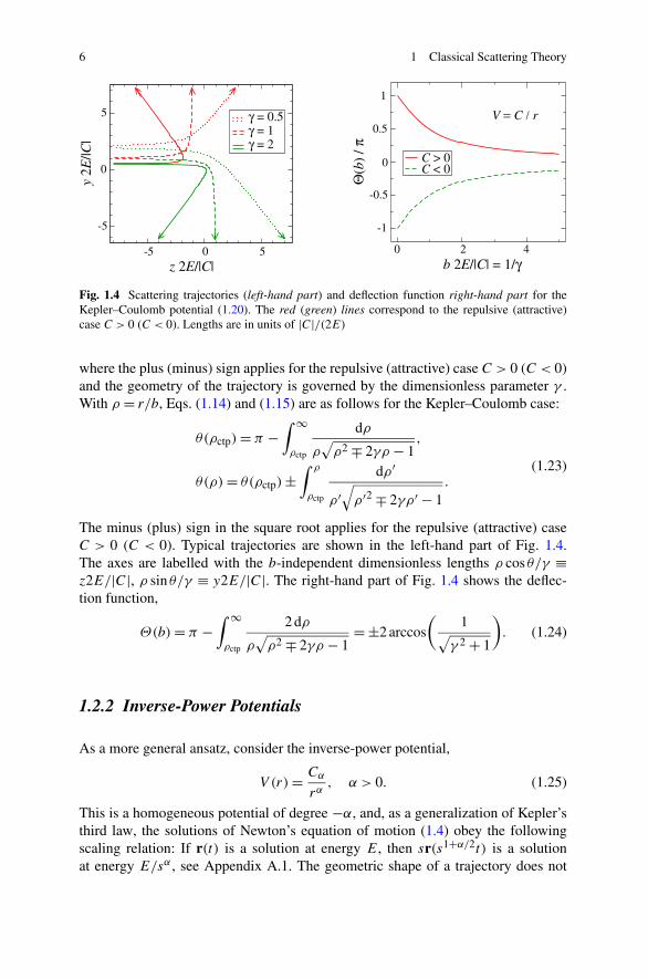
Fig. 1.4 Scattering trajectories (left-hand part) and deflection function right-hand part for theKepler–Coulomb potential (1.20). The red (green) lines correspond to the repulsive (attractive)case C > 0 (C < 0). Lengths are in units of |C|/(2E)

where the plus (minus) sign applies for the repulsive (attractive) case C > 0 (C < 0)and the geometry of the trajectory is governed by the dimensionless parameter γ .With ρ = r/b, Eqs. (1.14) and (1.15) are as follows for the Kepler–Coulomb case:

θ(ρctp) = π −∫ ∞

ρctp

dρ

ρ√

ρ2 ∓ 2γρ − 1,

θ(ρ) = θ(ρctp) ±∫ ρ

ρctp

dρ′

ρ′√

ρ′2 ∓ 2γρ′ − 1.

(1.23)

The minus (plus) sign in the square root applies for the repulsive (attractive) caseC > 0 (C < 0). Typical trajectories are shown in the left-hand part of Fig. 1.4.The axes are labelled with the b-independent dimensionless lengths ρ cos θ/γ ≡z2E/|C|, ρ sin θ/γ ≡ y2E/|C|. The right-hand part of Fig. 1.4 shows the deflec-tion function,

Θ(b) = π −∫ ∞

ρctp

2 dρ

ρ√

ρ2 ∓ 2γρ − 1= ±2 arccos

(1

√γ 2 + 1

). (1.24)

1.2.2 Inverse-Power Potentials

As a more general ansatz, consider the inverse-power potential,

V (r) = Cα

rα, α > 0. (1.25)

This is a homogeneous potential of degree −α, and, as a generalization of Kepler’sthird law, the solutions of Newton’s equation of motion (1.4) obey the followingscaling relation: If r(t) is a solution at energy E, then sr(s1+α/2t) is a solutionat energy E/sα , see Appendix A.1. The geometric shape of a trajectory does not


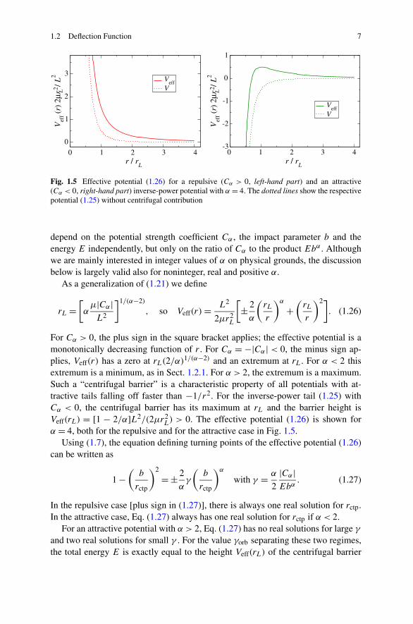
Fig. 1.5 Effective potential (1.26) for a repulsive (Cα > 0, left-hand part) and an attractive(Cα < 0, right-hand part) inverse-power potential with α = 4. The dotted lines show the respectivepotential (1.25) without centrifugal contribution

depend on the potential strength coefficient Cα , the impact parameter b and theenergy E independently, but only on the ratio of Cα to the product Ebα . Althoughwe are mainly interested in integer values of α on physical grounds, the discussionbelow is largely valid also for noninteger, real and positive α.

As a generalization of (1.21) we define

rL =[α

μ|Cα|L2

]1/(α−2)

, so Veff(r) = L2

2μr2L

[± 2

α

(rL

r

)α

+(

rL

r

)2]. (1.26)

For Cα > 0, the plus sign in the square bracket applies; the effective potential is amonotonically decreasing function of r . For Cα = −|Cα| < 0, the minus sign ap-plies, Veff(r) has a zero at rL(2/α)1/(α−2) and an extremum at rL. For α < 2 thisextremum is a minimum, as in Sect. 1.2.1. For α > 2, the extremum is a maximum.Such a “centrifugal barrier” is a characteristic property of all potentials with at-tractive tails falling off faster than −1/r2. For the inverse-power tail (1.25) withCα < 0, the centrifugal barrier has its maximum at rL and the barrier height isVeff(rL) = [1 − 2/α]L2/(2μr2

L) > 0. The effective potential (1.26) is shown forα = 4, both for the repulsive and for the attractive case in Fig. 1.5.

Using (1.7), the equation defining turning points of the effective potential (1.26)can be written as

1 −(

b

rctp

)2

= ± 2

αγ

(b

rctp

)α

with γ = α

2

|Cα|Ebα

. (1.27)

In the repulsive case [plus sign in (1.27)], there is always one real solution for rctp.In the attractive case, Eq. (1.27) always has one real solution for rctp if α < 2.

For an attractive potential with α > 2, Eq. (1.27) has no real solutions for large γ

and two real solutions for small γ . For the value γorb separating these two regimes,the total energy E is exactly equal to the height Veff(rL) of the centrifugal barrier


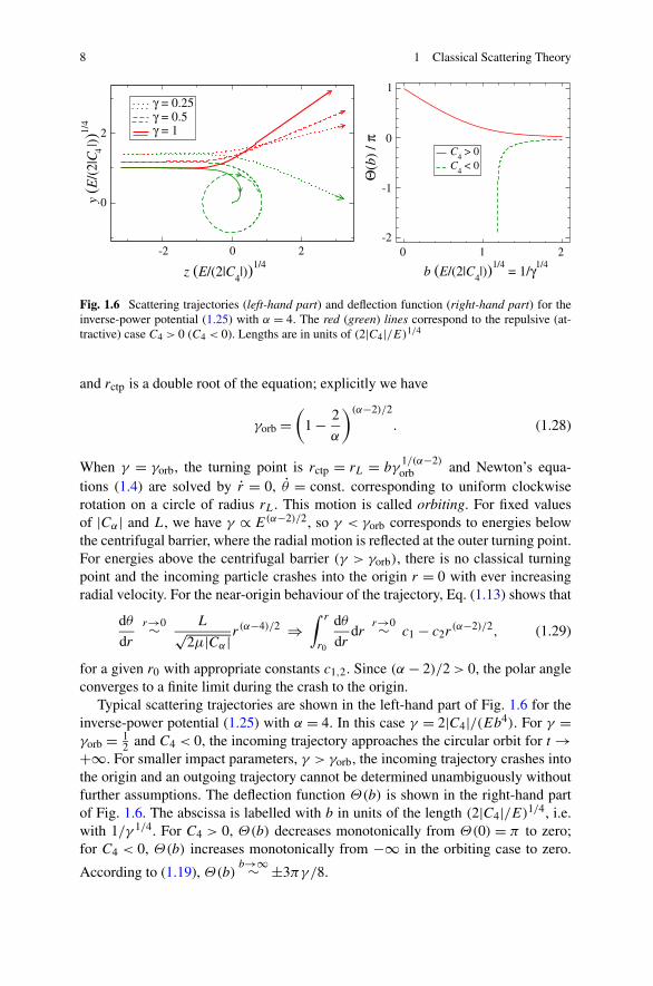
Fig. 1.6 Scattering trajectories (left-hand part) and deflection function (right-hand part) for theinverse-power potential (1.25) with α = 4. The red (green) lines correspond to the repulsive (at-tractive) case C4 > 0 (C4 < 0). Lengths are in units of (2|C4|/E)1/4

and rctp is a double root of the equation; explicitly we have

γorb =(

1 − 2

α

)(α−2)/2

. (1.28)

When γ = γorb, the turning point is rctp = rL = bγ1/(α−2)

orb and Newton’s equa-tions (1.4) are solved by r = 0, θ = const. corresponding to uniform clockwiserotation on a circle of radius rL. This motion is called orbiting. For fixed valuesof |Cα| and L, we have γ ∝ E(α−2)/2, so γ < γorb corresponds to energies belowthe centrifugal barrier, where the radial motion is reflected at the outer turning point.For energies above the centrifugal barrier (γ > γorb), there is no classical turningpoint and the incoming particle crashes into the origin r = 0 with ever increasingradial velocity. For the near-origin behaviour of the trajectory, Eq. (1.13) shows that

dθ

dr

r→0∼ L√2μ|Cα| r

(α−4)/2 ⇒∫ r

r0

dθ

drdr

r→0∼ c1 − c2r(α−2)/2, (1.29)

for a given r0 with appropriate constants c1,2. Since (α − 2)/2 > 0, the polar angleconverges to a finite limit during the crash to the origin.

Typical scattering trajectories are shown in the left-hand part of Fig. 1.6 for theinverse-power potential (1.25) with α = 4. In this case γ = 2|C4|/(Eb4). For γ =γorb = 1

2 and C4 < 0, the incoming trajectory approaches the circular orbit for t →+∞. For smaller impact parameters, γ > γorb, the incoming trajectory crashes intothe origin and an outgoing trajectory cannot be determined unambiguously withoutfurther assumptions. The deflection function Θ(b) is shown in the right-hand partof Fig. 1.6. The abscissa is labelled with b in units of the length (2|C4|/E)1/4, i.e.with 1/γ 1/4. For C4 > 0, Θ(b) decreases monotonically from Θ(0) = π to zero;for C4 < 0, Θ(b) increases monotonically from −∞ in the orbiting case to zero.

According to (1.19), Θ(b)b→∞∼ ±3πγ/8.


Scattering by attractive inverse-power potentials (1.25) depends crucially onwhether the power α is larger or smaller than two, i.e. if there is a centrifugal barrieror not. The boundary separating these two regimes is provided by inverse-squarepotentials

V (r) = C2

r2, Veff(r) = L2

2μr2, L2 = L2 + 2μC2. (1.30)

As long as L2 is greater than zero, the deflection function can be calculated in a verystraightforward way. Since Θ(b) is identically zero for a free particle, the integralon the far right of the upper line of Eq. (1.16) must be equal to π . This also holdsfor the effective potential (1.30), if we replace the true angular momentum L in the

numerator of the integrand by L =√

L2, so

Θ(b) = π

(1 − L

L

). (1.31)

If L2 ≤ 0, the effective potential (1.30) has no turning point and the scattering trajec-

tory crashes into the origin. For L2 < 0, dθ/drr→0∝ 1/r according to (1.29), whereas

dθ/drr→0∝ 1/r2 for L2 = 0; in both cases the particle encircles the origin infinitely

many times during the crash.

1.2.3 Lennard–Jones Potential

Realistic potentials have more structure than the inverse-power potentials discussedabove. For example, the interaction of two neutral atoms with each other is char-acterized at large distances by an attractive tail proportional to −1/r6, and it isstrongly repulsive at very short distances comparable to the size of the atoms. A pop-ular model for describing interatomic interactions is the Lennard–Jones potential,

VLJ(r) = C12

r12− C6

r6= E

[(rmin

r

)12

− 2

(rmin

r

)6]. (1.32)

It has a minimum at rmin = (2C12/C6)1/6, and VLJ(rmin) = −E = −C6

2/(4C12).We express the angular momentum in terms of a dimensionless quantity Λ,

Λ = L

rmin√

2μE, so Veff = E

[(rmin

r

)12

− 2

(rmin

r

)6

+ Λ2(

rmin

r

)2].

(1.33)

Λ2 is the ratio of the centrifugal potential at rmin to the depth E of the poten-tial (1.32). Figure 1.7 shows the effective potential (1.33) for Λ2 = 0,1,2 and 3.Note that Veff(r) only has a local maximum if the angular momentum is less than alimiting value, Λ < Λorb. For Λ = Λorb, Veff has a horizontal point of inflection atrorb. From V ′

eff(rorb) = 0 and V ′′eff(rorb) = 0 we get


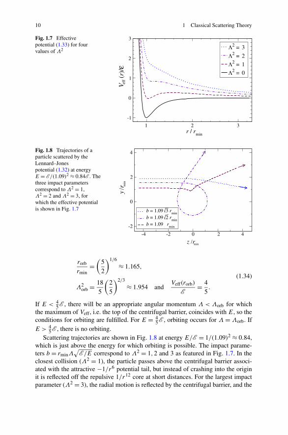
Fig. 1.7 Effectivepotential (1.33) for fourvalues of Λ2

Fig. 1.8 Trajectories of aparticle scattered by theLennard–Jonespotential (1.32) at energyE = E /(1.09)2 ≈ 0.84E . Thethree impact parameterscorrespond to Λ2 = 1,Λ2 = 2 and Λ2 = 3, forwhich the effective potentialis shown in Fig. 1.7

rorb

rmin=

(5

2

)1/6

≈ 1.165,

Λ2orb = 18

5

(2

5

)2/3

≈ 1.954 andVeff(rorb)

E= 4

5.

(1.34)

If E < 45E , there will be an appropriate angular momentum Λ < Λorb for which

the maximum of Veff, i.e. the top of the centrifugal barrier, coincides with E, so theconditions for orbiting are fulfilled. For E = 4

5E , orbiting occurs for Λ = Λorb. IfE > 4

5E , there is no orbiting.Scattering trajectories are shown in Fig. 1.8 at energy E/E = 1/(1.09)2 ≈ 0.84,

which is just above the energy for which orbiting is possible. The impact parame-ters b = rminΛ

√E /E correspond to Λ2 = 1,2 and 3 as featured in Fig. 1.7. In the

closest collision (Λ2 = 1), the particle passes above the centrifugal barrier associ-ated with the attractive −1/r6 potential tail, but instead of crashing into the originit is reflected off the repulsive 1/r12 core at short distances. For the largest impactparameter (Λ2 = 3), the radial motion is reflected by the centrifugal barrier, and the

1.3 Scattering Angle and Scattering Cross Sections 11

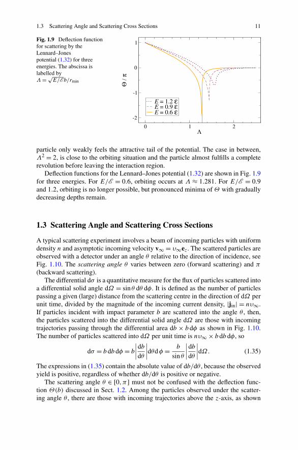
Fig. 1.9 Deflection functionfor scattering by theLennard–Jonespotential (1.32) for threeenergies. The abscissa islabelled byΛ = √

E/E b/rmin

particle only weakly feels the attractive tail of the potential. The case in between,Λ2 = 2, is close to the orbiting situation and the particle almost fulfills a completerevolution before leaving the interaction region.

Deflection functions for the Lennard–Jones potential (1.32) are shown in Fig. 1.9for three energies. For E/E = 0.6, orbiting occurs at Λ ≈ 1.281. For E/E = 0.9and 1.2, orbiting is no longer possible, but pronounced minima of Θ with graduallydecreasing depths remain.

1.3 Scattering Angle and Scattering Cross Sections

A typical scattering experiment involves a beam of incoming particles with uniformdensity n and asymptotic incoming velocity v∞ = υ∞ez. The scattered particles areobserved with a detector under an angle θ relative to the direction of incidence, seeFig. 1.10. The scattering angle θ varies between zero (forward scattering) and π

(backward scattering).The differential dσ is a quantitative measure for the flux of particles scattered into

a differential solid angle dΩ = sin θ dθ dφ. It is defined as the number of particlespassing a given (large) distance from the scattering centre in the direction of dΩ perunit time, divided by the magnitude of the incoming current density, |jin| = nυ∞.If particles incident with impact parameter b are scattered into the angle θ , then,the particles scattered into the differential solid angle dΩ are those with incomingtrajectories passing through the differential area db × b dφ as shown in Fig. 1.10.The number of particles scattered into dΩ per unit time is nυ∞ × b db dφ, so

dσ = b db dφ = b

∣∣∣∣db

dθ

∣∣∣∣dθdφ = b

sin θ

∣∣∣∣db

dθ

∣∣∣∣dΩ. (1.35)

The expressions in (1.35) contain the absolute value of db/dθ , because the observedyield is positive, regardless of whether db/dθ is positive or negative.

The scattering angle θ ∈ [0,π] must not be confused with the deflection func-tion Θ(b) discussed in Sect. 1.2. Among the particles observed under the scatter-ing angle θ , there are those with incoming trajectories above the z-axis, as shown


Fig. 1.10 Schematicillustration of a scatteringexperiment. Out of theuniform incoming beam, alltrajectories with impactparameter between b andb + db are observed with ascattering angle between θ

and θ + dθ

Fig. 1.11 Schematicillustration of different valuesof the deflection functioncorresponding to the samescattering angle θ :Θ(b1) = θ , Θ(b2) = −θ ,Θ(b3) = θ − 2π

in Fig. 1.10, for which Θ(b) = θ . However, there may also be particles with in-coming trajectories below the z-axis, corresponding to a scattering plane rotatedby π around the z-axis. An example is given by the dashed trajectory in Fig. 1.11Such particles are detected under the scattering angle θ if Θ(b) = −θ . A scatteringexperiment in three dimensions usually does not discriminate between these twopossibilities. Furthermore, one or more revolutions around the scattering centre arenot detected, so observation under the scattering angle θ records all particles withimpact parameter b for which ±(Θ(b) + 2Mπ) = θ , i.e.,

Θ(b) = ±θ − 2Mπ, M = 0,1,2 . . . . (1.36)

The case b = b3 in Fig. 1.11 is an example for Θ(b) = θ − 2π .The differential scattering cross section as function of the scattering angle θ is

obtained by summing the contributions (1.35) over all impact parameters fulfill-ing (1.36),

dσ

dΩ(θ) =

∑

i

bi

sin θ

∣∣∣∣db

dθ

∣∣∣∣ =∑

i

bi

sin θ

[∣∣∣∣dΘ

db

∣∣∣∣bi

]−1

. (1.37)

The area dσ corresponds to the area perpendicular to the incoming beam, throughwhich all trajectories pass which are scattered into the solid angle dΩ . The expres-sion on the far right of (1.37) is often preferred, because Θ(b) is an unambiguousfunction of the impact parameter b, defined on the interval [0,∞). In the preceed-ing expression, different terms in the sum correspond to different branches of themultivalued function b(θ).


The integrated or total scattering cross section σ is obtained by integrating thedifferential scattering cross section (1.37) over all angles of the unit sphere,

σ =∫

dσ

dΩdΩ = 2π

∫ π

0

dσ

dΩ(θ) sin θ dθ. (1.38)

The total scattering cross section corresponds to the area perpendicular to incidencethrough which all trajectories pass which are scattered at all.

For scattering by a hard sphere of radius R, the deflection function (1.9) is abijective function of the impact parameter on the domain b ∈ [0,R] where Θ = θ

and b = R cos(θ/2), so

dσ

dΩ= b

sin θ

∣∣∣∣db

dθ

∣∣∣∣ = R2

4. (1.39)

Equation (1.39) shows that the hard sphere scatters isotropically. The total scat-tering cross section is, according to (1.38), simply 4π times the differential crosssection (1.39), σ = πR2, which is just the geometric cross section, i.e., the area ofthe obstacle as seen by the incident beam.

For a potential V (r) which approaches zero smoothly as r → ∞, the total scat-tering cross section is infinite, because even trajectories with very large impact pa-rameters are scattered into small but nonvanishing scattering angles. For a potentialfalling off as V (r) ∼ Cα/rα asymptotically, Θ(b) ∝ 1/bα according to (1.19), andthe differential scattering cross section (1.37) diverges in the forward direction as

dσ

dΩ(θ)

θ→0∼ 1

θ2+2/α

1

α

[√π

|Cα|E

Γ [(1 + α)/2]Γ (α/2)

]2/α

. (1.40)

1.3.1 Kepler–Coulomb Potential

The Kepler–Coulomb potential V (r) = C/r was introduced in Sect. 1.2.1, Eq. (1.20).The deflection function Θ(b) is given in (1.24) and shown in the right-hand part ofFig. 1.4. It is a bijective mapping of the interval [0,∞) onto a finite interval ofdeflection angles: (0,π] in the repulsive case C > 0 and [−π,0) in the attractivecase C < 0. The relation between scattering angle and deflection angle is θ = Θ forC > 0 and θ = −Θ for C < 0. Explicitly,

Θ(b) = ±2 arccos

(1

√γ 2 + 1

),

γ = |C|2Eb

=∣∣∣∣tan

(θ

2

)∣∣∣∣ ⇒ b =∣∣∣∣

C

2Ecot

(θ

2

)∣∣∣∣.(1.41)

The differential scattering cross section follows via (1.37),∣∣∣∣db

dθ

∣∣∣∣ = |C|4E

1

sin2(θ/2), so

dσ

dΩ=

(C

4E

)2 1

sin4(θ/2)=

(dσ

dΩ

)

Ruth, (1.42)


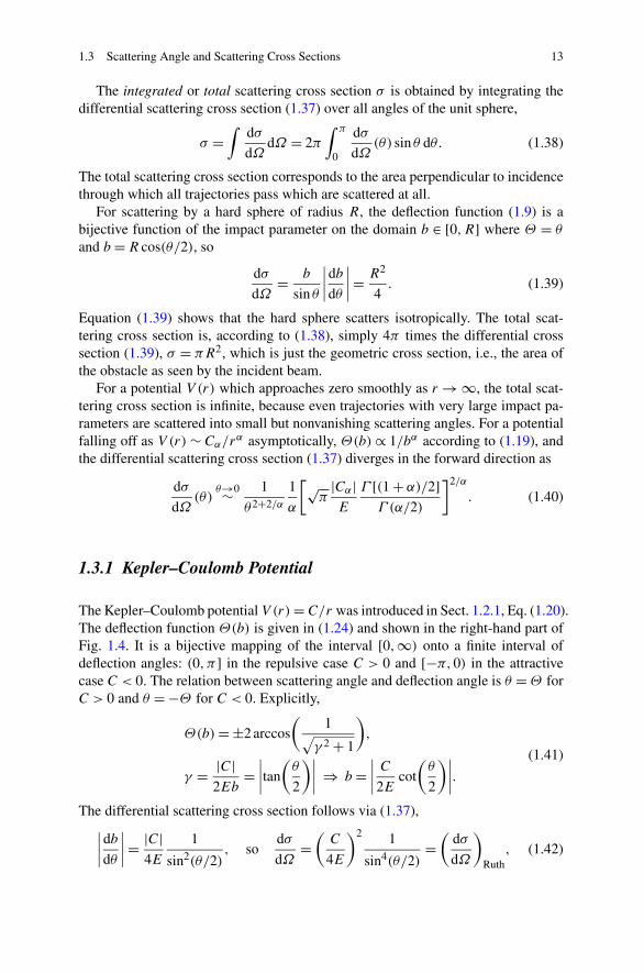
Fig. 1.12 Rutherford crosssection (1.42) for scatteringby the Kepler–Coulombpotential (1.20)

and it is shown in Fig. 1.12. This is the famous Rutherford formula for the dif-ferential cross section in Coulomb scattering. It does not discriminate between therepulsive case C > 0 and the attractive case C < 0.

1.3.2 Inverse-Power Potentials

Inverse-power potentials V (r) = Cα/rα were introduced in Sect. 1.2.2, Eq. (1.25).The deflection function is shown for the example α = 4 in the right-hand part ofFig. 1.6. For the repulsive case, Cα > 0, the deflection function Θ(b) is a bijectivemapping of the interval [0,∞) onto [0,π) and Θ = θ . The scattering cross sectiondiverges in the forward direction according to (1.40) and is a monotonically de-creasing function of the scattering angle. For an attractive inverse-power potentialwith α < 2, there is no centrifugal barrier, and the scattering cross section is also amonotonically decreasing function of θ .

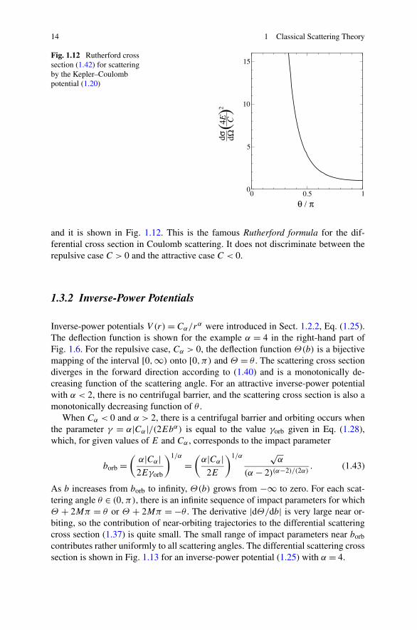
When Cα < 0 and α > 2, there is a centrifugal barrier and orbiting occurs whenthe parameter γ = α|Cα|/(2Ebα) is equal to the value γorb given in Eq. (1.28),which, for given values of E and Cα , corresponds to the impact parameter

borb =(

α|Cα|2Eγorb

)1/α

=(

α|Cα|2E

)1/α √α

(α − 2)(α−2)/(2α). (1.43)

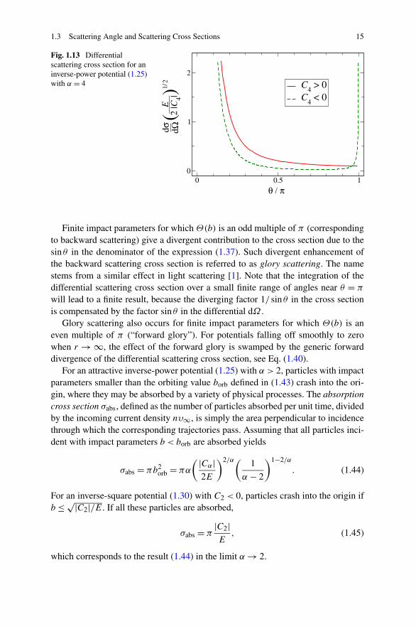
As b increases from borb to infinity, Θ(b) grows from −∞ to zero. For each scat-tering angle θ ∈ (0,π), there is an infinite sequence of impact parameters for whichΘ + 2Mπ = θ or Θ + 2Mπ = −θ . The derivative |dΘ/db| is very large near or-biting, so the contribution of near-orbiting trajectories to the differential scatteringcross section (1.37) is quite small. The small range of impact parameters near borb

contributes rather uniformly to all scattering angles. The differential scattering crosssection is shown in Fig. 1.13 for an inverse-power potential (1.25) with α = 4.


Fig. 1.13 Differentialscattering cross section for aninverse-power potential (1.25)with α = 4

Finite impact parameters for which Θ(b) is an odd multiple of π (correspondingto backward scattering) give a divergent contribution to the cross section due to thesin θ in the denominator of the expression (1.37). Such divergent enhancement ofthe backward scattering cross section is referred to as glory scattering. The namestems from a similar effect in light scattering [1]. Note that the integration of thedifferential scattering cross section over a small finite range of angles near θ = π

will lead to a finite result, because the diverging factor 1/ sin θ in the cross sectionis compensated by the factor sin θ in the differential dΩ .

Glory scattering also occurs for finite impact parameters for which Θ(b) is aneven multiple of π (“forward glory”). For potentials falling off smoothly to zerowhen r → ∞, the effect of the forward glory is swamped by the generic forwarddivergence of the differential scattering cross section, see Eq. (1.40).

For an attractive inverse-power potential (1.25) with α > 2, particles with impactparameters smaller than the orbiting value borb defined in (1.43) crash into the ori-gin, where they may be absorbed by a variety of physical processes. The absorptioncross section σabs, defined as the number of particles absorbed per unit time, dividedby the incoming current density nυ∞, is simply the area perpendicular to incidencethrough which the corresponding trajectories pass. Assuming that all particles inci-dent with impact parameters b < borb are absorbed yields

σabs = πb2orb = πα

( |Cα|2E

)2/α(1

α − 2

)1−2/α

. (1.44)

For an inverse-square potential (1.30) with C2 < 0, particles crash into the origin ifb ≤ √|C2|/E. If all these particles are absorbed,

σabs = π|C2|E

, (1.45)

which corresponds to the result (1.44) in the limit α → 2.


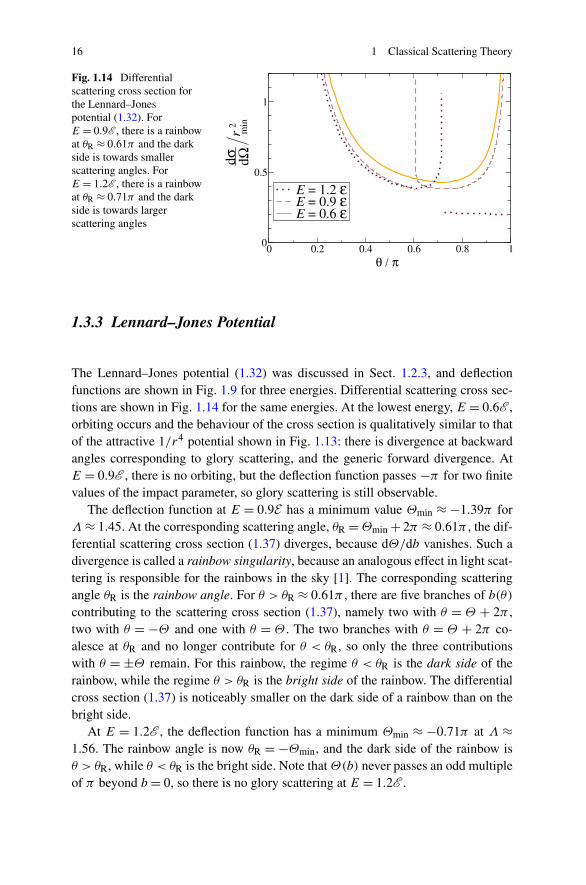
Fig. 1.14 Differentialscattering cross section forthe Lennard–Jonespotential (1.32). ForE = 0.9E , there is a rainbowat θR ≈ 0.61π and the darkside is towards smallerscattering angles. ForE = 1.2E , there is a rainbowat θR ≈ 0.71π and the darkside is towards largerscattering angles

1.3.3 Lennard–Jones Potential

The Lennard–Jones potential (1.32) was discussed in Sect. 1.2.3, and deflectionfunctions are shown in Fig. 1.9 for three energies. Differential scattering cross sec-tions are shown in Fig. 1.14 for the same energies. At the lowest energy, E = 0.6E ,orbiting occurs and the behaviour of the cross section is qualitatively similar to thatof the attractive 1/r4 potential shown in Fig. 1.13: there is divergence at backwardangles corresponding to glory scattering, and the generic forward divergence. AtE = 0.9E , there is no orbiting, but the deflection function passes −π for two finitevalues of the impact parameter, so glory scattering is still observable.

The deflection function at E = 0.9E has a minimum value Θmin ≈ −1.39π forΛ ≈ 1.45. At the corresponding scattering angle, θR = Θmin + 2π ≈ 0.61π , the dif-ferential scattering cross section (1.37) diverges, because dΘ/db vanishes. Such adivergence is called a rainbow singularity, because an analogous effect in light scat-tering is responsible for the rainbows in the sky [1]. The corresponding scatteringangle θR is the rainbow angle. For θ > θR ≈ 0.61π , there are five branches of b(θ)

contributing to the scattering cross section (1.37), namely two with θ = Θ + 2π ,two with θ = −Θ and one with θ = Θ . The two branches with θ = Θ + 2π co-alesce at θR and no longer contribute for θ < θR, so only the three contributionswith θ = ±Θ remain. For this rainbow, the regime θ < θR is the dark side of therainbow, while the regime θ > θR is the bright side of the rainbow. The differentialcross section (1.37) is noticeably smaller on the dark side of a rainbow than on thebright side.

At E = 1.2E , the deflection function has a minimum Θmin ≈ −0.71π at Λ ≈1.56. The rainbow angle is now θR = −Θmin, and the dark side of the rainbow isθ > θR, while θ < θR is the bright side. Note that Θ(b) never passes an odd multipleof π beyond b = 0, so there is no glory scattering at E = 1.2E .

1.4 Classical Scattering in Two Spatial Dimensions 17

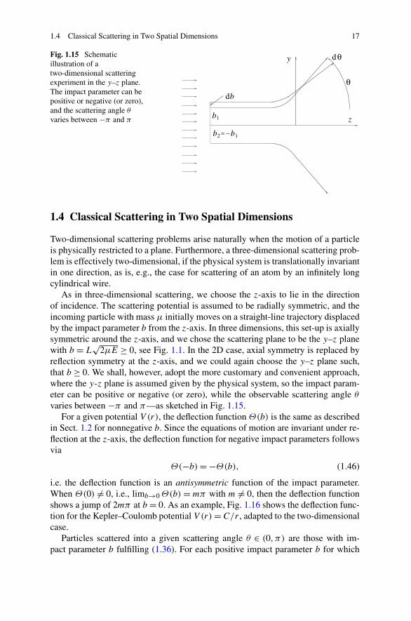
Fig. 1.15 Schematicillustration of atwo-dimensional scatteringexperiment in the y–z plane.The impact parameter can bepositive or negative (or zero),and the scattering angle θ

varies between −π and π

1.4 Classical Scattering in Two Spatial Dimensions

Two-dimensional scattering problems arise naturally when the motion of a particleis physically restricted to a plane. Furthermore, a three-dimensional scattering prob-lem is effectively two-dimensional, if the physical system is translationally invariantin one direction, as is, e.g., the case for scattering of an atom by an infinitely longcylindrical wire.

As in three-dimensional scattering, we choose the z-axis to lie in the directionof incidence. The scattering potential is assumed to be radially symmetric, and theincoming particle with mass μ initially moves on a straight-line trajectory displacedby the impact parameter b from the z-axis. In three dimensions, this set-up is axiallysymmetric around the z-axis, and we chose the scattering plane to be the y–z planewith b = L

√2μE ≥ 0, see Fig. 1.1. In the 2D case, axial symmetry is replaced by

reflection symmetry at the z-axis, and we could again choose the y–z plane such,that b ≥ 0. We shall, however, adopt the more customary and convenient approach,where the y-z plane is assumed given by the physical system, so the impact param-eter can be positive or negative (or zero), while the observable scattering angle θ

varies between −π and π—as sketched in Fig. 1.15.For a given potential V (r), the deflection function Θ(b) is the same as described

in Sect. 1.2 for nonnegative b. Since the equations of motion are invariant under re-flection at the z-axis, the deflection function for negative impact parameters followsvia

Θ(−b) = −Θ(b), (1.46)

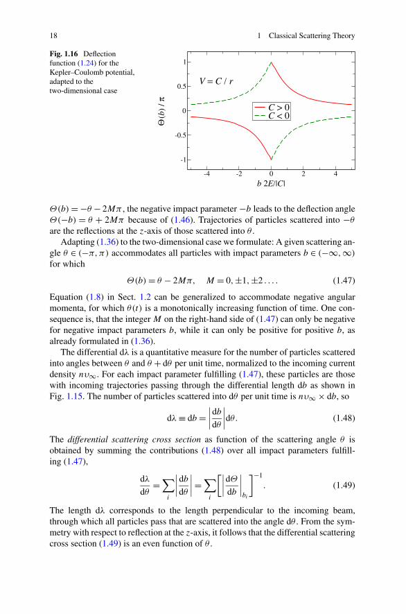
i.e. the deflection function is an antisymmetric function of the impact parameter.When Θ(0) �= 0, i.e., limb→0 Θ(b) = mπ with m �= 0, then the deflection functionshows a jump of 2mπ at b = 0. As an example, Fig. 1.16 shows the deflection func-tion for the Kepler–Coulomb potential V (r) = C/r , adapted to the two-dimensionalcase.

Particles scattered into a given scattering angle θ ∈ (0,π) are those with im-pact parameter b fulfilling (1.36). For each positive impact parameter b for which


Fig. 1.16 Deflectionfunction (1.24) for theKepler–Coulomb potential,adapted to thetwo-dimensional case

Θ(b) = −θ − 2Mπ , the negative impact parameter −b leads to the deflection angleΘ(−b) = θ + 2Mπ because of (1.46). Trajectories of particles scattered into −θ

are the reflections at the z-axis of those scattered into θ .Adapting (1.36) to the two-dimensional case we formulate: A given scattering an-

gle θ ∈ (−π,π) accommodates all particles with impact parameters b ∈ (−∞,∞)

for which

Θ(b) = θ − 2Mπ, M = 0,±1,±2 . . . . (1.47)

Equation (1.8) in Sect. 1.2 can be generalized to accommodate negative angularmomenta, for which θ(t) is a monotonically increasing function of time. One con-sequence is, that the integer M on the right-hand side of (1.47) can only be negativefor negative impact parameters b, while it can only be positive for positive b, asalready formulated in (1.36).

The differential dλ is a quantitative measure for the number of particles scatteredinto angles between θ and θ + dθ per unit time, normalized to the incoming currentdensity nυ∞. For each impact parameter fulfilling (1.47), these particles are thosewith incoming trajectories passing through the differential length db as shown inFig. 1.15. The number of particles scattered into dθ per unit time is nυ∞ × db, so

dλ ≡ db =∣∣∣∣db

dθ

∣∣∣∣dθ. (1.48)

The differential scattering cross section as function of the scattering angle θ isobtained by summing the contributions (1.48) over all impact parameters fulfill-ing (1.47),

dλ

dθ=

∑

i

∣∣∣∣db

dθ

∣∣∣∣ =∑

i

[∣∣∣∣dΘ

db

∣∣∣∣bi

]−1

. (1.49)

The length dλ corresponds to the length perpendicular to the incoming beam,through which all particles pass that are scattered into the angle dθ . From the sym-metry with respect to reflection at the z-axis, it follows that the differential scatteringcross section (1.49) is an even function of θ .

1.4 Classical Scattering in Two Spatial Dimensions 19

The integrated or total scattering cross section is obtained by integrating thedifferential cross section (1.49) over all scattering angles:

λ =∫ π

−π

dλ

dθdθ. (1.50)

It corresponds to the length perpendicular to the incoming beam, through which allparticles pass that are scattered at all.

The formulae (1.49) and (1.50) for scattering cross sections in 2D differ from thecorresponding formulae (1.37) and (1.38) in 3D in that they are missing the factorbi/ sin θ coming from the definition of the solid angle. So, although the deflectionfunction in 2D scattering is the same as in 3D—supplemented by Eq. (1.46) to ac-commodate negative impact parameters—the scattering cross sections for analogoussystems in 2D and 3D do show differences.

Scattering by a hard sphere of radius R in 3D corresponds in 2D to the scatteringby a hard disc of radius R, and Fig. 1.2 in Sect. 1.2 can be used as illustration in thiscase as well. The deflection function is given by (1.9) with (1.46), so b = R cos(θ/2)

and the differential cross section is, according to (1.49),

dλ

dθ=

∣∣∣∣db

dθ

∣∣∣∣ = R

2

∣∣∣∣sin

(θ

2

)∣∣∣∣. (1.51)

Note that scattering by a hard disc is, in contrast to scattering by a sphere, notisotropic. It is peaked at backward angles, θ → ±π , and it vanishes towards forwardangles θ → 0. The depletion at forward angles is easily understood considering thatparticles scattered into small angles hit the disc near the edge of its projection ontothe line perpendicular to incidence, i.e. for b near ±R. In 3D, a whole circle of im-pact parameters with b near R and azimuthal angles from zero to 2π contributes toscattering into small angles. The integrated cross section for scattering by the harddisc is

λ = R

2

∫ π

−π

∣∣∣∣sin

(θ

2

)∣∣∣∣dθ = 2R, (1.52)

which is the geometric cross section, i.e., the length occupied by the disc in the pathof the incident particles.

As in 3D scattering, the integrated cross section is infinite for a potential falling

off smoothly as r → ∞. For V (r)r→∞∼ Cα/rα , the deflection function behaves

according to (1.19) and the differential scattering cross section (1.49) diverges inthe forward direction as

dλ

dθ

θ→0∼ 1

|θ |1+1/α

1

α

[√π

|Cα|E

Γ [(1 + α)/2]Γ (α/2)

]1/α

. (1.53)

Comparing the forward divergence in 2D (1.53) and 3D (1.40) gives the appealinglysimple result,

[dλ

dθ(θ)

]

2D

θ→0∼√

1

α

[dσ

dΩ

(|θ |)]

3D. (1.54)


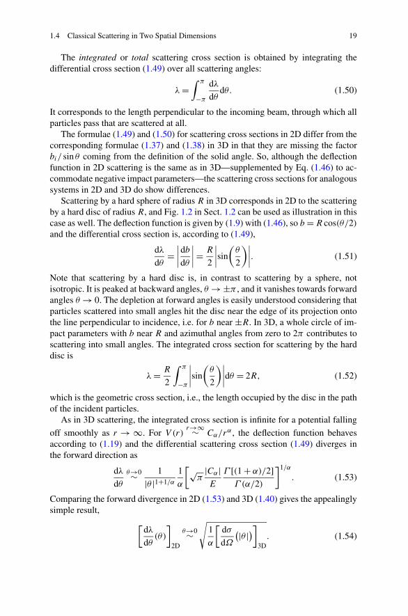
Fig. 1.17 Differentialscattering cross section in twodimensions for aninverse-power potential (1.25)with α = 4

For the Kepler–Coulomb potential V (r) = C/r , the deflection function is givenanalytically in (1.24) and displayed for the 2D situation in Fig. 1.16. The differentialscattering cross section in 2D follows immediately via (1.49),

dλ

dθ= |C|

4E

1

sin2(θ/2). (1.55)

In this case, the relation (1.54), with α = 1, is not only valid asymptotically forθ → 0; it is an equality for all scattering angles.

The cross sections for the other examples discussed in Sect. 1.3 can also be de-rived via (1.49) using the deflection functions given in Sect. 1.2. Apart from theslower divergence at forward angles, a main difference is the absence of the glorysingularity, which is due to the factor 1/ sin θ in the 3D case. A main manifesta-tion of orbiting and near-orbiting situations in 3D scattering, namely glory scat-tering at backward angles, is thus missing in the 2D cross sections. Figure 1.17shows the differential scattering cross section (1.49) for an inverse-power potentialV (r) = C4/r4. The ordinate is labelled with the cross section in units of the length(2|C4|/E)1/4.

For scattering by an attractive inverse-power potential V (r) = Cα/rα , withα > 2, orbiting occurs for impact parameters |b| = borb, with borb given by (1.43).Assuming that all particles with impact parameters |b| < borb are absorbed, the ab-sorbtion cross section is

λabs = 2borb. (1.56)

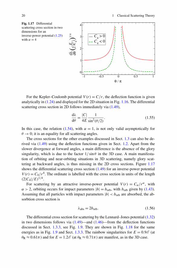
The differential cross section for scattering by the Lennard–Jones potential (1.32)in two dimensions follows via (1.49)—and (1.46)—from the deflection functionsdiscussed in Sect. 1.3.3, see Fig. 1.9. They are shown in Fig. 1.18 for the sameenergies as in Fig. 1.9 and Sect. 1.3.3. The rainbow singularities for E = 0.9E (atθR ≈ 0.61π ) and for E = 1.2E (at θR ≈ 0.71π ) are manifest, as in the 3D case.

References 21

Fig. 1.18 Differentialscattering cross section in twodimensions for theLennard–Jonespotential (1.32). ForE = 0.9E , there are rainbowsat |θ | = θR ≈ 0.61π and thedark sides are towards smallervalues of |θ |. For E = 1.2E ,there are rainbows at|θ | = θR ≈ 0.71π and thedark sides are towards largervalues of |θ |

References

1. Adam, J.A.: The mathematical physics of rainbows and glories. Phys. Rep. 356, 229–365(2002)

2. Landau, L.D., Lifshitz, E.M.: Course of Theoretical Physics. Mechanics, vol. 1. 3rd edn.Butterworth-Heinemann, Stoneham (1976)

Documents

Chapter 1 Classical Scattering Theory - College of Charlestonwilliamsgj.people.cofc.edu/Scattering Theory.pdfChapter 1 Classical Scattering Theory 1.1 Relative Motion of Projectile