Chapter 1 Computational Methods for the Fourier Analysis ... · Chapter 1 Computational Methods for the Fourier Analysis of Sparse High-Dimensional Functions Lutz K ammerer, Stefan

Chapter 1

Computational Methods for theFourier Analysis of SparseHigh-Dimensional Functions

Lutz Kammerer, Stefan Kunis, Ines Melzer, Daniel Potts, and Toni Volkmer

Abstract A straightforward discretisation of high-dimensional problems of-ten leads to a curse of dimensions and thus the use of sparsity has become apopular tool. Efficient algorithms like the fast Fourier transform (FFT) haveto be customised to these thinner discretisations and we focus on two ma-jor topics regarding the Fourier analysis of high-dimensional functions: Wepresent stable and effective algorithms for the fast evaluation and reconstruc-tion of trigonometric polynomials with frequencies supported on an index setI ⊂ Zd.

1.1 Introduction

Let d ∈ N be the spatial dimension and Td = Rd/Zd ' [0, 1)d denote thetorus. We consider trigonometric polynomials f : Td → C with Fourier co-efficients fk ∈ C supported on the frequency index set I ⊂ Zd of finitecardinality. The evaluation of the trigonometric polynomial

f(x) =∑k∈I

fk e2πik·x (1.1)

at a sampling set X ⊂ Td of finite cardinality can be written as the matrix-vector product

Stefan Kunis∗, Ines MelzerInstitut fur Mathematik, Universitat Osnabruck, ∗and Institute of Computational Biology,

Helmholtz Zentrum Munchen, Germanye-mail: stefan.kunis,[email protected]

Lutz Kammerer and Daniel Potts and Toni VolkmerFakultat fur Mathematik, Technische Universitat Chemnitz, Germany

e-mail: lutz.kaemmerer,daniel.potts,[email protected]

1

2 Lutz Kammerer, Stefan Kunis, Ines Melzer, Daniel Potts, and Toni Volkmer

f = A f , f = (f(x))x∈X ∈ C|X |, f = (fk)k∈I ∈ C|I|, (1.2)

with the Fourier matrix A = A(I,X ) =(

e2πik·x)x∈X ,k∈I ∈ C|X |×|I|.

We are interested in the following two problems:

1. Evaluation: given a support I ⊂ Zd, Fourier coefficients fk ∈ C, k ∈ I,and sampling nodes X = x` ∈ Td : ` = 0, . . . , L − 1, evaluate thetrigonometric polynomial (1.1) efficiently, i.e., compute f = Af by meansof a fast algorithm,

2. Reconstruction: given a support of Fourier coefficients I ⊂ Zd, construct aset of sampling nodes X ⊂ Td with small cardinality L = |X | which allowsfor the unique and stable reconstruction of all trigonometric polynomials(1.1) from their sampling values f(x`). In particular, solve the system oflinear equations Af ≈ f .

As an extension to the reconstruction problem, the efficient approximatereconstruction of a smooth function from subspaces of the Wiener algebra bya trigonometric polynomial (1.1), which guarantees a good approximation tothe function, was considered in [37].

1.2 Evaluation of trigonometric polynomials

Clearly, the straightforward evaluation of the trigonometric polynomial (1.1)in all sampling nodes X ⊂ Td, or equivalently the matrix vector multiplication(1.2), takes O(|X | · |I|) floating point operations. For special index sets fasteralgorithms have been constructed as detailed subsequently.

1.2.1 FFT and nonequispaced FFT

We consider trigonometric polynomials supported on the full grid, i.e., withFourier coefficients fk are defined on the full d-dimensional set I := Gdn =

Zd ∩×dj=1(−2n−1, 2n−1] of refinement n ∈ N and bandwidth N = 2n with

the cardinality |I| = Nd. The evaluation of the trigonometric polynomial

f(x) =∑k∈Gdn

fk e2πik·x (1.3)

at all sampling nodes of an equispaced grid x ∈ X = (2−nGdn mod 1), with thecardinality |X | = Nd, requires only O(2ndn) = O(Nd logN) by the famousfast Fourier transform (FFT). A well understood generalisation considers anarbitrary sampling set X = x` ∈ Td : ` = 0, . . . , L− 1 and leads to the so-

1 Sparse Fast Fourier Transforms 3

called nonequispaced FFT which takes O(2ndn+ | log ε|dL) = O(Nd logN +| log ε|dL) floating point operations for a target accuracy ε > 0, see e.g. [16,5, 59, 51, 39] and the references therein. In both cases, already the huge

cardinality of the support Gdn of the Fourier coefficients fk causes immensecomputational costs for high dimensions d even for moderate refinement n.Hence, we restrict the index set I to smaller sets.

1.2.2 Hyperbolic cross FFT

Functions of dominating mixed smoothness can be well approximated bytrigonometric polynomials supported on reduced frequency index sets, socalled dyadic hyperbolic crosses

I = Hdn :=

⋃j∈Nd0‖j‖1=n

(Zd ∩

d×l=1

(−2jl−1, 2jl−1]

)

of dimension d and refinement n, cf. [57]. Compared to the trigonometricpolynomial in (1.3), we strongly reduce the number of used Fourier coefficients|Hd

n| = O(2nnd−1) 2nd. A natural spatial discretisation of trigonometricpolynomials supported on the dyadic hyperbolic cross Hd

n is given by thesparse grid

X = Sdn :=⋃j∈Nd0‖j‖1=n

d×l=1

2−jl(N0 ∩ [0, 2jl)).

The cardinalities of the sparse grid and the dyadic hyperbolic cross are |Sdn| =|Hd

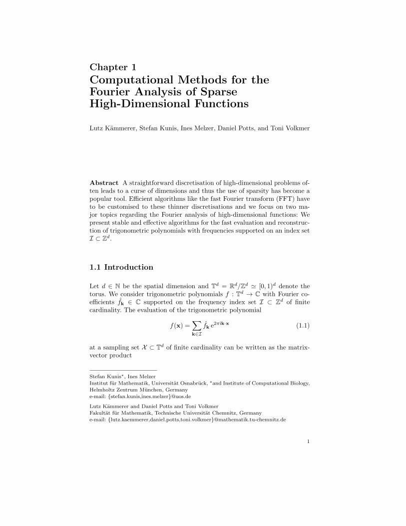
n| = O(2nnd−1). Fig. 1.1a(left) shows an example for a two-dimensionaldyadic hyperbolic cross and Fig. 1.1a(right) depicts the corresponding sparsegrid of identical cardinality. Based on [3, 27] there exists a fast algorithmfor evaluating the trigonometric polynomial with frequencies supported onthe hyperbolic cross Hd

n at all x ∈ Sdn in O(2nnd) floating point operations,called hyperbolic cross fast Fourier transform (HCFFT). A generalisation tosparser index set, i.e., to index sets for so called energy-norm based hyperboliccrosses, is presented in [22].

1.2.3 Lattice and generated set FFT

Using lattices as sampling set X is motivated from the numerical integrationof functions of many variables by lattice rules, see [58, 47, 14] for an introduc-tion. In contrast to general lattices which may be spanned by several vectors,


−15 0 16−15

0

16

0 0.5 10

0.5

1

H25 S2

5

0 0.5 10

0.5

1

0 0.5 10

0.5

1

r = M−1(1, 17)> r = (0.7907, 0.9128)>

Fig. 1.1a Dyadic hyperbolic cross H25

(left) and sparse grid S25 (right).

Fig. 1.1b Rank-1 lattice (left) and gen-erated set Λ(r,M) (right), M = 163.

we only consider so-called rank-1 lattices and a generalisation of this conceptcalled generated sets [32]. For a given number L ∈ N of sampling nodes anda generating vector r ∈ Rd, we define the generated set

X = Λ(r, L) := x` = `r mod 1, ` = 0, . . . , L− 1 ⊂ Td.

For ` = 0, . . . , L − 1, the evaluation of a d-variate trigonometric polynomialsupported on an arbitrary frequency index set I simplifies dramatically since

f(x`) =∑k∈I

fk e2πik·x` =∑k∈I

fk e2πi`k·r =∑y∈Y

gy e2πi`y, (1.4)

with some set Y = k · r mod 1 : k ∈ I ⊂ T and the aliased coefficients

gy =∑

k·r≡y (mod 1)

fk. (1.5)

Using a one-dimensional adjoint nonequispaced FFT [39], this takesO(L logL + (d + | log ε|)|I|) floating point operations for a target accuracyε > 0. Moreover, given L ∈ N and a generating vector r = z/L, z ∈ Zd,the sampling scheme Λ(r, L) is called rank-1 lattice and the computationalcosts of the evaluation reduce to O(L logL+ d|I|) by applying a one dimen-sional FFT. We stress on the fact that in both cases, the computational costsonly depend on the number L of samples subsequent to the aliasing step (1.5)which takes d|I| floating point operations. Fig. 1.1b(left) and Fig. 1.1b(right)show an example for a two-dimensional rank-1 lattice and generated set, re-spectively.

1.2.4 Butterfly sparse FFT

Another generalisation of the classical FFT to nonequispaced nodes has beensuggested in [1, 62, 40]. While the above mentioned nonequispaced FFT stillrelies on a equispaced FFT, the so-called butterfly scheme only relies on


local low rank approximations of the complex exponentials - in particularthis locality allows for its application to sparse data. The idea of local lowrank approximations can be traced back at least to [21, 63, 4, 26] for smoothkernel functions and to [45, 64, 48, 61, 13] for oscillatory kernels. In a linearalgebra setting, it was pointed out in [17] that certain blocks of the Fouriermatrix are approximately of low rank.

We consider real frequencies I ⊂ [0, 2n)d and nonequispaced evaluationnodes x` ∈ X ⊂ [0, 1)d in

f(x`) =∑k∈I

fk e2πik·x` , ` = 0, . . . , L− 1. (1.6)

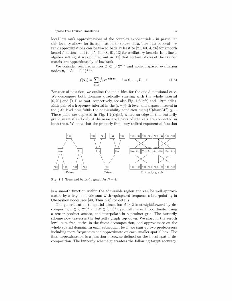
For ease of notation, we outline the main idea for the one-dimensional case.We decompose both domains dyadically starting with the whole interval[0, 2n) and [0, 1) as root, respectively, see also Fig. 1.2(left) and 1.2(middle).Each pair of a frequency interval in the (n−j)-th level and a space interval inthe j-th level now fulfils the admissibility condition diam(I ′)diam(X ′) ≤ 1.These pairs are depicted in Fig. 1.2(right), where an edge in this butterflygraph is set if and only if the associated pairs of intervals are connected inboth trees. We note that the properly frequency shifted exponential function

X00

X10 X11

X20 X21 X22 X23 I00

I10 I11

I20 I21 I22 I23 X00,I20 X00,I21 X00,I22 X00,I23

X10,I10 X10,I11 X11,I10 X11,I11

X20,I00 X21,I00 X22,I00 X23,I00

X -tree. I-tree. Butterfly graph.

Fig. 1.2 Trees and butterfly graph for N = 4.

is a smooth function within the admissible region and can be well approxi-mated by a trigonometric sum with equispaced frequencies interpolating inChebyshev nodes, see [40, Thm. 2.6] for details.

The generalisation to spatial dimension d ≥ 2 is straightforward by de-composing I ⊂ [0, 2n)d and X ⊂ [0, 1)d dyadically in each coordinate, usinga tensor product ansatz, and interpolate in a product grid. The butterflyscheme now traverses the butterfly graph top down. We start in the zerothlevel, sum frequencies in the finest decomposition, and approximate on thewhole spatial domain. In each subsequent level, we sum up two predecessorsincluding more frequencies and approximate on each smaller spatial box. Thefinal approximation is a function piecewise defined on the finest spatial de-composition. The butterfly scheme guarantees the following target accuracy.


Theorem 1.1. ([40, Thm. 3.1]). Let d, n, p ∈ N, p ≥ 5, I ⊂ [0, 2n)d,X ⊂ [0, 1)d, and the trigonometric sum f as in (1.6), then the butterflyapproximation g obeys the error estimate

‖f − g‖∞ ≤(Cp + 1)(C

d(n+1)p − 1)

Cp − 1cp‖f‖1.

The constants are explicitly given by

Kp :=

(2π2

(1−cos 2πp−1 )(p−1)2

)p−1, Kp ≤

π4

16, lim

p→∞Kp = 1,

Cp :=√Kp

(1 + 2

π log p), cp :=

1

πp

(π

p− 1

)p.

In particular, the butterfly scheme achieves relative error at most ε if thelocal expansion degree fulfils p ≥ max10, 2| log ε|, 2d(n+ 1).

In case 1 ≤ t < d and |X | = |I| = 2nt well distributed sets on smootht-dimensional manifolds, the dyadic decompositions of the sets remain sparse.Consequently, the butterfly graph, which represents the admissible pairswhere computations are performed, remains sparse as well and the computa-tion of (1.6) takes O(2ntn(n+ | log ε|)d+1) floating point operations only.

1.3 Reconstruction of trigonometric polynomials

Beyond the fast evaluation of Fourier expansions, the sampling problem isconcerned with the recovery of the Fourier coefficients fk ∈ C from a sequenceof function samples. This inverse transform constructs a trigonometric poly-nomial (1.1) such that for given data points (x`, f`) ∈ Td×C, ` = 0, . . . , L−1,the approximate identity

f (x`) ≈ f`is fulfilled. Thus, we aim to solve the linear system of equations Af ≈ f forthe vector of Fourier coefficients f ∈ C|I|. In contrast to the ordinary Fouriermatrix, its generalized analogue A is in general neither unitary nor square.The meaningful variants of this reconstruction problem include

1. the weighted least squares approximation

‖f −Af‖2W =

L−1∑`=0

w`|f` − f(x`)|2f→ min, (1.7)

for the over-determined case |I| < |X |, where the weights w` compensatefor clusters in the sampling set,

2. the optimal interpolation problem


‖f‖2W−1 =

∑k∈I

|fk|2

wk

f→ min subject to Af = f , (1.8)

for the under-determined case |I| > |X |, where the weights wk damp high-frequency components, and

3. the sparse recovery problem

‖f‖0 = |k ∈ I : fk 6= 0| f→ min subject to Af = f , (1.9)

for the under-determined case |I| > |X |.

The main tool in iterative methods to solve these three problems is the useof fast matrix-vector multiplications with A and A∗ and bounding involvedcondition numbers uniformly.

1.3.1 FFT and nonequispaced FFT

The reconstruction of the Fourier coefficients fk, k ∈ Gdn from samplingvalues of an equispaced grid x ∈ X = (2−nGdn mod 1), see (1.3), can berealized by the inverse fast Fourier transform, since the Fourier matrix F :=A(2−nGdn, G

dn) has orthogonal columns, and takes O(Nd logN) floating point

operations. This is no longer true for the nonequispaced Fourier matrix givenby

A := A(X , Gdn) =(

e2πik·x`)`=0,...,L−1,k∈Gdn

.

Here, we use an iterative algorithm since the fast matrix times vector multi-plication with the matrix A and A> takes only O(2ndn+ | log ε|dL) floatingpoint operations, see [39]. The conditioning of the reconstruction problemsrelies on the uniformity of X , measured by the mesh norm and the separationdistance

δ := 2 maxx∈Td

minj=0,...,L−1

dist(xj ,x), q := minj,l=0,...,L−1;j 6=l

dist (xj ,xl) ,

where dist (x,x0) := minj∈Zd ‖(x + j)− x0‖∞, respectively.For the overdetermined case Nd < L, it has been proven in [24] that the

reconstruction problem (1.7) has a unique solution if N < ( πlog 2 d δ)

−1. Thesolution is computed iteratively by means of the conjugate gradient methodin [18, 2, 23], where the multilevel Toeplitz structure of A>WA is usedfor fast matrix vector multiplications. Slightly more stable with respect torounding errors is the CGNR method, cf. [6, pp. 288], which iterates theoriginal residual rl = y −Afl instead of the residual A>Wrl of the normalequations. Further analysis of the numerical stability of the least squaresapproximation (1.7) relies on so-called Marcinkiewicz-Zygmund inequalities


which establish norm equivalences between a trigonometric polynomial andits samples, see e.g. [60, 44, 19, 38] and references therein for specific variants.

For the underdetermined case Nd > L, the optimal interpolation problem(1.8) has been shown to be stable in [41] if the sampling set is well separatedwith respect to the polynomial degree and the weights wk are constructedby means of a so-called smoothness-decay principle. In particular, we provedthat the nonequispaced Fourier matrix A has full rank L for every polynomialdegree N > 2 d q−1 and proposed to solve problem (1.8) by a version of theconjugate gradient method in combination with the nonequispaced FFT toefficiently perform each iteration step.

1.3.2 Hyperbolic cross FFT

The inverse HCFFT is not an orthogonal transform, but a fast algorithmis developed by reverting all steps of the HCFFT, see [3, 27], which makesthis spatial discretisation most attractive in terms of efficiency. The inverseHCFFT requires also only O(2nnd) floating point operations. However, weproved in [35] that this transform is mildly ill conditioned, i.e.,

cd2n2 n

2d−32 ≤ cond2A(Hd

n, Sdn) ≤ Cd2

n2 n2d−2, n→∞,

cnd2n ≤ cond2A(Hd

n, Sdn) ≤ Cnd2n, d→∞.

In particular, we loose more than 5 decimal digits of accuracy already ford = 10 and n = 5 in the worst case.

1.3.3 Lattice and generated set FFT

As pointed out in Section 1.2.3, the evaluation of trigonometric polynomialswith frequencies supported on an arbitrary index set I, i.e., the mappingfrom the index set I in frequency domain to the rank-1 lattice in spatialdomain reduces to a single one-dimensional FFT and thus can be computedvery efficiently and stable. For the inverse transform, mapping the samplesof a trigonometric polynomial to its Fourier coefficients on a specific fre-quency index set, we discuss the recently presented necessary and sufficientconditions on rank-1 lattices allowing a stable reconstruction of trigonomet-ric polynomials supported on hyperbolic crosses and the generalisation toarbitrary index sets in the frequency domain. We suggest approaches for de-termining suitable rank-1 lattices using a component-by-component strategy[33, 12]. In conjunction with numerical found lattices, we show that this newmethod outperforms the classical hyperbolic cross FFT for realistic problemsizes [36].


The use of generated sets, a generalisation of rank-1 lattices, as spatialdiscretisations offers an additional suitable possibility for sampling sparsetrigonometric polynomials. The fast computation of trigonometric polynomi-als on generated sets can be realized using the nonequispaced fast Fouriertransform (NFFT), cf. [39]. A simple sufficient condition on a generated setΛ(r, L) allows the fast, unique and stable reconstruction of the frequenciesof a d-dimensional trigonometric polynomial from its samples along Λ(r, L).In contrast to searching for suitable rank-1 lattices, we can use continuousoptimization methods in order to determine generated sets that are suitablefor reconstruction, see [32].

Reconstruction using rank-1 lattices. In order to state constructiveexistence results for reconstructing rank-1 lattices, i.e., rank-1 lattices whichallow the unique reconstruction of trigonometric polynomials supported on afixed frequency index set I, we define the difference set

D(I) := k− l : k, l ∈ I

of the frequency index set I. As a consequence of [34, Cor. 1] we formulatethe following

Theorem 1.2. Let I ⊂ k ∈ Zd : k−a ∈ [0, |I|−1]d for a fixed a ∈ Zd beinga frequency index set of finite cardinality. Then there exists a reconstructingrank-1 lattice of prime cardinality L,

|I| ≤ L ≤ |D(I)| ≤ |I|2, (1.10)

such that all trigonometric polynomials f with frequencies supported on I canbe reconstructed from the sampling values (f(x))x∈Λ(r,L). Moreover, the corre-

sponding generating vector r ∈ L−1Zd can be determined using a component–by–component strategy and the reconstruction of the Fourier coefficients canbe realized by a single one-dimensional FFT of length L, and thus takesO(L logL+ d|I|) floating point operations.

Proof. The result follows from [34, Cor. 1], Bertrand’s postulate, and equa-tions (1.4) and (1.5). ut

We stress on the fact, that [34, Cor. 1] is a more general result on arbitraryfrequency index sets I. Some simple additional assumptions on L allow toreplace the condition I ⊂ k ∈ Zd : k−a ∈ [0, |I|−1]d by I ⊂ Zd, |I| <∞.

In fact, the cardinality of the difference set D(I) is the theoretical upperbound in (1.10) for the number of samples needed to reconstruct trigonomet-ric polynomials with frequencies supported on the index set I using a rank-1lattice. This cardinality depends mainly on the structure of I.

Example 1.1. Let I = Idp,N := k ∈ Zd : ‖k‖p ≤ N, N ∈ N, be the `p-ball,

0 < p ≤ ∞, of size N , see Fig. 1.3. The cardinality of Idp,N is bounded by

cp,dNd ≤ |Idp,N | ≤ CdN

d and cp,dNd ≤ D(Idp,N ) ≤ Cd2

dNd, cp,d, Cd ∈ R,


−16 0 16−16

0

16

I21/2,16

−16 0 16−16

0

16

I21,16

−16 0 16−16

0

16

I22,16

−16 0 16−16

0

16

I2∞,16

Fig. 1.3 Two-dimensional frequency index sets I2p,16 for p ∈ 12, 1, 2,∞.

0 < cp,d ≤ Cd. Consequently, we can find a reconstructing rank-1 lattice of

size L ≤ Cp,d|Idp,N |, Cp,d > 0, using a component-by-component strategy.On the other hand, we obtain for the limit p → 0 the frequency index

set I := k ∈ Zd : ‖k‖1 = ‖k‖∞ ≤ N, N ∈ N, which is supported on thecoordinate axis. We have |I| = 2dN+1 and (2N+1)2 ≤ |D(I)| ≤ (2dN+1)2.Hence, we estimate cd|I|2 ≤ |D(I)|, cd ∈ R, 0 < cd, and the theoretical upperbound on L is quadratic in |I| for fixed dimension d. In fact, reconstructingrank-1 lattices for these specific frequency index sets need at least a numberof L ∈ Ω(N2) nodes, cf. [36, Thm. 3.5]. ut

Example 1.2. More useful frequency index sets in higher dimensions d > 2 areso-called (energy-norm based) hyperbolic crosses, cf. [3, 7, 8]. In particular,we consider frequency index sets I of the form

Id,TN :=

k ∈ Zd : max(1, ‖k‖1)

TT−1

d∏s=1

max(1, |ks|)1

1−T ≤ N

,

with parameter T ∈ [0, 1) and N ∈ N, see Fig. 1.4 for illustration. The fre-

quency index set Id,0N , i.e., T = 0, is in fact a symmetric hyperbolic cross

and frequency index sets Id,TN , T ∈ (0, 1), are called energy-norm based hy-

perbolic crosses. The cardinality of Id,TN can be estimated, cf. [37, Lem. 2.6],by

cd,0N logd−1N ≤ |Id,TN | ≤ Cd,0N logd−1N, for T = 0,

cd,TN ≤ |Id,TN | ≤ Cd,TN, for T ∈ (0, 1),

where cd,T , Cd,T ∈ R, 0 < cd,T ≤ Cd,T . Since the axis cross is a subset of the

considered frequency index sets, i.e., k ∈ Zd : ‖k‖1 = ‖k‖∞ ≤ N ⊂ Id,TN ,

T ∈ [0, 1), we obtain (2N + 1)2 ≤ |D(Id,TN )|. On the other hand, we obtain

upper bounds of the cardinality of the difference set D(Id,TN )

|D(Id,TN )| ≤ Cd,0N2 logd−2N, for T = 0, cf. [33, Thm. 4.8],

|D(Id,TN )| ≤ |Id,TN |2 ≤ C2

d,TN2, for T ∈ (0, 1).


−32 0 32−32

0

32

I2,032

−32 0 32−32

0

32

I2,1/432

−32 0 32−32

0

32

I2,1/232

Fig. 1.4 Two-dimensional frequency index sets I2,T32 for T ∈ 0, 1

4, 12.

Consequently, Theorem 1.2 offers a constructive strategy in order to findreconstructing rank-1 lattices for Id,TN of cardinality L ≤ |D(Id,TN )|. We wouldlike to stress that, at least for T ∈ (0, 1), we are able to construct rank-1lattices of optimal order in N , cf. [33, Lem. 2.1, 2.3, and Cor. 2.4].

For instance, Fig. 1.1b(left) shows a reconstructing rank-1 lattice for thesymmetric hyperbolic cross I2,08 and Fig. 1.1b(right) shows an example for agenerated set, which allows the exact reconstruction of trigonometric poly-nomials with frequencies supported on I2,08 . The condition number of theFourier matrix A(I,X ) is always one when X is a reconstructing rank-1 lat-tice for I, since the columns of the Fourier matrix A(I,X ) are orthogonal.When the frequency index set I = I2,08 and X is the specific generated set inFig. 1.1b(right), then the condition number of the Fourier matrix A(I,X ) isapproximately 2.19. ut

Reconstruction using generated sets. Up to now, we discussed recon-structing rank-1 lattices. We generalized this concept to so-called generatedsets, cf. Section 1.2.3 and determined sufficient and necessary conditions ongenerated sets Λ(r, L) guaranteeing a full rank and stable Fourier matrixA(I, Λ(r, L)) in [32]. In general, the set Y = k · r mod 1 : k ∈ I ⊂ T is ofour main interest, where r ∈ Rd is the generating vector of the generated setΛ(r, L). We determined the necessary condition |Y| = |I| in order to obtaina Fourier matrix A(I, Λ(r, L)) of full column rank.

Theorem 1.3. Let I ⊂ Zd be an arbitrary d-dimensional index set of finitecardinality |I|. Then, the exact reconstruction of a trigonometric polynomialwith frequencies supported on I is possible from only |I| samples using asuitable generated set.

Proof. Let r ∈ Rd be a vector such that

k · r mod 1 6= k′ · r mod 1 for all k,k′ ∈ I, k 6= k′. (1.11)

For instance, Theorem 1.2 guarantees the existence of a reconstructing rank-1 lattice Λ(r, L) for the index set I, where r ∈ L−1Zd fulfills property(1.11). The corresponding Fourier matrix A := (e2πik·x`)`=0,...,L−1; k∈I =


(e(2πik·r)`

)`=0,...,L−1; k∈I is a transposed Vandermonde matrix of (full col-umn) rank |I|. If we use only the first |I| rows of the matrix A and

denote this matrix by A, the matrix A := (e(2πik·r)`

)`=0,...,|I|−1; k∈I =

(e(2πiyj)`

)`=0,...,|I|−1; j=0,...,|I|−1 is a transposed Vandermonde matrix of size|I| × |I|, where yj := kj · r mod 1 and I = k0, . . . ,k|I|−1 in the specifiedorder. Furthermore, the determinant of the transposed Vandermonde matrixA, cf. [31, Sec. 6.1], is det A =

∏1≤k<j≤|I|−1(e2πiyj − e2πiyk) 6= 0 , since

we have e2πik·r 6= e2πik′·r for all k,k′ ∈ I, k 6= k′, due to property (1.11).

This means the transposed Vandermonde matrix A has full rank |I| and isinvertible. ut

Theorem 1.3 states that L = |I| many samples are sufficient to exactlyreconstruct a trigonometric polynomial with frequencies supported on theindex set I. In general, we obtain a large condition number for the Fourier

matrix A := (e(2πik·r)`

)`=0,...,|I|−1; k∈I . Using L > |I| samples, we also ob-tain matrices A(I, Λ(r, L)) of full column rank, since the first |I| rows of thematrix A(I, Λ(r, L)) are linear independent. In practice, growing oversam-pling, i.e., increasing L > |I|, decreases at least an estimator of the conditionnumber of A(I, Λ(r, L)), as published in [32]. In this context, for each gen-erating vector r ∈ Rd bringing |Y| = |I| and constant C > 1 we determineda generated set of size LC such that the Fourier matrix A(I, Λ(r, LC)) hasa condition number of at most C, cf. [32, Cor. 1]. We discuss a nonlinearoptimization strategy in [32] in order to determine generated sets Λ(r, L)of relatively small cardinality bringing a Fourier matrix A(I, Λ(r, L)) withsmall condition number.

The reconstruction of trigonometric polynomials with frequencies sup-ported on an fixed index set I from samples along a generated set can be re-alized solving the normal equation, which can be done in a fast way using theone-dimensional NFFT and a conjugate gradient (CG) method. One step ofthe CG method needs one NFFT of length L and one adjoint NFFT of lengthL. Consequently, one CG step has a complexity of O(L logL+(d+| log ε|)|I|),cf. Section 1.2.3. The convergence of the CG method depends on the conditionnumber of the Fourier matrix A(I, Λ(r, L)). Hence, generated sets Λ(r, L)with small condition numbers of the Fourier matrices A(I, Λ(r, L)) guaran-tee a fast approximative computation of the reconstruction of trigonometricpolynomials with frequencies supported on the index set I.

1.3.4 Random sampling and sparse recovery

Stable deterministic sampling schemes with a minimal number of nodes areconstructed above. For arbitrary index sets of frequencies I ⊂ Zd, we showedthat orthogonality of the Fourier matrix necessarily implies |X | ≥ |D(I)|which scales (almost) quadratically in |I| for several interesting cases. In


contrast, injectivity of the Fourier matrix can be guaranteed for a linearscaling and numerical results also support that a small oversampling factorsuffices for stable reconstruction generically. Subsequently, we discuss knownresults for randomly chosen sampling nodes. Let d ∈ N, arbitrary frequenciesI ⊂ Zd be given, and sampling nodes X are drawn independently from theuniform distribution over the spatial domain Td, then [25] implies

cond2A(I,X ) ≤√

1 + γ

1− γ, γ ∈ (0, 1), if |X | ≥ C

γ2|I| log

|I|η,

with probability 1− η, where C > 0 is some universal constant independentof the spatial dimension d. A partial derandomization can be obtained byrandomly subsampling a fixed rank-1 lattice as constructed in Theorem 1.2.

Moreover, random sampling has been applied sucessfully in compressedsensing [15, 9, 20] to solve the sparse recovery problem (1.9), where both the

support I ⊂ I0 ⊂ Zd as well as the Fourier coefficients fk ∈ C, k ∈ I, of theexpansion (1.1) are sought. Provided a so-called restricted isometry conditionis met, the sparse recovery problem can be solved efficiently, cf. [10, 54, 55,56, 46, 42], and with probability at least 1− η this is true if

|X | ≥ C|I| log4 |I0| log1

η.

Well studied algorithmic approaches to actually solve the sparse recoveryproblem are then `1-minimisation [11], orthogonal matching pursuit [43], andtheir successors. Optimal variants of these algorithms have the same arith-metic complexity as one matrix vector multiplication with A(I0,X ), whichis however worse than the recent developments [29, 28].

Prony type methods. In contrast to compressed sensing approaches,Prony type methods aim to recover the finite and real support I within thebounded interval [−N2 ,

N2 ] as well as the Fourier coefficients in the nonhar-

monic Fourier seriesf(x) =

∑k∈I

fke2πikx,

from equally spaced samples f( `N ), ` = 0, . . . , L − 1, cf. [52, 50, 49]. If thenumber of samples fulfils a Nyquist type relation

|X | ≥ CNq−1I

with respect to the nonharmonic bandwidth N and to the separation distanceqI := min|k − k′| : k, k′ ∈ I, k 6= k′, then a newly developed variant of theProny method solves this reconstruction problem in a stable way, see e.g. [53].The arithmetic complexity O(|I|3) has been improved for integer frequenciesin [30] using ideas from [29, 28].


Acknowledgements We gratefully acknowledge support by the German Research Foun-

dation (DFG) within the Priority Program 1324, project PO 711/10-2 and KU 2557/1-2. Moreover, Ines Melzer and Stefan Kunis gratefully acknowledge their support by the

Helmholtz Association within the young investigator group VH-NG-526.

References

1. A. A. Aydıner, W. C. Chew, J. Song, and T. J. Cui. A sparse data fast Fourier trans-

form (SDFFT). IEEE Trans. Antennas and Propagation, 51(11):3161–3170, 2003.2. R. F. Bass and K. Grochenig. Random sampling of multivariate trigonometric poly-

nomials. SIAM J. Math. Anal., 36:773 – 795, 2004.3. G. Baszenski and F.-J. Delvos. A discrete Fourier transform scheme for Boolean

sums of trigonometric operators. In C. K. Chui, W. Schempp, and K. Zeller, editors,

Multivariate Approximation Theory IV, ISNM 90, pages 15 – 24. Birkhauser, Basel,1989.

4. M. Bebendorf. Hierarchical Matrices, volume 63 of Lecture Notes in Computational

Science and Engineering. Springer-Verlag, 2008.5. G. Beylkin. On the fast Fourier transform of functions with singularities. Appl.

Comput. Harmon. Anal., 2:363 – 381, 1995.6. A. Bjorck. Numerical Methods for Least Squares Problems. SIAM, Philadelphia, PA,

USA, 1996.7. H.-J. Bungartz and M. Griebel. A note on the complexity of solving Poisson’s equation

for spaces of bounded mixed derivatives. J. Complexity, 15:167 – 199, 1999.8. H.-J. Bungartz and M. Griebel. Sparse grids. Acta Numer., 13:147 – 269, 2004.9. E. J. Candes. Compressive sampling. In International Congress of Mathematicians.

Vol. III, pages 1433 – 1452. Eur. Math. Soc., Zurich, 2006.10. E. J. Candes and T. Tao. Decoding by linear programming. IEEE Trans. Inform.

Theory, 51:4203 – 4215, 2005.11. S. S. Chen, D. L. Donoho, and M. A. Saunders. Atomic decomposition by basis pursuit.

SIAM J. Sci. Comput., 20:33 – 61, 1998.12. R. Cools, F. Y. Kuo, and D. Nuyens. Constructing lattice rules based on weighted

degree of exactness and worst case error. Computing, 87:63 – 89, 2010.13. L. Demanet, M. Ferrara, N. Maxwell, J. Poulson, and L. Ying. A butterfly algorithm

for synthetic aperture radar imaging. SIAM J. Imaging Sci., 5(1):203–243, 2012.14. J. Dick, F. Y. Kuo, and I. H. Sloan. High-dimensional integration: The quasi-monte

carlo way. Acta Numer., 22:133 – 288, 2013.15. D. L. Donoho. Compressed sensing. IEEE Trans. Inform. Theory, 52:1289 – 1306,

2006.16. A. Dutt and V. Rokhlin. Fast Fourier transforms for nonequispaced data II. Appl.

Comput. Harmon. Anal., 2:85 – 100, 1995.17. A. Edelman, P. McCorquodale, and S. Toledo. The future fast Fourier transform?

SIAM Journal on Scientific Computing, 20:1094–1114, 1999.18. H. G. Feichtinger, K. Grochenig, and T. Strohmer. Efficient numerical methods in

non-uniform sampling theory. Numer. Math., 69:423 – 440, 1995.19. F. Filbir and W. Themistoclakis. Polynomial approximation on the sphere using

scattered data. Math. Nachr., 281:650 – 668, 2008.20. S. Foucart and H. Rauhut. A mathematical introduction to compressive sensing. Ap-

plied and Numerical Harmonic Analysis. Birkhauser/Springer, New York, 2013.21. L. Greengard and V. Rokhlin. A fast algorithm for particle simulations. J. Comput.

Phys., 73:325 – 348, 1987.22. M. Griebel and J. Hamaekers. Fast discrete Fourier transform on generalized sparse

grids. Univ. Bonn, INS Preprint No. 1305, 2013.


23. D. Grishin and T. Strohmer. Fast multi-dimensional scattered data approximation

with Neumann boundary conditions. Lin. Alg. Appl., 391:99 – 123, 2004.24. K. Grochenig. Reconstruction algorithms in irregular sampling. Math. Comput., 59:181

– 194, 1992.

25. K. Grochenig, B. Potscher, and H. Rauhut. Learning trigonometric polynomialsfrom random samples and exponential inequalities for eigenvalues of random matrices.

Preprint arXiv:math/0701781, 2007.

26. W. Hackbusch. Hierarchische Matrizen. Algorithmen und Analysis. Springer-Verlag,2009.

27. K. Hallatschek. Fouriertransformation auf dunnen Gittern mit hierarchischen Basen.Numer. Math., 63:83 – 97, 1992.

28. H. Hassanieh, P. Indyk, D. Katabi, and E. Price. Nearly optimal sparse Fourier

transform. In STOC, 2012.29. H. Hassanieh, P. Indyk, D. Katabi, and E. Price. Simple and practical algorithm for

sparse Fourier transform. In SODA, pages 1183–1194, 2012.

30. S. Heider, S. Kunis, D. Potts, and M. Veit. A sparse prony fft. 10th InternationalConference on Sampling Theory and Applications, 2013.

31. R. A. Horn and C. R. Johnson. Topics in Matrix Analysis. Cambridge University

Press, Cambridge, UK, 1991.32. L. Kammerer. Reconstructing multivariate trigonometric polynomials by sampling

along generated sets. Monte Carlo and Quasi-Monte Carlo Methods 2012, 2012.

33. L. Kammerer. Reconstructing hyperbolic cross trigonometric polynomials by samplingalong rank-1 lattices. SIAM J. Numer. Anal., 51:2773 – 2796, 2013.

34. L. Kammerer. Reconstructing multivariate trigonometric polynomials from samplesalong rank-1 lattices. submitted, 2013.

35. L. Kammerer and S. Kunis. On the stability of the hyperbolic cross discrete Fourier

transform. Numer. Math., 117:581 – 600, 2011.36. L. Kammerer, S. Kunis, and D. Potts. Interpolation lattices for hyperbolic cross

trigonometric polynomials. J. Complexity, 28:76 – 92, 2012.

37. L. Kammerer, D. Potts, and T. Volkmer. Approximation of multivariate functionsby trigonometric polynomials based on rank-1 lattice sampling. Preprint 145, DFG

Priority Program 1324, 2013.

38. J. Keiner, S. Kunis, and D. Potts. Fast summation of radial functions on the sphere.Computing, 78:1 – 15, 2006.

39. J. Keiner, S. Kunis, and D. Potts. Using NFFT3 - a software library for various

nonequispaced fast Fourier transforms. ACM Trans. Math. Software, 36:Article 19, 1– 30, 2009.

40. S. Kunis and I. Melzer. A stable and accurate butterfly sparse Fourier transform.SIAM J. Numer. Anal., 50(3):1777–1800, 2012.

41. S. Kunis and D. Potts. Stability results for scattered data interpolation by trigono-

metric polynomials. SIAM J. Sci. Comput., 29:1403 – 1419, 2007.42. S. Kunis and H. Rauhut. Random sampling of sparse trigonometric polynomials II,

Orthogonal matching pursuit versus basis pursuit. Found. Comput. Math., 8:737 –

763, 2008.43. S. Mallat and Z. Zhang. Matching pursuit with time-frequency dictionaries. IEEE

Trans. Sig. Proc., 41:3397 – 3415, 1993.44. H. N. Mhaskar, F. J. Narcowich, and J. D. Ward. Spherical Marcinkiewicz-Zygmund

inequalities and positive quadrature. Math. Comput., 70:1113 – 1130, 2001. Corrigen-

dum on the positivity of the quadrature weights in 71:453 – 454, 2002.

45. E. Michielssen and A. Boag. A multilevel matrix decomposition algorithm for analyzingscattering from large structures. IEEE Trans. Antennas and Propagation, 44:1086 –

1093, 1996.46. D. Needell and R. Vershynin. Uniform uncertainty principle and signal recovery via

regularized orthogonal matching pursuit. Found. Comput. Math., 9:317 – 334, 2009.


47. E. Novak and H. Wozniakowski. Tractability of Multivariate Problems Volume II:

Standard Information for Functionals. Eur. Math. Society, EMS Tracts in Mathemat-ics Vol 12, 2010.

48. M. O’Neil, F. Woolfe, and V. Rokhlin. An algorithm for the rapid evaluation of special

function transforms. Appl. Comput. Harmon. Anal., 28:203 – 226, 2010.49. T. Peter and G. Plonka. A generalized prony method for reconstruction of sparse sums

of eigenfunctions of linear operators. Inverse Problems, 29:025001, 2013.

50. T. Peter, D. Potts, and M. Tasche. Nonlinear approximation by sums of exponentialsand translates. SIAM J. Sci. Comput., 33:314 – 334, 2011.

51. D. Potts, G. Steidl, and M. Tasche. Fast Fourier transforms for nonequispaced data: Atutorial. In J. J. Benedetto and P. J. S. G. Ferreira, editors, Modern Sampling Theory:

Mathematics and Applications, pages 247 – 270, Boston, MA, USA, 2001. Birkhauser.

52. D. Potts and M. Tasche. Parameter estimation for exponential sums by approximateProny method. Signal Process., 90:1631 – 1642, 2010.

53. D. Potts and M. Tasche. Parameter estimation for nonincreasing exponential sums by

Prony-like methods. Linear Algebra Appl., 439:1024 – 1039, 2013.54. H. Rauhut. Random sampling of sparse trigonometric polynomials. Appl. Comput.

Harmon. Anal., 22:16 – 42, 2007.

55. H. Rauhut. On the impossibility of uniform sparse reconstruction using greedy meth-ods. Sampl. Theory Signal Image Process., 7:197 – 215, 2008.

56. H. Rauhut. Stability results for random sampling of sparse trigonometric polynomials.

IEEE Trans. Inform. Theory, 54:5661 – 5670, 2008.57. W. Sickel and T. Ullrich. The Smolyak algorithm, sampling on sparse grids and

function spaces of dominating mixed smoothness. East J. Approx., 13:387 – 425, 2007.58. I. H. Sloan and S. Joe. Lattice methods for multiple integration. Oxford Science

Publications. The Clarendon Press Oxford University Press, New York, 1994.

59. G. Steidl. A note on fast Fourier transforms for nonequispaced grids. Adv. Comput.Math., 9:337 – 353, 1998.

60. V. N. Temlyakov. Approximation of functions with bounded mixed derivative. Proc.

Steklov Inst. Math., 1989. A translation of Trudy Mat. Inst. Steklov 178 (1986).61. M. Tygert. Fast algorithms for spherical harmonic expansions, III. J. Comput. Phys.,

229(18):6181–6192, 2010.

62. L. Ying. Sparse Fourier transform via butterfly algorithm. SIAM J. Sci. Comput.,31:1678 – 1694, 2009.

63. L. Ying, G. Biros, and D. Zorin. A kernel-independent adaptive fast multipole method

in two and three dimensions. J. Comput. Physics, 196:591 – 626, 2004.64. L. Ying and S. Fomel. Fast computation of partial Fourier transforms. Multiscale

Model. Simul., 8(1):110–124, 2009.

Documents

Chapter 1 Computational Methods for the Fourier Analysis ... · Chapter 1 Computational Methods for the Fourier Analysis of Sparse High-Dimensional Functions Lutz K ammerer, Stefan