Chapter 1: Descriptive Statistics Chapter 1 Outline

• Describing a Single Data Variable o Introduction to Distributions o Measure of the Distribution Center: Mean (Average) o Measures of the Distribution Spread: Range, Variance, and

Standard Deviation o Histogram: Visual Illustration of a Data Variable’s Distribution

• Describing the Relationship between Two Data Variables o Scatter Diagram: Visual Illustration of How Two Data Variables

Are Related o Correlation of Two Variables o Measures of Correlation: Covariance o Independence of Two Variables o Measures of Correlation: Correlation Coefficient o Correlation and Causation

• Arithmetic of Means, Variances, and Covariances Chapter 1 Prep Questions 1. Look at precipitation data for the twentieth century. How would you decide

which month of the year was the wettest? 2. Consider the monthly growth rates of the Dow Jones Industrial Average and the

Nasdaq Composite Index. a. In most months, would you expect the Nasdaq’s growth rate to be high

or low when the Dow’s growth rate is high? b. In most months, would you expect the Nasdaq’s growth rate to be high

or low when the Dow’s growth rate is low? c. Would you describe the Dow and Nasdaq growth rates as being

correlated or uncorrelated? Describing a Single Data Variable Descriptive statistics allow us to summarize the information inherent in a data variable. The weather provides many examples of how useful descriptive statistics can be. Every day we hear people making claims about the weather. “The summer of 2007 was the hottest on record,” “April is the wettest month of the year,” “Last winter was the coldest ever,” etc. To judge the validity of such statements, we need some information, some data.

2

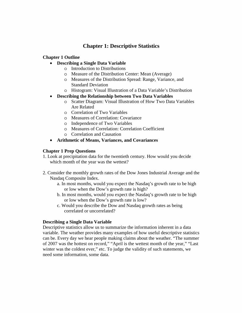
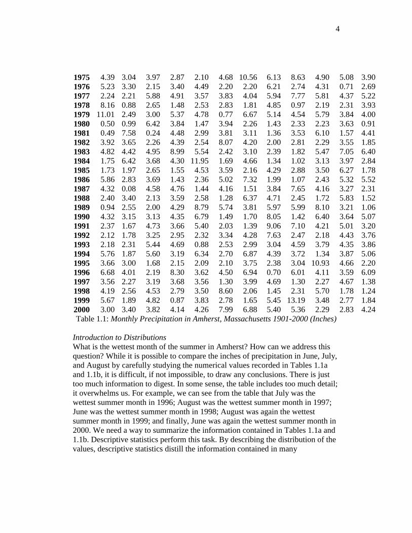
We shall focus our attention on precipitation in Amherst, Massachusetts during the twentieth century. Tables 1.1a and 1.1b report the inches of precipitation in Amherst for each month of the twentieth century.1 Amherst Precipitation Data: Monthly time series data of precipitation in Amherst, Massachusetts from January 1901 to December 2000.

Year Jan Feb Mar Apr May Jun Jul Aug Sep Oct Nov Dec 1901 2.09 0.56 5.66 5.80 5.12 0.75 3.77 5.75 3.67 4.17 1.30 8.51 1902 2.13 3.32 5.47 2.92 2.42 4.54 4.66 4.65 5.83 5.59 1.27 4.27 1903 3.28 4.27 6.40 2.30 0.48 7.79 4.64 4.92 1.66 2.72 2.04 3.95 1904 4.74 2.45 4.48 5.73 4.55 5.35 2.62 4.09 5.45 1.74 1.35 2.75 1905 3.90 1.70 3.66 2.56 1.28 2.86 2.63 6.47 6.26 2.27 2.06 3.15 1906 2.18 2.73 4.90 3.25 4.95 2.82 3.45 6.42 2.59 5.69 1.98 4.49 1907 2.73 1.92 1.82 1.98 4.02 2.61 3.87 1.44 8.74 5.00 4.50 3.89 1908 2.25 3.53 2.86 1.97 4.35 0.76 3.28 4.27 1.73 1.57 1.06 3.05 1909 3.56 5.16 3.01 5.53 3.36 2.24 2.24 3.80 4.99 1.23 1.06 2.95 1910 6.14 5.08 1.37 3.07 2.67 2.65 1.90 4.03 2.86 0.93 3.69 1.72 1911 2.36 2.18 3.80 1.87 1.37 2.02 4.21 5.92 3.41 8.81 3.84 4.42 1912 2.18 3.16 5.70 3.92 4.34 0.77 2.61 3.22 2.52 2.07 4.03 4.04 1913 3.98 2.94 6.30 3.30 4.94 0.90 1.59 2.26 2.56 5.16 2.11 3.38 1914 3.72 3.36 5.52 6.59 3.56 2.32 3.53 5.11 0.52 2.09 2.62 2.89 1915 6.52 7.02 0.12 3.99 1.20 3.00 9.13 8.28 1.37 2.89 2.20 5.86 1916 2.56 5.27 3.97 3.69 3.21 4.97 6.85 2.49 5.08 1.01 3.29 2.85 1917 3.30 1.98 4.08 1.83 4.13 5.27 3.36 7.06 2.42 6.60 0.63 2.56 1918 4.11 2.99 2.91 2.78 2.47 4.01 1.84 2.22 7.00 1.32 2.87 2.95 1919 2.02 2.80 4.22 2.37 6.20 1.09 4.17 4.80 4.45 1.81 6.20 1.48 1920 2.74 4.45 2.90 4.71 3.65 6.26 2.06 3.62 6.74 1.54 4.62 6.02 1921 2.00 2.38 3.57 6.47 4.56 3.87 6.00 2.35 1.84 1.08 6.20 1.90 1922 1.56 3.02 5.34 2.81 5.47 9.68 4.28 4.25 2.27 2.55 1.56 3.15 1923 6.02 1.81 1.98 3.19 3.26 2.24 1.77 2.55 1.89 5.50 5.05 4.23 1924 3.85 2.56 1.05 4.54 2.21 1.28 1.75 3.11 5.87 0.01 2.57 2.16 1925 3.42 3.64 4.12 3.10 2.55 4.28 6.97 1.93 3.09 4.74 3.23 3.56 1926 3.23 5.01 3.95 3.62 1.19 2.03 3.24 3.97 1.50 5.02 5.38 2.78 1927 2.50 2.62 1.96 1.60 4.83 3.37 3.40 5.01 2.79 4.59 8.65 5.66 1928 2.19 2.90 1.17 4.16 3.25 6.97 6.23 8.40 3.07 0.87 1.79 0.97 1929 4.33 3.92 3.20 6.89 4.17 3.06 0.70 1.54 3.62 2.75 2.73 4.05 1930 2.59 1.39 3.95 1.41 3.34 4.47 4.50 1.82 2.08 2.24 3.42 1.63 1931 3.58 1.80 3.79 2.95 7.44 4.24 3.87 6.57 2.50 3.06 1.55 3.83 1932 3.68 2.70 4.24 2.33 1.67 2.62 3.83 2.67 3.96 3.69 6.05 1.99 1933 2.44 3.48 4.79 5.03 1.69 3.68 2.25 6.63 12.34 3.90 1.19 2.81

3

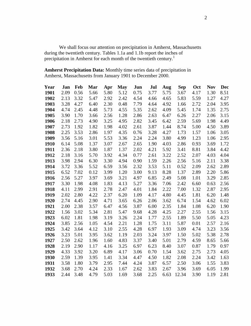
1934 3.50 2.82 3.60 4.44 3.42 4.67 1.73 3.02 9.54 2.35 3.50 2.99 1935 4.96 2.50 1.48 2.54 2.17 5.50 3.10 0.82 4.67 0.88 4.41 1.05 1936 6.47 2.64 7.04 4.07 1.76 3.28 1.45 4.85 3.80 4.80 2.02 5.96 1937 5.38 2.22 3.38 4.03 6.09 5.72 2.88 4.91 3.24 4.33 4.86 2.44 1938 6.60 1.77 2.00 3.07 3.81 8.45 7.45 2.04 14.55 2.49 3.02 3.95 1939 2.21 3.62 4.49 4.56 2.15 3.21 2.30 3.89 2.97 4.55 0.98 3.89 1940 2.63 2.72 5.58 6.37 5.67 2.46 4.69 1.56 1.53 1.04 6.31 3.01 1941 2.21 1.59 1.63 0.55 2.87 6.13 4.04 1.79 2.88 2.13 4.29 3.82 1942 3.54 1.66 7.89 0.96 2.98 3.63 4.95 2.93 3.94 3.27 6.07 6.03 1943 2.92 1.63 3.07 3.66 5.62 2.38 6.18 2.49 2.40 3.88 4.64 0.58 1944 1.24 2.34 4.36 3.66 1.35 4.70 3.88 4.33 5.31 1.74 4.21 2.18 1945 3.07 3.33 2.16 5.43 6.45 7.67 7.36 2.79 3.57 2.18 3.54 3.91 1946 2.72 3.52 1.60 2.16 5.41 3.30 5.30 4.00 4.88 1.51 0.70 3.51 1947 3.37 1.96 3.29 4.59 4.63 3.22 2.73 1.69 2.84 2.04 5.63 2.33 1948 2.63 2.45 2.92 2.87 5.83 5.67 2.95 3.56 1.92 1.14 5.22 2.87 1949 4.52 2.47 1.67 2.70 4.76 0.72 3.41 3.64 3.55 2.58 1.79 2.44 1950 4.33 3.99 2.67 3.64 2.77 3.65 2.83 2.93 2.24 1.87 6.60 4.64 1951 3.28 4.61 5.13 3.63 2.96 3.05 4.15 3.56 2.63 4.66 4.64 4.35 1952 4.02 1.97 3.17 3.40 4.00 4.97 4.99 3.98 4.05 1.07 0.89 4.10 1953 6.24 2.97 8.24 5.36 6.81 2.41 1.95 1.87 1.88 5.15 2.36 4.53 1954 2.45 1.94 3.93 4.24 4.80 2.68 3.00 3.91 6.14 1.89 5.07 3.19 1955 0.81 3.73 4.39 4.76 3.00 4.06 1.99 16.10 3.80 7.57 4.46 0.79 1956 1.75 3.52 4.94 4.49 2.02 2.86 2.90 2.71 5.55 1.64 3.10 4.83 1957 1.38 1.10 1.55 2.75 3.89 4.50 1.67 0.94 1.57 2.19 5.54 6.39 1958 4.03 2.21 2.62 4.58 2.98 1.64 5.13 5.19 3.90 3.79 3.79 1.57 1959 3.81 2.32 3.84 3.80 1.04 5.65 5.07 6.70 1.03 7.81 4.33 3.85 1960 2.35 3.90 3.32 4.30 3.44 4.73 6.84 3.74 6.75 2.43 3.13 2.71 1961 2.52 3.16 3.00 4.72 3.20 6.05 2.82 2.86 2.02 2.33 3.79 3.27 1962 3.01 3.59 1.84 2.69 2.03 1.06 2.16 3.33 3.74 4.16 2.11 3.30 1963 2.95 2.62 3.61 2.00 1.97 3.98 1.92 2.54 3.56 0.32 3.92 2.19 1964 5.18 2.32 2.71 2.72 0.83 1.84 3.02 3.01 0.94 1.32 1.68 3.98 1965 1.57 2.33 1.10 2.43 2.69 2.41 3.97 3.43 3.68 2.32 2.36 1.88 1966 1.72 3.43 2.93 1.28 2.26 3.30 5.83 0.67 5.14 4.51 3.48 2.22 1967 1.37 2.89 3.27 4.51 6.30 3.61 5.24 3.76 2.12 1.92 2.90 5.14 1968 1.87 1.02 4.47 2.62 3.02 7.19 0.73 1.12 2.64 3.10 5.78 5.08 1969 1.28 2.31 1.97 3.93 2.73 3.52 6.89 5.20 2.94 1.53 5.34 6.30 1970 0.66 3.55 3.52 3.69 4.16 4.97 2.17 5.23 3.05 2.45 3.27 2.37 1971 1.95 3.29 2.53 1.49 3.77 2.68 2.77 4.91 4.12 3.60 4.42 3.19 1972 1.86 3.47 4.85 4.06 4.72 10.25 2.42 2.25 1.84 2.51 6.92 6.81 1973 4.26 2.58 3.45 6.40 5.45 4.43 3.38 2.17 1.83 2.24 2.30 8.77 1974 3.35 2.42 4.34 2.61 5.21 3.40 3.71 3.97 7.29 1.94 2.76 3.67

4

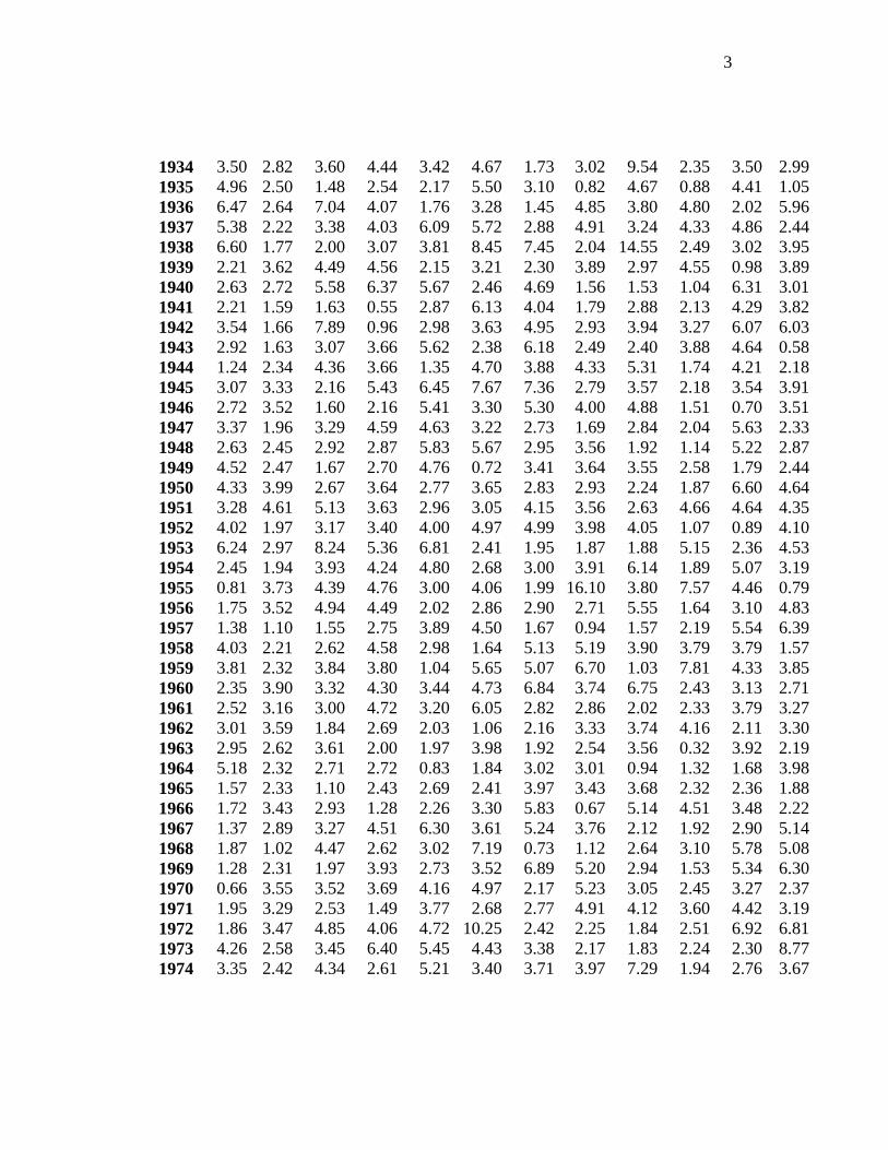
1975 4.39 3.04 3.97 2.87 2.10 4.68 10.56 6.13 8.63 4.90 5.08 3.90 1976 5.23 3.30 2.15 3.40 4.49 2.20 2.20 6.21 2.74 4.31 0.71 2.69 1977 2.24 2.21 5.88 4.91 3.57 3.83 4.04 5.94 7.77 5.81 4.37 5.22 1978 8.16 0.88 2.65 1.48 2.53 2.83 1.81 4.85 0.97 2.19 2.31 3.93 1979 11.01 2.49 3.00 5.37 4.78 0.77 6.67 5.14 4.54 5.79 3.84 4.00 1980 0.50 0.99 6.42 3.84 1.47 3.94 2.26 1.43 2.33 2.23 3.63 0.91 1981 0.49 7.58 0.24 4.48 2.99 3.81 3.11 1.36 3.53 6.10 1.57 4.41 1982 3.92 3.65 2.26 4.39 2.54 8.07 4.20 2.00 2.81 2.29 3.55 1.85 1983 4.82 4.42 4.95 8.99 5.54 2.42 3.10 2.39 1.82 5.47 7.05 6.40 1984 1.75 6.42 3.68 4.30 11.95 1.69 4.66 1.34 1.02 3.13 3.97 2.84 1985 1.73 1.97 2.65 1.55 4.53 3.59 2.16 4.29 2.88 3.50 6.27 1.78 1986 5.86 2.83 3.69 1.43 2.36 5.02 7.32 1.99 1.07 2.43 5.32 5.52 1987 4.32 0.08 4.58 4.76 1.44 4.16 1.51 3.84 7.65 4.16 3.27 2.31 1988 2.40 3.40 2.13 3.59 2.58 1.28 6.37 4.71 2.45 1.72 5.83 1.52 1989 0.94 2.55 2.00 4.29 8.79 5.74 3.81 5.97 5.99 8.10 3.21 1.06 1990 4.32 3.15 3.13 4.35 6.79 1.49 1.70 8.05 1.42 6.40 3.64 5.07 1991 2.37 1.67 4.73 3.66 5.40 2.03 1.39 9.06 7.10 4.21 5.01 3.20 1992 2.12 1.78 3.25 2.95 2.32 3.34 4.28 7.63 2.47 2.18 4.43 3.76 1993 2.18 2.31 5.44 4.69 0.88 2.53 2.99 3.04 4.59 3.79 4.35 3.86 1994 5.76 1.87 5.60 3.19 6.34 2.70 6.87 4.39 3.72 1.34 3.87 5.06 1995 3.66 3.00 1.68 2.15 2.09 2.10 3.75 2.38 3.04 10.93 4.66 2.20 1996 6.68 4.01 2.19 8.30 3.62 4.50 6.94 0.70 6.01 4.11 3.59 6.09 1997 3.56 2.27 3.19 3.68 3.56 1.30 3.99 4.69 1.30 2.27 4.67 1.38 1998 4.19 2.56 4.53 2.79 3.50 8.60 2.06 1.45 2.31 5.70 1.78 1.24 1999 5.67 1.89 4.82 0.87 3.83 2.78 1.65 5.45 13.19 3.48 2.77 1.84 2000 3.00 3.40 3.82 4.14 4.26 7.99 6.88 5.40 5.36 2.29 2.83 4.24 Table 1.1: Monthly Precipitation in Amherst, Massachusetts 1901-2000 (Inches)

Introduction to Distributions What is the wettest month of the summer in Amherst? How can we address this question? While it is possible to compare the inches of precipitation in June, July, and August by carefully studying the numerical values recorded in Tables 1.1a and 1.1b, it is difficult, if not impossible, to draw any conclusions. There is just too much information to digest. In some sense, the table includes too much detail; it overwhelms us. For example, we can see from the table that July was the wettest summer month in 1996; August was the wettest summer month in 1997; June was the wettest summer month in 1998; August was again the wettest summer month in 1999; and finally, June was again the wettest summer month in 2000. We need a way to summarize the information contained in Tables 1.1a and 1.1b. Descriptive statistics perform this task. By describing the distribution of the values, descriptive statistics distill the information contained in many

5

observations into single numbers. Summarizing data in this way has both benefits and costs. Without a summary we can easily “lose sight of the forest for the trees.” In the process of summarizing, however, some information will inevitably be lost.

First, we shall discuss the two most important types of descriptive

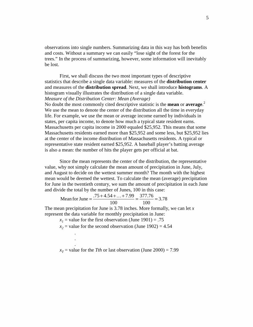
statistics that describe a single data variable: measures of the distribution center and measures of the distribution spread. Next, we shall introduce histograms. A histogram visually illustrates the distribution of a single data variable. Measure of the Distribution Center: Mean (Average) No doubt the most commonly cited descriptive statistic is the mean or average.2 We use the mean to denote the center of the distribution all the time in everyday life. For example, we use the mean or average income earned by individuals in states, per capita income, to denote how much a typical state resident earns. Massachusetts per capita income in 2000 equaled $25,952. This means that some Massachusetts residents earned more than $25,952 and some less, but $25,952 lies at the center of the income distribution of Massachusetts residents. A typical or representative state resident earned $25,952. A baseball player’s batting average is also a mean: the number of hits the player gets per official at bat.

Since the mean represents the center of the distribution, the representative

value, why not simply calculate the mean amount of precipitation in June, July, and August to decide on the wettest summer month? The month with the highest mean would be deemed the wettest. To calculate the mean (average) precipitation for June in the twentieth century, we sum the amount of precipitation in each June and divide the total by the number of Junes, 100 in this case:

.75 4.54 7.99 377.76Mean for June 3.78

100 100

+ + += = =…

The mean precipitation for June is 3.78 inches. More formally, we can let x represent the data variable for monthly precipitation in June:

x1 = value for the first observation (June 1901) = .75 x2 = value for the second observation (June 1902) = 4.54

.

.

. xT = value for the Tth or last observation (June 2000) = 7.99

6

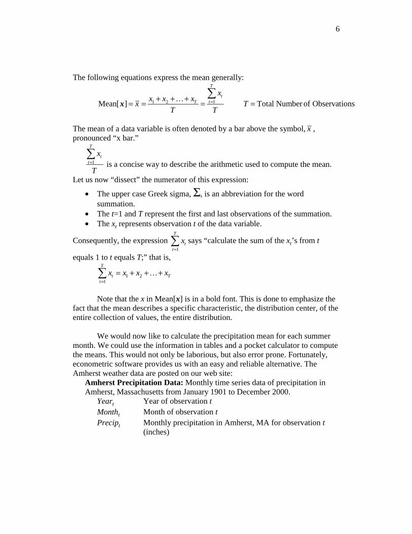
The following equations express the mean generally:

11 2Mean[ ] Total Number of Observations

T

ttT

xx x x

x TT T

=+ + += = = =∑

x…

The mean of a data variable is often denoted by a bar above the symbol, x , pronounced “x bar.”

1

T

tt

x

T=∑

is a concise way to describe the arithmetic used to compute the mean.

Let us now “dissect” the numerator of this expression:

• The upper case Greek sigma, Σ, is an abbreviation for the word summation.

• The t=1 and T represent the first and last observations of the summation. • The xt represents observation t of the data variable.

Consequently, the expression 1

T

tt

x=∑ says “calculate the sum of the xt’s from t

equals 1 to t equals T;” that is,

1 21

T

t Tt

x x x x=

= + + +∑ …

Note that the x in Mean[x] is in a bold font. This is done to emphasize the

fact that the mean describes a specific characteristic, the distribution center, of the entire collection of values, the entire distribution.

We would now like to calculate the precipitation mean for each summer

month. We could use the information in tables and a pocket calculator to compute the means. This would not only be laborious, but also error prone. Fortunately, econometric software provides us with an easy and reliable alternative. The Amherst weather data are posted on our web site:

Amherst Precipitation Data: Monthly time series data of precipitation in Amherst, Massachusetts from January 1901 to December 2000.

Yeart Year of observation t Montht Month of observation t Precipt Monthly precipitation in Amherst, MA for observation t

(inches)

7

Getting Started in EViews___________________________________________ Access the Amherst Weather Data online:

[Link to MIT-AmherstWeather-1901-2000.wf1 goes here.]

Then:

• In the File Download window: Click Open. (Note that different browsers may present you with a slightly different screen to open the workfile.)

Next, we instruct EViews to calculate the means: • In the Workfile window: Highlight year by clicking on it; then, while

depressing <Ctrl>, click on month and precip to highlight them also. • In the Workfile window: Double click on any of the highlighted variables. • A new list now pops up: Click Open Group. A spreadsheet including the

variables Year, Month, and Precip for all the months appears. • In the Group window: Click View; then click Descriptive Stats, and then

Individual Samples.3 Descriptive statistics for all the months of the twentieth century now appear. We only want to consider one month at a time. We want to compute the mean for June and then for July and then for August. Let us see how to do this.

• In the Group window: Click Sample. In the Sample window: Enter month=6 in the “If condition

(optional)” text area to restrict the sample to the sixth month, June, only.

Click OK. Descriptive statistics for the 100 Junes appear in the Group window. Record the mean.

• In the Group window: Click Sample. o In the Sample window: Enter month=7 in the “If condition

(optional)” text area to restrict the sample to July only. o Click OK. Descriptive statistics for the 100 Julys appear in the

Group window. Record the mean. • In the Group window: Click Sample.

o In the Sample window: Enter month=8 in the “If condition (optional)” text area to restrict the sample to August only.

o Click OK. Descriptive statistics for the 100 Augusts appear in the Group window. Record the mean.

• NB: This last step is critical. In the Group window: Click Sample. o In the Sample window: Clear the “If condition (optional)” text area

by deleting month=8; otherwise the restriction, month=8, will remain in effect if you ask EViews to perform any more computations.

8

Last, do not forget to close the file: • In the EViews window: Click File, then Exit. • In the Workfile window: Click No in response to the save changes made

to workfile. ________________________________________________________________ Table 1.2 summarizes the information. August has the highest mean. Based on the mean criterion, August was the wettest summer month in the twentieth century; the mean for August equals 3.96 which is greater than the mean for June or July.

Jun Jul Aug Mean 3.78 3.79 3.96

Table 1.2: Mean Monthly Precipitation for the Summer Months in Amherst, Massachusetts 1901-2000

Measures of the Distribution Spread: Range, Variance, and Standard Deviation While the center of the distribution is undoubtedly important, the spread can be crucial also. If the spread is small, all the values of the distribution lie close to the center, the mean. On the other hand, if the spread is large, some of the values lie far below the mean and some lie far about the mean. Farming provides a good illustration of why the spread can be important. Obviously, the mean precipitation during the growing season is critical to the farmer. But the spread of the precipitation is important also. Most crops grow best when they get a steady amount of moderate rain over the entire growing season. An unusually dry period followed by an unusually wet period or vice versa is not welcome news for the farmer. Both the center (mean) and the spread are important. The years 1951 and 1998 illustrate this well.

Year Apr May Jun Jul Aug Mean 1951 3.63 2.96 3.05 4.15 3.56 3.47 1998 2.79 3.50 8.60 2.06 1.45 3.68

Table 1.3: Growing Season Precipitation in Amherst, Massachusetts – 1951 and 1998

In reality, 1951 was a better growing season than 1998 even though the

mean for 1998 was a little higher. Precipitation was less volatile in 1951 than in 1998. Arguably the most straightforward measure of distribution spread is its range. In 1951, precipitation ranged from a minimum of 2.96 to a maximum of 4.15. In 1998, the range was larger from 1.45 to 8.60.

9

While the range is the simplest, it is not the most sensitive. The most widely cited measure of spread is the variance and its closely related cousin, the standard deviation. The variance equals the average of the squared deviations of the values from the mean. While this definition may sound a little overwhelming when first heard, it is not as daunting as it sounds. We can use the following three steps to calculate the variance:

• For each month, calculate the amount by which that month’s precipitation deviates from the mean.

• Square each month’s deviation. • Calculate the average of the squared deviations; that is, sum the squared

deviations and divide by the number of months, 5 in this case. Let us first calculate the variance for 1998:

Month Precipitation Mean Deviation From Mean Squared Deviation

Apr 2.79 3.68 2.79 – 3.68 = –0.89 0.7921 May 3.50 3.68 3.50 – 3.68 = –0.18 0.0324 Jun 8.60 3.68 8.60 – 3.68 = 4.92 24.2064 Jul 2.06 3.68 2.06 – 3.68 = –1.62 2.6244 Aug 1.45 3.68 1.45 – 3.68 = –2.23 4.9729

Sum of Squared Deviations = 32.6282 Sum of Squared Deviations 32.6282

Variance 6.52565N

= = =

Note that the mean and the variance are expressed in different units; the mean is expressed in inches and the variance in inches squared. Often it is useful to compare the mean and the measure of spread directly, in terms of the same units. The standard deviation allows us to do just that. The standard deviation is the square root of the variance; hence, the standard deviation is expressed in inches, just like the mean:

2Standard Deviation Variance 6.5256in 2.55in= = =

We can use the same procedure to calculate the variance and standard

deviation for 1951:

Month Precipitation Mean Deviation From Mean Squared Deviation

Apr 3.63 3.47 3.63 – 3.47 = 0.16 0.0256 May 2.96 3.47 2.96 – 3.47 = –0.51 0.2601 Jun 3.05 3.47 3.05 – 3.47 = –0.42 0.1764 Jul 4.15 3.47 4.15 – 3.47 = 0.68 0.4624 Aug 3.56 3.47 3.56 – 3.47 = 0.09 0.0081

Sum of Squared Deviations = 0.9326

10

Sum of Squared Deviations .9326Variance .1865

5N= = =

2Standard Deviation Variance .1865in .43in= = =

When the spread is small, as it was in 1951, all observations will be close

to the mean. Hence, the deviations will be small. The squared deviations, the variance, and the standard deviation will also be small. On the other hand, if the spread is large, as it was in 1998, some observations must be far from the mean. Hence, some deviations will be large. Some squared deviations, the variance, and the standard deviation will also be large. Let us summarize:

Spread small Spread large ↓ ↓

All deviations small Some deviations large ↓ ↓

All squared deviations small Some squared deviations large ↓ ↓

Variance small Variance large We can summarize the steps for calculating concisely with the following

equations: 2 2 2

1 2

2 2 21 2

( Mean[ ]) ( Mean[ ]) ( Mean[ ])Var[ ]

( ) ( ) ( )

where Total Number of Observations

Mean[ ] Mean of

T

T

x x x

T

x x x x x x

TT

x x

− + − + + −=

− + − + + −=

== =

x x xx

x

…

…

We can express the variance more concisely using “summation” notation:

2 2

1 1

( Mean[ ]) ( )Var[ ]

T T

t tt t

x x x

T T= =

− −= =∑ ∑x

x

The standard deviation is the square root of the variance:

SD[ ] Var[ ]=x x

11

Again, let us now “dissect” the summation expressions

2 2

1 1

( Mean[ ]) and ( )T T

t tt t

x x x= =

− −∑ ∑x :

• The upper case Greek sigma, Σ, is an abbreviation for the word summation.

• The t=1 and T represent the first and last observations of the summation. • The xt represents observation t of the data variable.

2 2

1 1

( Mean[ ]) and ( )T T

t tt t

x x x= =

− −∑ ∑x equal the sum of the squared deviations from the

mean. Note that the x in Var[x] and SD[x] is in a bold font. This emphasizes the

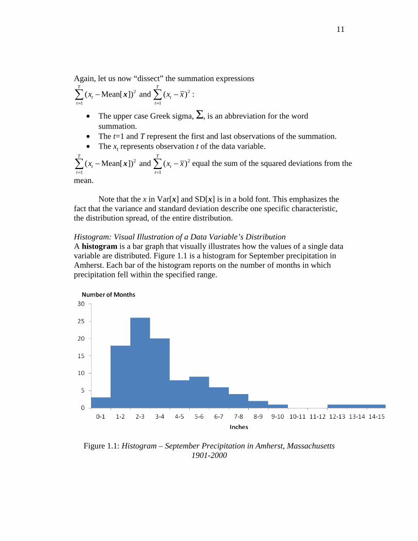
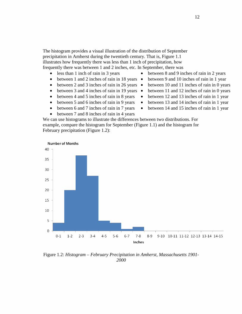
fact that the variance and standard deviation describe one specific characteristic, the distribution spread, of the entire distribution. Histogram: Visual Illustration of a Data Variable’s Distribution A histogram is a bar graph that visually illustrates how the values of a single data variable are distributed. Figure 1.1 is a histogram for September precipitation in Amherst. Each bar of the histogram reports on the number of months in which precipitation fell within the specified range.

Figure 1.1: Histogram – September Precipitation in Amherst, Massachusetts

1901-2000

12

The histogram provides a visual illustration of the distribution of September precipitation in Amherst during the twentieth century. That is, Figure 1.1 illustrates how frequently there was less than 1 inch of precipitation, how frequently there was between 1 and 2 inches, etc. In September, there was

• less than 1 inch of rain in 3 years • between 8 and 9 inches of rain in 2 years • between 1 and 2 inches of rain in 18 years • between 9 and 10 inches of rain in 1 year • between 2 and 3 inches of rain in 26 years • between 10 and 11 inches of rain in 0 years • between 3 and 4 inches of rain in 19 years • between 11 and 12 inches of rain in 0 years • between 4 and 5 inches of rain in 8 years • between 12 and 13 inches of rain in 1 year • between 5 and 6 inches of rain in 9 years • between 13 and 14 inches of rain in 1 year • between 6 and 7 inches of rain in 7 years • between 14 and 15 inches of rain in 1 year • between 7 and 8 inches of rain in 4 years

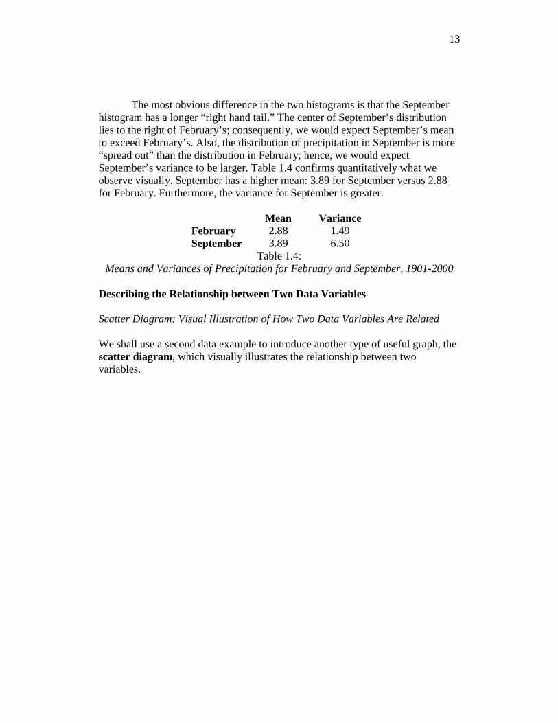
We can use histograms to illustrate the differences between two distributions. For example, compare the histogram for September (Figure 1.1) and the histogram for February precipitation (Figure 1.2):

Figure 1.2: Histogram – February Precipitation in Amherst, Massachusetts 1901-

2000

13

The most obvious difference in the two histograms is that the September histogram has a longer “right hand tail.” The center of September’s distribution lies to the right of February’s; consequently, we would expect September’s mean to exceed February’s. Also, the distribution of precipitation in September is more “spread out” than the distribution in February; hence, we would expect September’s variance to be larger. Table 1.4 confirms quantitatively what we observe visually. September has a higher mean: 3.89 for September versus 2.88 for February. Furthermore, the variance for September is greater.

Mean Variance February 2.88 1.49 September 3.89 6.50

Table 1.4: Means and Variances of Precipitation for February and September, 1901-2000

Describing the Relationship between Two Data Variables Scatter Diagram: Visual Illustration of How Two Data Variables Are Related We shall use a second data example to introduce another type of useful graph, the scatter diagram, which visually illustrates the relationship between two variables.

14

Stock Market Data: Monthly time series data for growth rates of the Dow Jones Industrial and Nasdaq stock indexes from January 1985 to December 2000.

Year Jan Feb Mar Apr May Jun Jul Aug Sep Oct Nov Dec1985 6.21 -0.22 -1.34 -0.69 4.55 1.53 0.90 -1.00 -0.40 3.44 7.12 5.071986 1.57 8.79 6.41 -1.90 5.20 0.85 -6.20 6.93 -6.89 6.23 1.94 -0.951987 13.82 3.06 3.63 -0.79 0.23 5.54 6.35 3.53 -2.50 -23.22 -8.02 5.741988 1.00 5.79 -4.03 2.22 -0.06 5.45 -0.61 -4.56 4.00 1.69 -1.59 2.561989 8.01 -3.58 1.56 5.46 2.54 -1.62 9.04 2.88 -1.63 -1.77 2.31 1.731990 -5.91 1.42 3.04 -1.86 8.28 0.14 0.85 -10.01 -6.19 -0.42 4.81 2.891991 3.90 5.33 1.10 -0.89 4.83 -3.99 4.06 0.62 -0.88 1.73 -5.68 9.471992 1.72 1.37 -0.99 3.82 1.13 -2.31 2.27 -4.02 0.44 -1.39 2.45 -0.121993 0.27 1.84 1.91 -0.22 2.91 -0.32 0.67 3.16 -2.63 3.53 0.09 1.901994 5.97 -3.68 -5.11 1.26 2.08 -3.55 3.85 3.96 -1.79 1.69 -4.32 2.551995 0.25 4.35 3.65 3.93 3.33 2.04 3.34 -2.08 3.87 -0.70 6.71 0.841996 5.44 1.67 1.85 -0.32 1.33 0.20 -2.22 1.58 4.74 2.50 8.16 -1.131997 5.66 0.95 -4.28 6.46 4.59 4.66 7.17 -7.30 4.24 -6.33 5.12 1.091998 -0.02 8.08 2.97 3.00 -1.80 0.58 -0.77 -15.13 4.03 9.56 6.10 0.711999 1.93 -0.56 5.15 10.25 -2.13 3.89 -2.88 1.63 -4.55 3.80 1.38 5.692000 -4.84 -7.42 7.84 -1.72 -1.97 -0.71 0.71 6.59 -5.03 3.01 -5.07 3.59

Table 1.5a: Monthly Percentage Growth Rate of Dow Jones Industrial Index

Year Jan Feb Mar Apr May Jun Jul Aug Sep Oct Nov Dec1985 12.79 1.97 -1.76 0.50 3.64 1.86 1.72 -1.19 -5.84 4.35 7.35 3.471986 3.35 7.06 4.23 2.27 4.44 1.32 -8.41 3.10 -8.41 2.88 -0.33 -3.001987 12.41 8.39 1.20 -2.86 -0.31 1.97 2.40 4.62 -2.35 -27.23 -5.60 8.291988 4.30 6.47 2.07 1.23 -2.35 6.59 -1.87 -2.76 2.95 -1.34 -2.88 2.661989 5.22 -0.40 1.75 5.14 4.35 -2.44 4.25 3.42 0.77 -3.66 0.11 -0.291990 -8.58 2.41 2.28 -3.54 9.26 0.72 -5.21 -13.01 -9.63 -4.27 8.88 4.091991 10.81 9.39 6.44 0.50 4.41 -5.97 5.49 4.71 0.23 3.06 -3.51 11.921992 5.78 2.14 -4.69 -4.16 1.15 -3.71 3.06 -3.05 3.58 3.75 7.86 3.711993 2.86 -3.67 2.89 -4.16 5.91 0.49 0.11 5.41 2.68 2.16 -3.19 2.971994 3.05 -1.00 -6.19 -1.29 0.18 -3.98 2.29 6.02 -0.17 1.73 -3.49 0.221995 0.43 5.10 2.96 3.28 2.44 7.97 7.26 1.89 2.30 -0.72 2.23 -0.671996 0.73 3.80 0.12 8.09 4.44 -4.70 -8.81 5.64 7.48 -0.44 5.82 -0.121997 6.88 -5.13 -6.67 3.20 11.07 2.98 10.52 -0.41 6.20 -5.46 0.44 -1.891998 3.12 9.33 3.68 1.78 -4.79 6.51 -1.18 -19.93 12.98 4.58 10.06 12.471999 14.28 -8.69 7.58 3.31 -2.84 8.73 -1.77 3.82 0.25 8.02 12.46 21.982000 -3.17 19.19 -2.64 -15.57 -11.91 16.62 -5.02 11.66 -12.68 -8.25 -22.90 -4.90

Table 1.5b: Monthly Percentage Growth Rate of Nasdaq Index

15

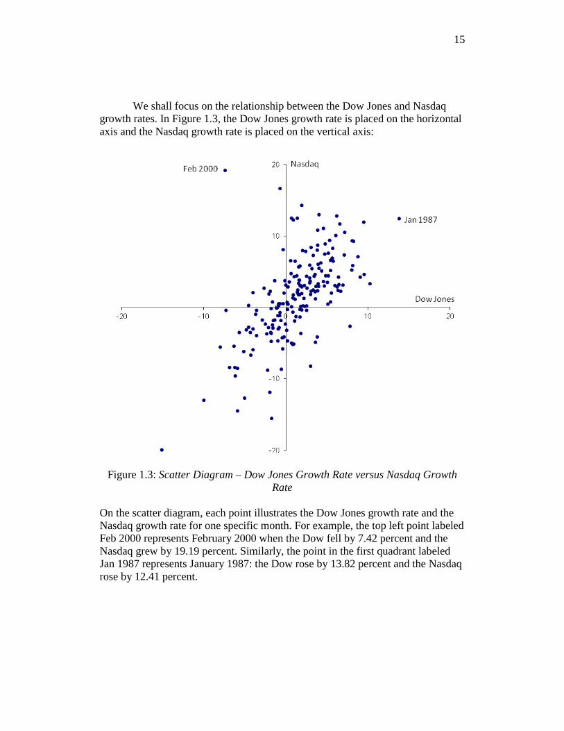
We shall focus on the relationship between the Dow Jones and Nasdaq growth rates. In Figure 1.3, the Dow Jones growth rate is placed on the horizontal axis and the Nasdaq growth rate is placed on the vertical axis:

Figure 1.3: Scatter Diagram – Dow Jones Growth Rate versus Nasdaq Growth

Rate

On the scatter diagram, each point illustrates the Dow Jones growth rate and the Nasdaq growth rate for one specific month. For example, the top left point labeled Feb 2000 represents February 2000 when the Dow fell by 7.42 percent and the Nasdaq grew by 19.19 percent. Similarly, the point in the first quadrant labeled Jan 1987 represents January 1987: the Dow rose by 13.82 percent and the Nasdaq rose by 12.41 percent.

16

Correlation of Two Variables The Dow Jones and Nasdaq growth rates appear to be correlated. Two variables are correlated when information about one variable helps us predict the other. Typically, when the Dow Jones growth rate is positive, the Nasdaq growth rate is also positive; similarly, when the Dow Jones growth rate is negative, the Nasdaq growth rate is usually negative. Although there are exceptions, February 2000 for example, knowing one growth rate typically helps us predict the other. For example, if we knew that the Dow Jones growth rate was positive in one specific month, we would predict that the Nasdaq growth rate would be positive also. While we would not always be correct, we would be right most of the time. Measure of Correlation: Covariance Covariance quantifies the notion of correlation. We can use the following three steps to calculate the covariance of two data variables, x and y:

• For each observation, calculate the amount by which variable x deviates from its mean and the amount by which variable y deviates from its mean.

• Multiply each observation’s x deviation by its y deviation. • Calculate the average of these products; that is, sum the products of the

deviations and divide by the number of observations. We can express these steps concisely with an equation:

( )( ) ( )( ) ( )( )

( )( )

1 1 2 2

1

Cov[ , ]

where Total Number of Observations

Mean[ ] Mean of

Mean[ ] Mean of

T T

T

t tt

x x y y x x y y x x y y

T

x x y y

TT

x x

y y

=

− − + − − + + − −=

− −=

== == =

∑

x y

x

y

…

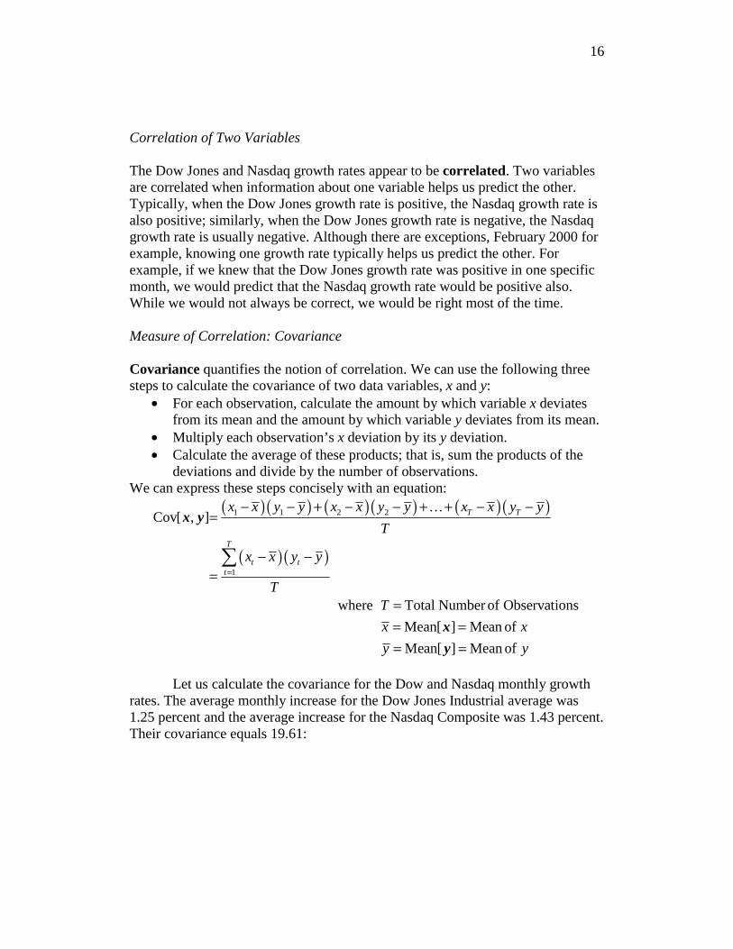
Let us calculate the covariance for the Dow and Nasdaq monthly growth

rates. The average monthly increase for the Dow Jones Industrial average was 1.25 percent and the average increase for the Nasdaq Composite was 1.43 percent. Their covariance equals 19.61:

17

( )( ) ( )( ) ( )( )

( ) ( ) ( ) ( ) ( ) ( )

1 1 2 2Cov[ , ]

6.21 1.25 12.79 1.43 .22 1.25 1.97 1.43 3.59 1.25 4.90 1.43

19219.61

T Tx x y y x x y y x x y y

T

− − + − − + + − −=

− − + − − − + + − − −=

=

x y…

…

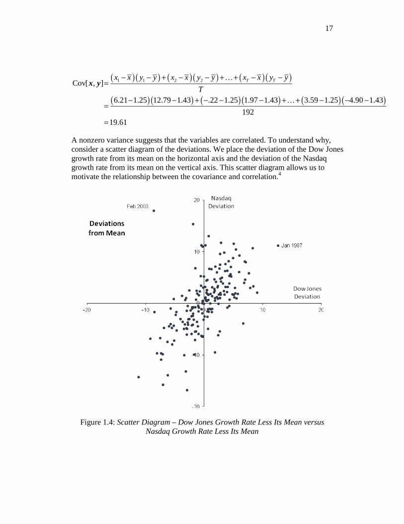
A nonzero variance suggests that the variables are correlated. To understand why, consider a scatter diagram of the deviations. We place the deviation of the Dow Jones growth rate from its mean on the horizontal axis and the deviation of the Nasdaq growth rate from its mean on the vertical axis. This scatter diagram allows us to motivate the relationship between the covariance and correlation.4

Figure 1.4: Scatter Diagram – Dow Jones Growth Rate Less Its Mean versus

Nasdaq Growth Rate Less Its Mean

18

The covariance equation and the scatter diagram are related. The numerator of the covariance equation equals the sum of the products of each month’s deviations, ( )( )t tx x y y− − :

( )( )1Cov[ , ]

T

t tt

x x y y

T=

− −=∑

x y

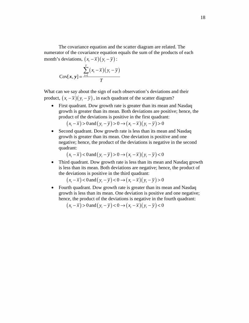
What can we say about the sign of each observation’s deviations and their product, ( )( )t tx x y y− − , in each quadrant of the scatter diagram?

• First quadrant. Dow growth rate is greater than its mean and Nasdaq growth is greater than its mean. Both deviations are positive; hence, the product of the deviations is positive in the first quadrant:

( ) ( ) ( )( )0and 0 0t t t tx x y y x x y y− > − > → − − >

• Second quadrant. Dow growth rate is less than its mean and Nasdaq growth is greater than its mean. One deviation is positive and one negative; hence, the product of the deviations is negative in the second quadrant:

( ) ( ) ( )( )0and 0 0t t t tx x y y x x y y− < − > → − − <

• Third quadrant. Dow growth rate is less than its mean and Nasdaq growth is less than its mean. Both deviations are negative; hence, the product of the deviations is positive in the third quadrant:

( ) ( ) ( )( )0and 0 0t t t tx x y y x x y y− < − < → − − >

• Fourth quadrant. Dow growth rate is greater than its mean and Nasdaq growth is less than its mean. One deviation is positive and one negative; hence, the product of the deviations is negative in the fourth quadrant:

( ) ( ) ( )( )0and 0 0t t t tx x y y x x y y− > − < → − − <

19

(xt−x−)(yt−y

−) > 0

(xt-x−)(yt-y

−) > 0

(xt−x−)(yt−y

−) < 0

(xt−x−)(yt−y

−) < 0

(xt - x−)

(yt − y−)

(xt−x−)>0 (yt−y

−)>0(xt−x−)<0 (yt−y

−)>0

(xt−x−)<0 (yt−y

−)<0 (xt−x−)>0 (yt−y

−)<0

Quadrant IQuadrant II

Quadrant III Quadrant IV

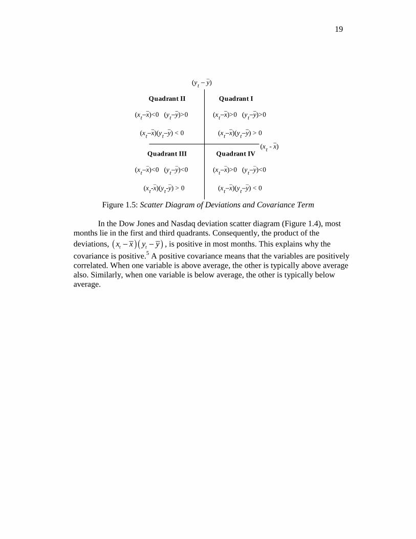
Figure 1.5: Scatter Diagram of Deviations and Covariance Term

In the Dow Jones and Nasdaq deviation scatter diagram (Figure 1.4), most

months lie in the first and third quadrants. Consequently, the product of the deviations, ( )( )t tx x y y− − , is positive in most months. This explains why the

covariance is positive.5 A positive covariance means that the variables are positively correlated. When one variable is above average, the other is typically above average also. Similarly, when one variable is below average, the other is typically below average.

20

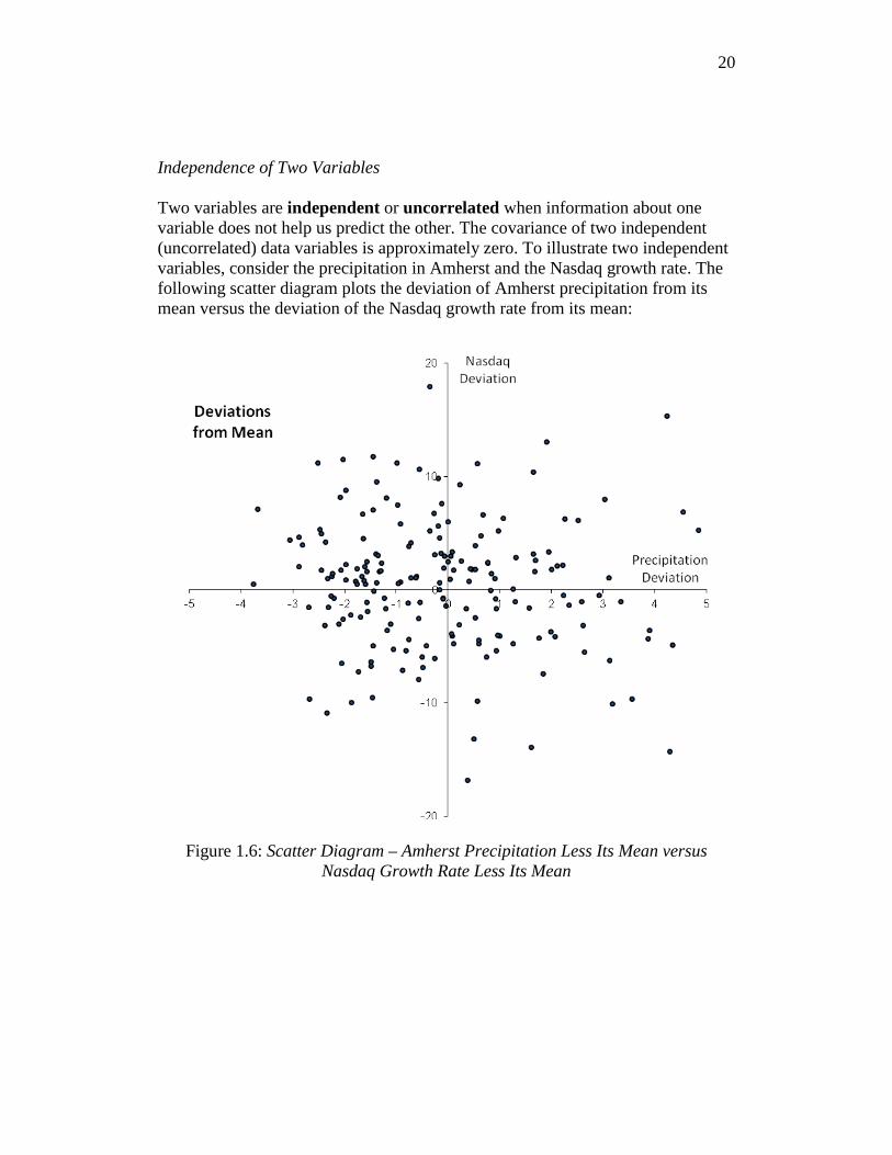
Independence of Two Variables Two variables are independent or uncorrelated when information about one variable does not help us predict the other. The covariance of two independent (uncorrelated) data variables is approximately zero. To illustrate two independent variables, consider the precipitation in Amherst and the Nasdaq growth rate. The following scatter diagram plots the deviation of Amherst precipitation from its mean versus the deviation of the Nasdaq growth rate from its mean:

Figure 1.6: Scatter Diagram – Amherst Precipitation Less Its Mean versus

Nasdaq Growth Rate Less Its Mean

21

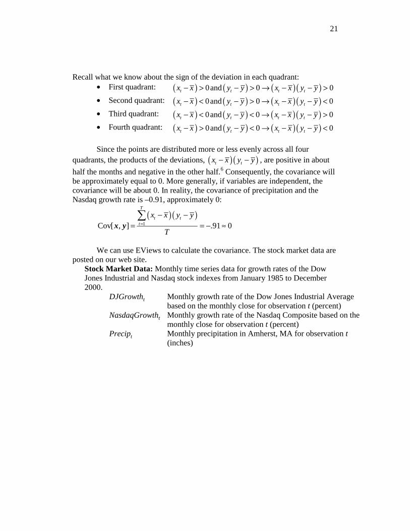
Recall what we know about the sign of the deviation in each quadrant: • First quadrant: ( ) ( ) ( )( )0and 0 0t t t tx x y y x x y y− > − > → − − >

• Second quadrant: ( ) ( ) ( )( )0and 0 0t t t tx x y y x x y y− < − > → − − <

• Third quadrant: ( ) ( ) ( )( )0and 0 0t t t tx x y y x x y y− < − < → − − >

• Fourth quadrant: ( ) ( ) ( )( )0and 0 0t t t tx x y y x x y y− > − < → − − <

Since the points are distributed more or less evenly across all four

quadrants, the products of the deviations, ( )( )t tx x y y− − , are positive in about

half the months and negative in the other half.6 Consequently, the covariance will be approximately equal to 0. More generally, if variables are independent, the covariance will be about 0. In reality, the covariance of precipitation and the Nasdaq growth rate is –0.91, approximately 0:

( )( )1Cov[ , ] .91 0

T

t tt

x x y y

T=

− −= = − ≈∑

x y

We can use EViews to calculate the covariance. The stock market data are

posted on our web site. Stock Market Data: Monthly time series data for growth rates of the Dow Jones Industrial and Nasdaq stock indexes from January 1985 to December 2000.

DJGrowtht Monthly growth rate of the Dow Jones Industrial Average based on the monthly close for observation t (percent)

NasdaqGrowtht Monthly growth rate of the Nasdaq Composite based on the monthly close for observation t (percent)

Precipt Monthly precipitation in Amherst, MA for observation t (inches)

22

Getting Started in EViews___________________________________________ Access the Stock Market Data online:

[Link to MIT-StockMarket-1985-2000.wf1 goes here.]

Then:

• In the File Download window: Click Open. (Note that different browsers may present you with a slightly different screen to open the workfile.)

Next, we instruct EViews to calculate the covariance of Amherst precipitation and the Nasdaq growth rate:

• In the Workfile window: Highlight precip by clicking on it; then while depressing <Ctrl> click on nasdaqgrowth to highlight it.

• In the Workfile window: Double click on any of the highlighted variables. • A new list now pops up: Click Open Group. A spreadsheet including the

variables Precip and NasdaqGrowth appears. • In the Group window: Click View, and then click Covariance Analysis… • In the Covariance Analysis window: Be certain that the Covariance

checkbox is selected; then, click OK. Last, close the file:

• In the EViews window: Click File, then Exit. • In the Workfile window: Click No in response to the save changes made

to the workfile. __________________________________________________________________

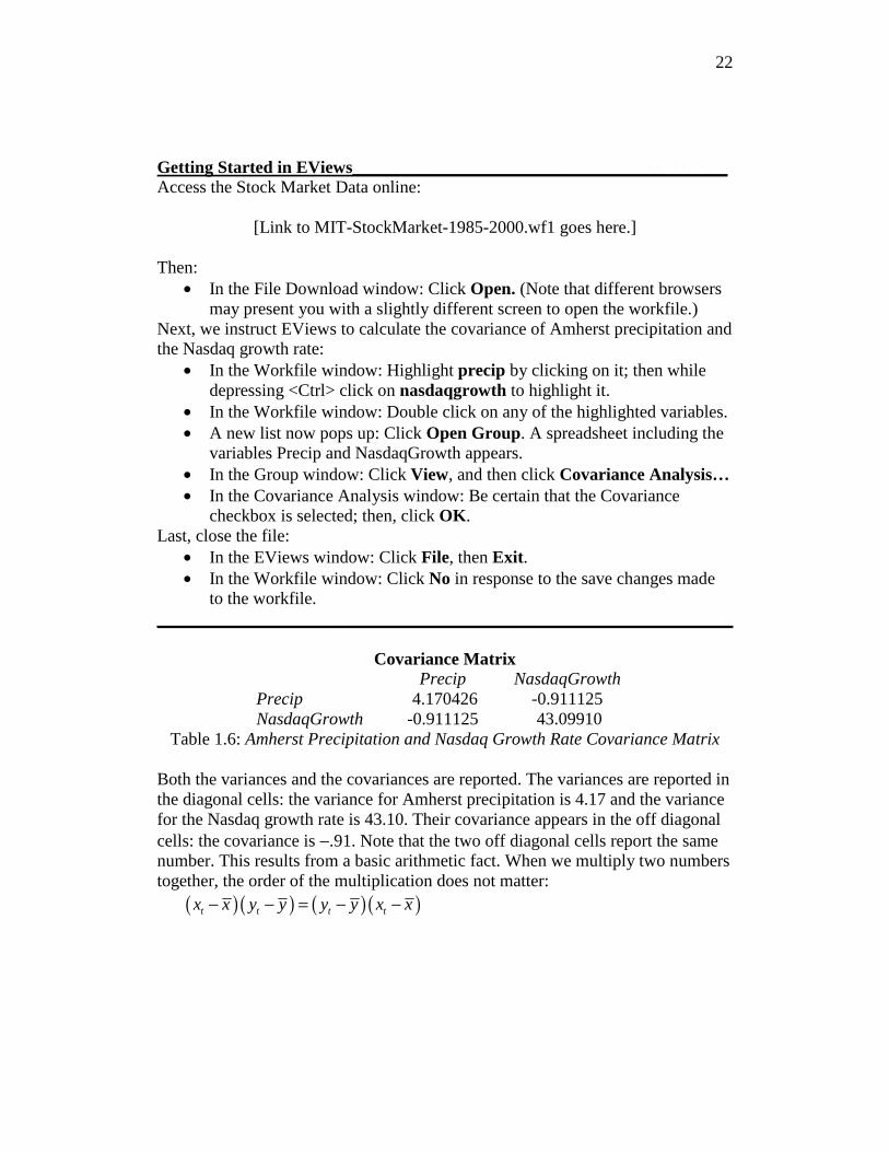
Covariance Matrix

Precip NasdaqGrowth

Precip 4.170426 -0.911125 NasdaqGrowth -0.911125 43.09910

Table 1.6: Amherst Precipitation and Nasdaq Growth Rate Covariance Matrix

Both the variances and the covariances are reported. The variances are reported in the diagonal cells: the variance for Amherst precipitation is 4.17 and the variance for the Nasdaq growth rate is 43.10. Their covariance appears in the off diagonal cells: the covariance is −.91. Note that the two off diagonal cells report the same number. This results from a basic arithmetic fact. When we multiply two numbers together, the order of the multiplication does not matter:

( )( ) ( )( )t t t tx x y y y y x x− − = − −

23

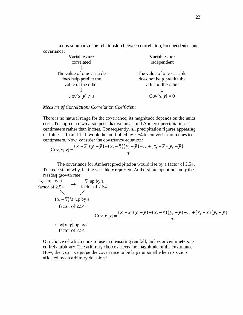
Let us summarize the relationship between correlation, independence, and covariance:

Variables are Variables are correlated independent

↓ ↓ The value of one variable The value of one variable

does help predict the does not help predict the value of the other value of the other

↓ ↓ Cov[x, y] ≠ 0 Cov[x, y] = 0

Measure of Correlation: Correlation Coefficient There is no natural range for the covariance; its magnitude depends on the units used. To appreciate why, suppose that we measured Amherst precipitation in centimeters rather than inches. Consequently, all precipitation figures appearing in Tables 1.1a and 1.1b would be multiplied by 2.54 to convert from inches to centimeters. Now, consider the covariance equation:

( )( ) ( ) ( ) ( ) ( )1 1 2 2Cov[ , ] T Tx x y y x x y y x x y y

T

− − + − − + + − −=x y

…

The covariance for Amherst precipitation would rise by a factor of 2.54.

To understand why, let the variable x represent Amherst precipitation and y the Nasdaq growth rate:

xt’s up by a factor of 2.54

→ x up by a

factor of 2.54

é ã ( ) 'tx x s− up by a

factor of 2.54

⏐ ⏐ ↓

( )( ) ( ) ( ) ( ) ( )1 1 2 2Cov[ , ] T Tx x y y x x y y x x y y

T

− − + − − + + − −=x y

…

Cov[x, y] up by a factor of 2.54

Our choice of which units to use in measuring rainfall, inches or centimeters, is entirely arbitrary. The arbitrary choice affects the magnitude of the covariance. How, then, can we judge the covariance to be large or small when its size is affected by an arbitrary decision?

24

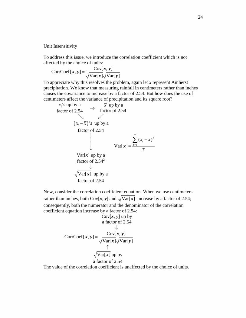
Unit Insensitivity To address this issue, we introduce the correlation coefficient which is not affected by the choice of units:

Cov[ , ]CorrCoef[ , ]

Var[ ] Var[ ]= x y

x yx y

To appreciate why this resolves the problem, again let x represent Amherst precipitation. We know that measuring rainfall in centimeters rather than inches causes the covariance to increase by a factor of 2.54. But how does the use of centimeters affect the variance of precipitation and its square root?

xt’s up by a factor of 2.54

→ x up by a

factor of 2.54

é ã ( ) 'tx x s− up by a

factor of 2.54

⏐ ⏐ ⏐ ↓

2

1

( )Var[ ]

T

tt

x x

T=

−=∑

x

Var[x] up by a factor of 2.542

↓ Var[ ]x up by a

factor of 2.54

Now, consider the correlation coefficient equation. When we use centimeters

rather than inches, both Cov[x, y] and Var[ ]x increase by a factor of 2.54;

consequently, both the numerator and the denominator of the correlation coefficient equation increase by a factor of 2.54:

Cov[x, y] up by a factor of 2.54

↓ Cov[ , ]

CorrCoef[ , ]Var[ ] Var[ ]

= x yx y

x y

↑ Var[ ]x up by

a factor of 2.54 The value of the correlation coefficient is unaffected by the choice of units.

25

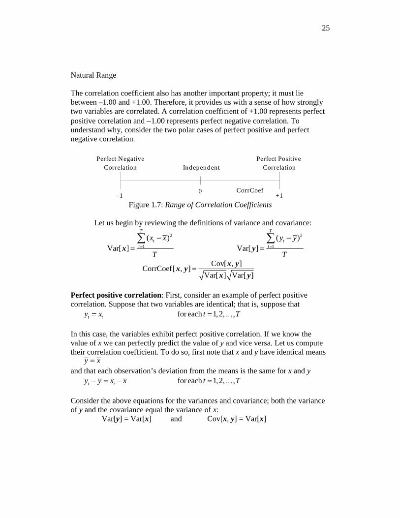
Natural Range The correlation coefficient also has another important property; it must lie between –1.00 and +1.00. Therefore, it provides us with a sense of how strongly two variables are correlated. A correlation coefficient of +1.00 represents perfect positive correlation and −1.00 represents perfect negative correlation. To understand why, consider the two polar cases of perfect positive and perfect negative correlation.

−1 +1

Perfect PositiveCorrelation

Perfect NegativeCorrelationIndependent

CorrCoef0

Figure 1.7: Range of Correlation Coefficients

Let us begin by reviewing the definitions of variance and covariance:

2 2

1 1

( ) ( )Var[ ] Var[ ]

T T

t tt t

x x y y

T T= =

− −= =∑ ∑

x y

Cov[ , ]CorrCoef[ , ]

Var[ ] Var[ ]= x y

x yx y

Perfect positive correlation: First, consider an example of perfect positive correlation. Suppose that two variables are identical; that is, suppose that

for each 1,2, ,t ty x t T= = …

In this case, the variables exhibit perfect positive correlation. If we know the value of x we can perfectly predict the value of y and vice versa. Let us compute their correlation coefficient. To do so, first note that x and y have identical means

y x= and that each observation’s deviation from the means is the same for x and y

for each 1,2, ,t ty y x x t T− = − = …

Consider the above equations for the variances and covariance; both the variance of y and the covariance equal the variance of x:

Var[y] = Var[x] and Cov[x, y] = Var[x]

26

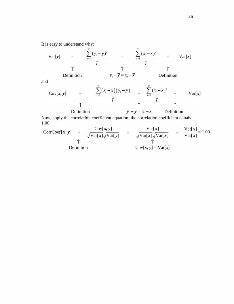
It is easy to understand why:

Var[y] = 2

1

( )T

tt

y y

T=

−∑

= 2

1

( )T

tt

x x

T=

−∑

= Var[x]

↑ ↑ ↑ Definition t ty y x x− = − Definition

and

Cov[x, y] = ( )( )

1

T

t tt

x x y y

T=

− −∑

= 2

1

( )T

tt

x x

T=

−∑

= Var[x]

↑ ↑ ↑ Definition t ty y x x− = − Definition

Now, apply the correlation coefficient equation; the correlation coefficient equals 1.00:

CorrCoef[ , ]x y = Cov[ ]

Var[ ] Var[ ]

x, y

x y =

Var[ ]

Var[ ] Var[ ]

x

x x =

Var[ ]

Var[ ]

xx

= 1.00

↑ ↑ Definition Cov[x, y] = Var[x]

27

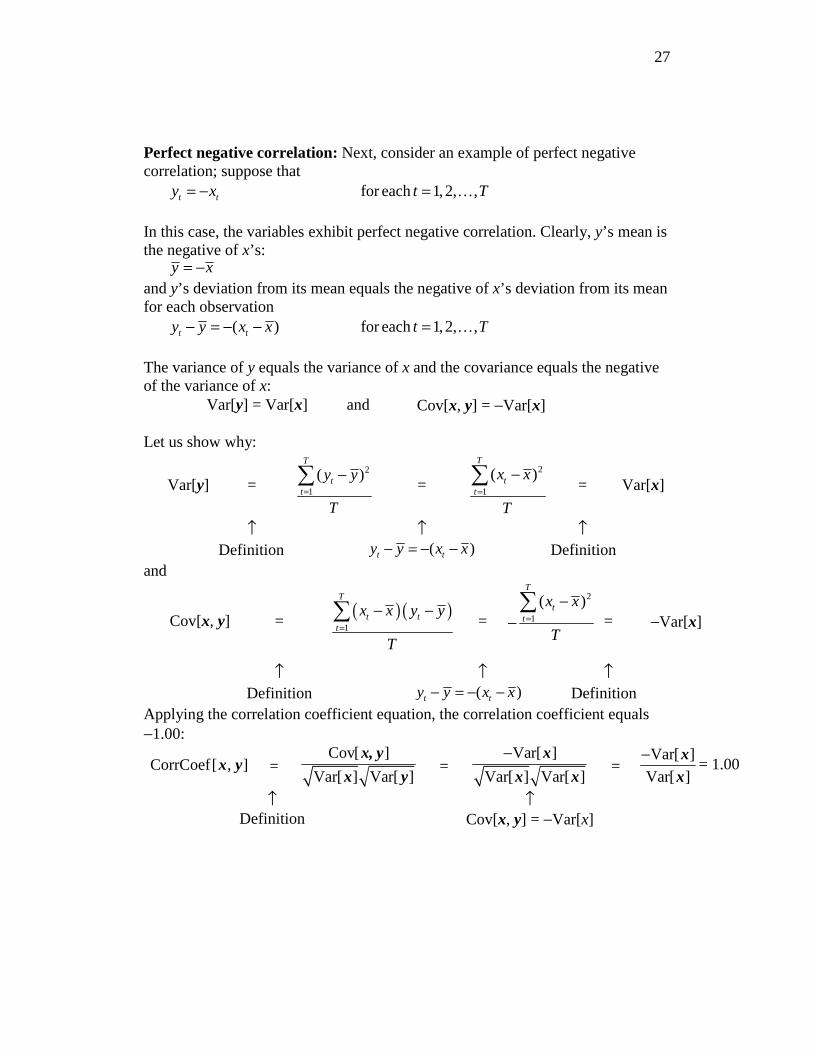
Perfect negative correlation: Next, consider an example of perfect negative correlation; suppose that

for each 1,2, ,t ty x t T= − = …

In this case, the variables exhibit perfect negative correlation. Clearly, y’s mean is the negative of x’s:

y x= − and y’s deviation from its mean equals the negative of x’s deviation from its mean for each observation

( ) for each 1,2, ,t ty y x x t T− = − − = …

The variance of y equals the variance of x and the covariance equals the negative of the variance of x:

Var[y] = Var[x] and Cov[x, y] = −Var[x] Let us show why:

Var[y] = 2

1

( )T

tt

y y

T=

−∑

= 2

1

( )T

tt

x x

T=

−∑

= Var[x]

↑ ↑ ↑ Definition ( )t ty y x x− = − − Definition

and

Cov[x, y] = ( )( )

1

T

t tt

x x y y

T=

− −∑

=

2

1

( )T

tt

x x

T=

−−∑

= −Var[x]

↑ ↑ ↑ Definition ( )t ty y x x− = − − Definition

Applying the correlation coefficient equation, the correlation coefficient equals −1.00:

CorrCoef[ , ]x y = Cov[ ]

Var[ ] Var[ ]

x, y

x y =

Var[ ]

Var[ ] Var[ ]

− x

x x =

Var[ ]

Var[ ]

− xx

= 1.00

↑ ↑ Definition Cov[x, y] = −Var[x]

28

Getting Started in EViews___________________________________________ Access the Stock Market Data online:

[Link to MIT-StockMarket-1985-2000.wf1 goes here.]

Then:

• In the File Download window: Click Open. (Note that different browsers may present you with a slightly different screen to open the workfile.)

• In the Workfile window: Highlight precip by clicking on it; then, while depressing <Ctrl>, click on nasdaqgrowth and djgrowth to highlight them also.

• In the Workfile window: Double click on any of the highlighted variables. • A new list now pops up: Click Open Group. A spreadsheet including the

variables Precip, NasdaqGrowth, and DJGrowth appears. • In the Group window: Click View, and then click Covariance Analysis… • In the Covariance Analysis window: Clear the Covariance box and Select

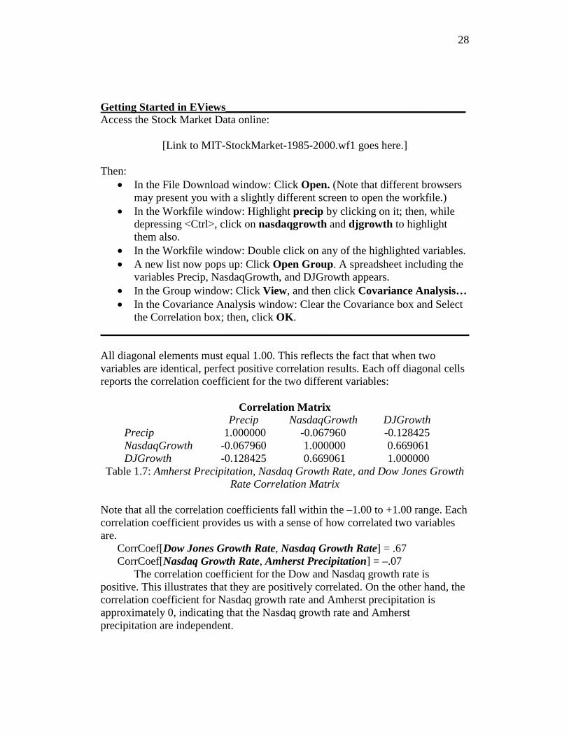
the Correlation box; then, click OK. __________________________________________________________________ All diagonal elements must equal 1.00. This reflects the fact that when two variables are identical, perfect positive correlation results. Each off diagonal cells reports the correlation coefficient for the two different variables:

Correlation Matrix

Precip NasdaqGrowth DJGrowth

Precip 1.000000 -0.067960 -0.128425 NasdaqGrowth -0.067960 1.000000 0.669061 DJGrowth -0.128425 0.669061 1.000000

Table 1.7: Amherst Precipitation, Nasdaq Growth Rate, and Dow Jones Growth Rate Correlation Matrix

Note that all the correlation coefficients fall within the –1.00 to +1.00 range. Each correlation coefficient provides us with a sense of how correlated two variables are.

CorrCoef[Dow Jones Growth Rate, Nasdaq Growth Rate] = .67 CorrCoef[Nasdaq Growth Rate, Amherst Precipitation] = –.07

The correlation coefficient for the Dow and Nasdaq growth rate is positive. This illustrates that they are positively correlated. On the other hand, the correlation coefficient for Nasdaq growth rate and Amherst precipitation is approximately 0, indicating that the Nasdaq growth rate and Amherst precipitation are independent.

29

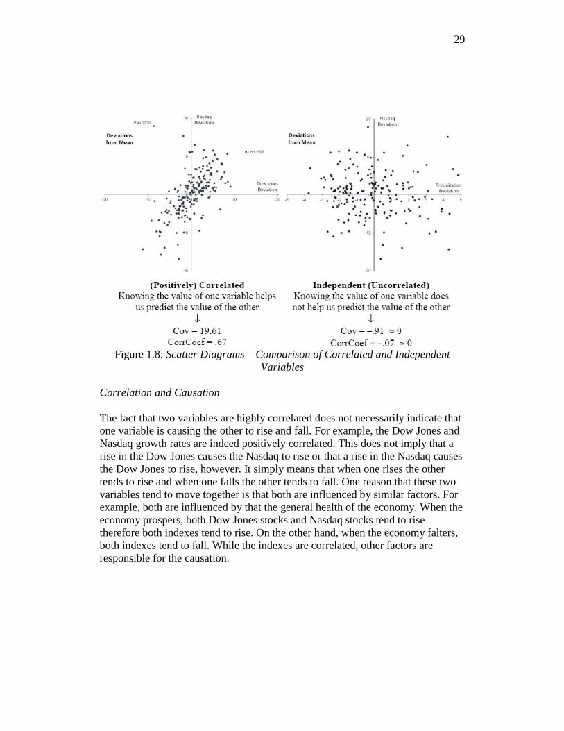
Figure 1.8: Scatter Diagrams – Comparison of Correlated and Independent

Variables

Correlation and Causation The fact that two variables are highly correlated does not necessarily indicate that one variable is causing the other to rise and fall. For example, the Dow Jones and Nasdaq growth rates are indeed positively correlated. This does not imply that a rise in the Dow Jones causes the Nasdaq to rise or that a rise in the Nasdaq causes the Dow Jones to rise, however. It simply means that when one rises the other tends to rise and when one falls the other tends to fall. One reason that these two variables tend to move together is that both are influenced by similar factors. For example, both are influenced by that the general health of the economy. When the economy prospers, both Dow Jones stocks and Nasdaq stocks tend to rise therefore both indexes tend to rise. On the other hand, when the economy falters, both indexes tend to fall. While the indexes are correlated, other factors are responsible for the causation.

30

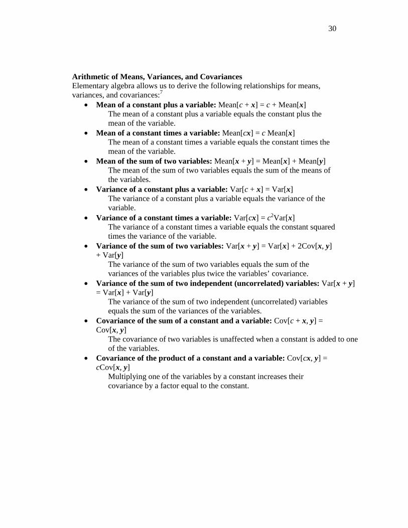
Arithmetic of Means, Variances, and Covariances Elementary algebra allows us to derive the following relationships for means, variances, and covariances:7

• Mean of a constant plus a variable: Mean[c + x] = c + Mean[x] The mean of a constant plus a variable equals the constant plus the mean of the variable.

• Mean of a constant times a variable: Mean[cx] = c Mean[x] The mean of a constant times a variable equals the constant times the mean of the variable.

• Mean of the sum of two variables: Mean[x + y] = Mean[x] + Mean[y] The mean of the sum of two variables equals the sum of the means of the variables.

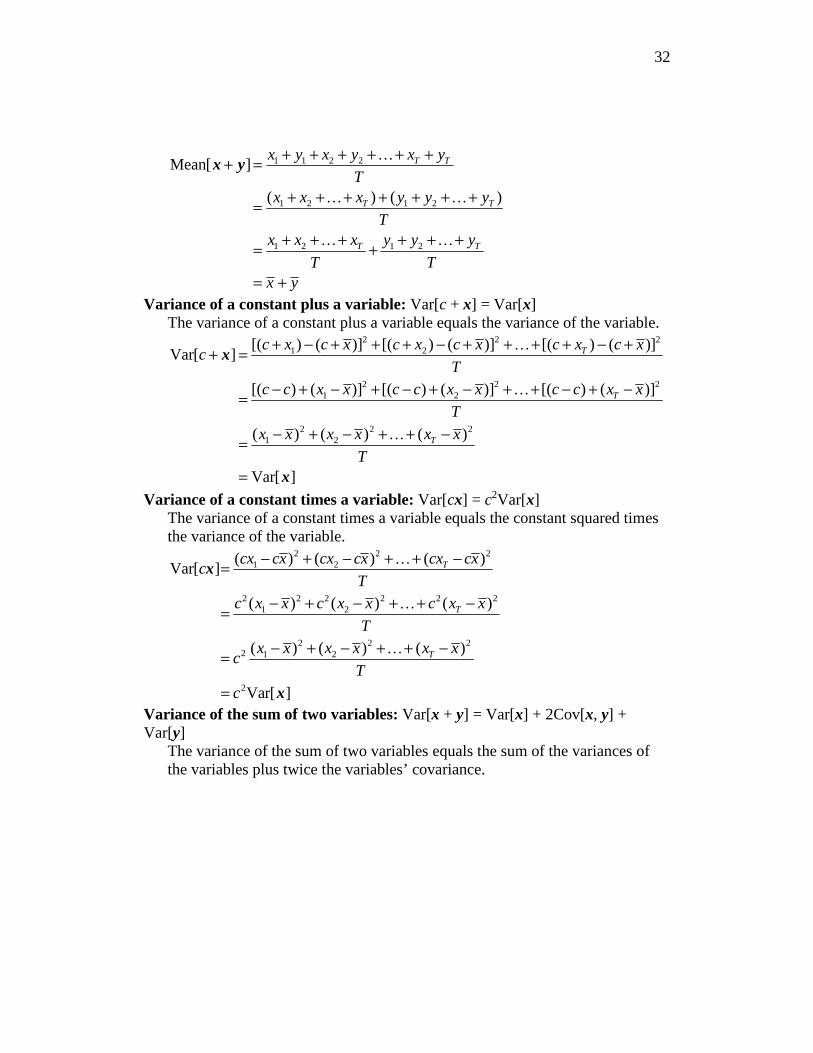
• Variance of a constant plus a variable: Var[c + x] = Var[x] The variance of a constant plus a variable equals the variance of the variable.

• Variance of a constant times a variable: Var[cx] = c2Var[x] The variance of a constant times a variable equals the constant squared times the variance of the variable.

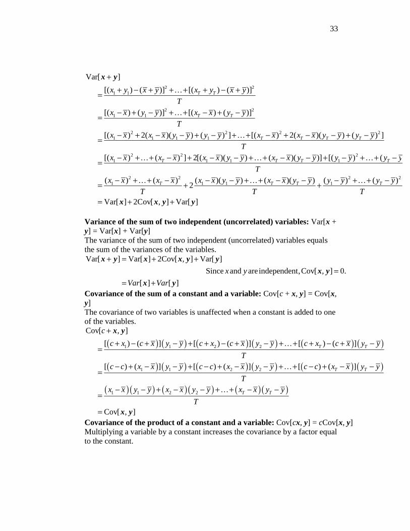
• Variance of the sum of two variables: Var[x + y] = Var[x] + 2Cov[x, y] + Var[y]

The variance of the sum of two variables equals the sum of the variances of the variables plus twice the variables’ covariance.

• Variance of the sum of two independent (uncorrelated) variables: Var[x + y] = Var[x] + Var[y]

The variance of the sum of two independent (uncorrelated) variables equals the sum of the variances of the variables.

• Covariance of the sum of a constant and a variable: Cov[c + x, y] = Cov[x, y]

The covariance of two variables is unaffected when a constant is added to one of the variables.

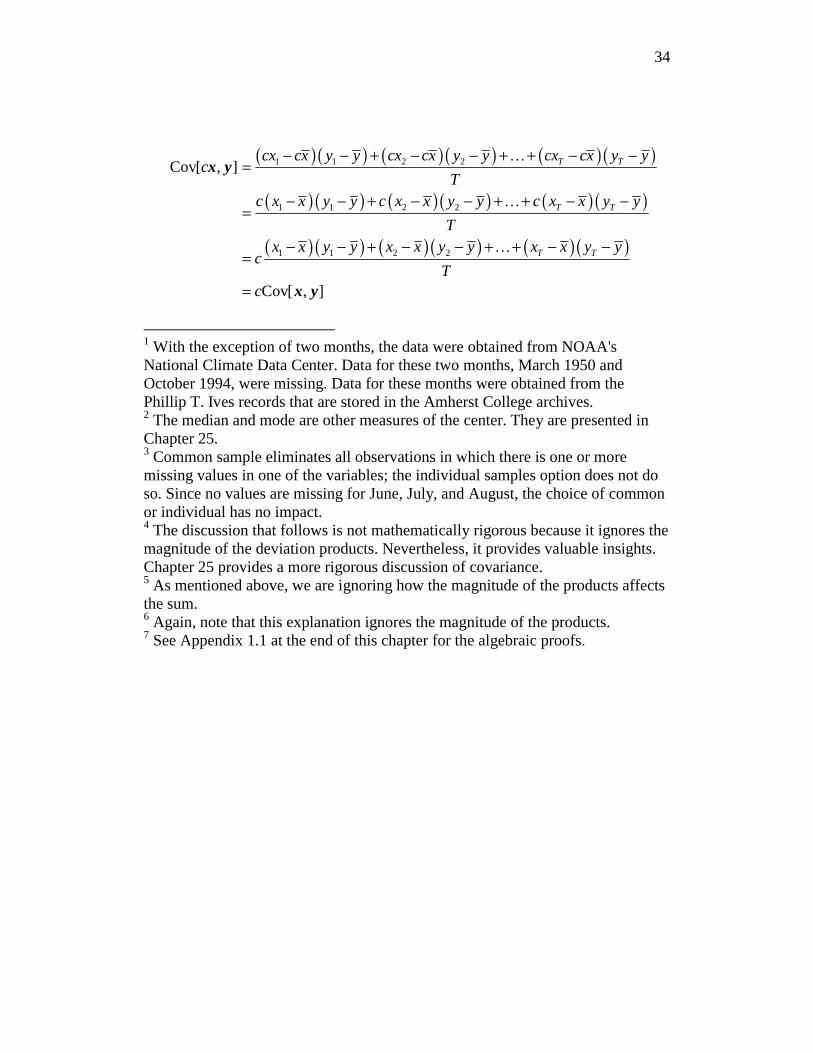
• Covariance of the product of a constant and a variable: Cov[cx, y] = cCov[x, y]

Multiplying one of the variables by a constant increases their covariance by a factor equal to the constant.

31

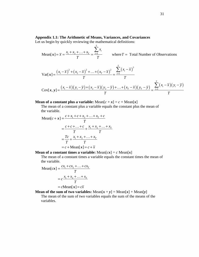
Appendix 1.1: The Arithmetic of Means, Variances, and Covariances Let us begin by quickly reviewing the mathematical definitions:

11 2Mean[ ] where Total Number of Observations

T

ttT

xx x x

x TT T

=+ + += = = =∑

x…

( ) ( ) ( ) ( )22 2 2

1 2 1Var[ ]

T

tT t

x xx x x x x x

T T=

−− + − + + −= =

∑x

…

( ) ( ) ( )( ) ( )( ) ( )( )1 1 2 2 1Cov[ , ]

T

t tT T t

x x y yx x y y x x y y x x y y

T T=

− −− − + − − + + − −= =

∑x y

…

Mean of a constant plus a variable: Mean[c + x] = c + Mean[x]

The mean of a constant plus a variable equals the constant plus the mean of the variable.

1 2

1 2

1 2

Mean[ ]

Mean[ ]

T

T

T

c x c x x cc

Tx x xc c c

T Tx x xTc

T Tc c x

+ + + + + ++ =

+ + ++ + += +

+ + += +

= + = +

x

x

…

……

…

Mean of a constant times a variable: Mean[cx] = c Mean[x] The mean of a constant times a variable equals the constant times the mean of the variable.

1 2

1 2

Mean[ ]

Mean[ ]

T

T

cx cx cxc

Tx x x

cT

c cx

+ + +=

+ + +=

= =

x

x

…

…

Mean of the sum of two variables: Mean[x + y] = Mean[x] + Mean[y] The mean of the sum of two variables equals the sum of the means of the variables.

32

1 1 2 2

1 2 1 2

1 2 1 2

Mean[ ]

( ) ( )

T T

T T

T T

x y x y x y

Tx x x y y y

Tx x x y y y

T Tx y

+ + + + + ++ =

+ + + + + + +=

+ + + + + += +

= +

x y…

… …

… …

Variance of a constant plus a variable: Var[c + x] = Var[x] The variance of a constant plus a variable equals the variance of the variable.

2 2 21 2

2 2 21 2

2 2 21 2

[( ) ( )] [( ) ( )] [( ) ( )]Var[ ]

[( ) ( )] [( ) ( )] [( ) ( )]

( ) ( ) ( )

Var[ ]

T

T

T

c x c x c x c x c x c xc

T

c c x x c c x x c c x x

T

x x x x x x

T

+ − + + + − + + + + − ++ =

− + − + − + − + + − + −=

− + − + + −=

=

x

x

…

…

…

Variance of a constant times a variable: Var[cx] = c2Var[x] The variance of a constant times a variable equals the constant squared times the variance of the variable.

2 2 21 2

2 2 2 2 2 21 2

2 2 22 1 2

2

( ) ( ) ( )Var[ ]

( ) ( ) ( )

( ) ( ) ( )

Var[ ]

T

T

T

cx cx cx cx cx cxc

T

c x x c x x c x x

T

x x x x x xc

T

c

− + − + + −=

− + − + + −=

− + − + + −=

=

x

x

…

…

…

Variance of the sum of two variables: Var[x + y] = Var[x] + 2Cov[x, y] + Var[y]

The variance of the sum of two variables equals the sum of the variances of the variables plus twice the variables’ covariance.

33

2 21 1

2 21 1

2 2 2 21 1 1 1

2 21 1 1

Var[ ]

[( ) ( )] [( ) ( )]

[( ) ( )] [( ) ( )]

[( ) 2( )( ) ( ) ] [( ) 2( )( ) ( ) ]

[( ) ( ) ] 2[( )( ) ( )( )]

T T

T T

T T T T

T T T

x y x y x y x y

T

x x y y x x y y

T

x x x x y y y y x x x x y y y y

T

x x x x x x y y x x y y

++ − + + + + − +=

− + − + + − + −=

− + − − + − + + − + − − + −=

− + + − + − − + + − −=

x y

…

…

…

… … 21

2 2 2 21 1 1 1

[( ) (

( ) ( ) ( )( ) ( )( ) ( ) ( )2

Var[ ] 2Cov[ , ] Var[ ]

T

T T T T

y y y y

T

x x x x x x y y x x y y y y y y

T T T

+ − + + −

− + + − − − + + − − − + + −= + +

= + +x x y y

…

… … …

Variance of the sum of two independent (uncorrelated) variables: Var[x + y] = Var[x] + Var[y] The variance of the sum of two independent (uncorrelated) variables equals the sum of the variances of the variables. Var[ ] Var[ ] 2Cov[ , ] Var[ ]

Since and are independent,Cov[ , ] 0.

[ ] [ ]

x y

Var Var

+ = + +=

= +

x y x x y y

x y

x yCovariance of the sum of a constant and a variable: Cov[c + x, y] = Cov[x, y] The covariance of two variables is unaffected when a constant is added to one of the variables.

( ) ( ) ( ) ( ) ( ) ( )

( ) ( ) ( ) ( ) ( ) ( )

( )( ) ( )( ) ( )( )

1 1 2 2

1 1 2 2

1 1 2 2

Cov[ , ]

[ ) ( ] [ ) ( ] [ ) ( ]

[ ) ( ] [ ) ( ] [ ) ( ]

Cov[ , ]

T T

T T

T T

c

c x c x y y c x c x y y c x c x y y

Tc c x x y y c c x x y y c c x x y y

Tx x y y x x y y x x y y

T

++ − + − + + − + − + + + − + −

=

− + − − + − + − − + + − + − −=

− − + − − + + − −=

=

x y

x y

…

…

…

Covariance of the product of a constant and a variable: Cov[cx, y] = cCov[x, y] Multiplying a variable by a constant increases the covariance by a factor equal to the constant.

34

( )( ) ( )( ) ( )( )

( ) ( ) ( )( ) ( ) ( )

( ) ( ) ( )( ) ( )( )

1 1 2 2

1 1 2 2

1 1 2 2

Cov[ , ]

Cov[ , ]

T T

T T

T T

cx cx y y cx cx y y cx cx y yc

Tc x x y y c x x y y c x x y y

Tx x y y x x y y x x y y

cT

c

− − + − − + + − −=

− − + − − + + − −=

− − + − − + + − −=

=

x y

x y

…

…

…

1 With the exception of two months, the data were obtained from NOAA's National Climate Data Center. Data for these two months, March 1950 and October 1994, were missing. Data for these months were obtained from the Phillip T. Ives records that are stored in the Amherst College archives. 2 The median and mode are other measures of the center. They are presented in Chapter 25. 3 Common sample eliminates all observations in which there is one or more missing values in one of the variables; the individual samples option does not do so. Since no values are missing for June, July, and August, the choice of common or individual has no impact. 4 The discussion that follows is not mathematically rigorous because it ignores the magnitude of the deviation products. Nevertheless, it provides valuable insights. Chapter 25 provides a more rigorous discussion of covariance. 5 As mentioned above, we are ignoring how the magnitude of the products affects the sum. 6 Again, note that this explanation ignores the magnitude of the products. 7 See Appendix 1.1 at the end of this chapter for the algebraic proofs.