Chapter 3: Interval Estimates and the Central Limit Theorem Chapter 3 Outline

• Review o Random Variables o Relative Frequency Interpretation of Probability

• Populations, Samples, Estimation Procedures, and the Estimate’s Probability Distribution

o Why Is the Mean of the Estimate’s Probability Distribution Important? Biased and Unbiased Estimation Procedures

o Why Is the Variance of the Estimate’s Probability Distribution Important? Reliability of Unbiased Estimation Procedures

• Interval Estimates • Central Limit Theorem • The Normal Distribution: A Way to Estimate Probabilities

o Properties of the Normal Distribution: o Using the Normal Distribution Table: An Example o Justifying the Use of the Normal Distribution o Normal Distribution’s Rules of Thumb

• Clint’s Dilemma and His Opinion Poll Chapter 3 Prep Questions 1. Consider a random process and the associated random variable.

a. What do we mean by a random variable? b. When dealing with a random variable:

1) What do we never know? 2) What can we hope to know?

2. Apply the arithmetic of means to show that

1 2

1Mean ( )[ ]T p

T+ + + =…v v v

whenever Mean[vt] = p for each t; that is, Mean[v1] = Mean[v2] = … = Mean[vT] = p.

2

3. Apply the arithmetic of variances to show that

1 2

1 (1 )Var ( )[ ]T

p p

T T

−+ + + =…v v v

whenever • Var[vt] = p(1−p) for each t; that is, Var[v1] = Var[v2] = … = Var[vT] =

p(1−p). and

• the vt’s are independent; that is, all the covariances equal 0. 4. What is the relative frequency interpretation of probability? 5. What two concepts have we introduced to describe a probability distribution? 6. Would you have more confidence in a poll that queries a small number of

individuals or a poll that queries a large number? Review

• Random Variables: Before the experiment is conducted: o Bad news. What we do not know: We cannot determine the

numerical value of the random variable with certainty. o Good news. What we do know: On the other hand, we can often

calculate the random variable’s probability distribution telling us how likely it is for the random variable to equal each of its possible numerical values.

• Relative Frequency Interpretation of Probability: After many, many repetitions of the experiment the distribution of the numerical values from the experiments mirrors the random variable’s probability distribution

Populations, Samples, Estimation Procedures, and the Estimate’s Probability Distribution Polling procedures use information gathered from a sample of the population to draw inferences about the entire population. In the previous chapter, we considered two unrealistic samples sizes, a sample size of 1 and a sample size of 2. Common sense suggests that such small samples would not be helpful in drawing inferences about an entire population. We considered these unrealistic sample sizes to lay the groundwork for realistic ones. We are now prepared to analyze the general case in which the sample size equals T. Let us return to our friend Clint who is running for president of his student body. Consider the following experiment:

3

Experiment 3.1: Opinion Poll with a Sample Size of T Write the names of every individual in the population on a card

• Perform the following procedure T times: o Thoroughly shuffle the cards. o Randomly draw one card. o Ask that individual if he/she supports Clint; the individual’s

answer determines the numerical value of vt: vt equals 1 if the tth individual polled supports Clint; 0 otherwise.

o Replace the card. • Calculate the fraction of those polled supporting Clint:

( )

1 2

1 2

where SampleSize

1=

T

T

v v vEstFrac T

T

v v vT

+ + += =

+ + +

…

…

The estimated fraction of the population supporting Clint, EstFrac, is a random variable. We cannot determine the numerical value of the estimated fraction, EstFrac, with certainty before the experiment is conducted. Question: What can we say about the random variable EstFrac? Answer: We can describe the center and spread of EstFrac’s probability distribution by calculating its mean and variance. Using the same logic as we applied in Chapter 2, we know the following:

• Mean[vt] = p for each t; that is, Mean[v1] = Mean[v2] = … = Mean[vT] = p.

• Var[vt] = p(1−p) for each t; that is, Var[v1] = Var[v2] = … = Var[vT] = p(1−p).

• the vt’s are independent; hence, their covariances equal 0. where p = ActFrac = Actual fraction of the population supporting Clint

4

Measure of the Probability Distribution Center: Mean of the Random Variable First, consider the mean. Apply the arithmetic of means and what we know about the vt’s:

( )1 2

1Mean[ ] Mean[ ]TT

= + + +…EstFrac v v v

Since Mean[cx] = cMean[x]

( )1 2

1= Mean[ ]TT

+ + +…v v v

Since Mean[x + y] = Mean[x] + Mean[y]

1 2

1= Mean[ ] Mean[ ] Mean[ ]( )TT

+ + +…v v v

Since Mean[v1] = Mean[v2] = … = Mean[vT] = p

1= ( )p p p

T+ + +…

How many p terms are there? A total of T. 1

= ( )T pT

×

Simplifying p=

Measure of the Probability Distribution Spread: Variance of the Random Variable Next, focus on the variance. Apply the arithmetic of variances and what we know about the vt’s:

( )1 2

1Var[ ] Var[ ]TT

= + + +…EstFrac v v v

Since Var[cx] = c2Var[x]

( )1 22

1= Var[ ]TT

+ + +…v v v

Since Var[x + y] = Var[x] + Var[y] when x and y are independent; hence, the covarainces are all 0.

1 22

1= [ ] Var[ ] Var[ ]( )TVar

T+ + +…v v v

Since Var[v1] = Var[v2] = … = Var[vT] = p(1 − p)

2

1= (1 ) (1 ) (1 )( )p p p p p p

T− + − + + −…

5

How many p(1 − p) terms are there? A total of T.

2

1= (1 )( )T p p

T× −

Simplifying. (1 )p p

T

−=

To summarize:

(1 )Mean[ ] Var[ ]

where Actual fraction of the population supporting Clint

Sample Size

p pp

Tp ActFrac

T

−= =

= ==

EstFrac EstFrac

Econometrics Lab 3.1: Polling – Checking the Mean and Variance Equations Once again we shall exploit the relative frequency interpretation of probability to check the equations for the mean and variance of the estimated fraction’s probability distribution:

Distribution of the Numerical Values

⏐ ⏐ ↓

After many, many

repetitions Probability Distribution

We just derived the mean and variance of the estimated fraction’s

probability distribution: (1 )

Mean[ ] Var[ ]

where

SampleSize

p pp

Tp ActFrac

T

−= =

==

EstFrac EstFrac

Consequently, after many, many repetitions, the mean of these numerical values should equal approximately p, the actual fraction of the population that supports

Clint, and the variance should equal approximately (1 )p p

T

−.

6

In the simulation, we begin by specifying the fraction of the population supporting Clint. We could choose any actual population fraction; for purposes of

illustration we choose 1

2 here.

1Actual fraction of the population supporting Clint .50

21 1 1 1 1

11 12 2 2 2 4Mean[ ] .50 Var[ ]2 4

( )

ActFrac

pT T T T

= = =

− ×= = = = = = =EstFrac EstFrac

We shall now use our simulation to consider different sample sizes, different T’s:

[Link to MIT Lab 3.1 goes here.]

Actual Population Fraction = ActFrac = p = .50

Equations: Simulation:

Sample Size

Mean of EstFrac’s

Probability Distribution

Variance of EstFrac’s

Probability Distribution

Simulation Repetitions

Mean (Average) of Numerical Values of EstFrac from the Experiments

Variance of Numerical Values of EstFrac from the Experiments

1 1

2= .50

1

4 = .25 >1,000,000 ≈.50 ≈.25

2 1

2= .50

1

8 = .125 >1,000,000 ≈.50 ≈.125

25 1

2= .50

1

100 = .01 >1,000,000 ≈.50 ≈.01

100 1

2= .50

1

400 = .0025 >1,000,000 ≈.50 ≈.0025

400 1

2= .50

1

1,600 = .000625 >1,000,000 ≈.50 ≈.000625

Table 3.1: Opinion Poll Simulation Results with Selected Sample Sizes

Our simulation results are consistent with the equations we derived. After many, many repetitions, the means of the numerical values equal the means of the estimated fraction’s probability distribution. The same is true for the variances.

7

Public opinion polls use procedures very similar to that described in our experiment. A specific number of people are asked who or what they support and then the results are reported. We can think of a poll as one repetition of our experiment. Pollsters use the numerical value of the estimated fraction from one repetition of the experiment to estimate the actual fraction. But how reliable is such an estimate? We shall now show that the reliability of an estimate depends on the mean and variance of the estimate’s probability distribution. Why Is the Mean of the Estimate’s Probability Distribution Important? Biased and Unbiased Estimation Procedures Recall Clint’s poll in which 12 of the 16 individuals queried supported him. The estimated fraction, EstFrac, equaled .75:

12.75

16EstFrac = =

In Chapter 2, we used our Opinion Poll simulation to show that this poll result did not prove with certainty that the actual fraction of the population supporting Clint exceeded .50. More generally, we observed that while it is possible for the estimated fraction to equal the actual population fraction, it is more likely for the estimated fraction to be greater than or less than the actual fraction. In other words, we cannot expect the estimated fraction from a single poll to equal the actual population fraction.

What, then, can we conclude? We know that the estimated fraction is a

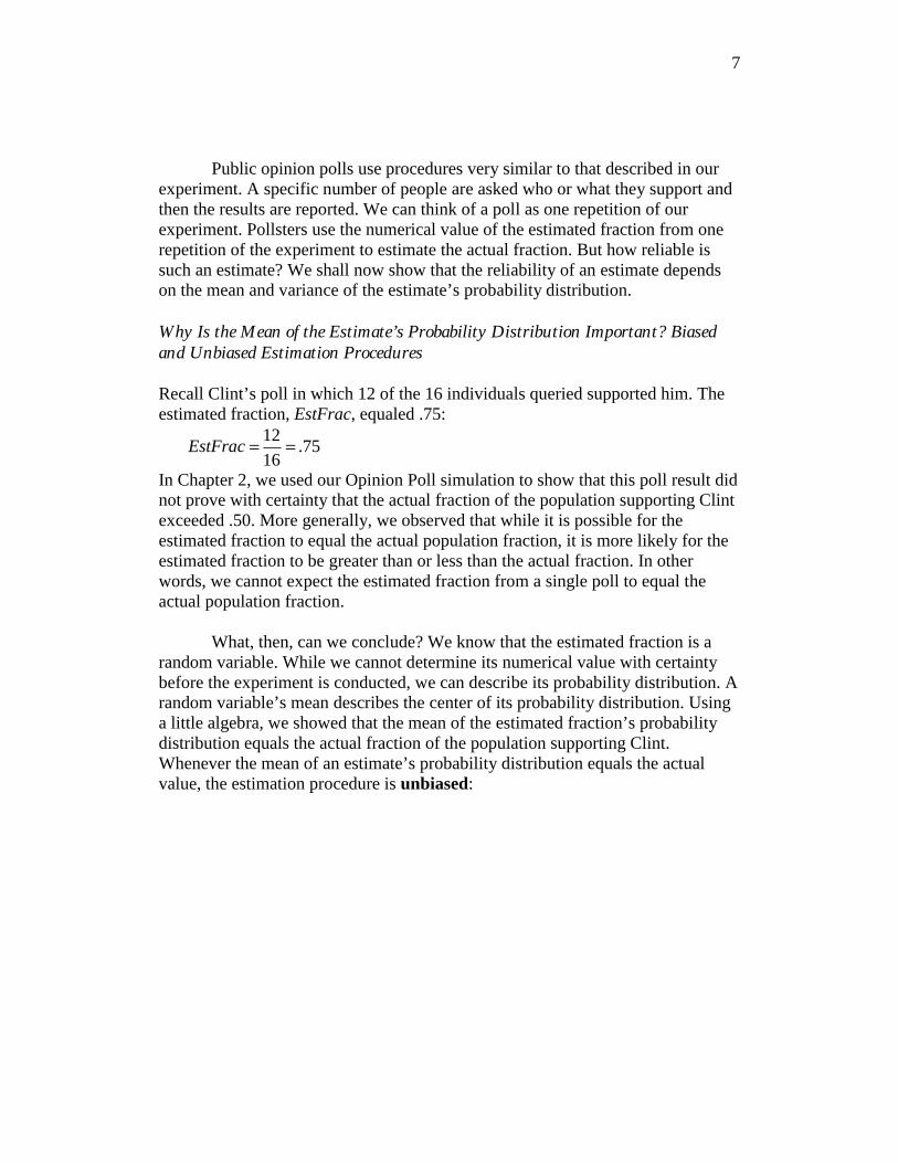
random variable. While we cannot determine its numerical value with certainty before the experiment is conducted, we can describe its probability distribution. A random variable’s mean describes the center of its probability distribution. Using a little algebra, we showed that the mean of the estimated fraction’s probability distribution equals the actual fraction of the population supporting Clint. Whenever the mean of an estimate’s probability distribution equals the actual value, the estimation procedure is unbiased:

8

Mean[EstFrac] = ActFrac

Probability Distribution

EstFrac

Figure 3.1: Probability Distribution of EstFrac Values

Unbiased Estimation Procedure ↓

Mean[EstFrac] = Actual Population Fraction = ActFrac Being unbiased is a very desirable property. An unbiased procedure does not systematically underestimate or overestimate the actual fraction of the population supporting Clint.

By exploiting the relative frequency interpretation of probability we can

use the simulations we just completed to confirm that Clint’s estimation procedure is unbiased.

Relative Frequency Interpretation of Probability: After many, many repetitions, the distribution of the numerical values mirrors the probability distribution.

⏐ ⏐ ↓

Unbiased Estimation Procedure

Average of the estimate’s ↓ numerical values after = Mean[EstFrac] = ActFrac

many, many repetitions é ã

Average of the estimate’s

= ActFrac numerical values after many, many repetitions

9

When the estimation procedure is unbiased, the average of the numerical values of the estimated fractions equaled the actual population fraction after many, many repetitions. Table 3.1 reports that this is true.

We can obtain even more intuition about unbiased estimation procedures

when the probability distribution of the estimate is symmetric. In this case, the chances that the estimated fraction will be less than the actual population fraction in one repetition equal the chances that the estimated fraction will be greater than the actual fraction. We shall use a simulation to illustrate this. Econometrics Lab 3.2: Polling – Illustrating the Importance of the Mean

[Link to MIT Lab 3.2 goes here.]

Figure 3.2: Opinion Poll Simulation

By default, an actual population fraction of .50 and a sample size of 100 are specified. Two new lists appear in the lower left of the window: a From list and a

10

To list. By default, a From value of .000 and a To value of .500 are selected. The From-To Percent line reports the percent of repetitions in which the estimated fraction lies between the From value, .000, and the To value, .500.

Check to be certain that the simulation is calculating the From-To Percent

correctly by clicking Start and then Continue a few times. Then, clear the Pause box and click Continue. After many, many repetitions, click Stop. The From-To Percent equals approximately 50 percent. The estimates in approximately 50 percent of the repetitions are less than .5, the actual value; consequently, approximately 50 percent of the repetitions are greater than .5, the actual value. The chances that the estimated fraction will be less than the actual population fraction in one repetition equal the chances that the estimated fraction will be greater than the actual fraction.

To summarize, there are two important points to make about Clint’s poll:

• Bad news: We cannot expect the estimated fraction from Clint’s poll, .75, to equal the actual population fraction.

• Good news: The estimation procedure that Clint used is unbiased. The mean of the estimated fraction’s probability distribution equals the actual population fraction:

Mean[EstFrac] = Actual Population Fraction = ActFrac The estimation procedure does not systematically underestimate or overestimate the actual population fraction. If the probability distribution is symmetric, the chances that the estimated fraction will be less than the actual population fraction equal the chances that the estimated fraction will be greater.

Why Is the Variance of the Estimate’s Probability Distribution Important? Reliability of Unbiased Estimation Procedures We shall use the Polling Simulation to illustrate the importance of the probability distribution’s variance. Econometrics Lab 3.3: Polling – Illustrating the Importance of the Variance In addition to specifying the actual population fraction and the sample size, the simulation includes the From-To lists.

[Link to MIT Lab 3.3 goes here.]

11

As before, the actual population fraction equals .50 by default. Select .450 from the “From” list and .550 from the “To” list. The simulation will now calculate the percent of the repetitions in which the numerical value of the estimated fraction lies within the .450-.550 interval. Since we have specified the actual population fraction to be .50, the simulation will report the percent of repetitions in which the numerical value of the estimate fraction lies within .05 of the actual fraction. Initially, a sample size of 25 is selected. Note that the Pause checkbox is cleared. Click Start and then after many, many repetitions, click Stop. Next, consider sample sizes of 100 and 400. Table 3.2 reports the results for the three sample sizes:

Actual Population Fraction = ActFrac = p = .50 ⇒ Mean[EstFrac] = .50 Variance of Simulation: Percent of Repetitions

Sample EstFrac’s Probability Simulation in which the Numerical Value of Size Distribution Repetitions EstFrac Lies between .45 and .55 25 .01 >1,000,000 ≈39%

100 .0025 >1,000,000 ≈69% 400 .000625 >1,000,000 ≈95%

Table 3.2: Opinion Poll From-To Simulation Results When the sample size is 25, the numerical value of the estimated fraction

falls within .05 of the actual population fraction in about 39 percent of the repetitions. When the sample size is 100, the numerical value of the estimated fraction falls within .05 of the actual population fraction in about 69 percent of the repetitions. When the sample size is 400, the numerical value of the estimated fraction falls within .05 of the actual population fraction in about 95 percent of the repetitions.

Sample size = 25 Sample size = 100 Sample size = 400

.50 .50 .50.45 .55 .45 .55 .45 .55

39% 69%95%

Figure 3.3: Histograms of Estimated Fraction Numerical Values

The variance plays the key role here. When the variance is large, the

distribution is “spread out”; the numerical value of the estimated fraction falls

12

within .05 of the actual fraction relatively infrequently. On the other hand, when the variance is small, the distribution is tightly “cropped” around the actual population fraction, .50; consequently, the numerical value of the estimated fraction falls within .05 of the actual population fraction more frequently.

13

Interval Estimates We can now exploit the relative frequency interpretation of probability to obtain a quantitative sense of how much confidence we should have in the results of a single opinion poll. We do so by considering the following interval estimate question:

Interval Estimate Question: What is the probability that the numerical value of the estimated fraction, EstFrac, from one repetition of the experiment lies within ___ of the actual population fraction, ActFrac? ______

Since we are focusing on the interval from .450 to .550 and the actual population fraction is specified as .50, we can enter .05 in the first blank:

Interval Estimate Question: What is the probability that the numerical value of the estimated fraction, EstFrac, from one repetition of the experiment lies within .05 of the actual population fraction, ActFrac? ______

Begin by focusing on a sample size of 25. In view of what we just learned

from the simulation, we can now answer the interval estimate question. After many, many repetitions of the experiment, the numerical value of the estimated fraction falls within .05 of the actual value about 39 percent of the time. Now, apply the relative frequency interpretation of probability:

Relative Frequency Interpretation of Probability: When the experiment is repeated many, many times, the relative frequency of each outcome equals its probability.

Consequently, the probability that the numerical value of the estimated

fraction in one repetition of the experiment falls within .05 of the actual value is about .39. Using the same logic, when the sample size is 100 the probability that the numerical value of the estimated fraction in one repetition of the experiment will fall within .05 of the actual value is about .69. When the sample size is 400 the probability that the numerical value of the estimated fraction in one repetition of the experiment will fall within .05 of the actual value is about .95.

Actual Population Fraction = ActFrac = p = .50 ⇒ Mean[EstFrac] = .50

Variance After many, many repetitions, In a single poll, of EstFrac’s the percent of repetitions in the probability that

Sample probability which EstFrac falls within the EstFrac falls within the Size distribution interval from .45 to .55 interval from .45 to .55 25 .01 ≈39% ≈.39

100 .0025 ≈69% ≈.69 400 .000625 ≈95% ≈.95

Table 3.3: Interval Estimate Question and Opinion Poll Simulation Results

14

Sample size = 25 Sample size = 100 Sample size = 400

.50 .50 .50.45 .55 .45 .55 .45 .55

.39.95

.69

Figure 3.4: Probability Distribution of Estimated Fraction Values

As the sample size becomes larger, it becomes more likely that the estimated fraction resulting from a single poll will be close to the actual population fraction. This is consistent with our intuition, is it not? When more people are polled we have more confidence that the estimated fraction will be close to the actual value.

We can now generalize what we just learned. When an estimation

procedure is unbiased, the variance of the estimate’s probability distribution is important because it determines the likelihood that the estimate will be close to the actual value.

Figure 3.5: Probability Distribution of Estimated Fraction Values

15

When the probability distribution’s variance is large, it is unlikely that the estimated fraction from one poll will be close to the actual population fraction; consequently, the estimated fraction is an unreliable estimate of the actual population fraction. On the other hand, when the probability distribution’s variance is small, it is likely that the estimated fraction from one poll will be close to the actual population fraction; in this case, the estimated fraction is a reliable estimate of the actual population fraction. Central Limit Theorem You may have noticed that the distributions of the numerical values produced by the simulation for the samples of 25, 100, and 400 look like bell shaped curves. Although we shall not provide a proof, it can be shown that as the sample size increases, the distribution gradually approaches what mathematicians and statisticians call the normal distribution. Formally, this result is known as the Central Limit Theorem. Econometrics Lab 3.4: The Central Limit Theorem We shall illustrate the Central Limit Theorem by using our Opinion Poll Simulation. Again, let the actual population fraction equal .50 and consider three different sample sizes: 25, 100, and 400. In each case, we shall use our simulation to calculate interval estimates for 1, 2, and 3 standard deviations around the mean.

[Link to MIT Lab 3.4 goes here.]

First, consider a sample size of 25:

1Sample Size 25 Actual Population Fraction .50

21 1 1

1 (1 ) 12 2 4Mean[ ] .50 Var[ ]2 25 25 100

1 1SD[ ] Var[ ] .10

100 10

T ActFrac

p pp

T

= = = = =

×−= = = = = = =

= = = =

EstFrac EstFrac

EstFrac EstFrac

16

When the sample size equals 25, the standard deviation is .10. Since the distribution mean equals the actual population fraction, .50, 1 standard deviation around the mean would be from .400 to .600, 2 standard deviations from .300 to .700, and 3 standard deviations from .200 to .800. In each case, specify the appropriate From and To values and be certain that the Pause checkbox is cleared. Click Start and then after many, many repetitions click Stop. The simulation results are reported in Table 3.4:

Interval: Simulation: Standard Deviations within Percent of repetitions Random Variable’s Mean From To within interval

1 .400 .600 69.25% 2 .300 .700 96.26% 3 .200 .800 99.85%

Table 3.4: Interval Percentages for a Sample Size of 25

Next, a sample size of 100: 1

Sample Size 100 Actual Population Fraction .502

1 1 11 (1 ) 12 2 4Mean[ ] .50 Var[ ]2 100 100 400

1 1SD[ ] Var[ ] .05

400 20

T ActFrac

p pp

T

= = = = =

×−= = = = = = =

= = = =

EstFrac EstFrac

EstFrac EstFrac

When the sample size equals 100, the standard deviation is .05. Since the distribution mean equals the actual population fraction, .50, 1 standard deviation around the mean would be from .450 to .550, 2 standard deviations from .400 to .600, and 3 standard deviations from .350 to .650.

Interval: Simulation: Standard Deviations within Percent of repetitions Random Variable’s Mean From To within interval

1 .450 .550 68.50% 2 .400 .600 95.64% 3 .350 .650 99.77%

Table 3.5: Interval Percentages for a Sample Size of 100

17

Last, consider a sample size of 400: 1

Sample Size 400 Actual Population Fraction .502

1 1 11 (1 ) 12 2 4Mean[ ] .50 Var[ ]2 400 400 1,600

1 1SD[ ] Var[ ] .025

1,600 40

T ActFrac

p pp

T

= = = = =

×−= = = = = = =

= = = =

EstFrac EstFrac

EstFrac EstFrac

When the sample size equals 400, the standard deviation is .025. Since the distribution mean equals the actual population fraction, .5, 1 standard deviation around the mean would be from .475 to .525; 2 standard deviations from .450 to .550, and 3 standard deviations from .425 to .575.

Interval: Simulation: Standard Deviations within Percent of repetitions

Distribution Mean From To within interval 1 .475 .525 68.29% 2 .450 .550 95.49% 3 .425 .575 99.73%

Table 3.6: Interval Percentages for a Sample Size of 400

Let us summarize the simulation results in a single table:

Sample Sizes Mean[EstFrac] 25 100 400 SD[EstFrac] .100 .050 .025

Interval: 1 SD

From-To Values .400-.600 .450-.550 .475-.525 Percent of Repetitions 69.25% 68.50% 68.29%

Interval: 2 SD

From-To Values .300 .700 .400-.600 .450-.550 Percent of Repetitions 96.26% 95.64% 95.49%

Interval: 3 SD

From-To Values 200-.800 .350-.650 .425-.575 Percent of Repetitions 99.85% 99.77% 99.73%

Table 3.7: Summary of Interval Percentages Results

18

Clearly, standard deviations play a crucial and consistent role here. Regardless of the sample size, approximately 68 or 69 percent of the repetitions fall within one standard deviation of the mean, approximately 95 or 96 percent within two standard deviations, and more than 99 percent within three. The normal distribution exploits the key role played by standard deviations. The Normal Distribution: A Way to Calculate Interval Estimates The normal distribution is a symmetric, bell-shaped curve with the midpoint of the bell occurring at the distribution mean. The total area lying beneath the curve is 1.0. As mentioned before, it can be proven rigorously that as the sample size increases, the probability distribution of the estimated fraction approaches the normal distribution. This fact allows us to use the normal distribution to estimate probabilities for interval estimates.

Distribution

Probability Distribution

Mean

v

Figure 3.6: Normal Distribution

Nearly every econometrics and statistics textbook includes a table that

describes the normal distribution. We shall now learn how to use the table to estimate the probability that a random variable will lie between any two values. The table is based on the “normalized value” of the random variable. By convention, the normalized value is denoted by the letter z:

Valueof Random Variable Mean of Random Variable's Probability Distribution

Standard Deviation of Random Variable's Probability Distributionz

−=

19

Let us express this a little more concisely: Valueof Random Variable Distribution Mean

DistributionStandard Deviationz

−=

DistributionMean

SD’s

Probability of beingmore than z standarddeviations above the

distribution mean

Probability Distribution

z

Right Tail Probability

v

Figure 3.7: Normal Distribution Right Tail Probabilities

In words, z tells us by how many standard deviations the value lies from the mean. If the value of the random variable equals the mean, z equals .0; if the value is one standard deviation above the mean, z equals 1.0; if the value is two standard deviations above the mean, z equals 2.0; etc.

The equation that describes the normal distribution is complicated (see

Appendix 3.1). Fortunately, we can avoid using the equation because tables are available that describe the distribution. The entire table appears in Appendix 3.1; an abbreviated portion appears below in Table 3.8:

z 0.00 0.01 0.02 0.03 0.04 0.05 0.06 0.07 0.08 0.09 . . .

0.4 0.3446 0.3409 0.3372 0.3336 0.3300 0.3264 0.3228 0.3192 0.3156 0.3121 0.5 0.3085 0.3050 0.3015 0.2981 0.2946 0.2912 0.2877 0.2843 0.2810 0.2776 0.6 0.2743 0.2709 0.2676 0.2643 0.2611 0.2578 0.2546 0.2514 0.2483 0.2451 . . . 1.4 0.0808 0.0793 0.0778 0.0764 0.0749 0.0735 0.0721 0.0708 0.0694 0.0681 1.5 0.0668 0.0655 0.0643 0.0630 0.0618 0.0606 0.0594 0.0582 0.0571 0.0559 1.6 0.0548 0.0537 0.0526 0.0516 0.0505 0.0495 0.0485 0.0475 0.0465 0.0455 . . .

Table 3.8: Right Tail Probabilities for the Normal Distribution

20

The row of the normal distribution table specifies the z value’s whole number and its tenths; the column the z value’s hundredths. The numbers within the body of the table estimate the probability that the random variable lies more than z standard deviations above its mean. Properties of the Normal Distribution:

• The normal distribution is bell shaped. • The normal distribution is symmetric around its mean (center). • The area beneath the normal distribution equals 1.0.

Using the Normal Distribution Table: An Example For purposes of illustration, suppose that we want to use the normal distribution to calculate the probability that the estimated fraction from one repetition of the experiment would fall between .525 and .575 when the actual population fraction was .50 and the sample size was 100. We begin by calculating the probability distribution’s mean and standard deviation:

1Sample Size 100 Actual Population Fraction .50

21 1 1

1 (1 ) 12 2 4Mean[ ] .50 Var[ ]2 100 100 400

1 1SD[ ] Var[ ] .05

400 20

T ActFrac

p pp

T

= = = = =

×−= = = = = = =

= = = =

EstFrac EstFrac

EstFrac EstFrac

21

DistributionMean = .50

Probability Distribution

EstFrac.525 .575

Prob[EstFrac Between .525 and .575]

Figure 3.8: Interval Estimate from .525 to .575

To calculate the probability that the estimated fraction lies between .525

and .575, we first calculate the z-values for .525 and .575; that is, we calculate the number of standard deviations that .525 and .575 lie from the mean. Since the mean equals .500 and the standard deviation equals .05,

• z-value for .525 equals .50:

.525 .500 .025 1.50

.05 .05 2z

−= = = =

.525 lies a half standard deviation above the mean.

• z-value for .575 equals 1.50: .575 .500 .075 3

1.50.05 .05 2

z−= = = =

.575 lies one and a half standard deviations above the mean.

z 0.00 0.01 0.4 0.3446 0.3409 0.5 0.3085 0.3050 0.6 0.2743 0.2709

1.4 0.0808 0.0793 1.5 0.0668 0.0655

Table 3.9: Selected Right Tail Probabilities for the Normal Distribution

22

Next, consider the right tail probabilities for the normal distribution. When

we use this table we implicitly assume that the normal distribution accurately describes the estimated fraction’s probability distribution. For the moment, assume that this is true. The entry corresponding to z equaling .50 is .3085; this tells us that the probability that the estimated fraction lies above .525 is .3085.

Prob[EstFrac Greater Than .525] = .3085

.3085

Probability Distribution

.50 SD.50 .525

EstFrac

Figure 3.9a: Probability of EstFrac Greater than .525

23

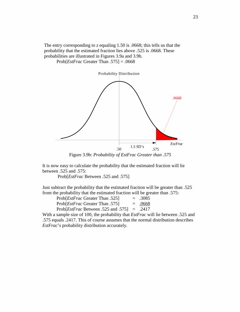
The entry corresponding to z equaling 1.50 is .0668; this tells us that the probability that the estimated fraction lies above .525 is .0668. These probabilities are illustrated in Figures 3.9a and 3.9b.

Prob[EstFrac Greater Than .575] = .0668

.50

.0668

Probability Distribution

1.5 SD’s.575

EstFrac

Figure 3.9b: Probability of EstFrac Greater than .575

It is now easy to calculate the probability that the estimated fraction will lie between .525 and .575:

Prob[EstFrac Between .525 and .575] Just subtract the probability that the estimated fraction will be greater than .525 from the probability that the estimated fraction will be greater than .575:

Prob[EstFrac Greater Than .525] = .3085 Prob[EstFrac Greater Than .575] = .0668 Prob[EstFrac Between .525 and .575] = .2417

With a sample size of 100, the probability that EstFrac will lie between .525 and .575 equals .2417. This of course assumes that the normal distribution describes EstFrac’s probability distribution accurately.

24

Justifying the Use of the Normal Distribution To justify using the normal distribution to calculate the probabilities, reconsider our simulations in which we calculated the percent of repetitions that fall within 1, 2, and 3 standard deviations of the mean after many, many repetitions. Now, use the normal distribution to calculate these percentages.

We can now calculate the probability of being within one, two, and three

standard deviations of the mean by reviewing two important properties of the normal distribution:

• The normal distribution is symmetric about its mean. • The area beneath the normal distribution equals 1.0.

We begin with the one standard deviation (SD) case. Table 3.10 reports that the right hand tail probability for z = 1.00 equals .1587:

Prob[1 SD Above] = .1587

z 0.00 0.01 z 0.00 0.01 z 0.00 0.01 0.9 0.1841 0.1814 1.9 0.0287 0.0281 2.9 0.0019 0.0018 1.0 0.1587 0.1562 2.0 0.0228 0.0222 3.0 0.0013 0.0013 1.1 0.1357 0.1335 2.1 0.0179 0.0174

Table 3.10: Right Tail Probabilities for the Normal Distribution We shall now use that to calculate the probability of being within 1 standard deviation of the mean:

• Since the normal distribution is symmetric, the probability of being more than one standard deviation above the mean equals the probability of being more than one standard deviation below the mean.

Prob[1 SD Below] = Prob[1 SD Above] = .1587

• Since the area beneath the normal distribution equals 1.0, the probability of being within one standard deviation of the mean equals 1.0 less the sum of the probabilities of being more than one standard deviation above the mean and the probalibity of being more than one standard deviation below the mean.

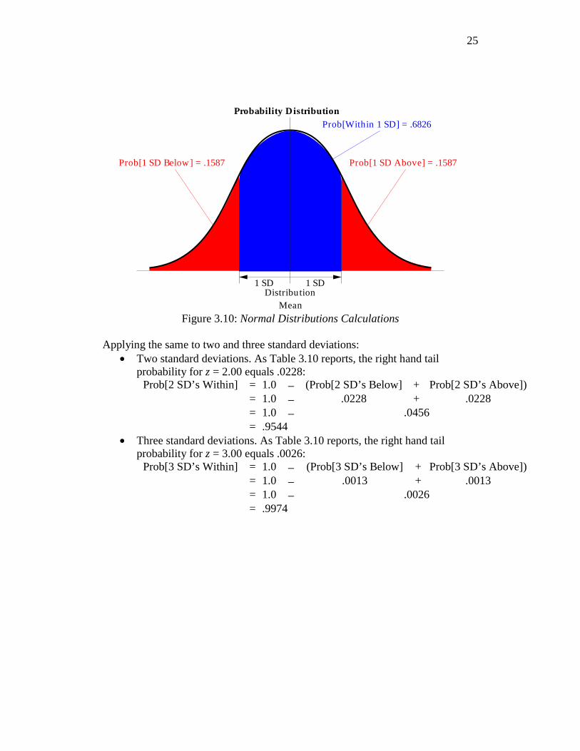
Prob[1 SD Within] = 1.0 − (Prob[1 SD Below] + Prob[1 SD Above]) = 1.0 − .1587 + .1587 = 1.0 − .3174 = .6826

25

DistributionMean

1 SD 1 SD

Probability Distribution

Prob[1 SD Above] = .1587Prob[1 SD Below] = .1587

Prob[Within 1 SD] = .6826

Figure 3.10: Normal Distributions Calculations

Applying the same to two and three standard deviations:

• Two standard deviations. As Table 3.10 reports, the right hand tail probability for z = 2.00 equals .0228:

Prob[2 SD’s Within] = 1.0 − (Prob[2 SD’s Below] + Prob[2 SD’s Above]) = 1.0 − .0228 + .0228 = 1.0 − .0456 = .9544

• Three standard deviations. As Table 3.10 reports, the right hand tail probability for z = 3.00 equals .0026:

Prob[3 SD’s Within] = 1.0 − (Prob[3 SD’s Below] + Prob[3 SD’s Above]) = 1.0 − .0013 + .0013 = 1.0 − .0026 = .9974

26

Table 3.11 compares the percentages calculated from our simulations with the percentages that would be predicted by the normal distribution.

Interval: Standard Deviations within

Distribution Mean

Simulation: Percent of Repetitions

Within Interval Sample Size

Normal Distribution Percentages 25 100 400

1 69.25% 68.50% 68.29% 68.26% 2 96.26% 95.64% 95.49% 95.44% 3 99.85% 99.77% 99.74% 99.74%

Table 3.11: Interval Percentages Results and Normal Distribution Percentages

Table 3.11 reveals that the normal distribution percentages are good approximations of the simulation percentages. Furthermore, as the sample size increases, the percent of repetitions within each interval gets closer and closer to the normal distribution percentages. This is precisely what the Central Limit Theorem concludes. We use the normal distribution to calculate interval estimates because it provides estimates that are close to the actual values. Normal Distribution’s Rules of Thumb Table 3.12 illustrates what are sometimes called the normal distribution’s “rules of thumb”:

Standard Deviations Probability from the Mean of being within

1 ≈.68 2 ≈.95 3 >.99

Table 3.12: Normal Distribution Rules of Thumb

In round numbers, the probability of being within 1 standard deviation of the mean is .68, the probability of being within 2 standard deviations is .95, and the probability of being within 3 standard deviations is more than .99.

27

Clint’s Dilemma and His Opinion Poll We shall now return to Clint’s dilemma. The election is tomorrow and Clint must decide whether or not to hold a pre-election beer tap rally designed to entice more students to vote for him. If Clint is comfortably ahead, he could save his money and not hold the beer tap rally. On the other hand, if the election is close, the beer tap rally could be critical. Ideally, Clint would like to contact each individual in the student body, but time does not permit this to happen.

In view of the lack of time, Clint decides to poll a sample of 16 students in

the population. Clint has adopted the philosophy of econometricians: Econometrician’s Philosophy: If you lack the information to determine the value directly, estimate the value to the best of your ability using the information you do have.

More specifically, he wrote the name of each student on a 3×5 card and repeated the following procedure 16 times:

• Thoroughly shuffle the cards. • Randomly draw one card. • Ask that individual if he/she supports Clint and record the answer. • Replace the card.

After conducting his poll, Clint learns that 12 of the 16 students polled support him. That is, the estimated fraction of the population supporting Clint is .75:

12 3Estimated Fraction of the Population Supporting Clint: .75

16 4EstFrac = = =

Based on the results of the poll, it looks like Clint is ahead. But how confident should he be that this is in fact true? We shall address this question in the next chapter.

28

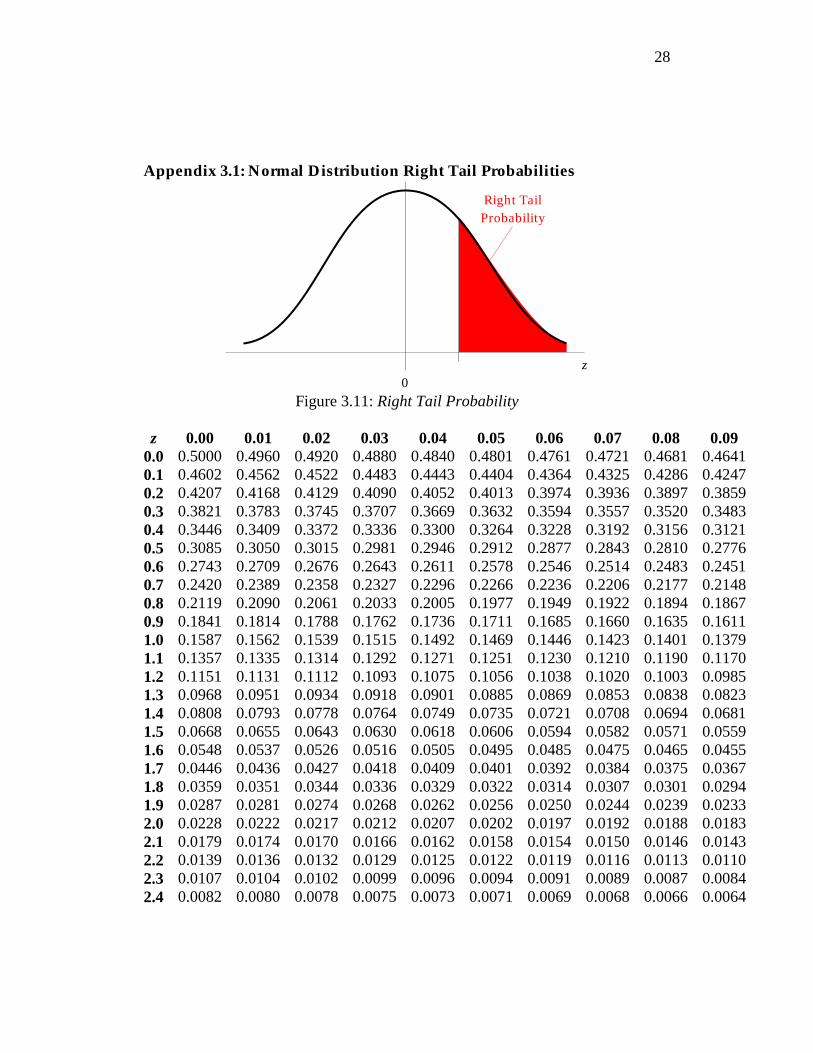
Appendix 3.1: Normal Distribution Right Tail Probabilities

0z

Right TailProbability

Figure 3.11: Right Tail Probability

z 0.00 0.01 0.02 0.03 0.04 0.05 0.06 0.07 0.08 0.09

0.0 0.5000 0.4960 0.4920 0.4880 0.4840 0.4801 0.4761 0.4721 0.4681 0.4641 0.1 0.4602 0.4562 0.4522 0.4483 0.4443 0.4404 0.4364 0.4325 0.4286 0.4247 0.2 0.4207 0.4168 0.4129 0.4090 0.4052 0.4013 0.3974 0.3936 0.3897 0.3859 0.3 0.3821 0.3783 0.3745 0.3707 0.3669 0.3632 0.3594 0.3557 0.3520 0.3483 0.4 0.3446 0.3409 0.3372 0.3336 0.3300 0.3264 0.3228 0.3192 0.3156 0.3121 0.5 0.3085 0.3050 0.3015 0.2981 0.2946 0.2912 0.2877 0.2843 0.2810 0.2776 0.6 0.2743 0.2709 0.2676 0.2643 0.2611 0.2578 0.2546 0.2514 0.2483 0.2451 0.7 0.2420 0.2389 0.2358 0.2327 0.2296 0.2266 0.2236 0.2206 0.2177 0.2148 0.8 0.2119 0.2090 0.2061 0.2033 0.2005 0.1977 0.1949 0.1922 0.1894 0.1867 0.9 0.1841 0.1814 0.1788 0.1762 0.1736 0.1711 0.1685 0.1660 0.1635 0.1611 1.0 0.1587 0.1562 0.1539 0.1515 0.1492 0.1469 0.1446 0.1423 0.1401 0.1379 1.1 0.1357 0.1335 0.1314 0.1292 0.1271 0.1251 0.1230 0.1210 0.1190 0.1170 1.2 0.1151 0.1131 0.1112 0.1093 0.1075 0.1056 0.1038 0.1020 0.1003 0.0985 1.3 0.0968 0.0951 0.0934 0.0918 0.0901 0.0885 0.0869 0.0853 0.0838 0.0823 1.4 0.0808 0.0793 0.0778 0.0764 0.0749 0.0735 0.0721 0.0708 0.0694 0.0681 1.5 0.0668 0.0655 0.0643 0.0630 0.0618 0.0606 0.0594 0.0582 0.0571 0.0559 1.6 0.0548 0.0537 0.0526 0.0516 0.0505 0.0495 0.0485 0.0475 0.0465 0.0455 1.7 0.0446 0.0436 0.0427 0.0418 0.0409 0.0401 0.0392 0.0384 0.0375 0.0367 1.8 0.0359 0.0351 0.0344 0.0336 0.0329 0.0322 0.0314 0.0307 0.0301 0.0294 1.9 0.0287 0.0281 0.0274 0.0268 0.0262 0.0256 0.0250 0.0244 0.0239 0.0233 2.0 0.0228 0.0222 0.0217 0.0212 0.0207 0.0202 0.0197 0.0192 0.0188 0.0183 2.1 0.0179 0.0174 0.0170 0.0166 0.0162 0.0158 0.0154 0.0150 0.0146 0.0143 2.2 0.0139 0.0136 0.0132 0.0129 0.0125 0.0122 0.0119 0.0116 0.0113 0.0110 2.3 0.0107 0.0104 0.0102 0.0099 0.0096 0.0094 0.0091 0.0089 0.0087 0.0084 2.4 0.0082 0.0080 0.0078 0.0075 0.0073 0.0071 0.0069 0.0068 0.0066 0.0064

29

2.5 0.0062 0.0060 0.0059 0.0057 0.0055 0.0054 0.0052 0.0051 0.0049 0.0048 2.6 0.0047 0.0045 0.0044 0.0043 0.0041 0.0040 0.0039 0.0038 0.0037 0.0036 2.7 0.0035 0.0034 0.0033 0.0032 0.0031 0.0030 0.0029 0.0028 0.0027 0.0026 2.8 0.0026 0.0025 0.0024 0.0023 0.0023 0.0022 0.0021 0.0021 0.0020 0.0019 2.9 0.0019 0.0018 0.0018 0.0017 0.0016 0.0016 0.0015 0.0015 0.0014 0.0014 3.0 0.0013 0.0013 0.0013 0.0012 0.0012 0.0011 0.0011 0.0011 0.0010 0.0010

Valueof Random Variable Distribution Mean Mean[ ]

DistributionStandard Deviation SD[ ]

xz

− −= = xx

1 [ ]

2 [ ]1Normal Distribution Probability Density Function:

SD[ ] 2

( )x Mean

SDeπ

−− xx

x