Embed Size (px)
Citation preview
Chapter 1
International Financial Markets:
Basic Concepts
In daily life, we find ourselves in constant contact with internationally traded goods. If you
enjoy music, you may play a U.S. manufactured CD of music by a Polish composer through
a Japanese amplifier and British speakers. You may be wearing clothing made in China or
eating fruit from Chile. As you drive to work, you will see cars manufactured in half a dozen
different countries on the streets.
Less visible in daily life is the international trade in financial assets, but its dollar volume
is much greater. This trade takes place in the international financial markets. When inter-
national trade in financial assets is easy and reliable—due to low transactions costs in liquid
markets—we say international financial markets are characterized by high capital mobility.
Financial capital was highly mobile in the nineteenth century. The early twentieth cen-
tury brought two world wars and the Great Depression. Many governments implemented
controls on international capital flows, which fragmented the international financial markets
and reduced capital mobility. Postwar efforts to increase the stability and integration of
markets for goods and services included the creation of the General Agreement on Tariffs
and Trade (the GATT, the precursor to the World Trade Organization, or WTO). Until
1
2 CHAPTER 1. FINANCIAL MARKETS
recently, no equivalent efforts addressed international trade in securities. The low level of
capital mobility is reflected in the economic models of the 1950s and 1960s: economists felt
comfortable conducting international analyses under the assumption of capital immobility.
Financial innovations, such as the Eurocurrency markets, undermined the effectiveness of
capital controls.1 Technological innovations lowered the costs of international transactions.
These factors, combined with the liberalizations of capital controls in the 1970s and 1980s, led
to the development of highly integrated world financial markets. Economists have responded
to this “globalization” of financial markets, and they now usually adopt perfect capital
mobility as a reasonable approximation of conditions in the international financial markets.
International capital flows surged after the oil shock of 1973–74, which spurred financial
intermediation on a global scale. Surpluses in the oil-exporting countries and corresponding
deficits among oil importers led to a recycling of “petrodollars” in the growing Euromar-
kets. Many developing countries gained new access to international capital markets, where
they financed mounting external imbalances. Most of this intermediation occurred in the
form of bank lending, and large banks in the industrial countries accepted huge exposures
to developing country debt. The debt crisis of the 1980s led to a significant slowdown in
capital flows to emerging markets.2 The waning of the debt crisis led to new large-scale
private capital inflows to emerging markets in the 1990s.3 Private capital responded to the
efforts of many Latin American countries to liberalize, privatize, open markets, and enhance
macroeconomic stability. Countries in Central and Eastern Europe began a transition to-
ward market economies, and rapid growth in a group of economies in East Asia had caught
the attention of investors worldwide. Net long-term private flows to developing countries
increased from $42 billion in 1990 to $256 billion in 1997. This time the largest share of
1The term ‘Eurocurrency’ refers to deposits denominated in a currency that is not the currency of thefinancial center where the deposit is held, such as dollar deposits in London or dollar deposits in Japan. Thesecond example makes it clear that the terms is misleading, as Europe need not be involved.
2Loose monetary and fiscal policies in the borrowing countries, sharp declines in their terms of trade,and high international interest rates, triggered the debt crisis of the 1980s. Starting in Mexico in 1982, thatcrisis rapidly engulfed a large number of developing countries in Latin America and elsewhere.
3Debts were rescheduled, restructured, and finally reduced with the inception of the Brady Plan in 1989.
1.1. FOREIGN EXCHANGE MARKET 3
these flows took the form of foreign direct investment (investment by multinational corpo-
rations in overseas operations under their own control). These flows totaled $120 billion in
1997 (Council of Economic Advisors, 1999, p.221). Bond and portfolio equity flows were 34
percent of the total in that year, while commercial bank loans represented only 16 percent,
compared with about two-thirds in the 1970s Council of Economic Advisors (1999, p.222).
Net flows have been large and growing, but gross cross-border inflows and outflows have
grown even faster. The Mexican peso crisis of December 1994 led to a modest slowdown in
capital flows to emerging markets in 1995, they surged again thereafter until the Asian crisis
erupted in the summer of 1997.
1.1 Foreign Exchange Market
Foreign exchange is highly liquid assets denominated in a foreign currency. In principle
these assets include foreign currency and foreign money orders. However most foreign ex-
change transactions are purchases and sales of bank deposits. A foreign exchange rate
is the price of one nation’s currency in terms of another’s.
You can find exchange rate time series on FRED:
http://research.stlouisfed.org/fred2/categories/15
When goods, services, or securities are traded internationally, the currency denomination
of the payment may be an issue. The most obvious role of the foreign exchange market is to
resolve this issue. Suppose for example that a US exporter of calculators to Mexico wishes to
receive payment in dollars while the importer possesses pesos with which to make payment.
Transforming the pesos into dollars will generally take place in the foreign exchange market.
When we speak of the foreign exchange market, we are usually referring to the trading
of foreign exchange by large commercial banks located in a few financial centers—especially
London, New York, Tokyo, and Singapore. Foreign exchange transactions topped $250B/day
by 1986. By 1995 the foreign exchange market had a daily transactions volume of over a
4 CHAPTER 1. FINANCIAL MARKETS
trillion dollars in the major financial centers (BIS, 2002, Table B.1).4 By 1998 volume
had risen to more than USD 1.5 trillion per day (after making corrections to avoid double
counting). This is about 60 times the global volume of exports of goods and services.5
However 1998 marked a temporary peak of trading volume in the traditional foreign exchange
markets: although the forward market continued to grow, trading volume fell sharply in the
spot foreign exchange markets. By 2001 volume had fallen to about $1.2 trillion per day.
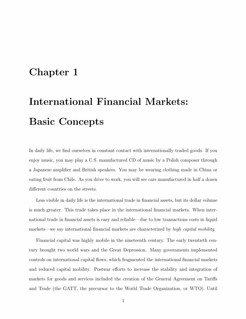
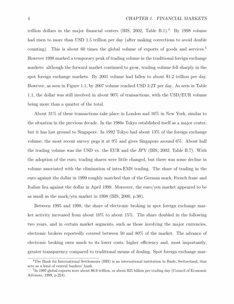
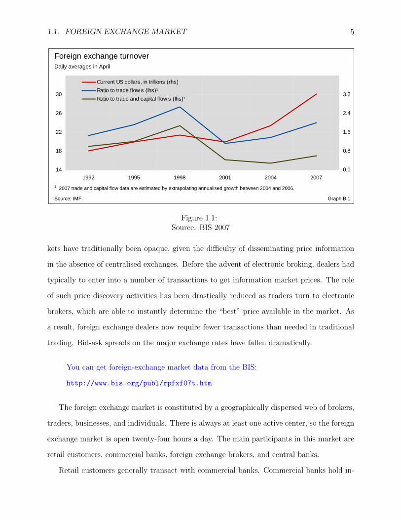
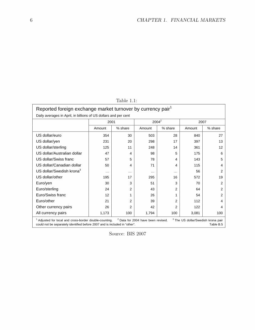
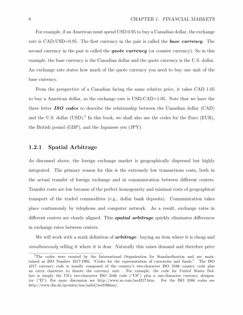
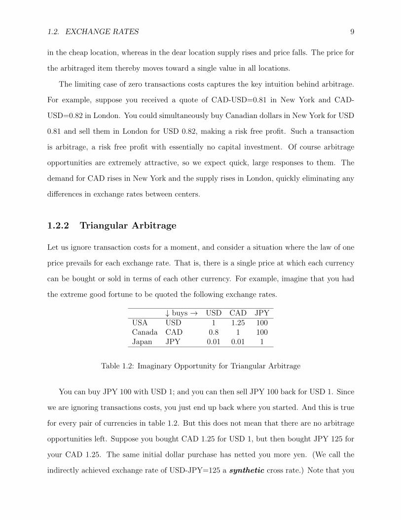
However, as seen in Figure 1.1, by 2007 volume reached USD 3.2T per day. As seen in Table
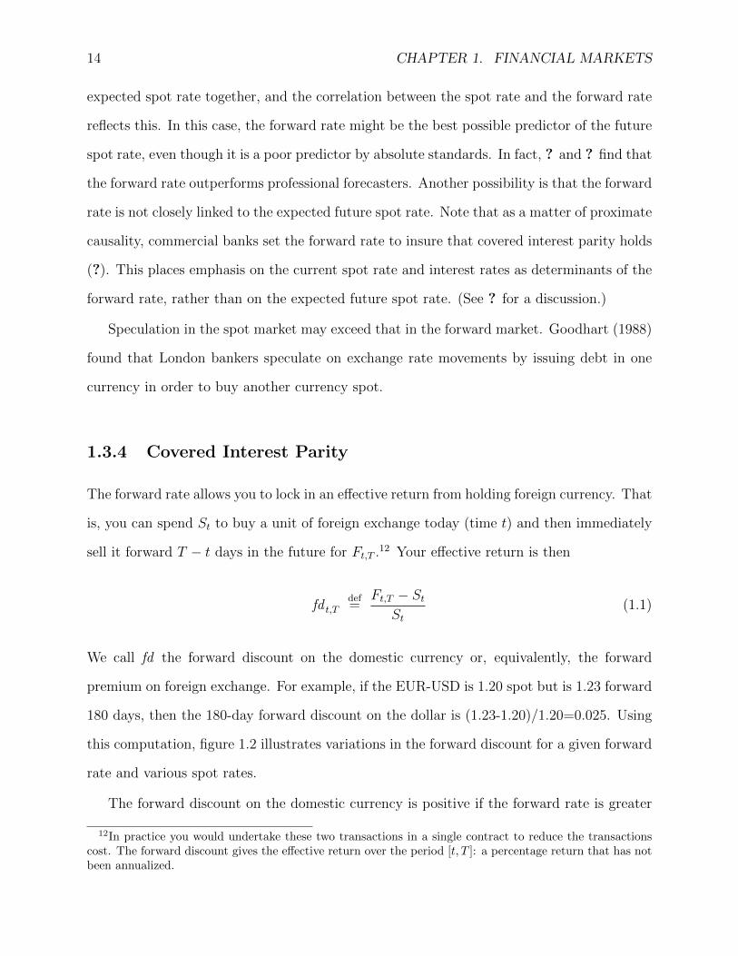
1.1, the dollar was still involved in about 90% of transactions, with the USD/EUR volume
being more than a quarter of the total.
About 31% of these transactions take place in London and 16% in New York, similar to
the situation in the previous decade. In the 1980s Tokyo established itself as a major center,
but it has lost ground to Singapore. In 1992 Tokyo had about 13% of the foreign exchange
volume; the most recent survey pegs it at 9% and gives Singapore around 6%. About half
the trading volume was the USD vs. the EUR and the JPY (BIS, 2002, Table B.7). With
the adoption of the euro, trading shares were little changed, but there was some decline in
volume associated with the elimination of intra-EMS trading. The share of trading in the
euro against the dollar in 1999 roughly matched that of the German mark, French franc and
Italian lira against the dollar in April 1998. Moreover, the euro/yen market appeared to be
as small as the mark/yen market in 1998 (BIS, 2000, p.98).
Between 1995 and 1998, the share of electronic broking in spot foreign exchange mar-
ket activity increased from about 10% to about 15%. The share doubled in the following
two years, and in certain market segments, such as those involving the major currencies,
electronic brokers reportedly covered between 50 and 80% of the market. The advance of
electronic broking owes much to its lower costs, higher efficiency and, most importantly,
greater transparency compared to traditional means of dealing. Spot foreign exchange mar-
4The Bank for International Settlements (BIS) is an international institution in Basle, Switzerland, thatacts as a kind of central bankers’ bank.
5In 1997 global exports were about $6.6 trillion, or about $25 billion per trading day (Council of EconomicAdvisors, 1999, p.224).
1.1. FOREIGN EXCHANGE MARKET 5
Triennial Central Bank Survey 2007 5
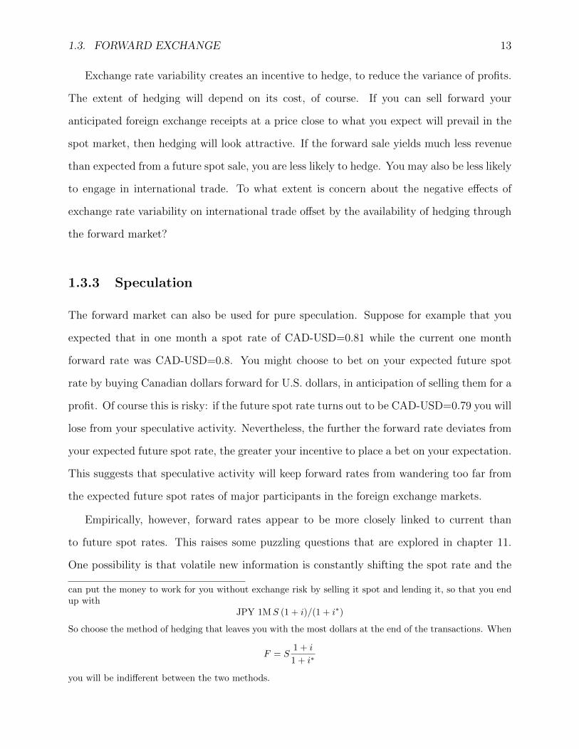
By counterparty, the expansion in turnover in the interbank market was comparable to growth over the previous three years, but was outpaced by the increase recorded in the non-financial customer and non-reporting financial institution segments, which more than doubled in size. The currency composition of foreign exchange turnover became a little more dispersed, with the combined share of the US dollar, the euro and the yen in overall turnover falling.
2. Turnover by counterparty
Half of the growth in aggregate turnover can be attributed to an increase in transactions between reporting dealers and other non-reporting financial institutions, such as non-reporting banks, hedge funds, pension funds and insurance companies (Table B.3). Consequently, the share of this segment increased to 40% from 33%. This growth was broadly based across spot, outright forward and FX swap instruments.
Several factors are likely to have been important for the ongoing strength of turnover growth in this segment.1 Foreign exchange markets have offered investors with short-term horizons relatively attractive risk-adjusted returns over the three years to April 2007, given that exchange rates were broadly trending and financial market volatility was at historically low levels. In addition, there is evidence that longer-term investors, such as pension funds, have contributed to the increase in turnover by systematically diversifying their portfolios internationally.
1 For more details, see G Galati and A Heath, “What drives growth in FX activity? Interpreting
the 2007 triennial survey”, BIS Quarterly Review, December 2007.
Foreign exchange turnover Daily averages in April
0.0
0.8
1.6
2.4
3.2
1992 1995 1998 2001 2004 200714
18
22
26
30
Current US dollars, in trillions (rhs)Ratio to trade f low s (lhs)¹Ratio to trade and capital f low s (lhs)¹
1 2007 trade and capital flow data are estimated by extrapolating annualised growth between 2004 and 2006.
Source: IMF. Graph B.1
Combined share of the main currrencies declined
… underpinned by attractive returns for investors, portfolio diversification …
Tunover with non-reporting financial institutions more than doubled …
Figure 1.1:Source: BIS 2007
kets have traditionally been opaque, given the difficulty of disseminating price information
in the absence of centralised exchanges. Before the advent of electronic broking, dealers had
typically to enter into a number of transactions to get information market prices. The role
of such price discovery activities has been drastically reduced as traders turn to electronic
brokers, which are able to instantly determine the “best” price available in the market. As
a result, foreign exchange dealers now require fewer transactions than needed in traditional
trading. Bid-ask spreads on the major exchange rates have fallen dramatically.
You can get foreign-exchange market data from the BIS:
http://www.bis.org/publ/rpfxf07t.htm
The foreign exchange market is constituted by a geographically dispersed web of brokers,
traders, businesses, and individuals. There is always at least one active center, so the foreign
exchange market is open twenty-four hours a day. The main participants in this market are
retail customers, commercial banks, foreign exchange brokers, and central banks.
Retail customers generally transact with commercial banks. Commercial banks hold in-
6 CHAPTER 1. FINANCIAL MARKETS
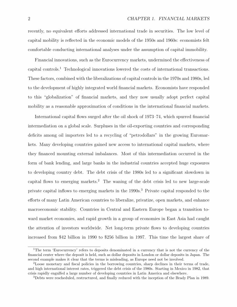
Table 1.1:
10 Triennial Central Bank Survey 2007
In some cases, such as the Australian and New Zealand dollars, the
increase in turnover is likely to partly reflect greater investor activity in high-yielding currencies between 2004 and 2007. For the Chinese renminbi, the Hong Kong dollar and the Indian rupee, the expansion in turnover is likely to be related to strong economic growth and the increasing depth and openness of domestic financial markets in these economies.
More broadly, there appears to have been an increase in the share of emerging market currencies in total turnover: in April 2007, emerging market currencies were involved in almost 20% of all transactions (Table B.6). Emerging market currencies are defined to be the residual when turnover in identified industrialised economy currencies is subtracted from aggregate turnover. This calculation assumes that currencies which are not separately identified4 are emerging market currencies. To the extent that this assumption does not hold exactly, the shares attributed to emerging market currencies in Table B.6 should be treated as upper bounds.
Based on data provided by countries that report on all industrialised economy currencies, it is likely that the degree of overestimation in 2007 is less than 1 percentage point. The degree of overestimation in previous surveys is likely to be larger given that changes implemented for the 2007 triennial survey have allowed for a more comprehensive reporting of currency breakdowns. In particular, changes to reporting forms have made it possible to report offshore trade in industrialised economy currencies more accurately (see Section D.6). For example, it is estimated that this change increased the share of the 4 That is, the residual currency reported in Table E.4.
Reported foreign exchange market turnover by currency pair1 Daily averages in April, in billions of US dollars and per cent
2001 20042 2007 Amount % share Amount % share Amount % share
US dollar/euro 354 30 503 28 840 27
US dollar/yen 231 20 298 17 397 13
US dollar/sterling 125 11 248 14 361 12
US dollar/Australian dollar 47 4 98 5 175 6
US dollar/Swiss franc 57 5 78 4 143 5
US dollar/Canadian dollar 50 4 71 4 115 4
US dollar/Swedish krona3 … … … … 56 2
US dollar/other 195 17 295 16 572 19
Euro/yen 30 3 51 3 70 2
Euro/sterling 24 2 43 2 64 2
Euro/Swiss franc 12 1 26 1 54 2
Euro/other 21 2 39 2 112 4
Other currency pairs 26 2 42 2 122 4
All currency pairs 1,173 100 1,794 100 3,081 100 1 Adjusted for local and cross-border double-counting. 2 Data for 2004 have been revised. 3 The US dollar/Swedish krona pair could not be separately identified before 2007 and is included in “other”. Table B.5
… partly due to investor interest and more open markets
Share of emerging market currencies has increased
Methodology changes have improved the accuracy of these estimates …
Source: BIS 2007
1.2. EXCHANGE RATES 7
ventories of foreign exchange to satisfy the needs of their retail customers. When a retail
customer purchases foreign exchange from a commercial bank, the bank’s inventories of for-
eign exchange are depleted. When the customer sells foreign exchange, the bank’s inventories
increase. If the many retail sales and purchases were perfectly matched, there would be no
net effect on the banks inventories of foreign exchange. But since sales and purchases are
imperfectly offsetting, the bank’s inventories move above or below their desired level. This
is the basis of an active market in foreign exchange among commercial banks.
Commercial banks in the U.S. may trade foreign exchange directly with each other. More
often, they rely on interbank intermediaries called foreign exchange brokers . A broker is
someone who “brings together” a buyer and a seller, without taking a position in foreign
exchange. That is, the broker simply arranges the transaction for a fee. This fee is a spread
between what a purchaser of foreign exchange pays (the ask price) and what the seller of
foreign exchange receives (the bid price).
Use of a foreign exchange broker allows anonymous pricing, which is a reason central
banks also rely on brokers for their foreign exchange transactions. Major brokerage houses
are global and thereby able to service the interbank market around the clock.
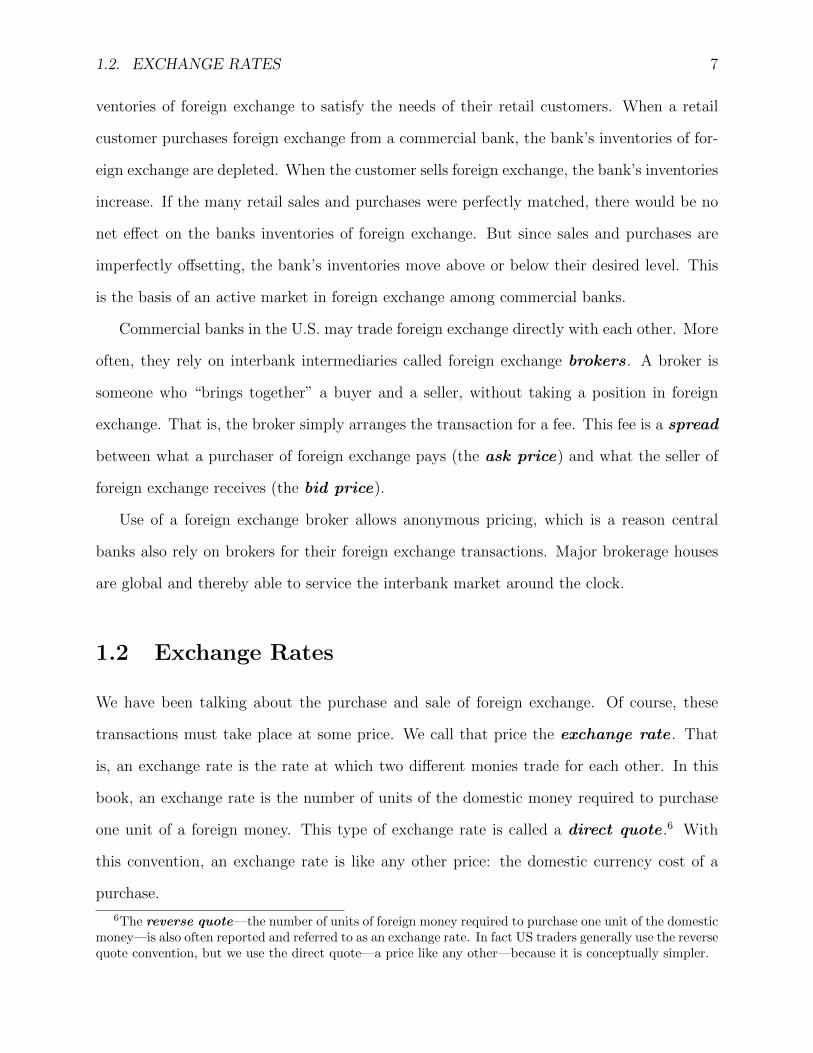
1.2 Exchange Rates
We have been talking about the purchase and sale of foreign exchange. Of course, these
transactions must take place at some price. We call that price the exchange rate . That
is, an exchange rate is the rate at which two different monies trade for each other. In this
book, an exchange rate is the number of units of the domestic money required to purchase
one unit of a foreign money. This type of exchange rate is called a direct quote .6 With
this convention, an exchange rate is like any other price: the domestic currency cost of a
purchase.
6The reverse quote—the number of units of foreign money required to purchase one unit of the domesticmoney—is also often reported and referred to as an exchange rate. In fact US traders generally use the reversequote convention, but we use the direct quote—a price like any other—because it is conceptually simpler.
8 CHAPTER 1. FINANCIAL MARKETS
For example, if an American must spend USD 0.95 to buy a Canadian dollar, the exchange
rate is CAD-USD=0.95. The first currency in the pair is called the base currency . The
second currency in the pair is called the quote currency (or counter currency). So in this
example, the base currency is the Canadian dollar and the quote currency is the U.S. dollar.
An exchange rate states how much of the quote currency you need to buy one unit of the
base currency.
From the perspective of a Canadian facing the same relative price, it takes CAD 1.05
to buy a American dollar, so the exchange rate is USD-CAD=1.05. Note that we have the
three letter ISO codes to describe the relationship between the Canadian dollar (CAD)
and the U.S. dollar (USD).7 In this book, we shall also use the codes for the Euro (EUR),
the British pound (GBP), and the Japanese yen (JPY).
1.2.1 Spatial Arbitrage
As discussed above, the foreign exchange market is geographically dispersed but highly
integrated. The primary reason for this is the extremely low transactions costs, both in
the actual transfer of foreign exchange and in communication between different centers.
Transfer costs are low because of the perfect homogeneity and minimal costs of geographical
transport of the traded commodities (e.g., dollar bank deposits). Communication takes
place continuously by telephone and computer network. As a result, exchange rates in
different centers are closely aligned. This spatial arbitrage quickly eliminates differences
in exchange rates between centers.
We will work with a stark definition of arbitrage : buying an item where it is cheap and
simultaneously selling it where it is dear. Naturally this raises demand and therefore price
7The codes were created by the International Organization for Standardization and are main-tained as ISO Number 4217:1995, “Codes for the representation of currencies and funds.” The ISO4217 currency code is usually composed of the country’s two-character ISO 3166 country code plusan extra character to denote the currency unit. For example, the code for United States Dol-lars is simply the US’s two-character ISO 3166 code (“US”) plus a one-character currency designa-tor (“D”). For more discussion see http://www.xe.com/iso4217.htm. For the ISO 3166 codes seehttp://www.din.de/gremien/nas/nabd/iso3166ma/.
1.2. EXCHANGE RATES 9
in the cheap location, whereas in the dear location supply rises and price falls. The price for
the arbitraged item thereby moves toward a single value in all locations.
The limiting case of zero transactions costs captures the key intuition behind arbitrage.
For example, suppose you received a quote of CAD-USD=0.81 in New York and CAD-
USD=0.82 in London. You could simultaneously buy Canadian dollars in New York for USD
0.81 and sell them in London for USD 0.82, making a risk free profit. Such a transaction
is arbitrage, a risk free profit with essentially no capital investment. Of course arbitrage
opportunities are extremely attractive, so we expect quick, large responses to them. The
demand for CAD rises in New York and the supply rises in London, quickly eliminating any
differences in exchange rates between centers.
1.2.2 Triangular Arbitrage
Let us ignore transaction costs for a moment, and consider a situation where the law of one
price prevails for each exchange rate. That is, there is a single price at which each currency
can be bought or sold in terms of each other currency. For example, imagine that you had
the extreme good fortune to be quoted the following exchange rates.
↓ buys → USD CAD JPYUSA USD 1 1.25 100Canada CAD 0.8 1 100Japan JPY 0.01 0.01 1
Table 1.2: Imaginary Opportunity for Triangular Arbitrage
You can buy JPY 100 with USD 1; and you can then sell JPY 100 back for USD 1. Since
we are ignoring transactions costs, you just end up back where you started. And this is true
for every pair of currencies in table 1.2. But this does not mean that there are no arbitrage
opportunities left. Suppose you bought CAD 1.25 for USD 1, but then bought JPY 125 for
your CAD 1.25. The same initial dollar purchase has netted you more yen. (We call the
indirectly achieved exchange rate of USD-JPY=125 a synthetic cross rate.) Note that you
10 CHAPTER 1. FINANCIAL MARKETS
could now sell your JPY 125 for USD 1.25, completing a triangular arbitrage that nets
you a profit.
As before, we expect that the activity of arbitrageurs will lead to an adjustment of the
exchange rates and an elimination of this profit opportunity. That is, we expect triangular
arbitrage to align exchange rates so that there are no profits from sequentially buying and
selling three currencies. As a result, it is not cheaper to acquire desired foreign currency
indirectly (via a third currency) than directly.
In the absence of triangular arbitrage opportunities, should we consider the profitability
of sequentially buying and selling larger numbers of currencies? The answer is no: the elimi-
nation of triangular arbitrage opportunities also eliminates the profits from longer sequences
of buying and selling.
1.3 Forward Exchange
Up to now, our discussion of the foreign exchange market has focused on the spot rate: the
price for immediate delivery of foreign exchange.8 However it is also possible to use a forward
contract to contract for future sale or purchase of foreign exchange. Like a spot contract, a
forward contract specifies quantity of foreign exchange to be purchased or sold and a price at
which the transaction is to take place. However it also specifies a future date on which the
transaction is to take place. There are active forward markets in major currencies for one
month, two months, three months, 6 months, 9 months, and a year out. Total volume on
the forward exchange markets exceeds that on the spot markets, with most of it occurring
in the one month and three month forward contracts. Spot market purchases have declined
to 40 percent of foreign exchange transactions in 1998, and forward instruments continued
to grow in importance relative to spot sales (Council of Economic Advisors, 1999, p.224).9
8Although small spot transaction may take place with no delay, large spot transactions may allow up totwo working days for delivery (depending on the currencies involved).
9Over-the-counter derivatives remain a small fraction of total transactions, but they have been the fastest-growing segment of the market.
1.3. FORWARD EXCHANGE 11
It is not unusual for banks to quote rates up to ten years forward. The price specified in a
forward contract is referred to as the forward exchange rate.10
Two primary functions of the forward market are hedging and speculation. Hedging is
the purchase or sale of an asset in order to offset the risk involved in one’s current financial
position. For example, someone who expects a future payment in foreign exchange can offset
the implied exchange risk (the risk of an unforeseen change in the spot rate) by selling that
foreign exchange forward. Speculation is the purchase or sale of an asset in order to profit
from the difference between the current value of the asset and its expected future value. For
example, speculators can try to profit from any difference between the current forward rate
and their expectations of the future spot rate. Only about 20% of foreign exchange directly
trades involve nonfinancial customers (Council of Economic Advisors, 1999, p.224).
1.3.1 FX Swaps
You could combine a spot transaction with a forward transaction in the reverse direction.
This locks in a rate of return based on the difference between the two rates. Foreign exchange
swaps allow you to arrange this as a single transaction. For example, foreign exchange may be
purchased spot and sold forward. The combined transaction is detailed in a single contract,
the foreign exchange swap contract, which specifies the term of the swap and the swap rate.
There are two settlement dates: the start date (or “near” date), when the currencies are first
exchanged, and the end date (or “far” date), when they are exchanged back. The difference
between the two exchange rates is called the swap rate (or swap points, if only the final digits
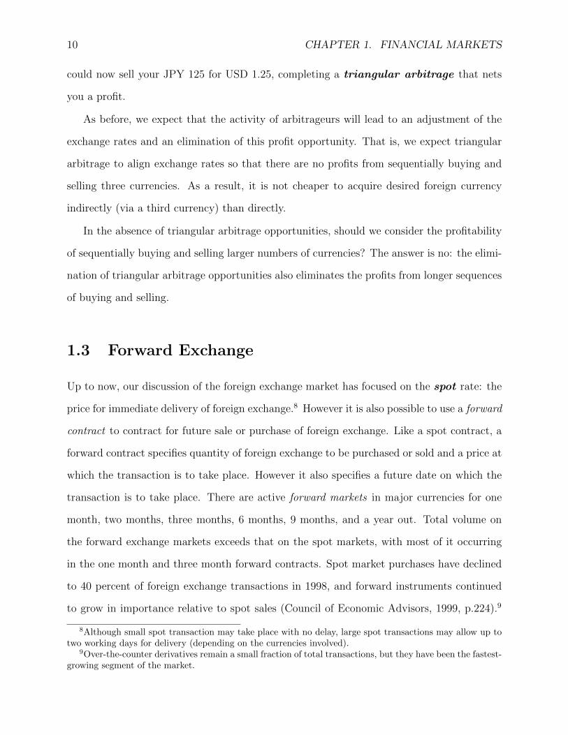
are quoted). For reporting purposes, a swap is considered a single transaction. As seen in
Table 1.3, foreign exchange swaps constitute the bulk of trading in the foreign exchange
market.
10The forward exchange rate is sometimes called the outright rate. Rather than quote the outright rate,market makers may quote the much less volatile swap rate. The swap rate is the difference between theoutright rate and the spot rate. For example, suppose the spot rate is CAD-USD=0.80 spot and you arequoted a swap rate of +0.01. (The CAD is trading at a forward premium.) This implies a forward rate ofCAD-USD=0.81. The swap rate is less volatile than the forward rate because forward and spot rates tendto move together.
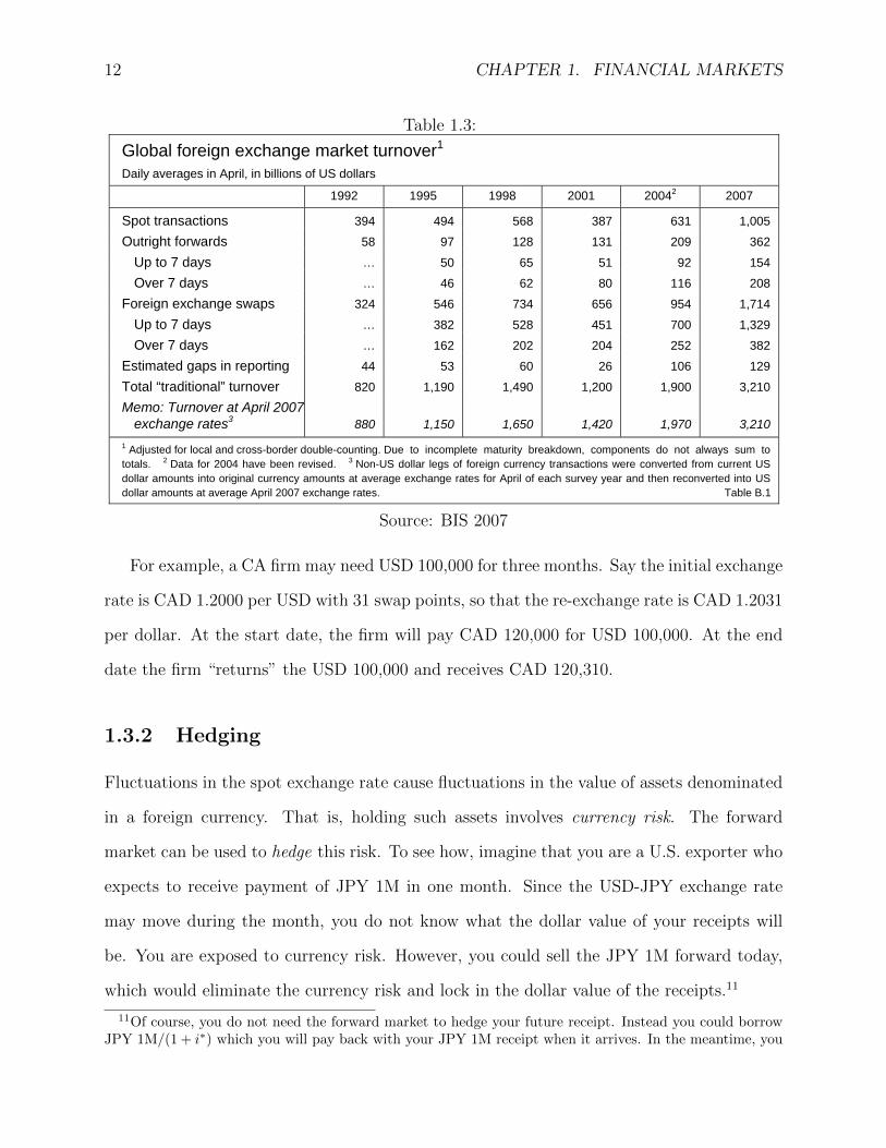
12 CHAPTER 1. FINANCIAL MARKETS
Table 1.3:
4 Triennial Central Bank Survey 2007
B. Traditional foreign exchange markets
1. Global turnover
The 2007 survey shows an unprecedented rise in activity in traditional foreign exchange markets compared to 2004. Average daily turnover rose to $3.2 trillion in April 2007, an increase of 69% at current exchange rates and 63% at constant exchange rates (Table B.1). The ratio of foreign exchange turnover to the value of international trade and capital flows has increased somewhat over the past three years, recovering some of the decline observed in the 2001 triennial survey (Graph B.1).
Growth in turnover was broadly distributed across instruments. The expansion in FX swap turnover was particularly strong and made the largest contribution to aggregate growth. This is in contrast to the period between 2001 and 2004, when growth in FX swaps was significantly lower than that in spot contracts and outright forwards. The share of FX swap transactions accounted for by contracts with a maturity of less than seven days has increased to 78%, from 73% in April 2004, whereas the share of these short-term contracts in outright forward turnover has fallen slightly. In both cases, contracts with a duration exceeding one year command a relatively small share of the total.
The geographical distribution of foreign exchange trading typically changes slowly over time, and the 2007 results are no exception (Table B.2). Among countries with major financial centres, Singapore, Switzerland and the United Kingdom gained market share, while the shares of Japan and the United States dropped. In some cases, changing shares reflected the relocation of desks.
Global foreign exchange market turnover1
Daily averages in April, in billions of US dollars
1992 1995 1998 2001 20042 2007
Spot transactions 394 494 568 387 631 1,005
Outright forwards 58 97 128 131 209 362
Up to 7 days … 50 65 51 92 154
Over 7 days … 46 62 80 116 208
Foreign exchange swaps 324 546 734 656 954 1,714
Up to 7 days … 382 528 451 700 1,329
Over 7 days … 162 202 204 252 382
Estimated gaps in reporting 44 53 60 26 106 129
Total “traditional” turnover 820 1,190 1,490 1,200 1,900 3,210
Memo: Turnover at April 2007 exchange rates3 880 1,150 1,650 1,420 1,970 3,210
1 Adjusted for local and cross-border double-counting. Due to incomplete maturity breakdown, components do not always sum to totals. 2 Data for 2004 have been revised. 3 Non-US dollar legs of foreign currency transactions were converted from current US dollar amounts into original currency amounts at average exchange rates for April of each survey year and then reconverted into US dollar amounts at average April 2007 exchange rates. Table B.1
There was little change in the geographical distribution
… and broadly based across instruments
Growth in global foreign exchange turnover was strong …
Source: BIS 2007
For example, a CA firm may need USD 100,000 for three months. Say the initial exchange
rate is CAD 1.2000 per USD with 31 swap points, so that the re-exchange rate is CAD 1.2031
per dollar. At the start date, the firm will pay CAD 120,000 for USD 100,000. At the end
date the firm “returns” the USD 100,000 and receives CAD 120,310.
1.3.2 Hedging
Fluctuations in the spot exchange rate cause fluctuations in the value of assets denominated
in a foreign currency. That is, holding such assets involves currency risk. The forward
market can be used to hedge this risk. To see how, imagine that you are a U.S. exporter who
expects to receive payment of JPY 1M in one month. Since the USD-JPY exchange rate
may move during the month, you do not know what the dollar value of your receipts will
be. You are exposed to currency risk. However, you could sell the JPY 1M forward today,
which would eliminate the currency risk and lock in the dollar value of the receipts.11
11Of course, you do not need the forward market to hedge your future receipt. Instead you could borrowJPY 1M/(1 + i∗) which you will pay back with your JPY 1M receipt when it arrives. In the meantime, you
1.3. FORWARD EXCHANGE 13
Exchange rate variability creates an incentive to hedge, to reduce the variance of profits.
The extent of hedging will depend on its cost, of course. If you can sell forward your
anticipated foreign exchange receipts at a price close to what you expect will prevail in the
spot market, then hedging will look attractive. If the forward sale yields much less revenue
than expected from a future spot sale, you are less likely to hedge. You may also be less likely
to engage in international trade. To what extent is concern about the negative effects of
exchange rate variability on international trade offset by the availability of hedging through
the forward market?
1.3.3 Speculation
The forward market can also be used for pure speculation. Suppose for example that you
expected that in one month a spot rate of CAD-USD=0.81 while the current one month
forward rate was CAD-USD=0.8. You might choose to bet on your expected future spot
rate by buying Canadian dollars forward for U.S. dollars, in anticipation of selling them for a
profit. Of course this is risky: if the future spot rate turns out to be CAD-USD=0.79 you will
lose from your speculative activity. Nevertheless, the further the forward rate deviates from
your expected future spot rate, the greater your incentive to place a bet on your expectation.
This suggests that speculative activity will keep forward rates from wandering too far from
the expected future spot rates of major participants in the foreign exchange markets.
Empirically, however, forward rates appear to be more closely linked to current than
to future spot rates. This raises some puzzling questions that are explored in chapter 11.
One possibility is that volatile new information is constantly shifting the spot rate and the
can put the money to work for you without exchange risk by selling it spot and lending it, so that you endup with
JPY 1MS (1 + i)/(1 + i∗)
So choose the method of hedging that leaves you with the most dollars at the end of the transactions. When
F = S1 + i
1 + i∗
you will be indifferent between the two methods.
14 CHAPTER 1. FINANCIAL MARKETS
expected spot rate together, and the correlation between the spot rate and the forward rate
reflects this. In this case, the forward rate might be the best possible predictor of the future
spot rate, even though it is a poor predictor by absolute standards. In fact, ? and ? find that
the forward rate outperforms professional forecasters. Another possibility is that the forward
rate is not closely linked to the expected future spot rate. Note that as a matter of proximate
causality, commercial banks set the forward rate to insure that covered interest parity holds
(?). This places emphasis on the current spot rate and interest rates as determinants of the
forward rate, rather than on the expected future spot rate. (See ? for a discussion.)
Speculation in the spot market may exceed that in the forward market. Goodhart (1988)
found that London bankers speculate on exchange rate movements by issuing debt in one
currency in order to buy another currency spot.
1.3.4 Covered Interest Parity
The forward rate allows you to lock in an effective return from holding foreign currency. That
is, you can spend St to buy a unit of foreign exchange today (time t) and then immediately
sell it forward T − t days in the future for Ft,T .12 Your effective return is then
fd t,Tdef=
Ft,T − St
St
(1.1)
We call fd the forward discount on the domestic currency or, equivalently, the forward
premium on foreign exchange. For example, if the EUR-USD is 1.20 spot but is 1.23 forward
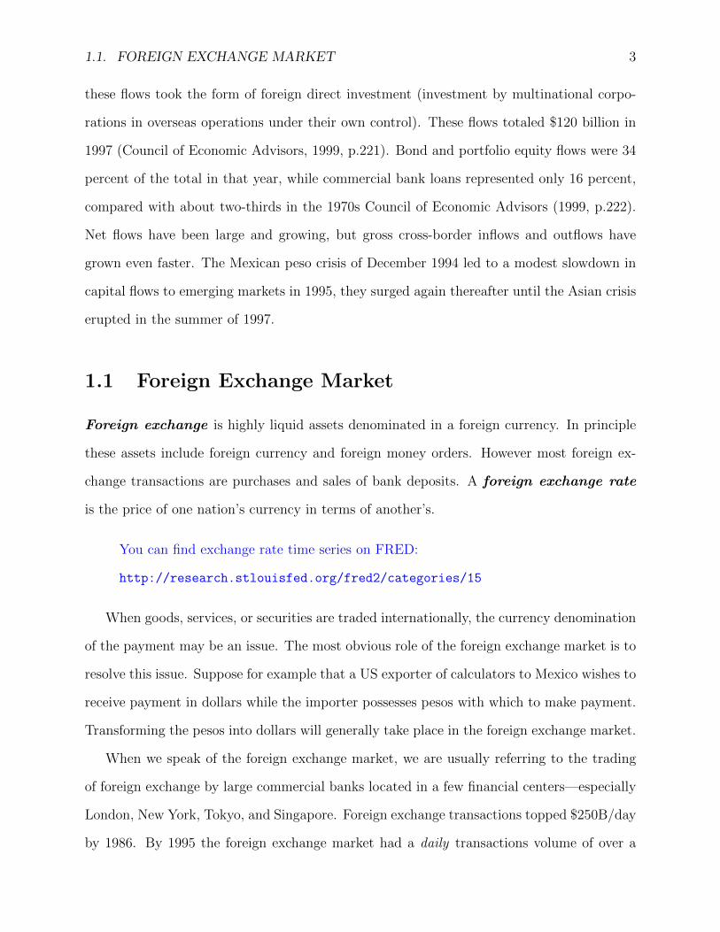
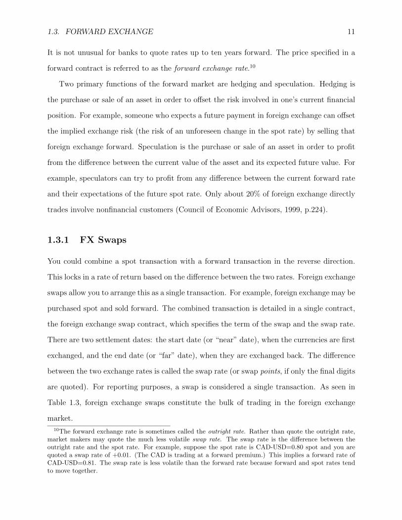
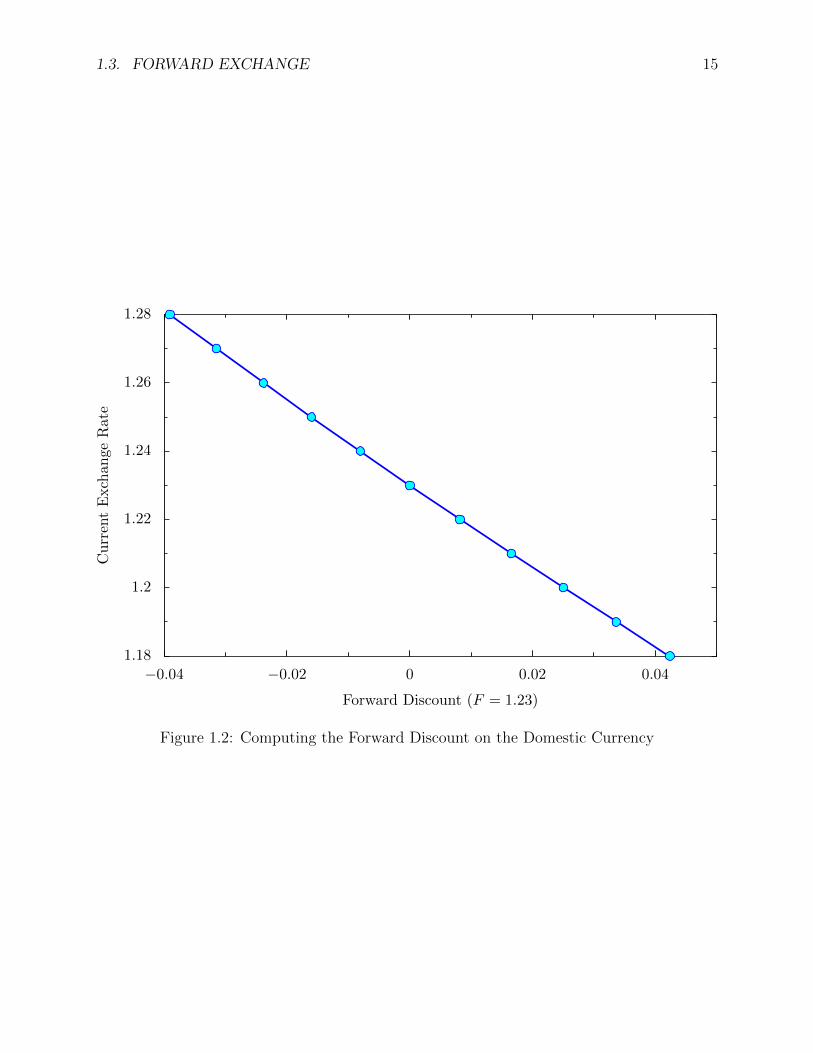
180 days, then the 180-day forward discount on the dollar is (1.23-1.20)/1.20=0.025. Using
this computation, figure 1.2 illustrates variations in the forward discount for a given forward
rate and various spot rates.
The forward discount on the domestic currency is positive if the forward rate is greater
12In practice you would undertake these two transactions in a single contract to reduce the transactionscost. The forward discount gives the effective return over the period [t, T ]: a percentage return that has notbeen annualized.
1.3. FORWARD EXCHANGE 15
1.18
1.2
1.22
1.24
1.26
1.28
CurrentExchan
geRate
−0.04 −0.02 0 0.02 0.04
Forward Discount (F = 1.23)
Figure 1.2: Computing the Forward Discount on the Domestic Currency
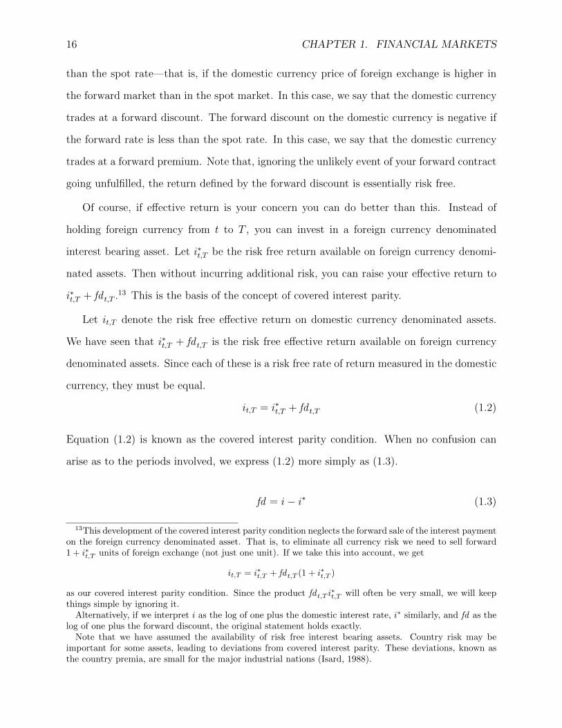
16 CHAPTER 1. FINANCIAL MARKETS
than the spot rate—that is, if the domestic currency price of foreign exchange is higher in
the forward market than in the spot market. In this case, we say that the domestic currency
trades at a forward discount. The forward discount on the domestic currency is negative if
the forward rate is less than the spot rate. In this case, we say that the domestic currency
trades at a forward premium. Note that, ignoring the unlikely event of your forward contract
going unfulfilled, the return defined by the forward discount is essentially risk free.
Of course, if effective return is your concern you can do better than this. Instead of
holding foreign currency from t to T , you can invest in a foreign currency denominated
interest bearing asset. Let i∗t,T be the risk free return available on foreign currency denomi-
nated assets. Then without incurring additional risk, you can raise your effective return to
i∗t,T + fd t,T .13 This is the basis of the concept of covered interest parity.
Let it,T denote the risk free effective return on domestic currency denominated assets.
We have seen that i∗t,T + fd t,T is the risk free effective return available on foreign currency
denominated assets. Since each of these is a risk free rate of return measured in the domestic
currency, they must be equal.
it,T = i∗t,T + fd t,T (1.2)
Equation (1.2) is known as the covered interest parity condition. When no confusion can
arise as to the periods involved, we express (1.2) more simply as (1.3).
fd = i− i∗ (1.3)
13This development of the covered interest parity condition neglects the forward sale of the interest paymenton the foreign currency denominated asset. That is, to eliminate all currency risk we need to sell forward1 + i∗t,T units of foreign exchange (not just one unit). If we take this into account, we get
it,T = i∗t,T + fd t,T (1 + i∗t,T )
as our covered interest parity condition. Since the product fd t,T i∗t,T will often be very small, we will keep
things simple by ignoring it.Alternatively, if we interpret i as the log of one plus the domestic interest rate, i∗ similarly, and fd as the
log of one plus the forward discount, the original statement holds exactly.Note that we have assumed the availability of risk free interest bearing assets. Country risk may be
important for some assets, leading to deviations from covered interest parity. These deviations, known asthe country premia, are small for the major industrial nations (Isard, 1988).
1.3. FORWARD EXCHANGE 17
We say portfolio capital is “mobile” to the extent that international financial markets
are frictionlessly integrated. (Frictions include transactions costs or government controls.)
In such circumstance, domestic and foreign residents are on equal footing in the purchase
and sale of domestic and foreign assets. We then expect opportunities for risk-free profit
making—arbitrage opportunities—to be quickly and completely exploited. Thus the most
basic measure of international capital mobility is the disappearance of arbitrage opportunities
in international financial markets. Of particular interest for our current purposes is that
different ways of obtaining a riskless interest yield in any one currency should yield identical
rates of return. That is, covered interest parity should obtain. Covered interest parity is
thus a basic condition of perfect capital mobility, and deviations from covered interest parity
are a primary indicator of imperfections or frictions in international capital markets.
Deviations from covered interest parity can be due to transactions costs, capital controls,
political risk (e.g., fear of capital controls), or limitations on the supply of arbitrage funds.
The last of these may help explain why CIP does not appear to hold well over long horizons
(e.g., several years). Political-risk is sometimes discussed under the rubric of ‘safe-haven
effects,’ where an increase in perceived political risk leads to an increased demand for assets
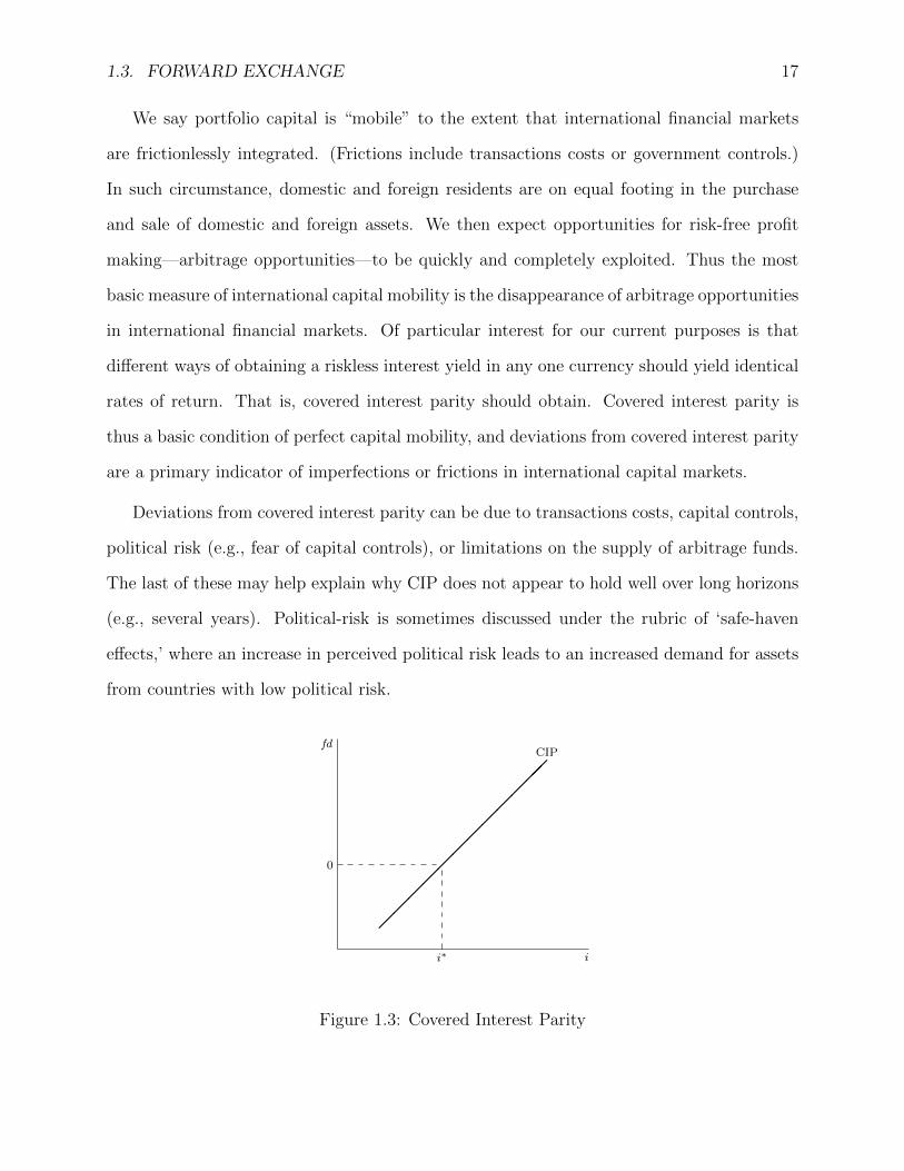
from countries with low political risk.
fd
i
0
i∗
��
��
��
���
���
CIP
Figure 1.3: Covered Interest Parity
18 CHAPTER 1. FINANCIAL MARKETS
1.4 Capital Mobility
When financial assets are freely tradable across international borders at negligeable trans-
actions costs, we speak of perfect capital mobility. For many countries, especially developed
economies, perfect capital mobility seems to be a reasonable approximation of actual market
conditions. Yet in a world with highly integrated financial markets, we might expect returns
on similar domestic and foreign assets (Harberger, 1978). Returns on domestic and foreign
assets often differ, even when the assets appear comparable in risk and liquidity character-
istics.14 In this section, we briefly explore three reasons for this divergence: risk premia,
transactions costs, and capital controls.
1.4.1 Risk Premium
Even economies with perfect capital mobility may not have perfect capital substitutability.
An individual treats two assets as perfect substitutes when the decision between them is
based solely on their expected rate of return. An immediate implication is that when market
participants consider two assets to be perfect substitutes, these will offer a common expected
rate of return. Most assets, however, are not perfectly substitutable in an individual’s
portfolio. For example, an individual will usually care about the risk characteristics of
assets, which generally differ among assets. (See chapter 11 for a more complete discussion.)
Compare the ex post real return from holding the domestic asset, with the uncovered real
return from holding the foreign asset,
rtdef= it − πt+1 (1.4)
rdftdef= i∗t + ∆st+1 − πt+1 (1.5)
14Furthermore, domestic savings and investment are highly correlated, which is something of a puzzle inhighly integrated financial markets (Feldstein and Horioka, 1980; Frankel, 1991). However, Montiel (1994)notes that Feldstein-Horioka tests indicate a relatively high degree of capital mobility for most Latin Americancountries, despite the extensive legal barriers.
1.4. CAPITAL MOBILITY 19
Define the excess return on the domestic asset as difference between these two ex post real
rates of return.
er t+1def= rt − rdftdef= (it − πt+1)− (i∗t + ∆st+1 − πt+1)
= it − (i∗t + ∆st+1)
(1.6)
This is the ex post difference in the uncovered returns.
A similar relationship must hold for the expected excess returns and the expected rate
of depreciation of the spot rate. Consider an individual facing interest rates i and i∗ who
expects the spot rate depreciation to be ∆se. If this individual understands (1.6) and has a
minimal consistency in her expectations, then her expected excess return from holding the
domestic asset with interest rate i instead of the foreign asset with interest rate i∗ must be
er et+1 = it − (i∗t + ∆set+1) (1.7)
A key determinant of an individual’s asset allocation decisions will be the expected excess
return from holding that asset. (We discuss this in detail in chapter 11.) We refer to the
equilibrium expected excess return as the risk premium (rp) in the foreign exchange market.
For convenience we will ignore any variation in the spot depreciation expected by different
market participants, so we can just write the risk premium without ambiguity.
rptdef= er e
t+1
= it − (i∗t + ∆set+1)
(1.8)
In an efficient market , the expectations of market participants are fully reflected in
the equilibrium market price. That is, we call a market efficient when the market price
is an equilibrium price that fully reflects the beliefs of market participants. When capital
is highly mobile, we expect the foreign exchange markets to be very efficient in this sense.
20 CHAPTER 1. FINANCIAL MARKETS
In the example we are considering, interest rates will fully reflect the spot rate depreciation
expected by market participants (since this determines their expected excess returns and
thereby their asset demands). Capital mobility will also assure covered interest parity, so we
can also express the risk premium as
rpt = fd t −∆set+1 (1.9)
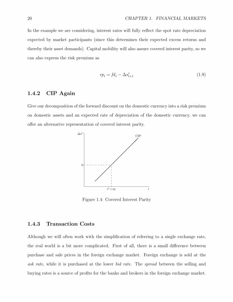
1.4.2 CIP Again
Give our decomposition of the forward discount on the domestic currency into a risk premium
on domestic assets and an expected rate of depreciation of the domestic currency, we can
offer an alternative representation of covered interest parity.
∆se
i
0
i∗+rp
��
���
���
����
CIP
Figure 1.4: Covered Interest Parity
1.4.3 Transaction Costs
Although we will often work with the simplification of referring to a single exchange rate,
the real world is a bit more complicated. First of all, there is a small difference between
purchase and sale prices in the foreign exchange market. Foreign exchange is sold at the
ask rate, while it is purchased at the lower bid rate. The spread between the selling and
buying rates is a source of profits for the banks and brokers in the foreign exchange market.
1.4. CAPITAL MOBILITY 21
£0 £1
$0 $1
-�
6
?
-�
6
?
(1 + tS)S (1 + tS)/S
(1 + t∗)(1 + i∗)
(1 + t∗)/(1 + i∗)
(1 + tF )F (1 + tF )/F
(1 + t)(1 + i)
(1 + t)/(1 + i)
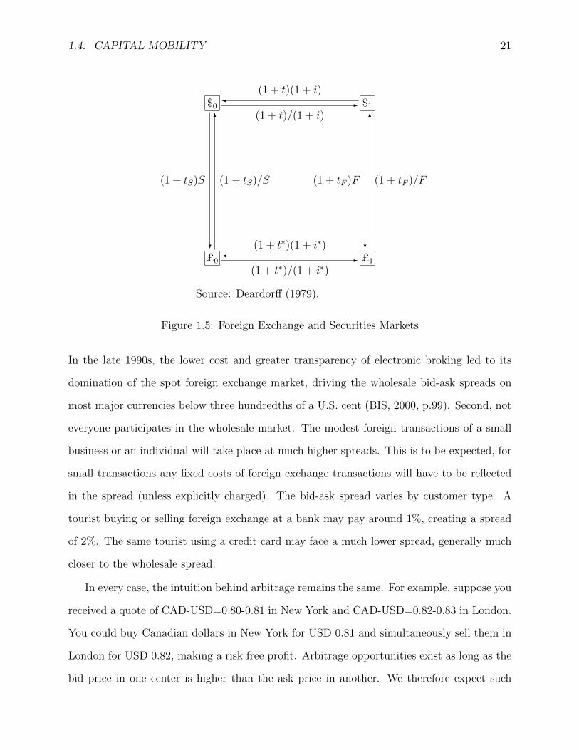
Source: Deardorff (1979).
Figure 1.5: Foreign Exchange and Securities Markets
In the late 1990s, the lower cost and greater transparency of electronic broking led to its
domination of the spot foreign exchange market, driving the wholesale bid-ask spreads on
most major currencies below three hundredths of a U.S. cent (BIS, 2000, p.99). Second, not
everyone participates in the wholesale market. The modest foreign transactions of a small
business or an individual will take place at much higher spreads. This is to be expected, for
small transactions any fixed costs of foreign exchange transactions will have to be reflected
in the spread (unless explicitly charged). The bid-ask spread varies by customer type. A
tourist buying or selling foreign exchange at a bank may pay around 1%, creating a spread
of 2%. The same tourist using a credit card may face a much lower spread, generally much
closer to the wholesale spread.
In every case, the intuition behind arbitrage remains the same. For example, suppose you
received a quote of CAD-USD=0.80-0.81 in New York and CAD-USD=0.82-0.83 in London.
You could buy Canadian dollars in New York for USD 0.81 and simultaneously sell them in
London for USD 0.82, making a risk free profit. Arbitrage opportunities exist as long as the
bid price in one center is higher than the ask price in another. We therefore expect such
22 CHAPTER 1. FINANCIAL MARKETS
occurrences to quickly disappear.
Competition and the Law of One Price
You may have noticed that in the presence of transaction costs the arbitrage argument does
not assure that bid prices (or ask prices) are identical across centers. Arbitrage merely
assures that bid and ask prices overlap. However we can expect identical bid and ask prices
across centers due to the competition among traders in the foreign exchange markets. Any
bank wishing to sell foreign exchange must offer it at a price as low as that of its competitors.
Any bank wishing to buy foreign exchange must offer a price as high as its competitors. Thus
all banks who wish to be involved in both buying and selling foreign exchange will have the
same bid and ask prices.
Synthetic Cross Rates
Once we return to the consideration of transactions costs, synthetic cross rates may be
preferable to direct rates despite triangular arbitrage. Essentially, a synthetic version of
a contract relies on multiple transactions to achieve the goal of the contract. Clearly the
transactions costs of multiple transactions will be an issue in the construction of synthetic
contracts. Yet moving between two currencies can be cheapest using the U.S. dollar as an
intermediary, despite the need to incur transactions costs twice. The reason is that the high
trading volume in the U.S. dollar results in low spreads of the U.S. dollar against other
currencies.
Although there are an increasing number of exceptions, most currencies simply are not
traded against each other by professional traders. Even the most actively traded currencies
tend to be traded against the dollar. Suppose we have twenty actively traded currencies;
then each will have nineteen exchange rates. That is 380 prices to keep track of in the foreign
exchange markets. But if all twenty currencies are always quoted against the dollar, there
are only nineteen prices to keep track of. At the retail level, the background reliance on the
1.4. CAPITAL MOBILITY 23
dollar is invisible: the customer is simply quoted the cross-rate.
1.4.4 Capital Controls
Capital controls were common in the twentieth century. The use of capital controls surged
during World War I and again during the Great Depression. After World War II, many
countries continued to use capital controls in an effort to deal with balance-of-payments
difficulties. The IMF explicitly permitted such controls.15
During the 1970s and 1980s, the developed countries removed most of their controls on the
international trade in financial assets. The free flow of international capital was presumed to
increase income and growth, and developing countries were encouraged to follow suit. In the
1990s, many developing countries nevertheless continued to rely on extensive capital controls,
often as a way to insulate their macroeconomic policy from international considerations
(Grilli and Milesi-Ferretti, 1995; Johnston and Tamirisa, 1998). Controls on capital outflows
were the most prevalent. But countries also turned to controls on capital inflows, primarily
to control direct foreign investment and real estate purchases (Johnston and Tamirisa, 1998).
Latin American countries in particular, and especially Chile and Colombia, turned to controls
on capital inflows in an attempt to slow large capital inflows (Edwards, 1998).
Capital flows are one way to move consumption between the present and the future, and
there can be many good reasons to do this. Demographic shifts are one reason: an aging
population may find it prudent to save for retirement by investing abroad. This may explain
why the more rapidly aging Japanese population buys more assets from the U.S. than they
sell there (Neely, 1999). Real investment opportunities are another reason. It can pay to
borrow abroad in order to make high yielding domestic investments. For example, from
1960–1980 South Korea borrowed heavily in international markets, financing its domestic
investments during a period of strong growth (Neely, 1999). Finally, it may pay to borrow
15Consider the following section of the IMF’s Articles of Agreement, signed in 1944. “Article VI. Section 3.Controls of capital transfers: members may exercise such controls as are necessary to regulate internationalcapital movements . . . ”
24 CHAPTER 1. FINANCIAL MARKETS
in order to consume in the face of temporary negative real-income shocks, including declines
in export prices, rises in import prices, recession, or natural disasters. For example, after
a devastating earthquake in 1980, Italy borrowed abroad to help finance disaster relief and
rebuilding (Neely, 1999). These examples highlight the benefits of international capital flows.
However in the 1990s, a series of financial crises diminished the reputation of capital
flows. In 1992–3, the European Monetary System. In December 1994, after a decade of
reforms had finally led to renewed confidence and large capital inflows, Mexico experienced
a major currency crisis. In 1997–8, several East Asian economies experienced large capital
outflows that forced abandonment of exchange rate pegs and precipitated banking crises and
severe recessions. As policy makers searched for ways to prevent a recurrence of such crises,
many focused on the benefits of limiting the mobility of financial capital. On September 1,
1998, Malaysia adopted capital controls. The Malaysian strategy was to discourage short-
term capital flows while permitting long-term capital to flow freely. Early assessments of
the results were largely favorable, although some observers worried that they were replacing
rather than enabling reform of a fragile financial sector (Neely, 1999).
Speculative Attacks
In 1997, government policies in Thailand led to high nominal interest rates and a stock
market decline. Currency traders began to question whether the central bank could sustain
these policies and whether a devaluation of the baht was imminent. High capital mobility
meant that these speculators could rapidly move huge sums in order to place their bets
against the baht. George Soros, a famous currency speculator who had profited handsomely
from the collapse of the British pound in 1992, began with others to bet heavily against
the baht. In May, trading soared from the usual USD 1B/day to more than USD 10B/day.
Other Asian central banks aided the Thai central bank in its defense of the baht, and initially
Soros and other traders left the field with huge losses. Ultimately, however, the speculators
proved correct in their anticipation that the baht parity could not be sustained.
Terms and Concepts
arbitrage, 7
spatial, 7
triangular, 7, 8
ask price, 5
ask rate, 18
base currency, 6
bid price, 5
bid rate, 18
bid-ask spread, 18
capital mobility
high, 1
perfect, 15
capital substitutability
perfect, 16
covered interest parity, 12
cross rate
synthetic, 8
direct quote, 6
efficient markets, 17
hypothesis, 35
Eurocurrency, 2
excess return, 16
exchange rate, 6
forward, 9
spot, 9
swap, 9
synthetic, 20
forecast error, 33
Foreign exchange, 3
foreign exchange
brokers, 5
defined, 3
market, 3
foreign exchange rate, 3
forward discount, 12
forward premium, see forward discount
forward rate, see exchange rate, forward
hedging, 10
ISO codes, 6
law of iterated expectations, 34
parity
interest
25
26 TERMS AND CONCEPTS
covered, see covered interest parity
quote currency, 6
reverse quote, 6
risk premium, 17
spatial arbitrage, 7
speculation, 11
spot rate, see exchange rate, spot
spread, 5, 18
triangular arbitrage, 8
TERMS AND CONCEPTS 27
Problems for Review
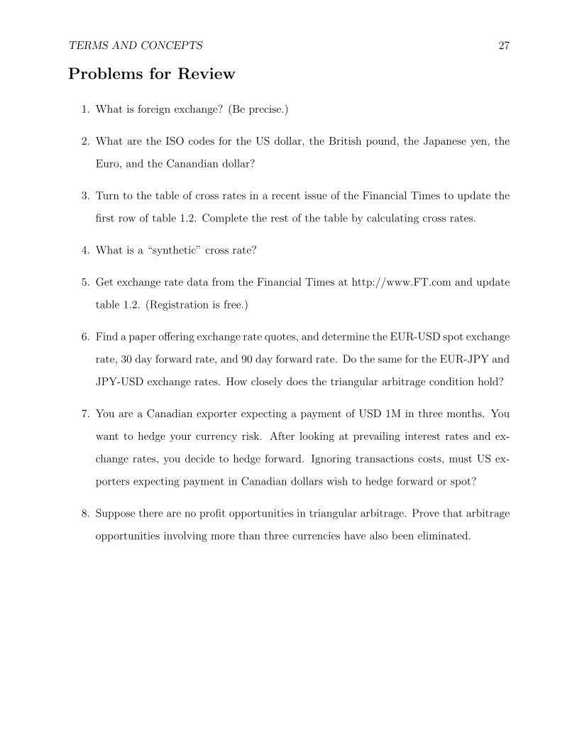
1. What is foreign exchange? (Be precise.)
2. What are the ISO codes for the US dollar, the British pound, the Japanese yen, the
Euro, and the Canandian dollar?
3. Turn to the table of cross rates in a recent issue of the Financial Times to update the
first row of table 1.2. Complete the rest of the table by calculating cross rates.
4. What is a “synthetic” cross rate?
5. Get exchange rate data from the Financial Times at http://www.FT.com and update
table 1.2. (Registration is free.)
6. Find a paper offering exchange rate quotes, and determine the EUR-USD spot exchange
rate, 30 day forward rate, and 90 day forward rate. Do the same for the EUR-JPY and
JPY-USD exchange rates. How closely does the triangular arbitrage condition hold?
7. You are a Canadian exporter expecting a payment of USD 1M in three months. You
want to hedge your currency risk. After looking at prevailing interest rates and ex-
change rates, you decide to hedge forward. Ignoring transactions costs, must US ex-
porters expecting payment in Canadian dollars wish to hedge forward or spot?
8. Suppose there are no profit opportunities in triangular arbitrage. Prove that arbitrage
opportunities involving more than three currencies have also been eliminated.

28 TERMS AND CONCEPTS
Bibliography
BIS (2000). 70th Annual Report. Basle: Bank for International Settlements.
BIS (2002, March). Triennial Central Bank Survey: Foreign Exchange and Derivatives
Market Activity in 2001. Basle: Bank for International Settlements.
Council of Economic Advisors (1999, February). Economic Report of the President. Wash-
ington, DC: United States Government Printing Office.
Deardorff, A. V. (1979, April). “One-way Arbitrage and Its Implications for the Foreign
Exchange Markets.” Journal of Political Economy 87(2), 351–64.
Edwards, Sebastian (1998). “Capital Flows, Real Exchange Rates, and Capital Controls:
Some Latin American Experiences.” NBER Working Paper 6800, National Bureau of
Economic Research.
Fama, Eugene F. (1970). “Efficient Capital Markets: A Review of Theory and Empirical
Work.” Journal of Finance 25, 383–417.
Feldstein, Martin and Charles Horioka (1980, June). “Domestic Saving and International
Capital Flows.” Economic Journal 90(358), 314–29.
Frankel, Jeffery A. (1991). “Quantifying International Capital Mobility in the 1980s.” In
D. Bernheim and J. Shoven, eds., National Saving and Economic Performance, pp. 227–60.
Chicago: University of Chicago Press. As reprinted in Frankel (1997).
29
30 BIBLIOGRAPHY
Frankel, Jeffery A. (1997). On Exchange Rates. Cambridge, Massachusetts: The MIT Press.
Goodhart, Charles A. E. (1988, November). “The Foreign Exchange Market: A Random
Walk with a Dragging Anchor.” Economica 55(220), 437–460.
Grilli, Vittorio and Gian Maria Milesi-Ferretti (1995, September). “Economic Effects and
Structural Determinants of Capital Flows.” International Monetary Fund Staff Pa-
pers 42(3), 517–51.
Harberger, Arnold (1978). “Perspectives on Capital and Technology in Less Developed
Countries.” In M. Artis and A. Nobay, eds., Contemporary Economic Analysis, pp. 151–
69. Lodon: Croom Helm.
Isard, Peter (1988). “Exchange Rate Modeling: An Assessment of Alternative Approaches.”
In Ralph C. Bryant, Dale W. Henderson, Gerald Holtham, Peter Hooper, and Steven A.
Symansky, eds., Empirical Macroeconomics for Interdependent Economies, Chapter 8, pp.
183–201. Washington, D.C.: The Brookings Institution.
Johnston, R. Barry and Natalia T. Tamirisa (1998, December). “Why Do Countries Use Cap-
ital Controls?” IMF Working Paper 98/181, International Monetary Fund, Washington,
DC.
Maor, Eli (1994). e: The Story of a Number. Princeton, NJ: Princeton University Press.
Montiel, Peter J. (1994, September). “Capital Mobility in Developing Countries: Some
Measurement Issues and Empirical Estimates.” The World Bank Economic Review 8(3),
311–50.
Neely, Christopher J. (1999, Nov./Dec.). “An Introduction to Capital Controls.” Federal
Reserve Bank of St. Louis Review 81(6), 13–30.
.1. EXPONENTS AND LOGARITHMS 31
.1 Exponents and Logarithms
In order to test whether the available data are supportive of the core predictions of the
monetary approach, we often need to specify the functional form of relationships that we
have been describing only in the most general theoretical terms. Many empirical tests of the
monetary approach require us to be specific about the functional form for money demand.
The most widely used functional form is log-linear. This section offers a very brief review of
logarithms. (The next section develops the log-linear specification of the monetary approach
to the determination of flexible exchange rates.)
The discussion in this section is indebted to Maor (1994).
The simplest way to motivate logarithms is by thinking again about the geometric pro-
gression 20, 21, 22, . . . . The monotonicity of the exponential function means that it is an
injection (one-to-one), so that the inverse mapping is also a function. We call the inverse
mapping the logarithmic function. Continuing with our base 2 example, the exponential
function maps 2 7→ 4 and 3 7→ 8, so the logarithmic function maps 4 7→ 2 and 8 7→ 3.
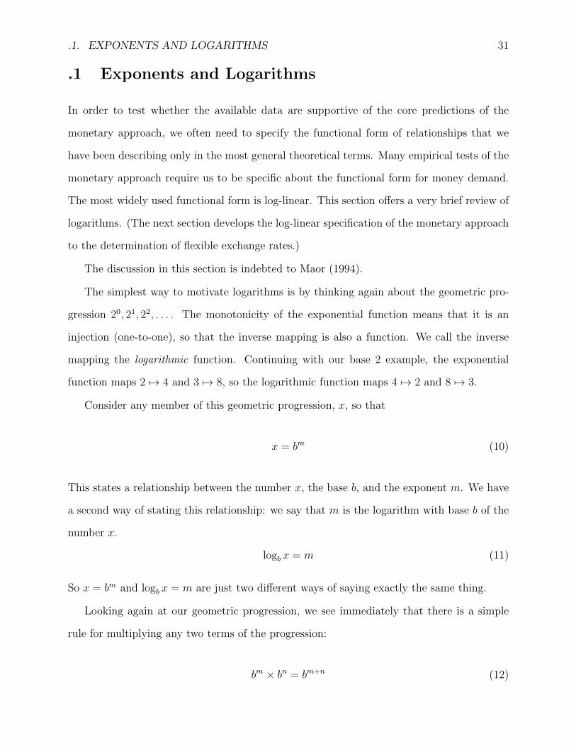
Consider any member of this geometric progression, x, so that
x = bm (10)
This states a relationship between the number x, the base b, and the exponent m. We have
a second way of stating this relationship: we say that m is the logarithm with base b of the
number x.
logb x = m (11)
So x = bm and logb x = m are just two different ways of saying exactly the same thing.
Looking again at our geometric progression, we see immediately that there is a simple
rule for multiplying any two terms of the progression:
bm × bn = bm+n (12)
32 BIBLIOGRAPHY
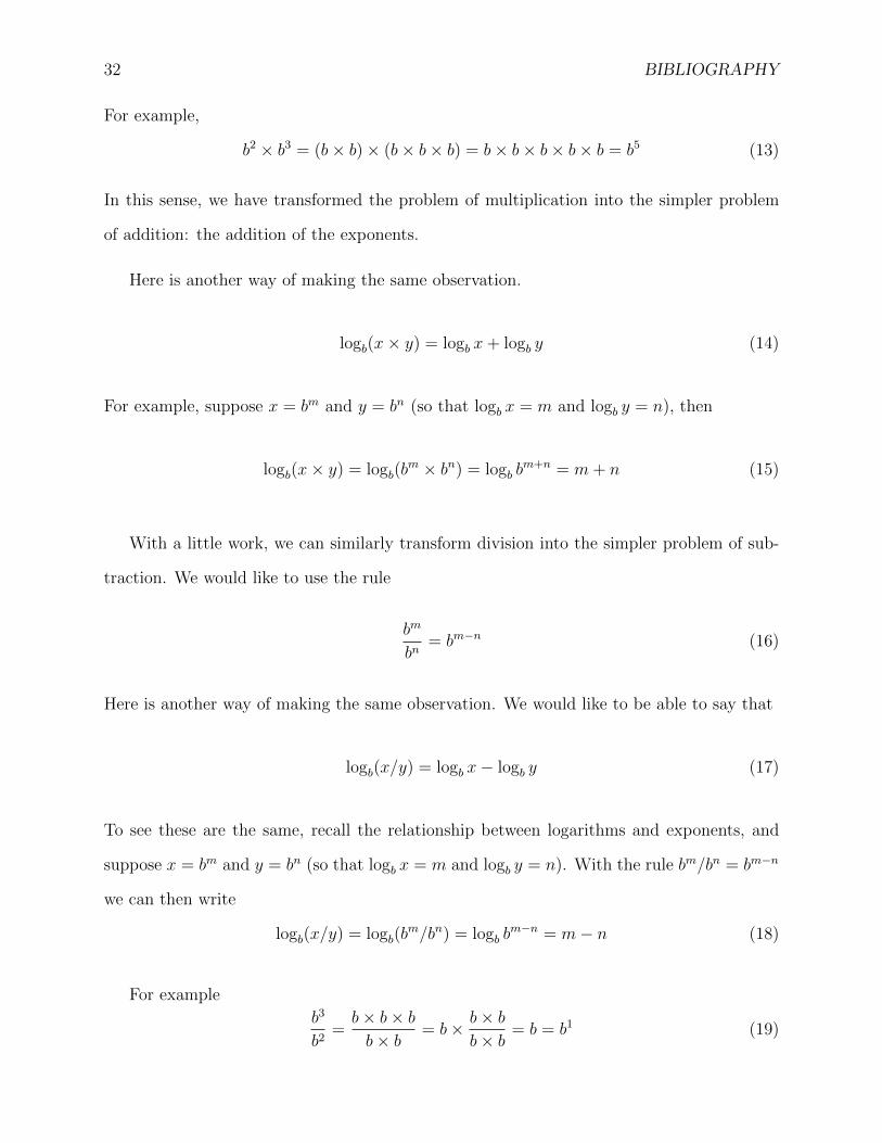
For example,
b2 × b3 = (b× b)× (b× b× b) = b× b× b× b× b = b5 (13)
In this sense, we have transformed the problem of multiplication into the simpler problem
of addition: the addition of the exponents.
Here is another way of making the same observation.
logb(x× y) = logb x+ logb y (14)
For example, suppose x = bm and y = bn (so that logb x = m and logb y = n), then
logb(x× y) = logb(bm × bn) = logb b
m+n = m+ n (15)
With a little work, we can similarly transform division into the simpler problem of sub-
traction. We would like to use the rule
bm
bn= bm−n (16)
Here is another way of making the same observation. We would like to be able to say that
logb(x/y) = logb x− logb y (17)
To see these are the same, recall the relationship between logarithms and exponents, and
suppose x = bm and y = bn (so that logb x = m and logb y = n). With the rule bm/bn = bm−n
we can then write
logb(x/y) = logb(bm/bn) = logb b
m−n = m− n (18)
For example
b3
b2=b× b× bb× b = b× b× b
b× b = b = b1 (19)
.1. EXPONENTS AND LOGARITHMS 33
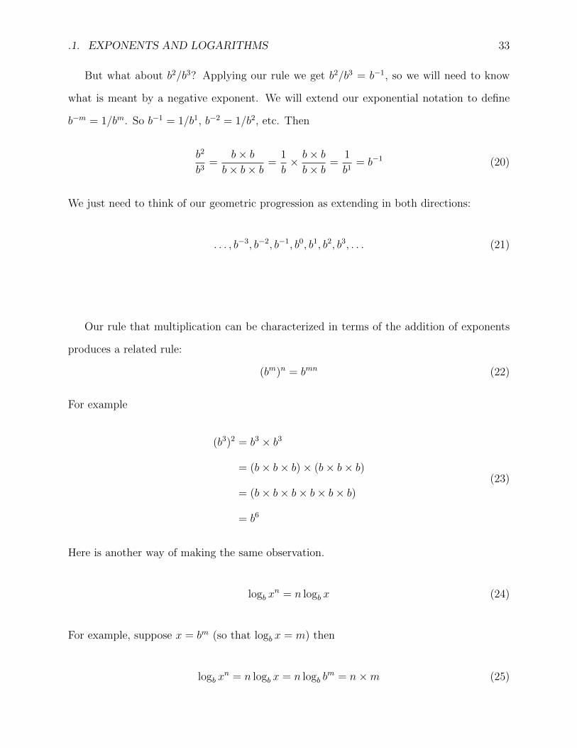
But what about b2/b3? Applying our rule we get b2/b3 = b−1, so we will need to know
what is meant by a negative exponent. We will extend our exponential notation to define
b−m = 1/bm. So b−1 = 1/b1, b−2 = 1/b2, etc. Then
b2
b3=
b× bb× b× b =
1
b× b× bb× b =
1
b1= b−1 (20)
We just need to think of our geometric progression as extending in both directions:
. . . , b−3, b−2, b−1, b0, b1, b2, b3, . . . (21)
Our rule that multiplication can be characterized in terms of the addition of exponents
produces a related rule:
(bm)n = bmn (22)
For example
(b3)2 = b3 × b3
= (b× b× b)× (b× b× b)
= (b× b× b× b× b× b)
= b6
(23)
Here is another way of making the same observation.
logb xn = n logb x (24)
For example, suppose x = bm (so that logb x = m) then
logb xn = n logb x = n logb b
m = n×m (25)
34 BIBLIOGRAPHY
In summary, we have developed three useful rules in our discussion of logarithms.
logb(xy) = logb x+ logb y (26)
logb(x/y) = logb x− logb y (27)
logb xk = k logb x (28)
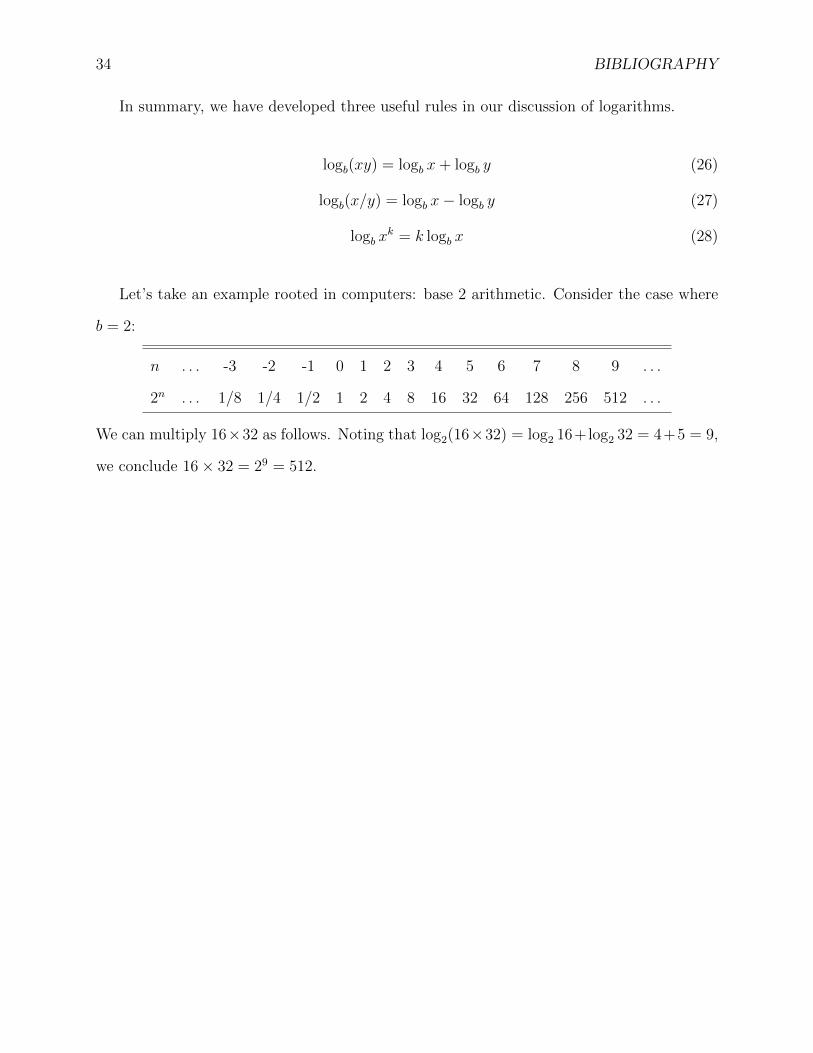
Let’s take an example rooted in computers: base 2 arithmetic. Consider the case where
b = 2:
n . . . -3 -2 -1 0 1 2 3 4 5 6 7 8 9 . . .
2n . . . 1/8 1/4 1/2 1 2 4 8 16 32 64 128 256 512 . . .
We can multiply 16×32 as follows. Noting that log2(16×32) = log2 16+log2 32 = 4+5 = 9,
we conclude 16× 32 = 29 = 512.
.2. EXPECTATIONS, CONSISTENCY, AND EFFICIENCY 35
.2 Expectations, Consistency, and Efficiency
By now it should be clear that we cannot go very far in our thinking about financial mar-
kets without thinking about expectations. Economists consider this a major problem, since
expectations cannot be observed. Rather than simply treat expectations as an unobserved
exogenous influence on financial markets, economists impose certain structure upon expec-
tations. Two common structures are the expectations be self-consistent and informationally
efficient.
.2.1 Law of Iterated Expectations
Linearity
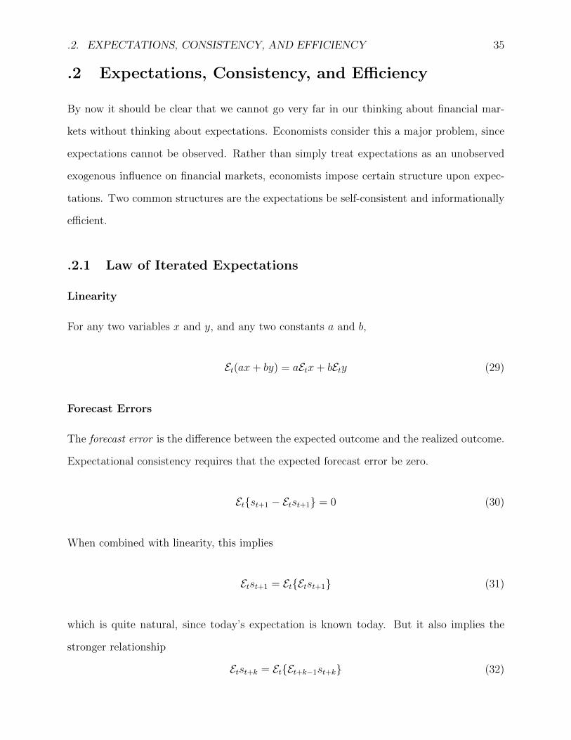
For any two variables x and y, and any two constants a and b,
Et(ax+ by) = aEtx+ bEty (29)
Forecast Errors
The forecast error is the difference between the expected outcome and the realized outcome.
Expectational consistency requires that the expected forecast error be zero.
Et{st+1 − Etst+1} = 0 (30)
When combined with linearity, this implies
Etst+1 = Et{Etst+1} (31)
which is quite natural, since today’s expectation is known today. But it also implies the
stronger relationship
Etst+k = Et{Et+k−1st+k} (32)
36 BIBLIOGRAPHY
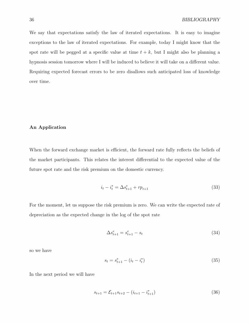
We say that expectations satisfy the law of iterated expectations. It is easy to imagine
exceptions to the law of iterated expectations. For example, today I might know that the
spot rate will be pegged at a specific value at time t + k, but I might also be planning a
hypnosis session tomorrow where I will be induced to believe it will take on a different value.
Requiring expected forecast errors to be zero disallows such anticipated loss of knowledge
over time.
An Application
When the forward exchange market is efficient, the forward rate fully reflects the beliefs of
the market participants. This relates the interest differential to the expected value of the
future spot rate and the risk premium on the domestic currency.
it − i∗t = ∆set+1 + rpt+1 (33)
For the moment, let us suppose the risk premium is zero. We can write the expected rate of
depreciation as the expected change in the log of the spot rate
∆set+1 = set+1 − st (34)
so we have
st = set+1 − (it − i∗t ) (35)
In the next period we will have
st+1 = Et+1st+2 − (it+1 − i∗t+1) (36)
.2. EXPECTATIONS, CONSISTENCY, AND EFFICIENCY 37
Applying the law of iterated expectations, we know that our expectation today of our next
period’s expectation is just our expectation today of the two period ahead spot rate.
EtEt+1st+2 = Etst+2 (37)
Secondly, individuals should expect that (35) will hold in the future.
st+1 = Et+1st+2 − (it+1 − i∗t+1) (38)
Together these give us
Etst+1 = Etst+2 − Et(it+1 − i∗t+1) (39)
Etst+2 = Etst+3 − Et(it+2 − i∗t+2) (40)
... (41)
Applying these relationships repeatedly to (35), we get
s = Etst+1 − (it − i∗t )
= Etst+2 −∑k=0
1(it+ − i∗t+k)
= limT→∞{Etst+T+1 −
T∑k=0
(it+ − i∗t+k)}
(42)
Informational Efficiency
Economists have meant a number of different things by the efficient markets hypothesis.
Most often, the hypothesis is that markets are not only efficient, but are also informationally
efficient. That is, not only do market prices fully reflect the beliefs of market participants,
but the beliefs of market participants fully reflect the available information. When this is
the case, economists like to say that expectations are “rational”. What they mean is that

38 BIBLIOGRAPHY
market participants do not make systematic (i.e., predictable) forecasting errors.
Let the information available at time t be It. Let E{·|It} denote the mathematical
expectation conditional on this information. Then expectations are “rational” if
∆set+1 = E{∆st+1|It} (43)
When there is no danger of ambiguity about the information set, we will just write
∆set+1 = Et∆st+1 (44)
Following Fama (1970), we can distinguish various degrees of market efficiency. A market
is informationally efficient relative to It if “abnormal returns” cannot be obtained using only
the information in It. A market that is efficient relative to the past history of prices is called
weakly efficient. A market that is efficient relative to all publically available information
is called semi-strong form efficient. A market that is efficient relative to all publically and
privately available information is called strong form efficient.
Consider the forecast error
εt+1 = ∆s− E{∆st+1|It} (45)
Note that the expected value of the forecast error, given information It, is zero.