Embed Size (px)
Citation preview
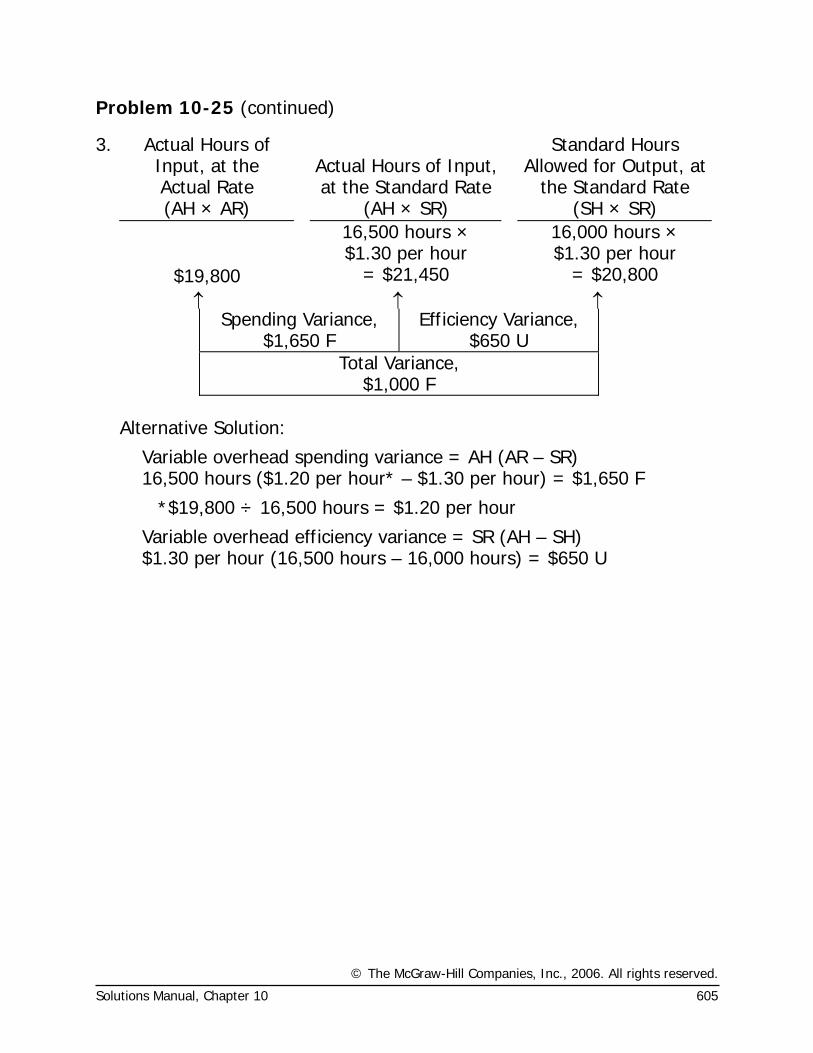
© The McGraw-Hill Companies, Inc., 2006. All rights reserved.
Solutions Manual, Chapter 10 545
Chapter 10 Standard Costs and the Balanced Scorecard
Solutions to Questions
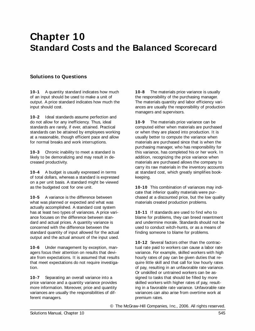
10-1 A quantity standard indicates how much of an input should be used to make a unit of output. A price standard indicates how much the input should cost.
10-2 Ideal standards assume perfection and do not allow for any inefficiency. Thus, ideal standards are rarely, if ever, attained. Practical standards can be attained by employees working at a reasonable, though efficient pace and allow for normal breaks and work interruptions.
10-3 Chronic inability to meet a standard is likely to be demoralizing and may result in de-creased productivity.
10-4 A budget is usually expressed in terms of total dollars, whereas a standard is expressed on a per unit basis. A standard might be viewed as the budgeted cost for one unit.
10-5 A variance is the difference between what was planned or expected and what was actually accomplished. A standard cost system has at least two types of variances. A price vari-ance focuses on the difference between stan-dard and actual prices. A quantity variance is concerned with the difference between the standard quantity of input allowed for the actual output and the actual amount of the input used.
10-6 Under management by exception, man-agers focus their attention on results that devi-ate from expectations. It is assumed that results that meet expectations do not require investiga-tion.
10-7 Separating an overall variance into a price variance and a quantity variance provides more information. Moreover, price and quantity variances are usually the responsibilities of dif-ferent managers.
10-8 The materials price variance is usually the responsibility of the purchasing manager. The materials quantity and labor efficiency vari-ances are usually the responsibility of production managers and supervisors.
10-9 The materials price variance can be computed either when materials are purchased or when they are placed into production. It is usually better to compute the variance when materials are purchased since that is when the purchasing manager, who has responsibility for this variance, has completed his or her work. In addition, recognizing the price variance when materials are purchased allows the company to carry its raw materials in the inventory accounts at standard cost, which greatly simplifies book-keeping.
10-10 This combination of variances may indi-cate that inferior quality materials were pur-chased at a discounted price, but the low quality materials created production problems.
10-11 If standards are used to find who to blame for problems, they can breed resentment and undermine morale. Standards should not be used to conduct witch-hunts, or as a means of finding someone to blame for problems.
10-12 Several factors other than the contrac-tual rate paid to workers can cause a labor rate variance. For example, skilled workers with high hourly rates of pay can be given duties that re-quire little skill and that call for low hourly rates of pay, resulting in an unfavorable rate variance. Or unskilled or untrained workers can be as-signed to tasks that should be filled by more skilled workers with higher rates of pay, result-ing in a favorable rate variance. Unfavorable rate variances can also arise from overtime work at premium rates.
© The McGraw-Hill Companies, Inc., 2006. All rights reserved.
546 Managerial Accounting, 11th Edition
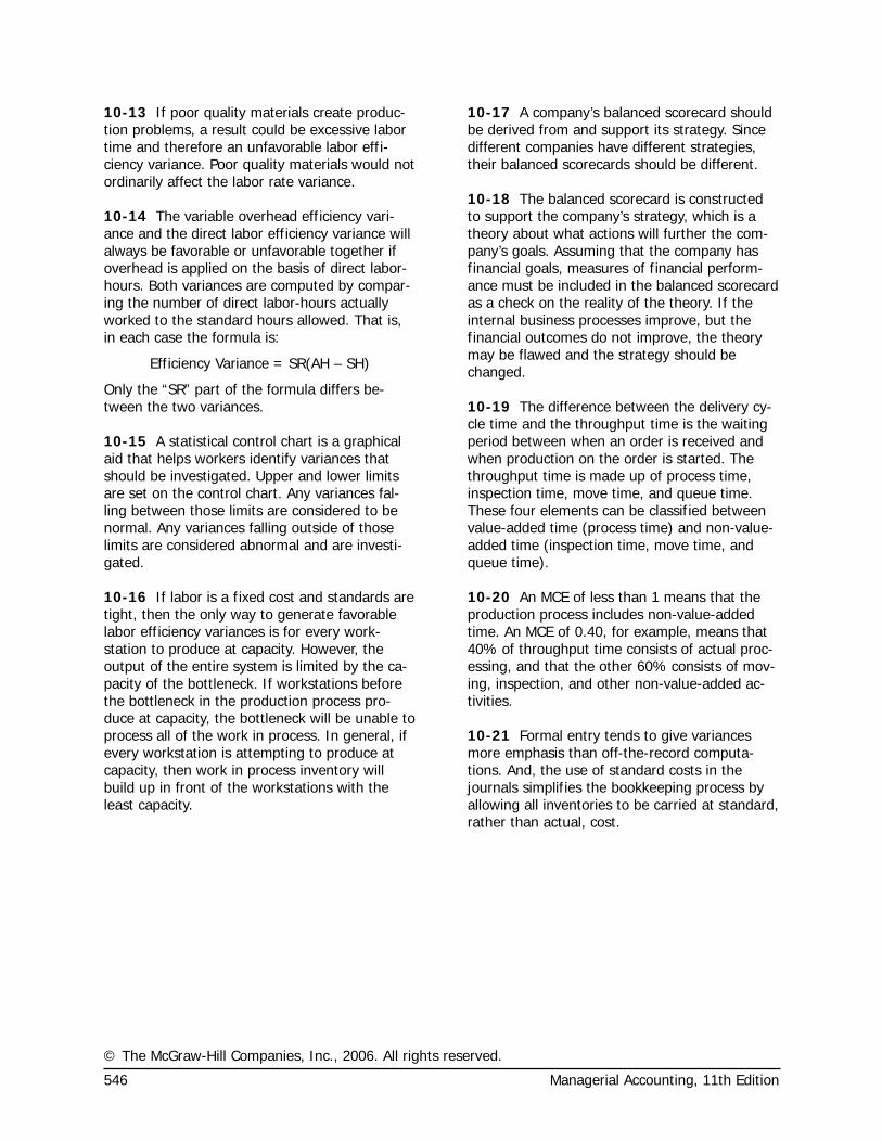
10-13 If poor quality materials create produc-tion problems, a result could be excessive labor time and therefore an unfavorable labor effi-ciency variance. Poor quality materials would not ordinarily affect the labor rate variance.
10-14 The variable overhead efficiency vari-ance and the direct labor efficiency variance will always be favorable or unfavorable together if overhead is applied on the basis of direct labor-hours. Both variances are computed by compar-ing the number of direct labor-hours actually worked to the standard hours allowed. That is, in each case the formula is:
Efficiency Variance = SR(AH – SH)
Only the “SR” part of the formula differs be-tween the two variances.
10-15 A statistical control chart is a graphical aid that helps workers identify variances that should be investigated. Upper and lower limits are set on the control chart. Any variances fal-ling between those limits are considered to be normal. Any variances falling outside of those limits are considered abnormal and are investi-gated.
10-16 If labor is a fixed cost and standards are tight, then the only way to generate favorable labor efficiency variances is for every work-station to produce at capacity. However, the output of the entire system is limited by the ca-pacity of the bottleneck. If workstations before the bottleneck in the production process pro-duce at capacity, the bottleneck will be unable to process all of the work in process. In general, if every workstation is attempting to produce at capacity, then work in process inventory will build up in front of the workstations with the least capacity.
10-17 A company’s balanced scorecard should be derived from and support its strategy. Since different companies have different strategies, their balanced scorecards should be different.
10-18 The balanced scorecard is constructed to support the company’s strategy, which is a theory about what actions will further the com-pany’s goals. Assuming that the company has financial goals, measures of financial perform-ance must be included in the balanced scorecard as a check on the reality of the theory. If the internal business processes improve, but the financial outcomes do not improve, the theory may be flawed and the strategy should be changed.
10-19 The difference between the delivery cy-cle time and the throughput time is the waiting period between when an order is received and when production on the order is started. The throughput time is made up of process time, inspection time, move time, and queue time. These four elements can be classified between value-added time (process time) and non-value-added time (inspection time, move time, and queue time).
10-20 An MCE of less than 1 means that the production process includes non-value-added time. An MCE of 0.40, for example, means that 40% of throughput time consists of actual proc-essing, and that the other 60% consists of mov-ing, inspection, and other non-value-added ac-tivities.
10-21 Formal entry tends to give variances more emphasis than off-the-record computa-tions. And, the use of standard costs in the journals simplifies the bookkeeping process by allowing all inventories to be carried at standard, rather than actual, cost.
© The McGraw-Hill Companies, Inc., 2006. All rights reserved.
Solutions Manual, Chapter 10 547
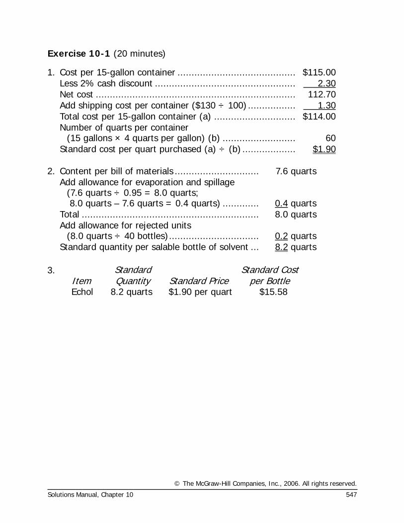
Exercise 10-1 (20 minutes)
1. Cost per 15-gallon container .......................................... $115.00 Less 2% cash discount .................................................. 2.30 Net cost ....................................................................... 112.70 Add shipping cost per container ($130 ÷ 100) ................. 1.30 Total cost per 15-gallon container (a) ............................. $114.00
Number of quarts per container
(15 gallons × 4 quarts per gallon) (b) .......................... 60 Standard cost per quart purchased (a) ÷ (b) ................... $1.90 2. Content per bill of materials .............................. 7.6 quarts
Add allowance for evaporation and spillage (7.6 quarts ÷ 0.95 = 8.0 quarts; 8.0 quarts – 7.6 quarts = 0.4 quarts) ............. 0.4 quarts
Total ............................................................... 8.0 quarts
Add allowance for rejected units
(8.0 quarts ÷ 40 bottles)................................ 0.2 quarts Standard quantity per salable bottle of solvent ... 8.2 quarts 3.
Item
Standard Quantity Standard Price
Standard Cost per Bottle
Echol 8.2 quarts $1.90 per quart $15.58
© The McGraw-Hill Companies, Inc., 2006. All rights reserved.
548 Managerial Accounting, 11th Edition
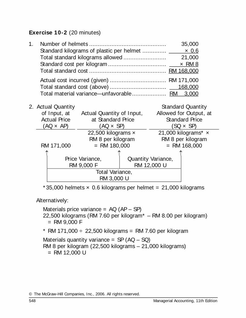
Exercise 10-2 (20 minutes)
1. Number of helmets ............................................. 35,000 Standard kilograms of plastic per helmet .............. × 0.6 Total standard kilograms allowed ......................... 21,000 Standard cost per kilogram.................................. × RM 8 Total standard cost ............................................. RM 168,000
Actual cost incurred (given) ................................. RM 171,000 Total standard cost (above) ................................. 168,000 Total material variance—unfavorable .................... RM 3,000 2. Actual Quantity
of Input, at Actual Price
Actual Quantity of Input,
at Standard Price
Standard Quantity Allowed for Output, at
Standard Price (AQ × AP) (AQ × SP) (SQ × SP) 22,500 kilograms × 21,000 kilograms* × RM 8 per kilogram RM 8 per kilogram RM 171,000 = RM 180,000 = RM 168,000 ↑ ↑ ↑
Price Variance, RM 9,000 F
Quantity Variance, RM 12,000 U
Total Variance, RM 3,000 U
*35,000 helmets × 0.6 kilograms per helmet = 21,000 kilograms Alternatively:
Materials price variance = AQ (AP – SP) 22,500 kilograms (RM 7.60 per kilogram* – RM 8.00 per kilogram) = RM 9,000 F
* RM 171,000 ÷ 22,500 kilograms = RM 7.60 per kilogram
Materials quantity variance = SP (AQ – SQ) RM 8 per kilogram (22,500 kilograms – 21,000 kilograms) = RM 12,000 U
© The McGraw-Hill Companies, Inc., 2006. All rights reserved.
Solutions Manual, Chapter 10 549
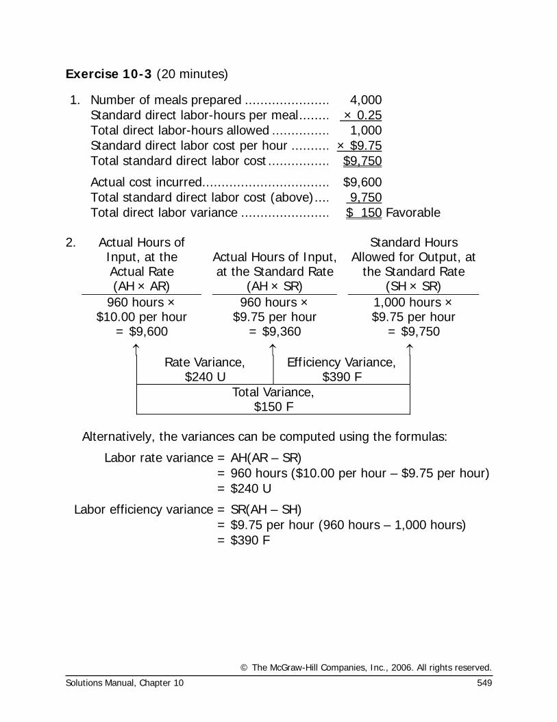
Exercise 10-3 (20 minutes)
1. Number of meals prepared ...................... 4,000 Standard direct labor-hours per meal........ × 0.25 Total direct labor-hours allowed ............... 1,000 Standard direct labor cost per hour .......... × $9.75 Total standard direct labor cost ................ $9,750
Actual cost incurred................................. $9,600 Total standard direct labor cost (above).... 9,750 Total direct labor variance ....................... $ 150 Favorable
2. Actual Hours of
Input, at the Actual Rate
Actual Hours of Input, at the Standard Rate
Standard Hours Allowed for Output, at
the Standard Rate (AH × AR) (AH × SR) (SH × SR) 960 hours ×
$10.00 per hour 960 hours ×
$9.75 per hour 1,000 hours × $9.75 per hour
= $9,600 = $9,360 = $9,750 ↑ ↑ ↑
Rate Variance, $240 U
Efficiency Variance, $390 F
Total Variance, $150 F
Alternatively, the variances can be computed using the formulas:
Labor rate variance = AH(AR – SR) = 960 hours ($10.00 per hour – $9.75 per hour) = $240 U
Labor efficiency variance = SR(AH – SH) = $9.75 per hour (960 hours – 1,000 hours) = $390 F
© The McGraw-Hill Companies, Inc., 2006. All rights reserved.
550 Managerial Accounting, 11th Edition
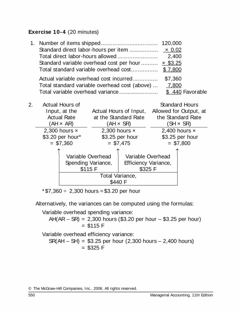
Exercise 10-4 (20 minutes)
1. Number of items shipped.................................. 120,000 Standard direct labor-hours per item ................. × 0.02 Total direct labor-hours allowed ........................ 2,400 Standard variable overhead cost per hour .......... × $3.25 Total standard variable overhead cost................ $ 7,800
Actual variable overhead cost incurred............... $7,360 Total standard variable overhead cost (above) ... 7,800 Total variable overhead variance ....................... $ 440 Favorable
2. Actual Hours of
Input, at the Actual Rate
Actual Hours of Input, at the Standard Rate
Standard Hours Allowed for Output, at
the Standard Rate (AH × AR) (AH × SR) (SH × SR) 2,300 hours ×
$3.20 per hour* 2,300 hours ×
$3.25 per hour 2,400 hours × $3.25 per hour
= $7,360 = $7,475 = $7,800 ↑ ↑ ↑
Variable Overhead Spending Variance,
$115 F
Variable Overhead Efficiency Variance,
$325 F Total Variance,
$440 F
*$7,360 ÷ 2,300 hours =$3.20 per hour Alternatively, the variances can be computed using the formulas:
Variable overhead spending variance: AH(AR – SR) = 2,300 hours ($3.20 per hour – $3.25 per hour) = $115 F
Variable overhead efficiency variance: SR(AH – SH) = $3.25 per hour (2,300 hours – 2,400 hours) = $325 F
© The McGraw-Hill Companies, Inc., 2006. All rights reserved.
Solutions Manual, Chapter 10 551
Exercise 10-5 (45 minutes)
1. MPC’s previous manufacturing strategy was focused on high-volume production of a limited range of paper grades. The goal of this strategy was to keep the machines running constantly to maximize the number of tons produced. Changeovers were avoided because they lowered equipment utilization. Maximizing tons produced and minimizing changeovers helped spread the high fixed costs of paper manufacturing across more units of output. The new manufacturing strategy is focused on low-volume production of a wide range of products. The goals of this strategy are to increase the number of paper grades manufactured, de-crease changeover times, and increase yields across non-standard grades. While MPC realizes that its new strategy will decrease its equip-ment utilization, it will still strive to optimize the utilization of its high fixed cost resources within the confines of flexible production. In an economist’s terms the old strategy focused on economies of scale while the new strategy focuses on economies of scope.
2. Employees focus on improving those measures that are used to evaluate
their performance. Therefore, strategically-aligned performance meas-ures will channel employee effort towards improving those aspects of performance that are most important to obtaining strategic objectives. If a company changes its strategy but continues to evaluate employee per-formance using measures that do not support the new strategy, it will be motivating its employees to make decisions that promote the old strategy, not the new strategy. And if employees make decisions that promote the new strategy, their performance measures will suffer.
Some performance measures that would be appropriate for MPC’s old
strategy include: equipment utilization percentage, number of tons of paper produced, and cost per ton produced. These performance meas-ures would not support MPC’s new strategy because they would dis-courage increasing the range of paper grades produced, increasing the number of changeovers performed, and decreasing the batch size pro-duced per run.
© The McGraw-Hill Companies, Inc., 2006. All rights reserved.
552 Managerial Accounting, 11th Edition
Exercise 10-5 (continued)
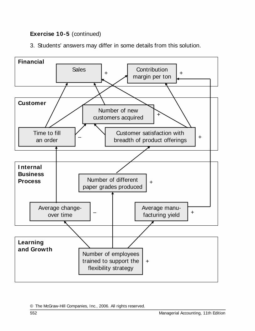
3. Students’ answers may differ in some details from this solution.
Sales Contribution margin per ton
Financial
Time to fill an order
Customer satisfaction with breadth of product offerings
Number of new customers acquired
Customer
Average change-over time
Number of different paper grades produced
Average manu-facturing yield
Internal Business Process
Number of employees trained to support the
flexibility strategy
Learning and Growth
+
– +
+
– +
+
+ +
© The McGraw-Hill Companies, Inc., 2006. All rights reserved.
Solutions Manual, Chapter 10 553
Exercise 10-5 (continued)
4. The hypotheses underlying the balanced scorecard are indicated by the arrows in the diagram. Reading from the bottom of the balanced score-card, the hypotheses are:
° If the number of employees trained to support the flexibility strategy increases, then the average changeover time will decrease and the number of different paper grades produced and the average manu-facturing yield will increase.
° If the average change-over time decreases, then the time to fill an order will decrease.
° If the number of different paper grades produced increases, then the customer satisfaction with breadth of product offerings will increase.
° If the average manufacturing yield increases, then the contribution margin per ton will increase.
° If the time to fill an order decreases, then the number of new cus-tomers acquired, sales, and the contribution margin per ton will in-crease.
° If the customer satisfaction with breadth of product offerings in-creases, then the number of new customers acquired, sales, and the contribution margin per ton will increase.
° If the number of new customers acquired increases, then sales will increase.
Each of these hypotheses is questionable to some degree. For example,
the time to fill an order is a function of additional factors above and be-yond changeover times. Thus, MPC’s average changeover time could decrease while its time to fill an order increases if, for example, the shipping department proves to be incapable of efficiently handling greater product diversity, smaller batch sizes, and more frequent ship-ments. The fact that each of the hypotheses mentioned above can be questioned does not invalidate the balanced scorecard. If the scorecard is used correctly, management will be able to identify which, if any, of the hypotheses are invalid and modify the balanced scorecard accord-ingly.
© The McGraw-Hill Companies, Inc., 2006. All rights reserved.
554 Managerial Accounting, 11th Edition
Exercise 10-6 (20 minutes)
1.
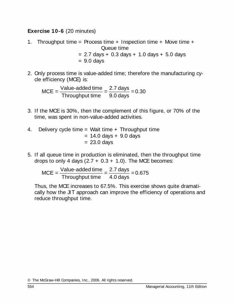
Throughput time = Process time + Inspection time + Move time + Queue time
= 2.7 days + 0.3 days + 1.0 days + 5.0 days = 9.0 days 2. Only process time is value-added time; therefore the manufacturing cy-
cle efficiency (MCE) is:
-Value added time 2.7 daysMCE = = = 0.30
Throughput time 9.0 days
3. If the MCE is 30%, then the complement of this figure, or 70% of the
time, was spent in non-value-added activities. 4. Delivery cycle time = Wait time + Throughput time = 14.0 days + 9.0 days = 23.0 days 5. If all queue time in production is eliminated, then the throughput time
drops to only 4 days (2.7 + 0.3 + 1.0). The MCE becomes:
-Value added time 2.7 daysMCE = = = 0.675
Throughput time 4.0 days
Thus, the MCE increases to 67.5%. This exercise shows quite dramati-cally how the JIT approach can improve the efficiency of operations and reduce throughput time.
© The McGraw-Hill Companies, Inc., 2006. All rights reserved.
Solutions Manual, Chapter 10 555
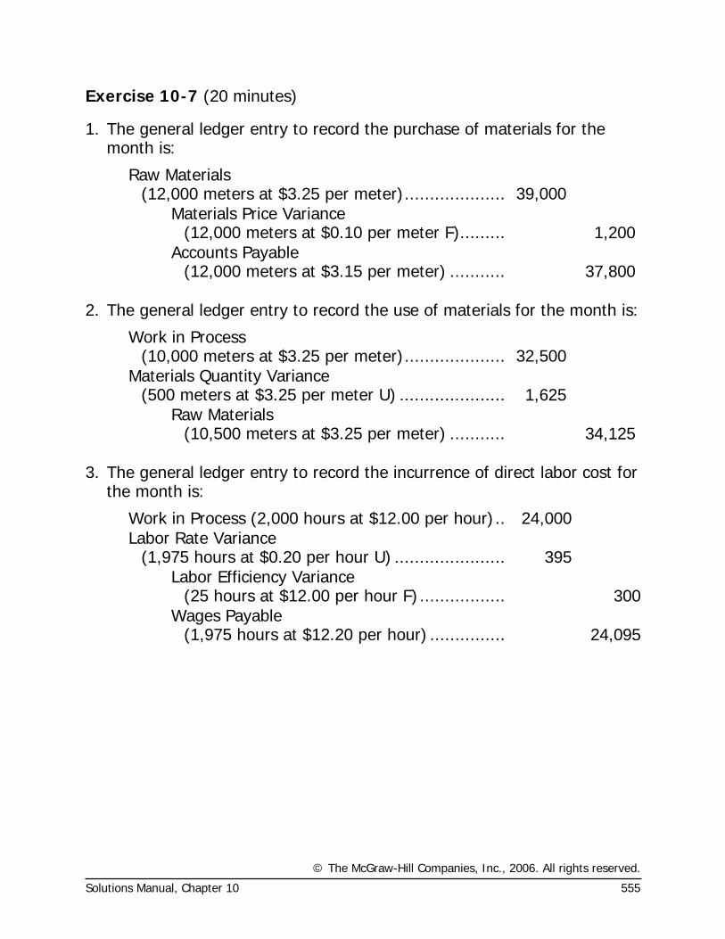
Exercise 10-7 (20 minutes)
1. The general ledger entry to record the purchase of materials for the month is:
Raw Materials
(12,000 meters at $3.25 per meter)..................... 39,000
Materials Price Variance
(12,000 meters at $0.10 per meter F).......... 1,200
Accounts Payable
(12,000 meters at $3.15 per meter) ............ 37,800 2. The general ledger entry to record the use of materials for the month is:
Work in Process
(10,000 meters at $3.25 per meter)..................... 32,500
Materials Quantity Variance
(500 meters at $3.25 per meter U) ...................... 1,625
Raw Materials
(10,500 meters at $3.25 per meter) ............ 34,125 3. The general ledger entry to record the incurrence of direct labor cost for
the month is:
Work in Process (2,000 hours at $12.00 per hour)... 24,000
Labor Rate Variance
(1,975 hours at $0.20 per hour U) ....................... 395
Labor Efficiency Variance
(25 hours at $12.00 per hour F).................. 300
Wages Payable
(1,975 hours at $12.20 per hour) ................ 24,095

© The McGraw-Hill Companies, Inc., 2006. All rights reserved.
556 Managerial Accounting, 11th Edition
Exercise 10-8 (20 minutes)
1. The standard price of a kilogram of white chocolate is determined as fol-lows:
Purchase price, finest grade white chocolate ........................ £7.50 Less purchase discount, 8% of the purchase price of £7.50 ... (0.60) Shipping cost from the supplier in Belgium........................... 0.30 Receiving and handling cost................................................ 0.04 Standard price per kilogram of white chocolate..................... £7.24
2. The standard quantity, in kilograms, of white chocolate in a dozen truf-
fles is computed as follows:
Material requirements............................... 0.70 Allowance for waste ................................. 0.03 Allowance for rejects ................................ 0.02 Standard quantity of white chocolate ......... 0.75
3. The standard cost of the white chocolate in a dozen truffles is deter-
mined as follows:
Standard quantity of white chocolate (a)....... 0.75 kilogram Standard price of white chocolate (b) ........... £7.24 per kilogram Standard cost of white chocolate (a) × (b).... £5.43
© The McGraw-Hill Companies, Inc., 2006. All rights reserved.
Solutions Manual, Chapter 10 557
Exercise 10-9 (30 minutes)
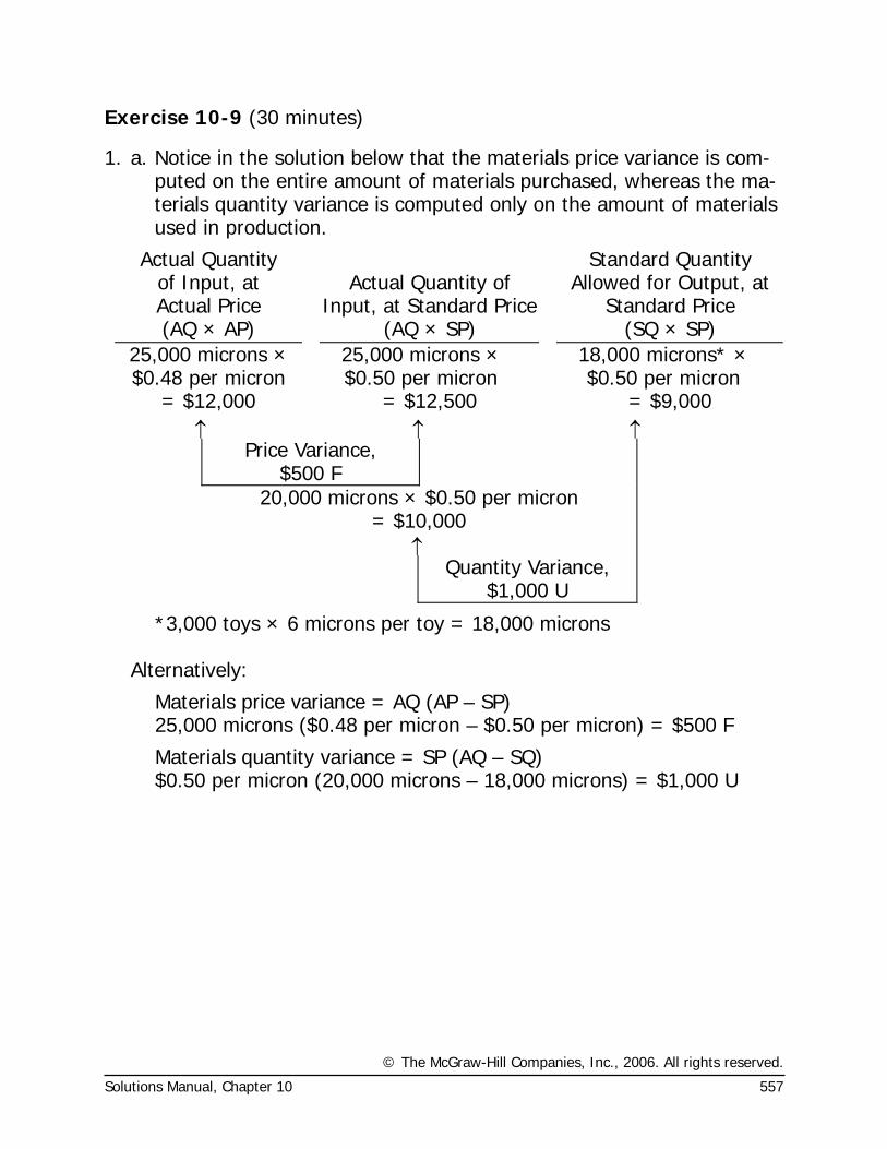
1. a. Notice in the solution below that the materials price variance is com-puted on the entire amount of materials purchased, whereas the ma-terials quantity variance is computed only on the amount of materials used in production.
Actual Quantity of Input, at Actual Price
Actual Quantity of
Input, at Standard Price
Standard Quantity Allowed for Output, at
Standard Price (AQ × AP) (AQ × SP) (SQ × SP)
25,000 microns × $0.48 per micron
25,000 microns × $0.50 per micron
18,000 microns* × $0.50 per micron
= $12,000 = $12,500 = $9,000 ↑ ↑ ↑
Price Variance, $500 F
20,000 microns × $0.50 per micron = $10,000
↑ Quantity Variance,
$1,000 U
*3,000 toys × 6 microns per toy = 18,000 microns Alternatively:
Materials price variance = AQ (AP – SP) 25,000 microns ($0.48 per micron – $0.50 per micron) = $500 F
Materials quantity variance = SP (AQ – SQ) $0.50 per micron (20,000 microns – 18,000 microns) = $1,000 U
© The McGraw-Hill Companies, Inc., 2006. All rights reserved.
558 Managerial Accounting, 11th Edition
Exercise 10-9 (continued)
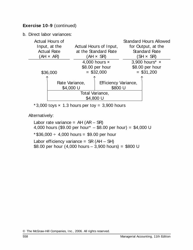
b. Direct labor variances:
Actual Hours of Input, at the Actual Rate
Actual Hours of Input, at the Standard Rate
Standard Hours Allowed for Output, at the
Standard Rate (AH × AR) (AH × SR) (SH × SR)
4,000 hours × $8.00 per hour
3,900 hours* × $8.00 per hour
$36,000 = $32,000 = $31,200 ↑ ↑ ↑
Rate Variance, $4,000 U
Efficiency Variance, $800 U
Total Variance, $4,800 U
*3,000 toys × 1.3 hours per toy = 3,900 hours Alternatively:
Labor rate variance = AH (AR – SR) 4,000 hours ($9.00 per hour* – $8.00 per hour) = $4,000 U
*$36,000 ÷ 4,000 hours = $9.00 per hour
Labor efficiency variance = SR (AH – SH) $8.00 per hour (4,000 hours – 3,900 hours) = $800 U
© The McGraw-Hill Companies, Inc., 2006. All rights reserved.
Solutions Manual, Chapter 10 559
Exercise 10-9 (continued)
2. A variance usually has many possible explanations. In particular, we should always keep in mind that the standards themselves may be in-correct. Some of the other possible explanations for the variances ob-served at Dawson Toys appear below:
Materials Price Variance Since this variance is favorable, the actual price paid per unit for the material was less than the standard price. This could occur for a variety of reasons including the purchase of a lower grade ma-terial at a discount, buying in an unusually large quantity to take advan-tage of quantity discounts, a change in the market price of the material, or particularly sharp bargaining by the purchasing department.
Materials Quantity Variance Since this variance is unfavorable, more ma-terials were used to produce the actual output than were called for by the standard. This could also occur for a variety of reasons. Some of the pos-sibilities include poorly trained or supervised workers, improperly adjusted machines, and defective materials.
Labor Rate Variance Since this variance is unfavorable, the actual aver-age wage rate was higher than the standard wage rate. Some of the pos-sible explanations include an increase in wages that has not been re-flected in the standards, unanticipated overtime, and a shift toward more highly paid workers.
Labor Efficiency Variance Since this variance is unfavorable, the actual number of labor hours was greater than the standard labor hours allowed for the actual output. As with the other variances, this variance could have been caused by any of a number of factors. Some of the possible explana-tions include poor supervision, poorly trained workers, low quality materi-als requiring more labor time to process, and machine breakdowns. In addition, if the direct labor force is essentially fixed, an unfavorable labor efficiency variance could be caused by a reduction in output due to de-creased demand for the company’s products.
It is worth noting that all of these variances could have been caused by the purchase of low quality materials at a cut-rate price.
© The McGraw-Hill Companies, Inc., 2006. All rights reserved.
560 Managerial Accounting, 11th Edition
Exercise 10-10 (20 minutes)
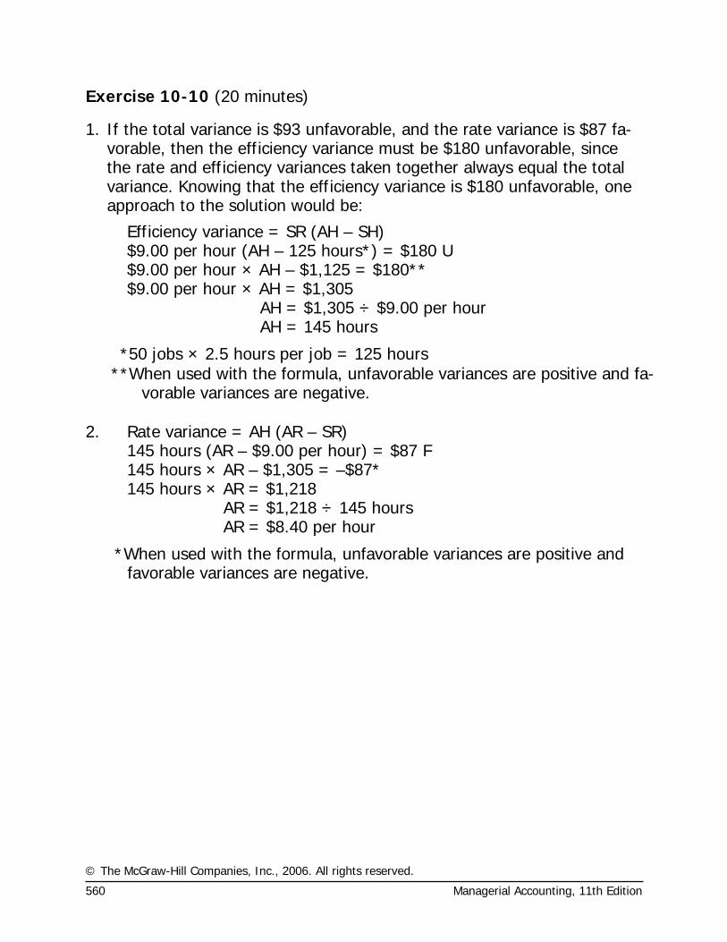
1. If the total variance is $93 unfavorable, and the rate variance is $87 fa-vorable, then the efficiency variance must be $180 unfavorable, since the rate and efficiency variances taken together always equal the total variance. Knowing that the efficiency variance is $180 unfavorable, one approach to the solution would be:
Efficiency variance = SR (AH – SH) $9.00 per hour (AH – 125 hours*) = $180 U $9.00 per hour × AH – $1,125 = $180** $9.00 per hour × AH = $1,305 AH = $1,305 ÷ $9.00 per hour AH = 145 hours
*50 jobs × 2.5 hours per job = 125 hours **When used with the formula, unfavorable variances are positive and fa-
vorable variances are negative. 2. Rate variance = AH (AR – SR) 145 hours (AR – $9.00 per hour) = $87 F 145 hours × AR – $1,305 = –$87* 145 hours × AR = $1,218 AR = $1,218 ÷ 145 hours AR = $8.40 per hour
*When used with the formula, unfavorable variances are positive and
favorable variances are negative.
© The McGraw-Hill Companies, Inc., 2006. All rights reserved.
Solutions Manual, Chapter 10 561
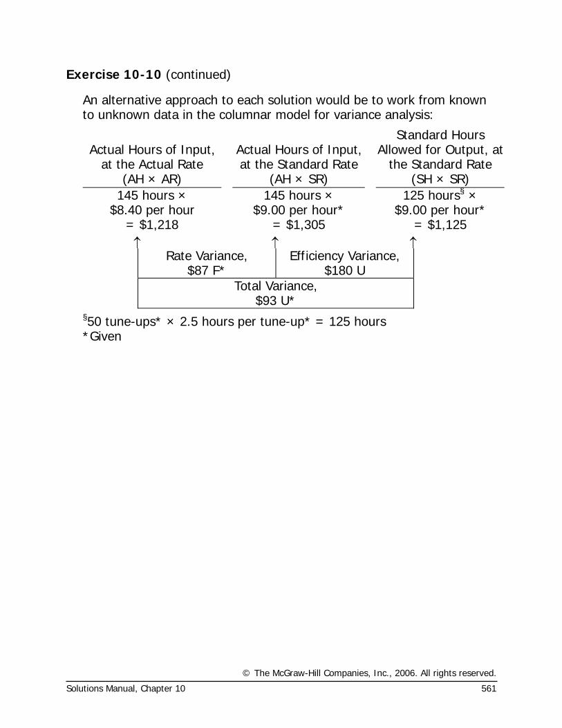
Exercise 10-10 (continued)
An alternative approach to each solution would be to work from known to unknown data in the columnar model for variance analysis:
Actual Hours of Input,
at the Actual Rate
Actual Hours of Input, at the Standard Rate
Standard Hours Allowed for Output, at
the Standard Rate (AH × AR) (AH × SR) (SH × SR)
145 hours × $8.40 per hour
145 hours × $9.00 per hour*
125 hours§ × $9.00 per hour*
= $1,218 = $1,305 = $1,125 ↑ ↑ ↑
Rate Variance, $87 F*
Efficiency Variance, $180 U
Total Variance, $93 U*
§50 tune-ups* × 2.5 hours per tune-up* = 125 hours *Given
© The McGraw-Hill Companies, Inc., 2006. All rights reserved.
562 Managerial Accounting, 11th Edition
Exercise 10-11 (30 minutes)
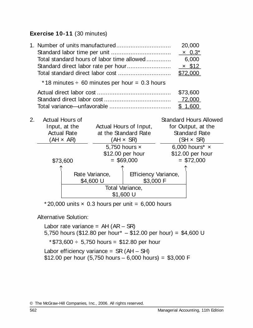
1. Number of units manufactured............................... 20,000 Standard labor time per unit .................................. × 0.3* Total standard hours of labor time allowed .............. 6,000 Standard direct labor rate per hour......................... × $12 Total standard direct labor cost .............................. $72,000
*18 minutes ÷ 60 minutes per hour = 0.3 hours
Actual direct labor cost .......................................... $73,600 Standard direct labor cost ...................................... 72,000 Total variance—unfavorable ................................... $ 1,600 2. Actual Hours of
Input, at the Actual Rate
Actual Hours of Input, at the Standard Rate
Standard Hours Allowed for Output, at the
Standard Rate (AH × AR) (AH × SR) (SH × SR) 5,750 hours ×
$12.00 per hour 6,000 hours* ×
$12.00 per hour $73,600 = $69,000 = $72,000 ↑ ↑ ↑
Rate Variance, $4,600 U
Efficiency Variance, $3,000 F
Total Variance, $1,600 U
*20,000 units × 0.3 hours per unit = 6,000 hours Alternative Solution:
Labor rate variance = AH (AR – SR) 5,750 hours ($12.80 per hour* – $12.00 per hour) = $4,600 U
*$73,600 ÷ 5,750 hours = $12.80 per hour
Labor efficiency variance = SR (AH – SH) $12.00 per hour (5,750 hours – 6,000 hours) = $3,000 F

© The McGraw-Hill Companies, Inc., 2006. All rights reserved.
Solutions Manual, Chapter 10 563
Exercise 10-11 (continued)
3. Actual Hours of Input, at the Actual Rate
Actual Hours of Input, at the Standard Rate
Standard Hours Allowed for Output, at
the Standard Rate (AH × AR) (AH × SR) (SH × SR) 5,750 hours ×
$4.00 per hour 6,000 hours ×
$4.00 per hour $21,850 = $23,000 = $24,000 ↑ ↑ ↑
Spending Variance, $1,150 F
Efficiency Variance, $1,000 F
Total Variance, $2,150 F
Alternative Solution:
Variable overhead spending variance = AH (AR – SR) 5,750 hours ($3.80 per hour* – $4.00 per hour) = $1,150 F
*$21,850 ÷ 5,750 hours = $3.80 per hour
Variable overhead efficiency variance = SR (AH – SH) $4.00 per hour (5,750 hours – 6,000 hours) = $1,000 F
© The McGraw-Hill Companies, Inc., 2006. All rights reserved.
564 Managerial Accounting, 11th Edition
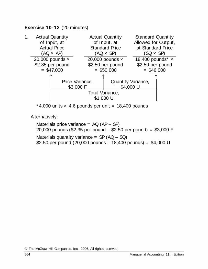
Exercise 10-12 (20 minutes)
1. Actual Quantity of Input, at Actual Price
Actual Quantity of Input, at
Standard Price
Standard Quantity Allowed for Output, at Standard Price
(AQ × AP) (AQ × SP) (SQ × SP) 20,000 pounds ×
$2.35 per pound 20,000 pounds ×
$2.50 per pound 18,400 pounds* ×
$2.50 per pound = $47,000 = $50,000 = $46,000 ↑ ↑ ↑
Price Variance, $3,000 F
Quantity Variance, $4,000 U
Total Variance, $1,000 U
*4,000 units × 4.6 pounds per unit = 18,400 pounds Alternatively:
Materials price variance = AQ (AP – SP) 20,000 pounds ($2.35 per pound – $2.50 per pound) = $3,000 F
Materials quantity variance = SP (AQ – SQ) $2.50 per pound (20,000 pounds – 18,400 pounds) = $4,000 U
© The McGraw-Hill Companies, Inc., 2006. All rights reserved.
Solutions Manual, Chapter 10 565
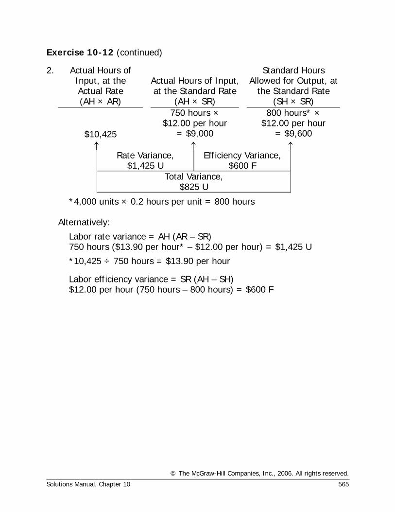
Exercise 10-12 (continued)
2. Actual Hours of Input, at the Actual Rate
Actual Hours of Input, at the Standard Rate
Standard Hours Allowed for Output, at
the Standard Rate (AH × AR) (AH × SR) (SH × SR) 750 hours ×
$12.00 per hour 800 hours* ×
$12.00 per hour $10,425 = $9,000 = $9,600 ↑ ↑ ↑
Rate Variance, $1,425 U
Efficiency Variance, $600 F
Total Variance, $825 U
*4,000 units × 0.2 hours per unit = 800 hours Alternatively:
Labor rate variance = AH (AR – SR) 750 hours ($13.90 per hour* – $12.00 per hour) = $1,425 U
*10,425 ÷ 750 hours = $13.90 per hour
Labor efficiency variance = SR (AH – SH) $12.00 per hour (750 hours – 800 hours) = $600 F
© The McGraw-Hill Companies, Inc., 2006. All rights reserved.
566 Managerial Accounting, 11th Edition
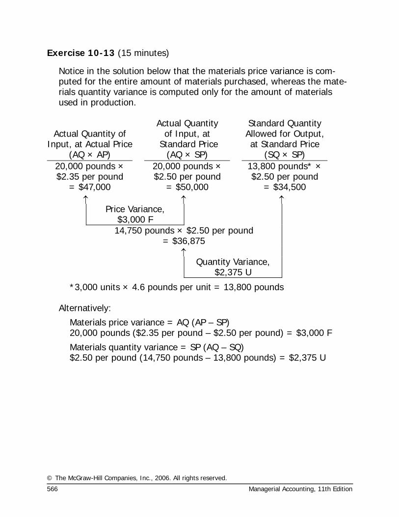
Exercise 10-13 (15 minutes)
Notice in the solution below that the materials price variance is com-puted for the entire amount of materials purchased, whereas the mate-rials quantity variance is computed only for the amount of materials used in production.
Actual Quantity of Input, at Actual Price
Actual Quantity of Input, at
Standard Price
Standard Quantity Allowed for Output, at Standard Price
(AQ × AP) (AQ × SP) (SQ × SP) 20,000 pounds × $2.35 per pound
20,000 pounds × $2.50 per pound
13,800 pounds* ×$2.50 per pound
= $47,000 = $50,000 = $34,500 ↑ ↑ ↑
Price Variance, $3,000 F
14,750 pounds × $2.50 per pound = $36,875
↑ Quantity Variance,
$2,375 U
*3,000 units × 4.6 pounds per unit = 13,800 pounds Alternatively:
Materials price variance = AQ (AP – SP) 20,000 pounds ($2.35 per pound – $2.50 per pound) = $3,000 F
Materials quantity variance = SP (AQ – SQ) $2.50 per pound (14,750 pounds – 13,800 pounds) = $2,375 U
© The McGraw-Hill Companies, Inc., 2006. All rights reserved.
Solutions Manual, Chapter 10 567
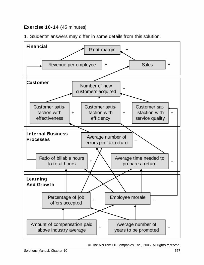
Exercise 10-14 (45 minutes)
1. Students’ answers may differ in some details from this solution.
Revenue per employee Sales
Profit margin Financial
Ratio of billable hours to total hours
Average number of errors per tax return
Average time needed to prepare a return
Percentage of job offers accepted
Employee morale
Amount of compensation paid above industry average
Average number of years to be promoted
Customer
Internal Business Processes
Learning And Growth
+ –
+ +
+
–
Customer satis-faction with effectiveness
Customer satis-faction with efficiency
Customer sat-isfaction with service quality
Number of new customers acquired
++ +
+
+ +
+
–
© The McGraw-Hill Companies, Inc., 2006. All rights reserved.
568 Managerial Accounting, 11th Edition
Exercise 10-14 (continued)
2. The hypotheses underlying the balanced scorecard are indicated by the arrows in the diagram. Reading from the bottom of the balanced score-card, the hypotheses are:
° If the amount of compensation paid above the industry average in-creases, then the percentage of job offers accepted and the level of employee morale will increase.
° If the average number of years to be promoted decreases, then the percentage of job offers accepted and the level of employee morale will increase.
° If the percentage of job offers accepted increases, then the ratio of billable hours to total hours should increase while the average num-ber of errors per tax return and the average time needed to prepare a return should decrease.
° If employee morale increases, then the ratio of billable hours to total hours should increase while the average number of errors per tax re-turn and the average time needed to prepare a return should de-crease.
° If employee morale increases, then the customer satisfaction with service quality should increase.
° If the ratio of billable hours to total hours increases, then the revenue per employee should increase.
° If the average number of errors per tax return decreases, then the customer satisfaction with effectiveness should increase.
° If the average time needed to prepare a return decreases, then the customer satisfaction with efficiency should increase.
° If the customer satisfaction with effectiveness, efficiency and service quality increases, then the number of new customers acquired should increase.
° If the number of new customers acquired increases, then sales should increase.
° If revenue per employee and sales increase, then the profit margin should increase.
© The McGraw-Hill Companies, Inc., 2006. All rights reserved.
Solutions Manual, Chapter 10 569
Exercise 10-14 (continued)
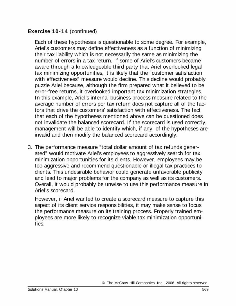
Each of these hypotheses is questionable to some degree. For example, Ariel’s customers may define effectiveness as a function of minimizing their tax liability which is not necessarily the same as minimizing the number of errors in a tax return. If some of Ariel’s customers became aware through a knowledgeable third party that Ariel overlooked legal tax minimizing opportunities, it is likely that the “customer satisfaction with effectiveness” measure would decline. This decline would probably puzzle Ariel because, although the firm prepared what it believed to be error-free returns, it overlooked important tax minimization strategies. In this example, Ariel’s internal business process measure related to the average number of errors per tax return does not capture all of the fac-tors that drive the customers’ satisfaction with effectiveness. The fact that each of the hypotheses mentioned above can be questioned does not invalidate the balanced scorecard. If the scorecard is used correctly, management will be able to identify which, if any, of the hypotheses are invalid and then modify the balanced scorecard accordingly.
3. The performance measure “total dollar amount of tax refunds gener-
ated” would motivate Ariel’s employees to aggressively search for tax minimization opportunities for its clients. However, employees may be too aggressive and recommend questionable or illegal tax practices to clients. This undesirable behavior could generate unfavorable publicity and lead to major problems for the company as well as its customers. Overall, it would probably be unwise to use this performance measure in Ariel’s scorecard.
However, if Ariel wanted to create a scorecard measure to capture this aspect of its client service responsibilities, it may make sense to focus the performance measure on its training process. Properly trained em-ployees are more likely to recognize viable tax minimization opportuni-ties.
© The McGraw-Hill Companies, Inc., 2006. All rights reserved.
570 Managerial Accounting, 11th Edition
Exercise 10-14 (continued)
4. Each office’s individual performance should be based on the scorecard measures only if the measures are controllable by those employed at the branch offices. In other words, it would not make sense to attempt to hold branch office managers responsible for measures such as the percent of job offers accepted or the amount of compensation paid above industry average. Recruiting and compensation decisions are not typically made at the branch offices. On the other hand, it would make sense to measure the branch offices with respect to internal business process, customer, and financial performance. Gathering this type of data would be useful for evaluating the performance of employees at each office.
© The McGraw-Hill Companies, Inc., 2006. All rights reserved.
Solutions Manual, Chapter 10 571
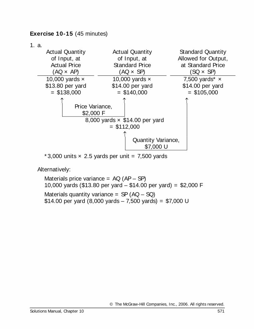
Exercise 10-15 (45 minutes)
1. a. Actual Quantity
of Input, at Actual Price
Actual Quantity of Input, at
Standard Price
Standard Quantity Allowed for Output, at Standard Price
(AQ × AP) (AQ × SP) (SQ × SP) 10,000 yards × $13.80 per yard
10,000 yards × $14.00 per yard
7,500 yards* × $14.00 per yard
= $138,000 = $140,000 = $105,000 ↑ ↑ ↑
Price Variance, $2,000 F
8,000 yards × $14.00 per yard = $112,000
↑ Quantity Variance,
$7,000 U
*3,000 units × 2.5 yards per unit = 7,500 yards Alternatively:
Materials price variance = AQ (AP – SP) 10,000 yards ($13.80 per yard – $14.00 per yard) = $2,000 F
Materials quantity variance = SP (AQ – SQ) $14.00 per yard (8,000 yards – 7,500 yards) = $7,000 U
© The McGraw-Hill Companies, Inc., 2006. All rights reserved.
572 Managerial Accounting, 11th Edition
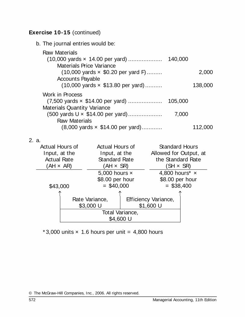
Exercise 10-15 (continued)
b. The journal entries would be:
Raw Materials (10,000 yards × 14.00 per yard) .................... 140,000
Materials Price Variance (10,000 yards × $0.20 per yard F)......... 2,000
Accounts Payable (10,000 yards × $13.80 per yard).......... 138,000
Work in Process (7,500 yards × $14.00 per yard) .................... 105,000
Materials Quantity Variance (500 yards U × $14.00 per yard).................... 7,000
Raw Materials (8,000 yards × $14.00 per yard)............ 112,000
2. a.
Actual Hours of Input, at the Actual Rate
Actual Hours of Input, at the
Standard Rate
Standard Hours Allowed for Output, at
the Standard Rate (AH × AR) (AH × SR) (SH × SR)
5,000 hours × $8.00 per hour
4,800 hours* × $8.00 per hour
$43,000 = $40,000 = $38,400 ↑ ↑ ↑
Rate Variance, $3,000 U
Efficiency Variance, $1,600 U
Total Variance, $4,600 U
*3,000 units × 1.6 hours per unit = 4,800 hours
© The McGraw-Hill Companies, Inc., 2006. All rights reserved.
Solutions Manual, Chapter 10 573
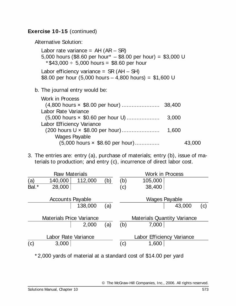
Exercise 10-15 (continued)
Alternative Solution:
Labor rate variance = AH (AR – SR) 5,000 hours ($8.60 per hour* – $8.00 per hour) = $3,000 U *$43,000 ÷ 5,000 hours = $8.60 per hour
Labor efficiency variance = SR (AH – SH) $8.00 per hour (5,000 hours – 4,800 hours) = $1,600 U b. The journal entry would be:
Work in Process (4,800 hours × $8.00 per hour) ....................... 38,400
Labor Rate Variance (5,000 hours × $0.60 per hour U) .................... 3,000
Labor Efficiency Variance (200 hours U × $8.00 per hour)....................... 1,600
Wages Payable (5,000 hours × $8.60 per hour)............... 43,000
3. The entries are: entry (a), purchase of materials; entry (b), issue of ma-
terials to production; and entry (c), incurrence of direct labor cost.
Raw Materials Work in Process (a) 140,000 112,000 (b) (b) 105,000Bal.* 28,000 (c) 38,400
Accounts Payable Wages Payable 138,000 (a) 43,000 (c)
Materials Price Variance Materials Quantity Variance 2,000 (a) (b) 7,000
Labor Rate Variance Labor Efficiency Variance (c) 3,000 (c) 1,600 *2,000 yards of material at a standard cost of $14.00 per yard
© The McGraw-Hill Companies, Inc., 2006. All rights reserved.
574 Managerial Accounting, 11th Edition
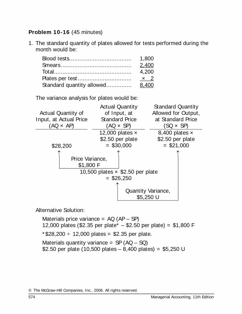
Problem 10-16 (45 minutes)
1. The standard quantity of plates allowed for tests performed during the month would be:
Blood tests..................................... 1,800Smears.......................................... 2,400Total.............................................. 4,200Plates per test................................ × 2Standard quantity allowed............... 8,400
The variance analysis for plates would be:
Actual Quantity of
Input, at Actual Price
Actual Quantity of Input, at
Standard Price
Standard Quantity Allowed for Output, at Standard Price
(AQ × AP) (AQ × SP) (SQ × SP) 12,000 plates ×
$2.50 per plate 8,400 plates ×
$2.50 per plate $28,200 = $30,000 = $21,000
↑ ↑ ↑ Price Variance,
$1,800 F
10,500 plates × $2.50 per plate = $26,250
↑ Quantity Variance,
$5,250 U Alternative Solution:
Materials price variance = AQ (AP – SP) 12,000 plates ($2.35 per plate* – $2.50 per plate) = $1,800 F
*$28,200 ÷ 12,000 plates = $2.35 per plate.
Materials quantity variance = SP (AQ – SQ) $2.50 per plate (10,500 plates – 8,400 plates) = $5,250 U
© The McGraw-Hill Companies, Inc., 2006. All rights reserved.
Solutions Manual, Chapter 10 575
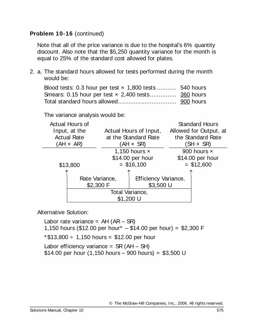
Problem 10-16 (continued)
Note that all of the price variance is due to the hospital’s 6% quantity discount. Also note that the $5,250 quantity variance for the month is equal to 25% of the standard cost allowed for plates.
2. a. The standard hours allowed for tests performed during the month
would be:
Blood tests: 0.3 hour per test × 1,800 tests ........... 540 hours Smears: 0.15 hour per test × 2,400 tests ............... 360 hours Total standard hours allowed................................. 900 hours
The variance analysis would be:
Actual Hours of Input, at the Actual Rate
Actual Hours of Input, at the Standard Rate
Standard Hours Allowed for Output, at
the Standard Rate (AH × AR) (AH × SR) (SH × SR)
1,150 hours × $14.00 per hour
900 hours × $14.00 per hour
$13,800 = $16,100 = $12,600 ↑ ↑ ↑
Rate Variance, $2,300 F
Efficiency Variance, $3,500 U
Total Variance, $1,200 U
Alternative Solution:
Labor rate variance = AH (AR – SR) 1,150 hours ($12.00 per hour* – $14.00 per hour) = $2,300 F
*$13,800 ÷ 1,150 hours = $12.00 per hour
Labor efficiency variance = SR (AH – SH) $14.00 per hour (1,150 hours – 900 hours) = $3,500 U
© The McGraw-Hill Companies, Inc., 2006. All rights reserved.
576 Managerial Accounting, 11th Edition
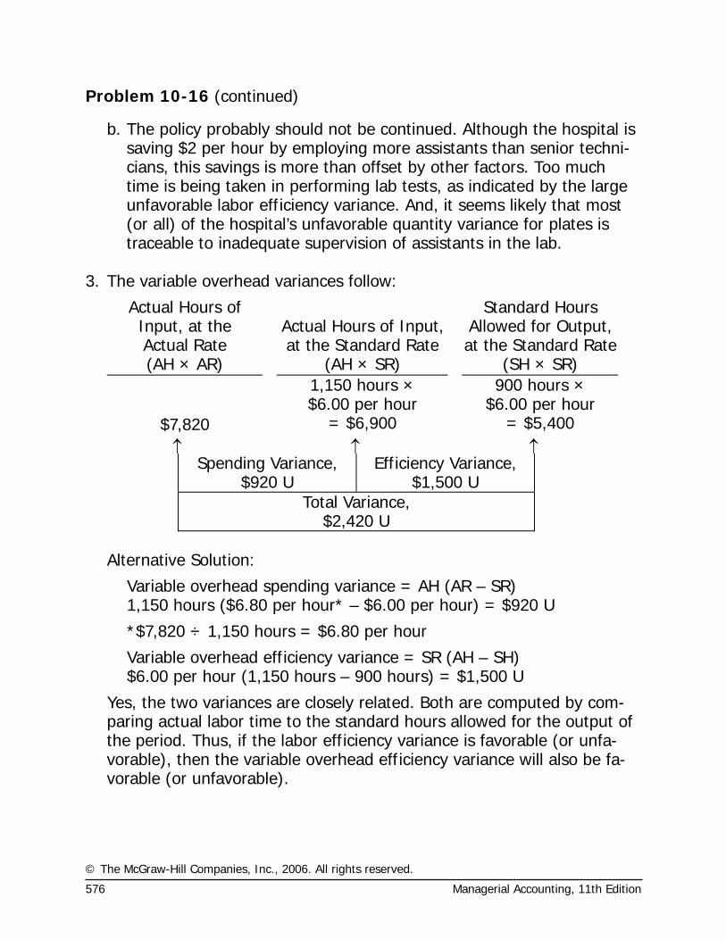
Problem 10-16 (continued)
b. The policy probably should not be continued. Although the hospital is saving $2 per hour by employing more assistants than senior techni-cians, this savings is more than offset by other factors. Too much time is being taken in performing lab tests, as indicated by the large unfavorable labor efficiency variance. And, it seems likely that most (or all) of the hospital’s unfavorable quantity variance for plates is traceable to inadequate supervision of assistants in the lab.
3. The variable overhead variances follow:
Actual Hours of Input, at the Actual Rate
Actual Hours of Input, at the Standard Rate
Standard Hours Allowed for Output, at the Standard Rate
(AH × AR) (AH × SR) (SH × SR) 1,150 hours ×
$6.00 per hour 900 hours ×
$6.00 per hour $7,820 = $6,900 = $5,400
↑ ↑ ↑ Spending Variance,
$920 U Efficiency Variance,
$1,500 U Total Variance,
$2,420 U Alternative Solution:
Variable overhead spending variance = AH (AR – SR) 1,150 hours ($6.80 per hour* – $6.00 per hour) = $920 U
*$7,820 ÷ 1,150 hours = $6.80 per hour
Variable overhead efficiency variance = SR (AH – SH) $6.00 per hour (1,150 hours – 900 hours) = $1,500 U
Yes, the two variances are closely related. Both are computed by com-paring actual labor time to the standard hours allowed for the output of the period. Thus, if the labor efficiency variance is favorable (or unfa-vorable), then the variable overhead efficiency variance will also be fa-vorable (or unfavorable).
© The McGraw-Hill Companies, Inc., 2006. All rights reserved.
Solutions Manual, Chapter 10 577
Problem 10-17 (45 minutes)
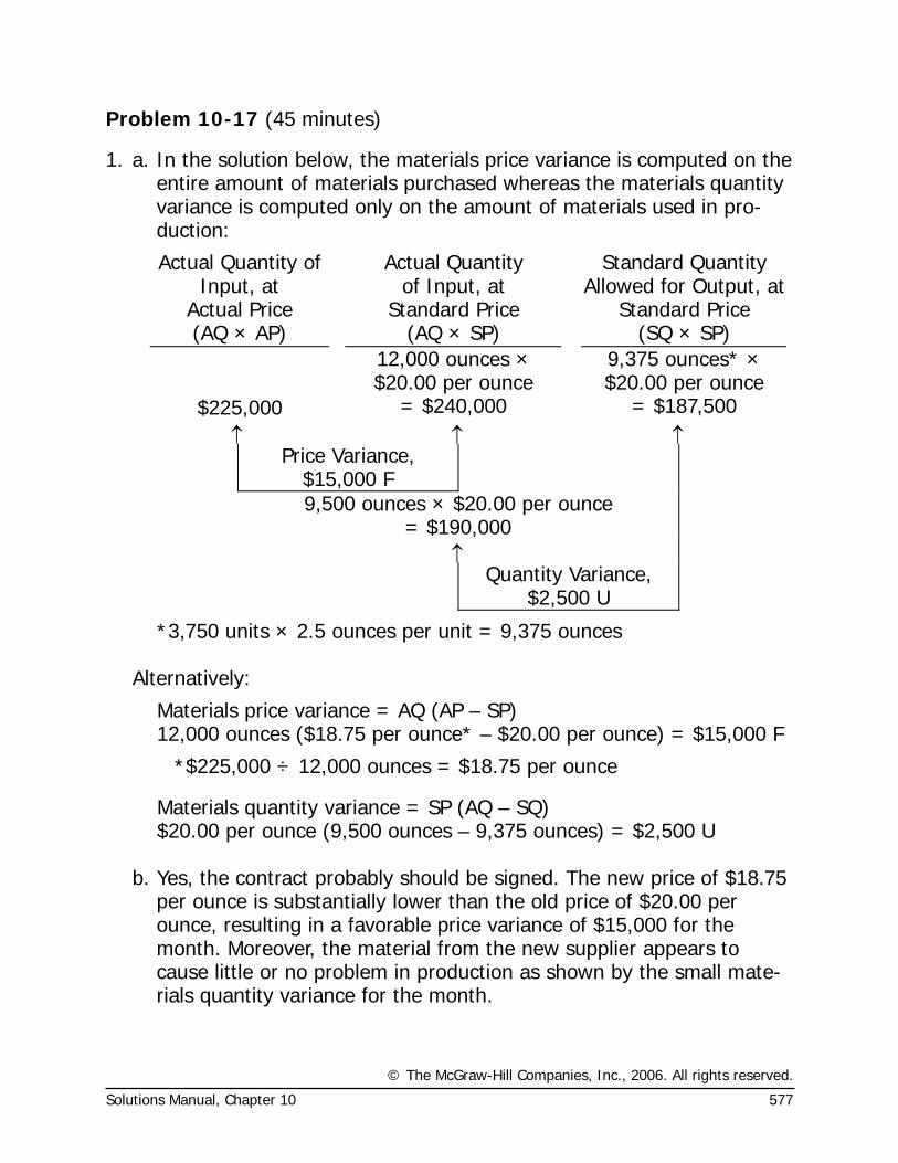
1. a. In the solution below, the materials price variance is computed on the entire amount of materials purchased whereas the materials quantity variance is computed only on the amount of materials used in pro-duction:
Actual Quantity of Input, at
Actual Price
Actual Quantity of Input, at
Standard Price
Standard Quantity Allowed for Output, at
Standard Price (AQ × AP) (AQ × SP) (SQ × SP)
12,000 ounces × $20.00 per ounce
9,375 ounces* × $20.00 per ounce
$225,000 = $240,000 = $187,500 ↑ ↑ ↑
Price Variance, $15,000 F
9,500 ounces × $20.00 per ounce = $190,000
↑ Quantity Variance,
$2,500 U
*3,750 units × 2.5 ounces per unit = 9,375 ounces Alternatively:
Materials price variance = AQ (AP – SP) 12,000 ounces ($18.75 per ounce* – $20.00 per ounce) = $15,000 F
*$225,000 ÷ 12,000 ounces = $18.75 per ounce
Materials quantity variance = SP (AQ – SQ) $20.00 per ounce (9,500 ounces – 9,375 ounces) = $2,500 U b. Yes, the contract probably should be signed. The new price of $18.75
per ounce is substantially lower than the old price of $20.00 per ounce, resulting in a favorable price variance of $15,000 for the month. Moreover, the material from the new supplier appears to cause little or no problem in production as shown by the small mate-rials quantity variance for the month.
© The McGraw-Hill Companies, Inc., 2006. All rights reserved.
578 Managerial Accounting, 11th Edition
Problem 10-17 (continued)
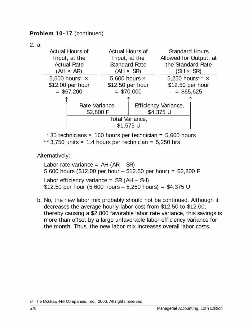
2. a. Actual Hours of Input, at the Actual Rate
Actual Hours of Input, at the
Standard Rate
Standard Hours Allowed for Output, at
the Standard Rate (AH × AR) (AH × SR) (SH × SR)
5,600 hours* × $12.00 per hour
5,600 hours × $12.50 per hour
5,250 hours** × $12.50 per hour
= $67,200 = $70,000 = $65,625 ↑ ↑ ↑
Rate Variance, $2,800 F
Efficiency Variance, $4,375 U
Total Variance, $1,575 U
* 35 technicians × 160 hours per technician = 5,600 hours ** 3,750 units × 1.4 hours per technician = 5,250 hrs
Alternatively:
Labor rate variance = AH (AR – SR) 5,600 hours ($12.00 per hour – $12.50 per hour) = $2,800 F
Labor efficiency variance = SR (AH – SH) $12.50 per hour (5,600 hours – 5,250 hours) = $4,375 U b. No, the new labor mix probably should not be continued. Although it
decreases the average hourly labor cost from $12.50 to $12.00, thereby causing a $2,800 favorable labor rate variance, this savings is more than offset by a large unfavorable labor efficiency variance for the month. Thus, the new labor mix increases overall labor costs.
© The McGraw-Hill Companies, Inc., 2006. All rights reserved.
Solutions Manual, Chapter 10 579
Problem 10-17 (continued)
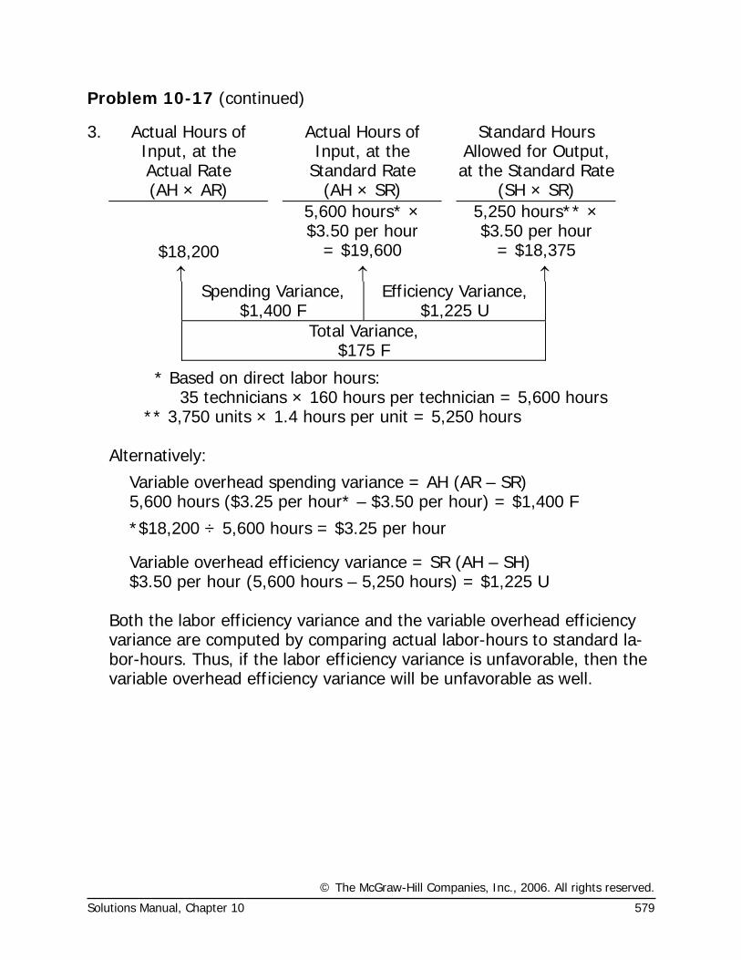
3. Actual Hours of Input, at the Actual Rate
Actual Hours of Input, at the
Standard Rate
Standard Hours Allowed for Output, at the Standard Rate
(AH × AR) (AH × SR) (SH × SR) 5,600 hours* ×
$3.50 per hour 5,250 hours** ×
$3.50 per hour $18,200 = $19,600 = $18,375 ↑ ↑ ↑
Spending Variance, $1,400 F
Efficiency Variance, $1,225 U
Total Variance, $175 F
* Based on direct labor hours: 35 technicians × 160 hours per technician = 5,600 hours ** 3,750 units × 1.4 hours per unit = 5,250 hours Alternatively:
Variable overhead spending variance = AH (AR – SR) 5,600 hours ($3.25 per hour* – $3.50 per hour) = $1,400 F
*$18,200 ÷ 5,600 hours = $3.25 per hour
Variable overhead efficiency variance = SR (AH – SH) $3.50 per hour (5,600 hours – 5,250 hours) = $1,225 U Both the labor efficiency variance and the variable overhead efficiency
variance are computed by comparing actual labor-hours to standard la-bor-hours. Thus, if the labor efficiency variance is unfavorable, then the variable overhead efficiency variance will be unfavorable as well.
© The McGraw-Hill Companies, Inc., 2006. All rights reserved.
580 Managerial Accounting, 11th Edition
Problem 10-18 (60 minutes)
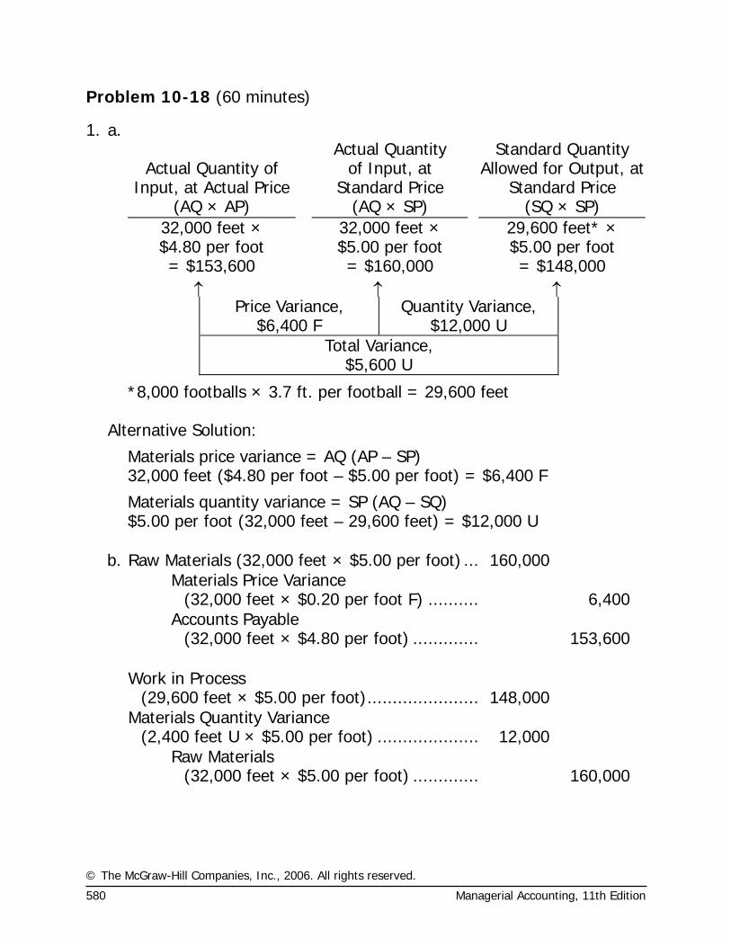
1. a.
Actual Quantity of Input, at Actual Price
Actual Quantity of Input, at
Standard Price
Standard Quantity Allowed for Output, at
Standard Price (AQ × AP) (AQ × SP) (SQ × SP)
32,000 feet × $4.80 per foot
32,000 feet × $5.00 per foot
29,600 feet* × $5.00 per foot
= $153,600 = $160,000 = $148,000 ↑ ↑ ↑
Price Variance, $6,400 F
Quantity Variance, $12,000 U
Total Variance, $5,600 U
*8,000 footballs × 3.7 ft. per football = 29,600 feet Alternative Solution:
Materials price variance = AQ (AP – SP) 32,000 feet ($4.80 per foot – $5.00 per foot) = $6,400 F
Materials quantity variance = SP (AQ – SQ) $5.00 per foot (32,000 feet – 29,600 feet) = $12,000 U
b. Raw Materials (32,000 feet × $5.00 per foot) ... 160,000
Materials Price Variance
(32,000 feet × $0.20 per foot F) .......... 6,400
Accounts Payable
(32,000 feet × $4.80 per foot) ............. 153,600
Work in Process
(29,600 feet × $5.00 per foot)...................... 148,000
Materials Quantity Variance
(2,400 feet U × $5.00 per foot) .................... 12,000
Raw Materials
(32,000 feet × $5.00 per foot) ............. 160,000
© The McGraw-Hill Companies, Inc., 2006. All rights reserved.
Solutions Manual, Chapter 10 581
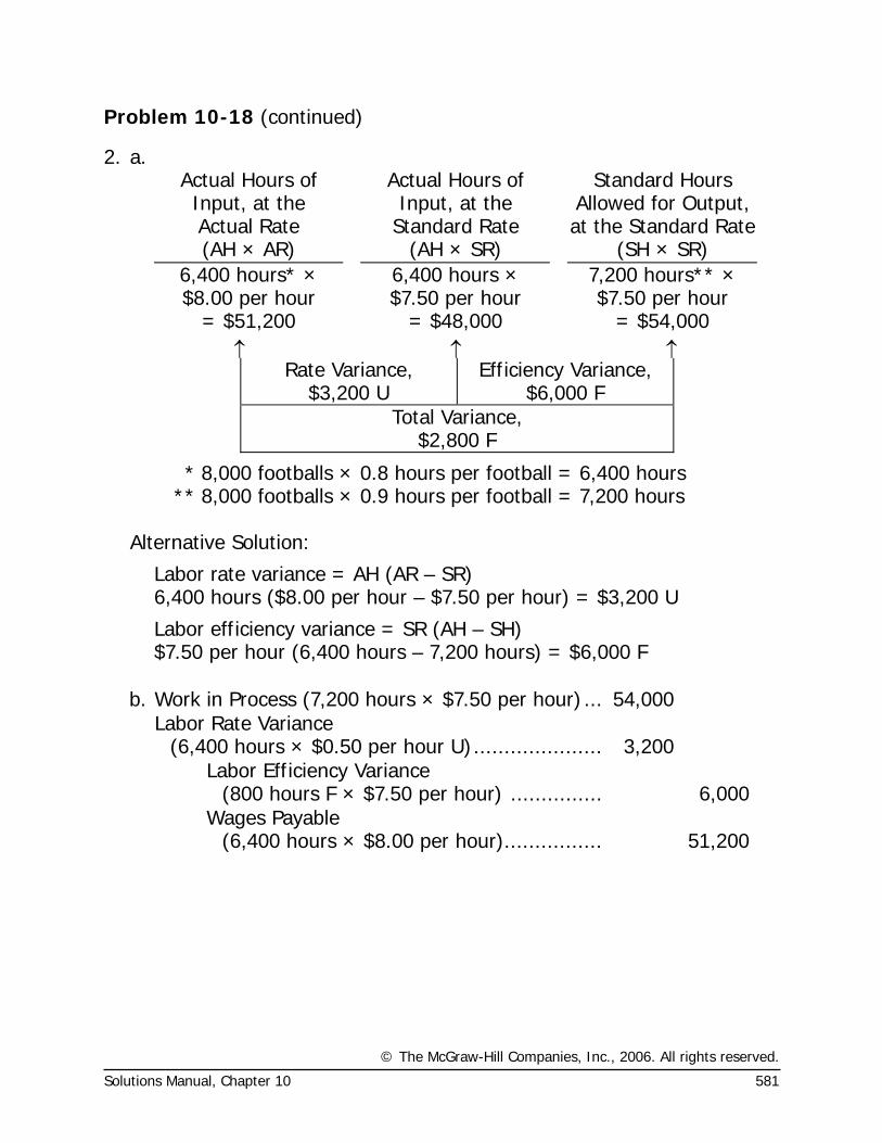
Problem 10-18 (continued)
2. a. Actual Hours of Input, at the Actual Rate
Actual Hours of Input, at the
Standard Rate
Standard Hours Allowed for Output, at the Standard Rate
(AH × AR) (AH × SR) (SH × SR) 6,400 hours* × $8.00 per hour
6,400 hours × $7.50 per hour
7,200 hours** × $7.50 per hour
= $51,200 = $48,000 = $54,000 ↑ ↑ ↑
Rate Variance, $3,200 U
Efficiency Variance, $6,000 F
Total Variance, $2,800 F
* 8,000 footballs × 0.8 hours per football = 6,400 hours ** 8,000 footballs × 0.9 hours per football = 7,200 hours
Alternative Solution:
Labor rate variance = AH (AR – SR) 6,400 hours ($8.00 per hour – $7.50 per hour) = $3,200 U
Labor efficiency variance = SR (AH – SH) $7.50 per hour (6,400 hours – 7,200 hours) = $6,000 F
b. Work in Process (7,200 hours × $7.50 per hour) ... 54,000
Labor Rate Variance
(6,400 hours × $0.50 per hour U)..................... 3,200
Labor Efficiency Variance
(800 hours F × $7.50 per hour) ............... 6,000
Wages Payable
(6,400 hours × $8.00 per hour)................ 51,200
© The McGraw-Hill Companies, Inc., 2006. All rights reserved.
582 Managerial Accounting, 11th Edition
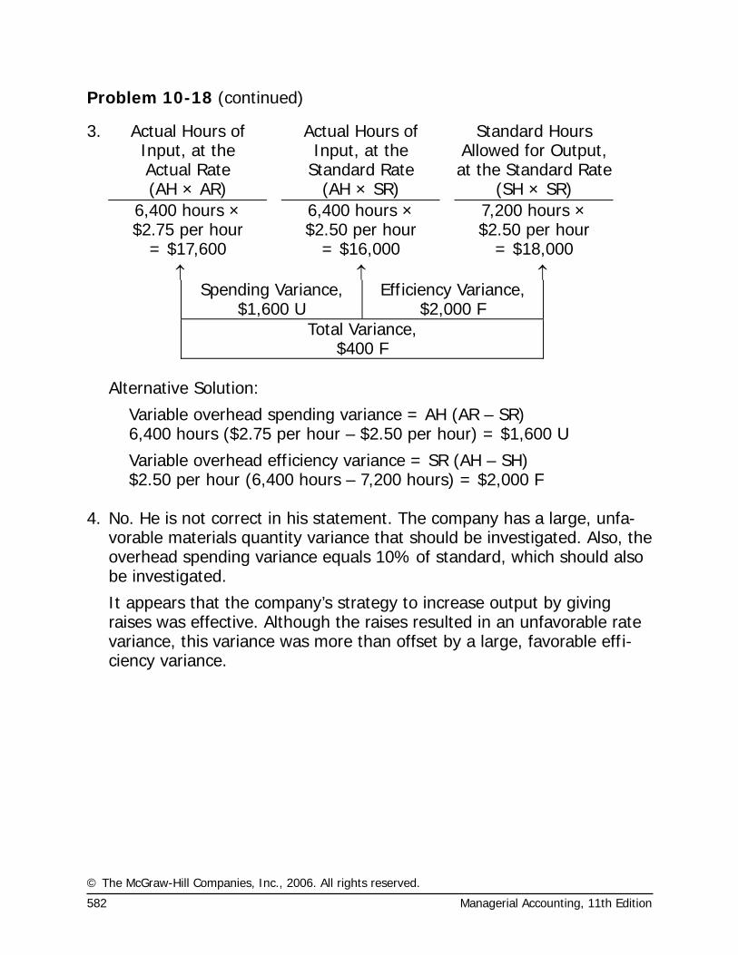
Problem 10-18 (continued)
3. Actual Hours of Input, at the Actual Rate
Actual Hours of Input, at the
Standard Rate
Standard Hours Allowed for Output, at the Standard Rate
(AH × AR) (AH × SR) (SH × SR) 6,400 hours ×
$2.75 per hour 6,400 hours ×
$2.50 per hour 7,200 hours ×
$2.50 per hour = $17,600 = $16,000 = $18,000 ↑ ↑ ↑
Spending Variance, $1,600 U
Efficiency Variance, $2,000 F
Total Variance, $400 F
Alternative Solution:
Variable overhead spending variance = AH (AR – SR) 6,400 hours ($2.75 per hour – $2.50 per hour) = $1,600 U
Variable overhead efficiency variance = SR (AH – SH) $2.50 per hour (6,400 hours – 7,200 hours) = $2,000 F 4. No. He is not correct in his statement. The company has a large, unfa-
vorable materials quantity variance that should be investigated. Also, the overhead spending variance equals 10% of standard, which should also be investigated.
It appears that the company’s strategy to increase output by giving raises was effective. Although the raises resulted in an unfavorable rate variance, this variance was more than offset by a large, favorable effi-ciency variance.
© The McGraw-Hill Companies, Inc., 2006. All rights reserved.
Solutions Manual, Chapter 10 583
Problem 10-18 (continued)
5. The variances have many possible causes. Some of the more likely causes include the following:
Materials variances:
Favorable price variance: Fortunate purchase, inferior quality materials, unusual discount due to quantity purchased, drop in market price, less costly method of freight, outdated or inaccurate standards.
Unfavorable quantity variance: Carelessness, poorly adjusted machines, unskilled workers, inferior quality materials, outdated or inaccurate stan-dards.
Labor variances:
Unfavorable rate variance: Use of highly skilled workers, change in pay scale, overtime, outdated or inaccurate standards.
Favorable efficiency variance: Use of highly skilled workers, high quality materials, new equipment, outdated or inaccurate standards.
Variable overhead variances:
Unfavorable spending variance: Increase in costs, waste, theft, spillage, purchases in uneconomical lots, outdated or inaccurate standards.
Favorable efficiency variance: Same as for labor efficiency variance.
© The McGraw-Hill Companies, Inc., 2006. All rights reserved.
584 Managerial Accounting, 11th Edition
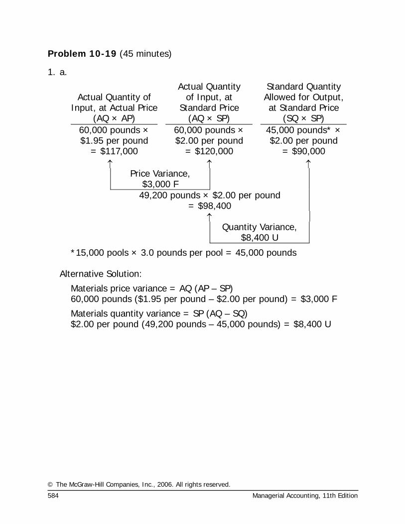
Problem 10-19 (45 minutes)
1. a.
Actual Quantity of
Input, at Actual Price
Actual Quantity of Input, at
Standard Price
Standard Quantity Allowed for Output, at Standard Price
(AQ × AP) (AQ × SP) (SQ × SP) 60,000 pounds × $1.95 per pound
60,000 pounds × $2.00 per pound
45,000 pounds* × $2.00 per pound
= $117,000 = $120,000 = $90,000 ↑ ↑ ↑
Price Variance, $3,000 F
49,200 pounds × $2.00 per pound = $98,400
↑ Quantity Variance,
$8,400 U
*15,000 pools × 3.0 pounds per pool = 45,000 pounds Alternative Solution:
Materials price variance = AQ (AP – SP) 60,000 pounds ($1.95 per pound – $2.00 per pound) = $3,000 F
Materials quantity variance = SP (AQ – SQ) $2.00 per pound (49,200 pounds – 45,000 pounds) = $8,400 U
© The McGraw-Hill Companies, Inc., 2006. All rights reserved.
Solutions Manual, Chapter 10 585
Problem 10-19 (continued)
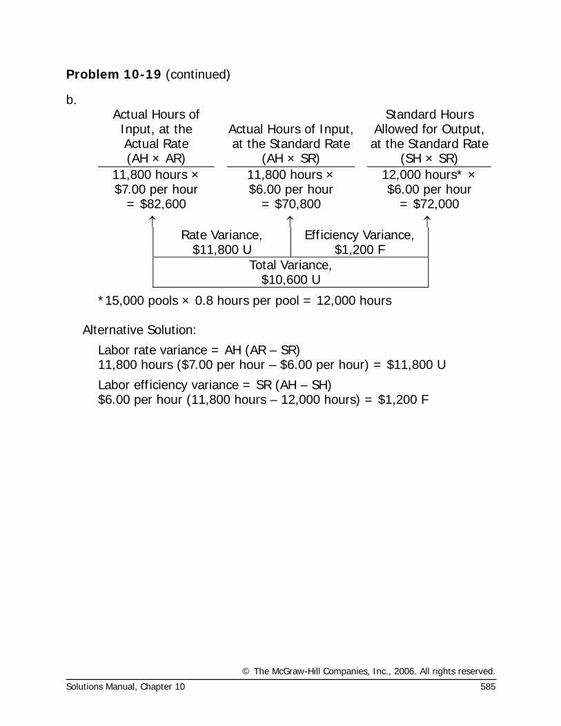
b. Actual Hours of Input, at the Actual Rate
Actual Hours of Input, at the Standard Rate
Standard Hours Allowed for Output, at the Standard Rate
(AH × AR) (AH × SR) (SH × SR) 11,800 hours × $7.00 per hour
11,800 hours × $6.00 per hour
12,000 hours* × $6.00 per hour
= $82,600 = $70,800 = $72,000 ↑ ↑ ↑
Rate Variance, $11,800 U
Efficiency Variance, $1,200 F
Total Variance, $10,600 U
*15,000 pools × 0.8 hours per pool = 12,000 hours Alternative Solution:
Labor rate variance = AH (AR – SR) 11,800 hours ($7.00 per hour – $6.00 per hour) = $11,800 U
Labor efficiency variance = SR (AH – SH) $6.00 per hour (11,800 hours – 12,000 hours) = $1,200 F
© The McGraw-Hill Companies, Inc., 2006. All rights reserved.
586 Managerial Accounting, 11th Edition
Problem 10-19 (continued)
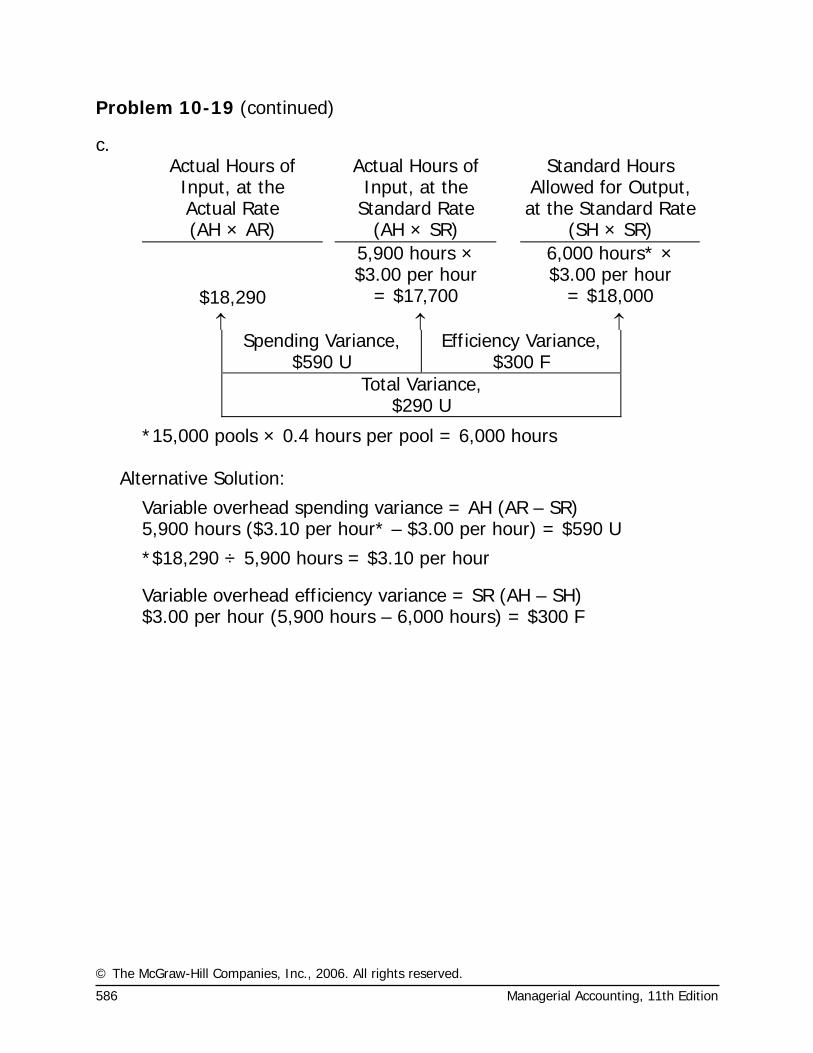
c. Actual Hours of Input, at the Actual Rate
Actual Hours of Input, at the
Standard Rate
Standard Hours Allowed for Output, at the Standard Rate
(AH × AR) (AH × SR) (SH × SR) 5,900 hours ×
$3.00 per hour 6,000 hours* ×
$3.00 per hour $18,290 = $17,700 = $18,000
↑ ↑ ↑ Spending Variance,
$590 U Efficiency Variance,
$300 F Total Variance,
$290 U
*15,000 pools × 0.4 hours per pool = 6,000 hours Alternative Solution:
Variable overhead spending variance = AH (AR – SR) 5,900 hours ($3.10 per hour* – $3.00 per hour) = $590 U
*$18,290 ÷ 5,900 hours = $3.10 per hour
Variable overhead efficiency variance = SR (AH – SH) $3.00 per hour (5,900 hours – 6,000 hours) = $300 F
© The McGraw-Hill Companies, Inc., 2006. All rights reserved.
Solutions Manual, Chapter 10 587
Problem 10-19 (continued)
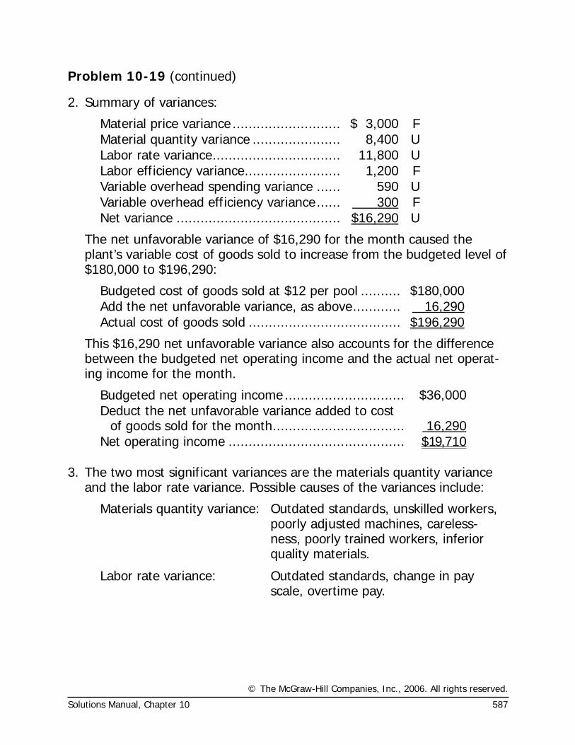
2. Summary of variances:
Material price variance ........................... $ 3,000 F Material quantity variance ...................... 8,400 U Labor rate variance................................ 11,800 U Labor efficiency variance........................ 1,200 F Variable overhead spending variance ...... 590 U Variable overhead efficiency variance...... 300 F Net variance ......................................... $16,290 U
The net unfavorable variance of $16,290 for the month caused the plant’s variable cost of goods sold to increase from the budgeted level of $180,000 to $196,290:
Budgeted cost of goods sold at $12 per pool .......... $180,000Add the net unfavorable variance, as above............ 16,290Actual cost of goods sold ...................................... $196,290
This $16,290 net unfavorable variance also accounts for the difference between the budgeted net operating income and the actual net operat-ing income for the month.
Budgeted net operating income.............................. $36,000Deduct the net unfavorable variance added to cost
of goods sold for the month................................. 16,290Net operating income ............................................ $19,710
3. The two most significant variances are the materials quantity variance
and the labor rate variance. Possible causes of the variances include:
Materials quantity variance: Outdated standards, unskilled workers, poorly adjusted machines, careless-ness, poorly trained workers, inferior quality materials.
Labor rate variance: Outdated standards, change in pay scale, overtime pay.
© The McGraw-Hill Companies, Inc., 2006. All rights reserved.
588 Managerial Accounting, 11th Edition
Problem 10-20 (60 minutes)
1. Both companies view training as important; both companies need to leverage technology to succeed in the marketplace; and both companies are concerned with minimizing defects. There are numerous differences between the two companies. For example, Applied Pharmaceuticals is a product-focused company and Destination Resorts International (DRI) is a service-focused company. Applied Pharmaceuticals’ training resources are focused on their engineers because they hold the key to the success of the organization. DRI’s training resources are focused on their front-line employees because they hold the key to the success of their organi-zation. Applied Pharmaceuticals’ technology investments are focused on supporting the innovation that is inherent in the product development side of the business. DRI’s technology investments are focused on sup-porting the day-to-day execution that is inherent in the customer inter-face side of the business. Applied Pharmaceuticals defines a defect from an internal manufacturing standpoint, while DRI defines a defect from an external customer interaction standpoint.
© The McGraw-Hill Companies, Inc., 2006. All rights reserved.
Solutions Manual, Chapter 10 589
Problem 10-20 (continued)
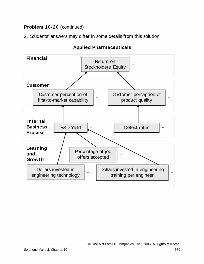
2. Students’ answers may differ in some details from this solution.
Applied Pharmaceuticals
Return on Stockholders’ Equity
Financial
Customer perception of first-to-market capability
Customer perception of product quality
Customer
R&D Yield Defect rates Internal Business Process
Dollars invested in engineering technology
Percentage of job offers accepted
Dollars invested in engineering training per engineer
Learning and Growth
+
+ +
+ –
+ +
+
© The McGraw-Hill Companies, Inc., 2006. All rights reserved.
590 Managerial Accounting, 11th Edition
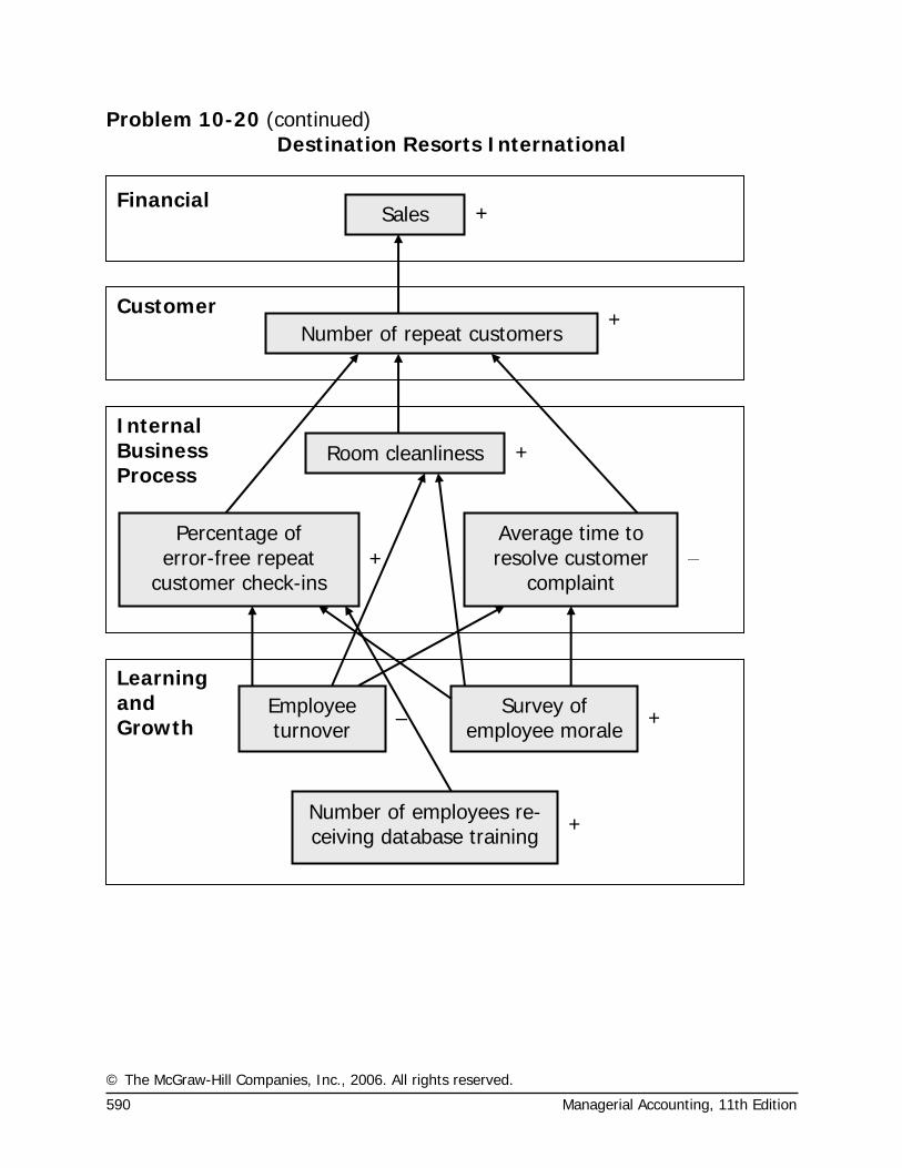
Problem 10-20 (continued) Destination Resorts International
SalesFinancial
Number of repeat customersCustomer
Percentage of error-free repeat
customer check-ins
Average time to resolve customer
complaint
Room cleanlinessInternal Business Process
Number of employees re-ceiving database training
Employee turnover
Survey of employee morale
Learning and Growth –
+
+
+
+
–
+
+
© The McGraw-Hill Companies, Inc., 2006. All rights reserved.
Solutions Manual, Chapter 10 591
Problem 10-20 (continued)
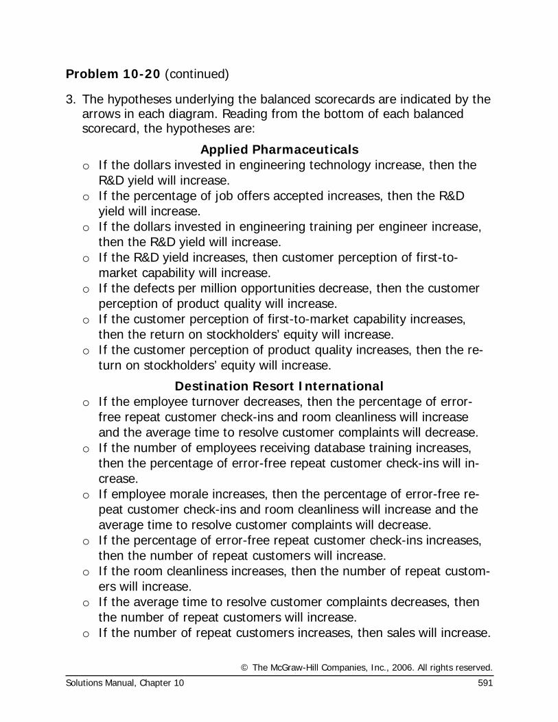
3. The hypotheses underlying the balanced scorecards are indicated by the arrows in each diagram. Reading from the bottom of each balanced scorecard, the hypotheses are:
Applied Pharmaceuticals o If the dollars invested in engineering technology increase, then the
R&D yield will increase. o If the percentage of job offers accepted increases, then the R&D
yield will increase. o If the dollars invested in engineering training per engineer increase,
then the R&D yield will increase. o If the R&D yield increases, then customer perception of first-to-
market capability will increase. o If the defects per million opportunities decrease, then the customer
perception of product quality will increase. o If the customer perception of first-to-market capability increases,
then the return on stockholders’ equity will increase. o If the customer perception of product quality increases, then the re-
turn on stockholders’ equity will increase.
Destination Resort International o If the employee turnover decreases, then the percentage of error-
free repeat customer check-ins and room cleanliness will increase and the average time to resolve customer complaints will decrease.
o If the number of employees receiving database training increases, then the percentage of error-free repeat customer check-ins will in-crease.
o If employee morale increases, then the percentage of error-free re-peat customer check-ins and room cleanliness will increase and the average time to resolve customer complaints will decrease.
o If the percentage of error-free repeat customer check-ins increases, then the number of repeat customers will increase.
o If the room cleanliness increases, then the number of repeat custom-ers will increase.
o If the average time to resolve customer complaints decreases, then the number of repeat customers will increase.
o If the number of repeat customers increases, then sales will increase.
© The McGraw-Hill Companies, Inc., 2006. All rights reserved.
592 Managerial Accounting, 11th Edition
Problem 10-20 (continued)
Each of these hypotheses is questionable to some degree. For example, in the case of Applied Pharmaceuticals, R&D yield is not the sole driver of the customers’ perception of first-to-market capability. More specifi-cally, if Applied Pharmaceuticals experimented with nine possible drug compounds in year one and three of those compounds proved to be successful in the marketplace it would result in an R&D yield of 33%. If in year two, it experimented with four possible drug compounds and two of those compounds proved to be successful in the marketplace it would result in an R&D yield of 50%. While the R&D yield has increased from year one to year two, it is quite possible that the customer’s per-ception of first-to-market capability would decrease. The fact that each of the hypotheses mentioned above can be questioned does not invali-date the balanced scorecard. If the scorecard is used correctly, man-agement will be able to identify which, if any, of the hypotheses are in-valid and the balanced scorecard can then be appropriately modified.
© The McGraw-Hill Companies, Inc., 2006. All rights reserved.
Solutions Manual, Chapter 10 593
Problem 10-21 (30 minutes)
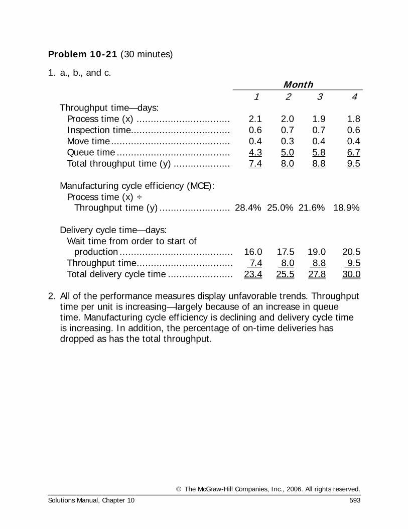
1. a., b., and c. Month
1 2 3 4 Throughput time—days:
Process time (x) ................................. 2.1 2.0 1.9 1.8Inspection time................................... 0.6 0.7 0.7 0.6Move time.......................................... 0.4 0.3 0.4 0.4Queue time ........................................ 4.3 5.0 5.8 6.7Total throughput time (y) .................... 7.4 8.0 8.8 9.5
Manufacturing cycle efficiency (MCE):
Process time (x) ÷ Throughput time (y) ......................... 28.4% 25.0% 21.6% 18.9%
Delivery cycle time—days:
Wait time from order to start of production ........................................ 16.0 17.5 19.0 20.5
Throughput time.................................. 7.4 8.0 8.8 9.5Total delivery cycle time ....................... 23.4 25.5 27.8 30.0
2. All of the performance measures display unfavorable trends. Throughput
time per unit is increasing—largely because of an increase in queue time. Manufacturing cycle efficiency is declining and delivery cycle time is increasing. In addition, the percentage of on-time deliveries has dropped as has the total throughput.
© The McGraw-Hill Companies, Inc., 2006. All rights reserved.
594 Managerial Accounting, 11th Edition
Problem 10-21 (continued)
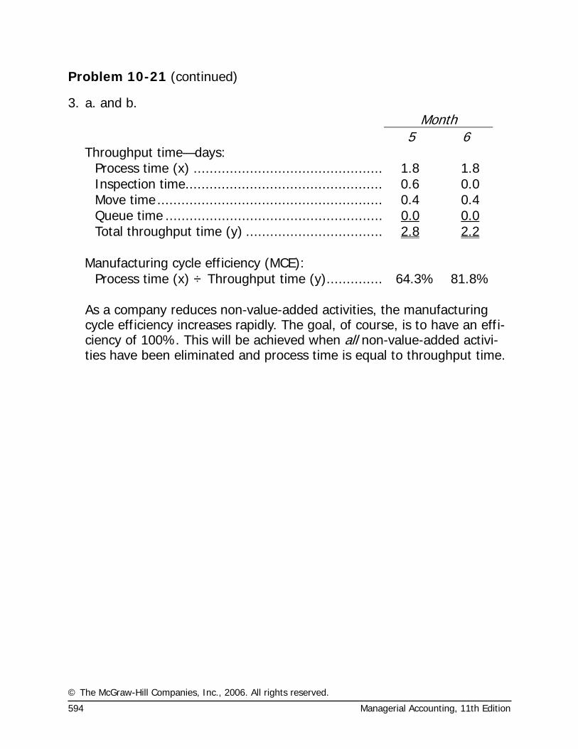
3. a. and b. Month
5 6 Throughput time—days:
Process time (x) ............................................... 1.8 1.8 Inspection time................................................. 0.6 0.0 Move time........................................................ 0.4 0.4 Queue time ...................................................... 0.0 0.0 Total throughput time (y) .................................. 2.8 2.2
Manufacturing cycle efficiency (MCE):
Process time (x) ÷ Throughput time (y).............. 64.3% 81.8% As a company reduces non-value-added activities, the manufacturing
cycle efficiency increases rapidly. The goal, of course, is to have an effi-ciency of 100%. This will be achieved when all non-value-added activi-ties have been eliminated and process time is equal to throughput time.
© The McGraw-Hill Companies, Inc., 2006. All rights reserved.
Solutions Manual, Chapter 10 595
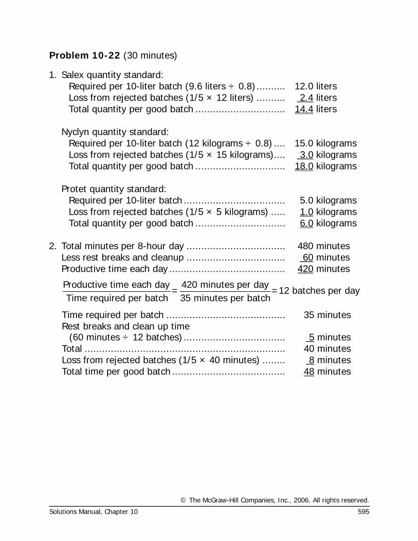
Problem 10-22 (30 minutes)
1. Salex quantity standard: Required per 10-liter batch (9.6 liters ÷ 0.8).......... 12.0 liters Loss from rejected batches (1/5 × 12 liters) .......... 2.4 liters Total quantity per good batch ............................... 14.4 liters Nyclyn quantity standard: Required per 10-liter batch (12 kilograms ÷ 0.8) .... 15.0 kilograms Loss from rejected batches (1/5 × 15 kilograms).... 3.0 kilograms Total quantity per good batch ............................... 18.0 kilograms Protet quantity standard: Required per 10-liter batch ................................... 5.0 kilograms Loss from rejected batches (1/5 × 5 kilograms) ..... 1.0 kilograms Total quantity per good batch ............................... 6.0 kilograms 2. Total minutes per 8-hour day .................................. 480 minutes Less rest breaks and cleanup .................................. 60 minutes Productive time each day ........................................ 420 minutes
Productive time each day 420 minutes per day= =12 batches per day
Time required per batch 35 minutes per batch
Time required per batch ......................................... 35 minutes
Rest breaks and clean up time
(60 minutes ÷ 12 batches) ................................... 5 minutes Total ..................................................................... 40 minutes Loss from rejected batches (1/5 × 40 minutes) ........ 8 minutes Total time per good batch ....................................... 48 minutes
© The McGraw-Hill Companies, Inc., 2006. All rights reserved.
596 Managerial Accounting, 11th Edition
Problem 10-22 (continued)
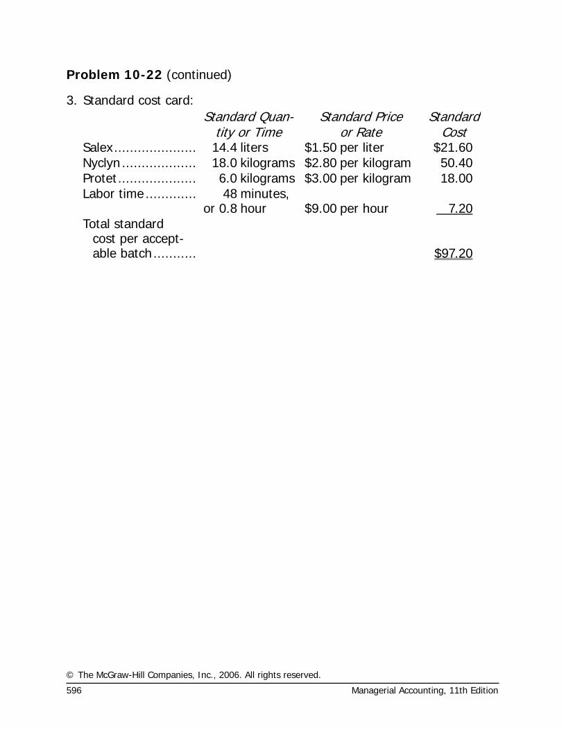
3. Standard cost card:
Standard Quan-
tity or Time Standard Price
or Rate Standard
Cost Salex..................... 14.4 liters $1.50 per liter $21.60 Nyclyn ................... 18.0 kilograms $2.80 per kilogram 50.40 Protet.................... 6.0 kilograms $3.00 per kilogram 18.00 Labor time ............. 48
or 0.8minutes, hour $9.00 per hour 7.20
Total standard cost per accept-able batch........... $97.20
© The McGraw-Hill Companies, Inc., 2006. All rights reserved.
Solutions Manual, Chapter 10 597
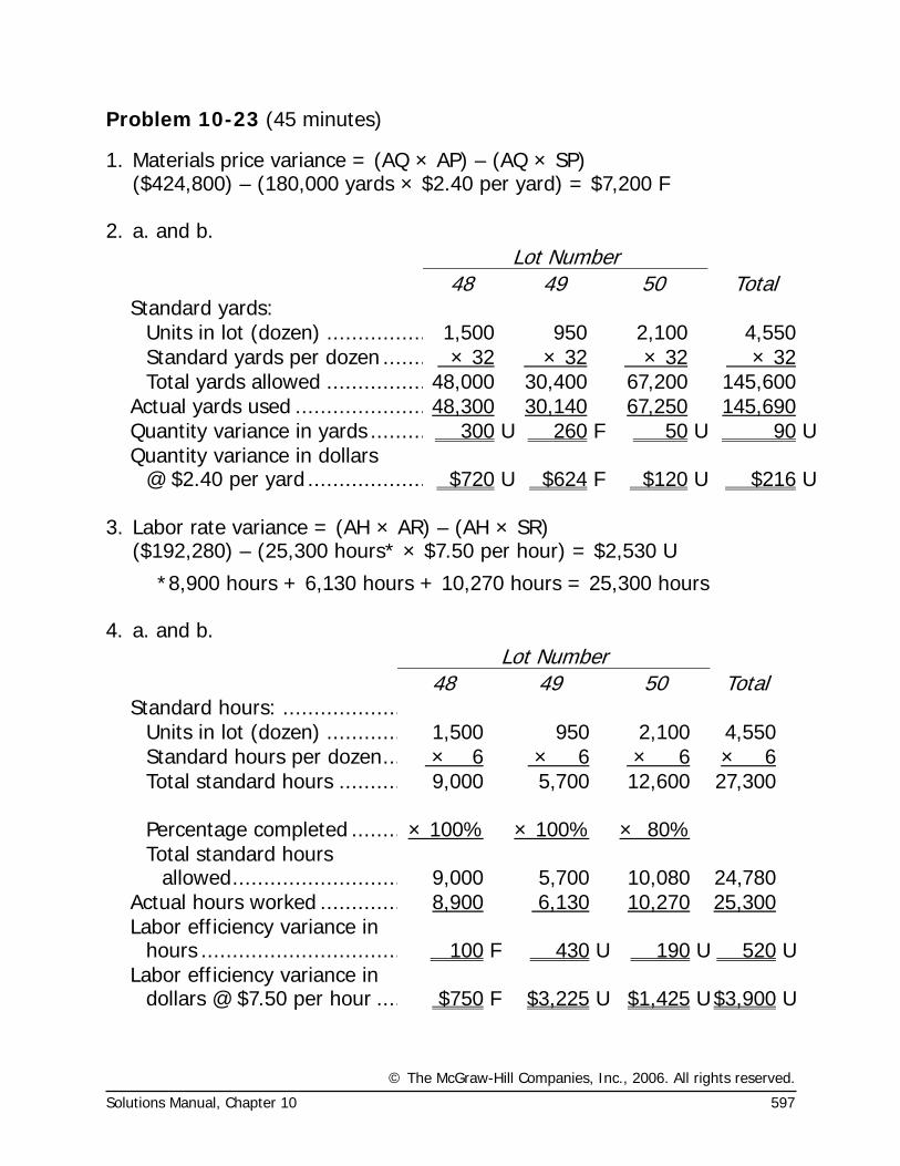
Problem 10-23 (45 minutes)
1. Materials price variance = (AQ × AP) – (AQ × SP) ($424,800) – (180,000 yards × $2.40 per yard) = $7,200 F 2. a. and b.
Lot Number 48 49 50 Total Standard yards:
Units in lot (dozen) ................ 1,500 950 2,100 4,550 Standard yards per dozen ....... × 32 × 32 × 32 × 32 Total yards allowed ................ 48,000 30,400 67,200 145,600
Actual yards used ..................... 48,300 30,140 67,250 145,690 Quantity variance in yards ......... 300 U 260 F 50 U 90 UQuantity variance in dollars
@ $2.40 per yard ................... $720 U $624 F $120 U $216 U 3. Labor rate variance = (AH × AR) – (AH × SR) ($192,280) – (25,300 hours* × $7.50 per hour) = $2,530 U
*8,900 hours + 6,130 hours + 10,270 hours = 25,300 hours 4. a. and b.
Lot Number 48 49 50 Total Standard hours: ...................
Units in lot (dozen) ............ 1,500 950 2,100 4,550 Standard hours per dozen... × 6 × 6 × 6 × 6 Total standard hours .......... 9,000 5,700 12,600 27,300
Percentage completed ........ × 100% × 100%
× 80% Total standard hours
allowed........................... 9,000 5,700 10,080 24,780 Actual hours worked ............. 8,900 6,130 10,270 25,300 Labor efficiency variance in
hours ................................ 100 F 430 U 190 U 520 ULabor efficiency variance in
dollars @ $7.50 per hour .... $750 F $3,225 U $1,425 U $3,900 U
© The McGraw-Hill Companies, Inc., 2006. All rights reserved.
598 Managerial Accounting, 11th Edition
Problem 10-23 (continued)
5. Some supervisors and managers rarely deal with, or think in terms of, dollars in their daily work. Instead they think in terms of hours, units, efficiency, and so on. For these managers, it may be better to express quantity variances in units (hours, yards, etc.) rather than in dollars. For other managers, quantity variances expressed in terms of dollars may be more useful—particularly to convey a notion of the materiality of the variance. In some cases, managers may prefer that the variances be expressed in terms of both dollars and units.
On the other hand, price variances expressed in units (hours, yards) would make little sense. Such variances should always be expressed in dollars.
© The McGraw-Hill Companies, Inc., 2006. All rights reserved.
Solutions Manual, Chapter 10 599
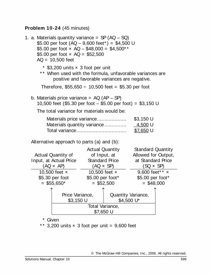
Problem 10-24 (45 minutes)
1. a. Materials quantity variance = SP (AQ – SQ) $5.00 per foot (AQ – 9,600 feet*) = $4,500 U $5.00 per foot × AQ – $48,000 = $4,500** $5.00 per foot × AQ = $52,500 AQ = 10,500 feet
* $3,200 units × 3 foot per unit ** When used with the formula, unfavorable variances are
positive and favorable variances are negative.
Therefore, $55,650 ÷ 10,500 feet = $5.30 per foot b. Materials price variance = AQ (AP – SP) 10,500 feet ($5.30 per foot – $5.00 per foot) = $3,150 U
The total variance for materials would be:
Materials price variance.................... $3,150 U Materials quantity variance ............... 4,500 U Total variance.................................. $7,650 U
Alternative approach to parts (a) and (b):
Actual Quantity of
Input, at Actual Price
Actual Quantity of Input, at
Standard Price
Standard Quantity Allowed for Output, at Standard Price
(AQ × AP) (AQ × SP) (SQ × SP) 10,500 feet × $5.30 per foot
10,500 feet × $5.00 per foot*
9,600 feet** × $5.00 per foot*
= $55,650* = $52,500 = $48,000 ↑ ↑ ↑
Price Variance, $3,150 U
Quantity Variance, $4,500 U*
Total Variance, $7,650 U
* Given ** 3,200 units × 3 foot per unit = 9,600 feet
© The McGraw-Hill Companies, Inc., 2006. All rights reserved.
600 Managerial Accounting, 11th Edition
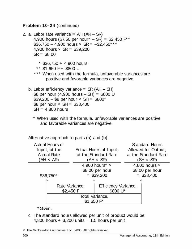
Problem 10-24 (continued)
2. a. Labor rate variance = AH (AR – SR) 4,900 hours ($7.50 per hour* – SR) = $2,450 F** $36,750 – 4,900 hours × SR = –$2,450*** 4,900 hours × SR = $39,200 SR = $8.00
* $36,750 ÷ 4,900 hours ** $1,650 F + $800 U.
*** When used with the formula, unfavorable variances are positive and favorable variances are negative.
b. Labor efficiency variance = SR (AH – SH) $8 per hour (4,900 hours – SH) = $800 U $39,200 – $8 per hour × SH = $800* $8 per hour × SH = $38,400 SH = 4,800 hours
* When used with the formula, unfavorable variances are positive and favorable variances are negative.
Alternative approach to parts (a) and (b):
Actual Hours of Input, at the Actual Rate
Actual Hours of Input, at the Standard Rate
Standard Hours Allowed for Output, at the Standard Rate
(AH × AR) (AH × SR) (SH × SR) 4,900 hours* ×
$8.00 per hour 4,800 hours ×
$8.00 per hour $36,750* = $39,200 = $38,400
↑ ↑ ↑ Rate Variance,
$2,450 F Efficiency Variance,
$800 U* Total Variance,
$1,650 F*
*Given.
c. The standard hours allowed per unit of product would be: 4,800 hours ÷ 3,200 units = 1.5 hours per unit
© The McGraw-Hill Companies, Inc., 2006. All rights reserved.
Solutions Manual, Chapter 10 601
Problem 10-25 (75 minutes)
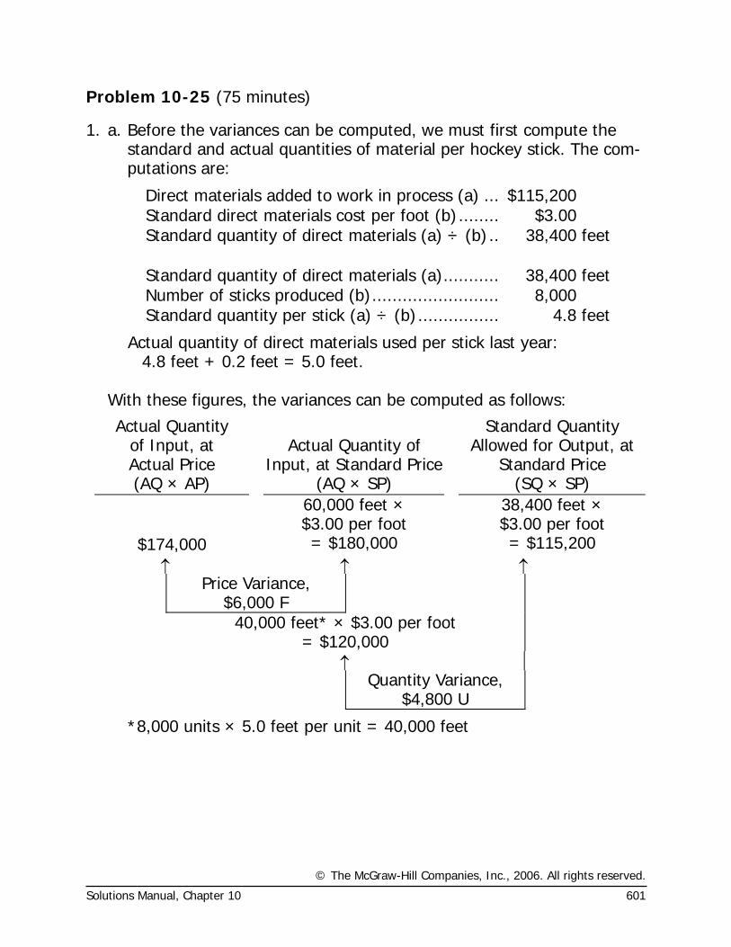
1. a. Before the variances can be computed, we must first compute the standard and actual quantities of material per hockey stick. The com-putations are:
Direct materials added to work in process (a) ... $115,200 Standard direct materials cost per foot (b)........ $3.00 Standard quantity of direct materials (a) ÷ (b).. 38,400 feet Standard quantity of direct materials (a)........... 38,400 feet Number of sticks produced (b)......................... 8,000 Standard quantity per stick (a) ÷ (b)................ 4.8 feet
Actual quantity of direct materials used per stick last year: 4.8 feet + 0.2 feet = 5.0 feet. With these figures, the variances can be computed as follows:
Actual Quantity of Input, at Actual Price
Actual Quantity of
Input, at Standard Price
Standard Quantity Allowed for Output, at
Standard Price (AQ × AP) (AQ × SP) (SQ × SP)
60,000 feet × $3.00 per foot
38,400 feet × $3.00 per foot
$174,000 = $180,000 = $115,200 ↑ ↑ ↑
Price Variance, $6,000 F
40,000 feet* × $3.00 per foot = $120,000
↑ Quantity Variance,
$4,800 U
*8,000 units × 5.0 feet per unit = 40,000 feet
© The McGraw-Hill Companies, Inc., 2006. All rights reserved.
602 Managerial Accounting, 11th Edition
Problem 10-25 (continued)
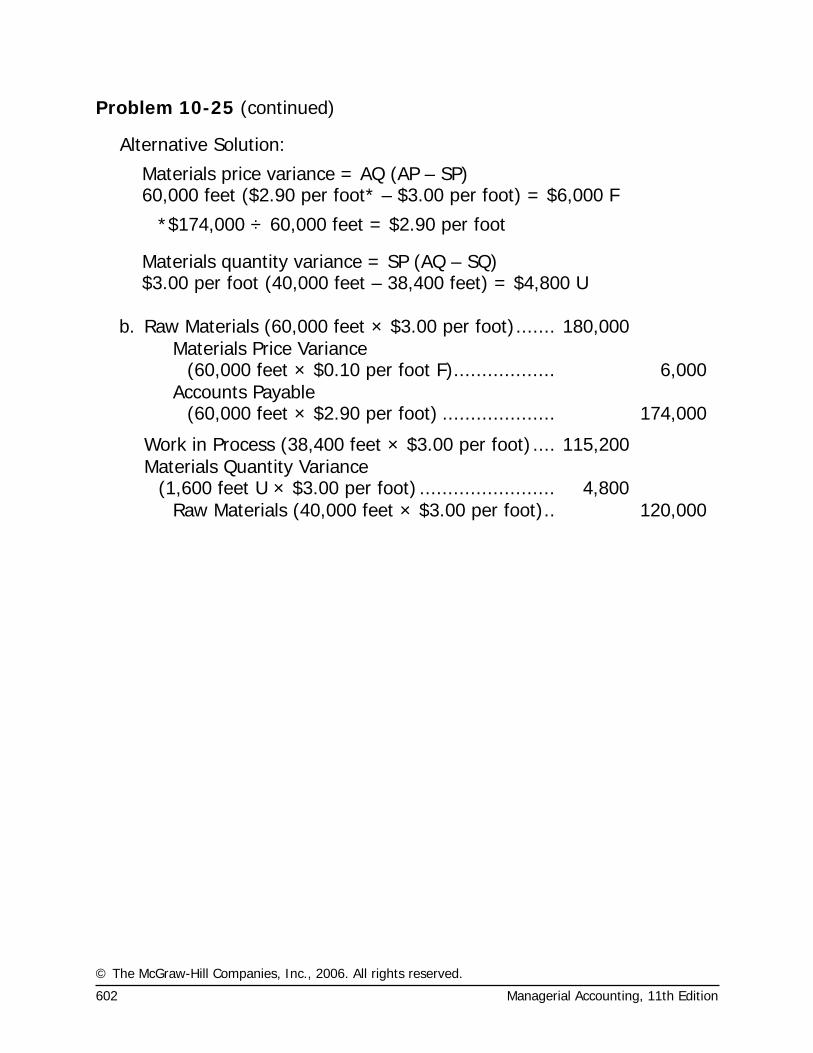
Alternative Solution:
Materials price variance = AQ (AP – SP) 60,000 feet ($2.90 per foot* – $3.00 per foot) = $6,000 F
*$174,000 ÷ 60,000 feet = $2.90 per foot
Materials quantity variance = SP (AQ – SQ) $3.00 per foot (40,000 feet – 38,400 feet) = $4,800 U
b. Raw Materials (60,000 feet × $3.00 per foot)....... 180,000
Materials Price Variance
(60,000 feet × $0.10 per foot F).................. 6,000
Accounts Payable
(60,000 feet × $2.90 per foot) .................... 174,000
Work in Process (38,400 feet × $3.00 per foot).... 115,200
Materials Quantity Variance
(1,600 feet U × $3.00 per foot) ........................ 4,800 Raw Materials (40,000 feet × $3.00 per foot).. 120,000
© The McGraw-Hill Companies, Inc., 2006. All rights reserved.
Solutions Manual, Chapter 10 603
Problem 10-25 (continued)
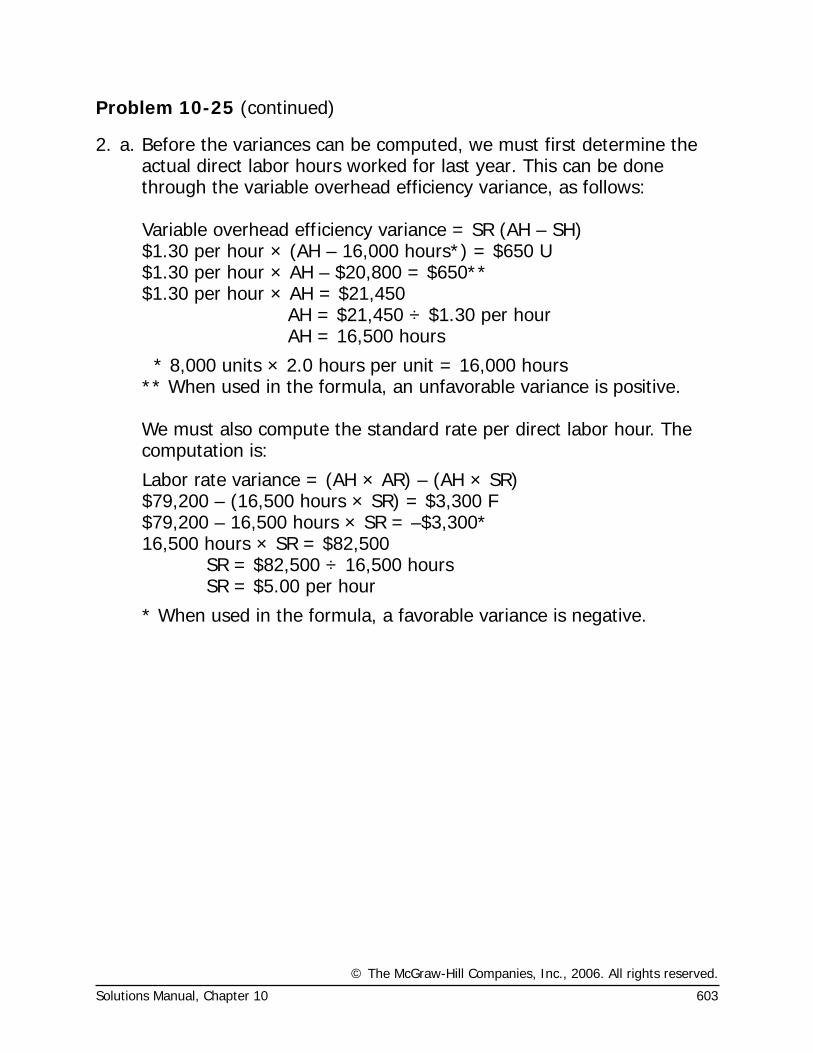
2. a. Before the variances can be computed, we must first determine the actual direct labor hours worked for last year. This can be done through the variable overhead efficiency variance, as follows:
Variable overhead efficiency variance = SR (AH – SH) $1.30 per hour × (AH – 16,000 hours*) = $650 U $1.30 per hour × AH – $20,800 = $650** $1.30 per hour × AH = $21,450 AH = $21,450 ÷ $1.30 per hour AH = 16,500 hours
* 8,000 units × 2.0 hours per unit = 16,000 hours ** When used in the formula, an unfavorable variance is positive. We must also compute the standard rate per direct labor hour. The
computation is:
Labor rate variance = (AH × AR) – (AH × SR) $79,200 – (16,500 hours × SR) = $3,300 F $79,200 – 16,500 hours × SR = –$3,300* 16,500 hours × SR = $82,500 SR = $82,500 ÷ 16,500 hours SR = $5.00 per hour
* When used in the formula, a favorable variance is negative.
© The McGraw-Hill Companies, Inc., 2006. All rights reserved.
604 Managerial Accounting, 11th Edition
Problem 10-25 (continued)
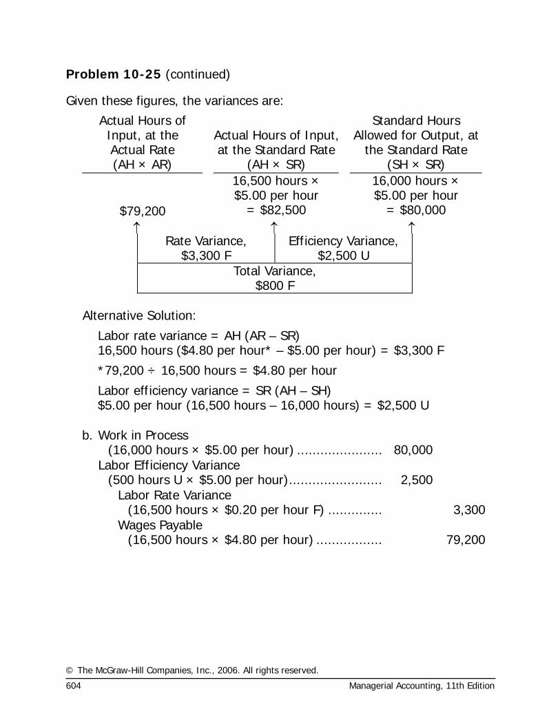
Given these figures, the variances are:
Actual Hours of Input, at the Actual Rate
Actual Hours of Input, at the Standard Rate
Standard Hours Allowed for Output, at
the Standard Rate (AH × AR) (AH × SR) (SH × SR) 16,500 hours ×
$5.00 per hour 16,000 hours ×
$5.00 per hour $79,200 = $82,500 = $80,000 ↑ ↑ ↑
Rate Variance, $3,300 F
Efficiency Variance, $2,500 U
Total Variance, $800 F
Alternative Solution:
Labor rate variance = AH (AR – SR) 16,500 hours ($4.80 per hour* – $5.00 per hour) = $3,300 F
*79,200 ÷ 16,500 hours = $4.80 per hour
Labor efficiency variance = SR (AH – SH) $5.00 per hour (16,500 hours – 16,000 hours) = $2,500 U
b. Work in Process (16,000 hours × $5.00 per hour) ...................... 80,000
Labor Efficiency Variance
(500 hours U × $5.00 per hour)........................ 2,500
Labor Rate Variance
(16,500 hours × $0.20 per hour F) .............. 3,300
Wages Payable
(16,500 hours × $4.80 per hour) ................. 79,200
© The McGraw-Hill Companies, Inc., 2006. All rights reserved.
Solutions Manual, Chapter 10 605
Problem 10-25 (continued)
3. Actual Hours of Input, at the Actual Rate
Actual Hours of Input, at the Standard Rate
Standard Hours Allowed for Output, at
the Standard Rate (AH × AR) (AH × SR) (SH × SR) 16,500 hours ×
$1.30 per hour 16,000 hours ×
$1.30 per hour $19,800 = $21,450 = $20,800 ↑ ↑ ↑
Spending Variance, $1,650 F
Efficiency Variance, $650 U
Total Variance, $1,000 F
Alternative Solution:
Variable overhead spending variance = AH (AR – SR) 16,500 hours ($1.20 per hour* – $1.30 per hour) = $1,650 F
*$19,800 ÷ 16,500 hours = $1.20 per hour
Variable overhead efficiency variance = SR (AH – SH) $1.30 per hour (16,500 hours – 16,000 hours) = $650 U
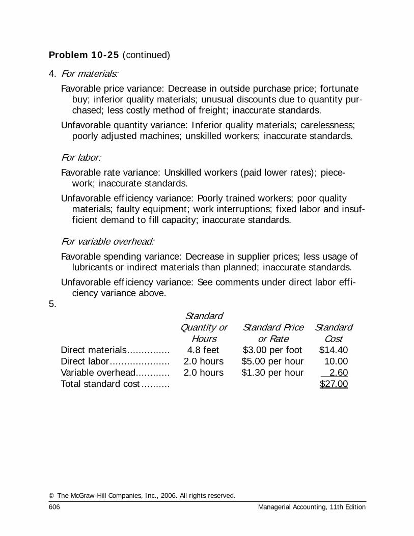
© The McGraw-Hill Companies, Inc., 2006. All rights reserved.
606 Managerial Accounting, 11th Edition
Problem 10-25 (continued)
4. For materials:
Favorable price variance: Decrease in outside purchase price; fortunate buy; inferior quality materials; unusual discounts due to quantity pur-chased; less costly method of freight; inaccurate standards.
Unfavorable quantity variance: Inferior quality materials; carelessness; poorly adjusted machines; unskilled workers; inaccurate standards.
For labor:
Favorable rate variance: Unskilled workers (paid lower rates); piece-work; inaccurate standards.
Unfavorable efficiency variance: Poorly trained workers; poor quality materials; faulty equipment; work interruptions; fixed labor and insuf-ficient demand to fill capacity; inaccurate standards.
For variable overhead:
Favorable spending variance: Decrease in supplier prices; less usage of lubricants or indirect materials than planned; inaccurate standards.
Unfavorable efficiency variance: See comments under direct labor effi-ciency variance above.
5.
Standard Quantity or
Hours Standard Price
or Rate Standard
Cost Direct materials............... 4.8 feet $3.00 per foot $14.40 Direct labor..................... 2.0 hours $5.00 per hour 10.00 Variable overhead............ 2.0 hours $1.30 per hour 2.60 Total standard cost .......... $27.00
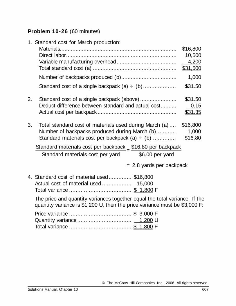
© The McGraw-Hill Companies, Inc., 2006. All rights reserved.
Solutions Manual, Chapter 10 607
Problem 10-26 (60 minutes)
1. Standard cost for March production: Materials.......................................................................... $16,800 Direct labor...................................................................... 10,500 Variable manufacturing overhead...................................... 4,200 Total standard cost (a) ..................................................... $31,500
Number of backpacks produced (b)................................... 1,000
Standard cost of a single backpack (a) ÷ (b).................... $31.50 2. Standard cost of a single backpack (above) ....................... $31.50 Deduct difference between standard and actual cost.......... 0.15 Actual cost per backpack .................................................. $31.35 3. Total standard cost of materials used during March (a) .... $16,800 Number of backpacks produced during March (b)............ 1,000 Standard materials cost per backpack (a) ÷ (b) .............. $16.80
Standard materials cost per backpack $16.80 per backpack=
Standard materials cost per yard $6.00 per yard
= 2.8 yards per backpack
4. Standard cost of material used.............. $16,800 Actual cost of material used .................. 15,000 Total variance ...................................... $ 1,800 F
The price and quantity variances together equal the total variance. If the quantity variance is $1,200 U, then the price variance must be $3,000 F:
Price variance ...................................... $ 3,000 F Quantity variance ................................. 1,200 U Total variance ...................................... $ 1,800 F
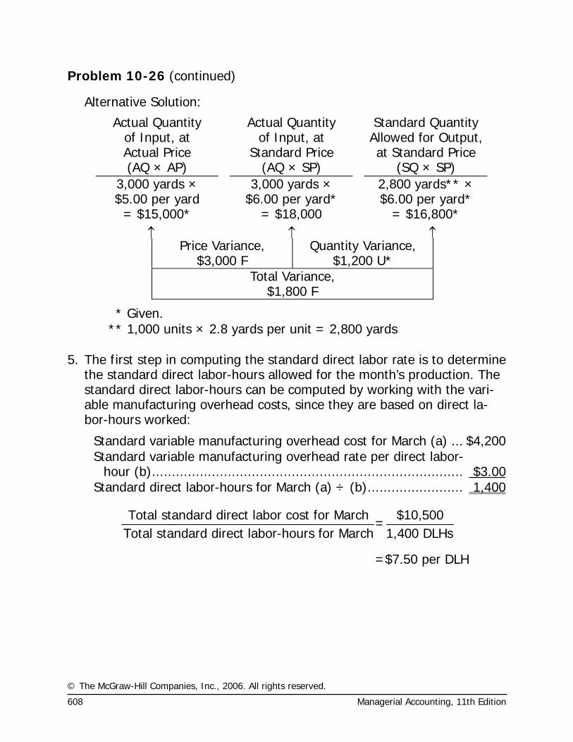
© The McGraw-Hill Companies, Inc., 2006. All rights reserved.
608 Managerial Accounting, 11th Edition
Problem 10-26 (continued)
Alternative Solution:
Actual Quantity of Input, at Actual Price
Actual Quantity of Input, at
Standard Price
Standard Quantity Allowed for Output, at Standard Price
(AQ × AP) (AQ × SP) (SQ × SP) 3,000 yards × $5.00 per yard
3,000 yards × $6.00 per yard*
2,800 yards** × $6.00 per yard*
= $15,000* = $18,000 = $16,800* ↑ ↑ ↑
Price Variance, $3,000 F
Quantity Variance, $1,200 U*
Total Variance, $1,800 F
* Given. ** 1,000 units × 2.8 yards per unit = 2,800 yards
5. The first step in computing the standard direct labor rate is to determine
the standard direct labor-hours allowed for the month’s production. The standard direct labor-hours can be computed by working with the vari-able manufacturing overhead costs, since they are based on direct la-bor-hours worked:
Standard variable manufacturing overhead cost for March (a) ... $4,200Standard variable manufacturing overhead rate per direct labor-
hour (b).............................................................................. $3.00Standard direct labor-hours for March (a) ÷ (b)........................ 1,400
Total standard direct labor cost for March $10,500=
Total standard direct labor-hours for March 1,400 DLHs
=$7.50 per DLH
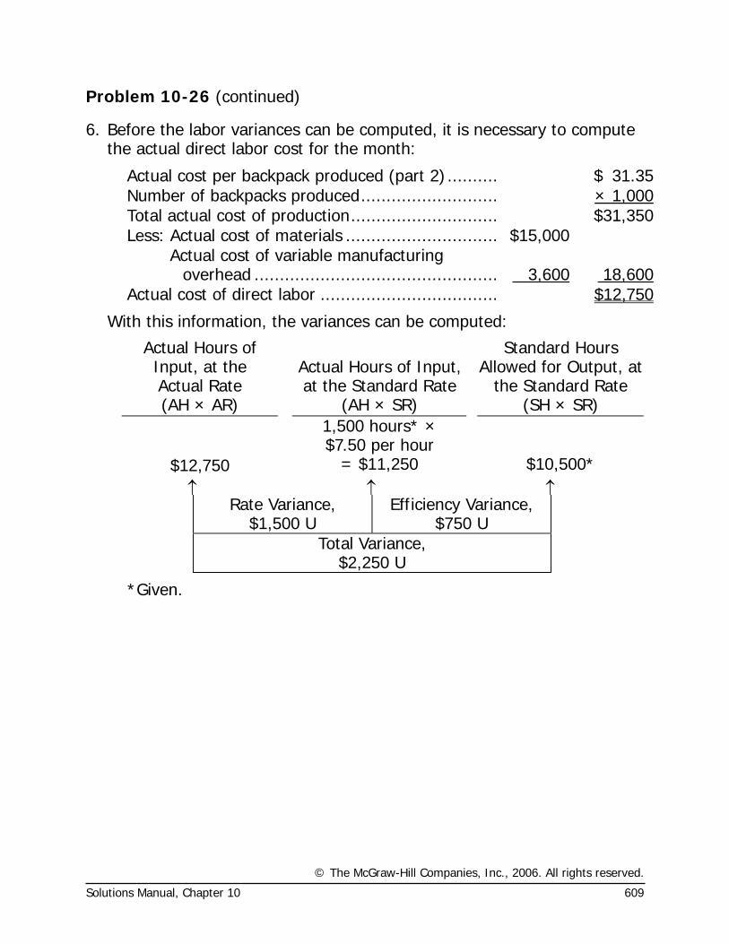
© The McGraw-Hill Companies, Inc., 2006. All rights reserved.
Solutions Manual, Chapter 10 609
Problem 10-26 (continued)
6. Before the labor variances can be computed, it is necessary to compute the actual direct labor cost for the month:
Actual cost per backpack produced (part 2) .......... $ 31.35Number of backpacks produced........................... × 1,000Total actual cost of production............................. $31,350Less: Actual cost of materials .............................. $15,000
Actual cost of variable manufacturing overhead ................................................ 3,600 18,600
Actual cost of direct labor ................................... $12,750
With this information, the variances can be computed:
Actual Hours of Input, at the Actual Rate
Actual Hours of Input, at the Standard Rate
Standard Hours Allowed for Output, at
the Standard Rate (AH × AR) (AH × SR) (SH × SR)
1,500 hours* × $7.50 per hour
$12,750 = $11,250 $10,500* ↑ ↑ ↑
Rate Variance, $1,500 U
Efficiency Variance, $750 U
Total Variance, $2,250 U
*Given.
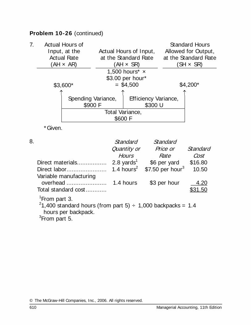
© The McGraw-Hill Companies, Inc., 2006. All rights reserved.
610 Managerial Accounting, 11th Edition
Problem 10-26 (continued)
7. Actual Hours of Input, at the Actual Rate
Actual Hours of Input, at the Standard Rate
Standard Hours Allowed for Output, at the Standard Rate
(AH × AR) (AH × SR) (SH × SR) 1,500 hours* ×
$3.00 per hour*
$3,600* = $4,500 $4,200* ↑ ↑ ↑
Spending Variance, $900 F
Efficiency Variance, $300 U
Total Variance, $600 F
*Given. 8.
Standard Quantity or
Hours
Standard Price or
Rate
Standard
Cost Direct materials................. 2.8 yards1 $6 per yard $16.80 Direct labor....................... 1.4 hours2 $7.50 per hour3 10.50
Variable manufacturing
overhead ....................... 1.4 hours $3 per hour 4.20 Total standard cost............ $31.50
1From part 3. 21,400 standard hours (from part 5) ÷ 1,000 backpacks = 1.4
hours per backpack. 3From part 5.
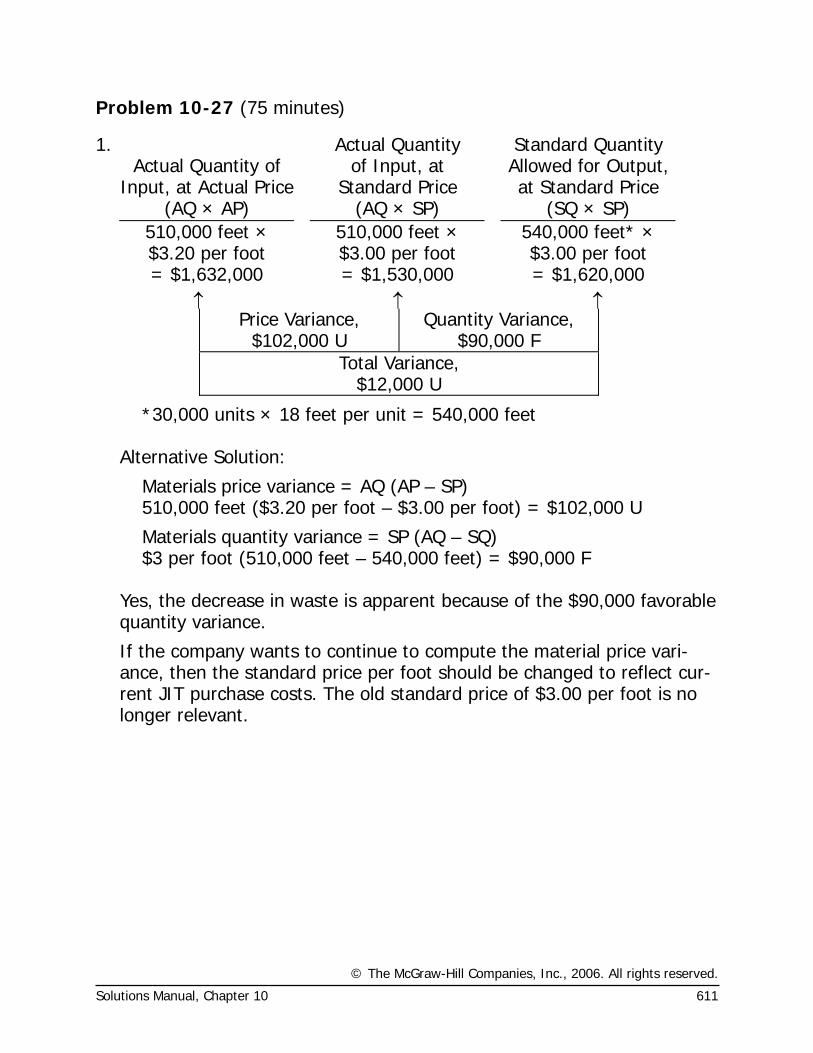
© The McGraw-Hill Companies, Inc., 2006. All rights reserved.
Solutions Manual, Chapter 10 611
Problem 10-27 (75 minutes)
1. Actual Quantity of
Input, at Actual Price
Actual Quantity of Input, at
Standard Price
Standard Quantity Allowed for Output, at Standard Price
(AQ × AP) (AQ × SP) (SQ × SP) 510,000 feet ×
$3.20 per foot 510,000 feet ×
$3.00 per foot 540,000 feet* ×
$3.00 per foot = $1,632,000 = $1,530,000 = $1,620,000 ↑ ↑ ↑
Price Variance, $102,000 U
Quantity Variance, $90,000 F
Total Variance, $12,000 U
*30,000 units × 18 feet per unit = 540,000 feet Alternative Solution:
Materials price variance = AQ (AP – SP) 510,000 feet ($3.20 per foot – $3.00 per foot) = $102,000 U
Materials quantity variance = SP (AQ – SQ) $3 per foot (510,000 feet – 540,000 feet) = $90,000 F Yes, the decrease in waste is apparent because of the $90,000 favorable
quantity variance.
If the company wants to continue to compute the material price vari-ance, then the standard price per foot should be changed to reflect cur-rent JIT purchase costs. The old standard price of $3.00 per foot is no longer relevant.
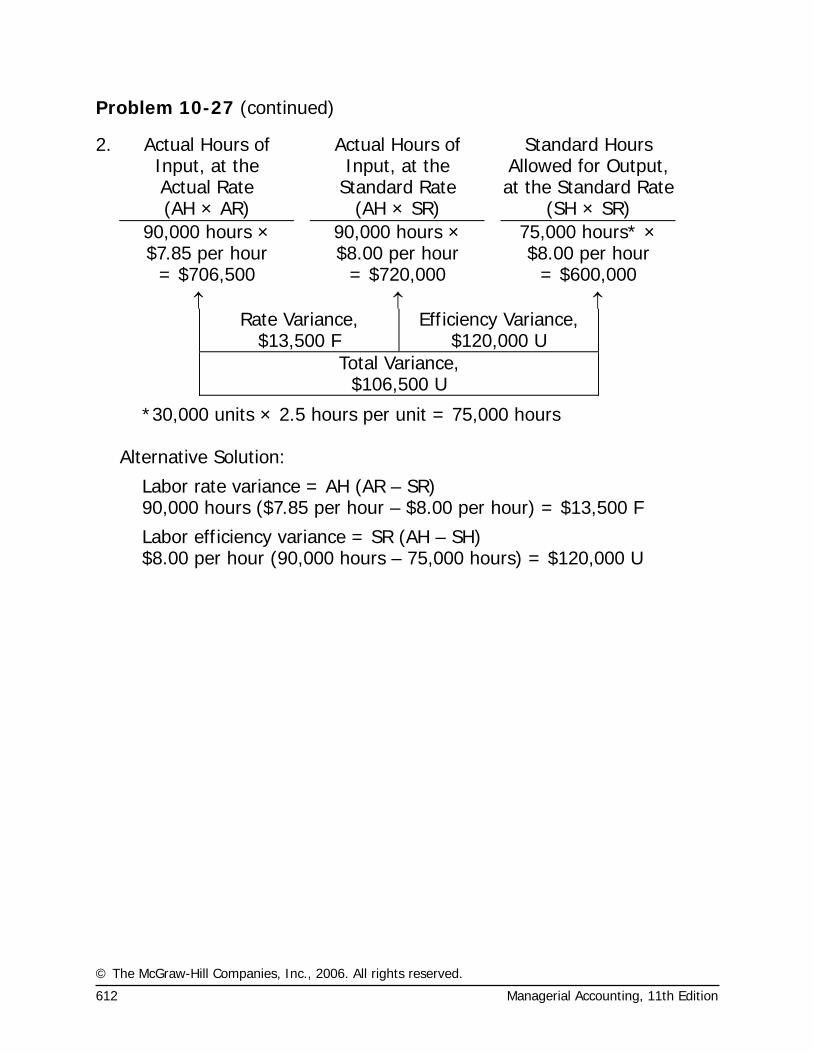
© The McGraw-Hill Companies, Inc., 2006. All rights reserved.
612 Managerial Accounting, 11th Edition
Problem 10-27 (continued)
2. Actual Hours of Input, at the Actual Rate
Actual Hours of Input, at the
Standard Rate
Standard Hours Allowed for Output, at the Standard Rate
(AH × AR) (AH × SR) (SH × SR) 90,000 hours ×
$7.85 per hour 90,000 hours ×
$8.00 per hour 75,000 hours* ×
$8.00 per hour = $706,500 = $720,000 = $600,000 ↑ ↑ ↑
Rate Variance, $13,500 F
Efficiency Variance, $120,000 U
Total Variance, $106,500 U
*30,000 units × 2.5 hours per unit = 75,000 hours Alternative Solution:
Labor rate variance = AH (AR – SR) 90,000 hours ($7.85 per hour – $8.00 per hour) = $13,500 F
Labor efficiency variance = SR (AH – SH) $8.00 per hour (90,000 hours – 75,000 hours) = $120,000 U
© The McGraw-Hill Companies, Inc., 2006. All rights reserved.
Solutions Manual, Chapter 10 613
Problem 10-27 (continued)
No, the labor efficiency variance is not appropriate as a measure of per-formance in this situation. The reasons are:
• Labor is largely a fixed cost rather than a variable cost since the company maintains a stable workforce to operate its flow line. Thus, the variance is not an effective measure of efficiency.
• In a JIT environment the goal is to produce only as needed to meet demand. This often conflicts with the goal of having high labor effi-ciency, which requires that labor be fully utilized producing output. If that output is not really demanded by customers, the result of fully utilizing labor is a buildup of excess work in process and finished goods inventories. This is anathema in a JIT environment. Unfortu-nately, the situation posed in the problem is a common one as com-panies switch from a traditional system to JIT, and sometimes JIT doesn’t work because of misplaced emphasis on efficiency variances. In a JIT setting, it is an interesting paradox that one of the “costs” of greater efficiency on the production line is greater “inefficiency” on the part of labor as it is occasionally idle or as it spends time at vari-ous tasks other than producing goods.
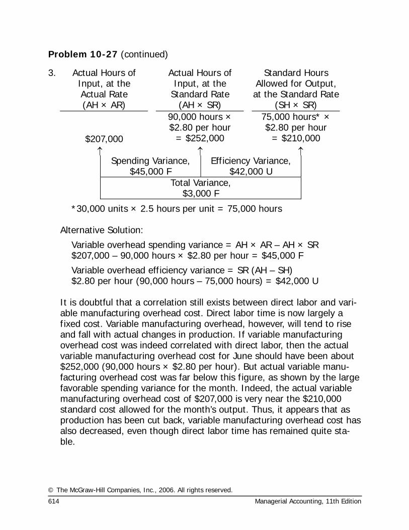
© The McGraw-Hill Companies, Inc., 2006. All rights reserved.
614 Managerial Accounting, 11th Edition
Problem 10-27 (continued)
3. Actual Hours of Input, at the Actual Rate
Actual Hours of Input, at the
Standard Rate
Standard Hours Allowed for Output, at the Standard Rate
(AH × AR) (AH × SR) (SH × SR) 90,000 hours ×
$2.80 per hour 75,000 hours* ×
$2.80 per hour $207,000 = $252,000 = $210,000 ↑ ↑ ↑
Spending Variance, $45,000 F
Efficiency Variance, $42,000 U
Total Variance, $3,000 F
*30,000 units × 2.5 hours per unit = 75,000 hours Alternative Solution:
Variable overhead spending variance = AH × AR – AH × SR $207,000 – 90,000 hours × $2.80 per hour = $45,000 F
Variable overhead efficiency variance = SR (AH – SH) $2.80 per hour (90,000 hours – 75,000 hours) = $42,000 U It is doubtful that a correlation still exists between direct labor and vari-
able manufacturing overhead cost. Direct labor time is now largely a fixed cost. Variable manufacturing overhead, however, will tend to rise and fall with actual changes in production. If variable manufacturing overhead cost was indeed correlated with direct labor, then the actual variable manufacturing overhead cost for June should have been about $252,000 (90,000 hours × $2.80 per hour). But actual variable manu-facturing overhead cost was far below this figure, as shown by the large favorable spending variance for the month. Indeed, the actual variable manufacturing overhead cost of $207,000 is very near the $210,000 standard cost allowed for the month’s output. Thus, it appears that as production has been cut back, variable manufacturing overhead cost has also decreased, even though direct labor time has remained quite sta-ble.
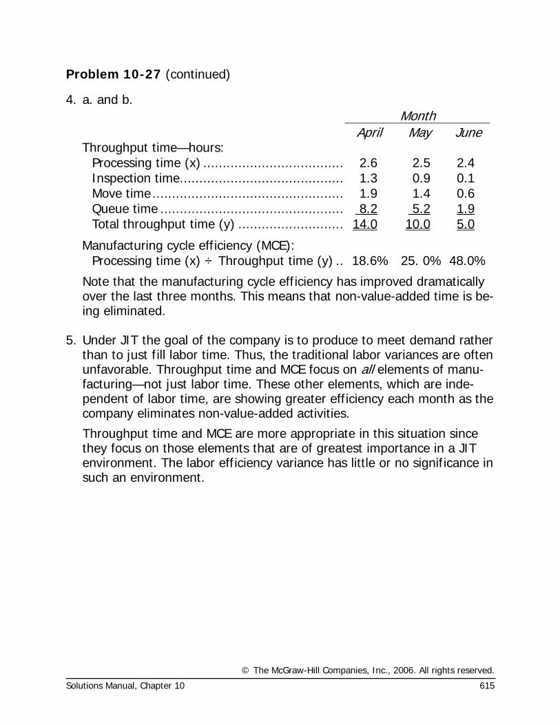
© The McGraw-Hill Companies, Inc., 2006. All rights reserved.
Solutions Manual, Chapter 10 615
Problem 10-27 (continued)
4. a. and b. Month April May June
Throughput time—hours: Processing time (x) ..................................... 2.6 2.5 2.4 Inspection time........................................... 1.3 0.9 0.1 Move time.................................................. 1.9 1.4 0.6 Queue time ................................................ 8.2 5.2 1.9 Total throughput time (y) ............................ 14.0 10.0 5.0
Manufacturing cycle efficiency (MCE): Processing time (x) ÷ Throughput time (y) ... 18.6% 25. 0% 48.0%
Note that the manufacturing cycle efficiency has improved dramatically over the last three months. This means that non-value-added time is be-ing eliminated.
5. Under JIT the goal of the company is to produce to meet demand rather
than to just fill labor time. Thus, the traditional labor variances are often unfavorable. Throughput time and MCE focus on all elements of manu-facturing—not just labor time. These other elements, which are inde-pendent of labor time, are showing greater efficiency each month as the company eliminates non-value-added activities.
Throughput time and MCE are more appropriate in this situation since they focus on those elements that are of greatest importance in a JIT environment. The labor efficiency variance has little or no significance in such an environment.
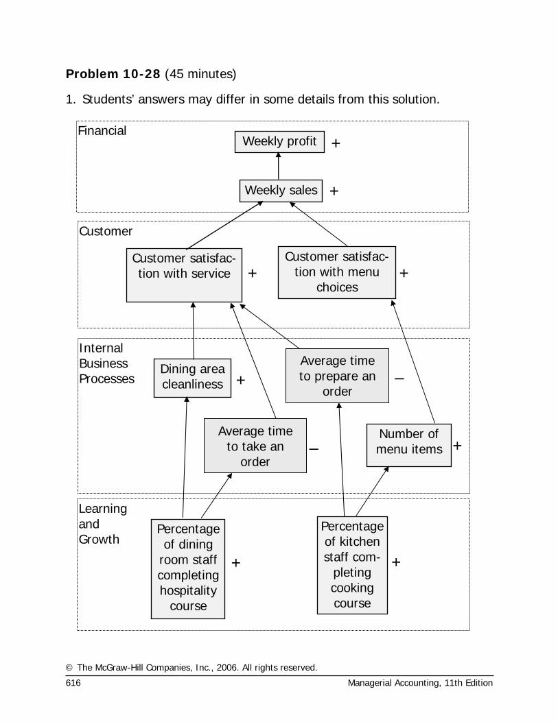
© The McGraw-Hill Companies, Inc., 2006. All rights reserved.
616 Managerial Accounting, 11th Edition
Learning and Growth
Internal Business Processes
Financial
Customer
Problem 10-28 (45 minutes)
1. Students’ answers may differ in some details from this solution.
Weekly profit
Weekly sales
Number of menu items
Dining area cleanliness
Percentage of kitchen staff com-
pleting cooking course
+
+
+
+
Customer satisfac-tion with service
Customer satisfac-tion with menu
choices + +
Average time to prepare an
order
Average time to take an
order
Percentage of dining
room staff completing hospitality
course
+
+ –
–
© The McGraw-Hill Companies, Inc., 2006. All rights reserved.
Solutions Manual, Chapter 10 617
Problem 10-28 (continued)
2. The hypotheses underlying the balanced scorecard are indicated by the arrows in the diagram. Reading from the bottom of the balanced score-card, the hypotheses are: o If the percentage of dining room staff who complete the basic hospi-
tality course increases, then the average time to take an order will decrease.
o If the percentage of dining room staff who complete the basic hospi-tality course increases, then dining room cleanliness will improve.
o If the percentage of kitchen staff who complete the basic cooking course increases, then the average time to prepare an order will de-crease.
o If the percentage of kitchen staff who complete the basic cooking course increases, then the number of menu items will increase.
o If the dining room cleanliness improves, then customer satisfaction with service will increase.
o If the average time to take an order decreases, then customer satis-faction with service will increase.
o If the average time to prepare an order decreases, then customer satisfaction with service will increase.
o If the number of menu items increases, then customer satisfaction with menu choices will increase.
o If customer satisfaction with service increases, weekly sales will in-crease.
o If customer satisfaction with menu choices increases, weekly sales will increase.
o If sales increase, weekly profits for the Lodge will increase.
Each of these hypotheses is questionable to some degree. For example, the items added to the menu may not appeal to customers. So even if the number of menu items increases, customer satisfaction with the menu choices may not increase. The fact that each of the hypotheses can be questioned does not, however, invalidate the balanced score-card. If the scorecard is used correctly, management will be able to identify which, if any, of the hypotheses are incorrect. [See below.]
© The McGraw-Hill Companies, Inc., 2006. All rights reserved.
618 Managerial Accounting, 11th Edition
Problem 10-28 (continued)
3. Management will be able to tell if a hypothesis is false if an improve-ment in a performance measure at the bottom of an arrow does not, in fact, lead to improvement in the performance measure at the tip of the arrow. For example, if the number of menu items is increased, but cus-tomer satisfaction with the menu choices does not increase, manage-ment will immediately know that something was wrong with that par-ticular hypothesis.
© The McGraw-Hill Companies, Inc., 2006. All rights reserved.
Solutions Manual, Chapter 10 619
Problem 10-29 (45 minutes)
The answers below are not the only possible answers. Ingenious people can figure out many different ways of making performance look better even though it really isn’t. This is one of the reasons for a balanced score-card. By having a number of different measures that ultimately are linked to overall financial goals, “gaming” the system is more difficult. 1. Speed-to-market can be improved by taking on less ambitious projects.
Instead of working on major product innovations that require a great deal of time and effort, R&D may choose to work on small, incremental improvements in existing products. There is also a danger that in the rush to push products out the door, the products will be inadequately tested and developed.
2. Performance measures that are ratios or percentages present special
dangers. A ratio can be increased either by increasing the numerator or by decreasing the denominator. Usually, the intention is to increase the numerator in the ratio, but a manager may react by decreasing the de-nominator instead. In this case (which actually happened), the manag-ers pulled telephones out of the high-crime areas. This eliminated the problem for the managers, but was not what the CEO or the city offi-cials had intended. They wanted the phones fixed, not eliminated.
3. In real life, the production manager simply added several weeks to the
delivery cycle time. In other words, instead of promising to deliver an order in four weeks, the manager promised to deliver in six weeks. This increase in delivery cycle time did not, of course, please customers and drove some business away, but it dramatically improved the percentage of orders delivered on time.
© The McGraw-Hill Companies, Inc., 2006. All rights reserved.
620 Managerial Accounting, 11th Edition
Problem 10-29 (continued)
4. As stated above, ratios can be improved by changing either the numera-tor or the denominator. Managers who are under pressure to increase the revenue per employee may find it easier to eliminate employees than to increase revenues. Of course, eliminating employees may reduce total revenues and total profits, but the revenue per employee will in-crease as long as the percentage decline in revenues is less than the percentage cut in number of employees. Suppose, for example, that a manager is responsible for business units with a total of 1,000 employ-ees, $120 million in revenues, and profits of $2 million. Further suppose that a manager can eliminate one of these business units that has 200 employees, revenues of $10 million, and profits of $1.2 million.
Before eliminating the business unit
After eliminating the business unit
Total revenue ................ $120,000,000 $110,000,000 Total employees............. 1,000 800 Revenue per employee ... $120,000 $137,500 Total profits................... $2,000,000 $800,000
As these examples illustrate, performance measures should be selected
with a great deal of care and managers should avoid placing too much emphasis on any one performance measure.
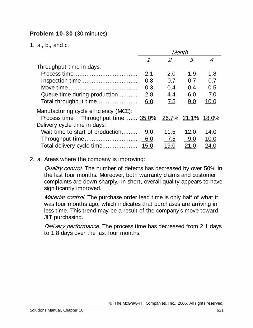
© The McGraw-Hill Companies, Inc., 2006. All rights reserved.
Solutions Manual, Chapter 10 621
Problem 10-30 (30 minutes)
1. a., b., and c. Month
1 2 3 4 Throughput time in days:
Process time.................................... 2.1 2.0 1.9 1.8 Inspection time................................ 0.8 0.7 0.7 0.7 Move time ....................................... 0.3 0.4 0.4 0.5 Queue time during production........... 2.8 4.4 6.0 7.0 Total throughput time....................... 6.0 7.5 9.0 10.0
Manufacturing cycle efficiency (MCE): Process time ÷ Throughput time ....... 35.0% 26.7% 21.1% 18.0%
Delivery cycle time in days: Wait time to start of production......... 9.0 11.5 12.0 14.0 Throughput time.............................. 6.0 7.5 9.0 10.0 Total delivery cycle time.................... 15.0 19.0 21.0 24.0
2. a. Areas where the company is improving:
Quality control. The number of defects has decreased by over 50% in the last four months. Moreover, both warranty claims and customer complaints are down sharply. In short, overall quality appears to have significantly improved.
Material control. The purchase order lead time is only half of what it was four months ago, which indicates that purchases are arriving in less time. This trend may be a result of the company’s move toward JIT purchasing.
Delivery performance. The process time has decreased from 2.1 days to 1.8 days over the last four months.
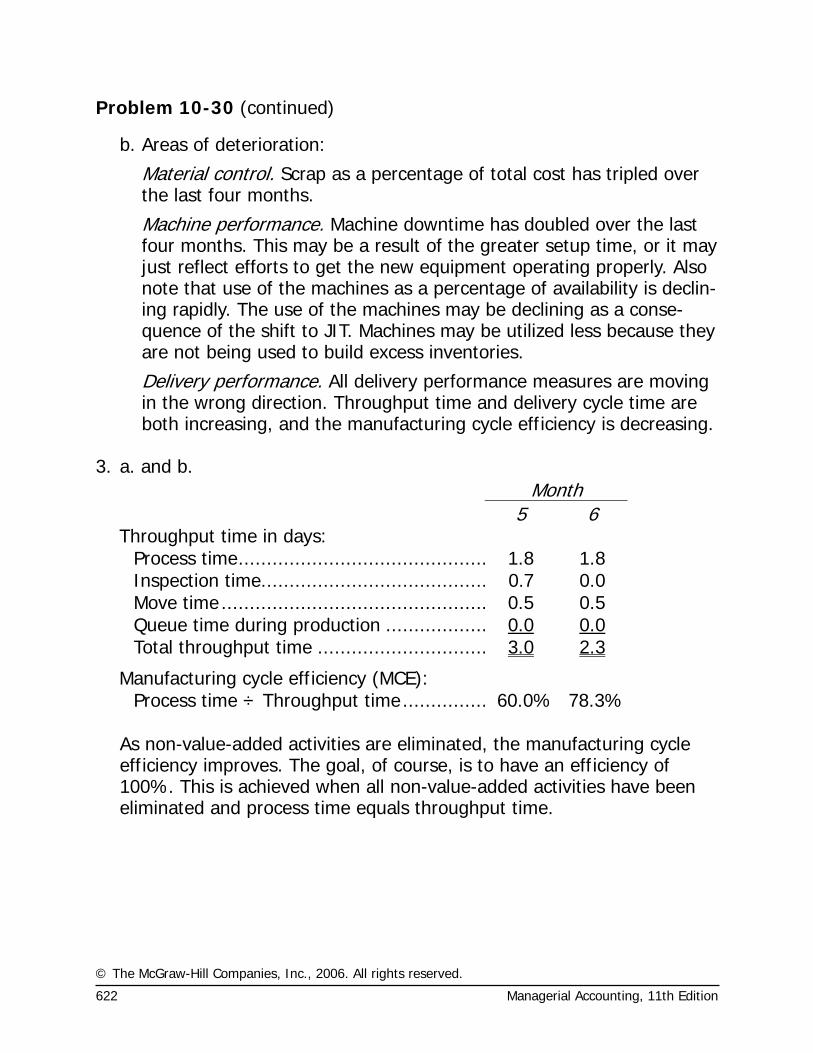
© The McGraw-Hill Companies, Inc., 2006. All rights reserved.
622 Managerial Accounting, 11th Edition
Problem 10-30 (continued)
b. Areas of deterioration:
Material control. Scrap as a percentage of total cost has tripled over the last four months.
Machine performance. Machine downtime has doubled over the last four months. This may be a result of the greater setup time, or it may just reflect efforts to get the new equipment operating properly. Also note that use of the machines as a percentage of availability is declin-ing rapidly. The use of the machines may be declining as a conse-quence of the shift to JIT. Machines may be utilized less because they are not being used to build excess inventories.
Delivery performance. All delivery performance measures are moving in the wrong direction. Throughput time and delivery cycle time are both increasing, and the manufacturing cycle efficiency is decreasing.
3. a. and b.
Month 5 6 Throughput time in days:
Process time............................................ 1.8 1.8 Inspection time........................................ 0.7 0.0 Move time............................................... 0.5 0.5 Queue time during production .................. 0.0 0.0 Total throughput time .............................. 3.0 2.3
Manufacturing cycle efficiency (MCE): Process time ÷ Throughput time............... 60.0% 78.3%
As non-value-added activities are eliminated, the manufacturing cycle
efficiency improves. The goal, of course, is to have an efficiency of 100%. This is achieved when all non-value-added activities have been eliminated and process time equals throughput time.
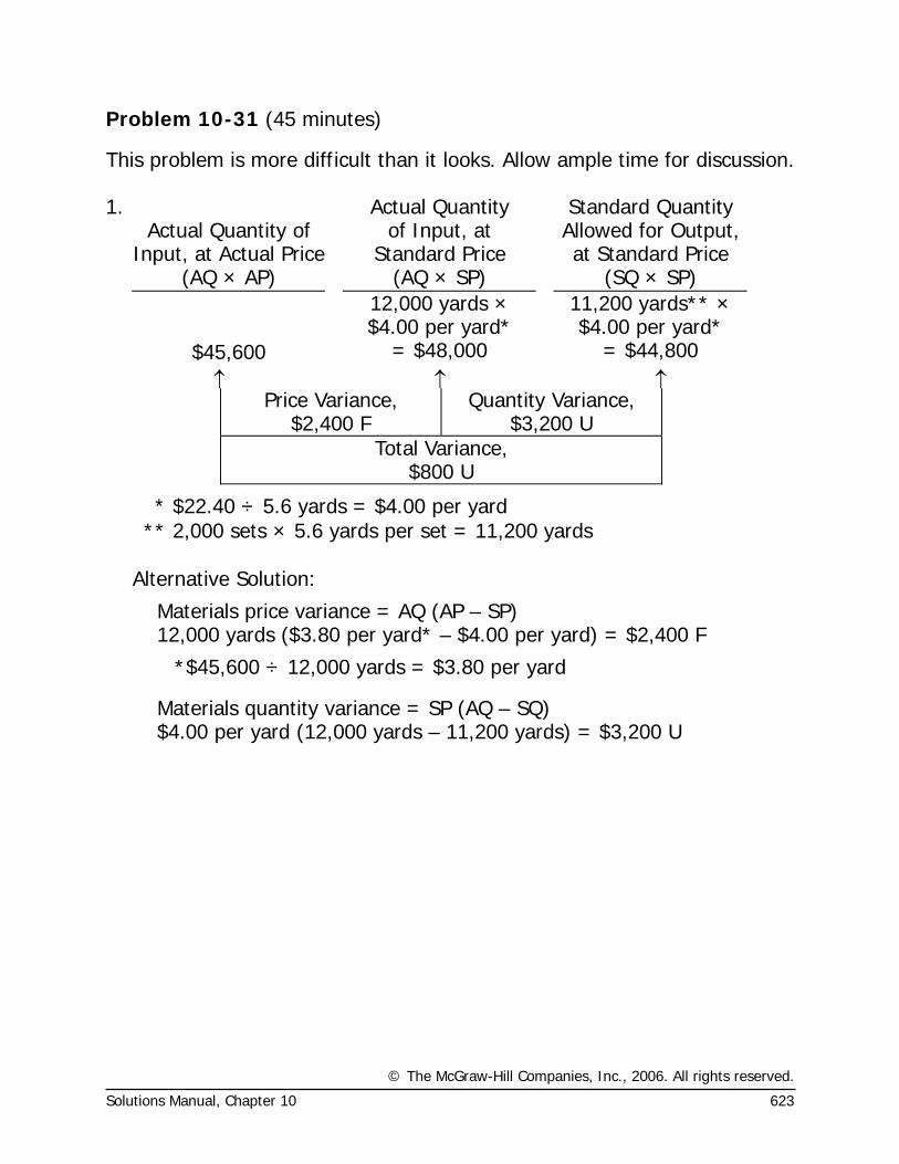
© The McGraw-Hill Companies, Inc., 2006. All rights reserved.
Solutions Manual, Chapter 10 623
Problem 10-31 (45 minutes)
This problem is more difficult than it looks. Allow ample time for discussion. 1.
Actual Quantity of Input, at Actual Price
Actual Quantity of Input, at
Standard Price
Standard Quantity Allowed for Output, at Standard Price
(AQ × AP) (AQ × SP) (SQ × SP) 12,000 yards ×
$4.00 per yard* 11,200 yards** ×
$4.00 per yard* $45,600 = $48,000 = $44,800 ↑ ↑ ↑
Price Variance, $2,400 F
Quantity Variance, $3,200 U
Total Variance, $800 U
* $22.40 ÷ 5.6 yards = $4.00 per yard ** 2,000 sets × 5.6 yards per set = 11,200 yards
Alternative Solution:
Materials price variance = AQ (AP – SP) 12,000 yards ($3.80 per yard* – $4.00 per yard) = $2,400 F
*$45,600 ÷ 12,000 yards = $3.80 per yard
Materials quantity variance = SP (AQ – SQ) $4.00 per yard (12,000 yards – 11,200 yards) = $3,200 U
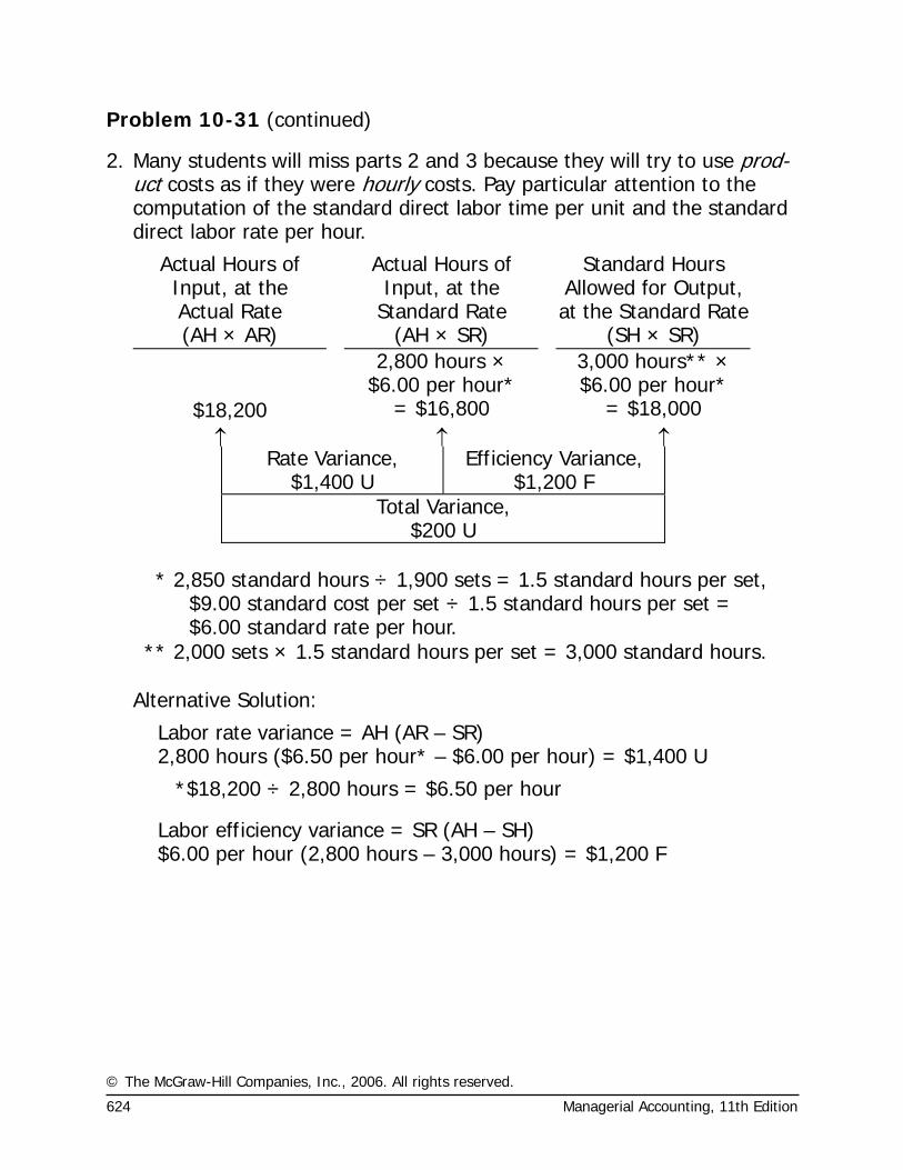
© The McGraw-Hill Companies, Inc., 2006. All rights reserved.
624 Managerial Accounting, 11th Edition
Problem 10-31 (continued)
2. Many students will miss parts 2 and 3 because they will try to use prod-uct costs as if they were hourly costs. Pay particular attention to the computation of the standard direct labor time per unit and the standard direct labor rate per hour.
Actual Hours of Input, at the Actual Rate
Actual Hours of Input, at the
Standard Rate
Standard Hours Allowed for Output, at the Standard Rate
(AH × AR) (AH × SR) (SH × SR) 2,800 hours ×
$6.00 per hour* 3,000 hours** ×
$6.00 per hour* $18,200 = $16,800 = $18,000
↑ ↑ ↑ Rate Variance,
$1,400 U Efficiency Variance,
$1,200 F Total Variance,
$200 U
* 2,850 standard hours ÷ 1,900 sets = 1.5 standard hours per set, $9.00 standard cost per set ÷ 1.5 standard hours per set = $6.00 standard rate per hour.
** 2,000 sets × 1.5 standard hours per set = 3,000 standard hours. Alternative Solution:
Labor rate variance = AH (AR – SR) 2,800 hours ($6.50 per hour* – $6.00 per hour) = $1,400 U
*$18,200 ÷ 2,800 hours = $6.50 per hour
Labor efficiency variance = SR (AH – SH) $6.00 per hour (2,800 hours – 3,000 hours) = $1,200 F
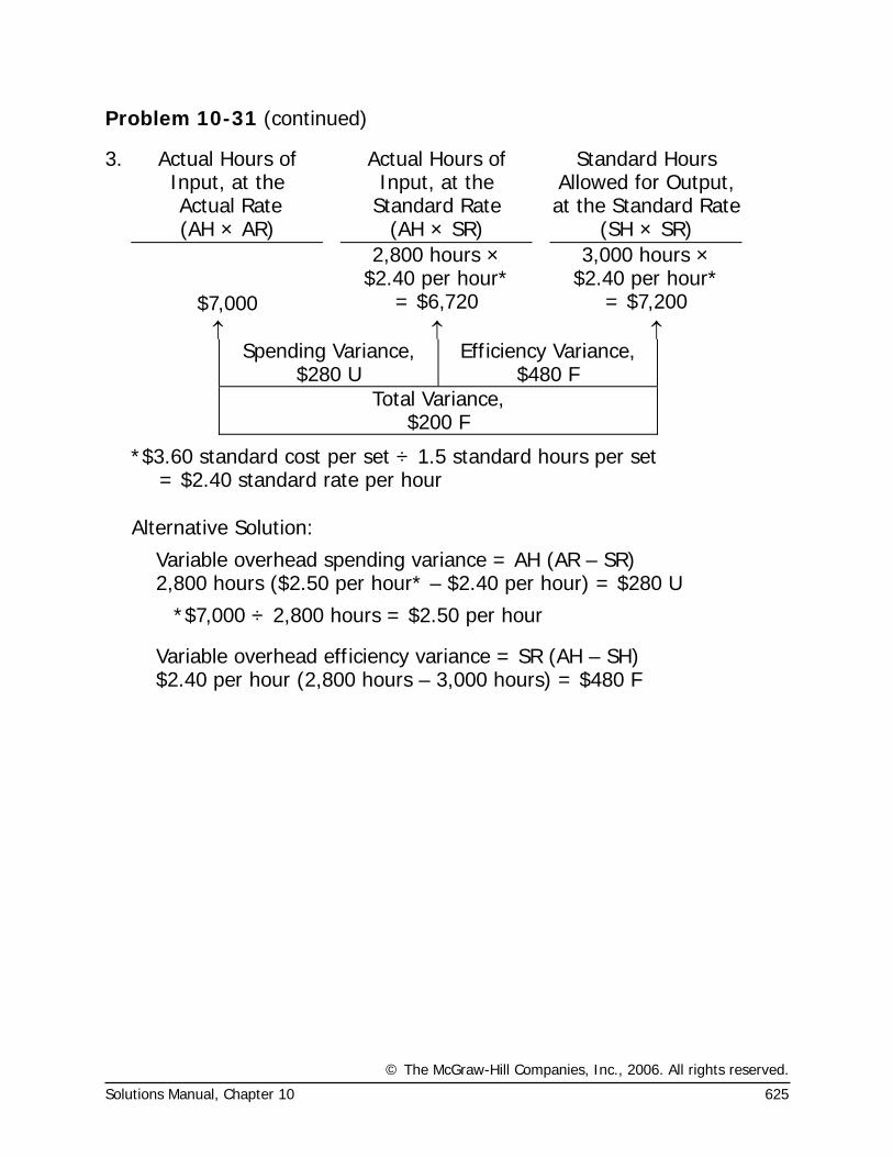
© The McGraw-Hill Companies, Inc., 2006. All rights reserved.
Solutions Manual, Chapter 10 625
Problem 10-31 (continued)
3. Actual Hours of Input, at the Actual Rate
Actual Hours of Input, at the
Standard Rate
Standard Hours Allowed for Output, at the Standard Rate
(AH × AR) (AH × SR) (SH × SR) 2,800 hours ×
$2.40 per hour* 3,000 hours ×
$2.40 per hour* $7,000 = $6,720 = $7,200 ↑ ↑ ↑
Spending Variance, $280 U
Efficiency Variance, $480 F
Total Variance, $200 F
*$3.60 standard cost per set ÷ 1.5 standard hours per set = $2.40 standard rate per hour
Alternative Solution:
Variable overhead spending variance = AH (AR – SR) 2,800 hours ($2.50 per hour* – $2.40 per hour) = $280 U
*$7,000 ÷ 2,800 hours = $2.50 per hour
Variable overhead efficiency variance = SR (AH – SH) $2.40 per hour (2,800 hours – 3,000 hours) = $480 F
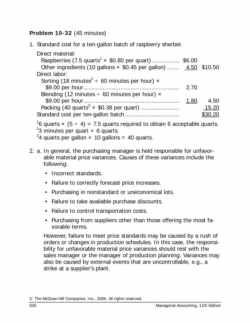
© The McGraw-Hill Companies, Inc., 2006. All rights reserved.
626 Managerial Accounting, 11th Edition
Problem 10-32 (45 minutes)
1. Standard cost for a ten-gallon batch of raspberry sherbet.
Direct material: Raspberries (7.5 quarts1 × $0.80 per quart)................ $6.00 Other ingredients (10 gallons × $0.45 per gallon) ....... 4.50 $10.50
Direct labor: Sorting (18 minutes2 ÷ 60 minutes per hour) ×
$9.00 per hour....................................................... 2.70 Blending (12 minutes ÷ 60 minutes per hour) ×
$9.00 per hour....................................................... 1.80 4.50Packing (40 quarts3 × $0.38 per quart) ...................... 15.20
Standard cost per ten-gallon batch ............................... $30.20
16 quarts × (5 ÷ 4) = 7.5 quarts required to obtain 6 acceptable quarts. 23 minutes per quart × 6 quarts. 34 quarts per gallon × 10 gallons = 40 quarts.
2. a. In general, the purchasing manager is held responsible for unfavor-
able material price variances. Causes of these variances include the following:
• Incorrect standards.
• Failure to correctly forecast price increases.
• Purchasing in nonstandard or uneconomical lots.
• Failure to take available purchase discounts.
• Failure to control transportation costs.
• Purchasing from suppliers other than those offering the most fa-vorable terms.
However, failure to meet price standards may be caused by a rush of orders or changes in production schedules. In this case, the responsi-bility for unfavorable material price variances should rest with the sales manager or the manager of production planning. Variances may also be caused by external events that are uncontrollable, e.g., a strike at a supplier’s plant.
© The McGraw-Hill Companies, Inc., 2006. All rights reserved.
Solutions Manual, Chapter 10 627
Problem 10-32 (continued)
b. In general, the production manager or foreman is held responsible for unfavorable labor efficiency variances. Causes of these variances in-clude the following:
• Incorrect standards.
• Poorly trained labor.
• Substandard or inefficient equipment.
• Inadequate supervision.
• Machine breakdowns from poor maintenance.
• Poorly motivated employees.
• Fixed labor force with demand less than capacity.
Failure to meet labor efficiency standards may also be caused by the use of inferior materials or poor production planning. In these cases, responsibility should rest with the purchasing manager or the man-ager of production planning. Variances may also be caused by exter-nal events that are uncontrollable, e.g., low unemployment leading to the inability to hire and retain skilled workers.
(Unofficial CMA Solution, adapted)
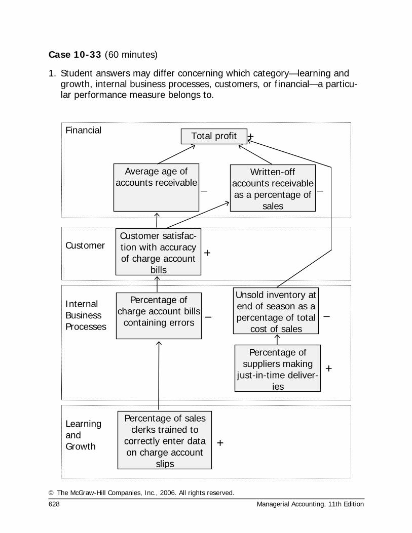
© The McGraw-Hill Companies, Inc., 2006. All rights reserved.
628 Managerial Accounting, 11th Edition
Learning and Growth
Internal Business Processes
Customer
Financial
Case 10-33 (60 minutes)
1. Student answers may differ concerning which category—learning and growth, internal business processes, customers, or financial—a particu-lar performance measure belongs to.
Total profit
Average age of accounts receivable
Written-off accounts receivable as a percentage of
sales
Customer satisfac-tion with accuracy of charge account
bills
Percentage of charge account bills
containing errors
Unsold inventory at end of season as a percentage of total
cost of sales
Percentage of suppliers making
just-in-time deliver-ies
Percentage of sales clerks trained to
correctly enter data on charge account
slips
+
+
+
+
−
− −
−
© The McGraw-Hill Companies, Inc., 2006. All rights reserved.
Solutions Manual, Chapter 10 629
Case 10-33 (continued)
A number of the performance measures suggested by managers have not been included in the above balanced scorecard. The excluded per-formance measures may have an impact on total profit, but they are not linked in any obvious way with the two key problems that have been identified by management—accounts receivables and unsold inventory. If every performance measure that potentially impacts profit is included in a company’s balanced scorecard, it would become unwieldy and focus would be lost.
2. The results of operations can be exploited for information about the
company’s strategy. Each link in the balanced scorecard should be re-garded as a hypothesis of the form “If ..., then ...”. For example, the balanced scorecard on the previous page contains the hypothesis “If customers express greater satisfaction with the accuracy of their charge account bills, then the average age of accounts receivable will improve.” If customers in fact do express greater satisfaction with the accuracy of their charge account bills, but the average age of accounts receivable does not improve, this would have to be considered evidence that is in-consistent with the hypothesis. Management should try to figure out why the average age of receivables has not improved. (See the answer below for possible explanations.) The answer may suggest a shift in strategy.
In general, the most important results are those that provide evidence inconsistent with the hypotheses embedded in the balanced scorecard. Such evidence suggests that the company’s strategy needs to be reex-amined.
© The McGraw-Hill Companies, Inc., 2006. All rights reserved.
630 Managerial Accounting, 11th Edition
Case 10-33 (continued)
3. a. This evidence is inconsistent with two of the hypotheses underlying the balanced scorecard. The first of these hypotheses is “If customers express greater satisfaction with the accuracy of their charge account bills, then the average age of accounts receivable will improve.” The second of these hypotheses is “If customers express greater satisfac-tion with the accuracy of their charge account bills, then there will be improvement in bad debts.” There are a number of possible explana-tions. Two possibilities are that the company’s collection efforts are ineffective and that the company’s credit reviews are not working properly. In other words, the problem may not be incorrect charge account bills at all. The problem may be that the procedures for col-lecting overdue accounts are not working properly. Or, the problem may be that the procedures for reviewing credit card applications let through too many poor credit risks. If so, this would suggest that ef-forts should be shifted from reducing charge account billing errors to improving the internal business processes dealing with collections and credit screening. And in that case, the balanced scorecard should be modified.
b. This evidence is inconsistent with three hypotheses. The first of these
is “If the average age of receivables declines, then profits will in-crease.” The second hypothesis is “If the written-off accounts receiv-able decrease as a percentage of sales, then profits will increase.” The third hypothesis is “If unsold inventory at the end of the season as a percentage of cost of sales declines, then profits will increase.”
Again, there are a number of possible explanations for the lack of re-sults consistent with the hypotheses. Managers may have decreased the average age of receivables by simply writing off old accounts ear-lier than was done previously. This would actually decrease reported profits in the short term. Bad debts as a percentage of sales could be decreased by drastically cutting back on extensions of credit to cus-tomers—perhaps even canceling some charge accounts. (Bad debts would be zero if there were no credit sales.) This would have the ef-fect of reducing bad debts, but might irritate otherwise loyal credit customers and reduce sales and profits.
© The McGraw-Hill Companies, Inc., 2006. All rights reserved.
Solutions Manual, Chapter 10 631
Case 10-33 (continued)
The reduction in unsold inventories at the end of the season as a percentage of cost of sales could have occurred for a number of rea-sons that are not necessarily good for profits. For example, managers may have been too cautious about ordering goods to restock low in-ventories—creating stockouts and lost sales. Or, managers may have cut prices drastically on excess inventories in order to eliminate them before the end of the season. This may have reduced the willingness of customers to pay the store’s normal prices. Or, managers may have gotten rid of excess inventories by selling them to discounters before the end of the season.
© The McGraw-Hill Companies, Inc., 2006. All rights reserved.
632 Managerial Accounting, 11th Edition
Case 10-34 (30 minutes)
This case may be difficult for some students to grasp since it requires look-ing at standard costs from an entirely different perspective. In this case, standard costs have been inappropriately used as a means to manipulate reported earnings rather than as a way to control costs. 1. Lansing has evidently set very loose standards in which the standard
prices and standard quantities are far too high. This guarantees that fa-vorable variances will ordinarily result from operations. If the standard costs are set artificially high, the standard cost of goods sold will be arti-ficially high and thus the division’s net operating income will be de-pressed until the favorable variances are recognized. If Lansing saves the favorable variances, he can release just enough in the second and third quarters to show some improvement and then he can release all of the rest in the last quarter, creating the annual “Christmas present.”
2. Lansing should not be permitted to continue this practice for several
reasons. First, it distorts the quarterly earnings for both the division and the company. The distortions of the division’s quarterly earnings are troubling because the manipulations may mask real signs of trouble. The distortions of the company’s quarterly earnings are troubling because they may mislead external users of the financial statements. Second, Lansing should not be rewarded for manipulating earnings. This sets a moral tone in the company that is likely to lead to even deeper trouble. Indeed, the permissive attitude of top management toward the manipu-lation of earnings may indicate the existence of other, even more seri-ous, ethical problems in the company. Third, a clear message should be sent to division managers like Lansing that their job is to manage their operations, not their earnings. If they keep on top of operations and manage well, the earnings should take care of themselves.
© The McGraw-Hill Companies, Inc., 2006. All rights reserved.
Solutions Manual, Chapter 10 633
Case 10-34 (continued)
3. Stacy Cummins does not have any easy alternatives available. She has already taken the problem to the President, who was not interested. If she goes around the President to the Board of Directors, she will be put-ting herself in a politically difficult position with little likelihood that it will do much good if, in fact, the Board of Directors already knows what is going on.
On the other hand, if she simply goes along, she will be violating the “Objectivity” standard of ethical conduct for management accountants. The Home Security Division’s manipulation of quarterly earnings does distort the entire company’s quarterly reports. And the Objectivity stan-dard clearly stipulates that “management accountants have a responsi-bility to disclose fully all relevant information that could reasonably be expected to influence an intended user’s understanding of the reports, comments, and recommendations presented.” Apart from the ethical is-sue, there is also a very practical consideration. If Merced Home Prod-ucts becomes embroiled in controversy concerning questionable ac-counting practices, Stacy Cummins will be viewed as a responsible party by outsiders and her career is likely to suffer dramatically and she may even face legal problems.
We would suggest that Ms. Cummins quietly bring the manipulation of earnings to the attention of the audit committee of the Board of Direc-tors, carefully laying out in a non-confrontational manner the problems created by Lansing’s practice of manipulating earnings. If the President and the Board of Directors are still not interested in dealing with the problem, she may reasonably conclude that the best alternative is to start looking for another job.
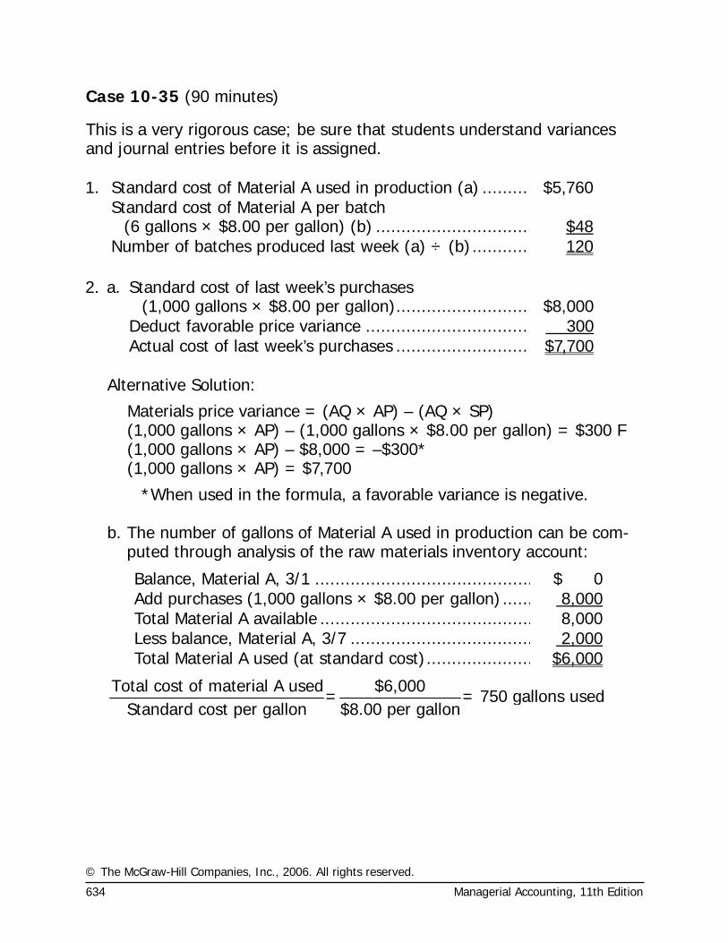
© The McGraw-Hill Companies, Inc., 2006. All rights reserved.
634 Managerial Accounting, 11th Edition
Case 10-35 (90 minutes)
This is a very rigorous case; be sure that students understand variances and journal entries before it is assigned. 1. Standard cost of Material A used in production (a) .......... $5,760
Standard cost of Material A per batch
(6 gallons × $8.00 per gallon) (b) ............................... $48 Number of batches produced last week (a) ÷ (b)............ 120 2. a. Standard cost of last week’s purchases
(1,000 gallons × $8.00 per gallon)........................... $8,000 Deduct favorable price variance ................................. 300 Actual cost of last week’s purchases ........................... $7,700 Alternative Solution:
Materials price variance = (AQ × AP) – (AQ × SP) (1,000 gallons × AP) – (1,000 gallons × $8.00 per gallon) = $300 F (1,000 gallons × AP) – $8,000 = –$300* (1,000 gallons × AP) = $7,700
*When used in the formula, a favorable variance is negative. b. The number of gallons of Material A used in production can be com-
puted through analysis of the raw materials inventory account:
Balance, Material A, 3/1 ........................................... $ 0Add purchases (1,000 gallons × $8.00 per gallon) ...... 8,000Total Material A available .......................................... 8,000Less balance, Material A, 3/7 .................................... 2,000Total Material A used (at standard cost)..................... $6,000
Total cost of material A used $6,000= = 750 gallons used
Standard cost per gallon $8.00 per gallon
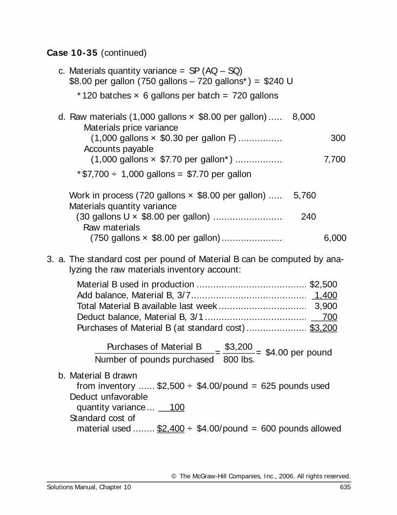
© The McGraw-Hill Companies, Inc., 2006. All rights reserved.
Solutions Manual, Chapter 10 635
Case 10-35 (continued)
c. Materials quantity variance = SP (AQ – SQ) $8.00 per gallon (750 gallons – 720 gallons*) = $240 U
*120 batches × 6 gallons per batch = 720 gallons
d. Raw materials (1,000 gallons × $8.00 per gallon) ...... 8,000
Materials price variance
(1,000 gallons × $0.30 per gallon F) ................. 300
Accounts payable
(1,000 gallons × $7.70 per gallon*) .................. 7,700
*$7,700 ÷ 1,000 gallons = $7.70 per gallon
Work in process (720 gallons × $8.00 per gallon) ...... 5,760 Materials quantity variance
(30 gallons U × $8.00 per gallon) .......................... 240 Raw materials
(750 gallons × $8.00 per gallon)....................... 6,000 3. a. The standard cost per pound of Material B can be computed by ana-
lyzing the raw materials inventory account:
Material B used in production ........................................ $2,500Add balance, Material B, 3/7.......................................... 1,400Total Material B available last week ................................ 3,900Deduct balance, Material B, 3/1 ..................................... 700Purchases of Material B (at standard cost) ...................... $3,200
Purchases of Material B $3,200
= = $4.00 per poundNumber of pounds purchased 800 lbs.
b.
Material B drawn from inventory ...... $2,500 ÷ $4.00/pound = 625 pounds used
Deduct unfavorable
quantity variance ... 100
Standard cost of
material used ........ $2,400 ÷ $4.00/pound = 600 pounds allowed
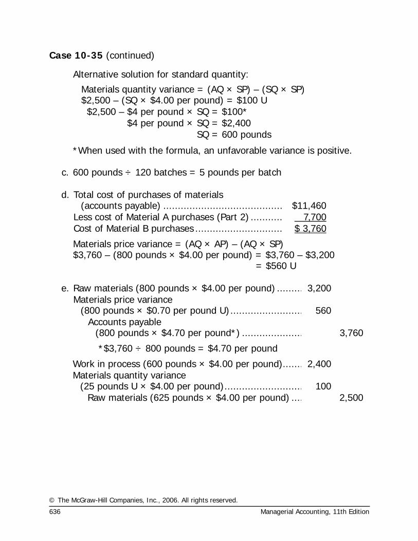
© The McGraw-Hill Companies, Inc., 2006. All rights reserved.
636 Managerial Accounting, 11th Edition
Case 10-35 (continued)
Alternative solution for standard quantity:
Materials quantity variance = (AQ × SP) – (SQ × SP) $2,500 – (SQ × $4.00 per pound) = $100 U
$2,500 – $4 per pound × SQ = $100* $4 per pound × SQ = $2,400
SQ = 600 pounds
*When used with the formula, an unfavorable variance is positive. c. 600 pounds ÷ 120 batches = 5 pounds per batch
d.
Total cost of purchases of materials (accounts payable) ......................................... $11,460
Less cost of Material A purchases (Part 2) ........... 7,700 Cost of Material B purchases .............................. $ 3,760
Materials price variance = (AQ × AP) – (AQ × SP) $3,760 – (800 pounds × $4.00 per pound) = $3,760 – $3,200 = $560 U
e. Raw materials (800 pounds × $4.00 per pound) ......... 3,200
Materials price variance
(800 pounds × $0.70 per pound U)......................... 560
Accounts payable
(800 pounds × $4.70 per pound*) ..................... 3,760
*$3,760 ÷ 800 pounds = $4.70 per pound
Work in process (600 pounds × $4.00 per pound)....... 2,400 Materials quantity variance
(25 pounds U × $4.00 per pound)........................... 100 Raw materials (625 pounds × $4.00 per pound) .... 2,500
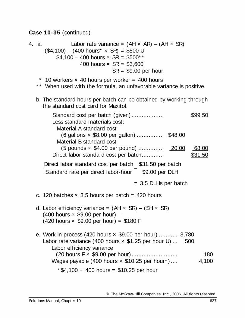
© The McGraw-Hill Companies, Inc., 2006. All rights reserved.
Solutions Manual, Chapter 10 637
Case 10-35 (continued)
4. a. Labor rate variance = (AH × AR) – (AH × SR) ($4,100) – (400 hours* × SR) = $500 U $4,100 – 400 hours × SR = $500** 400 hours × SR = $3,600 SR = $9.00 per hour
* 10 workers × 40 hours per worker = 400 hours ** When used with the formula, an unfavorable variance is positive.
b. The standard hours per batch can be obtained by working through
the standard cost card for Maxitol.
Standard cost per batch (given)................... $99.50Less standard materials cost:
Material A standard cost (6 gallons × $8.00 per gallon) ................ $48.00
Material B standard cost (5 pounds × $4.00 per pound) ............... 20.00 68.00
Direct labor standard cost per batch............. $31.50
Direct labor standard cost per batch $31.50 per batch=
Standard rate per direct labor-hour $9.00 per DLH
= 3.5 DLHs per batch
c. 120 batches × 3.5 hours per batch = 420 hours d. Labor efficiency variance = (AH × SR) – (SH × SR) (400 hours × $9.00 per hour) – (420 hours × $9.00 per hour) = $180 F
e. Work in process (420 hours × $9.00 per hour) ........... 3,780 Labor rate variance (400 hours × $1.25 per hour U) ... 500
Labor efficiency variance
(20 hours F × $9.00 per hour)........................... 180 Wages payable (400 hours × $10.25 per hour*) .... 4,100
*$4,100 ÷ 400 hours = $10.25 per hour
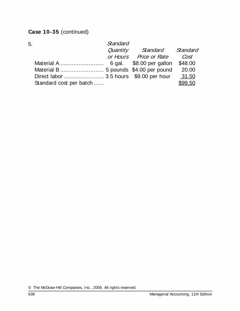
© The McGraw-Hill Companies, Inc., 2006. All rights reserved.
638 Managerial Accounting, 11th Edition
Case 10-35 (continued)
5.
Standard Quantity or Hours
Standard Price or Rate
Standard Cost
Material A ........................... 6 gal. $8.00 per gallon $48.00 Material B ...........................5 pounds $4.00 per pound 20.00 Direct labor .........................3.5 hours $9.00 per hour 31.50 Standard cost per batch ....... $99.50
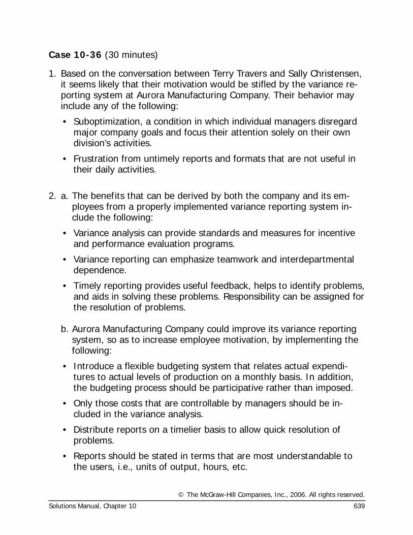
© The McGraw-Hill Companies, Inc., 2006. All rights reserved.
Solutions Manual, Chapter 10 639
Case 10-36 (30 minutes)
1. Based on the conversation between Terry Travers and Sally Christensen, it seems likely that their motivation would be stifled by the variance re-porting system at Aurora Manufacturing Company. Their behavior may include any of the following:
• Suboptimization, a condition in which individual managers disregard major company goals and focus their attention solely on their own division’s activities.
• Frustration from untimely reports and formats that are not useful in their daily activities.
2. a. The benefits that can be derived by both the company and its em-
ployees from a properly implemented variance reporting system in-clude the following:
• Variance analysis can provide standards and measures for incentive and performance evaluation programs.
• Variance reporting can emphasize teamwork and interdepartmental dependence.
• Timely reporting provides useful feedback, helps to identify problems, and aids in solving these problems. Responsibility can be assigned for the resolution of problems.
b. Aurora Manufacturing Company could improve its variance reporting
system, so as to increase employee motivation, by implementing the following:
• Introduce a flexible budgeting system that relates actual expendi-tures to actual levels of production on a monthly basis. In addition, the budgeting process should be participative rather than imposed.
• Only those costs that are controllable by managers should be in-cluded in the variance analysis.
• Distribute reports on a timelier basis to allow quick resolution of problems.
• Reports should be stated in terms that are most understandable to the users, i.e., units of output, hours, etc.
© The McGraw-Hill Companies, Inc., 2006. All rights reserved.
640 Managerial Accounting, 11th Edition
Group Exercise 10-37 The answers to the questions in this group exercise will depend on the par-ticular auto repair company that is investigated.
© The McGraw-Hill Companies, Inc., 2006. All rights reserved.
Solutions Manual, Chapter 10 641
Group Exercise 10-38 The answers to the questions in this group exercise will depend on the par-ticular company that is investigated.


![Chapter 10 SOLUTIONS - WordPress.com Chapter 10 Problem Set Chapter 10 SOLUTIONS 1. [C, None, 9.2] For the circuit in Figure 0.1, assume a unit delay through the Register and Logic](https://img.pdfslide.net/doc/110x75/5aa2cb297f8b9a46238d8563/chapter-10-solutions-chapter-10-problem-set-chapter-10-solutions-1-c-none.jpg)