Embed Size (px)
Citation preview
Chapter 12 Contents
Page
A. INTRODUCTION XII-1
B. EXTENDTM XII-1
C. APPROACH XII-2
D. THE TWO MODELS XII-3
E. AREA OF ANALYSIS XII-5
F. FACTORS THAT WERE TAKEN INTO ACCOUNT IN THE MODEL XII-6
G. LIMITATIONS OF MODELS XII-8
H. VALIDATION OF MODEL XII-9
I. SCENARIO XII-10
J. USER INPUT XII-10
K. DESIGN OF EXPERIMENT XII-11
L. CONCLUSION XII-13
M. RECOMMENDATIONS XII-14
APPENDIX
12-1 EXTENDTM EXWAR MODEL
12-2 ATTRITION RATE VIS-A-VIS PROBABILISTIC ATTRITION
12-3 VALIDATION OF MODELS DATA
12-4 USER INPUT DATA
12-5 THE EXWAR DOE MATRIX
12-6 DESIGN AND NOISE FACTORS
LIST OF FIGURES
Figure XII-1 ExWar Overview State Diagram
Figure XII-2 Planned Architecture State Diagram
Figure XII-3 Planned/Conceptual Architecture State Diagram
Figure 12-1-1 Overview of the ExWar Model
Figure 12-1-2 Overview of the Communications Layer
Figure 12-1-3 Overview of CONUS Processes
Figure 12-1-4 Overview of Forward Deployed Forces Processes
Figure12-1-5 Overview of Offshore Base Processes
Figure 12-1-6 Overview of Assembly Area Processes
Figure 12-1-7 Overview of Launching Area Processes
Figure 12-1-8 Overview of Interactions with External Nodes
Figure 12-1-9 Overview of Sea Base Processes
Figure 12-1-10 Overview of Beach Processes
Figure 12-1-11 Overview of Iron Mountain Processes
Figure 12-1-12 Overview of Objective Processes

Figure 12-2-1 Plot of Comparison Between Attrition Rate and Probabilistic Attrition
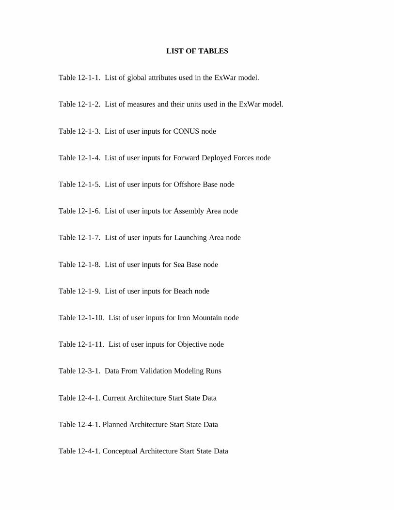
LIST OF TABLES
Table 12-1-1. List of global attributes used in the ExWar model.
Table 12-1-2. List of measures and their units used in the ExWar model.
Table 12-1-3. List of user inputs for CONUS node
Table 12-1-4. List of user inputs for Forward Deployed Forces node
Table 12-1-5. List of user inputs for Offshore Base node
Table 12-1-6. List of user inputs for Assembly Area node
Table 12-1-7. List of user inputs for Launching Area node
Table 12-1-8. List of user inputs for Sea Base node
Table 12-1-9. List of user inputs for Beach node
Table 12-1-10. List of user inputs for Iron Mountain node
Table 12-1-11. List of user inputs for Objective node
Table 12-3-1. Data From Validation Modeling Runs
Table 12-4-1. Current Architecture Start State Data
Table 12-4-1. Planned Architecture Start State Data
Table 12-4-1. Conceptual Architecture Start State Data
XII-1
XII EXPEDITIONARY WARFARE MODELING
A. INTRODUCTION
Expeditionary Warfare is one of the most complex forms of warfare, an intricate
amalgamation of air, naval, and land forces to form a powerful, mobile, far-reaching, and
quick-reacting power-projection force. An Expeditionary Force is synonymous with a
system of systems, where all the elements within it are intricately linked such that any
deficiency in one area will have an immense impact on the overall capability of the
Expeditionary Force.
To enable a systematic and comprehensive study of Expeditionary Warfare
(ExWar) and the factors that affect its performance, a simulation model was built with
EXTENDTM; a discrete event simulation tool. The model emulates the end-to-end
processes involved in accumulating, assembling, deploying, and sustaining Expeditionary
Forces ashore. It provided a means for full accounting of all the moving parts and their
interactions within the ExWar system and allowed studies into the variability inherent in
all these processes.
Useful data were obtained by running the model using an appropriate Design of
Experiment (DOE) (see A Primer on the Taguchi Method, (Ranjit Roy, (1990)), and these
data were used in a Minitab statistical program in which component systems that have the
most impact on the overall effectiveness of an Expeditionary Force were identified and
analyzed.
In addition, the EXTENDTM models were also extensively used in the excursion
studies on The Effects of Sea Basing and The Effects of Speed. Modeling runs produced
substantial data to support these studies and further reinforced their analytical effort.
B. EXTENDTM
Imagine That!’s EXTENDTM is a software program that supports developing
dynamic simulation models of complex processes. An EXTENDTM model is composed
of components, or blocks, and their interconnections, which allows simulation of large,
complex processes involving a wide variety of platforms and materials. Construction of a
XII-2
large-scale, detailed EXTENDTM model emulating the entire Expeditionary Operation,
enabled the study of emergent behavior and the investigation of non- linear effects on the
ExWar system.
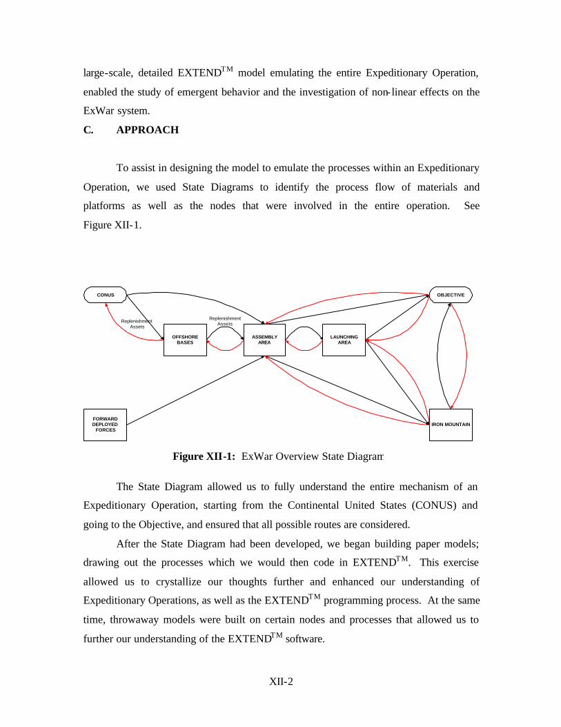
C. APPROACH
To assist in designing the model to emulate the processes within an Expeditionary
Operation, we used State Diagrams to identify the process flow of materials and
platforms as well as the nodes that were involved in the entire operation. See
Figure XII-1.
The State Diagram allowed us to fully understand the entire mechanism of an
Expeditionary Operation, starting from the Continental United States (CONUS) and
going to the Objective, and ensured that all possible routes are considered.
After the State Diagram had been developed, we began building paper models;
drawing out the processes which we would then code in EXTENDTM. This exercise
allowed us to crystallize our thoughts further and enhanced our understanding of
Expeditionary Operations, as well as the EXTENDTM programming process. At the same
time, throwaway models were built on certain nodes and processes that allowed us to
further our understanding of the EXTENDTM software.
CONUS
OFFSHOREBASES
ASSEMBLYAREA
FORWARDDEPLOYED
FORCES
LAUNCHINGAREA
IRON MOUNTAIN
OBJECTIVE
ReplenishmentAssets
ReplenishmentAssets
Figure XII-1: ExWar Overview State Diagram
XII-3
Throughout this planning and learning stage, we also began to work on the
questions that we wanted the EXTENDTM model to provide answers for. This is
especially important as it allowed us to focus on a common objective and to design the
model to provide specific answers to those questions.
After extensive planning and research, we came to the conclusion that instead of
building a single model that would allow us to run all types of Expeditionary concepts
and architectures, it would be simpler, both from the programmer and the user point of
view, for two models to be built instead. These two models will be constructed so that all
three architectures (Current, Planned, and Conceptual) of interest can be studied.
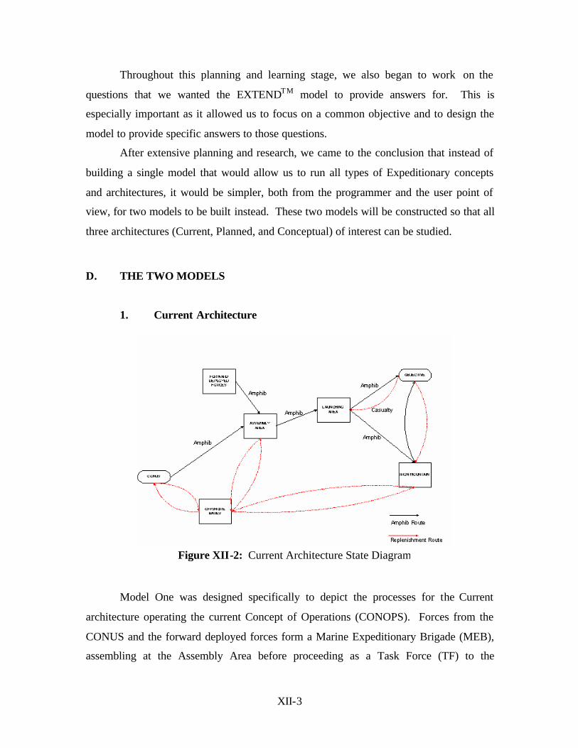
D. THE TWO MODELS
1. Current Architecture
Model One was designed specifically to depict the processes for the Current
architecture operating the current Concept of Operations (CONOPS). Forces from the
CONUS and the forward deployed forces form a Marine Expeditionary Brigade (MEB),
assembling at the Assembly Area before proceeding as a Task Force (TF) to the
Figure XII-2: Current Architecture State Diagram
XII-4
Launching Area. Once the TF arrives at the Launching Area, Marine forces will be
deployed in scheduled waves to both the Objective and the Iron Mountain. After the
Iron Mountain is secured (after a user-specified period of time), the first wave of logistic
supplies, which is provided by Maritime Pre-positioning Force (MPF) ships, supplying
logistics such as food, water, ammunition, spares, etc. will begin to arrive and commence
the building up of a logistic depot. Either LMSR ships or HSVs will carry out
subsequent logistic supplies from the Offshore Base to the Iron Mountain.
At the same time, while fighting is ongoing at the Objective, reinforcements
continue to arrive from the Iron Mountain to the Objective, supplying troops, food, water,
and ammunition. This entire operation will continue for a 90-day period.
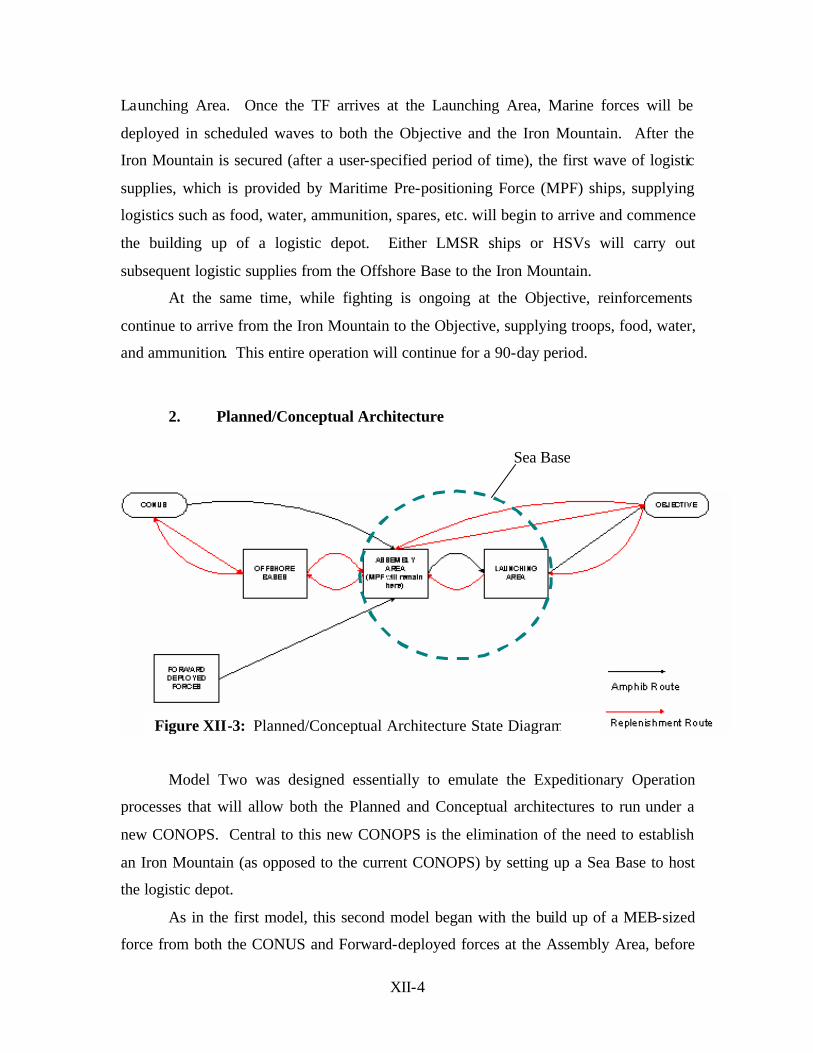
2. Planned/Conceptual Architecture
Model Two was designed essentially to emulate the Expeditionary Operation
processes that will allow both the Planned and Conceptual architectures to run under a
new CONOPS. Central to this new CONOPS is the elimination of the need to establish
an Iron Mountain (as opposed to the current CONOPS) by setting up a Sea Base to host
the logistic depot.
As in the first model, this second model began with the build up of a MEB-sized
force from both the CONUS and Forward-deployed forces at the Assembly Area, before
Sea Base
Figure XII-3: Planned/Conceptual Architecture State Diagram
XII-5
proceeding as a TF to the Launching Area. Once the TF arrives at the Launching Area,
Marine forces will be deployed in scheduled waves to the Objective. After all the
scheduled waves have been launched, the Logistic ships stationed at the Assembly Area
will begin their logistical sustainment operation. Either Light and Medium Speed
Roll-On-Roll-Off (LMSR) ships or High Speed Vessels (HSVs) will trans it between the
Offshore Base and the Assembly Area to replenish these logistic ships. This entire
operation will continue for a 90-day period. The main difference between the Planned
and Conceptual architectures is that the assets used are different. See earlier chapters for
details on the assets used in the two architectures.
E. AREA OF ANALYSIS
The driving factor in designing and building the EXTENDTM model was to
produce a useful and relevant tool for our integrated project analysis. The output data
from the models provided valuable information and insights in addressing the following
issues:
1. A Total System of Systems Analysis of the Expeditionary Warfare
Architecture
The model output provided a basis for analysis to determine the most effective
architecture among the current, planned, and future concepts, to project and sustain an
Expeditionary Force ashore.
XII-6
2. Studies of the Interfaces and Synergies Among Ships, Aircraft, and
System Within Architectures
The analysis of the combat power built up ashore and the logistical sustainment
cycle at the Sea Base/Iron Mountain provided insights about the interfaces, synergies,
and/or shortcomings among the ships, aircraft, and systems within the architectures.
3. HSV Study
Multiple runs of the model utilizing LMSRs or HSVs provided relevant data to
determine the effects of these ships on the logistical sustainment capability of the
Expeditionary Force.
4. Sea Basing
The modeling runs, based on the scenario, also provided the basis for analysis to
determine if the proposed and future concept is able to support the Sea Base concept.
5. Significant Factors in Expeditionary Architecture
Factors that have significant impact on the capability of an Expeditionary Force to
project and sustain an operation ashore can be identified through analysis of the model
output. Analysis of the model output provided useful insights on where emphasis (both
money and effort) should be placed to obtain a higher return in terms of warfighting
capability.
F. FACTORS THAT WERE TAKEN INTO ACCOUNT IN THE MODEL
To enable us to meaningfully and realistically analyze the data obtained from the
models, there is a need to ensure that most, if not all, environmental effects are accounted
for in the model. However, as it is not feasible to include each and every environmental
XII-7
factor, an essential list was drawn up to assist us during the model design stage. The
following factors are those that are taken into account in the final model coding. For
details on the model, please refer to the Appendix 12-1.
1. Environmental Effects
Effects from environmental factors such as the sea-state and weather, all play an
important role in affecting the performance of an Expeditionary force. Such effects range
from longer transit delays for ships and aircraft to longer delays in loading and unloading
cargos between ships. To account for these environmental effects, flexibility was built
into the models; which will allow the user to change the transit speed of vehicles, the
loading and unloading delays of cargos, and the reduced cargo capacity of a vehicle in a
prevailing sea-state and weather.
2. Mine Threats
Mines are a very real threat in an expeditionary operation and they affect the
speed and maneuverability of seacraft when they are transiting that area. This is
especially true when enemies will mine areas that are likely to be used as landing
beaches. To account for this effect in the models, it is assumed that a minesweeping
operation has been carried out to establish sea-lanes in which seacraft may transit safely,
but they will be limited by the number of sea- lanes available. Hence, a user may input
the number of sea-lanes available between the Launching Area, the Beach, and
Iron Mountain, respectively, depending on the threat posed by the mines.
3. Attrition/Casualty of Troops
Attrition of troops is accounted for in the various phases of the operation. The
phases include the transit from the Launching Area to the Beach or Iron Mountain, from
the Beach or Iron Mountain to the Objective, and the battle at the Iron Mountain and
Objective. Attrition is imposed not only on troops, but on vehicles as well. In the
XII-8
models, the user is able to input the attrition rate of troops as well as air, land, and sea
vehicles at the various phases, depending on the intensity of the battle. Attrition rates are
used in the models, instead of probabilistic attrition because a study conducted by us
showed that results obtained by using the former are within a 95% confidence interval of
using the latter. The advantage of using a rate instead of probability is that it eliminates
the need for multiple runs to derive a result at a statistically significant value. The details
and results of the attrition rate against probabilistic attrition can be found in
Appendix 12-2.
4. Reliability/Serviceability of Vehicles
In the real world, vehicles are routinely scheduled for preventive maintenance and
they breakdown from time to time. In the models, a user can input the reliability figure
for that particula r type of vehicle, such as aircraft, Landing Craft Air Cushion (LCAC),
etc., and he can also input the number of operating hours that a vehicle type would
operate before standing down for a certain period for preventive maintenance. This is
especially important for aircraft. This factor ensures that the number of vehicles that are
available for operation at any one time is realistic.
G. LIMITATIONS OF MODELS
EXTENDTM is a very powerful simulation program that would allow almost
unlimited variations in the modeling structure to realistically emulate an entire
expeditionary warfare operation. However, given the limited time, the two models that
were built were designed to provide specific answers to the ExWar Integrated project.
Hence, there are some limitations that were inherent to these models, which could be
further improved if given the time, when there is a need. Some of the existing limitations
in the two models are:
XII-9
1. Scheduled Assault Waves
As part of the data input prior to the simulation runs, the user is required to input
the loading plan for all the scheduled waves. These scheduled waves will form the
assault force that will be launched ashore. Hence, the result of the modeling runs will be
very much dependent on the way these scheduled assault waves are formulated. A user
would be expected to enter a realistic assault wave formation, as these models do not
have built- in checks to ensure that the loading plans for the various sea and air
transporters are correct.
2. Constant Rate of Consumption
The two models were built with a constant rate of consumption for the expendable
resources. Depending on whether it is a surge or normal consumption period, the
consumption rate of food, water, ammunition, and fuel are fixed, respectively. The
depletion of these resources is only dependent on the number of troops and the usage of
the vehicles at the various locations throughout an operation.
3. No Built-in Optimization Modules
The output from the models is a direct result of the input data going through a
chain of events within that model. There are no optimization modules built within the
models that would provide the best solution for an expeditionary operation run. For
example, in a particular run, if a user decides to run the model using a 75%/25%
allocation of air/sea assets, respectively, for the replenishment operations, the result for
that modeling run would be based on that assumption. If the user would like to know
what would the result be if the asset allocation is changed to 50%/50%, respectively, a
new run will be required. There are no built- in optimization modules in the existing
models that would give the user the optimum combination of asset allocation that will
yield the best result.
XII-10
4. General Categorization of Assets/Resources
In the two models, the resources that were emulated were placed into general
categories for easy implementation and interpretation of the output results. Examples of
this generalization include the placement of all truck types under a single truck category,
regardless of their specific capabilities or limitations; grouping ammunition into air,
ground, and naval ammunition, respectively. However, we have taken care that such
categorization would still allow the models to emulate the operation as realistically as
possible. For example, the generalization of the trucks will not eliminate the need to
transport them from the ships to shore; thereby taxing the transporter assets, and we have
also allocated only a certain percentage of these trucks for transportation purposes,
providing for the fact that some of these trucks have other roles. The models could be
further improved to depict a higher resolution of both assets and resources, but is not
currently implemented in the existing models.
H. VALIDATION OF MODEL
One of the most important steps in modeling is validation. There is a need to
validate the models to ensure that they were performing satisfactorily and producing
results that can be trusted. However, it became a challenge to find data that would allow
us to run and validate the models, as a model of this scale and complexity has never been
built to our knowledge. After an extensive search, we were able to locate modeling data
that were obtained through a model built with ARENATM (see Kelton et al., 2002), which
studied the concept of Ship to Objective Maneuver (STOM) in Sea Based logistics (see
An Analysis of STOM (Ship to Objective Maneuver) In Sea Based Logistics by Kang,
Doerr, Bryan, and Ameyugo, 2002).
We were able to run our EXTENDTM models with the data and obtained very
similar conclusions. Generally, the results from both models concluded that the logistics
sustainment for a STOM concept is highly dependent on the distance of the Sea Base
from the Objective and the amount of resources to be transported ashore. However, there
are slight differences in the exact data output as both the models from ARENATM and
XII-11
EXTENDTM have slightly different design considerations and assumptions. For example,
in the EXTENDTM model, the number of helicopter spots onboard a ship that are
available at any one time was modeled, thereby limiting the number of helicopters that
may be operating at the same time. This resulted in the EXTENDTM model being more
sensitive when the load to be transported ashore is increased. Please see Appendix 12-3
for details of the validation runs.
I. SCENARIO
To ensure that the modeling results would be as close to a real life operation as
possible, the worst case scenario out of three possible scenarios was selected to be the
setting for the modeling runs. See Chapter V for the details on the scenario used in the
modeling run.
J. USER INPUT
Based on the chosen scenario and the envisaged capabilities of the United States
Marine Corps (USMC), three sets of user input data were set up. We tried to use as much
of the official data as possible, collated through extensive research of publications and
Websites. On occasions when no formal data were available, intelligent and logical
inputs were determined. Please see Appendix 12-4 for details.
K. DESIGN OF EXPERIMENTS
An equally important part of the models is a well thought-out, systematic,
thorough, and organized approach towards the modeling runs. It would ensure that the
inputs and outputs of the model provide a useful insight into the entire ExWar system.
As ExWar is a very complex operation, with many moving components that are
constantly interacting amongst themselves, there is a need to find a methodology that
would allow a systematic approach to run the model and to obtain the desired results.
XII-12
One such methodology is the Design of Experiments (DOE) (See R.A. Fisher, 1951,
Design of Experiments).
However, as the conventional DOE method would require exhaustive modeling
runs to investigate all possible conditions and all identified factors (also known as
factorial design), it would be a very time-consuming and manpower intensive process.
To overcome this, we were able to design a DOE that is a combination of the exhaustive
factorial runs (for Design Factors) and half factorial runs (for Noise Factors) in a
standardized design array that would reduce the number of modeling runs required and
still retain the essential data within the modeling results. The decision for full factorial
runs for the Design Factors was that they were the center of gravity of our study. As
such, it would be essential that the resolution of the simulation results could allow us to
investigate the full effects and interactions between design factors. As for the
Noise Factors, we were interested in investigating the effects of noise on the performance
of the various architectures. By using half factorial, we were still able to conduct such
investigations without losing the resolution. With the optimized DOE matrix, we were
able to achieve what we had set out to do using the smallest number of simulation runs.
See Appendix 12-5 for the designed experimental matrix.
1. Experiment Factors
In the planning stage to develop the DOE for the model, several critical factors
that define the effectiveness of an Expeditionary architecture were identified; these
factors will herein be known as Design Factors. At the same time, it was also recognized
that there exist factors that were not within the control of the architect, but would still
have an effect on the effectiveness of the architecture; herein known as Noise Factors.
All of these factors are defined below, while the detailed levels in each factor can be
found in Appendix 12-6.
XII-13
a. Design Factors
Architectures - Three architectures were identified in this Expeditionary Warfare
study. In the current architecture, an Iron Mountain forms an integral part of the
CONOPS, while the STOM concept is central to the planned and future architecture, with
the main difference being the characteristics of the assets involved.
Replenishment Means - Defined as the means of replenishment to sustain the
logistics depot (Iron Mountain or Sea Base) from the Offshore Base. As the project
requires the study of the effects of using High-Speed Vehicles (HSVs) in lieu of existing
LMSR ships for such replenishment runs, these will form the design factors here. Hence,
the normalizing element will be the daily sustainment rate; i.e., one LMSR (or
replenishment ship) every five days is needed to sustain the Iron Mountain/Sea Base and
if HSV is used, two HSVs per day are required.
Ship to Objective Proximity - This is defined as the distance between the assault
forces and the objective.
b. Noise Factors
Attrition - This attrition factor will be applicable at the following locations:
Launching Area, Iron Mountain (current architecture), and the Objective. The attrition
factor will affect all vehicles and troops as designed in the EXTENDTM model.
Weather - Although in realty, the weather would have an effect in virtually
everything: in this DOE, in order to have better control over this factor and its effect on
the model output, the weather effect will be limited to the area of operation, i.e.,
Launching Area, Iron Mountain, and Objective. Hence, only the following parameters
will be affected by the weather in this DOE; transit speed of air and surface craft, loading
and unloading delays for air and surface craft, and the loading capacity of surface craft.
Mine Threat - The mine threat in the area of operations will affect the sea room
available to the Expeditionary force to project its force by seacraft. In this DOE, this
factor will affect the number of sea-lanes available between the Launching Area and the
Iron Mountain, and between Launching Area and Beachhead.
XII-14
Consumption (Ammo and Fuel) - The consumption of ammunition and fuel by a
fighting force at the Iron Mountain and Objective is directly proportional to the intensity
of the conflict (i.e., stronger resistance by an enemy force will result in a higher
consumption of ammunition and fuel by the Expeditionary force in combat).
L. CONCLUSION
The use of EXTENDTM models allows the study and comparison of systems of
systems. Although the models designed were not a complete representation of an entire
Expeditionary operation, assumptions and categorizations made in the modeling effort
still allow for a common basis of comparison between the different architectures.
Combined with an appropriate DOE, the models also allowed investigation into the
unique characteristics of each architecture, which would have been most difficult without
the model and the DOE.
However, if given more time, the models have the potential to be further
improved to a higher resolution in order to depict as close to a real operation as possible,
and thus be used as an effective planning tool for ExWar. It would allow a commander to
have a better appreciation of his force build-up time and the logistics requirements based
on his operational plan.
M. RECOMMENDATIONS
1. Variable Rate of Consumption
The consumption rate of the resources, such as food, water, ammunition, and fuel,
should be modified to be variable. This variability would inject some form of uncertainty
into the model to check that the architecture would continue to perform satisfactorily
under adverse conditions.
XII-15
2. Detailed Sea Base Modeling
Another aspect that should be fully explored using EXTENDTM is the Sea Base
concept. Detailed modeling of the entire Sea Base operation, taking into account the
layout and design of the ships, the storage capacity and design, the movement and
tracking of stores, the movement of stores across platforms, and the detail replenishment
concept of these ships, would all provide invaluable information when designing a
Sea Base.
3. EXTENDTM Model as a Planning Tool
The models may also be further improved upon to reflect all the details in an
Expeditionary operation. These could include a more accurate representation of all the
resources that are required to be transported, a more robust weather module (rather than a
fixed speed reduction rate) that affects different platforms differently and a more refined
attrition module. The models could then be used as a more robust planning guide in
future.
XII-16
REFERENCES
Imagine That!, Inc. “EXTENDTM Professional Simulation Tools, User’s Guide v5.” 2000. Fisher, R.A.. “Design of Experiment.” 1951. Roy, R. “A Primer On The Taguchi Method.” 1990. Allen, P. “Situational Force Scoring: Accounting for Combined Arms Effects in
Aggregate Combat Models.” RAND. 1992.
XII-17
LIST OF ACRONYMS AND ABBREVIATIONS
AAV Amphibious Assault Vehicle
AAAV Advanced Amphibious Assault Vehicle
Ammo Ammunition
Amphib Amphibious Units
CONOPS Concept of Operations
CONUS Continental United States
DOE Design of Experiments
ExWar Expeditionary Warfare
HSV High Speed Vessel
LAV Light Armored Vehicle
LCAC Landing Craft Air Cushion
LHA(R) Amphibious Assault Ship General Purpose (Replacement)
LHD Amphibious Assault Ship Multi-Purpose
LMSR Light and Medium Speed Roll-On-Roll-Off
MEB Marine Expeditionary Brigade
MPF Maritime Pre-positioning Force
NPS Naval Postgraduate School
STOM Ship to Objective Maneuver
TF Task Force
USMC United States Marine Corps
APPENDIX 12-1
EXTENDTM ExWar Model
12-1-1
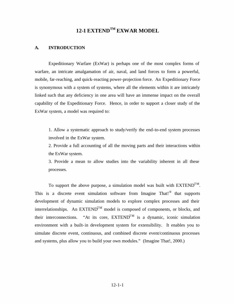
12-1 EXTENDTM EXWAR MODEL
A. INTRODUCTION
Expeditionary Warfare (ExWar) is perhaps one of the most complex forms of
warfare, an intricate amalgamation of air, naval, and land forces to form a powerful,
mobile, far-reaching, and quick-reacting power-projection force. An Expeditionary Force
is synonymous with a system of systems, where all the elements within it are intricately
linked such that any deficiency in one area will have an immense impact on the overall
capability of the Expeditionary Force. Hence, in order to support a closer study of the
ExWar system, a model was required to:
1. Allow a systematic approach to study/verify the end-to-end system processes
involved in the ExWar system.
2. Provide a full accounting of all the moving parts and their interactions within
the ExWar system.
3. Provide a mean to allow studies into the variability inherent in all these
processes.
To support the above purpose, a simulation model was built with EXTENDTM.
This is a discrete event simulation software from Imagine That!® that supports
development of dynamic simulation models to explore complex processes and their
interrelationships. An EXTENDTM model is composed of components, or blocks, and
their interconnections. “At its core, EXTENDTM is a dynamic, iconic simulation
environment with a built- in development system for extensibility. It enables you to
simulate discrete event, continuous, and combined discrete event/continuous processes
and systems, plus allow you to build your own modules.” (Imagine That!, 2000.)
12-1-2
B. OVERVIEW OF EXWAR MODEL
Forward DeployedForces
Offshore Base
Assembly Area
Launching Area
Iron Mountain Objective
CONUS
Sea Base
Note: The nodes at "Sea Base" and "Iron Mountain"are present depending on the operating concept andscenario. In the SEI-3 study, these two nodes weremutually exclusive.
Beach
Figure 12-1-1: Overview of the ExWar model
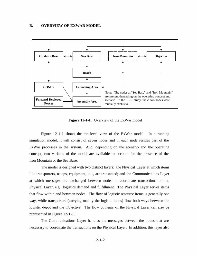
Figure 12-1-1 shows the top- level view of the ExWar model. In a running
simulation model, it will consist of seven nodes and in each node resides part of the
ExWar processes in the system. And, depending on the scenario and the operating
concept, two variants of the model are available to account for the presence of the
Iron Mountain or the Sea Base.
The model is designed with two distinct layers: the Physical Layer at which items
like transporters, troops, equipment, etc., are transacted; and the Communications Layer
at which messages are exchanged between nodes to coordinate transactions on the
Physical Layer, e.g., logistics demand and fulfillment. The Phys ical Layer serves items
that flow within and between nodes. The flow of logistic resource items is generally one
way, while transporters (carrying mainly the logistic items) flow both ways between the
logistic depot and the Objective. The flow of items on the Physical Layer can also be
represented in Figure 12-1-1.
The Communications Layer handles the messages between the nodes that are
necessary to coordinate the transactions on the Physical Layer. In addition, this layer also
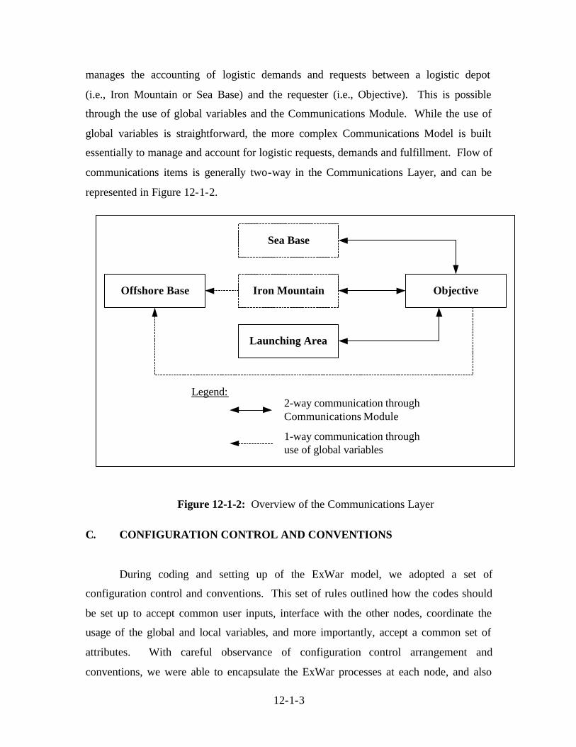
12-1-3
manages the accounting of logistic demands and requests between a logistic depot
(i.e., Iron Mountain or Sea Base) and the requester (i.e., Objective). This is possible
through the use of global variables and the Communications Module. While the use of
global variables is straightforward, the more complex Communications Model is built
essentially to manage and account for logistic requests, demands and fulfillment. Flow of
communications items is generally two-way in the Communications Layer, and can be
represented in Figure 12-1-2.
Launching Area
Iron Mountain Objective
Sea Base
Offshore Base
Legend:2-way communication throughCommunications Module
1-way communication throughuse of global variables
Figure 12-1-2: Overview of the Communications Layer
C. CONFIGURATION CONTROL AND CONVENTIONS
During coding and setting up of the ExWar model, we adopted a set of
configuration control and conventions. This set of rules outlined how the codes should
be set up to accept common user inputs, interface with the other nodes, coordinate the
usage of the global and local variables, and more importantly, accept a common set of
attributes. With careful observance of configuration control arrangement and
conventions, we were able to encapsulate the ExWar processes at each node, and also
12-1-4
facilitate independent coding by different members of the modeling group and allow
model integration.
1. Attributes
“Attributes are a very important part of a discrete event simulation. Attributes are
characteristics of an item that stay with the item as it moves through the simulation.”
(Imagine That!, 2000). In the ExWar model, there were essentially four categories of
items flowing in the simulation: Force, Transporter, Resource, and Message. We
identified each item to its type by assigning it with a unique “Object ID” (“Object ID” is
an attribute which holds a value to identify the item). We used attributes to characterize
and describe each of these items. For example, for an item in the Transporter category,
attributes like “Food,” “Ground_Ammo,” etc., described how much of the logistic
resource that the transporter was carrying.
In order to ensure inter-usage of common attributes between nodes, we created a
global list of attributes, which would hold values as results of processes carried out
within the nodes. As the item flows into another node, these attribute values would, in
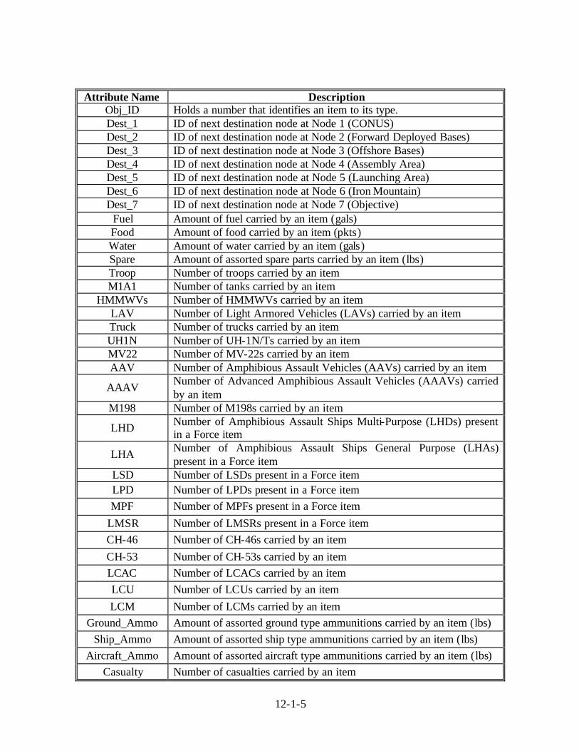
turn, become inputs for the processes for that node. A lis t of the global attributes used is
shown in Table 12-1-1.
12-1-5
Attribute Name Description Obj_ID Holds a number that identifies an item to its type. Dest_1 ID of next destination node at Node 1 (CONUS) Dest_2 ID of next destination node at Node 2 (Forward Deployed Bases) Dest_3 ID of next destination node at Node 3 (Offshore Bases) Dest_4 ID of next destination node at Node 4 (Assembly Area) Dest_5 ID of next destination node at Node 5 (Launching Area) Dest_6 ID of next destination node at Node 6 (Iron Mountain) Dest_7 ID of next destination node at Node 7 (Objective)
Fuel Amount of fuel carried by an item (gals) Food Amount of food carried by an item (pkts) Water Amount of water carried by an item (gals) Spare Amount of assorted spare parts carried by an item (lbs) Troop Number of troops carried by an item M1A1 Number of tanks carried by an item
HMMWVs Number of HMMWVs carried by an item LAV Number of Light Armored Vehicles (LAVs) carried by an item Truck Number of trucks carried by an item UH1N Number of UH-1N/Ts carried by an item MV22 Number of MV-22s carried by an item AAV Number of Amphibious Assault Vehicles (AAVs) carried by an item
AAAV Number of Advanced Amphibious Assault Vehicles (AAAVs) carried by an item
M198 Number of M198s carried by an item
LHD Number of Amphibious Assault Ships Multi-Purpose (LHDs) present in a Force item
LHA Number of Amphibious Assault Ships General Purpose (LHAs) present in a Force item
LSD Number of LSDs present in a Force item LPD Number of LPDs present in a Force item MPF Number of MPFs present in a Force item
LMSR Number of LMSRs present in a Force item CH-46 Number of CH-46s carried by an item CH-53 Number of CH-53s carried by an item LCAC Number of LCACs carried by an item LCU Number of LCUs carried by an item LCM Number of LCMs carried by an item
Ground_Ammo Amount of assorted ground type ammunitions carried by an item (lbs) Ship_Ammo Amount of assorted ship type ammunitions carried by an item (lbs)
Aircraft_Ammo Amount of assorted aircraft type ammunitions carried by an item (lbs) Casualty Number of casualties carried by an item
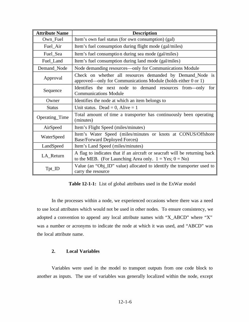
12-1-6
Attribute Name Description Own_Fuel Item’s own fuel status (for own consumption) (gal) Fuel_Air Item’s fuel consumption during flight mode (gal/miles)
Fuel_Sea Item’s fuel consumption during sea mode (gal/miles) Fuel_Land Item’s fuel consumption during land mode (gal/miles)
Demand_Node Node demanding resources—only for Communications Module
Approval Check on whether all resources demanded by Demand_Node is approved—only for Communications Module (holds either 0 or 1)
Sequence Identifies the next node to demand resources from—only for Communications Module
Owner Identifies the node at which an item belongs to Status Unit status. Dead = 0, Alive = 1
Operating_Time Total amount of time a transporter has continuously been operating (minutes)
AirSpeed Item’s Flight Speed (miles/minutes)
WaterSpeed Item’s Water Speed (miles/minutes or knots at CONUS/Offshore Base/Forward Deployed Forces)
LandSpeed Item’s Land Speed (miles/minutes)
LA_Return A flag to indicates that if an aircraft or seacraft will be returning back to the MEB. (For Launching Area only. 1 = Yes; 0 = No)
Tpt_ID Value (an “Obj_ID” value) allocated to identify the transporter used to carry the resource
Table 12-1-1: List of global attributes used in the ExWar model
In the processes within a node, we experienced occasions where there was a need
to use local attributes which would not be used in other nodes. To ensure consistency, we
adopted a convention to append any local attribute names with “X_ABCD” where “X”
was a number or acronyms to indicate the node at which it was used, and “ABCD” was
the local attribute name.
2. Local Variables
Variables were used in the model to transport outputs from one code block to
another as inputs. The use of variables was generally localized within the node, except
12-1-7
for use in the communications layer. In order to coordinate the usage of variable names
in the model, similar convention as for the local attribute names were adopted.
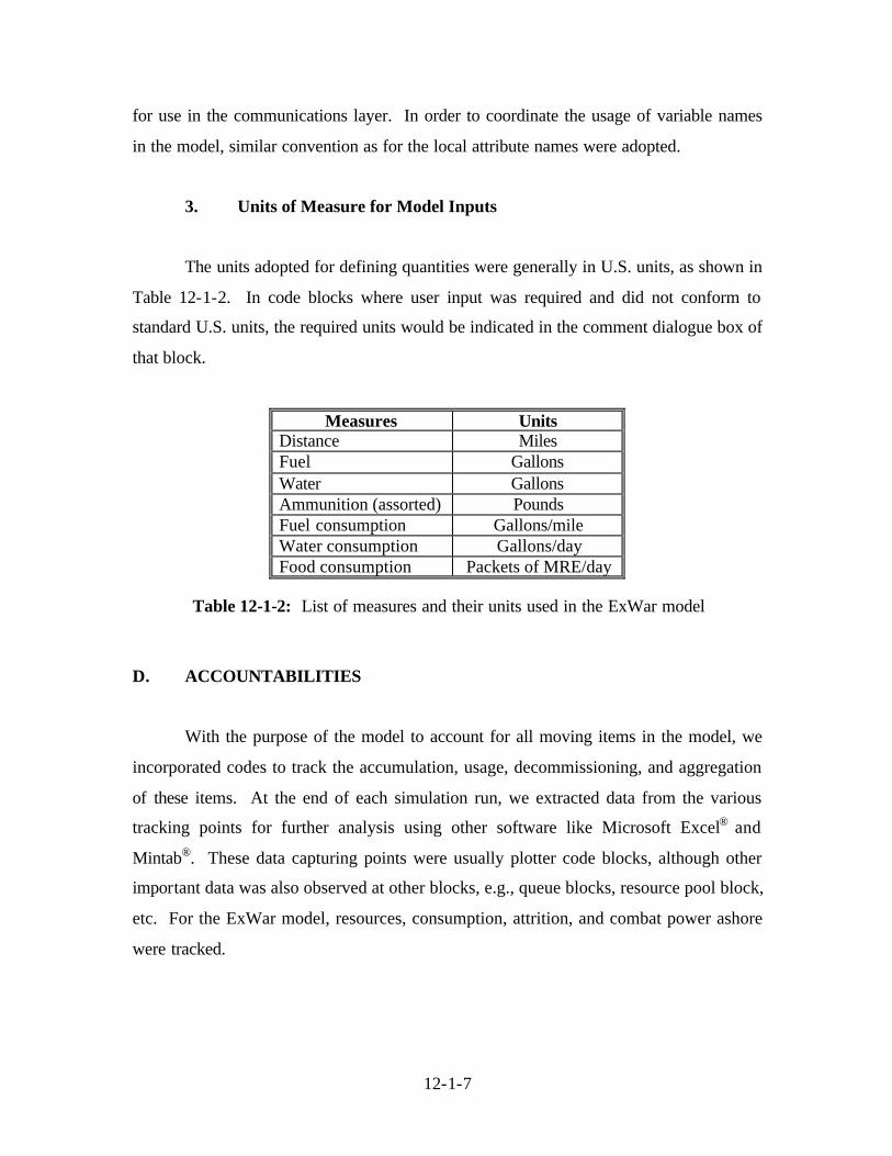
3. Units of Measure for Model Inputs
The units adopted for defining quantities were generally in U.S. units, as shown in
Table 12-1-2. In code blocks where user input was required and did not conform to
standard U.S. units, the required units would be indicated in the comment dialogue box of
that block.
Measures Units Distance Miles Fuel Gallons Water Gallons Ammunition (assorted) Pounds Fuel consumption Gallons/mile Water consumption Gallons/day Food consumption Packets of MRE/day
Table 12-1-2: List of measures and their units used in the ExWar model
D. ACCOUNTABILITIES
With the purpose of the model to account for all moving items in the model, we
incorporated codes to track the accumulation, usage, decommissioning, and aggregation
of these items. At the end of each simulation run, we extracted data from the various
tracking points for further analysis using other software like Microsoft Excel® and
Mintab®. These data capturing points were usually plotter code blocks, although other
important data was also observed at other blocks, e.g., queue blocks, resource pool block,
etc. For the ExWar model, resources, consumption, attrition, and combat power ashore
were tracked.
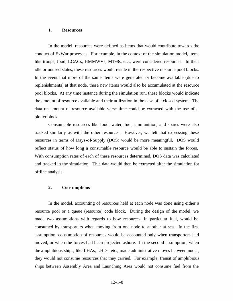
12-1-8
1. Resources
In the model, resources were defined as items that would contribute towards the
conduct of ExWar processes. For example, in the context of the simulation model, items
like troops, food, LCACs, HMMWVs, M198s, etc., were considered resources. In their
idle or unused states, these resources would reside in the respective resource pool blocks.
In the event that more of the same items were generated or become available (due to
replenishments) at that node, these new items would also be accumulated at the resource
pool blocks. At any time instance during the simulation run, these blocks would indicate
the amount of resource available and their utilization in the case of a closed system. The
data on amount of resource available verse time could be extracted with the use of a
plotter block.
Consumable resources like food, water, fuel, ammunition, and spares were also
tracked similarly as with the other resources. However, we felt that expressing these
resources in terms of Days-of-Supply (DOS) would be more meaningful. DOS would
reflect status of how long a consumable resource would be able to sustain the forces.
With consumption rates of each of these resources determined, DOS data was calculated
and tracked in the simulation. This data would then be extracted after the simulation for
offline analysis.
2. Cons umptions
In the model, accounting of resources held at each node was done using either a
resource pool or a queue (resource) code block. During the design of the model, we
made two assumptions with regards to how resources, in particular fuel, would be
consumed by transporters when moving from one node to another at sea. In the first
assumption, consumption of resources would be accounted only when transporters had
moved, or when the forces had been projected ashore. In the second assumption, when
the amphibious ships, like LHAs, LHDs, etc., made administrative moves between nodes,
they would not consume resources that they carried. For example, transit of amphibious
ships between Assembly Area and Launching Area would not consume fuel from the
12-1-9
stockpile that they would be carrying. We made this reasonable assumption because
replenishments of these ships are made through the existing CLF assets (which were not
modeled). The second assumption was held valid for ships making administrative transit
between the CONUS, Offshore Base, Assembly Area, Launching Area, and Sea Base
nodes.
Between Launching Area, Sea Base, Iron Mountain, and Objective nodes,
transporters (e.g., LCACs, AAVs, etc.) would consume the fuel resource, and the
transporter’s originating node (defined by the item attribute “Owner”) would be
responsible for replenishing the transporter’s fuel when it returned from its mission. In
addition, in order to account for the maintenance necessary to keep the transporters
operating, the spares resource would also be consumed at the Launching Area, Sea Base,
and Iron Mountain nodes.
For the forces projected ashore, the troops would consume both water and food,
measured in gallons and number of packets of Meals-Ready-to-Eat (MRE), respectively.
In the model, we accounted for these consumptions once every 24 hours, and the
respective resource pools would be deducted by the daily consumption rate. Similarly,
the consumption of fuel, ground ammunition, air ammunition, and spares were also
accounted for every 24 hours, both at the Iron Mountain and the Objective.
Due to the complexity in accounting for the consumption of the primary resources
(fuel, ground ammunition, aircraft ammunition, and spares), an averaging technique was
used to determine the rate of consumption for these resources. Based on data collected
from previous conflicts (NATOPS Flight Manual Navy Model 1989, 1998, 2000, 2001;
MAGTF Planner’s Reference 2001; Jane’s Online), the total amount of resources
consumed was calculated and an average consumption rate was determined based on the
duration of the conflicts. To account for initial surge in the resource consumption rate in
order to reflect the necessary suppression fires and combat maneuvers for projection of
forces ashore, we increased the average consumption rates by 50%.
12-1-10
3. Attrition
One of the most distinct features of the ExWar model is the accounting of attrition
of transporter assets and the impact of this attrition on the sustainment of forces ashore.
Most combat simulation models only account for the attrition of combat forces and fail to
include the logistics assets, which play an important role in sustaining the force.
In the ExWar model, the attrition of the combat forces occurred at the objective as
well as the Iron Mountain, and the attrition rates was varied based on the expected
intensity of the battle, and the time lapsed since the commencement of the expeditionary
operation. The detailed description of the implementation of the attrition of the combat
forces can be found in the attrition module of the Objective Node.
The attrition of the transporter assets and vehicles occurred as they transited
between the various nodes. In the construct of the model, our assumption was that there
would only be attrition of these vehicles between the Launching Area, Iron Mountain,
and the Objective Nodes due to engagements with the enemies. Another assumption
made was that the node where the vehicle originated would not be notified of the
attrition, and thus the node would not generate another sortie or convoy to replace the
unit(s) destroyed due to attrition during transit. To account for all transporter assets at
each node, a common transit attrition module was implemented for the Launching Area,
Iron Mountain, and Objective Nodes. In the transit attrition module, the attrition rate
would determine whether a particular transporter asset or vehicle would be destroyed due
to enemy action. If the vehicle did not fall victim to enemy engagements, it would be
allowed to continue to its intended destination; however, if it were destroyed, the
transporter or vehicle would then be sent back to its originating node for accounting and
removal from the simulation pool. Details of this implementation can be found in the
Launching Area, Iron Mountain, and Objective Nodes.
4. Combat Power Ashore (CPA)
CPA was one of the outputs from the ExWar model. CPA is the aggregated score
to reflect the level of firepower available at a location. In order to calculate CPA, the
12-1-11
combat units contributing towards overall firepower were identified, and their respective
Combat Power Indexes (CPI) were also determined (see Appendix 13-1 for calculation of
CPIs). The CPI is the relative score assigned to individual combat unit, which weighs its
contribution towards CPA. With the CPIs of each type of combat unit determined, CPA
would be calculated based on the aggregated values of all the CPIs.
In the ExWar model, we measured the CPA at the Objective. This was because
the rate of CPA built-up at the Objective was of interest to our study in order to
determine the performance of the design factors, as well as the effects of noise factors.
E. FUNCTIONALITY DESCRIPTIONS OF PRINCIPLE NODES IN EXWAR
MODEL
1. CONUS
a. Process Overview
This is one of the start points of the whole ExWar model. It is at this node that
the amphibious force, consisting of LHAs, LHDs, LPDs, and/or LSDs, begins its journey
to the assembly area where preparations for amphibious assault will be conducted.
Depending on the type of ExWar architecture being investigated, this node also provides
the initial waves of MPF ships will also be projected from CONUS to the
Assembly Area. The other function of this node is also to provide replenishment runs to
the Offshore Base, which provides forward logistic support to the amphibious force at the
Assembly Area or the Iron Mountain. The process overview at CONUS is shown in
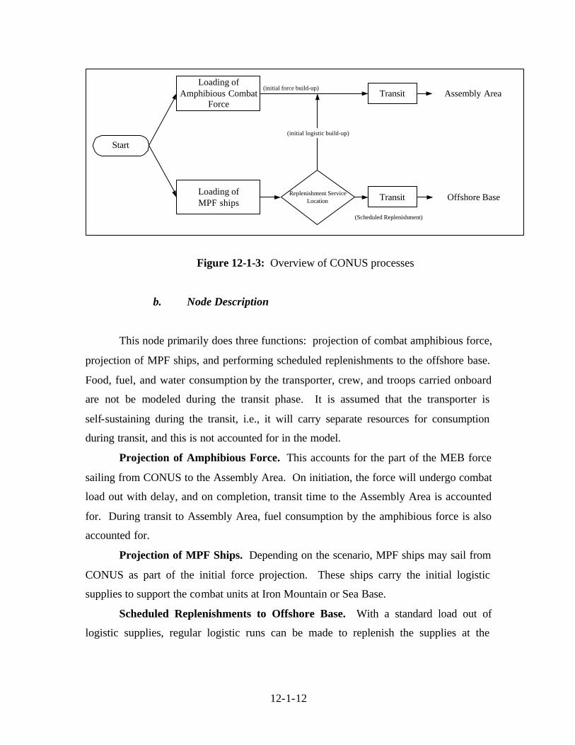
Figure 12-1-3.
12-1-12
Start
Loading ofAmphibious Combat
Force
Loading ofMPF ships
Replenishment ServiceLocation
(initial logistic build-up)
(Scheduled Replenishment)
(initial force build-up)Transit
Transit
Assembly Area
Offshore Base
Figure 12-1-3: Overview of CONUS processes
b. Node Description
This node primarily does three functions: projection of combat amphibious force,
projection of MPF ships, and performing scheduled replenishments to the offshore base.
Food, fuel, and water consumption by the transporter, crew, and troops carried onboard
are not be modeled during the transit phase. It is assumed that the transporter is
self-sustaining during the transit, i.e., it will carry separate resources for consumption
during transit, and this is not accounted for in the model.
Projection of Amphibious Force. This accounts for the part of the MEB force
sailing from CONUS to the Assembly Area. On initiation, the force will undergo combat
load out with delay, and on completion, transit time to the Assembly Area is accounted
for. During transit to Assembly Area, fuel consumption by the amphibious force is also
accounted for.
Projection of MPF Ships. Depending on the scenario, MPF ships may sail from
CONUS as part of the initial force projection. These ships carry the initial logistic
supplies to support the combat units at Iron Mountain or Sea Base.
Scheduled Replenishments to Offshore Base. With a standard load out of
logistic supplies, regular logistic runs can be made to replenish the supplies at the
12-1-13
Offshore Base. The scheduled runs will be initiated when amphibious forces have landed
at the Iron Mountain or at the Objective.
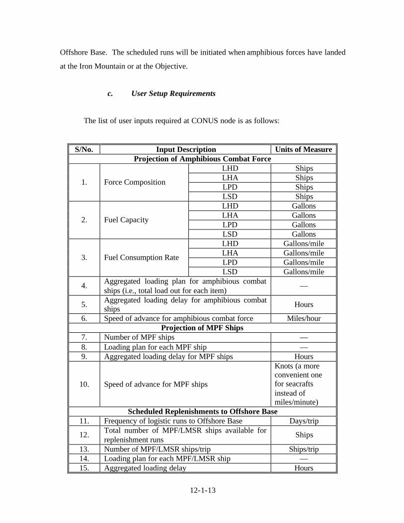
c. User Setup Requirements
The list of user inputs required at CONUS node is as follows:
S/No. Input Description Units of Measure Projection of Amphibious Combat Force
LHD Ships LHA Ships LPD Ships
1. Force Composition
LSD Ships LHD Gallons LHA Gallons LPD Gallons
2. Fuel Capacity
LSD Gallons LHD Gallons/mile LHA Gallons/mile LPD Gallons/mile
3. Fuel Consumption Rate
LSD Gallons/mile
4. Aggregated loading plan for amphibious combat ships (i.e., total load out for each item)
—
5. Aggregated loading delay for amphibious combat ships Hours
6. Speed of advance for amphibious combat force Miles/hour Projection of MPF Ships
7. Number of MPF ships — 8. Loading plan for each MPF ship — 9. Aggregated loading delay for MPF ships Hours
10. Speed of advance for MPF ships
Knots (a more convenient one for seacrafts instead of miles/minute)
Scheduled Replenishments to Offshore Base 11. Frequency of logistic runs to Offshore Base Days/trip
12. Total number of MPF/LMSR ships available for replenishment runs
Ships
13. Number of MPF/LMSR ships/trip Ships/trip 14. Loading plan for each MPF/LMSR ship — 15. Aggregated loading delay Hours

12-1-14
S/No. Input Description Units of Measure
16. Speed of advance for MPF/LMSR ships
Knots (a more convenient one for seacrafts instead of miles/minute)
17. Total number of MPF/LMSR ships available for conducting replenishment runs Ships
Table 12-1-3: List of user inputs for CONUS node
d.
At the Node Input
Since this node is a starting point for the ExWar model, there will essentially be
no input expected from other nodes. However, this node does send ships to the Offshore
Base node to replenish it’s the Offshore Base node's resources at regular intervals.
Hence, there is an input channel to receive returning replenishment assets originating
from CONUS node.
e. At the Node Output
The output from this node will be a combat unit transiting to the Assembly Area.
In addition, replenishment ships will also be generated at a pre-defined interval to depart
for the Offshore Base.
12-1-15
2. Forward Deployed Forces
a. Process Overview
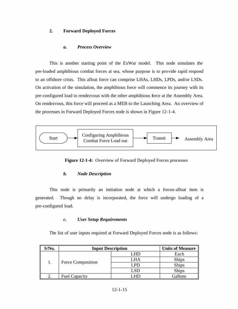
This is another starting point of the ExWar model. This node simulates the
pre-loaded amphibious combat forces at sea, whose purpose is to provide rapid respond
to an offshore crisis. This afloat force can comprise LHAs, LHDs, LPDs, and/or LSDs.
On activation of the simulation, the amphibious force will commence its journey with its
pre-configured load to rendezvous with the other amphibious force at the Assembly Area.
On rendezvous, this force will proceed as a MEB to the Launching Area. An overview of
the processes in Forward Deployed Forces node is shown in Figure 12-1-4.
StartConfiguring AmphibiousCombat Force Load out Transit Assembly Area
Figure 12-1-4: Overview of Forward Deployed Forces processes
b. Node Description
This node is primarily an initiation node at which a forces-afloat item is
generated. Though no delay is incorporated, the force will undergo loading of a
pre-configured load.
c. User Setup Requirements
The list of user inputs required at Forward Deployed Forces node is as follows:
S/No. Input Description Units of Measure LHD Each LHA Ships LPD Ships
1. Force Composition
LSD Ships 2. Fuel Capacity LHD Gallons
12-1-16
S/No. Input Description Units of Measure LHA Gallons LPD Gallons
LSD Gallons LHD Gallons/mile LHA Gallons/mile LPD Gallons/mile
3. Fuel Consumption Rate
LSD Gallons/mile
4. Aggregated loading plan for amphibious combat ships (i.e., total load out for each item) —
5. Speed of advance for amphibious combat force
Knots (a more convenient one for seacrafts instead of miles/minute)
Table 12-1-4: List of user inputs for Forward Deployed Forces node
d. At the Node Input
This is a start point of the simulation. Hence, there will not be inputs received
from other nodes during the simulation.
e. At the Node Output
The output from this node will be a pre-configured combat unit transiting to the
assembly area.
3. Offshore Base
a. Process Overview
This is a forward logistic base set up to support the forces at Iron Mountain, or at
Assembly Area/Launching Area depending on the prevailing CONOPS. This forward
logistic base is, in turn, supported by regular replenishments from CONUS. This node
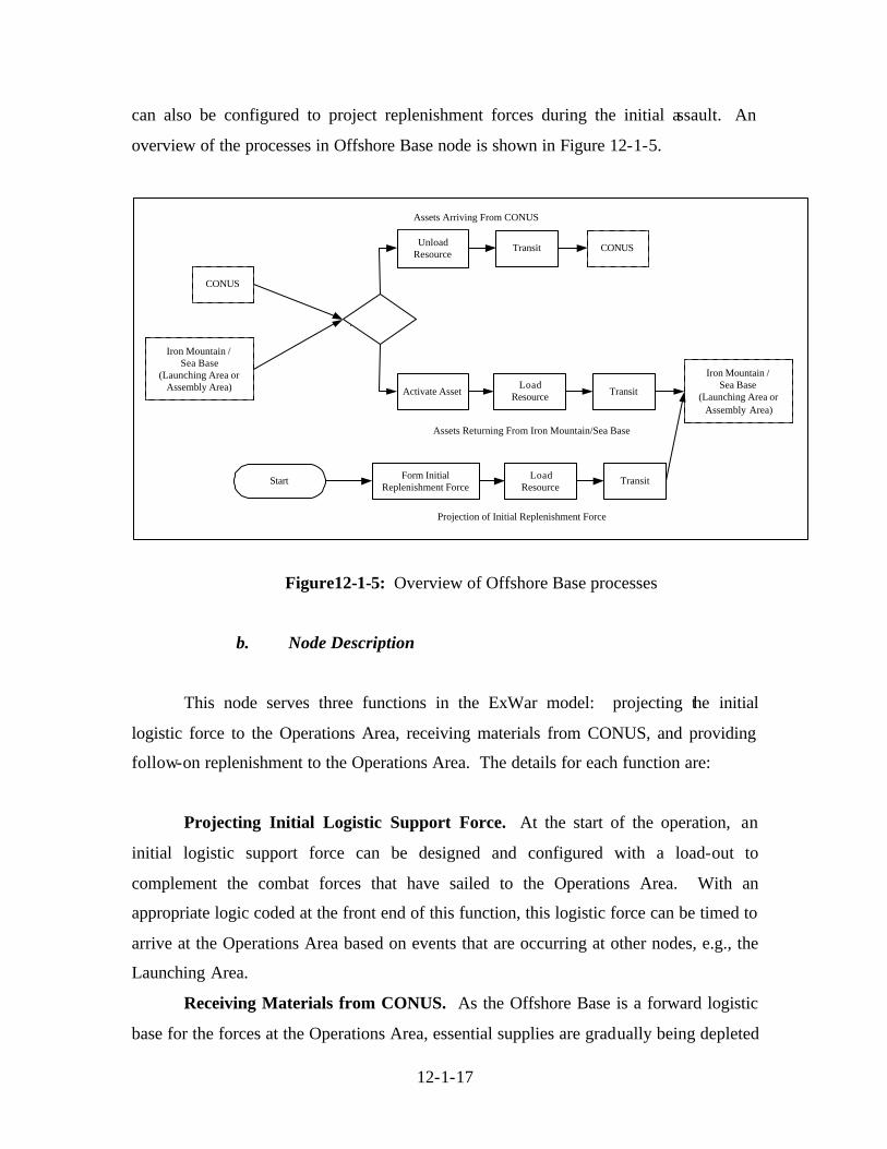
12-1-17
can also be configured to project replenishment forces during the initial assault. An
overview of the processes in Offshore Base node is shown in Figure 12-1-5.
CONUS
Iron Mountain /Sea Base
(Launching Area orAssembly Area)
UnloadResource
LoadResource
Transit
Assets Arriving From CONUS
Assets Returning From Iron Mountain/Sea Base
Transit
CONUS
Iron Mountain /Sea Base
(Launching Area orAssembly Area)
Activate Asset
LoadResource
TransitForm InitialReplenishment Force
Start
Projection of Initial Replenishment Force
Figure12-1-5: Overview of Offshore Base processes
b. Node Description
This node serves three functions in the ExWar model: projecting the initial
logistic force to the Operations Area, receiving materials from CONUS, and providing
follow-on replenishment to the Operations Area. The details for each function are:
Projecting Initial Logistic Support Force. At the start of the operation, an
initial logistic support force can be designed and configured with a load-out to
complement the combat forces that have sailed to the Operations Area. With an
appropriate logic coded at the front end of this function, this logistic force can be timed to
arrive at the Operations Area based on events that are occurring at other nodes, e.g., the
Launching Area.
Receiving Materials from CONUS. As the Offshore Base is a forward logistic
base for the forces at the Operations Area, essential supplies are gradually being depleted
12-1-18
as supplies are regularly being sent to support these forward forces. Hence, to sustain
healthy levels of supplies at the Offshore Base, logistic ships from CONUS will arrive
regularly to support the Offshore Base. When these ships arrive at the Offshore Base,
unloading delay will be incorporated when supplies are offloaded into the local
warehouses (which are represented by the “resource pool” block in EXTENDTM). On
completion of unloading, the supply ships will be sent back to the originator at CONUS.
Providing Follow-on Replenishment to the Operation Area. Besides having
the ability to launch the initial logistic force to the Iron Mountain or Sea Base, the
Offshore Base can also be configured to provide follow-on logistic support to the
Iron Mountain or Sea Base. This follow-on support is provided through regular
replenishment runs with a standard load-out using a choice of transporter, e.g., LMSR or
HSV. These follow-on logistic runs will be initiated at a preset interval after the initial
logistic force has been launched. After off- loading at the destination, these transporters
will be sent back for re-use.
c. User Setup Requirements
The list of user inputs required at Offshore Base node is as follows:
S/No. Input Description Units of Measure Projecting Initial Logistic Support Force
1. Time of initiation of logistic force xth Day
2. Aggregated loading plan (i.e., total load-out for each item) —
3. Aggregated loading delay Hours
4. Speed of advance
Knots (a more convenient one for seacrafts instead of miles/minute)
5. Destination node (to be the same as follow-on replenishment) —
Receiving Materials from CONUS 6. Aggregated unloading delay Days
12-1-19
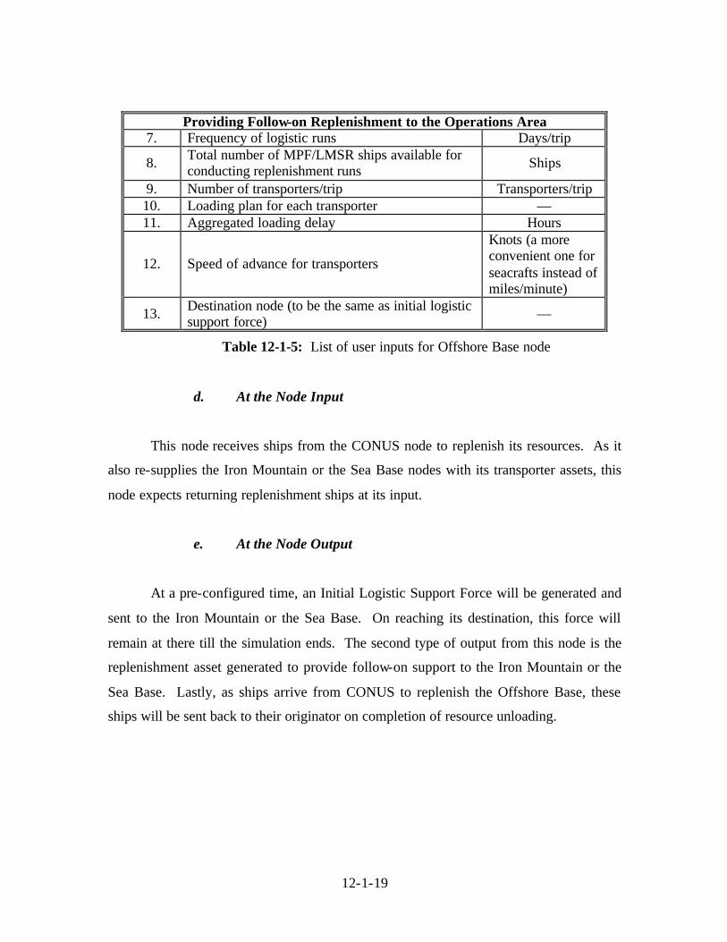
Providing Follow-on Replenishment to the Operations Area 7. Frequency of logistic runs Days/trip
8. Total number of MPF/LMSR ships available for conducting replenishment runs Ships
9. Number of transporters/trip Transporters/trip 10. Loading plan for each transporter — 11. Aggregated loading delay Hours
12. Speed of advance for transporters
Knots (a more convenient one for seacrafts instead of miles/minute)
13. Destination node (to be the same as initial logistic support force) —
Table 12-1-5: List of user inputs for Offshore Base node
d. At the Node Input
This node receives ships from the CONUS node to replenish its resources. As it
also re-supplies the Iron Mountain or the Sea Base nodes with its transporter assets, this
node expects returning replenishment ships at its input.
e. At the Node Output
At a pre-configured time, an Initial Logistic Support Force will be generated and
sent to the Iron Mountain or the Sea Base. On reaching its destination, this force will
remain at there till the simulation ends. The second type of output from this node is the
replenishment asset generated to provide follow-on support to the Iron Mountain or the
Sea Base. Lastly, as ships arrive from CONUS to replenish the Offshore Base, these
ships will be sent back to their originator on completion of resource unloading.
12-1-20
4. Assembly Area
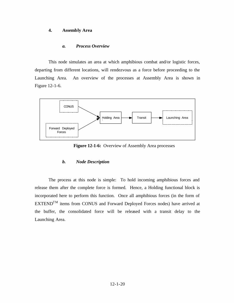
a. Process Overview
This node simulates an area at which amphibious combat and/or logistic forces,
departing from different locations, will rendezvous as a force before proceeding to the
Launching Area. An overview of the processes at Assembly Area is shown in
Figure 12-1-6.
CONUS
Forward DeployedForces
Holding Area Transit Launching Area
Figure 12-1-6: Overview of Assembly Area processes
b. Node Description
The process at this node is simple: To hold incoming amphibious forces and
release them after the complete force is formed. Hence, a Holding functional block is
incorporated here to perform this function. Once all amphibious forces (in the form of
EXTENDTM items from CONUS and Forward Deployed Forces nodes) have arrived at
the buffer, the consolidated force will be released with a transit delay to the
Launching Area.
12-1-21
c. User Setup Requirements
The list of user inputs required at Assembly Area node is as follows:
S/No. Input Description Units of Measure
1. Set required number (or logic inputs) to Holding block —
Table 12-1-6: List of user inputs for Assembly Area node
d. At the Node Input
This node receives Force items from the CONUS and Forward Deployed Forces
nodes.
e. At the Node Output
After all the required Force items have reached the Assembly Area, the Holding
code block will release all the Force items to the Launching Area at its output.
5. Launching Area
a. Process Overview
This is the area where the amphibious force launches the MEB ashore after final
preparation or holding at the Assembly Area. The MEB is launched to their next
destination by employing either the air or sea transporters from the amphibious ships. It
should be noted that transporters are launched based on a schedule planned by the user,
with a loading plan for each wave. An overview of the node is given in Figure 12-1-7.
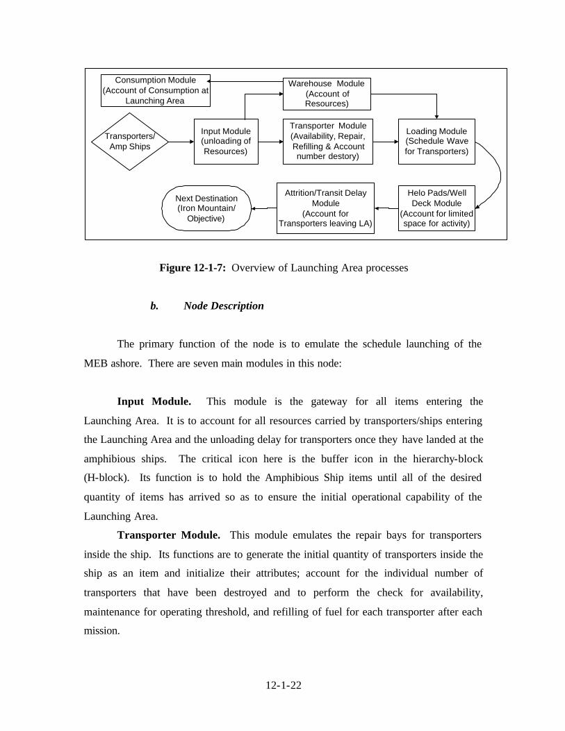
12-1-22
Transporters/Amp Ships
Input Module(unloading ofResources)
Warehouse Module(Account ofResources)
Transporter Module(Availability, Repair,Refilling & Accountnumber destory)
Loading Module(Schedule Wavefor Transporters)
Helo Pads/WellDeck Module
(Account for limitedspace for activity)
Attrition/Transit DelayModule
(Account forTransporters leaving LA)
Next Destination(Iron Mountain/
Objective)
Consumption Module(Account of Consumption at
Launching Area
Figure 12-1-7: Overview of Launching Area processes
b. Node Description
The primary function of the node is to emulate the schedule launching of the
MEB ashore. There are seven main modules in this node:
Input Module. This module is the gateway for all items entering the
Launching Area. It is to account for all resources carried by transporters/ships entering
the Launching Area and the unloading delay for transporters once they have landed at the
amphibious ships. The critical icon here is the buffer icon in the hierarchy-block
(H-block). Its function is to hold the Amphibious Ship items until all of the desired
quantity of items has arrived so as to ensure the initial operational capability of the
Launching Area.
Transporter Module. This module emulates the repair bays for transporters
inside the ship. Its functions are to generate the initial quantity of transporters inside the
ship as an item and initialize their attributes; account for the individual number of
transporters that have been destroyed and to perform the check for availability,
maintenance for operating threshold, and refilling of fuel for each transporter after each
mission.
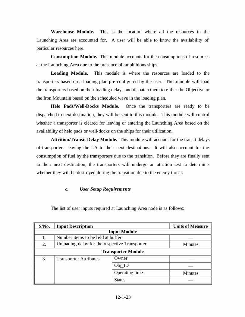
12-1-23
Warehouse Module. This is the location where all the resources in the
Launching Area are accounted for. A user will be able to know the availability of
particular resources here.
Consumption Module. This module accounts for the consumptions of resources
at the Launching Area due to the presence of amphibious ships.
Loading Module. This module is where the resources are loaded to the
transporters based on a loading plan pre-configured by the user. This module will load
the transporters based on their loading delays and dispatch them to either the Objective or
the Iron Mountain based on the scheduled wave in the loading plan.
Helo Pads/Well-Docks Module. Once the transporters are ready to be
dispatched to next destination, they will be sent to this module. This module will control
whether a transporter is cleared for leaving or entering the Launching Area based on the
availability of helo pads or well-docks on the ships for their utilization.
Attrition/Transit Delay Module. This module will account for the transit delays
of transporters leaving the LA to their next destinations. It will also account for the
consumption of fuel by the transporters due to the transition. Before they are finally sent
to their next destination, the transporters will undergo an attrition test to determine
whether they will be destroyed during the transition due to the enemy threat.
c. User Setup Requirements
The list of user inputs required at Launching Area node is as follows:
S/No. Input Description Units of Measure Input Module
1. Number items to be held at buffer — 2. Unloading delay for the respective Transporter Minutes
Transporter Module Owner — Obj_ID — Operating time Minutes
3. Transporter Attributes
Status —
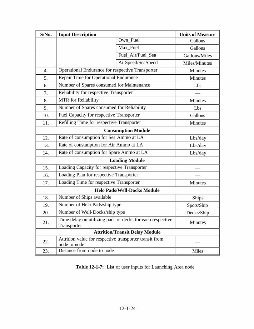
12-1-24
S/No. Input Description Units of Measure Own_Fuel Gallons Max_Fuel Gallons Fuel_Air/Fuel_Sea Gallons/Miles
AirSpeed/SeaSpeed Miles/Minutes 4. Operational Endurance for respective Transporter Minutes 5. Repair Time for Operational Endurance Minutes 6. Number of Spares consumed for Maintenance Lbs 7. Reliability for respective Transporter — 8. MTR for Reliability Minutes 9. Number of Spares consumed for Reliability Lbs 10. Fuel Capacity for respective Transporter Gallons 11. Refilling Time for respective Transporter Minutes
Consumption Module 12. Rate of consumption for Sea Ammo at LA Lbs/day 13. Rate of consumption for Air Ammo at LA Lbs/day 14. Rate of consumption for Spare Ammo at LA Lbs/day
Loading Module 15. Loading Capacity for respective Transporter — 16. Loading Plan for respective Transporter — 17. Loading Time for respective Transporter Minutes
Helo Pads/Well-Docks Module 18. Number of Ships available Ships 19. Number of Helo Pads/ship type Spots/Ship 20. Number of Well-Docks/ship type Decks/Ship
21. Time delay on utilizing pads or decks for each respective Transporter
Minutes
Attrition/Transit Delay Module
22. Attrition value for respective transporter transit from node to node —
23. Distance from node to node Miles
Table 12-1-7: List of user inputs for Launching Area node
12-1-25
d. At the Module input
The inputs to the node will be ships sent from the Assembly Area, the transporters
returning from the Iron Mountain, Beach, or Objective, and air transporters from the
Objective sending the casualties to the Launching Area.
e. At the Module Output
The outputs from the node will be whatever transporters are delivering combat
units and logistic resources.
6. Sea Base
a. Process Overview
The Sea Base is the node where the logistic replenishment ships are based. This
node is present only for the Planned and Conceptual architecture, as the Iron Mountain
plays a similar role in the Current architecture to provide replenishment to the Objective.
This node holds all the resources, vehicles and troops that the MEB requires. It allows
for projection of forces and materials to the Objective, and it also processes demand
requests from the Objective and replenishes the Objective utilizing aircrafts and seacrafts.
The Sea Base node provides accounting of the resources, seacrafts and aircrafts
on the Sea Base ships. It monitors the demand for troops as well as materials by the
Objective, and dynamically loads available seacrafts or aircrafts to fulfill the demands.
The node takes into account loading and unloading times, landing and launching times,
transit times, fuel consumptions and attritions of seacrafts and aircrafts. The node also
accounts for the number of ships at the Sea Base and the available landing spots and
well-docks on each ship. An overview of the interactions between the other nodes and
the Sea Base node is shown in Figure 12-1-8.
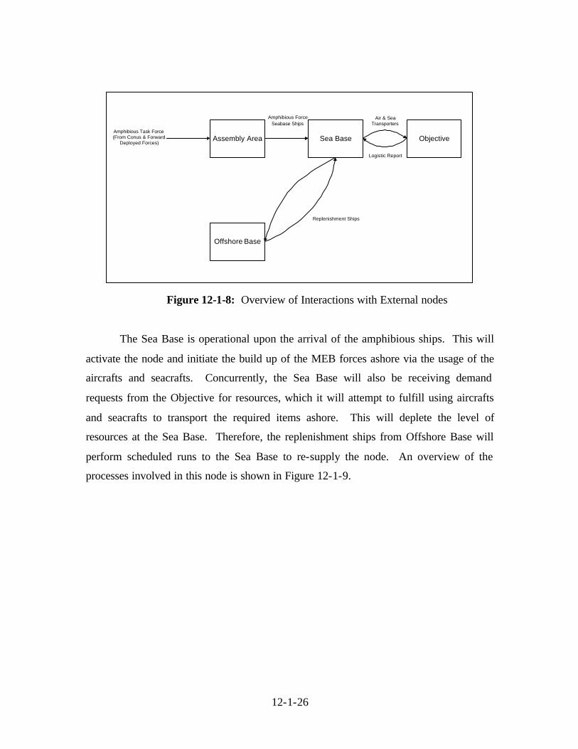
12-1-26
Figure 12-1-8: Overview of Interactions with External nodes
The Sea Base is operational upon the arrival of the amphibious ships. This will
activate the node and initiate the build up of the MEB forces ashore via the usage of the
aircrafts and seacrafts. Concurrently, the Sea Base will also be receiving demand
requests from the Objective for resources, which it will attempt to fulfill using aircrafts
and seacrafts to transport the required items ashore. This will deplete the level of
resources at the Sea Base. Therefore, the replenishment ships from Offshore Base will
perform scheduled runs to the Sea Base to re-supply the node. An overview of the
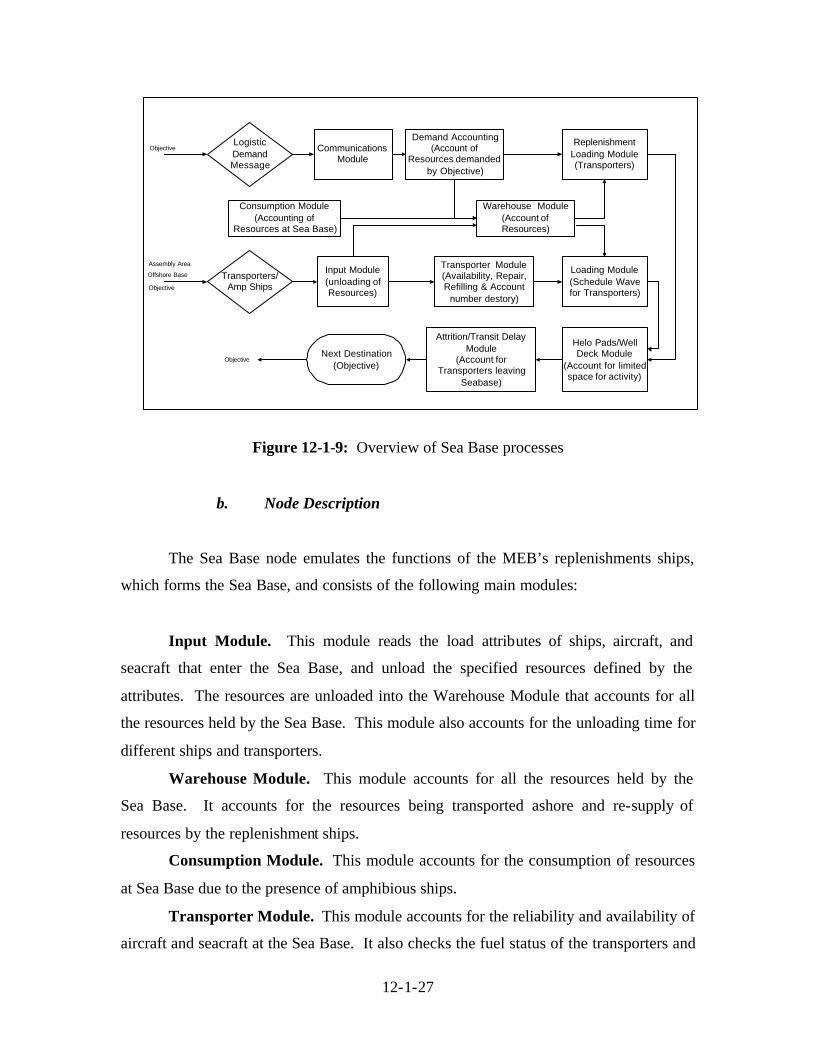
processes involved in this node is shown in Figure 12-1-9.
Assembly Area
Offshore Base
Sea Base Objective
Amphibious ForceSeabase Ships
Replenishment Ships
Air & SeaTransporters
Amphibious Task Force(From Conus & Forward
Deployed Forces)
Logistic Report
12-1-27
Transporters/Amp Ships
Input Module(unloading ofResources)
Warehouse Module(Account ofResources)
Transporter Module(Availability, Repair,Refilling & Account
number destory)
Loading Module(Schedule Wavefor Transporters)
Helo Pads/WellDeck Module
(Account for limitedspace for activity)
Attrition/Transit DelayModule
(Account forTransporters leaving
Seabase)
Next Destination(Objective)
LogisticDemandMessage
Demand Accounting(Account of
Resources demandedby Objective)
ReplenishmentLoading Module(Transporters)
Objective
Assembly Area
Objective
Offshore Base
Objective
CommunicationsModule
Consumption Module(Accounting of
Resources at Sea Base)
Figure 12-1-9: Overview of Sea Base processes
b. Node Description
The Sea Base node emulates the functions of the MEB’s replenishments ships,
which forms the Sea Base, and consists of the following main modules:
Input Module. This module reads the load attributes of ships, aircraft, and
seacraft that enter the Sea Base, and unload the specified resources defined by the
attributes. The resources are unloaded into the Warehouse Module that accounts for all
the resources held by the Sea Base. This module also accounts for the unloading time for
different ships and transporters.
Warehouse Module. This module accounts for all the resources held by the
Sea Base. It accounts for the resources being transported ashore and re-supply of
resources by the replenishment ships.
Consumption Module. This module accounts for the consumption of resources
at Sea Base due to the presence of amphibious ships.
Transporter Module. This module accounts for the reliability and availability of
aircraft and seacraft at the Sea Base. It also checks the fuel status of the transporters and
12-1-28
refills them as necessary. This module also accounts for the number of transporters that
are out-of-action.
Loading Module. This module projects the MEB ashore using a pre-planned
schedule. The schedule specifies the waves and composition of forces to be carried by
individual transporters in order to mimic an actual build-up plan. Resources are loaded
from the Warehouse Module onto the transporters, and then sent to the Objective.
Helo Pads/Well-Dock Module. This module models the landing and taking off
of the aircrafts, as well as the launching of the seacraft. It models the characteristics of
the different amphibious ships at the Sea Base, e.g., the number of helicopter landing
spots and well-docks available on each ship. Hence, the total number of launching
platforms put an upper availability limit for both the aircraft and seacraft at any point in
time.
Attrition/Transit Delay Module. This module calculates the time that individual
transporters will spent in transit to the Objective. It also accounts for the fuel that the
transporters consumes and logs it within the attributes of the transporters. It also
determines whether each individual transporter will be out-of-action according to a
user-defined attrition probability.
Communications Module. This module establishes communications between
the Sea Base and the Objective for logistic requests from the Objective, in order for the
Sea Base to send the required replenishments.
Demand Accounting Module. This module accounts for the demand by the
Objective that was sent through the Communications Module. It also decides, based on
user-inputted thresholds, whether and when to send the resources to the Objective.
Replenishment Loading Module. This module receives information from the
Demand Accounting Module on what type of resources to send to the Objective. It
calculates the amount of resources and selects the transport available to send the
resources ashore. This module also accounts for the resources being depleted, taking
them from the Warehouse Module and then sending them to the Objective.
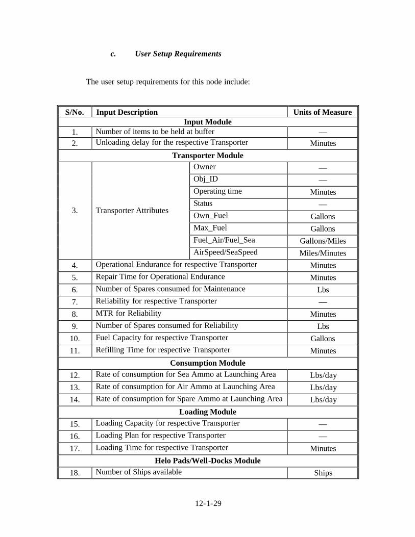
12-1-29
c. User Setup Requirements
The user setup requirements for this node include:
S/No. Input Description Units of Measure Input Module
1. Number of items to be held at buffer — 2. Unloading delay for the respective Transporter Minutes
Transporter Module Owner — Obj_ID — Operating time Minutes Status — Own_Fuel Gallons Max_Fuel Gallons Fuel_Air/Fuel_Sea Gallons/Miles
3. Transporter Attributes
AirSpeed/SeaSpeed Miles/Minutes 4. Operational Endurance for respective Transporter Minutes 5. Repair Time for Operational Endurance Minutes 6. Number of Spares consumed for Maintenance Lbs 7. Reliability for respective Transporter — 8. MTR for Reliability Minutes 9. Number of Spares consumed for Reliability Lbs 10. Fuel Capacity for respective Transporter Gallons 11. Refilling Time for respective Transporter Minutes
Consumption Module 12. Rate of consumption for Sea Ammo at Launching Area Lbs/day 13. Rate of consumption for Air Ammo at Launching Area Lbs/day 14. Rate of consumption for Spare Ammo at Launching Area Lbs/day
Loading Module 15. Loading Capacity for respective Transporter — 16. Loading Plan for respective Transporter — 17. Loading Time for respective Transporter Minutes
Helo Pads/Well-Docks Module 18. Number of Ships available Ships
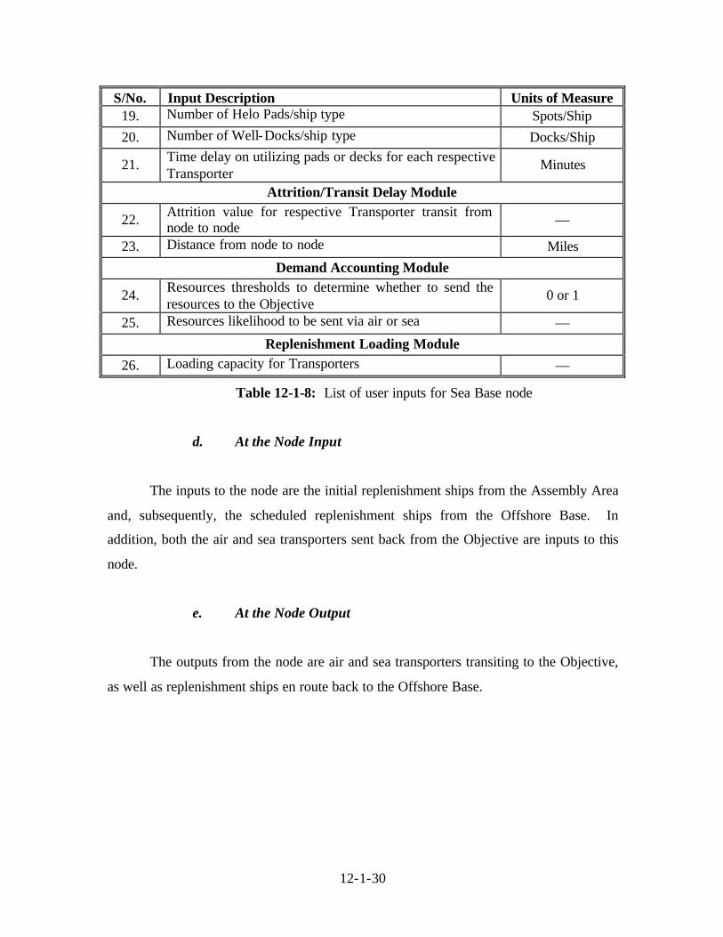
12-1-30
S/No. Input Description Units of Measure 19. Number of Helo Pads/ship type Spots/Ship 20. Number of Well-Docks/ship type Docks/Ship
21. Time delay on utilizing pads or decks for each respective Transporter
Minutes
Attrition/Transit Delay Module
22. Attrition value for respective Transporter transit from node to node —
23. Distance from node to node Miles Demand Accounting Module
24. Resources thresholds to determine whether to send the resources to the Objective
0 or 1
25. Resources likelihood to be sent via air or sea — Replenishment Loading Module
26. Loading capacity for Transporters —
Table 12-1-8: List of user inputs for Sea Base node
d. At the Node Input
The inputs to the node are the initial replenishment ships from the Assembly Area
and, subsequently, the scheduled replenishment ships from the Offshore Base. In
addition, both the air and sea transporters sent back from the Objective are inputs to this
node.
e. At the Node Output
The outputs from the node are air and sea transporters transiting to the Objective,
as well as replenishment ships en route back to the Offshore Base.
12-1-31
7. Beach
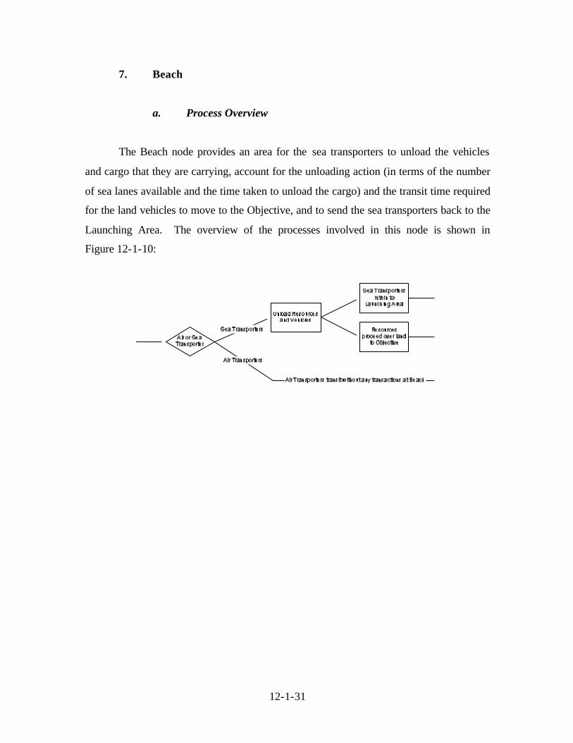
a. Process Overview
The Beach node provides an area for the sea transporters to unload the vehicles
and cargo that they are carrying, account for the unloading action (in terms of the number
of sea lanes available and the time taken to unload the cargo) and the transit time required
for the land vehicles to move to the Objective, and to send the sea transporters back to the
Launching Area. The overview of the processes involved in this node is shown in
Figure 12-1-10:
Figure 12-1-10: Overview of Beach processes
b. Node Description
The major modules in this node are Unload Resources and
Transit Delay/Consumption of Resources.
Unload Resource Module. In the Unload Resources Module, the Marines,
water, ground ammunition, fuel, food, and all vehicles carried by the transporter will be
unloaded and sent to the Objective. The transporter will also be delayed at this module
according to its unloading time and the number of transporters allowed to perform this
action will be limited by the number of sea lanes available.
Transit Delay/Consumption of Resource Module. For the
Transit Delay/Consumption of Resources Module, the transporter will be held at this
12-1-32
module based on the transit time (calculated by the distance divided by its speed) and its
operating fuel deducted by the amount needed to reach the next destination (calculated by
the distance divided by its rate of fuel consumption). As noted previously, air
transporters are identified and sent directly to the Objective, as they do not perform any
processes at the beach.
c. User Setup Requirements
The user setup requirements for this node include:
S/No. Input Description Units of Measure 1. Number of sea lanes available — 2. Unloading delay for the various types of sea
transports Minutes
3. Vehicle attributes (each set of every vehicle): Speed Rate of fuel consumption Fuel capacity
Miles/hour
Gallons/mile Gallons
4. Distance between Beach and Launching Area Nautical Miles 5. Distance between Beach and Objective Miles
Table 12-1-9: List of user inputs for Beach node
d. Node Input
The inputs to the node will be both air and sea transporters sent from the
Launching Area.
e. Node Output
The outputs from the node will be sea transporters returning to the
Launching Area and air and ground transporters transiting to the Objective.
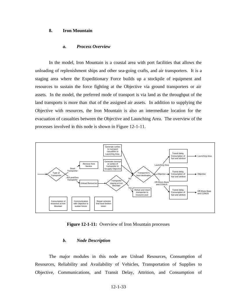
12-1-33
8. Iron Mountain
a. Process Overview
In the model, Iron Mountain is a coastal area with port facilities that allows the
unloading of replenishment ships and other sea-going crafts, and air transporters. It is a
staging area where the Expeditionary Force builds up a stockpile of equipment and
resources to sustain the force fighting at the Objective via ground transporters or air
assets. In the model, the preferred mode of transport is via land as the throughput of the
land transports is more than that of the assigned air assets. In addition to supplying the
Objective with resources, the Iron Mountain is also an intermediate location for the
evacuation of casualties between the Objective and Launching Area. The overview of the
processes involved in this node is shown in Figure 12-1-11.
Type ofTransporter
Unload Resources
Air/Land/SeaTransporter
Remove fromService
DeadTransporter
Transporterstaying at Iron
Mountain
Refuel and returntransporter toresource pool
Yes
Transporter'sNext destination
No
Transit delay,Consumption offuel and attrition
Transit delay,Consumption offuel and attrition
Transit delay,Consumption offuel and attrition
Launching Area
Objective
Off-Shore Baseand CONUS
Launching Area
Objective
Off-Shore Baseand CONUS
Consumption ofresources at Iron
Mountain
Communicationwith Objective to
sustain forces
Repair vehiclesthat have broken
down
Generate convoysor sorties of
transporter toresupply Objective
Generate sortiesto transport
casualties toLaunching Area
Figure 12-1-11: Overview of Iron Mountain processes
b. Node Description
The major modules in this node are Unload Resources, Consumption of
Resources, Reliability and Availability of Vehicles, Transportation of Supplies to
Objective, Communications, and Transit Delay, Attrition, and Consumption of
12-1-34
Transporter Resources. Some of these modules interact with each other by passing
information and resources, while others perform their roles in isolation. Items that come
into and out of the Iron Mountain node are transporters (vehicles, sea-going vessels, and
aircraft) and communication messages. Casualties that originate from the Objective will
be transported back to the Iron Mountain. Once there, they will be evacuated out to the
Launching Area by air transporters held at the Iron Mountain.
Unload Resources Module. When a transporter first arrives at the node, its
attributes will be read to determine its identity. Transporters that have been attrited will
be removed from the model while ground, air, and sea-going transporters will be routed
to the Unload Resources Module. In the Unload Resources Module, the number of air
transporters that are allowed to unload their resources will be restricted by the number of
landing spots; while the number of sea-going transporters (less those that dock along the
port) will be restricted by the number of sea lanes available. The troops, casualties,
water, ground ammunition, fuel, food, and all vehicles carried by the transporters will be
unloaded and stored at the Iron Mountain node. The transporters will also be delayed at
this module according to their unloading time.
Once a transporter finishes unloading its resources its attributes will be read again
to determine if the transporter will report to the Iron Mountain node for duty or be
returned to its originating node for other duties. Transporters remaining at the
Iron Mountain node will be refueled and stored while those leaving the Iron Mountain
node will proceed to the Transit Delay, Attrition and Consumption of Resources module.
Transit Delay, Attrition, and Consumption of Transporter Resources
Module. In the Transit Delay, Attrition, and Consumption of Transporter Resources
Module, the transporter will be held in this module based on the transit time (calculated
by the distance divided by its speed) and its operating fuel deducted by the amount
needed to reach the next destination (calculated by the distance divided by its rate of fuel
consumption). The rate of attrition will also determine if the transporter will be
destroyed during the transit to its next destination. Attrited transporters will be sent back
to their originating node so that they can be removed from the model.
Consumption of Resources Module. Once the Expeditionary Force occupies the
Iron Mountain, it begins to consume the resources that are held there in the Consumption
12-1-35
of Resources Module. The amount of food, water, ground ammunition, air ammunition,
fuel, and spares will be deducted from the resources on a daily basis, based on a
pre-determined consumption rate. Attrition of Marines and generation of casualties also
occur on a daily basis, based on the attrition rate for the Iron Mountain.
Reliability and Availability of Vehicles Module. Vehicles stored at the
Iron Mountain node are subjected to reliability constraints through the Reliability and
Availability of Vehicles Module. In this module, vehicles are removed from the resource
pool based on their respective reliability rates for an interval of 24 hours (to simulate the
repair of said vehicles) before they are released back into the resource pool. Vehicles
taken out of service will not be made available for any missions or re-supply until they
are returned back to the resource pool.
Communications Module. Communication messages that arrive from the
Objective will be routed to the Communications Module. In the model, communications
between the Objective and Iron Mountain nodes exist to facilitate the supply process.
Every eight hours, Objective will send a message to Iron Mountain, requesting for
resources that have been depleted. In the Communications Module, the message will be
decoded and the amount of each resource (i.e., troops, ground ammunition, water, fuel,
combat vehicles) requested by Objective will be stored. The Communications Module
will then initiate the supply process by triggering a demand for transporters or combat
vehicles to report to the Objective. In this supply process, the primary means is to deliver
the resources using ground transporters (trucks and HMMWVs). Similarly, ground
combat vehicles, with the exception of the M198 howitzer, will move independently to
the Objective based on the number of each vehicles requested. The supply of M198
howitzers to the Objective will only occur if there are trucks available to tow the howitzer
to the Objective. Besides the ground transporters, air transporters can also transport the
mission-critical resources (i.e., water, fuel, food, and ground ammunition) to the
Objective. Once the resources leave the Iron Mountain node, the Objective request
stored will be deducted to reflect the completion of the entire communication and supply
process.
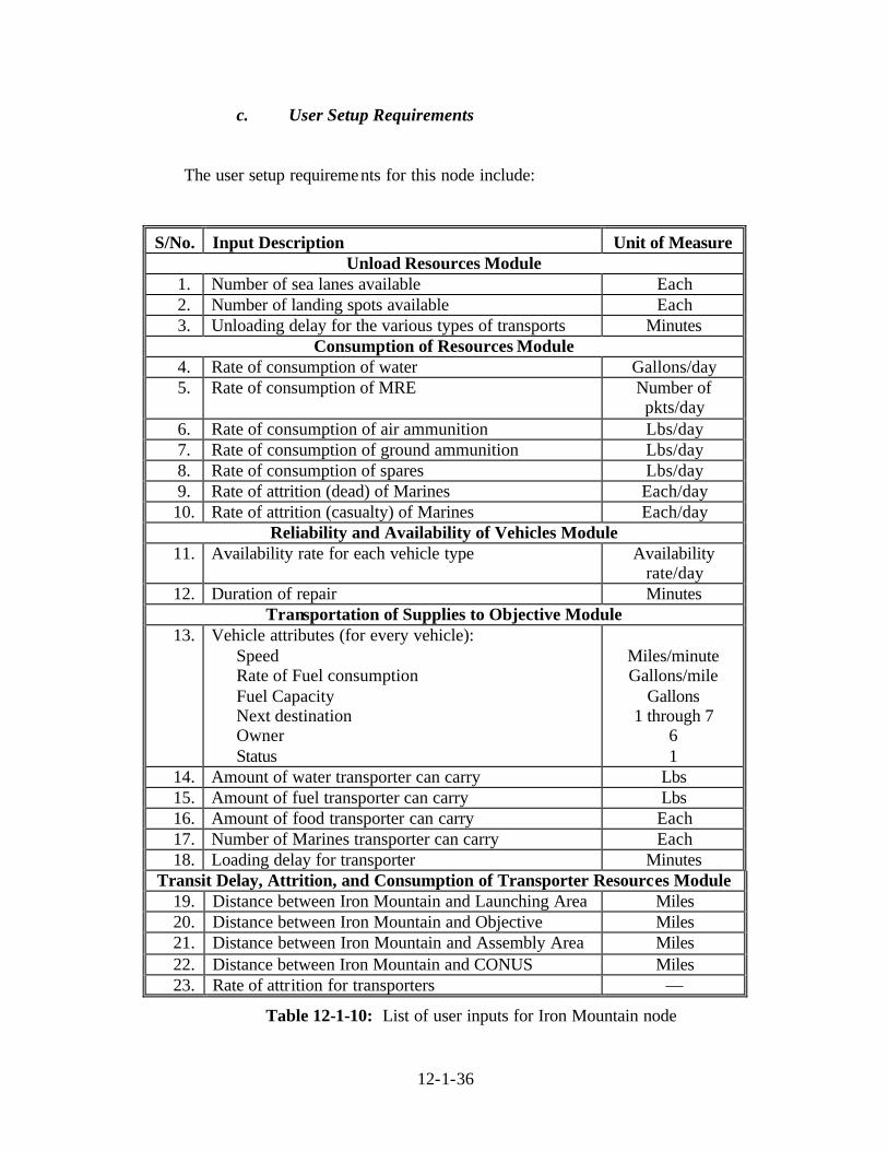
12-1-36
c. User Setup Requirements
The user setup requirements for this node include:
S/No. Input Description Unit of Measure Unload Resources Module
1. Number of sea lanes available Each 2. Number of landing spots available Each 3. Unloading delay for the various types of transports Minutes
Consumption of Resources Module 4. Rate of consumption of water Gallons/day 5. Rate of consumption of MRE Number of
pkts/day 6. Rate of consumption of air ammunition Lbs/day 7. Rate of consumption of ground ammunition Lbs/day 8. Rate of consumption of spares Lbs/day 9. Rate of attrition (dead) of Marines Each/day 10. Rate of attrition (casualty) of Marines Each/day
Reliability and Availability of Vehicles Module 11. Availability rate for each vehicle type Availability
rate/day 12. Duration of repair Minutes
Transportation of Supplies to Objective Module 13. Vehicle attributes (for every vehicle):
Speed Rate of Fuel consumption Fuel Capacity Next destination Owner Status
Miles/minute Gallons/mile
Gallons 1 through 7
6 1
14. Amount of water transporter can carry Lbs 15. Amount of fuel transporter can carry Lbs 16. Amount of food transporter can carry Each 17. Number of Marines transporter can carry Each 18. Loading delay for transporter Minutes
Transit Delay, Attrition, and Consumption of Transporter Resources Module 19. Distance between Iron Mountain and Launching Area Miles 20. Distance between Iron Mountain and Objective Miles 21. Distance between Iron Mountain and Assembly Area Miles 22. Distance between Iron Mountain and CONUS Miles 23. Rate of attrition for transporters —
Table 12-1-10: List of user inputs for Iron Mountain node
12-1-37
d. At the Node Input
The inputs to the node include air and sea transporters from the Launching Area
node, sea transporters from the Assembly Area and Off-Shore Base nodes, and ground
transporters from the Objective node. Communication messages will also be sent into the
node from the Objective node.
e. At the Node Output
The outputs from the node will be air and sea transporters returning to the
Launching Area, sea transporters to the CONUS and Off-Shore Base nodes, and ground
transporters to the Objective node. Communication messages will also be sent to the
Objective node. The status of the primary resources (food, fuel, and ground ammunition)
held at the Iron Mountain node will also be recorded for further analysis.
9. Objective
a. Process Overview
In the model, the Objective is a target area that the Expeditionary Force intends to
capture. The Objective can be as far inland as 200 nautical miles (NM) and the
Expeditionary Force is expected to be able to fight and sustain itself for up to 15 days
with its organic assets, and indefinitely when augmented with Maritime Pre-positioned
Force assets. The overview of the processes involved in this node is shown in
Figure 12-1-12.
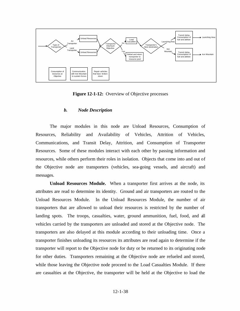
12-1-38
Type ofTransporter
Transporterstaying atObjective
Refuel and returntransporter toresource pool
Yes
Transporter'sNext destination
No
Transit delay,Consumption offuel and attrition
Transit delay,Consumption offuel and attrition
Launching Area
IronMountain
Launching Area
Iron Mountain
Consumption ofresources at
Objective
Communicationwith Iron Mountainto sustain forces
Repair vehiclesthat have broken
down
LandTransporter
Unload Resources
Unload ResourcesAir
Transporter
LoadCasualties
Figure 12-1-12: Overview of Objective processes
b. Node Description
The major modules in this node are Unload Resources, Consumption of
Resources, Reliability and Availability of Vehicles, Attrition of Vehicles,
Communications, and Transit Delay, Attrition, and Consumption of Transporter
Resources. Some of these modules interact with each other by passing information and
resources, while others perform their roles in isolation. Objects that come into and out of
the Objective node are transporters (vehicles, sea-going vessels, and aircraft) and
messages.
Unload Resources Module. When a transporter first arrives at the node, its
attributes are read to determine its identity. Ground and air transporters are routed to the
Unload Resources Module. In the Unload Resources Module, the number of air
transporters that are allowed to unload their resources is restricted by the number of
landing spots. The troops, casualties, water, ground ammunition, fuel, food, and all
vehicles carried by the transporters are unloaded and stored at the Objective node. The
transporters are also delayed at this module according to their unloading time. Once a
transporter finishes unloading its resources its attributes are read again to determine if the
transporter will report to the Objective node for duty or be returned to its originating node
for other duties. Transporters remaining at the Objective node are refueled and stored,
while those leaving the Objective node proceed to the Load Casualties Module. If there
are casualties at the Objective, the transporter will be held at the Objective to load the
12-1-39
casualties so that they can be evacuated for further treatment. The delay time for each
transporter is dependent on the number of casualties that it can carry. Once the
transporter is done loading the casualties, it is sent to the Transit Delay, Attrition, and
Consumption of Transporter Resources Module.
Transit Delay, Attrition, and Consumption of Transporter Resources
Module. In the Transit Delay, Attrition, and Consumption of Transporter Resources
Module, the transporter is held based on the transit time (calculated by the distance
divided by its speed) and its operating fuel deducted by the amount needed to reach the
next destination (calculated by the distance divided by its rate of fuel consumption). The
rate of attrition also determines if the transporter will be out-of-action during the transit to
its next destination. Attrited transporters are sent back to their originating node so that
they can be removed from the model. Besides availability and reliability, vehicles at the
Objective are also subjected to attrition by enemy action in the Attrition module. At the
end of each day, the vehicles held at the Objective node are reduced by the attrition rate
determined by the user. These vehicles are taken out of the model and do not interact
with the model in any other way (i.e., there is no simulation of the salvage process for
damaged or destroyed vehicles).
Consumption of Resources Module. Once the Expeditionary Force occupies the
Objective, it begins to consume the resources that are held there in the Consumption of
Resources Module. The amount of food, water, ground ammunition, air ammunition,
fuel, and spares are deducted from the resources on a daily basis, based on a
pre-determined consumption rate. Attrition of Marines and generation of casualties also
occur on a daily basis, based on the attrition rate for the Objective.
Reliability and Availability of Vehicles Module. Vehicles stored at the
Objective node are subjected to reliability constraints through the Reliability and
Availability of Vehicles Module. In this module, vehicles are removed from the resource
pool based on their respective reliability rates for an interval of 24 hours (to simulate the
repair of the vehicles) before they are released back into the resource pool. Vehicles
taken out of service are not made available for any missions or re-supply until they are
returned back to the resource pool.
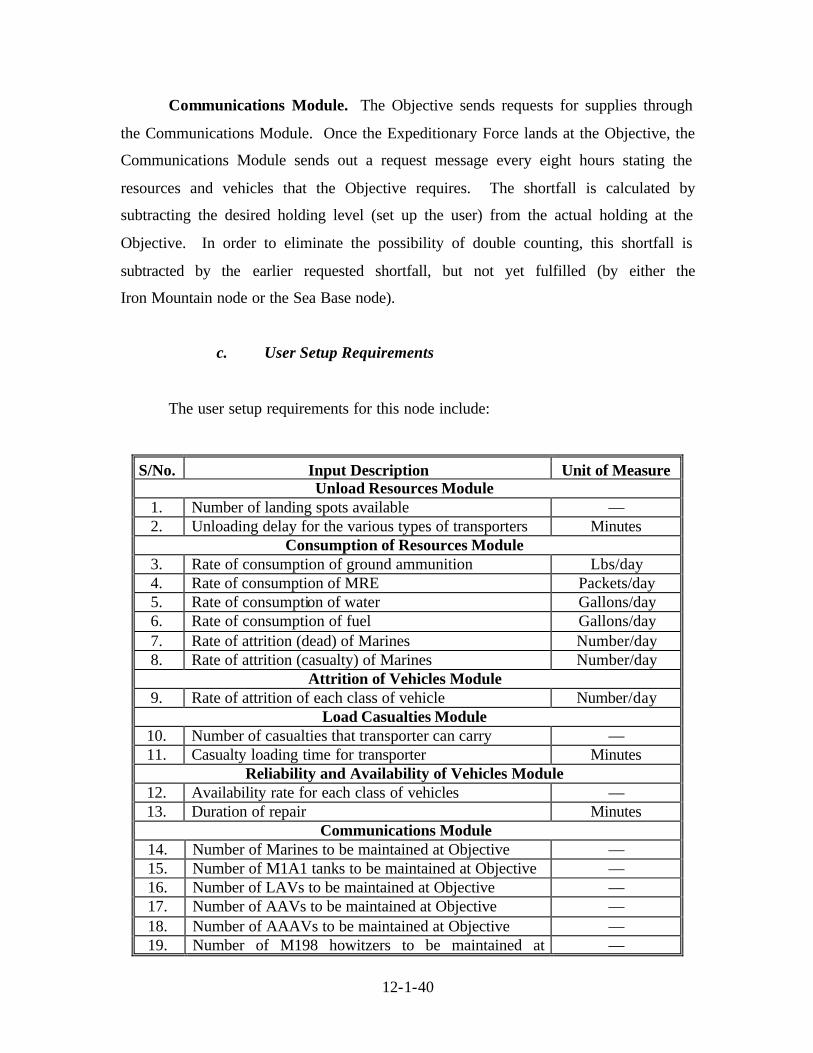
12-1-40
Communications Module. The Objective sends requests for supplies through
the Communications Module. Once the Expeditionary Force lands at the Objective, the
Communications Module sends out a request message every eight hours stating the
resources and vehicles that the Objective requires. The shortfall is calculated by
subtracting the desired holding level (set up the user) from the actual holding at the
Objective. In order to eliminate the possibility of double counting, this shortfall is
subtracted by the earlier requested shortfall, but not yet fulfilled (by either the
Iron Mountain node or the Sea Base node).
c. User Setup Requirements
The user setup requirements for this node include:
S/No. Input Description Unit of Measure Unload Resources Module
1. Number of landing spots available — 2. Unloading delay for the various types of transporters Minutes
Consumption of Resources Module 3. Rate of consumption of ground ammunition Lbs/day 4. Rate of consumption of MRE Packets/day 5. Rate of consumption of water Gallons/day 6. Rate of consumption of fuel Gallons/day 7. Rate of attrition (dead) of Marines Number/day 8. Rate of attrition (casualty) of Marines Number/day
Attrition of Vehicles Module 9. Rate of attrition of each class of vehicle Number/day
Load Casualties Module 10. Number of casualties that transporter can carry — 11. Casualty loading time for transporter Minutes
Reliability and Availability of Vehicles Module 12. Availability rate for each class of vehicles — 13. Duration of repair Minutes
Communications Module 14. Number of Marines to be maintained at Objective — 15. Number of M1A1 tanks to be maintained at Objective — 16. Number of LAVs to be maintained at Objective — 17. Number of AAVs to be maintained at Objective — 18. Number of AAAVs to be maintained at Objective — 19. Number of M198 howitzers to be maintained at —
12-1-41
S/No. Input Description Unit of Measure Objective
20. Number of HMMWVs to be maintained at Objective — 21. Number of trucks to be maintained at Objective — 22. Number of packets of MREs to be maintained at
Objective —
23. Amount of fuel to be maintained at Objective Gallons 24. Amount of ground ammunition to be maintained at
Objective Pounds
25. Amount of water to be maintained at Objective Gallons 26. Interval between messages Minutes
Transit Delay, Attrition, and Consumption of Transporter Resources Module 27. Distance between Objective and Launching Area Miles 28. Distance between Objective and Iron Mountain Miles 29. Distance between Objective and Assembly Area Miles 30. Rate of attrition for transporters —
Table 12-1-11: List of user inputs for Objective node
d. Node Input
The inputs to the node include air and sea transporters from the Launching Area
node, sea transporters from the Assembly Area and Off-Shore Base nodes, and ground
transporters from the Objective node. Communication messages are also sent into the
node from the Objective node.
e. Node Output
The outputs from the node are air transporters returning to the Launching Area
and ground transporters to the Iron Mountain node. Communication messages are also
sent to the Iron Mountain node. The status of the primary resources (food, water, fuel,
and ground ammunition), the number of each combat force element (M1A1 tanks, LAVs,
AAVs, AAAVs, M198 howitzers, HMMWVs, and troops) held at the Objective node are
also recorded for further analysis.
12-1-42
F. PRE-SIMULATION SETUP
We created three variants of the ExWar EXTENDTM Model to represent for the
Current, Planned, and Conceptual architectures, respectively. Hence, the appropriate
variant of the model would need to be used correctly depending on the architecture
desired. With the user input file that was created for the ExWar Model, it is necessary to
make the appropriate settings and key in data at each node as the initial state of the
model. As the ExWar Model is an extensive and complex model, we aggregated most of
the code blocks into H-blocks for easy re-use and presentation at the top level. Hence, it
is necessary to enter those H-blocks to make the settings and data entry. In addition,
there are two text files that would hold information pertaining to transporter preference
for the air and ground transportation in the Launching Area node. These two files have to
be in the same folder as the EXTENDTM Model code file on the computer. Otherwise,
when executed, the simulation software would return an error message.
On completion of model settings and data entry, it is necessary to make settings in
the EXTENDTM program itself. Firstly, the global time step has to be defined. For our
study, we wished to study the processes in the resolution of time steps of minutes.
Hence, the global time units under “simulation setup” was set to “minutes.” This is the
default time unit for all blocks that use “default” as their time units. Hence, for new code
blocks that were added subsequently, extra care had to be exercised to ensure the correct
time units were chosen. Depending on the length of time desired to investigate the
ExWar processes, it was also necessary to set the simulation end time. In the case of our
study, we set this to end at 90 days. If variability were also being used in the model,
other settings in the “simulation setup” would also be necessary.
G. MODEL OUTPUTS
The EXTENDTM software allows us to derive outputs in many formats. It is
possible to write the outputs to a text file, generate graphs from the plotter utilities, or
export entire tables out to another application (e.g., the spreadsheet program Excel) for
further processing. In addition, there are dialogue boxes in certain code blocks, which
12-1-43
may provide relevant information (such as average queue length, average wait time, etc.)
that may be of importance for further analysis to be done.
In the ExWar Model, we decided that we would use the plotters to record the
Combat Power Index (CPI) at the Objective. This index uses the number of each entity
(troops, M1A1 tanks, LAVs, etc.) multiplied by their respective CPI to generate an
aggregated CPA at the Objective at any specific point in time. To assist us in the analysis
of the CPA, we have also recorded the number of troops, M1A1 tanks, LAVs, trucks,
HMMWVs, M198 howitzers, AAVs, and AAAVs that are held at the Objective at times
during each model run.
Besides the CPA, we also monitored the status of the logistics supplies held at the
Iron Mountain/Sea Base and the Objective. At the Objective, the amount of water, food,
ground ammunition, and fuel held is recorded. At the Iron Mountain/Sea Base, only the
amount of fuel, food, and ground ammunition held is recorded. Water was not included
as our assumption was that the Iron Mountain/Sea Base would generate the water needed
to supply the Objective.
The raw outputs from EXTENDTM were processed with Excel to generate the
results that facilitated our analysis. For the CPA, a threshold was set to determine the
time at which this limit was breached. For the logistics supplies, the raw data was
converted to show the number of days of supply that each of the nodes held instead of
just how much of each supply the node held. From there, we determined the average
deviation of the supplies held at the node versus the targeted profile for the analysis of the
outputs.

APPENDIX 12-2
Attrition Rate Vis-À-Vis Probabilistic Attrition
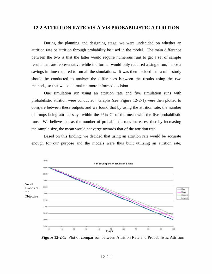
12-2-1
12-2 ATTRITION RATE VIS-À-VIS PROBABILISTIC ATTRITION
During the planning and designing stage, we were undecided on whether an
attrition rate or attrition through probability be used in the model. The main difference
between the two is that the latter would require numerous runs to get a set of sample
results that are representative while the formal would only required a single run, hence a
savings in time required to run all the simulations. It was then decided that a mini-study
should be conducted to analyze the differences between the results using the two
methods, so that we could make a more informed decision.
One simulation run using an attrition rate and five simulation runs with
probabilistic attrition were conducted. Graphs (see Figure 12-2-1) were then plotted to
compare between these outputs and we found that by using the attrition rate, the number
of troops being attrited stays within the 95% CI of the mean with the five probabilistic
runs. We believe that as the number of probabilistic runs increases, thereby increasing
the sample size, the mean would converge towards that of the attrition rate.
Based on this finding, we decided that using an attrition rate would be accurate
enough for our purpose and the models were thus built utilizing an attrition rate.
Figure 12-2-1: Plot of comparison between Attrition Rate and Probabilistic Attrition
Days
No. of Troops at the Objective
APPENDIX 12-3
Validation of Models Data
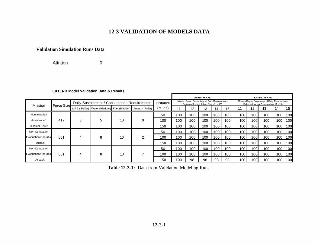
12-3-1
12-3 VALIDATION OF MODELS DATA
Validation Simulation Runs Data
Table 12-3-1: Data from Validation Modeling Runs
Attrition 0
EXTEND Model Validation Data & Results
MRE ( Pallet) Water (Bladder) Fuel (Bladder) Ammo - (Pallet) 11 12 13 14 15 11 12 13 14 15
Humanitarian 50 100 100 100 100 100 100 100 100 100 100Assistance/ 100 100 100 100 100 100 100 100 100 100 100
Disaster Relief 150 100 100 100 100 100 100 100 100 100 100Non-Combatant 50 100 100 100 100 100 100 100 100 100 100
Evacuation Operation 651 4 8 10 2 100 100 100 100 100 100 100 100 100 100 100 - Sustain 150 100 100 100 100 100 100 100 100 100 100
Non-Combatant 50 100 100 100 100 100 100 100 100 100 100 Evacuation Operation 651 4 8 10 7 100 100 100 100 100 100 100 100 100 100 100
- Assault 150 100 98 96 93 93 100 100 100 100 100
ARENA MODEL EXTEND MODEL
Mission Force SizeDaily Sustainment / Consumption Requirements Distance
(Miles)
Mission Days - Percentage of Daily Requirements Delivered for last 5 days (days 11 - 15)
Mission Days - Percentage of Daily Requirements Delivered for last 5 days (days 11 - 15)
0417 3 5 10

APPENDIX 12-4
User Input Data
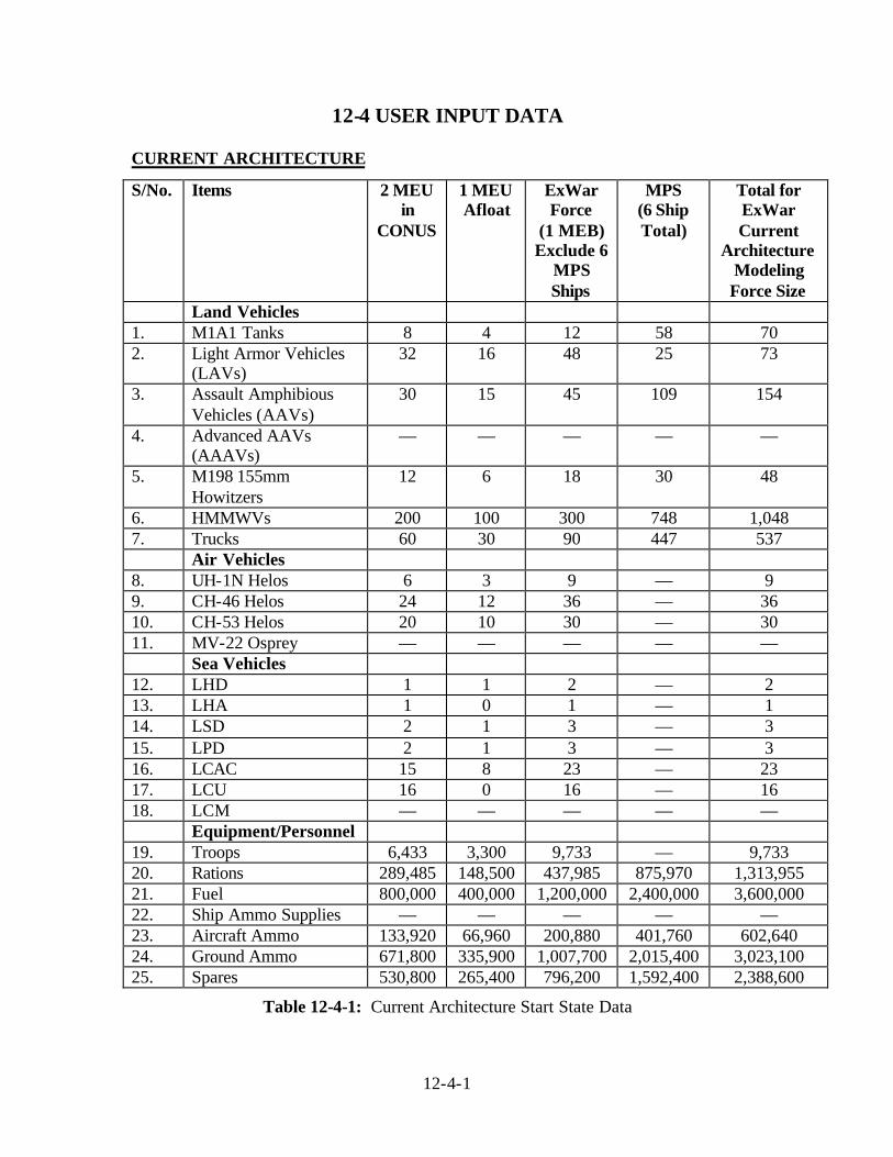
12-4-1
12-4 USER INPUT DATA
CURRENT ARCHITECTURE
S/No. Items 2 MEU in
CONUS
1 MEU Afloat
ExWar Force
(1 MEB) Exclude 6
MPS Ships
MPS (6 Ship Total)
Total for ExWar Current
Architecture Modeling Force Size
Land Vehicles 1. M1A1 Tanks 8 4 12 58 70 2. Light Armor Vehicles
(LAVs) 32 16 48 25 73
3. Assault Amphibious Vehicles (AAVs)
30 15 45 109 154
4. Advanced AAVs (AAAVs)
— — — — —
5. M198 155mm Howitzers
12 6 18 30 48
6. HMMWVs 200 100 300 748 1,048 7. Trucks 60 30 90 447 537 Air Vehicles 8. UH-1N Helos 6 3 9 — 9 9. CH-46 Helos 24 12 36 — 36 10. CH-53 Helos 20 10 30 — 30 11. MV-22 Osprey — — — — — Sea Vehicles 12. LHD 1 1 2 — 2 13. LHA 1 0 1 — 1 14. LSD 2 1 3 — 3 15. LPD 2 1 3 — 3 16. LCAC 15 8 23 — 23 17. LCU 16 0 16 — 16 18. LCM — — — — — Equipment/Personnel 19. Troops 6,433 3,300 9,733 — 9,733 20. Rations 289,485 148,500 437,985 875,970 1,313,955 21. Fuel 800,000 400,000 1,200,000 2,400,000 3,600,000 22. Ship Ammo Supplies — — — — — 23. Aircraft Ammo 133,920 66,960 200,880 401,760 602,640 24. Ground Ammo 671,800 335,900 1,007,700 2,015,400 3,023,100 25. Spares 530,800 265,400 796,200 1,592,400 2,388,600
Table 12-4-1: Current Architecture Start State Data
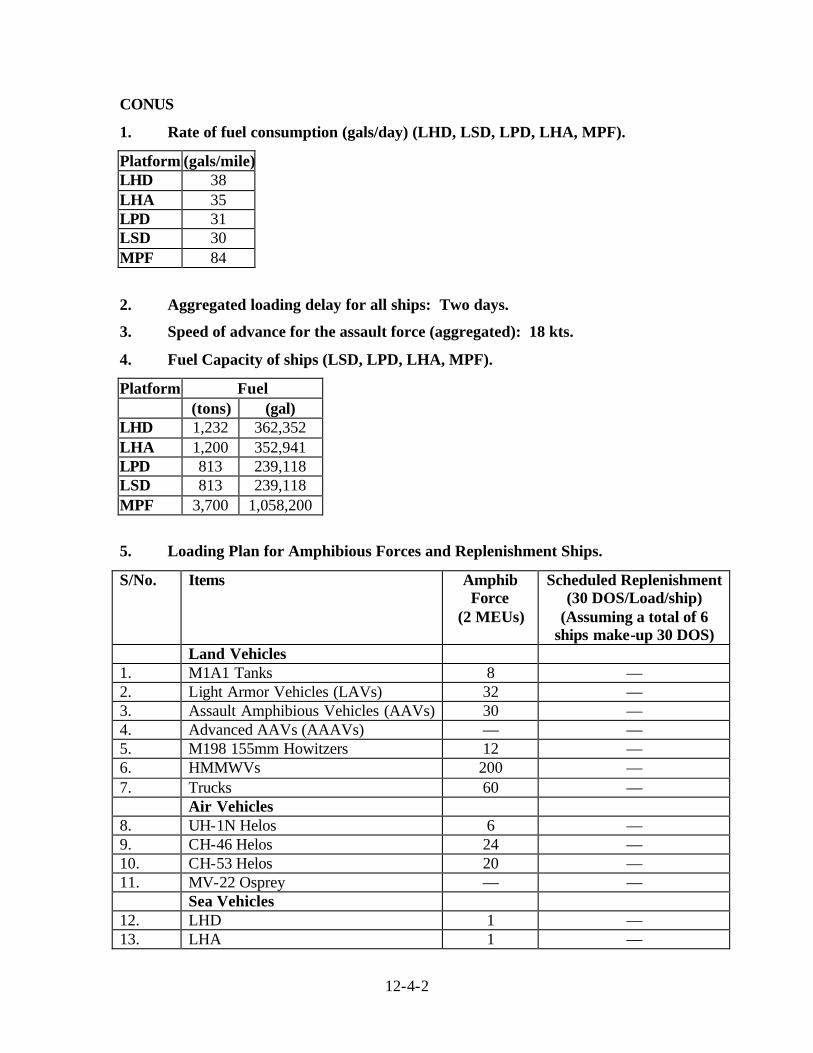
12-4-2
CONUS
1. Rate of fuel consumption (gals/day) (LHD, LSD, LPD, LHA, MPF).
Platform (gals/mile)LHD 38 LHA 35 LPD 31 LSD 30 MPF 84
2. Aggregated loading delay for all ships: Two days.
3. Speed of advance for the assault force (aggregated): 18 kts.
4. Fuel Capacity of ships (LSD, LPD, LHA, MPF).
Platform Fuel (tons) (gal) LHD 1,232 362,352 LHA 1,200 352,941 LPD 813 239,118 LSD 813 239,118 MPF 3,700 1,058,200
5. Loading Plan for Amphibious Forces and Replenishment Ships.
S/No. Items Amphib Force
(2 MEUs)
Scheduled Replenishment (30 DOS/Load/ship)
(Assuming a total of 6 ships make-up 30 DOS)
Land Vehicles 1. M1A1 Tanks 8 — 2. Light Armor Vehicles (LAVs) 32 — 3. Assault Amphibious Vehicles (AAVs) 30 — 4. Advanced AAVs (AAAVs) — — 5. M198 155mm Howitzers 12 — 6. HMMWVs 200 — 7. Trucks 60 — Air Vehicles 8. UH-1N Helos 6 — 9. CH-46 Helos 24 — 10. CH-53 Helos 20 — 11. MV-22 Osprey — — Sea Vehicles 12. LHD 1 — 13. LHA 1 —
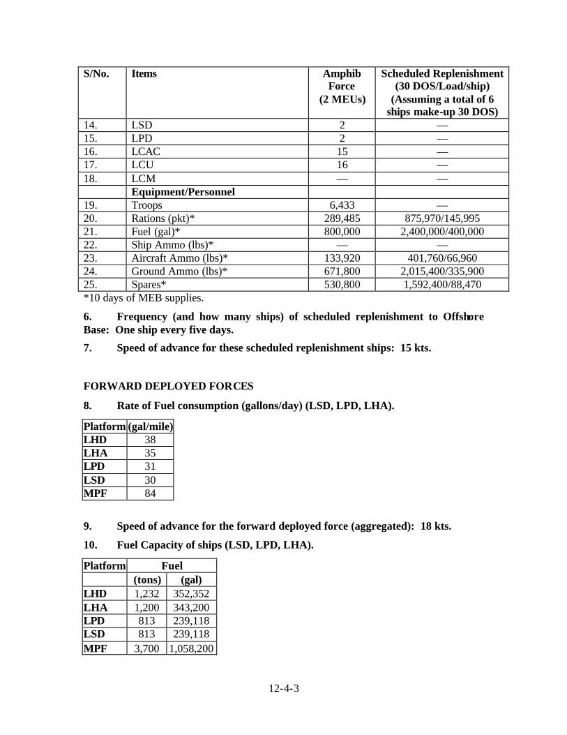
12-4-3
S/No. Items Amphib Force
(2 MEUs)
Scheduled Replenishment (30 DOS/Load/ship)
(Assuming a total of 6 ships make-up 30 DOS)
14. LSD 2 — 15. LPD 2 — 16. LCAC 15 — 17. LCU 16 — 18. LCM — — Equipment/Personnel 19. Troops 6,433 — 20. Rations (pkt)* 289,485 875,970/145,995 21. Fuel (gal)* 800,000 2,400,000/400,000 22. Ship Ammo (lbs)* — — 23. Aircraft Ammo (lbs)* 133,920 401,760/66,960 24. Ground Ammo (lbs)* 671,800 2,015,400/335,900 25. Spares* 530,800 1,592,400/88,470 *10 days of MEB supplies.
6. Frequency (and how many ships) of scheduled replenishment to Offshore Base: One ship every five days.
7. Speed of advance for these scheduled replenishment ships: 15 kts.
FORWARD DEPLOYED FORCES
8. Rate of Fuel consumption (gallons/day) (LSD, LPD, LHA).
Platform (gal/mile) LHD 38 LHA 35 LPD 31 LSD 30 MPF 84
9. Speed of advance for the forward deployed force (aggregated): 18 kts.
10. Fuel Capacity of ships (LSD, LPD, LHA).
Platform Fuel (tons) (gal) LHD 1,232 352,352 LHA 1,200 343,200 LPD 813 239,118 LSD 813 239,118 MPF 3,700 1,058,200
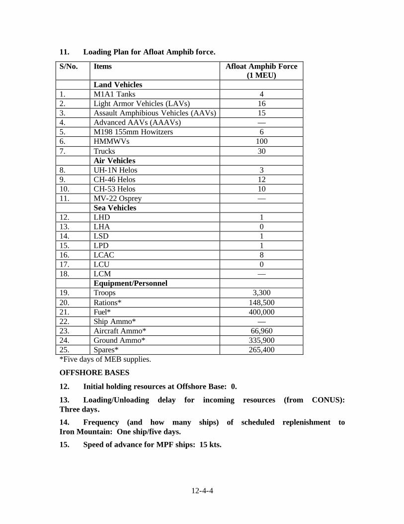
12-4-4
11. Loading Plan for Afloat Amphib force.
S/No. Items Afloat Amphib Force (1 MEU)
Land Vehicles 1. M1A1 Tanks 4 2. Light Armor Vehicles (LAVs) 16 3. Assault Amphibious Vehicles (AAVs) 15 4. Advanced AAVs (AAAVs) — 5. M198 155mm Howitzers 6 6. HMMWVs 100 7. Trucks 30 Air Vehicles 8. UH-1N Helos 3 9. CH-46 Helos 12 10. CH-53 Helos 10 11. MV-22 Osprey — Sea Vehicles 12. LHD 1 13. LHA 0 14. LSD 1 15. LPD 1 16. LCAC 8 17. LCU 0 18. LCM — Equipment/Personnel 19. Troops 3,300 20. Rations* 148,500 21. Fuel* 400,000 22. Ship Ammo* — 23. Aircraft Ammo* 66,960 24. Ground Ammo* 335,900 25. Spares* 265,400 *Five days of MEB supplies.
OFFSHORE BASES
12. Initial holding resources at Offshore Base: 0.
13. Loading/Unloading delay for incoming resources (from CONUS): Three days.
14. Frequency (and how many ships) of scheduled replenishment to Iron Mountain: One ship/five days.
15. Speed of advance for MPF ships: 15 kts.
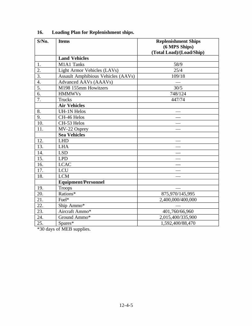
12-4-5
16. Loading Plan for Replenishment ships.
S/No. Items Replenishment Ships (6 MPS Ships)
(Total Load)/(Load/Ship) Land Vehicles 1. M1A1 Tanks 58/9 2. Light Armor Vehicles (LAVs) 25/4 3. Assault Amphibious Vehicles (AAVs) 109/18 4. Advanced AAVs (AAAVs) — 5. M198 155mm Howitzers 30/5 6. HMMWVs 748/124 7. Trucks 447/74 Air Vehicles 8. UH-1N Helos — 9. CH-46 Helos — 10. CH-53 Helos — 11. MV-22 Osprey — Sea Vehicles 12. LHD — 13. LHA — 14. LSD — 15. LPD — 16. LCAC — 17. LCU — 18. LCM — Equipment/Personnel 19. Troops — 20. Rations* 875,970/145,995 21. Fuel* 2,400,000/400,000 22. Ship Ammo* — 23. Aircraft Ammo* 401,760/66,960 24. Ground Ammo* 2,015,400/335,900 25. Spares* 1,592,400/88,470 *30 days of MEB supplies.
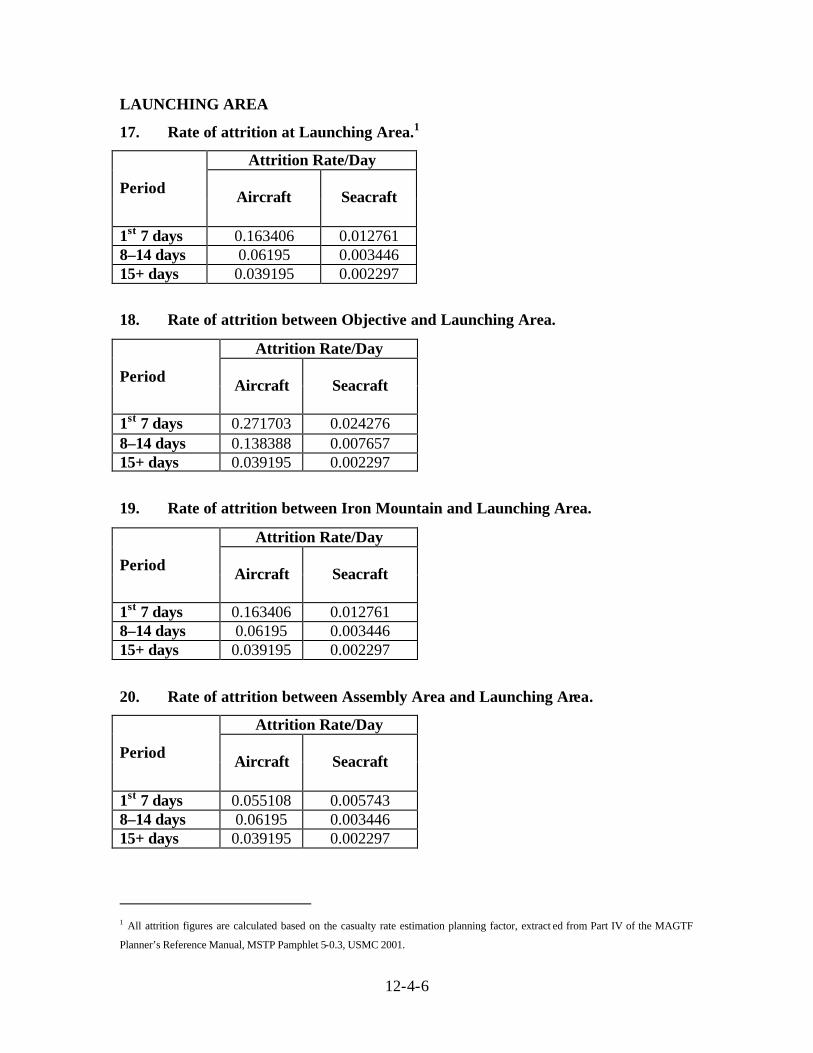
12-4-6
LAUNCHING AREA
17. Rate of attrition at Launching Area.1
Attrition Rate/Day
Period Aircraft Seacraft
1st 7 days 0.163406 0.012761 8–14 days 0.06195 0.003446 15+ days 0.039195 0.002297
18. Rate of attrition between Objective and Launching Area.
Attrition Rate/Day
Period Aircraft Seacraft
1st 7 days 0.271703 0.024276 8–14 days 0.138388 0.007657 15+ days 0.039195 0.002297
19. Rate of attrition between Iron Mountain and Launching Area.
Attrition Rate/Day
Period Aircraft Seacraft
1st 7 days 0.163406 0.012761 8–14 days 0.06195 0.003446 15+ days 0.039195 0.002297
20. Rate of attrition between Assembly Area and Launching Area.
Attrition Rate/Day
Period Aircraft Seacraft
1st 7 days 0.055108 0.005743 8–14 days 0.06195 0.003446 15+ days 0.039195 0.002297
1 All attrition figures are calculated based on the casualty rate estimation planning factor, extract ed from Part IV of the MAGTF
Planner’s Reference Manual, MSTP Pamphlet 5-0.3, USMC 2001.
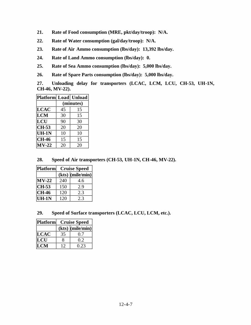
12-4-7
21. Rate of Food consumption (MRE, pkt/day/troop): N/A.
22. Rate of Water consumption (gal/day/troop): N/A.
23. Rate of Air Ammo consumption (lbs/day): 13,392 lbs/day.
24. Rate of Land Ammo consumption (lbs/day): 0.
25. Rate of Sea Ammo consumption (lbs/day): 5,000 lbs/day.
26. Rate of Spare Parts consumption (lbs/day): 5,000 lbs/day.
27. Unloading delay for transporters (LCAC, LCM, LCU, CH-53, UH-1N, CH-46, MV-22).
Platform Load Unload (minutes) LCAC 45 15 LCM 30 15 LCU 90 30 CH-53 20 20 UH-1N 10 10 CH-46 15 15 MV-22 20 20
28. Speed of Air transporters (CH-53, UH-1N, CH-46, MV-22).
Platform Cruise Speed (kts) (mile/min) MV-22 240 4.6 CH-53 150 2.9 CH-46 120 2.3 UH-1N 120 2.3
29. Speed of Surface transporters (LCAC, LCU, LCM, etc.).
Platform Cruise Speed (kts) (mile/min) LCAC 35 0.7 LCU 8 0.2 LCM 12 0.23
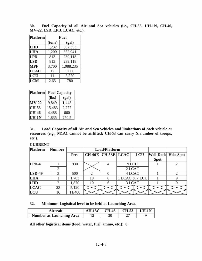
12-4-8
30. Fuel Capacity of all Air and Sea vehicles (i.e., CH-53, UH-1N, CH-46, MV-22, LSD, LPD, LCAC, etc.).
Platform Fuel (tons) (gal) LHD 1,232 362,353 LHA 1,200 352,941 LPD 813 239,118 LSD 813 239,118 MPF 3,700 1,088,235 LCAC 17 5,000 LCU 11 3,220 LCM 2.65 780
Platform Fuel Capacity (lbs) (gal) MV-22 9,849 1,448 CH-53 15,483 2,277 CH-46 4,488 660 UH-1N 1,835 270.5
31. Load Capacity of all Air and Sea vehicles and limitations of each vehicle or resources (e.g., M1A1 cannot be airlifted; CH-53 can carry X number of troops, etc.).
CURRENT Load/Platform Platform Number
Pers CH-46E CH-53E LCAC LCU Well-Deck Spot
Helo Spot
1 9 LCU LPD-4 2
930 4 2 LCAC
1 2
LSD-49 3 500 2 0 4 LCAC 1 2 LHA 1 1,703 10 6 1 LCAC & 7 LCU 1 9 LHD 2 1,870 10 6 3 LCAC 1 9 LCAC 23 5/120 LCU 16 11/400
32. Minimum Logistical level to be held at Launching Area.
Aircraft AH-1W CH-46 CH-53 UH-1N Number at Launching Area 12 30 27 9
All other logistical items (food, water, fuel, ammo, etc.): 0.
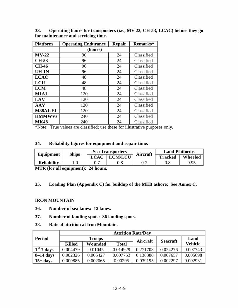
12-4-9
33. Operating hours for transporters (i.e., MV-22, CH-53, LCAC) before they go for maintenance and servicing time.
Platform Operating Endurance Repair Remarks* (hours) MV-22 96 24 Classified CH-53 96 24 Classified CH-46 96 24 Classified UH-1N 96 24 Classified LCAC 48 24 Classified LCU 48 24 Classified LCM 48 24 Classified M1A1 120 24 Classified LAV 120 24 Classified AAV 120 24 Classified M88A1-E1 120 24 Classified HMMWVs 240 24 Classified MK48 240 24 Classified *Note: True values are classified; use these for illustrative purposes only.
34. Reliability figures for equipment and repair time.
Sea Transporters Land Platforms Equipment Ships LCAC LCM/LCU
Aircraft Tracked Wheeled
Reliability 1.0 0.7 0.8 0.7 0.8 0.95 MTR (for all equipment): 24 hours.
35. Loading Plan (Appendix C) for buildup of the MEB ashore: See Annex C.
IRON MOUNTAIN
36. Number of sea lanes: 12 lanes.
37. Number of landing spots: 36 landing spots.
38. Rate of attrition at Iron Mountain.
Attrition Rate/Day Troops Period
Killed Wounded Total Aircraft Seacraft Land
Vehicle 1st 7 days 0.004479 0.01045 0.014929 0.271703 0.024276 0.007743 8–14 days 0.002326 0.005427 0.007753 0.138388 0.007657 0.005698 15+ days 0.000885 0.002065 0.00295 0.039195 0.002297 0.002931
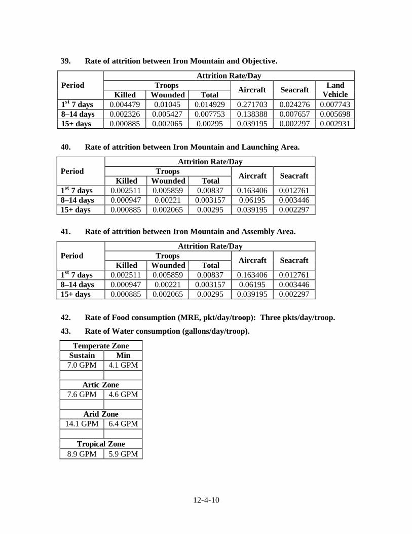
12-4-10
39. Rate of attrition between Iron Mountain and Objective.
Attrition Rate/Day Troops Period
Killed Wounded Total Aircraft Seacraft Land
Vehicle 1st 7 days 0.004479 0.01045 0.014929 0.271703 0.024276 0.007743 8–14 days 0.002326 0.005427 0.007753 0.138388 0.007657 0.005698 15+ days 0.000885 0.002065 0.00295 0.039195 0.002297 0.002931
40. Rate of attrition between Iron Mountain and Launching Area.
Attrition Rate/Day Troops Period
Killed Wounded Total Aircraft Seacraft
1st 7 days 0.002511 0.005859 0.00837 0.163406 0.012761 8–14 days 0.000947 0.00221 0.003157 0.06195 0.003446 15+ days 0.000885 0.002065 0.00295 0.039195 0.002297
41. Rate of attrition between Iron Mountain and Assembly Area.
Attrition Rate/Day Troops Period
Killed Wounded Total Aircraft Seacraft
1st 7 days 0.002511 0.005859 0.00837 0.163406 0.012761 8–14 days 0.000947 0.00221 0.003157 0.06195 0.003446 15+ days 0.000885 0.002065 0.00295 0.039195 0.002297
42. Rate of Food consumption (MRE, pkt/day/troop): Three pkts/day/troop.
43. Rate of Water consumption (gallons/day/troop).
Temperate Zone Sustain Min 7.0 GPM 4.1 GPM
Artic Zone
7.6 GPM 4.6 GPM Arid Zone
14.1 GPM 6.4 GPM
Tropical Zone 8.9 GPM 5.9 GPM
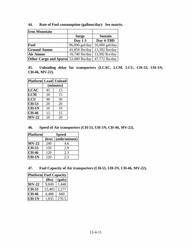
12-4-11
44. Rate of Fuel consumption (gallons/day): See matrix.
Iron Mountain Surge Sustain Day 1-3 Day 4-TBD Fuel 96,000 gal/day 16,000 gal/day Ground Ammo 41,850 lbs/day 13,392 lbs/day Air Ammo 16,740 lbs/day 13,392 lbs/day Other Cargo and Spares 53,080 lbs/day 47,772 lbs/day 45. Unloading delay for transporters (LCAC, LCM, LCU, CH-53, UH-1N, CH-46, MV-22). Platform Load Unload (minutes) LCAC 45 15 LCM 30 15 LCU 90 30 CH-53 20 20 UH-1N 10 10 CH-46 15 15 MV-22 20 20
46. Speed of Air transporters (CH-53, UH-1N, CH-46, MV-22).
Platform Speed (kts) (mile/minute) MV-22 240 4.6 CH-53 150 2.9 CH-46 120 2.3 UH-1N 120 2.3
47. Fuel Capacity of Air transporters (CH-53, UH-1N, CH-46, MV-22).
Platform Fuel Capacity (lbs) (gals) MV-22 9,849 1,448 CH-53 15,483 2,277 CH-46 4,488 660 UH-1N 1,835 270.5
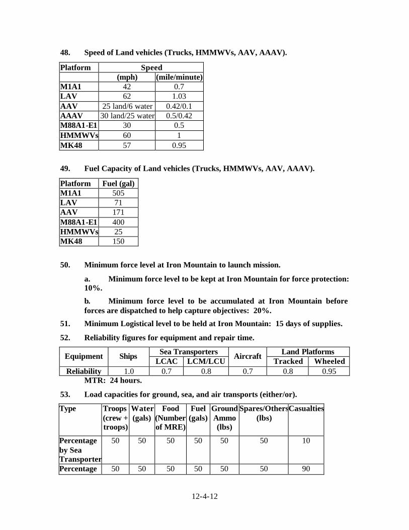
12-4-12
48. Speed of Land vehicles (Trucks, HMMWVs, AAV, AAAV).
Platform Speed (mph) (mile/minute) M1A1 42 0.7 LAV 62 1.03 AAV 25 land/6 water 0.42/0.1 AAAV 30 land/25 water 0.5/0.42 M88A1-E1 30 0.5 HMMWVs 60 1 MK48 57 0.95
49. Fuel Capacity of Land vehicles (Trucks, HMMWVs, AAV, AAAV).
Platform Fuel (gal) M1A1 505 LAV 71 AAV 171 M88A1-E1 400 HMMWVs 25 MK48 150
50. Minimum force level at Iron Mountain to launch mission.
a. Minimum force level to be kept at Iron Mountain for force protection: 10%.
b. Minimum force level to be accumulated at Iron Mountain before forces are dispatched to help capture objectives: 20%.
51. Minimum Logistical level to be held at Iron Mountain: 15 days of supplies.
52. Reliability figures for equipment and repair time.
Sea Transporters Land Platforms Equipment Ships LCAC LCM/LCU
Aircraft Tracked Wheeled
Reliability 1.0 0.7 0.8 0.7 0.8 0.95 MTR: 24 hours.
53. Load capacities for ground, sea, and air transports (either/or).
Type Troops (crew + troops)
Water (gals)
Food (Number of MRE)
Fuel (gals)
Ground Ammo (lbs)
Spares/Others (lbs)
Casualties
Percentage by Sea Transporter
50 50 50 50 50 50 10
Percentage 50 50 50 50 50 50 90
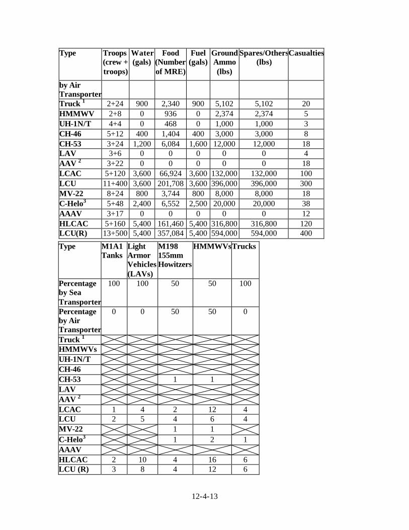
12-4-13
Type Troops (crew + troops)
Water (gals)
Food (Number of MRE)
Fuel (gals)
Ground Ammo (lbs)
Spares/Others (lbs)
Casualties
by Air Transporter Truck 1 2+24 900 2,340 900 5,102 5,102 20 HMMWV 2+8 0 936 0 2,374 2,374 5 UH-1N/T 4+4 0 468 0 1,000 1,000 3 CH-46 5+12 400 1,404 400 3,000 3,000 8 CH-53 3+24 1,200 6,084 1,600 12,000 12,000 18 LAV 3+6 0 0 0 0 0 4 AAV 2 3+22 0 0 0 0 0 18 LCAC 5+120 3,600 66,924 3,600 132,000 132,000 100 LCU 11+400 3,600 201,708 3,600 396,000 396,000 300 MV-22 8+24 800 3,744 800 8,000 8,000 18 C-Helo3 5+48 2,400 6,552 2,500 20,000 20,000 38 AAAV 3+17 0 0 0 0 0 12 HLCAC 5+160 5,400 161,460 5,400 316,800 316,800 120 LCU(R) 13+500 5,400 357,084 5,400 594,000 594,000 400
Type M1A1 Tanks
Light Armor Vehicles (LAVs)
M198 155mm Howitzers
HMMWVsTrucks
Percentage by Sea Transporter
100 100 50 50 100
Percentage by Air Transporter
0 0 50 50 0
Truck 1 HMMWVs UH-1N/T CH-46 CH-53 1 1 LAV AAV 2 LCAC 1 4 2 12 4 LCU 2 5 4 6 4 MV-22 1 1 C-Helo3 1 2 1 AAAV HLCAC 2 10 4 16 6 LCU (R) 3 8 4 12 6
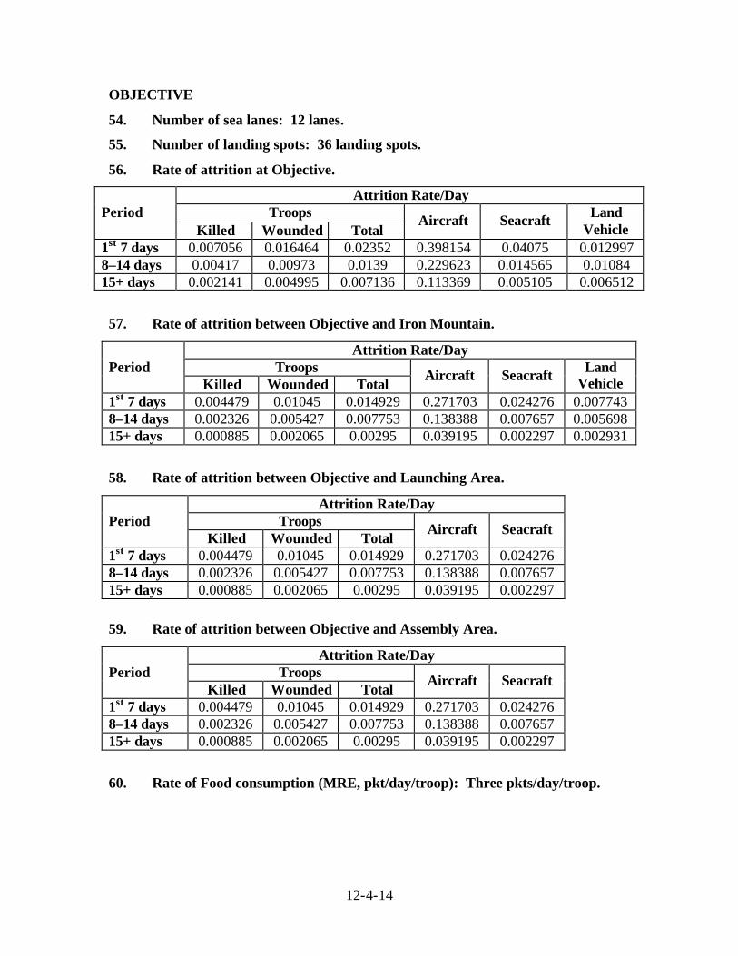
12-4-14
OBJECTIVE
54. Number of sea lanes: 12 lanes.
55. Number of landing spots: 36 landing spots.
56. Rate of attrition at Objective.
Attrition Rate/Day Troops Period
Killed Wounded Total Aircraft Seacraft Land
Vehicle 1st 7 days 0.007056 0.016464 0.02352 0.398154 0.04075 0.012997 8–14 days 0.00417 0.00973 0.0139 0.229623 0.014565 0.01084 15+ days 0.002141 0.004995 0.007136 0.113369 0.005105 0.006512
57. Rate of attrition between Objective and Iron Mountain.
Attrition Rate/Day Troops Period
Killed Wounded Total Aircraft Seacraft Land
Vehicle 1st 7 days 0.004479 0.01045 0.014929 0.271703 0.024276 0.007743 8–14 days 0.002326 0.005427 0.007753 0.138388 0.007657 0.005698 15+ days 0.000885 0.002065 0.00295 0.039195 0.002297 0.002931
58. Rate of attrition between Objective and Launching Area.
Attrition Rate/Day Troops Period
Killed Wounded Total Aircraft Seacraft
1st 7 days 0.004479 0.01045 0.014929 0.271703 0.024276 8–14 days 0.002326 0.005427 0.007753 0.138388 0.007657 15+ days 0.000885 0.002065 0.00295 0.039195 0.002297
59. Rate of attrition between Objective and Assembly Area.
Attrition Rate/Day Troops Period
Killed Wounded Total Aircraft Seacraft
1st 7 days 0.004479 0.01045 0.014929 0.271703 0.024276 8–14 days 0.002326 0.005427 0.007753 0.138388 0.007657 15+ days 0.000885 0.002065 0.00295 0.039195 0.002297
60. Rate of Food consumption (MRE, pkt/day/troop): Three pkts/day/troop.
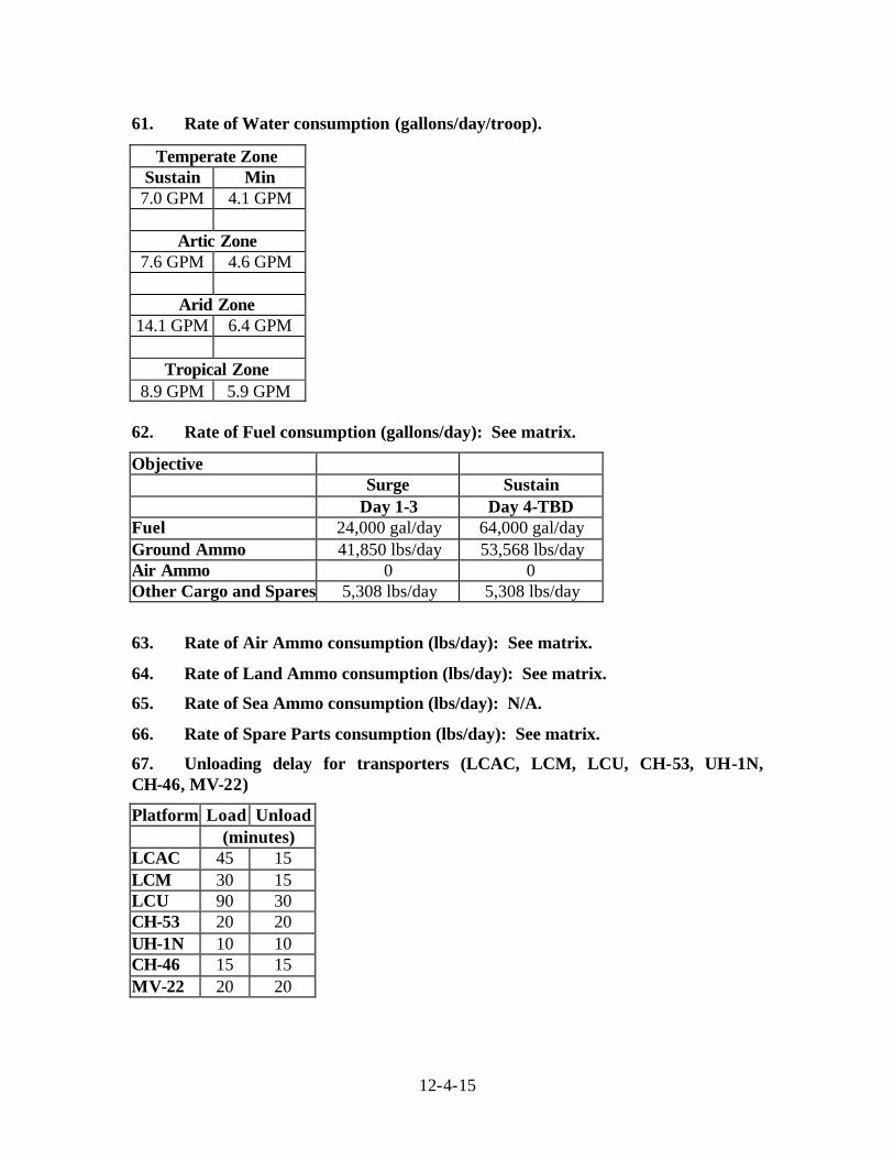
12-4-15
61. Rate of Water consumption (gallons/day/troop).
Temperate Zone Sustain Min 7.0 GPM 4.1 GPM
Artic Zone
7.6 GPM 4.6 GPM Arid Zone
14.1 GPM 6.4 GPM
Tropical Zone 8.9 GPM 5.9 GPM
62. Rate of Fuel consumption (gallons/day): See matrix.
Objective Surge Sustain Day 1-3 Day 4-TBD Fuel 24,000 gal/day 64,000 gal/day Ground Ammo 41,850 lbs/day 53,568 lbs/day Air Ammo 0 0 Other Cargo and Spares 5,308 lbs/day 5,308 lbs/day
63. Rate of Air Ammo consumption (lbs/day): See matrix.
64. Rate of Land Ammo consumption (lbs/day): See matrix.
65. Rate of Sea Ammo consumption (lbs/day): N/A.
66. Rate of Spare Parts consumption (lbs/day): See matrix.
67. Unloading delay for transporters (LCAC, LCM, LCU, CH-53, UH-1N, CH-46, MV-22)
Platform Load Unload (minutes)
LCAC 45 15 LCM 30 15 LCU 90 30 CH-53 20 20 UH-1N 10 10 CH-46 15 15 MV-22 20 20
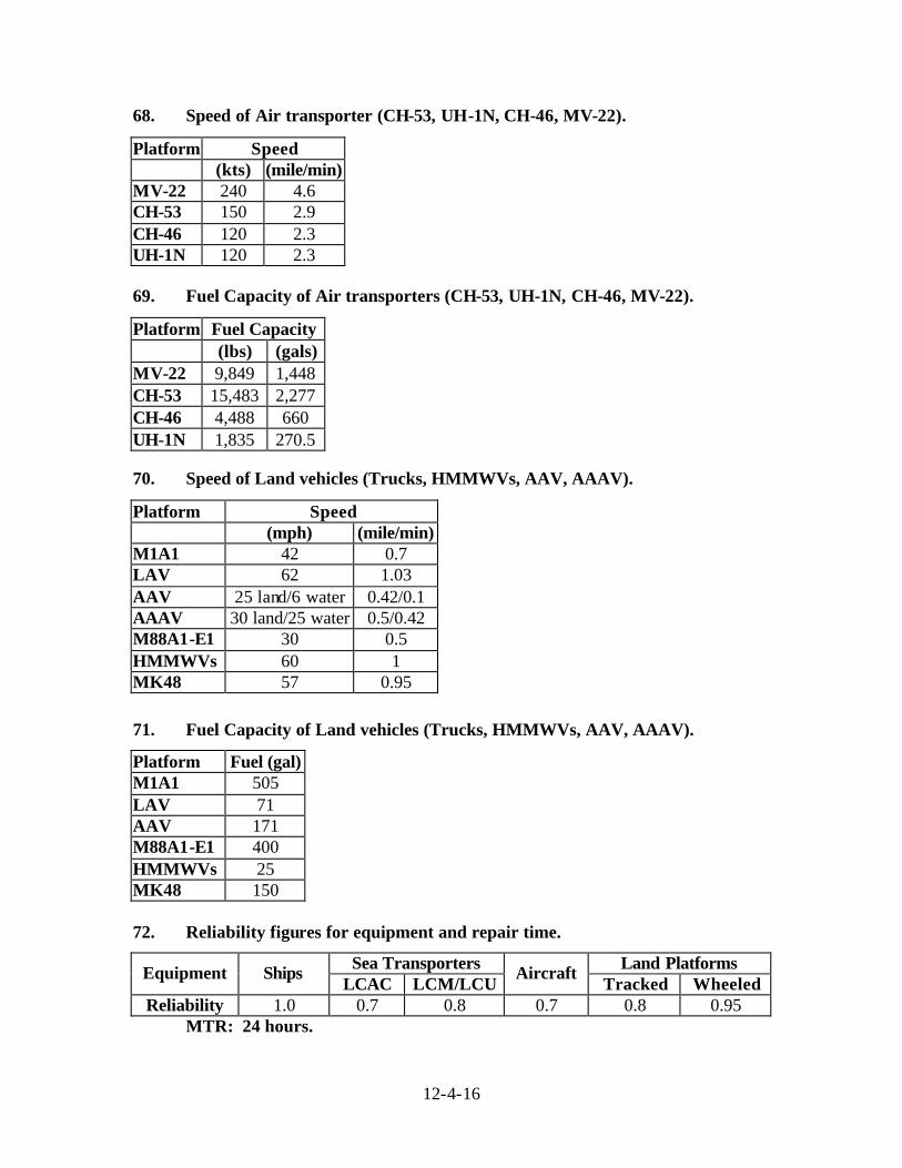
12-4-16
68. Speed of Air transporter (CH-53, UH-1N, CH-46, MV-22).
Platform Speed (kts) (mile/min) MV-22 240 4.6 CH-53 150 2.9 CH-46 120 2.3 UH-1N 120 2.3 69. Fuel Capacity of Air transporters (CH-53, UH-1N, CH-46, MV-22).
Platform Fuel Capacity (lbs) (gals) MV-22 9,849 1,448 CH-53 15,483 2,277 CH-46 4,488 660 UH-1N 1,835 270.5
70. Speed of Land vehicles (Trucks, HMMWVs, AAV, AAAV).
Platform Speed (mph) (mile/min) M1A1 42 0.7 LAV 62 1.03 AAV 25 land/6 water 0.42/0.1 AAAV 30 land/25 water 0.5/0.42 M88A1-E1 30 0.5 HMMWVs 60 1 MK48 57 0.95
71. Fuel Capacity of Land vehicles (Trucks, HMMWVs, AAV, AAAV).
Platform Fuel (gal) M1A1 505 LAV 71 AAV 171 M88A1-E1 400 HMMWVs 25 MK48 150 72. Reliability figures for equipment and repair time.
Sea Transporters Land Platforms Equipment Ships LCAC LCM/LCU
Aircraft Tracked Wheeled
Reliability 1.0 0.7 0.8 0.7 0.8 0.95 MTR: 24 hours.
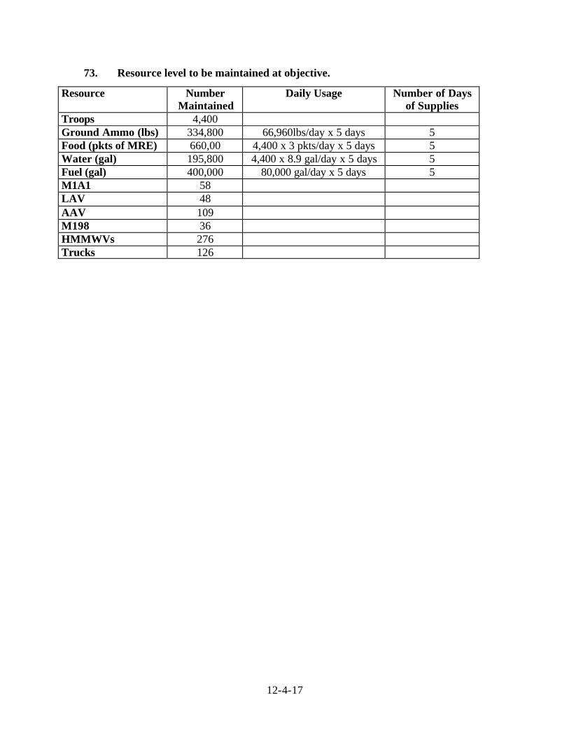
12-4-17
73. Resource level to be maintained at objective.
Resource Number Maintained
Daily Usage Number of Days of Supplies
Troops 4,400 Ground Ammo (lbs) 334,800 66,960lbs/day x 5 days 5 Food (pkts of MRE) 660,00 4,400 x 3 pkts/day x 5 days 5 Water (gal) 195,800 4,400 x 8.9 gal/day x 5 days 5 Fuel (gal) 400,000 80,000 gal/day x 5 days 5 M1A1 58 LAV 48 AAV 109 M198 36 HMMWVs 276 Trucks 126
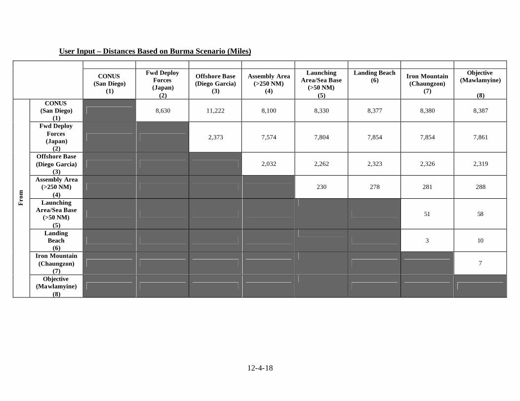
12-4-18
User Input – Distances Based on Burma Scenario (Miles)
CONUS (San Diego)
(1)
Fwd Deploy Forces (Japan)
(2)
Offshore Base (Diego Garcia)
(3)
Assembly Area (>250 NM)
(4)
Launching Area/Sea Base
(>50 NM) (5)
Landing Beach (6)
Iron Mountain (Chaungzon)
(7)
Objective (Mawlamyine)
(8)
CONUS (San Diego)
(1) 8,630 11,222 8,100 8,330 8,377 8,380 8,387
Fwd Deploy Forces (Japan)
(2)
2,373 7,574 7,804 7,854 7,854 7,861
Offshore Base (Diego Garcia)
(3) 2,032 2,262 2,323 2,326 2,319
Assembly Area (>250 NM)
(4) 230 278 281 288
Launching Area/Sea Base
(>50 NM) (5)
51 58
Landing Beach
(6)
3 10
Iron Mountain (Chaungzon)
(7)
7
Fro
m
Objective (Mawlamyine)
(8)
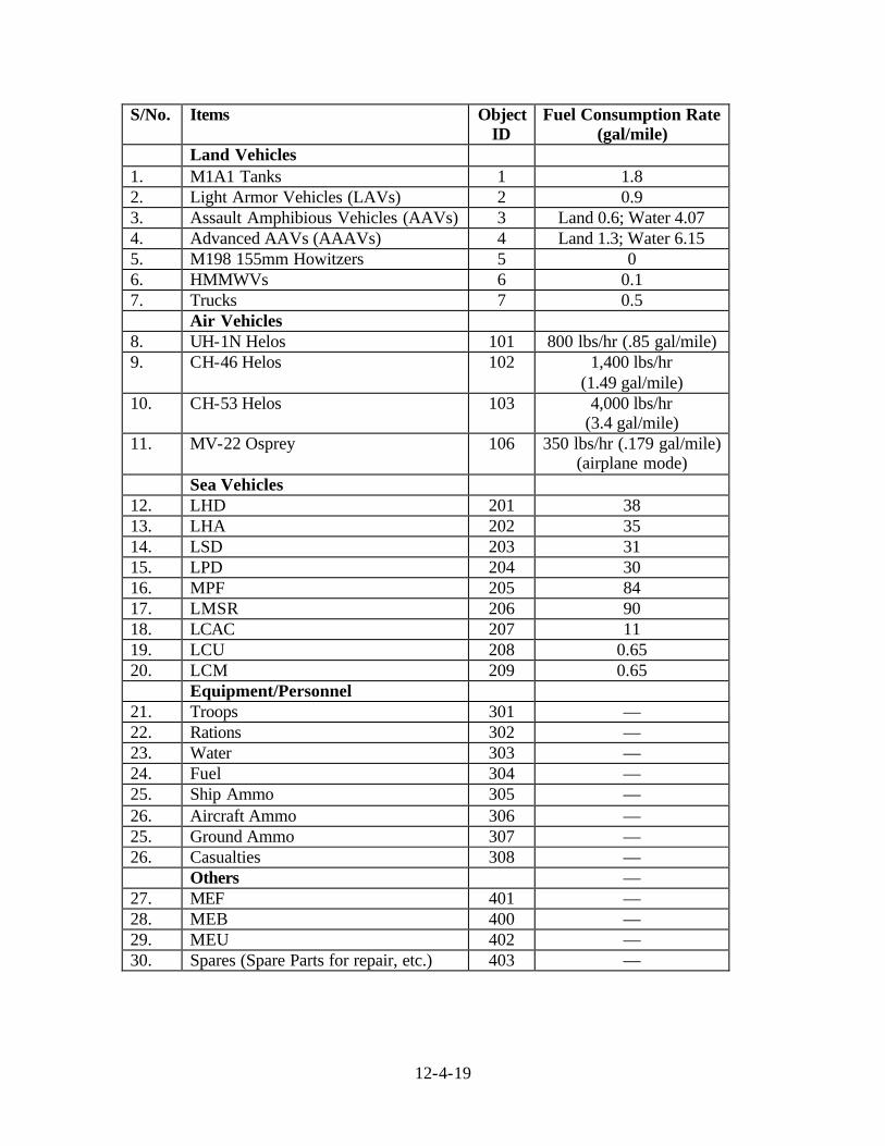
12-4-19
S/No. Items Object ID
Fuel Consumption Rate (gal/mile)
Land Vehicles 1. M1A1 Tanks 1 1.8 2. Light Armor Vehicles (LAVs) 2 0.9 3. Assault Amphibious Vehicles (AAVs) 3 Land 0.6; Water 4.07 4. Advanced AAVs (AAAVs) 4 Land 1.3; Water 6.15 5. M198 155mm Howitzers 5 0 6. HMMWVs 6 0.1 7. Trucks 7 0.5 Air Vehicles 8. UH-1N Helos 101 800 lbs/hr (.85 gal/mile) 9. CH-46 Helos 102 1,400 lbs/hr
(1.49 gal/mile) 10. CH-53 Helos 103 4,000 lbs/hr
(3.4 gal/mile) 11. MV-22 Osprey 106 350 lbs/hr (.179 gal/mile)
(airplane mode) Sea Vehicles 12. LHD 201 38 13. LHA 202 35 14. LSD 203 31 15. LPD 204 30 16. MPF 205 84 17. LMSR 206 90 18. LCAC 207 11 19. LCU 208 0.65 20. LCM 209 0.65 Equipment/Personnel 21. Troops 301 — 22. Rations 302 — 23. Water 303 — 24. Fuel 304 — 25. Ship Ammo 305 — 26. Aircraft Ammo 306 — 25. Ground Ammo 307 — 26. Casualties 308 — Others — 27. MEF 401 — 28. MEB 400 — 29. MEU 402 — 30. Spares (Spare Parts for repair, etc.) 403 —
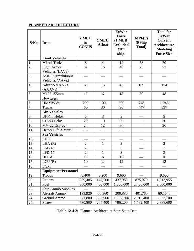
12-4-20
PLANNED ARCHITECTURE
S/No. Items 2 MEU
in CONUS
1 MEU Afloat
ExWar Force
(1 MEB) Exclude 6
MPS ships
MPF(F) (6 Ship Total)
Total for ExWar Current
Architecture Modeling Force Size
Land Vehicles 1. M1A1 Tanks 8 4 12 58 70 2. Light Armor
Vehicles (LAVs) 32 16 48 25 73
3. Assault Amphibious Vehicles (AAVs)
— — — — —
4. Advanced AAVs (AAAVs)
30 15 45 109 154
5. M198 155mm Howitzers
12 6 18 30 48
6. HMMWVs 200 100 300 748 1,048 7. Trucks 60 30 90 447 537 Air Vehicles 8. UH-1T Helos 6 3 9 — 9 9. CH-53 Helos 20 10 30 — 30 10. MV-22 Osprey 24 12 36 — 36 11. Heavy Lift Aircraft — — — — — Sea Vehicles 12. LHD — — — — — 13. LHA (R) 2 1 3 — 3 14. LSD-49 2 1 3 — 3 15. LPD-17 2 1 3 — 3 16. HLCAC 10 6 16 — 16 17. LCU (R) 10 2 12 — 12 18. LCM — — — — — Equipment/Personnel 19. Troops 6,400 3,200 9,600 — 9,600 20. Rations 289,485 148,500 437,985 875,970 1,313,955 21. Fuel 800,000 400,000 1,200,000 2,400,000 3,600,000 22. Ship Ammo Supplies — — — — — 23. Aircraft Ammo 133,920 66,960 200,880 401,760 602,640 24. Ground Ammo 671,800 335,900 1,007,700 2,015,400 3,023,100 25. Spares 530,800 265,400 796,200 1,592,400 2,388,600
Table 12-4-2: Planned Architecture Start State Data
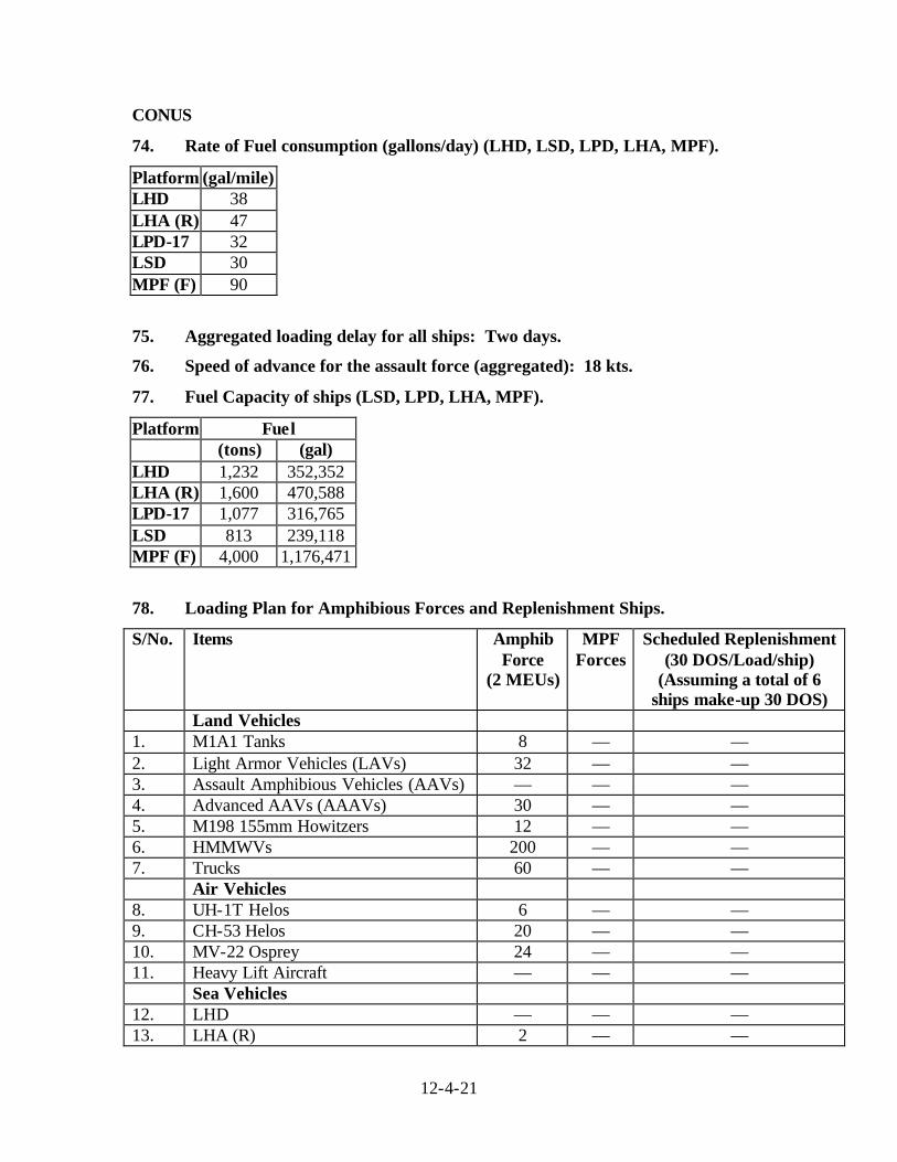
12-4-21
CONUS
74. Rate of Fuel consumption (gallons/day) (LHD, LSD, LPD, LHA, MPF).
Platform (gal/mile) LHD 38 LHA (R) 47 LPD-17 32 LSD 30 MPF (F) 90
75. Aggregated loading delay for all ships: Two days.
76. Speed of advance for the assault force (aggregated): 18 kts.
77. Fuel Capacity of ships (LSD, LPD, LHA, MPF).
Platform Fuel (tons) (gal) LHD 1,232 352,352 LHA (R) 1,600 470,588 LPD-17 1,077 316,765 LSD 813 239,118 MPF (F) 4,000 1,176,471
78. Loading Plan for Amphibious Forces and Replenishment Ships.
S/No. Items Amphib Force
(2 MEUs)
MPF Forces
Scheduled Replenishment (30 DOS/Load/ship)
(Assuming a total of 6 ships make-up 30 DOS)
Land Vehicles 1. M1A1 Tanks 8 — — 2. Light Armor Vehicles (LAVs) 32 — — 3. Assault Amphibious Vehicles (AAVs) — — — 4. Advanced AAVs (AAAVs) 30 — — 5. M198 155mm Howitzers 12 — — 6. HMMWVs 200 — — 7. Trucks 60 — — Air Vehicles 8. UH-1T Helos 6 — — 9. CH-53 Helos 20 — — 10. MV-22 Osprey 24 — — 11. Heavy Lift Aircraft — — — Sea Vehicles 12. LHD — — — 13. LHA (R) 2 — —
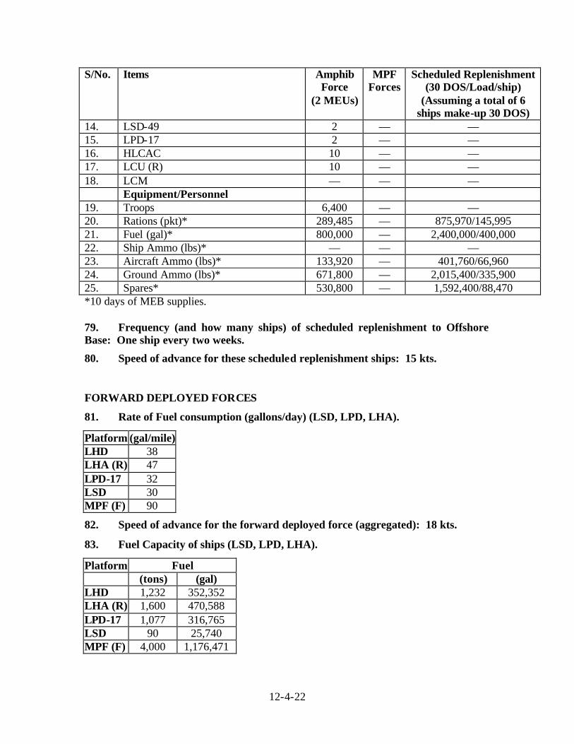
12-4-22
S/No. Items Amphib Force
(2 MEUs)
MPF Forces
Scheduled Replenishment (30 DOS/Load/ship)
(Assuming a total of 6 ships make-up 30 DOS)
14. LSD-49 2 — — 15. LPD-17 2 — — 16. HLCAC 10 — — 17. LCU (R) 10 — — 18. LCM — — — Equipment/Personnel 19. Troops 6,400 — — 20. Rations (pkt)* 289,485 — 875,970/145,995 21. Fuel (gal)* 800,000 — 2,400,000/400,000 22. Ship Ammo (lbs)* — — — 23. Aircraft Ammo (lbs)* 133,920 — 401,760/66,960 24. Ground Ammo (lbs)* 671,800 — 2,015,400/335,900 25. Spares* 530,800 — 1,592,400/88,470 *10 days of MEB supplies. 79. Frequency (and how many ships) of scheduled replenishment to Offshore Base: One ship every two weeks.
80. Speed of advance for these scheduled replenishment ships: 15 kts.
FORWARD DEPLOYED FORCES
81. Rate of Fuel consumption (gallons/day) (LSD, LPD, LHA).
Platform (gal/mile) LHD 38 LHA (R) 47 LPD-17 32 LSD 30 MPF (F) 90
82. Speed of advance for the forward deployed force (aggregated): 18 kts.
83. Fuel Capacity of ships (LSD, LPD, LHA).
Platform Fuel (tons) (gal) LHD 1,232 352,352 LHA (R) 1,600 470,588 LPD-17 1,077 316,765 LSD 90 25,740 MPF (F) 4,000 1,176,471
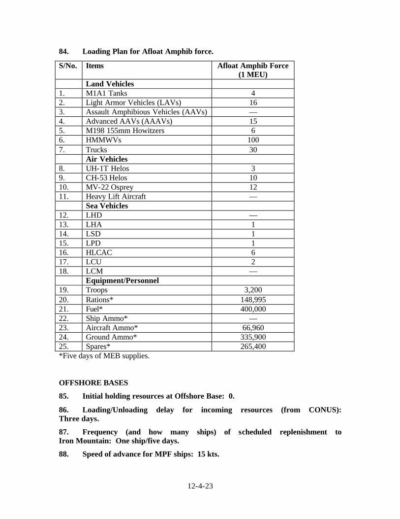
12-4-23
84. Loading Plan for Afloat Amphib force.
S/No. Items Afloat Amphib Force (1 MEU)
Land Vehicles 1. M1A1 Tanks 4 2. Light Armor Vehicles (LAVs) 16 3. Assault Amphibious Vehicles (AAVs) — 4. Advanced AAVs (AAAVs) 15 5. M198 155mm Howitzers 6 6. HMMWVs 100 7. Trucks 30 Air Vehicles 8. UH-1T Helos 3 9. CH-53 Helos 10 10. MV-22 Osprey 12 11. Heavy Lift Aircraft — Sea Vehicles 12. LHD — 13. LHA 1 14. LSD 1 15. LPD 1 16. HLCAC 6 17. LCU 2 18. LCM — Equipment/Personnel 19. Troops 3,200 20. Rations* 148,995 21. Fuel* 400,000 22. Ship Ammo* — 23. Aircraft Ammo* 66,960 24. Ground Ammo* 335,900 25. Spares* 265,400 *Five days of MEB supplies.
OFFSHORE BASES
85. Initial holding resources at Offshore Base: 0.
86. Loading/Unloading delay for incoming resources (from CONUS): Three days.
87. Frequency (and how many ships) of scheduled replenishment to Iron Mountain: One ship/five days.
88. Speed of advance for MPF ships: 15 kts.
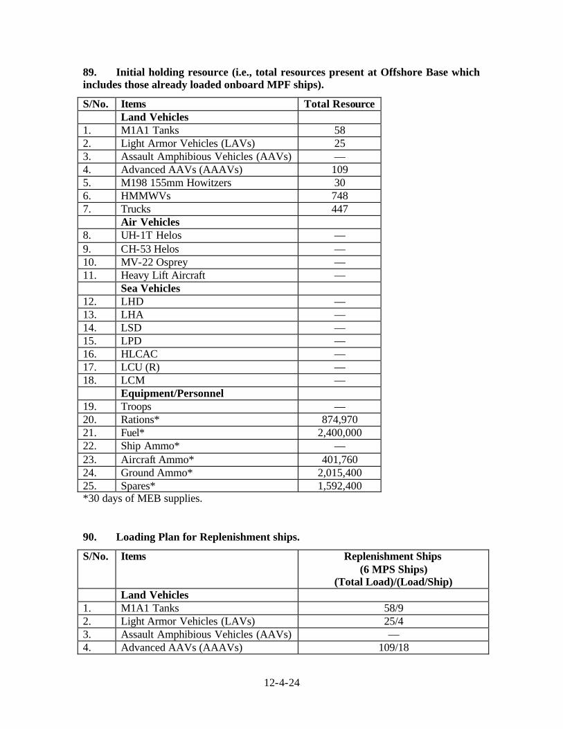
12-4-24
89. Initial holding resource (i.e., total resources present at Offshore Base which includes those already loaded onboard MPF ships).
S/No. Items Total Resource Land Vehicles 1. M1A1 Tanks 58 2. Light Armor Vehicles (LAVs) 25 3. Assault Amphibious Vehicles (AAVs) — 4. Advanced AAVs (AAAVs) 109 5. M198 155mm Howitzers 30 6. HMMWVs 748 7. Trucks 447 Air Vehicles 8. UH-1T Helos — 9. CH-53 Helos — 10. MV-22 Osprey — 11. Heavy Lift Aircraft — Sea Vehicles 12. LHD — 13. LHA — 14. LSD — 15. LPD — 16. HLCAC — 17. LCU (R) — 18. LCM — Equipment/Personnel 19. Troops — 20. Rations* 874,970 21. Fuel* 2,400,000 22. Ship Ammo* — 23. Aircraft Ammo* 401,760 24. Ground Ammo* 2,015,400 25. Spares* 1,592,400 *30 days of MEB supplies.
90. Loading Plan for Replenishment ships.
S/No. Items Replenishment Ships (6 MPS Ships)
(Total Load)/(Load/Ship) Land Vehicles 1. M1A1 Tanks 58/9 2. Light Armor Vehicles (LAVs) 25/4 3. Assault Amphibious Vehicles (AAVs) — 4. Advanced AAVs (AAAVs) 109/18
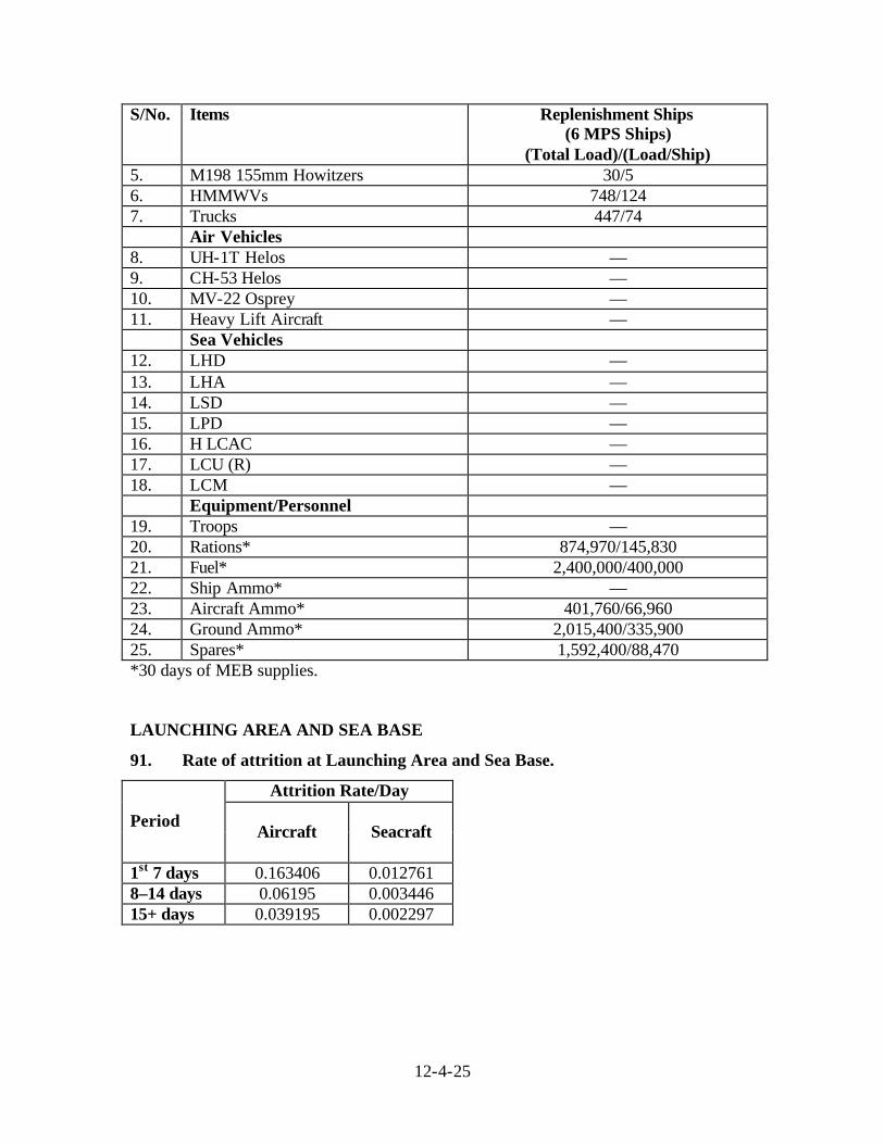
12-4-25
S/No. Items Replenishment Ships (6 MPS Ships)
(Total Load)/(Load/Ship) 5. M198 155mm Howitzers 30/5 6. HMMWVs 748/124 7. Trucks 447/74 Air Vehicles 8. UH-1T Helos — 9. CH-53 Helos — 10. MV-22 Osprey — 11. Heavy Lift Aircraft — Sea Vehicles 12. LHD — 13. LHA — 14. LSD — 15. LPD — 16. H LCAC — 17. LCU (R) — 18. LCM — Equipment/Personnel 19. Troops — 20. Rations* 874,970/145,830 21. Fuel* 2,400,000/400,000 22. Ship Ammo* — 23. Aircraft Ammo* 401,760/66,960 24. Ground Ammo* 2,015,400/335,900 25. Spares* 1,592,400/88,470 *30 days of MEB supplies.
LAUNCHING AREA AND SEA BASE
91. Rate of attrition at Launching Area and Sea Base.
Attrition Rate/Day
Period Aircraft Seacraft
1st 7 days 0.163406 0.012761 8–14 days 0.06195 0.003446 15+ days 0.039195 0.002297
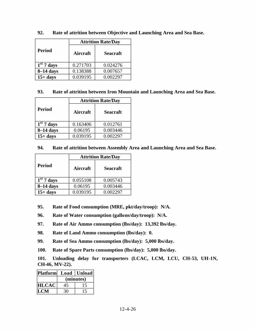
12-4-26
92. Rate of attrition between Objective and Launching Area and Sea Base.
Attrition Rate/Day
Period Aircraft Seacraft
1st 7 days 0.271703 0.024276 8–14 days 0.138388 0.007657 15+ days 0.039195 0.002297
93. Rate of attrition between Iron Mountain and Launching Area and Sea Base.
Attrition Rate/Day
Period Aircraft Seacraft
1st 7 days 0.163406 0.012761 8–14 days 0.06195 0.003446 15+ days 0.039195 0.002297 94. Rate of attrition between Assembly Area and Launching Area and Sea Base.
Attrition Rate/Day
Period Aircraft Seacraft
1st 7 days 0.055108 0.005743 8–14 days 0.06195 0.003446 15+ days 0.039195 0.002297
95. Rate of Food consumption (MRE, pkt/day/troop): N/A.
96. Rate of Water consumption (gallons/day/troop): N/A.
97. Rate of Air Ammo consumption (lbs/day): 13,392 lbs/day.
98. Rate of Land Ammo consumption (lbs/day): 0.
99. Rate of Sea Ammo consumption (lbs/day): 5,000 lbs/day.
100. Rate of Spare Parts consumption (lbs/day): 5,000 lbs/day.
101. Unloading delay for transporters (LCAC, LCM, LCU, CH-53, UH-1N, CH-46, MV-22).
Platform Load Unload (minutes) HLCAC 45 15 LCM 30 15
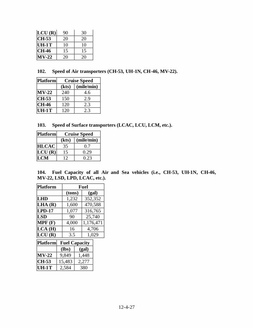
12-4-27
LCU (R) 90 30 CH-53 20 20 UH-1T 10 10 CH-46 15 15 MV-22 20 20
102. Speed of Air transporters (CH-53, UH-1N, CH-46, MV-22).
Platform Cruise Speed (kts) (mile/min) MV-22 240 4.6 CH-53 150 2.9 CH-46 120 2.3 UH-1T 120 2.3
103. Speed of Surface transporters (LCAC, LCU, LCM, etc.).
Platform Cruise Speed (kts) (mile/min) HLCAC 35 0.7 LCU (R) 15 0.29 LCM 12 0.23
104. Fuel Capacity of all Air and Sea vehicles (i.e., CH-53, UH-1N, CH-46, MV-22, LSD, LPD, LCAC, etc.).
Platform Fuel (tons) (gal) LHD 1,232 352,352 LHA (R) 1,600 470,588 LPD-17 1,077 316,765 LSD 90 25,740 MPF (F) 4,000 1,176,471 LCA (H) 16 4,706 LCU (R) 3.5 1,029
Platform Fuel Capacity (lbs) (gal) MV-22 9,849 1,448 CH-53 15,483 2,277 UH-1T 2,584 380
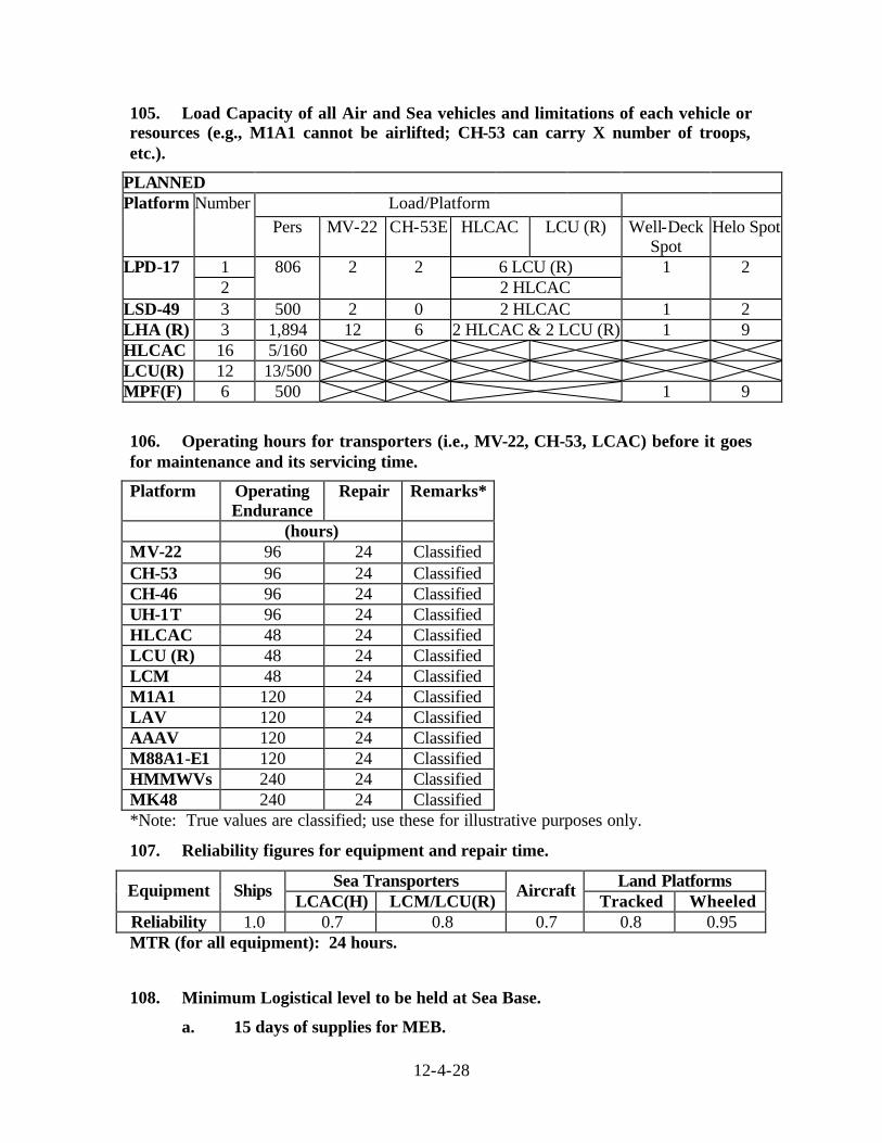
12-4-28
105. Load Capacity of all Air and Sea vehicles and limitations of each vehicle or resources (e.g., M1A1 cannot be airlifted; CH-53 can carry X number of troops, etc.).
PLANNED Load/Platform Platform Number
Pers MV-22 CH-53E HLCAC LCU (R) Well-Deck Spot
Helo Spot
1 6 LCU (R) LPD-17 2
806 2 2 2 HLCAC
1 2
LSD-49 3 500 2 0 2 HLCAC 1 2 LHA (R) 3 1,894 12 6 2 HLCAC & 2 LCU (R) 1 9 HLCAC 16 5/160 LCU(R) 12 13/500 MPF(F) 6 500 1 9
106. Operating hours for transporters (i.e., MV-22, CH-53, LCAC) before it goes for maintenance and its servicing time.
Platform Operating Endurance
Repair Remarks*
(hours) MV-22 96 24 Classified CH-53 96 24 Classified CH-46 96 24 Classified UH-1T 96 24 Classified HLCAC 48 24 Classified LCU (R) 48 24 Classified LCM 48 24 Classified M1A1 120 24 Classified LAV 120 24 Classified AAAV 120 24 Classified M88A1-E1 120 24 Classified HMMWVs 240 24 Classified MK48 240 24 Classified *Note: True values are classified; use these for illustrative purposes only.
107. Reliability figures for equipment and repair time.
Sea Transporters Land Platforms Equipment Ships LCAC(H) LCM/LCU(R)
Aircraft Tracked Wheeled
Reliability 1.0 0.7 0.8 0.7 0.8 0.95 MTR (for all equipment): 24 hours.
108. Minimum Logistical level to be held at Sea Base.
a. 15 days of supplies for MEB.
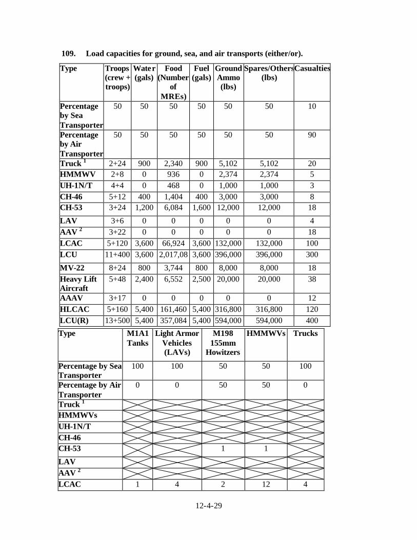
12-4-29
109. Load capacities for ground, sea, and air transports (either/or).
Type Troops (crew + troops)
Water (gals)
Food (Number
of MREs)
Fuel (gals)
Ground Ammo (lbs)
Spares/Others (lbs)
Casualties
Percentage by Sea Transporter
50 50 50 50 50 50 10
Percentage by Air Transporter
50 50 50 50 50 50 90
Truck 1 2+24 900 2,340 900 5,102 5,102 20 HMMWV 2+8 0 936 0 2,374 2,374 5 UH-1N/T 4+4 0 468 0 1,000 1,000 3 CH-46 5+12 400 1,404 400 3,000 3,000 8 CH-53 3+24 1,200 6,084 1,600 12,000 12,000 18
LAV 3+6 0 0 0 0 0 4 AAV 2 3+22 0 0 0 0 0 18 LCAC 5+120 3,600 66,924 3,600 132,000 132,000 100 LCU 11+400 3,600 2,017,08 3,600 396,000 396,000 300
MV-22 8+24 800 3,744 800 8,000 8,000 18 Heavy Lift Aircraft
5+48 2,400 6,552 2,500 20,000 20,000 38
AAAV 3+17 0 0 0 0 0 12 HLCAC 5+160 5,400 161,460 5,400 316,800 316,800 120 LCU(R) 13+500 5,400 357,084 5,400 594,000 594,000 400
Type M1A1 Tanks
Light Armor Vehicles (LAVs)
M198 155mm
Howitzers
HMMWVs Trucks
Percentage by Sea Transporter
100 100 50 50 100
Percentage by Air Transporter
0 0 50 50 0
Truck 1 HMMWVs UH-1N/T CH-46 CH-53 1 1
LAV AAV 2 LCAC 1 4 2 12 4
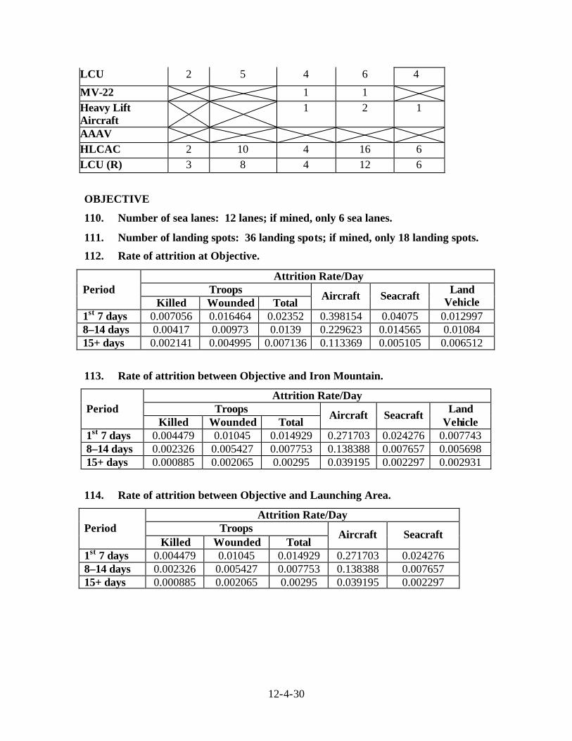
12-4-30
LCU 2 5 4 6 4
MV-22 1 1 Heavy Lift Aircraft
1 2 1
AAAV HLCAC 2 10 4 16 6 LCU (R) 3 8 4 12 6
OBJECTIVE
110. Number of sea lanes: 12 lanes; if mined, only 6 sea lanes.
111. Number of landing spots: 36 landing spots; if mined, only 18 landing spots.
112. Rate of attrition at Objective.
Attrition Rate/Day Troops Period
Killed Wounded Total Aircraft Seacraft Land
Vehicle 1st 7 days 0.007056 0.016464 0.02352 0.398154 0.04075 0.012997 8–14 days 0.00417 0.00973 0.0139 0.229623 0.014565 0.01084 15+ days 0.002141 0.004995 0.007136 0.113369 0.005105 0.006512
113. Rate of attrition between Objective and Iron Mountain.
Attrition Rate/Day Troops Period
Killed Wounded Total Aircraft Seacraft Land
Vehicle 1st 7 days 0.004479 0.01045 0.014929 0.271703 0.024276 0.007743 8–14 days 0.002326 0.005427 0.007753 0.138388 0.007657 0.005698 15+ days 0.000885 0.002065 0.00295 0.039195 0.002297 0.002931
114. Rate of attrition between Objective and Launching Area.
Attrition Rate/Day Troops Period
Killed Wounded Total Aircraft Seacraft
1st 7 days 0.004479 0.01045 0.014929 0.271703 0.024276 8–14 days 0.002326 0.005427 0.007753 0.138388 0.007657 15+ days 0.000885 0.002065 0.00295 0.039195 0.002297
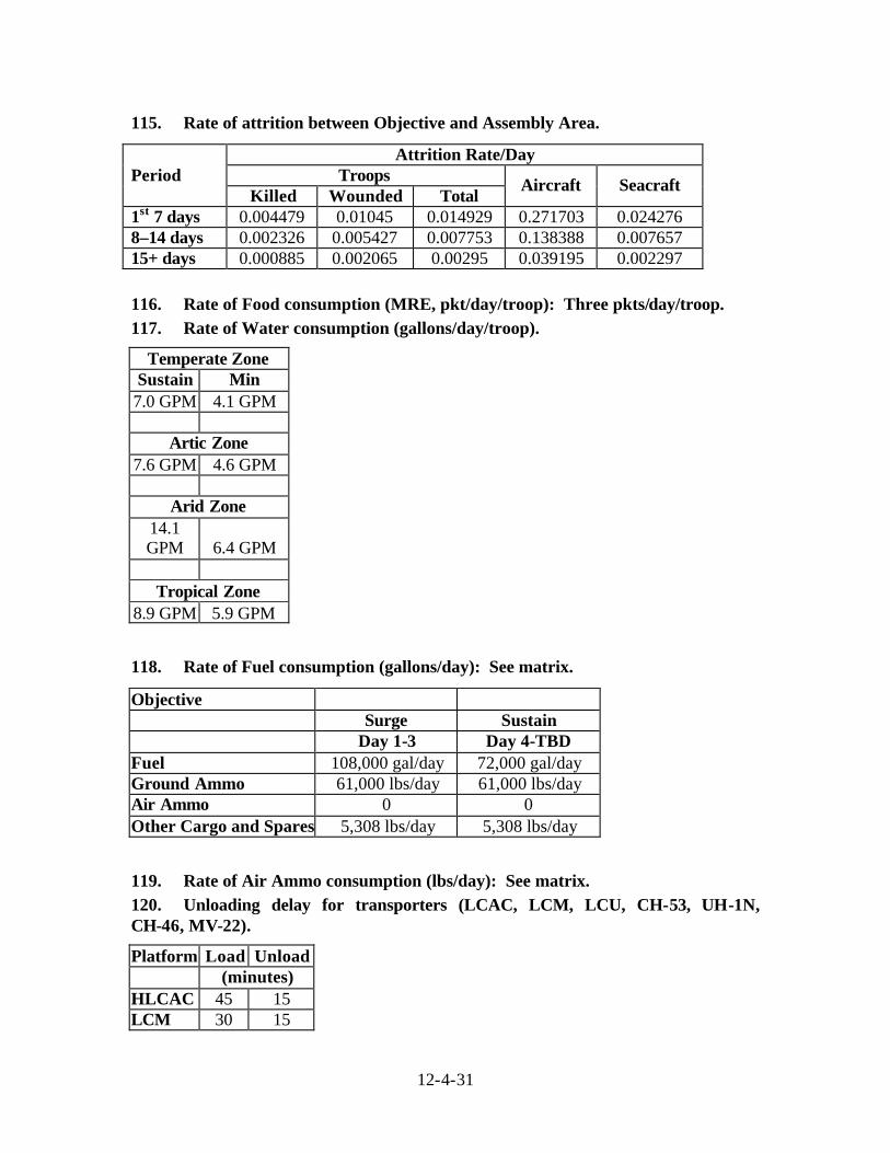
12-4-31
115. Rate of attrition between Objective and Assembly Area.
Attrition Rate/Day Troops Period
Killed Wounded Total Aircraft Seacraft
1st 7 days 0.004479 0.01045 0.014929 0.271703 0.024276 8–14 days 0.002326 0.005427 0.007753 0.138388 0.007657 15+ days 0.000885 0.002065 0.00295 0.039195 0.002297
116. Rate of Food consumption (MRE, pkt/day/troop): Three pkts/day/troop. 117. Rate of Water consumption (gallons/day/troop).
Temperate Zone Sustain Min 7.0 GPM 4.1 GPM
Artic Zone
7.6 GPM 4.6 GPM Arid Zone
14.1 GPM 6.4 GPM
Tropical Zone
8.9 GPM 5.9 GPM
118. Rate of Fuel consumption (gallons/day): See matrix.
Objective Surge Sustain Day 1-3 Day 4-TBD Fuel 108,000 gal/day 72,000 gal/day Ground Ammo 61,000 lbs/day 61,000 lbs/day Air Ammo 0 0 Other Cargo and Spares 5,308 lbs/day 5,308 lbs/day
119. Rate of Air Ammo consumption (lbs/day): See matrix. 120. Unloading delay for transporters (LCAC, LCM, LCU, CH-53, UH-1N, CH-46, MV-22).
Platform Load Unload (minutes) HLCAC 45 15 LCM 30 15
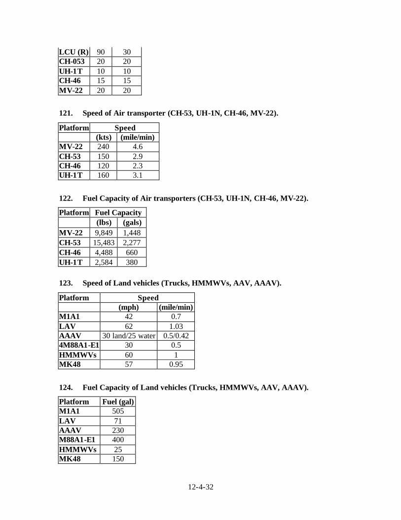
12-4-32
LCU (R) 90 30 CH-053 20 20 UH-1T 10 10 CH-46 15 15 MV-22 20 20
121. Speed of Air transporter (CH-53, UH-1N, CH-46, MV-22).
Platform Speed (kts) (mile/min) MV-22 240 4.6 CH-53 150 2.9 CH-46 120 2.3 UH-1T 160 3.1
122. Fuel Capacity of Air transporters (CH-53, UH-1N, CH-46, MV-22).
Platform Fuel Capacity (lbs) (gals) MV-22 9,849 1,448 CH-53 15,483 2,277 CH-46 4,488 660 UH-1T 2,584 380
123. Speed of Land vehicles (Trucks, HMMWVs, AAV, AAAV).
Platform Speed (mph) (mile/min) M1A1 42 0.7 LAV 62 1.03 AAAV 30 land/25 water 0.5/0.42 4M88A1-E1 30 0.5 HMMWVs 60 1 MK48 57 0.95
124. Fuel Capacity of Land vehicles (Trucks, HMMWVs, AAV, AAAV).
Platform Fuel (gal) M1A1 505 LAV 71 AAAV 230 M88A1-E1 400 HMMWVs 25 MK48 150
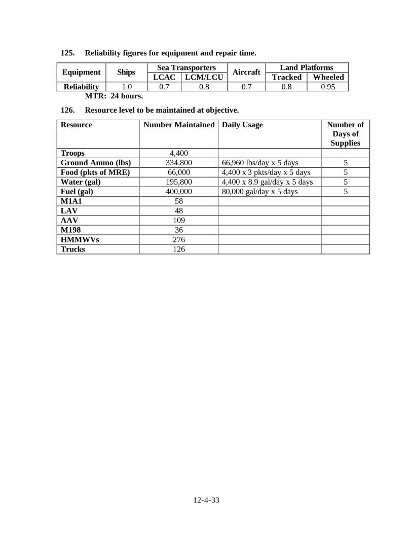
12-4-33
125. Reliability figures for equipment and repair time.
Sea Transporters Land Platforms Equipment Ships LCAC LCM/LCU
Aircraft Tracked Wheeled
Reliability 1.0 0.7 0.8 0.7 0.8 0.95 MTR: 24 hours.
126. Resource level to be maintained at objective.
Resource Number Maintained Daily Usage Number of Days of Supplies
Troops 4,400 Ground Ammo (lbs) 334,800 66,960 lbs/day x 5 days 5 Food (pkts of MRE) 66,000 4,400 x 3 pkts/day x 5 days 5 Water (gal) 195,800 4,400 x 8.9 gal/day x 5 days 5 Fuel (gal) 400,000 80,000 gal/day x 5 days 5 M1A1 58 LAV 48 AAV 109 M198 36 HMMWVs 276 Trucks 126

12-4-34
User Input – Distances Based on Burma Scenario (Miles)
CONUS (San Diego)
(1)
Fwd Deploy Forces (Japan)
(2)
Offshore Base (Diego Garcia)
(3)
Assembly Area (>250 NM)
(4)
Launching Area/Sea Base
(>50 NM) (5)
Landing Beach (6)
Iron Mountain (Chaungzon)
(7)
Objective (Mawlamyine)
(8)
CONUS (San Diego)
(1) 8,630 11,222 8,100 8,330 8,377 8,380 8,387
Fwd Deploy Forces (Japan)
(2)
2,373 7,574 7,804 7,854 7,854 7,861
Offshore Base (Diego Garcia)
(3) 2,032 2,262 2,323 2,326 2,319
Assembly Area (>250 NM)
(4) 230 278 281 288
Launching Area/Sea Base
(>50 NM) (5)
51 58
Landing Beach
(6)
3 10
Iron Mountain (Chaungzon)
(7)
7
Fro
m
Objective (Mawlamyine)
(8)
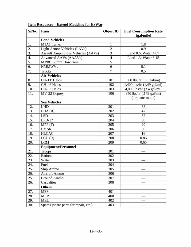
12-4-35
Item Resources – Extend Modeling for ExWar
S/No. Items Object ID Fuel Consumption Rate (gal/mile)
Land Vehicles 1. M1A1 Tanks 1 1.8 2. Light Armor Vehicles (LAVs) 2 0.9 3. Assault Amphibious Vehicles (AAVs) 3 Land 0.6; Water 4.07 4. Advanced AAVs (AAAVs) 4 Land 1.3; Water 6.15 5. M198 155mm Howitzers 5 0 6. HMMWVs 6 0.1 7. Trucks 7 0.5 Air Vehicles 8. UH-1T Helos 101 800 lbs/hr (.85 gal/mi) 9. CH-46 Helos 102 1,400 lbs/hr (1.49 gal/mi) 10. CH-53 Helos 103 4,000 lbs/hr (3.4 gal/mi) 11. MV-22 Osprey 106 350 lbs/hr (.179 gal/mi)
(airplane mode) Sea Vehicles 12. LHD 201 38 13. LHA (R) 202 47 14. LSD 203 32 15. LPD-17 204 30 16. MPF (F) 205 90 17. LMSR 206 90 18. HLCAC 207 16 19. LCU (R) 208 0.86 20. LCM 209 0.65 Equipment/Personnel 21. Troops 301 — 22. Rations 302 — 23. Water 303 — 24. Fuel 304 — 25. Ship Ammo 305 — 26. Aircraft Ammo 306 — 25. Ground Ammo 307 — 26. Casualties 308 — Others 27. MEF 401 — 28. MEB 400 — 29. MEU 402 — 30. Spares (spare parts for repair, etc.) 403 —
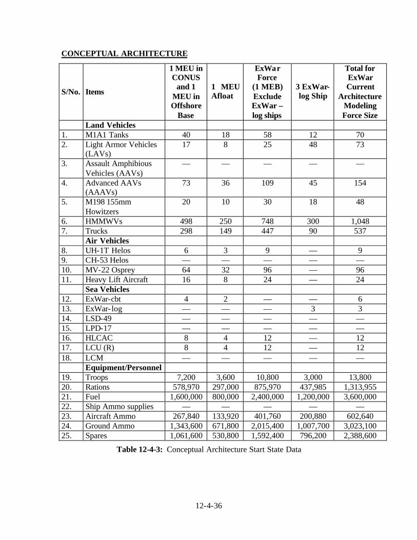
12-4-36
CONCEPTUAL ARCHITECTURE
S/No. Items
1 MEU in CONUS
and 1 MEU in Offshore
Base
1 MEU Afloat
ExWar Force
(1 MEB) Exclude ExWar –log ships
3 ExWar-log Ship
Total for ExWar Current
Architecture Modeling Force Size
Land Vehicles 1. M1A1 Tanks 40 18 58 12 70 2. Light Armor Vehicles
(LAVs) 17 8 25 48 73
3. Assault Amphibious Vehicles (AAVs)
— — — — —
4. Advanced AAVs (AAAVs)
73 36 109 45 154
5. M198 155mm Howitzers
20 10 30 18 48
6. HMMWVs 498 250 748 300 1,048 7. Trucks 298 149 447 90 537 Air Vehicles 8. UH-1T Helos 6 3 9 — 9 9. CH-53 Helos — — — — — 10. MV-22 Osprey 64 32 96 — 96 11. Heavy Lift Aircraft 16 8 24 — 24 Sea Vehicles 12. ExWar-cbt 4 2 — — 6 13. ExWar- log — — — 3 3 14. LSD-49 — — — — — 15. LPD-17 — — — — — 16. HLCAC 8 4 12 — 12 17. LCU (R) 8 4 12 — 12 18. LCM — — — — — Equipment/Personnel 19. Troops 7,200 3,600 10,800 3,000 13,800 20. Rations 578,970 297,000 875,970 437,985 1,313,955 21. Fuel 1,600,000 800,000 2,400,000 1,200,000 3,600,000 22. Ship Ammo supplies — — — — — 23. Aircraft Ammo 267,840 133,920 401,760 200,880 602,640 24. Ground Ammo 1,343,600 671,800 2,015,400 1,007,700 3,023,100 25. Spares 1,061,600 530,800 1,592,400 796,200 2,388,600
Table 12-4-3: Conceptual Architecture Start State Data
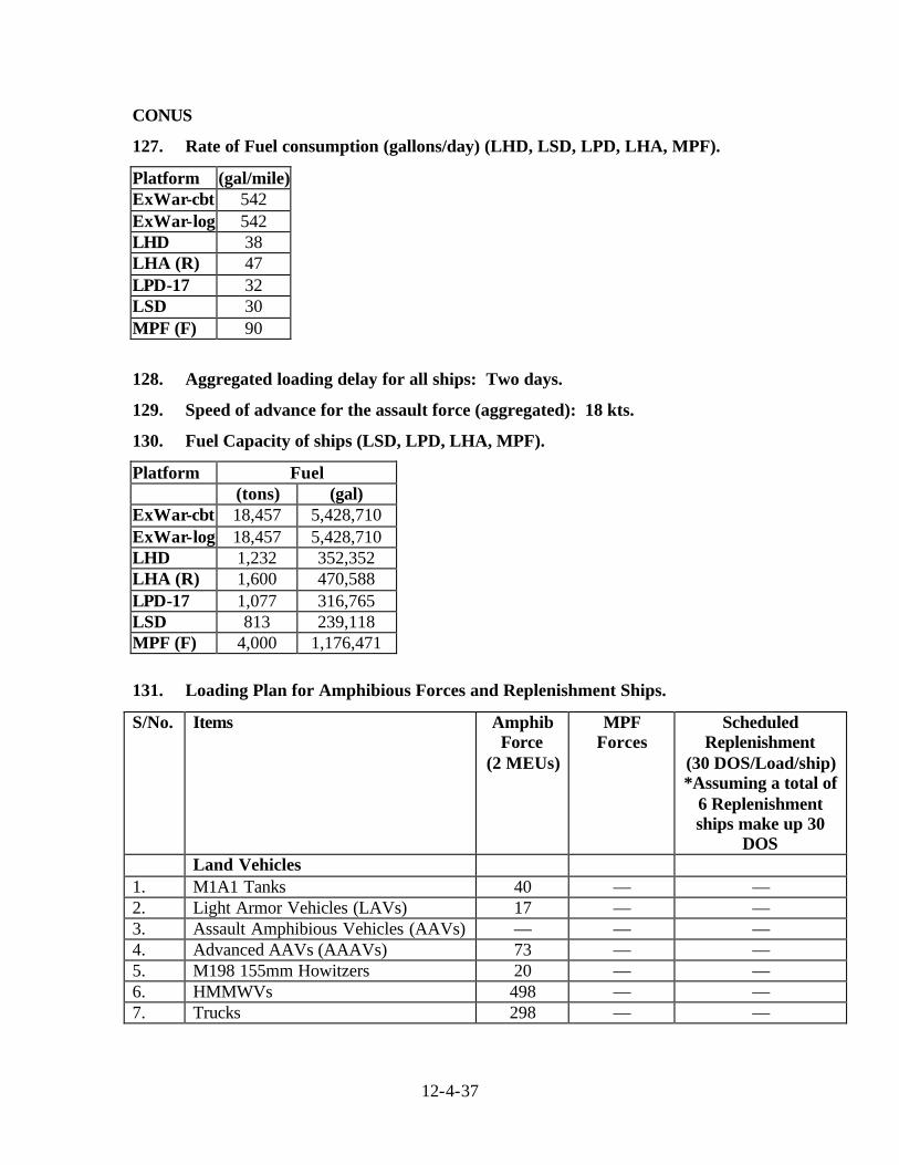
12-4-37
CONUS
127. Rate of Fuel consumption (gallons/day) (LHD, LSD, LPD, LHA, MPF).
Platform (gal/mile) ExWar-cbt 542 ExWar-log 542 LHD 38 LHA (R) 47 LPD-17 32 LSD 30 MPF (F) 90
128. Aggregated loading delay for all ships: Two days.
129. Speed of advance for the assault force (aggregated): 18 kts.
130. Fuel Capacity of ships (LSD, LPD, LHA, MPF).
Platform Fuel (tons) (gal) ExWar-cbt 18,457 5,428,710 ExWar-log 18,457 5,428,710 LHD 1,232 352,352 LHA (R) 1,600 470,588 LPD-17 1,077 316,765 LSD 813 239,118 MPF (F) 4,000 1,176,471
131. Loading Plan for Amphibious Forces and Replenishment Ships.
S/No. Items Amphib Force
(2 MEUs)
MPF Forces
Scheduled Replenishment
(30 DOS/Load/ship) *Assuming a total of
6 Replenishment ships make up 30
DOS Land Vehicles 1. M1A1 Tanks 40 — — 2. Light Armor Vehicles (LAVs) 17 — — 3. Assault Amphibious Vehicles (AAVs) — — — 4. Advanced AAVs (AAAVs) 73 — — 5. M198 155mm Howitzers 20 — — 6. HMMWVs 498 — — 7. Trucks 298 — —
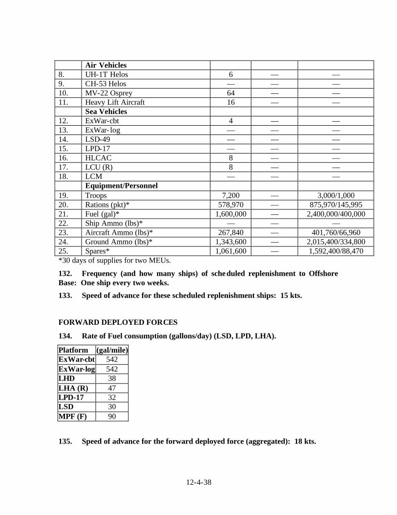
12-4-38
Air Vehicles 8. UH-1T Helos 6 — — 9. CH-53 Helos — — — 10. MV-22 Osprey 64 — — 11. Heavy Lift Aircraft 16 — — Sea Vehicles 12. ExWar-cbt 4 — — 13. ExWar- log — — — 14. LSD-49 — — — 15. LPD-17 — — — 16. HLCAC 8 — — 17. LCU (R) 8 — — 18. LCM — — — Equipment/Personnel 19. Troops 7,200 — 3,000/1,000 20. Rations (pkt)* 578,970 — 875,970/145,995 21. Fuel (gal)* 1,600,000 — 2,400,000/400,000 22. Ship Ammo (lbs)* — — — 23. Aircraft Ammo (lbs)* 267,840 — 401,760/66,960 24. Ground Ammo (lbs)* 1,343,600 — 2,015,400/334,800 25. Spares* 1,061,600 — 1,592,400/88,470 *30 days of supplies for two MEUs.
132. Frequency (and how many ships) of scheduled replenishment to Offshore Base: One ship every two weeks.
133. Speed of advance for these scheduled replenishment ships: 15 kts.
FORWARD DEPLOYED FORCES
134. Rate of Fuel consumption (gallons/day) (LSD, LPD, LHA).
Platform (gal/mile) ExWar-cbt 542 ExWar-log 542 LHD 38 LHA (R) 47 LPD-17 32 LSD 30 MPF (F) 90
135. Speed of advance for the forward deployed force (aggregated): 18 kts.
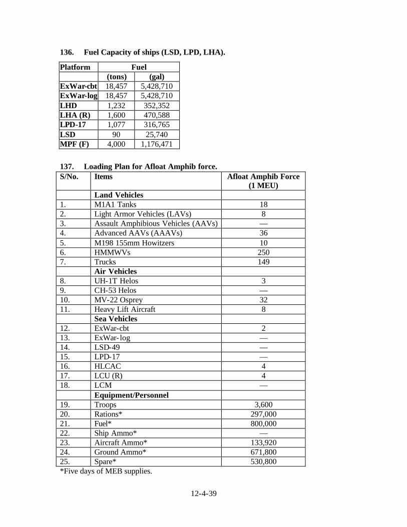
12-4-39
136. Fuel Capacity of ships (LSD, LPD, LHA).
Platform Fuel (tons) (gal) ExWar-cbt 18,457 5,428,710 ExWar-log 18,457 5,428,710 LHD 1,232 352,352 LHA (R) 1,600 470,588 LPD-17 1,077 316,765 LSD 90 25,740 MPF (F) 4,000 1,176,471 137. Loading Plan for Afloat Amphib force. S/No. Items Afloat Amphib Force
(1 MEU) Land Vehicles 1. M1A1 Tanks 18 2. Light Armor Vehicles (LAVs) 8 3. Assault Amphibious Vehicles (AAVs) — 4. Advanced AAVs (AAAVs) 36 5. M198 155mm Howitzers 10 6. HMMWVs 250 7. Trucks 149 Air Vehicles 8. UH-1T Helos 3 9. CH-53 Helos — 10. MV-22 Osprey 32 11. Heavy Lift Aircraft 8 Sea Vehicles 12. ExWar-cbt 2 13. ExWar- log — 14. LSD-49 — 15. LPD-17 — 16. HLCAC 4 17. LCU (R) 4 18. LCM — Equipment/Personnel 19. Troops 3,600 20. Rations* 297,000 21. Fuel* 800,000 22. Ship Ammo* — 23. Aircraft Ammo* 133,920 24. Ground Ammo* 671,800 25. Spare* 530,800 *Five days of MEB supplies.
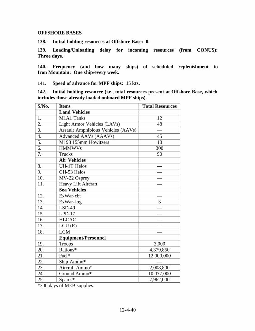
12-4-40
OFFSHORE BASES
138. Initial holding resources at Offshore Base: 0.
139. Loading/Unloading delay for incoming resources (from CONUS): Three days.
140. Frequency (and how many ships) of scheduled replenishment to Iron Mountain: One ship/every week.
141. Speed of advance for MPF ships: 15 kts.
142. Initial holding resource (i.e., total resources present at Offshore Base, which includes those already loaded onboard MPF ships).
S/No. Items Total Resources Land Vehicles 1. M1A1 Tanks 12 2. Light Armor Vehicles (LAVs) 48 3. Assault Amphibious Vehicles (AAVs) — 4. Advanced AAVs (AAAVs) 45 5. M198 155mm Howitzers 18 6. HMMWVs 300 7. Trucks 90 Air Vehicles 8. UH-1T Helos — 9. CH-53 Helos — 10. MV-22 Osprey — 11. Heavy Lift Aircraft — Sea Vehicles 12. ExWar-cbt — 13. ExWar- log 3 14. LSD-49 — 15. LPD-17 — 16. HLCAC — 17. LCU (R) — 18. LCM — Equipment/Personnel 19. Troops 3,000 20. Rations* 4,379,850 21. Fuel* 12,000,000 22. Ship Ammo* — 23. Aircraft Ammo* 2,008,800 24. Ground Ammo* 10,077,000 25. Spares* 7,962,000 *300 days of MEB supplies.
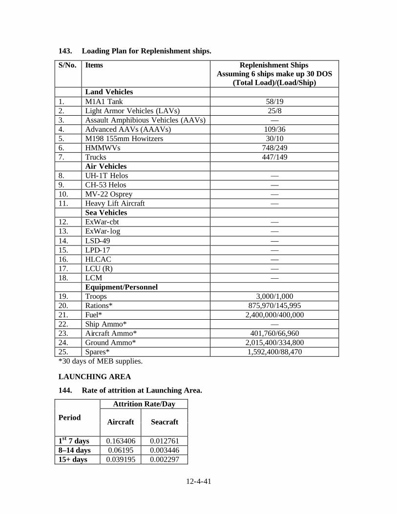
12-4-41
143. Loading Plan for Replenishment ships.
S/No. Items Replenishment Ships Assuming 6 ships make up 30 DOS
(Total Load)/(Load/Ship) Land Vehicles 1. M1A1 Tank 58/19 2. Light Armor Vehicles (LAVs) 25/8 3. Assault Amphibious Vehicles (AAVs) — 4. Advanced AAVs (AAAVs) 109/36 5. M198 155mm Howitzers 30/10 6. HMMWVs 748/249 7. Trucks 447/149 Air Vehicles 8. UH-1T Helos — 9. CH-53 Helos — 10. MV-22 Osprey — 11. Heavy Lift Aircraft — Sea Vehicles 12. ExWar-cbt — 13. ExWar- log — 14. LSD-49 — 15. LPD-17 — 16. HLCAC — 17. LCU (R) — 18. LCM — Equipment/Personnel 19. Troops 3,000/1,000 20. Rations* 875,970/145,995 21. Fuel* 2,400,000/400,000 22. Ship Ammo* — 23. Aircraft Ammo* 401,760/66,960 24. Ground Ammo* 2,015,400/334,800 25. Spares* 1,592,400/88,470 *30 days of MEB supplies.
LAUNCHING AREA
144. Rate of attrition at Launching Area.
Attrition Rate/Day
Period Aircraft Seacraft
1st 7 days 0.163406 0.012761 8–14 days 0.06195 0.003446 15+ days 0.039195 0.002297
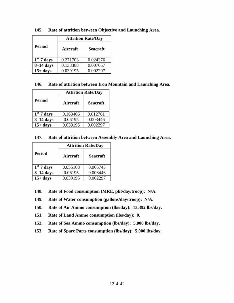
12-4-42
145. Rate of attrition between Objective and Launching Area.
Attrition Rate/Day
Period Aircraft Seacraft
1st 7 days 0.271703 0.024276 8–14 days 0.138388 0.007657 15+ days 0.039195 0.002297
146. Rate of attrition between Iron Mountain and Launching Area.
Attrition Rate/Day
Period Aircraft Seacraft
1st 7 days 0.163406 0.012761 8–14 days 0.06195 0.003446 15+ days 0.039195 0.002297
147. Rate of attrition between Assembly Area and Launching Area.
Attrition Rate/Day
Period Aircraft Seacraft
1st 7 days 0.055108 0.005743 8–14 days 0.06195 0.003446 15+ days 0.039195 0.002297
148. Rate of Food consumption (MRE, pkt/day/troop): N/A.
149. Rate of Water consumption (gallons/day/troop): N/A.
150. Rate of Air Ammo consumption (lbs/day): 13,392 lbs/day.
151. Rate of Land Ammo consumption (lbs/day): 0.
152. Rate of Sea Ammo consumption (lbs/day): 5,000 lbs/day.
153. Rate of Spare Parts consumption (lbs/day): 5,000 lbs/day.
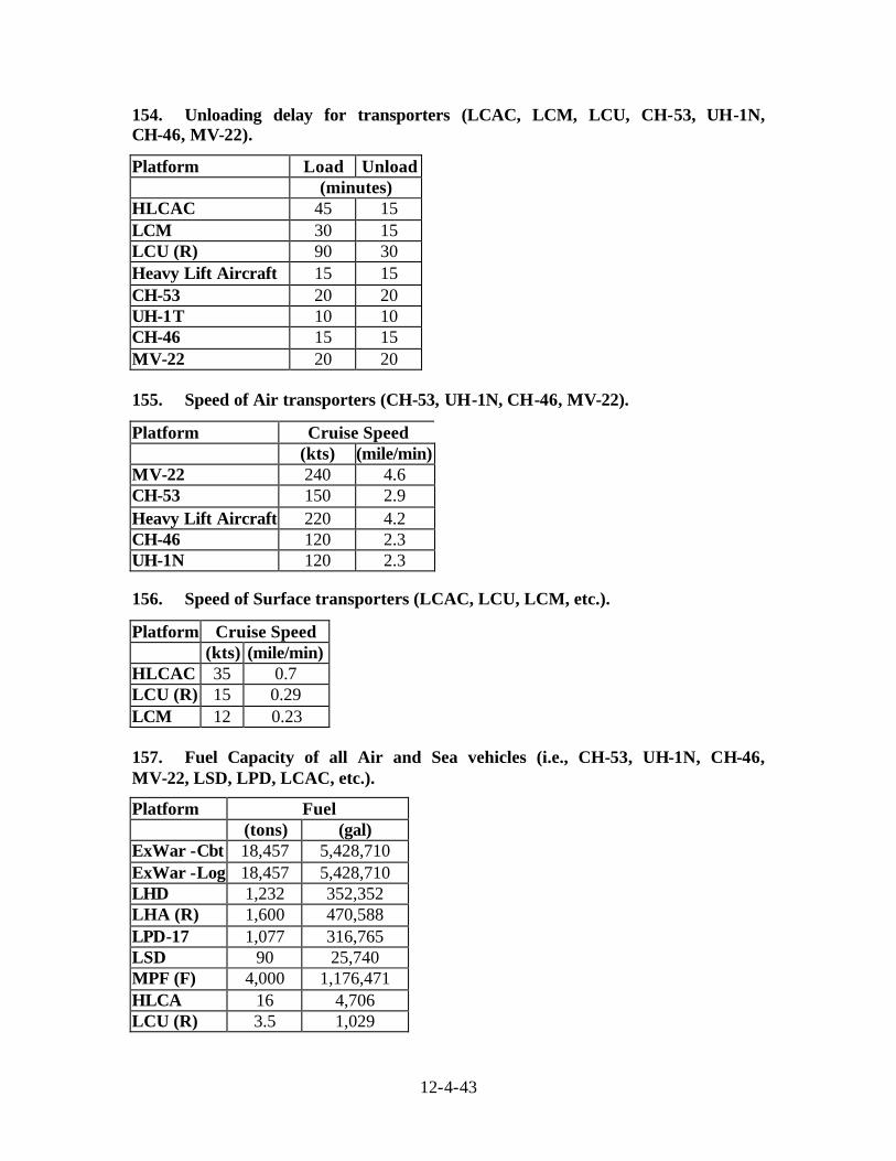
12-4-43
154. Unloading delay for transporters (LCAC, LCM, LCU, CH-53, UH-1N, CH-46, MV-22).
Platform Load Unload (minutes) HLCAC 45 15 LCM 30 15 LCU (R) 90 30 Heavy Lift Aircraft 15 15 CH-53 20 20 UH-1T 10 10 CH-46 15 15 MV-22 20 20 155. Speed of Air transporters (CH-53, UH-1N, CH-46, MV-22).
Platform Cruise Speed (kts) (mile/min) MV-22 240 4.6 CH-53 150 2.9 Heavy Lift Aircraft 220 4.2 CH-46 120 2.3 UH-1N 120 2.3
156. Speed of Surface transporters (LCAC, LCU, LCM, etc.).
Platform Cruise Speed (kts) (mile/min) HLCAC 35 0.7 LCU (R) 15 0.29 LCM 12 0.23 157. Fuel Capacity of all Air and Sea vehicles (i.e., CH-53, UH-1N, CH-46, MV-22, LSD, LPD, LCAC, etc.).
Platform Fuel (tons) (gal) ExWar -Cbt 18,457 5,428,710 ExWar -Log 18,457 5,428,710 LHD 1,232 352,352 LHA (R) 1,600 470,588 LPD-17 1,077 316,765 LSD 90 25,740 MPF (F) 4,000 1,176,471 HLCA 16 4,706 LCU (R) 3.5 1,029
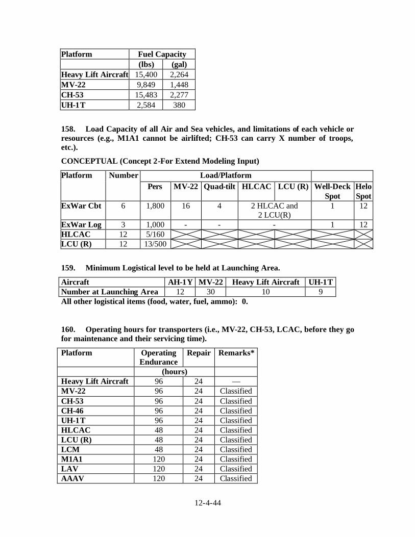
12-4-44
Platform Fuel Capacity (lbs) (gal) Heavy Lift Aircraft 15,400 2,264 MV-22 9,849 1,448 CH-53 15,483 2,277 UH-1T 2,584 380
158. Load Capacity of all Air and Sea vehicles, and limitations of each vehicle or resources (e.g., M1A1 cannot be airlifted; CH-53 can carry X number of troops, etc.).
CONCEPTUAL (Concept 2-For Extend Modeling Input)
Load/Platform Platform Number Pers MV-22 Quad-tilt HLCAC LCU (R) Well-Deck
Spot Helo Spot
ExWar Cbt 6 1,800 16 4 2 HLCAC and 2 LCU(R)
1 12
ExWar Log 3 1,000 - - - 1 12 HLCAC 12 5/160 LCU (R) 12 13/500
159. Minimum Logistical level to be held at Launching Area.
Aircraft AH-1Y MV-22 Heavy Lift Aircraft UH-1T Number at Launching Area 12 30 10 9 All other logistical items (food, water, fuel, ammo): 0.
160. Operating hours for transporters (i.e., MV-22, CH-53, LCAC, before they go for maintenance and their servicing time).
Platform Operating Endurance
Repair Remarks*
(hours) Heavy Lift Aircraft 96 24 — MV-22 96 24 Classified CH-53 96 24 Classified CH-46 96 24 Classified UH-1T 96 24 Classified HLCAC 48 24 Classified LCU (R) 48 24 Classified LCM 48 24 Classified M1A1 120 24 Classified LAV 120 24 Classified AAAV 120 24 Classified
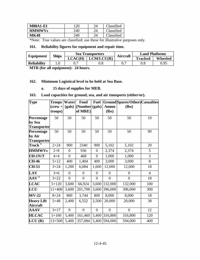
12-4-45
M88A1-E1 120 24 Classified HMMWVs 240 24 Classified MK48 240 24 Classified *Note: True values are classified; use these for illustrative purposes only.
161. Reliability figures for equipment and repair time.
Sea Transporters Land Platforms Equipment Ships LCAC(H) LCM/LCU(R)
Aircraft Tracked Wheeled
Reliability 1.0 0.7 0.8 0.7 0.8 0.95 MTR (for all equipment): 24 hours.
162. Minimum Logistical level to be held at Sea Base.
a. 15 days of supplies for MEB.
163. Load capacities for ground, sea, and air transports (either/or).
Type Troops (crew + troops)
Water (gals)
Food (Number of MRE)
Fuel (gals)
Ground Ammo (lbs)
Spares/Others (lbs)
Casualties
Percentage by Sea Transporter
50 50 50 50 50 50 10
Percentage by Air Transporter
50 50 50 50 50 50 90
Truck 1 2+24 900 2340 900 5,102 5,102 20 HMMWVs 2+8 0 936 0 2,374 2,374 5 UH-1N/T 4+4 0 468 0 1,000 1,000 3 CH-46 5+12 400 1,404 400 3,000 3,000 8 CH-53 3+24 1,200 6,084 1,600 12,000 12,000 18
LAV 3+6 0 0 0 0 0 4 AAV 2 3+22 0 0 0 0 0 18 LCAC 5+120 3,600 66,924 3,600 132,000 132,000 100 LCU 11+400 3,600 201,708 3,600 396,000 396,000 300
MV-22 8+24 800 3,744 800 8,000 8,000 18 Heavy Lift Aircraft
5+48 2,400 6,552 2,500 20,000 20,000 38
AAAV 3+17 0 0 0 0 0 12 HLCAC 5+160 5,400 161,460 5,400 316,800 316,800 120 LCU (R) 13+500 5,400 357,084 5,400 594,000 594,000 400
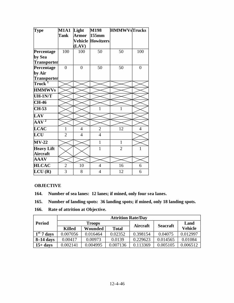
12-4-46
Type M1A1 Tank
Light Armor Vehicle (LAV)
M198 155mm Howitzers
HMMWVsTrucks
Percentage by Sea Transporter
100 100 50 50 100
Percentage by Air Transporter
0 0 50 50 0
Truck 1 HMMWVs UH-1N/T CH-46 CH-53 1 1
LAV AAV 2 LCAC 1 4 2 12 4 LCU 2 4 4
MV-22 1 1 Heavy Lift Aircraft
1 2 1
AAAV HLCAC 2 10 4 16 6 LCU (R) 3 8 4 12 6
OBJECTIVE
164. Number of sea lanes: 12 lanes; if mined, only four sea lanes.
165. Number of landing spots: 36 landing spots; if mined, only 18 landing spots.
166. Rate of attrition at Objective.
Attrition Rate/Day Troops Period
Killed Wounded Total Aircraft Seacraft Land
Vehicle 1st 7 days 0.007056 0.016464 0.02352 0.398154 0.04075 0.012997 8–14 days 0.00417 0.00973 0.0139 0.229623 0.014565 0.01084 15+ days 0.002141 0.004995 0.007136 0.113369 0.005105 0.006512
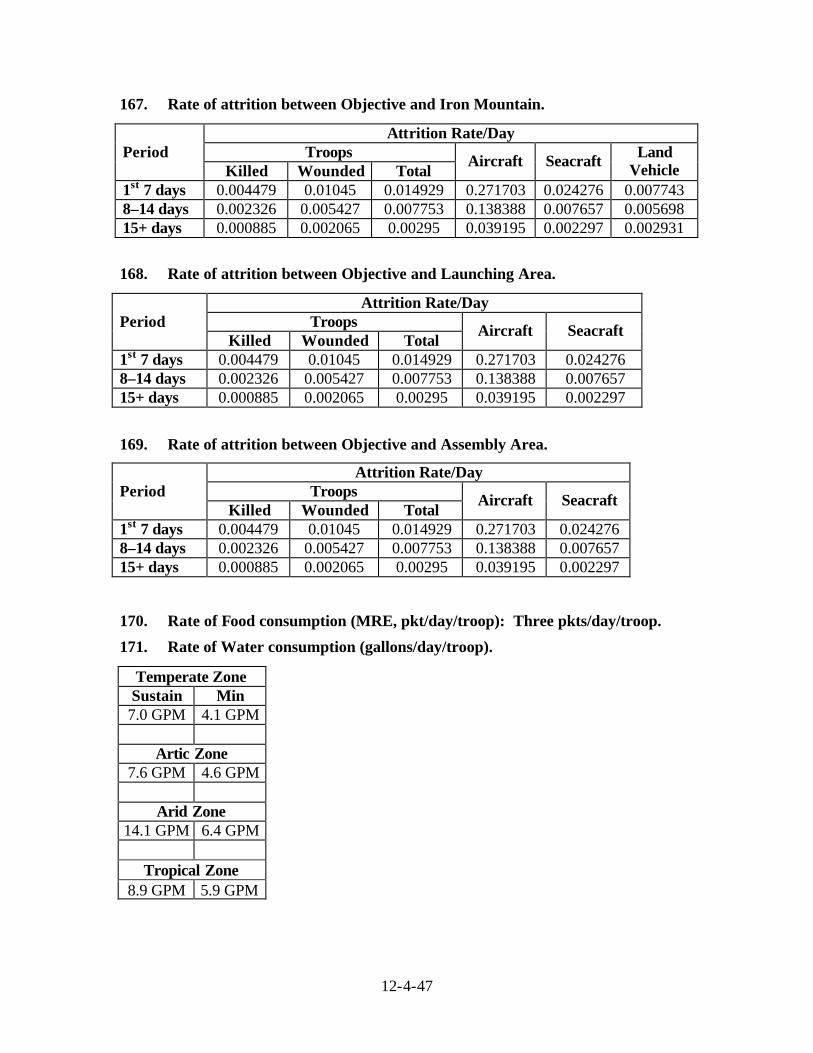
12-4-47
167. Rate of attrition between Objective and Iron Mountain.
Attrition Rate/Day Troops Period
Killed Wounded Total Aircraft Seacraft Land
Vehicle 1st 7 days 0.004479 0.01045 0.014929 0.271703 0.024276 0.007743 8–14 days 0.002326 0.005427 0.007753 0.138388 0.007657 0.005698 15+ days 0.000885 0.002065 0.00295 0.039195 0.002297 0.002931
168. Rate of attrition between Objective and Launching Area.
Attrition Rate/Day Troops Period
Killed Wounded Total Aircraft Seacraft
1st 7 days 0.004479 0.01045 0.014929 0.271703 0.024276 8–14 days 0.002326 0.005427 0.007753 0.138388 0.007657 15+ days 0.000885 0.002065 0.00295 0.039195 0.002297
169. Rate of attrition between Objective and Assembly Area.
Attrition Rate/Day Troops Period
Killed Wounded Total Aircraft Seacraft
1st 7 days 0.004479 0.01045 0.014929 0.271703 0.024276 8–14 days 0.002326 0.005427 0.007753 0.138388 0.007657 15+ days 0.000885 0.002065 0.00295 0.039195 0.002297
170. Rate of Food consumption (MRE, pkt/day/troop): Three pkts/day/troop.
171. Rate of Water consumption (gallons/day/troop).
Temperate Zone Sustain Min 7.0 GPM 4.1 GPM
Artic Zone
7.6 GPM 4.6 GPM Arid Zone
14.1 GPM 6.4 GPM
Tropical Zone 8.9 GPM 5.9 GPM
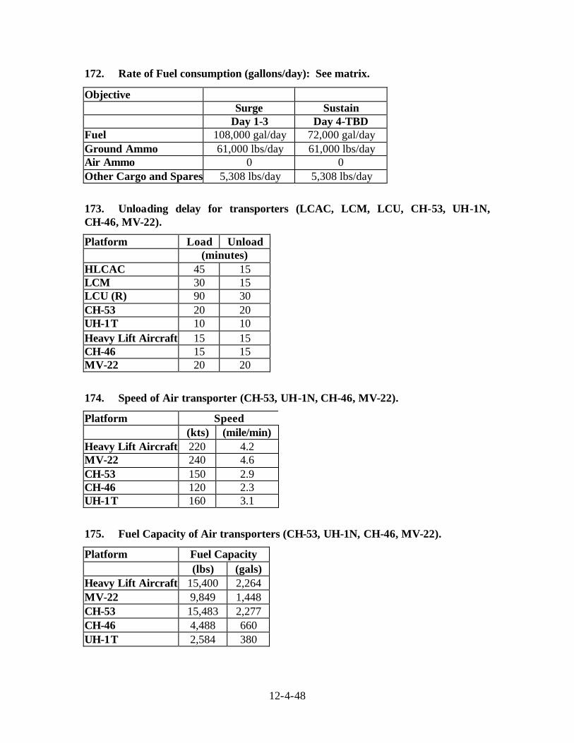
12-4-48
172. Rate of Fuel consumption (gallons/day): See matrix.
Objective Surge Sustain Day 1-3 Day 4-TBD Fuel 108,000 gal/day 72,000 gal/day Ground Ammo 61,000 lbs/day 61,000 lbs/day Air Ammo 0 0 Other Cargo and Spares 5,308 lbs/day 5,308 lbs/day
173. Unloading delay for transporters (LCAC, LCM, LCU, CH-53, UH-1N, CH-46, MV-22).
Platform Load Unload (minutes) HLCAC 45 15 LCM 30 15 LCU (R) 90 30 CH-53 20 20 UH-1T 10 10 Heavy Lift Aircraft 15 15 CH-46 15 15 MV-22 20 20
174. Speed of Air transporter (CH-53, UH-1N, CH-46, MV-22).
Platform Speed (kts) (mile/min) Heavy Lift Aircraft 220 4.2 MV-22 240 4.6 CH-53 150 2.9 CH-46 120 2.3 UH-1T 160 3.1
175. Fuel Capacity of Air transporters (CH-53, UH-1N, CH-46, MV-22).
Platform Fuel Capacity (lbs) (gals) Heavy Lift Aircraft 15,400 2,264 MV-22 9,849 1,448 CH-53 15,483 2,277 CH-46 4,488 660 UH-1T 2,584 380
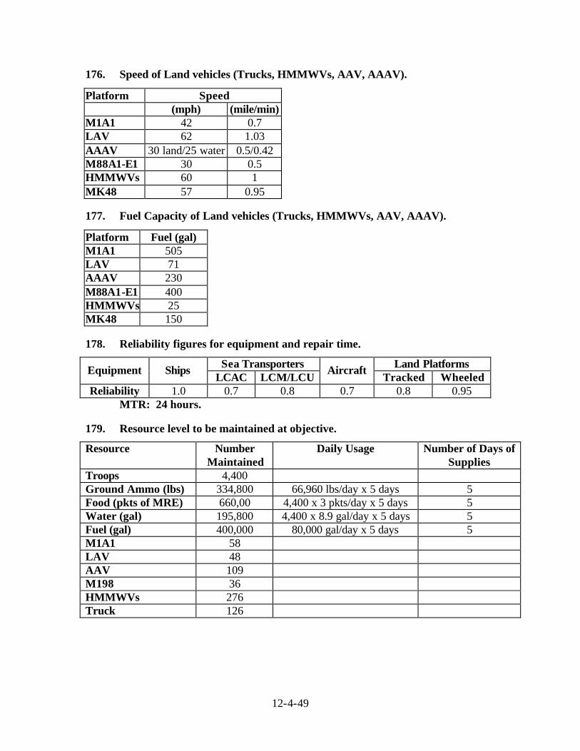
12-4-49
176. Speed of Land vehicles (Trucks, HMMWVs, AAV, AAAV).
Platform Speed (mph) (mile/min) M1A1 42 0.7 LAV 62 1.03 AAAV 30 land/25 water 0.5/0.42 M88A1-E1 30 0.5 HMMWVs 60 1 MK48 57 0.95 177. Fuel Capacity of Land vehicles (Trucks, HMMWVs, AAV, AAAV).
Platform Fuel (gal) M1A1 505 LAV 71 AAAV 230 M88A1-E1 400 HMMWVs 25 MK48 150 178. Reliability figures for equipment and repair time.
Sea Transporters Land Platforms Equipment Ships LCAC LCM/LCU
Aircraft Tracked Wheeled
Reliability 1.0 0.7 0.8 0.7 0.8 0.95 MTR: 24 hours.
179. Resource level to be maintained at objective.
Resource Number Maintained
Daily Usage Number of Days of Supplies
Troops 4,400 Ground Ammo (lbs) 334,800 66,960 lbs/day x 5 days 5 Food (pkts of MRE) 660,00 4,400 x 3 pkts/day x 5 days 5 Water (gal) 195,800 4,400 x 8.9 gal/day x 5 days 5 Fuel (gal) 400,000 80,000 gal/day x 5 days 5 M1A1 58 LAV 48 AAV 109 M198 36 HMMWVs 276 Truck 126
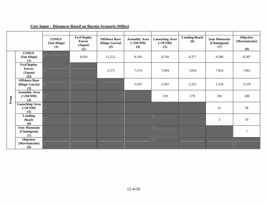
12-4-50
User Input – Distances Based on Burma Scenario (Miles)
CONUS (San Diego)
(1)
Fwd Deploy Forces (Japan)
(2)
Offshore Base (Diego Garcia)
(3)
Assembly Area (>250 NM)
(4)
Launching Area (>50 NM)
(5)
Landing Beach (6)
Iron Mountain (Chaungzon)
(7)
Objective (Mawlamyine)
(8)
CONUS (San Diego)
(1) 8,630 11,222 8,100 8,330 8,377 8,380 8,387
Fwd Deploy Forces (Japan)
(2))
2,373 7,574 7,804 7,854 7,854 7,861
Offshore Base (Diego Garcia)
(3) 2,032 2,262 2,323 2,326 2,319
Assembly Area (>250 NM)
(4) 230 278 281 288
Launching Area (>50 NM)
(5)
51 58
Landing Beach
(6)
3 10
Iron Mountain (Chaungzon)
(7)
7
Fro
m
Objective (Mawlamyine)
(8)
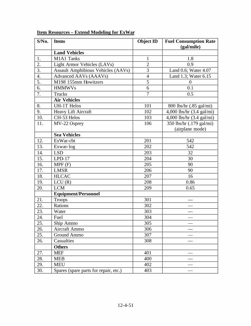
12-4-51
Item Resources – Extend Modeling for ExWar
S/No. Items Object ID Fuel Consumption Rate (gal/mile)
Land Vehicles 1. M1A1 Tanks 1 1.8 2. Light Armor Vehicles (LAVs) 2 0.9 3. Assault Amphibious Vehicles (AAVs) 3 Land 0.6; Water 4.07 4. Advanced AAVs (AAAVs) 4 Land 1.3; Water 6.15 5. M198 155mm Howitzers 5 0 6. HMMWVs 6 0.1 7. Trucks 7 0.5 Air Vehicles 8. UH-1T Helos 101 800 lbs/hr (.85 gal/mi) 9. Heavy Lift Aircraft 102 4,000 lbs/hr (3.4 gal/mi) 10. CH-53 Helos 103 4,000 lbs/hr (3.4 gal/mi) 11. MV-22 Osprey 106 350 lbs/hr (.179 gal/mi)
(airplane mode) Sea Vehicles 12. ExWar-cbt 201 542 13. Exwar- log 202 542 14. LSD 203 32 15. LPD-17 204 30 16. MPF (F) 205 90 17. LMSR 206 90 18. HLCAC 207 16 19. LCU (R) 208 0.86 20. LCM 209 0.65 Equipment/Personnel 21. Troops 301 — 22. Rations 302 — 23. Water 303 — 24. Fuel 304 — 25. Ship Ammo 305 — 26. Aircraft Ammo 306 — 25. Ground Ammo 307 — 26. Casualties 308 — Others 27. MEF 401 — 28. MEB 400 — 29. MEU 402 — 30. Spares (spare parts for repair, etc.) 403 —

APPENDIX 12-5
The ExWar DOE Matrix
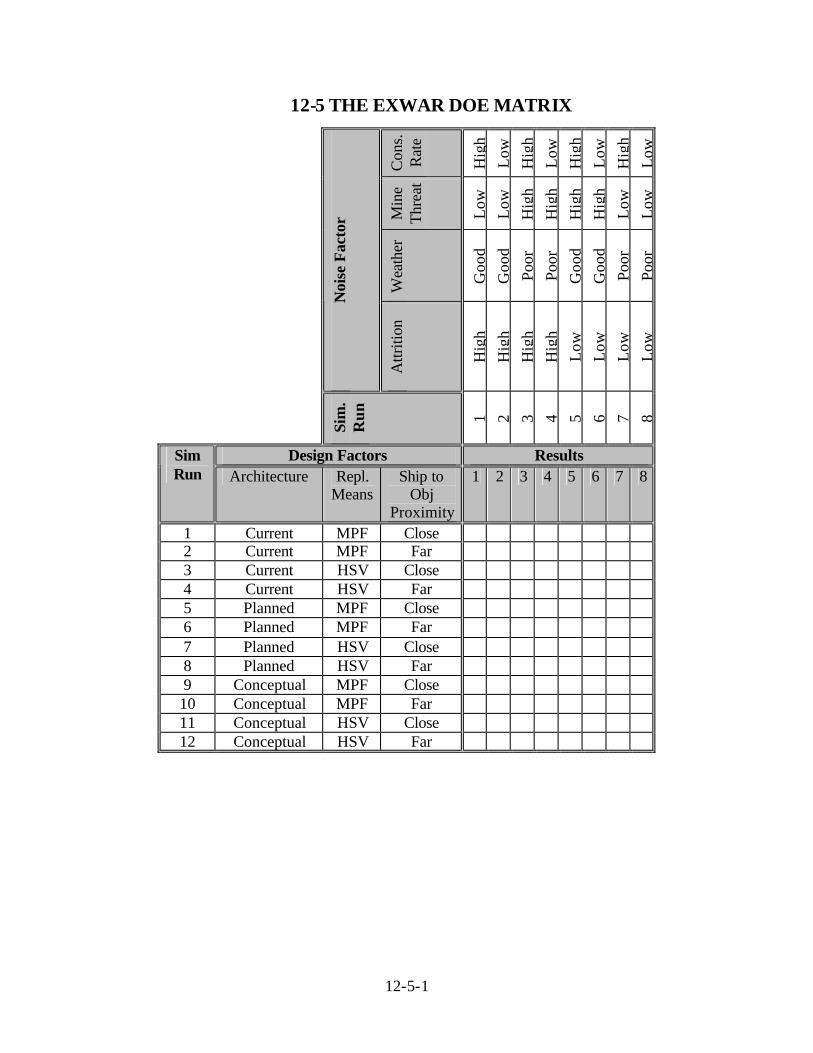
12-5-1
12-5 THE EXWAR DOE MATRIX
Con
s.
Rat
e
Hig
h L
ow
Hig
h L
ow
Hig
h L
ow
Hig
h L
ow
Min
e Th
reat
Low
L
ow
Hig
h H
igh
Hig
h H
igh
Low
L
ow
Wea
ther
Goo
d G
ood
Poor
Po
or
Goo
d G
ood
Poor
Po
or
Noi
se F
acto
r
Attr
ition
Hig
h H
igh
Hig
h H
igh
Low
L
ow
Low
L
ow
Sim
. R
un
1 2 3 4 5 6 7 8
Design Factors Results Sim Run Architecture Repl.
Means Ship to
Obj Proximity
1 2 3 4 5 6 7 8
1 Current MPF Close 2 Current MPF Far 3 Current HSV Close 4 Current HSV Far 5 Planned MPF Close 6 Planned MPF Far 7 Planned HSV Close 8 Planned HSV Far 9 Conceptual MPF Close
10 Conceptual MPF Far
11 Conceptual HSV Close
12 Conceptual HSV Far

APPENDIX 12-6
Design and Noise Factors
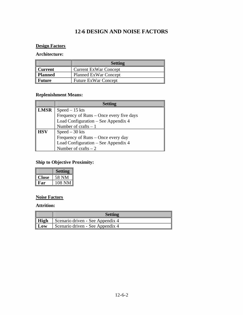
12-6-2
12-6 DESIGN AND NOISE FACTORS
Design Factors
Architecture:
Setting Current Current ExWar Concept Planned Planned ExWar Concept Future Future ExWar Concept
Replenishment Means:
Setting LMSR Speed – 15 kts
Frequency of Runs – Once every five days Load Configuration – See Appendix 4 Number of crafts – 1
HSV Speed – 30 kts Frequency of Runs – Once every day Load Configuration – See Appendix 4 Number of crafts – 2
Ship to Objective Proximity:
Setting Close 58 NM Far 108 NM
Noise Factors
Attrition:
Setting High Scenario driven - See Appendix 4 Low Scenario driven - See Appendix 4
12-6-3
Weather:
Setting Good Surface craft transit at input speed
Aircraft transit at input speed No increment in loading delay No reduction in sur face craft load capacity
Poor Surface craft transit speed reduced by 50% Aircraft transit speed reduced by 30%2 Air and Surface craft load times increased by 25% Surface craft load capacity reduced by 50%
Mine Threat:
Setting Low 12 landing lanes available High 4 landing lanes available
Consumption: (Ammo and Fuel)
Setting High Surge Rate Consumption for to be increased by 10 % for 10
days followed by Sustainment Rate through the rest of the campaign (see Appendix 4 for details of Sustainment Rate)
Low Surge Rate Consumption for 3 days followed by Sustainment Rate through the rest of the campaign (see Appendix 4 for details of Sustainment Rate)
2 In a moderate increment weather condition, aircraft’s effective transit speed is affected equally on both
way of transit, e.g., 25 kts faster on away leg (tail wind) and 25 kts slower on the return leg (head wind).
However, in increment weather, aircraft’s transit route is likely to be adjusted and would effectively be
longer. As such, the effective transit time will be longer. To model this effect on EXTENDTM, the aircraft
transit speed is reduced by a percentage.


![TABLE OF CONTENTS CHAPTER 1: PROVISIONS AND … · 2020-02-28 · MISSISSIPPI [TABLE OF CONTENTS CHAPTER 1: PROVISIONS AND RESPONSIBILITIES] Volume VI Chapter 1 1 Revised 12-01-14](https://img.pdfslide.net/doc/110x75/5eb2eaa08594fa09bd610e17/table-of-contents-chapter-1-provisions-and-2020-02-28-mississippi-table-of-contents.jpg)