Chapter 13Sampling distributions

Objectives (PSLS Chapter 13 & 14)Sampling distributions

Parameter versus statistic (Awards 27-31)

The law of large numbers (Law of Large Number Award, 28)

Sampling distributions (Sampling Distribution Award, 28)

Sampling distribution of the sample mean (Samp. Distribution Award)

The central limit theorem (Central Limits Theorem Award, 29)

x

Parameter versus statistic Sample: the part of the

population we actually examine

and for which we do have data.

A statistic is a number

summarizing a sample. We

often use a statistic to estimate

an unknown population

parameter.

Population: the entire group

of individuals in which we are

interested but usually can’t

assess directly.

A parameter is a number

summarizing the population.

Parameters are usually

unknown.

Population

Sample

The law of large numbers

Law of large numbers: As the number of randomly drawn observations

(n) in a sample increases,

the mean of the sample (x ̅) gets

closer and closer to the population

mean (quantitative variable).

the sample proportion ( ) gets

closer and closer to the population

proportion p (categorical variable).

p̂

Sampling distributions

Different random samples taken from the same population will give

different statistics. But there is a predictable pattern in the long run.

A statistic computed from a random sample is a random variable.

The sampling distribution of a statistic is the

probability distribution of that statistic for samples

of a given size n taken from a given population.

Note: When sampling randomly from a given population:

The law of large numbers describes what to expect if we took

samples of increasing size n.

A sampling distribution describes what would happen if we took

all possible random samples of a fixed size n.

Both are conceptual ideas with many important practical applications.

We rely on their well known mathematical properties, but we don’t

build actual sampling distributions when analyzing data.

The mean of the sampling distribution of x ̅ is μ.

There is no tendency for a sample average to fall systematically

above or below μ, even if the population distribution is skewed.

x� is an unbiased estimate of the population mean μ

assuming the samples are randomly chosen.

The standard deviation (σ) of the sampling distribution of x ̅

is σ/√n.

The standard deviation of the sampling distribution measures how

much the sample statistic x ̅ varies from sample to sample.

Averages are less variable than individual observations.

Sampling distribution of x ̅ (the sample mean)

For Normally distributed populations

When a variable in a population is Normally distributed, the sampling

distribution of the sample mean x ̅ is also Normally distributed.

population

Sample means

population N(μ σ)

↓

sampling distribution N(μ σ/√n)

Deer mice (Peromyscus maniculatus) have a body length (excluding the tail)

known to vary Normally, with a mean body length µ = 86 mm, and standard

deviation σ = 8 mm.

For random samples of 20 deer mice, the distribution of the sample mean body

length is approximately, 

A) Normal, mean 86, standard deviation 8 mm. 

B) Normal, mean 86, standard deviation 20 mm. 

C) Normal, mean 86, standard deviation 1.8 mm. 

D) Normal, mean 86, standard deviation 3.9 mm.

Standardizing a Normal sampling distribution (z)

N(0,1)

zxN(µ, σ/√n)

Here, we work with the sampling distribution,

and σ/√n is its standard deviation (indicative of spread).

Remember that σ is the standard deviation of the original population.

When the sampling distribution is Normal, we can standardize the

value of a sample mean x ̅ to obtain a z-score. This z-score can then be

used to find areas under the sampling distribution from Table B.

Hypokalemia is diagnosed when blood potassium levels are low, below

3.5mEq/dl. Let’s assume that we know a patient whose measured

potassium levels vary daily according to iid ~ N( = 3.8, = 0.2).

If only one measurement is made, what's the probability that this patient

will be diagnosed hypokalemic? Would this be a misdiagnosis?

The central limit theorem

Central limit theorem: When randomly sampling from any population

with mean and standard deviation , when n is large enough, the

sampling distribution of x ̅ is approximately Normal: N(μ σ/√n).

The larger the sample size n, the better the approximation of Normality.

This is very useful in inference: Many statistical tests assume Normality for

the sampling distribution. The central limit theorem tells us that, if the

sample size is large enough, we can safely make this assumption even if

the raw data appear non-Normal.

In many cases, n = 25 isn’t a huge sample. Thus,

even for strange population distributions we can

assume a Normal sampling distribution of the

sample mean, and work with it to solve problems!

How large a sample size?

It depends on the population distribution. More observations are

required if the population distribution is far from Normal.

A sample size of 25 or more is generally enough to obtain a Normal

sampling distribution from a skewed population, even with mild outliers in

the sample.

A sample size of 40 or more will typically be good enough to overcome an

extremely skewed population and mild (but not extreme) outliers in the

sample.

Population with strongly skewed distribution

Sampling distribution of for n = 2 observations

Sampling distribution of for n = 10 observations

Sampling distribution of for n = 25 observations

x

x

x

How do we know if the population is Normal or not? Sometimes we are told that a variable has an approximately Normal

distribution (e.g. large studies on human height or bone density).

Most of the time, we just don’t know. All we have is sample data.

We can summarize the data with a histogram and describe its shape and

estimate the likely magnitude of error. We can run simulations to quantify it.

If the sample is random, the shape of the histogram should be similar to the

shape of the population distribution.

The central limit theorem can help guess whether the sampling distribution

should look roughly Normal or not.

(a) Angle of big toe deformations

in 38 patients:

(b) Histogram of number of fruit

per day for 74 adolescent girls

Nu

mb

er o

f su

bje

cts

• Symmetrical, one small outlier• Population likely close to Normal• Sampling distribution ~ Normal

• Skewed, no outlier• Population likely skewed• Sampling distribution ~ Normal

given large sample size

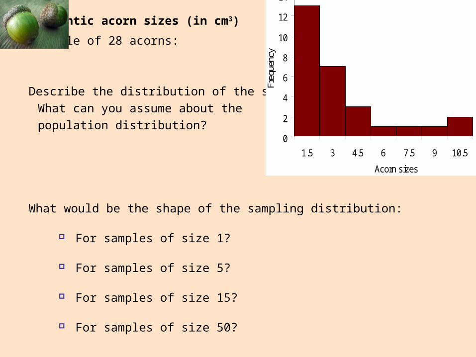
Atlantic acorn sizes (in cm3)

Sample of 28 acorns:

Describe the distribution of the sample.

What can you assume about the

population distribution?

What would be the shape of the sampling distribution:

For samples of size 1?

For samples of size 5?

For samples of size 15?

For samples of size 50?

0

2

4

6

8

10

12

14

1.5 3 4.5 6 7.5 9 10.5 More

Acorn sizes

Freq

uenc

y

Objectives (PSLS Chapter 14)

Estimation

Uncertainty and confidence (Margin of Error/CIs Award, 30)

Confidence intervals (Margin of Error/CIs Award, 30)

Uncertainty and confidence

If you picked different samples from a population, you would probably

get different sample means ( x̅ ) and virtually none of them would

actually equal the true population mean, .

nSample means,n subjects

n

Population, xindividual subjects

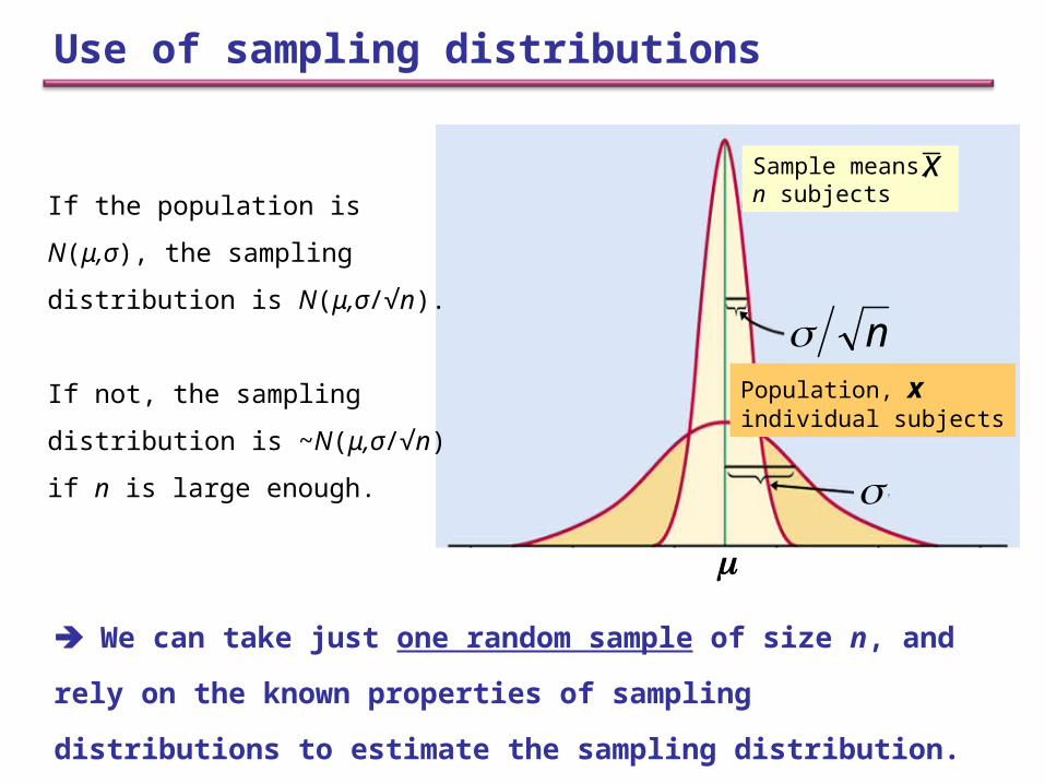
x If the population is N(μ,σ), the

sampling distribution is N(μ,σ/√n).

If not, the sampling distribution is

~N(μ,σ/√n) if n is large enough.

Use of sampling distributions

We can take just one random sample of size n, and rely on the

known properties of sampling distributions to estimate the

sampling distribution.

n

Blue dot: mean value of a given random sample

n

x ̅

~95% of all intervals computed with this

method capture the parameter μ.

Based on the ~68-95-99.7% rule, we

can expect that:

Red arrow: Interval of size plus or

minus 1.96*σ/√n

When we take a random sample, we

can compute the sample mean and an

interval of size plus-or-minus 2σ/√n

about the mean.

Confidence intervals

A confidence interval is a range of values with an associated

probability, or confidence level, C. This probability quantifies the

chance that the interval contains the unknown population parameter.

falls within the interval with probability (confidence level) C.

The confidence level C

(in %) represents an area

of corresponding size C

under the sampling

distribution.

mm

The margin of error, m

A confidence interval (“CI”) can be expressed as:

a center ± a margin of error: μ within x̅ ± m

an interval: μ within (x̅ − m) to (x ̅ + m)

The weight of single eggs varies Normally with standard deviation 5 g.

Think of a carton of 12 eggs as an SRS of size 12.

You buy one carton of 12 eggs. The average egg weight is x ̅ = 64.2g. What

can you infer about the mean µ of this population with roughly 95% confidence?

What is the distribution of the sample means ?

x

When taking a random sample from a Normal population with known

standard deviation σ, a level C confidence interval for µ is:

CI for a Normal population mean (σ known)

80% confidence level C

C

z* -z*

σ/√n is the standard deviation of

the sampling distribution

C is the area under the N(0,1)

between −z* and z*

* or x z n x m

How do we find z* values?

For 95% confidence level,

z* = 1.96 (almost 2)

(…)

We can use a table of z and t values

(Table C). For a given confidence

level C, the appropriate z* value is

listed in the same column.

Link between confidence level and margin of errorThe confidence level C determines the value of z* (in Table C).

The margin of error also depends on z*.

m z * n

C

Z*−Z*

m m

Higher confidence C implies a larger

margin of error m (less precision more

accuracy).

A lower confidence level C produces a

smaller margin of error m (more

precision less accuracy).

win/loose situation

Density of bacteria in solution

Measurement equipment has normal distribution with standard deviation

σ = 1 million bacteria/ml of fluid.

3 measurements: 24, 29, and 31 million bacteria/ml.

Mean: = 28 million bacteria/ml. Find the 99% and 90% CI.

x