CHAPTER 11:

Sampling Distributions

Lecture PowerPoint Slides

The Basic Practice of Statistics 6th Edition

Moore / Notz / Fligner

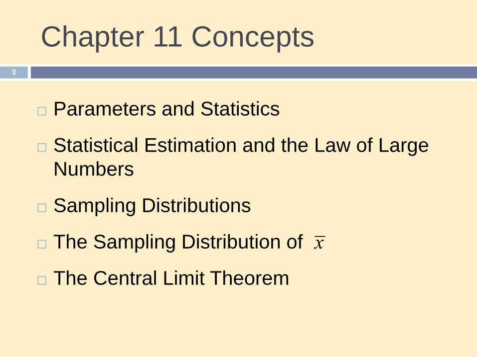
Chapter 11 Concepts 2

Parameters and Statistics

Statistical Estimation and the Law of Large

Numbers

Sampling Distributions

The Sampling Distribution of

The Central Limit Theorem

x

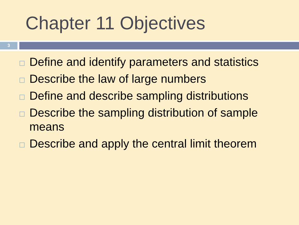
Chapter 11 Objectives 3

Define and identify parameters and statistics

Describe the law of large numbers

Define and describe sampling distributions

Describe the sampling distribution of sample

means

Describe and apply the central limit theorem

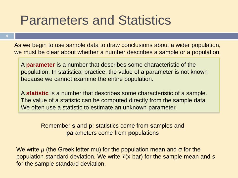
As we begin to use sample data to draw conclusions about a wider population,

we must be clear about whether a number describes a sample or a population.

Parameters and Statistics

A parameter is a number that describes some characteristic of the

population. In statistical practice, the value of a parameter is not known

because we cannot examine the entire population.

A statistic is a number that describes some characteristic of a sample.

The value of a statistic can be computed directly from the sample data.

We often use a statistic to estimate an unknown parameter.

Remember s and p: statistics come from samples and

parameters come from populations

4

x

We write µ (the Greek letter mu) for the population mean and σ for the

population standard deviation. We write (x-bar) for the sample mean and s

for the sample standard deviation.

5

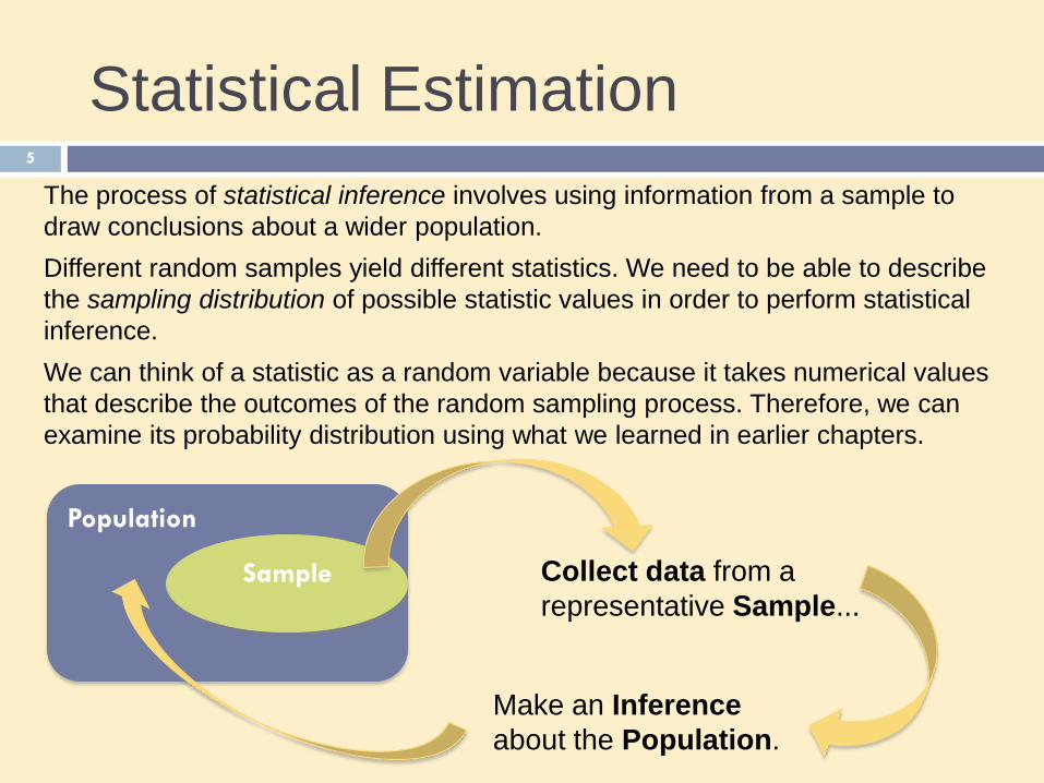
Statistical Estimation

The process of statistical inference involves using information from a sample to

draw conclusions about a wider population.

Different random samples yield different statistics. We need to be able to describe

the sampling distribution of possible statistic values in order to perform statistical

inference.

We can think of a statistic as a random variable because it takes numerical values

that describe the outcomes of the random sampling process. Therefore, we can

examine its probability distribution using what we learned in earlier chapters.

Population

Sample Collect data from a

representative Sample...

Make an Inference

about the Population.

6

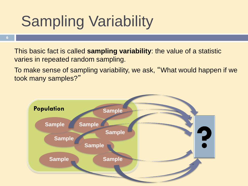
Sampling Variability

This basic fact is called sampling variability: the value of a statistic

varies in repeated random sampling.

To make sense of sampling variability, we ask, “What would happen if we

took many samples?”

Population

Sample

Sample

Sample

Sample

Sample

Sample

Sample

Sample

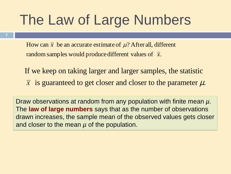
The Law of Large Numbers 7

Draw observations at random from any population with finite mean µ.

The law of large numbers says that as the number of observations

drawn increases, the sample mean of the observed values gets closer

and closer to the mean µ of the population.

. of valuesdifferent produce wouldsamples random

different all,After ? of estimate accuratean be can How

x

x

If we keep on taking larger and larger samples, the statistic

x is guaranteed to get closer and closer to the parameter m.

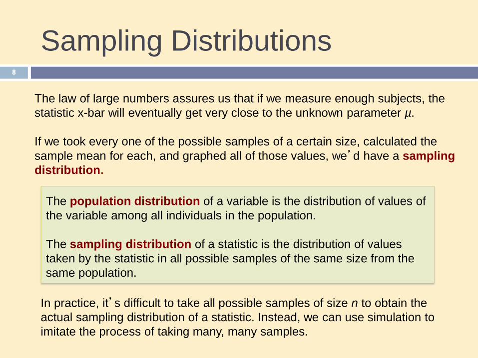
Sampling Distributions

The law of large numbers assures us that if we measure enough subjects, the

statistic x-bar will eventually get very close to the unknown parameter µ.

If we took every one of the possible samples of a certain size, calculated the

sample mean for each, and graphed all of those values, we’d have a sampling

distribution.

The population distribution of a variable is the distribution of values of

the variable among all individuals in the population.

The sampling distribution of a statistic is the distribution of values

taken by the statistic in all possible samples of the same size from the

same population.

In practice, it’s difficult to take all possible samples of size n to obtain the

actual sampling distribution of a statistic. Instead, we can use simulation to

imitate the process of taking many, many samples.

8

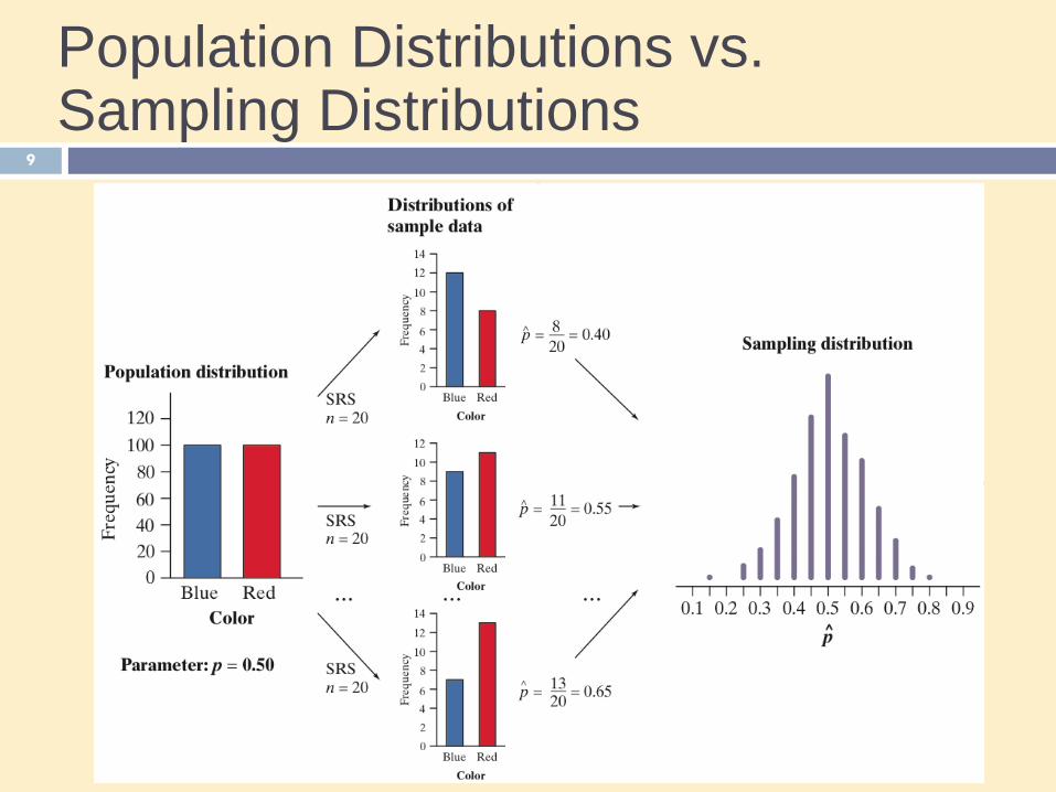
Population Distributions vs. Sampling Distributions

9

There are actually three distinct distributions involved when we

sample repeatedly and measure a variable of interest.

1)The population distribution gives the values of the variable

for all the individuals in the population.

2)The distribution of sample data shows the values of the

variable for all the individuals in the sample.

3)The sampling distribution shows the statistic values from

all the possible samples of the same size from the population.

10

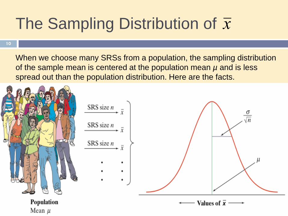
The Sampling Distribution of

When we choose many SRSs from a population, the sampling distribution

of the sample mean is centered at the population mean µ and is less

spread out than the population distribution. Here are the facts.

 

x

 

Note: These facts about the mean and standard deviation of x are true

no matter what shape the population distribution has.

The Sampling Distribution of Sample Means

 

The standard deviation of the sampling distribution of x is

s x =s

n

 

The mean of the sampling distribution of x is mx = m

 

Suppose that x is the mean of an SRS of size n drawn from a large population

with mean m and standard deviation s. Then :

If individual observations have the N(µ,σ) distribution, then the sample mean

of an SRS of size n has the N(µ, σ/√n) distribution regardless of the sample

size n.

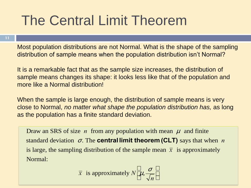
The Central Limit Theorem 11

Most population distributions are not Normal. What is the shape of the sampling

distribution of sample means when the population distribution isn’t Normal?

It is a remarkable fact that as the sample size increases, the distribution of

sample means changes its shape: it looks less like that of the population and

more like a Normal distribution!

When the sample is large enough, the distribution of sample means is very

close to Normal, no matter what shape the population distribution has, as long

as the population has a finite standard deviation.

Draw an SRS of size n from any population with mean m and finite

standard deviation s . The central limit theorem (CLT) says that when n

is large, the sampling distribution of the sample mean x is approximately

Normal:

x is approximately N m,s

n

æ

èç

ö

ø÷

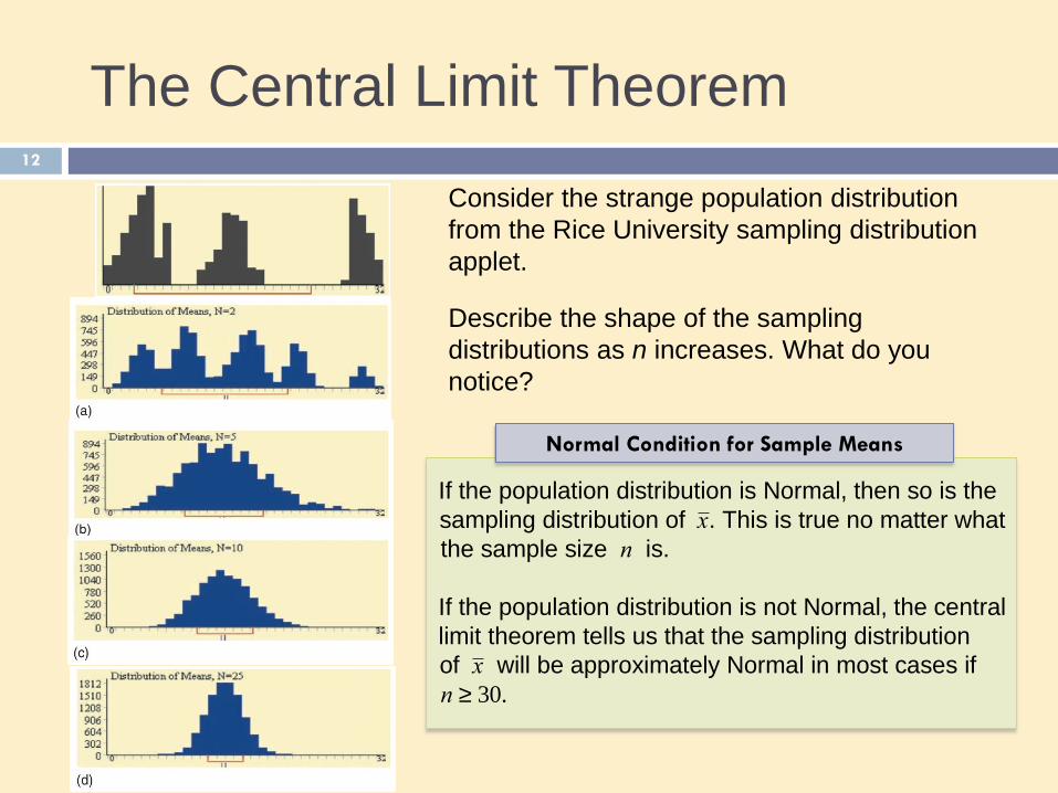
The Central Limit Theorem 12

Describe the shape of the sampling

distributions as n increases. What do you

notice?

Normal Condition for Sample Means

 

If the population distribution is Normal, then so is the

sampling distribution of x . This is true no matter what

the sample size n is.

If the population distribution is not Normal, the central

limit theorem tells us that the sampling distribution

of x will be approximately Normal in most cases if

n ³ 30.

Consider the strange population distribution

from the Rice University sampling distribution

applet.

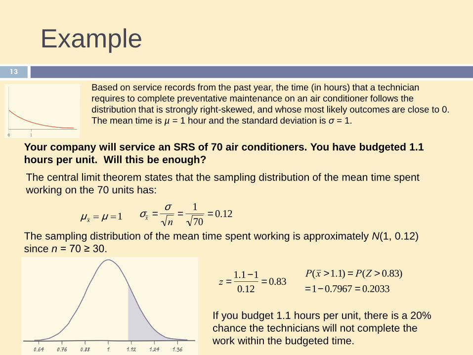
Example 13

Based on service records from the past year, the time (in hours) that a technician

requires to complete preventative maintenance on an air conditioner follows the

distribution that is strongly right-skewed, and whose most likely outcomes are close to 0.

The mean time is µ = 1 hour and the standard deviation is σ = 1.

Your company will service an SRS of 70 air conditioners. You have budgeted 1.1

hours per unit. Will this be enough?

1 μμ x

The central limit theorem states that the sampling distribution of the mean time spent

working on the 70 units has:

 

sx =s

n=

1

70= 0.12

The sampling distribution of the mean time spent working is approximately N(1, 0.12)

since n = 70 ≥ 30.

 

z =1.1 -1

0.12= 0.83

 

P(x >1.1) = P(Z > 0.83)

=1- 0.7967 = 0.2033

If you budget 1.1 hours per unit, there is a 20%

chance the technicians will not complete the

work within the budgeted time.

Chapter 11 Objectives Review 14

Define and identify parameters and statistics

Describe the law of large numbers

Define and describe sampling distributions

Describe the sampling distribution of sample

means

Describe and apply the central limit theorem