1

CHAPTER 17

THE OCTOPUS: MULTI-BUSINESS, GLOBAL COMPANIES If globalization has been a key theme of the last decade, it should come as no

surprise that the companies that we are valuing reflect that globalization. In this chapter,

we focus on a subset of companies that are diversified not only across countries, but also

across businesses. These multi-business firms, spread geographically, are difficult to

value because they represent multiple businesses, bundled and sold as a single package.

In this chapter, we examine these firms and consider the best ways of reflecting the

differences in risk, cash flow and growth characteristics across the different

businesses/regions that a company may operate in.

Multinationals The multinational, multi-business firm is not new to markets. At the risk of

arousing the ire of historians, we would argue that the colonial powers of previous

centuries – the British, the French and the Dutch – were the very first multi-national

businesses. In fact, the British were open about their commercial interests, allowing the

East India Company to treat entire countries as subsidiary businesses, from which it

generated profits and value. For much of the twentieth century, publicly traded firms

reflected this colonial history, with firms from developed markets in the United States

and Europe expanding into emerging markets. In the last decade, though, the equation has

been muddled by the emergence of multinational, emerging market companies that

operate in developed markets. In this section, we will examine the role that complex

companies play in the economy and then focus on some characteristics that they share.

Role in the economy

Many publicly traded firms in most markets are single-business companies that

derive the bulk of their revenues and earnings from domestic operations. While the firms

that are in many businesses and multiple markets that we highlight in this chapter may

not represent a large percentage of the overall number of firms, they have an outsized

influence, because they tend to be the largest firms (in terms of revenues, earnings and

market capitalization) in many markets.

2

The correlation between company size and operating in multiple businesses is not

an accident. After all, most firms that stay in a single business reach a saturation point in

that business sooner or later, and have to make a choice. They can accept the fact that

they are now mature companies and settle into that status, or they can aspire for more

growth, usually by entering new businesses and new markets. While not every large firm

is a General Electric or Siemens, most large firms have expanded beyond their original

markets (both in terms of products and geography). Finally, as economies mature,

companies within that economy that want to maintain high growth have to look at foreign

markets. Consequently, companies in Europe and North America have aggressively

expanded into emerging markets, in general, but Asia, in particular, because the potential

for economic growth is greatest in those markets.

Companies in emerging markets have historically not jumped on the bandwagon

of global growth, for two reasons. The first is that an Indian or Chinese company has

significant domestic demand, sustaining growth, and hence has less reason to look at

foreign markets. The other is that, at least until recently, the resources available to

emerging market companies were significantly more limited (both because of their size

and lack of access to capital markets) than those available to developed market

companies. In the last decade, as equity and debt markets have opened up in Asia and

Latin America, we have seen more emerging market companies emerge as global players.

This chapter is directed just as much at those companies, as it is at their developed market

counterparts.

Characteristics

In this section, we will focus on the shared characteristics of multi-business,

multinational companies, with the intent on unveiling some of the challenges that they

will create, when we value the firms:

1. Many different countries/markets: If the definition of a multinational firm is that it

operates in many markets, some in developed economies and some in emerging

eonomies, the consequences for valuation are straightforward. In the last chapter,

we noted that cash flows in emerging markets are riskier and should therefore be

discounted back at a higher discount rate than cash flows in developed markets.

3

For a firm that operates in only one emerging market, this would imply using a

higher discount rate for the expected cashflows. For firms operating in multiple

markets, the discount rates used to estimate value should be higher in some

markets (riskier emerging markets) than in others.

2. Risk parameters available for the aggregate but not for the pieces: If we treat a

multinational company as a portfolio of companies in different businesses and

market, we should be using a weighted average of the risk parameters for each of

the companies to estimate the risk for the consolidated company to derive its

value. The first problem we often encounter is that getting these risk parameters is

difficult, since the consolidated company (GE, Siemens) is the one that trades,

and not the individual pieces. The second problem is that as the weights on

businesses/countries change over time, as they will if the growth rates are

different, the weighted parameters have to be adjusted to reflect these changes.

3. Taxes reflect mix of marginal tax rates and jurisdictions: The marginal and

effective tax rates of a multinational reflect the different tax rates that the firm

pays on its different income, rather than the marginal tax rate of the domestic

market. In order to make a judgment of the tax rates to use in estimating cash

flows and discount rates, we have to not only look at where the company

generates its income, but also consider whether the firm can move its income into

lower tax locales and the consequences for tax rates.

4. Large centralized costs: As a company branches into multiple businesses and

many countries, it is inevitable that more and more costs will become centralized.

One reason for this tendency is control, as the firm tries to keep tabs on risk and

cash flows and to manage risk. The other is economies of scales, where the

replication of the same function (accounting and marketing, for instance) in

multiple divisions is avoided by having one company-wide accounting or

marketing department. The problem with centralized costs is not just the

magnitude of these expenses, but that these expenses then have to be allocated

across different businesses and regions, using some operating variable as a basis.

For instance, centralized G&A costs can be allotted to different divisions, based

upon revenues generated, and employee training and recruiting costs can be

4

divided up, based upon the number of employees in each division. While both

allocating mechanisms are reasonable, there is no way of checking what the actual

costs in each division are. Consequently, any earnings measures (EBITDA,

operating income or net income) computed at the divisional level or regional level

can be open to questioning.

5. Intra-company transactions: One troublesome aspect of firms that operate in many

regions and businesses is the prevalence of intra-company transactions. For

instance, a company that is in both iron ore mining and steel production will have

the steel business buying its raw material from the iron ore business. The former

will report the item as a cost and the latter as revenue and the company overall

will net the two items out. There are two consequences that can throw off

valuations. The first is that while the net income of the company may be

unaffected by these transactions, the revenues and costs will be inflated by the

volume of the trades. The second is that the prices at which these transactions are

arranged may be artificial, driven more by tax and control considerations than the

economics of the market place. After all, setting the price of iron ore too high

(relative to what you would have paid in the market) will lower the income for the

steel business but inflate the income for the mining business by exactly the same

amount. An analyst who tries to value just the mining business, based upon its

reported profits, will over estimate its value. The problems become worse when

the businesses provide financing for each other, as is the case when one division

lends money to another. Again, the interest rates set on the loan may not reflect

market rates, with the end result being a redistribution of profits across the

businesses. The presence of a financing arm within the company will exacerbate

this issue.

6. Complex holding structures: While not all multi-business, multinational

companies have complex holding structures, the structure of these firms lends

itself more readily to this problem. Multi-business companies often set up quasi-

independent or independent subsidiaries for some businesses, and then have

holdings in these subsidiaries that can be classified in a multitude of ways. For

instance, Coca Cola split off its bottling operations into an independent company

5

in the 1980s, and reduced its holding of that company to less than 50%, allowing

it to escape consolidation. In valuing Coca Cola, though, we have to also value

Coca Cola Bottling and attribute a proportion of that value to the parent company.

All of these characteristics affect the information that we use when valuing a company.

Valuation Issues When companies enter multiple businesses and many markets, we will confront

the issues in the inputs that we use to value a company. We can break down the problems

that we face, by looking at each category of inputs, first in discounted cash flow models,

and then in relative valuation.

Intrinsic (DCF) Valuation

The intrinsic or discounted cash flow value of a multi-business company is a

function of the same variables that determine the value of any company – the cash flows

from existing assets, the expected growth rate and value created by new assets, the risk in

these assets (as captured by a discount rate) and the period of time before the firm

becomes a stable growth firm.

a. Existing Assets: There are three problems with using aggregate earnings to value the

existing assets at a complex firm. The first is that the aggregate earnings come from

investments in very different businesses in different parts of the world, with currencies,

risk characteristics and capital investments varying widely across these investments.

Attaching one value to these earnings/cashflows becomes very difficult to do, because of

the differences in valuation fundamentals. Second, in those cases where companies do

break down earnings by business and region, they also have to provide additional detail

on capital expenditures and investments, which is often not forthcoming. Even the

earnings, broken down by division, are affected by allocation judgments made about

centralized costs. Figuring out which businesses get what benefits from these costs is

close to impossible to do. Finally, the presence of intra-company transactions and

financing can create a tangle of assets, earnings and book value that can easily lead to

some assets being double counted and others being ignored.

b. Growth Assets: As with existing earnings, not only can growth rates vary widely

across businesses and regions but the quality of growth can also be very different. To

6

make a good assessment of the value of growth, we need information on two key

variables – reinvestment amounts (and rates) by business and the returns generated on

capital invested in each. While obtaining this information for a single business company

is difficult enough, it is doubly so in complex companies where capital expenditures are

often aggregated at the company level and book values of capital at the divisions level are

either unavailable (because divisional balance sheets are not released) or not trustworthy

(because capital has been allocated to different businesses). Furthermore, as the firm

expands at different rates in different business and regions, the weighted growth rate will

change.

c. Discount Rates: If different businesses have different risk characteristics, and operating

in different parts of the world exposes companies to varying country risk, there are two

problems with assessing risk (and cost of capital) for a multi-business, global company.

The first is getting measures of risk for each part of the business, rather than for the firm

overall. The beta of GE as a company is not very useful in assessing the risk and value of

its aircraft business. The second is coming up with the weights to attach to each part of

the business to arrive at a risk measure for the entire firm. As the growth rates in different

businesses change, the weights will also shift. The other input into discount rates is

financial leverage, which is just as difficult to measure at the divisional level, both

because the debt used by the company is not broken down by division, and also because

the market value of equity is accessible only for the entire firm and not for individual

businesses. A final dilemma we face, both with discount rates and cash flows, is that a

multinational company will generate cash flows in different currencies and often issue

debt in multiple currencies. Since inflation rates, riskfree rates and discount rates can

vary by currency, we face a tangle of different estimates for the same input, depending on

which currency we use for the estimates.

d. Terminal value: When a firm is in multiple businesses, it is entirely likely that some of

these businesses are already in stable growth, whereas others are in high growth. If we

forecast cashflows until the entire firm is in stable growth, we will be forecasting

cashflows for mature businesses for extended periods. There is one added complication.

Firms can spin off, split off or divest businesses that they feel are being under valued by

the market, radically altering the make up of the firm in stable growth.

7

In summary, while the categories of inputs don’t change for multi-business companies,

there can be more estimation questions we face with each of them.

Relative Valuation

If the essence of relative valuation is finding other companies that look like your

company, and comparing how your company is priced relative to these comparable firms,

the problems with valuing a multi-business company that operates in many different

markets become obvious. Unless we find other companies that have a similar mix of

business and regional operations, which is a very unlikely scenario, we will be unable to

come up with comparable companies. Thus, there is no group of companies (or even a

single company) that we can call comparable, when valuing firms like General Electric or

Siemens.

Analysts who try to evade the problem by using comparable firms within each

business line will be stymied by the absence of market values for individual divisions and

information on commonly used scaling variables – earnings per share, operating income

and EBITDA. Assuming that we do find a way to allocate earnings to divisions and value

them, a final problem that we will have to deal with is the effect of consolidating multiple

businesses into one company. Thus, we have to determine whether to add a premium to

our estimated value (if we believe that the consolidation leads to cost savings or other

synergies) or attach a discount (if we believe that the consolidation results in lower

efficiency and a lack of corporate focus), and the magnitude of the adjustment.

The Dark Side of Valuation Given these valuation issues, analysts who value companies that have spread

across businesses and countries have adopted a combination of mechanisms, some of

which are acceptable compromises, given the absence of information, and some of which

can lead to valuation fiascos. In this section, we will focus on the latter.

Discounted Cash flow Valuation

In valuing multi-business, multinational companies, we face two challenges. One

is dealing with the different characteristics in terms of risk, cash flows and growth that

different businesses have, and the other is analyzing how to deal with different risk

8

exposures in different countries. In many cases, analysts choose to either assume that

using consolidated numbers will take care of the problem or to ignore the valuation issues

altogether.

Multi-country: Incorporation versus Operations

In the chapter on valuing emerging market companies, we noted that the focus on

where a company is incorporated often overwhelms any analysis of where it does

business. In the case of an emerging market company like Embraer, a Brazil-based

company with significant revenues from developed markets, this leads to an over

assessment of risk premiums and costs of equity and capital. With multinational

companies, the bulk of which are based in the United States and Europe, we see the

opposite problem. Since these companies are incorporated in developed markets, analysts

see no need to adjust for country or political risk, even though these firms may generate

large proportions of their revenues in emerging markets. In fact, the argument that

analysts use to defend this practice is that these companies, like Nestle and GE, are in so

many different regions of the world, that the country risk will be diversified away. As we

noted in chapter 16, this is wishful thinking, since emerging markets have become

increasingly correlated with each other.

The net effect of the practice of not adjusting discount rates of multinational

companies, that are based in developed markets, for risk, while allowing them to claim

credit for the growth and higher profits that they may be generating in emerging markets,

is that we will consistently over value these firms. For much of the 1980s and the 1990s,

analysts rewarded Coca Cola with a growth premium for its aggressive ventures into

emerging markets. It was only when confronted by a crisis, as Coca Cola was in the late

1990s by Russia’s internal turmoil, that they considered the additional risk in the strategy.

Multi-business: The averaging argument

It is not just risk that varies across businesses and markets, since every input into

a valuation model, including profit margins, returns on capital and growth rates, also

reflect the same characteristic. Some analysts stick with using the consolidated firm

figures for each of these inputs, arguing that they reflect the weighted average of the

multiple ventures that the firm is in. Technically, that is correct. However, the weights

9

that are reflected in the current values reflect the current values of the different businesses

and regions. To the extent that these weights may change over time, we should be

changing the inputs as well.

To illustrate, consider a multinational firm that reports an aggregate profit margin

of 8.4%, across two businesses and developed/emerging markets. Table 17.1 reflects the

weights that go into the computation:

Table 17.1: Revenue and Margin Breakdown

Developed Emerging Company Mining Profit Margin 12% 16% 14% Revenues ($) $150.00 $150.00 $300 Steel Profit Margin 4% 8% 6% Revenues ($) $450 $250 $700 Company Profit Margin 6% 11% 8.400% Revenues ($) $600 $400 $1,000

Now assume that the mining business is expanding at the rate of 20% a year, whereas the

steel business is growing only 5% a year, and that the much of the growth will come from

emerging markets. Given the profit margins by business and region, we can anticipate an

increase in profit margins over time for the consolidated company.

The point about averaging can be extended to every other input into the valuation.

The regression beta for a conglomerate, even if accurate today, will reflect the current

mix of businesses for the firm and will change over time, if these businesses grow at

different rates. Failing to adjust the estimates of these numbers for the future, for the

shifting weights, will generate distortions in value.

Ignoring Centralized Costs and Intra-company Transactions

In the last section, we noted the issues related to the allocation of centralized costs

and the effect of intra-company transactions on reported divisional earnings. Some

analysts, when valuing multi-national companies, choose to ignore both items, with

predictable consequences. For instance, ignoring centralized costs, while valuing

divisions based upon pre-allocation divisional earnings or revenues will lead to

significant over valuation. Alternatively, using post-allocation earnings at the divisional

level can lock into place any allocation errors that contaminated the earnings in the first

place. Similarly, failing to adjust revenues for intra-company transactions will lead us to

10

over estimate aggregate revenues for the consolidated company and potentially cash

flows in the future. If the intra-company transactions move profits from one division of a

firm to another, using divisional earnings will extend this problem into the forecasts of

divisional earnings and value.

Cross Holding valuations

As we noted in the last section, multinational, multi-business companies often

have complicated holding structures, with minority holdings in some subsidiaries and

majority holdings in others. In many cases, the information that is provided on the

subsidiaries, especially in the context of minority holdings, is too scanty to actually value

the subsidiaries. However, these firms often report an estimated value for the holdings on

the balance sheet, though that estimated value is not necessarily a market value or even a

fair value. When faced with multiple minority holdings, analysts often use these book

values as estimates of the intrinsic value of the holdings.

With majority holdings, analysts face a different problem. Since companies in

most countries are required to fully consolidate the subsidiaries’ numbers into their own –

100% of the subsidiaries’ operating earnings are counted as part of the parent company’s

earnings and 100% of the subsidiaries’ assets are recorded on the parent company’s

balance sheet – the portion of the subsidiary that does not belong to the parent company

is recorded as a liability (minority interest). Here again, the standard practice is to report

the book value of the minority interest, rather than the market value. In many discounted

cash flow valuations, analysts again reduce the value of the consolidated company by the

accounting estimate of minority interest, rather than the an estimate of the fair value.

In general, analysts valuing complex multi-business companies face large

information gaps. In many cases, they trust the managers of these companies to fill in the

gaps. To the extent that managers can provide misleading or optimistic estimates, these

numbers get fed into the final valuations.

Relative Valuation

The relative valuations of multi-business, multinational companies fall into two

groups – treating all multi-business companies as comparable and sum-of-the-parts

valuation.

11

a. Diversified companies sample: In this approach, analysts lump together all multi-

business companies and compare them to each other, even though they may

operate in widely different businesses and have very different weights on these

businesses. These valuations, in effect, assume that all diversified companies have

similar cashflow, growth and risk characteristics and should thus trade at similar

multiples of earnings or book value.

b. Sum-of-the-parts valuation: In this approach, which is more defensible, analysts

break the company down into individual businesses and then try to value each

business, based upon the pricing of comparable firms in that business. For

instance, they begin with the reported revenues or EBITDA for each business,

apply the average multiple at which publicly traded companies in that business

trade at to that number and treat the sum of the values as the value of the

consolidated company. The first factor that is overlooked here are the regional

differences in operations that may affect risk and growth, and through these, the

multiples. Thus, a US multinational that has an electronics business that derives

all of its revenues in China is still valued using comparable electronic companies

in the United States. The second factor that is missed or mis-valued is the

centralized cost. Valuing the individual businesses of a large conglomerate, by

applying multiples to revenues generated by each of the businesses, and ignoring

the billions of dollars in centralized costs will result in the unsurprising

conclusion that the firm will be worth more broken up, than as a consolidated

entity.

In summary, there is no easy way to value these complex companies using multiples and

comparables.

The Light Side of Valuation In the light side of valuation, we will explicitly allow for the challenges that we

have listed for complex companies and try to make the best estimates we can, given the

constraints of limited information.

12

Discounted Cashflow Valuation

To value firms that operate in multiple business and many regions, we will stick

with the standard framework of estimating cash flows and discount rates, but make

modifications to how we come up with the numbers along the way:

Step 1: Decide on whether to use aggregated or disaggregated numbers

The first step in the process is perhaps the most critical, since it will determine

how we approach the remaining steps. We have to decide, at the start of the process,

whether we intend to value the company as a whole (aggregated) or value its individual

businesses separately (disaggregated). In a world with no information or time constraints,

the choice would be an easy one. A disaggregated valuation should yield a better estimate

of value than an aggregated valuation. In practice, though, the choice will be complicated

by the following factors:

- Availability of information: The most critical variable determining whether we

value the company or individual businesses is access to information. To value a

company on an intrinsic basis, we need access to all of the operating details

(revenues, operating income and taxes), the financing breakdown (book values of

debt, equity and cash holdings, and market values of the same) and reinvestment

numbers (capital expenditures, working capital). There are very few companies

that provide this level of detail on individual businesses. One compromise

solution would be to substitute industry averages (for each business) where

information is lacking. Thus, we can use industry average working capital ratios

to determine expected investment in working capital for each business.

- Differences across businesses/ regions: The payoff to breaking a company down

into component parts is greatest when there are big differences across the parts, in

terms of risk, growth and profitability. Consider a multinational company that

operates only in the United States and Western Europe, and is in the specialty

retailing and apparel businesses. Since there is very little difference in country

risk across the regions that this firm operates in and only small differences in

profitability and growth in its two businesses, there will be little gained by

breaking it down into its individual parts and valuing it.

13

- Number of businesses/ regions: There is a pragmatic consideration that will also

determine whether or how much you want to disaggregate a company. If a firm

operates in 30 different businesses and 60 countries, we could, in theory, value

each of the 1800 parts (30 businesses X 60 countries) of the company separately,

but this is clearly not practical. In such cases, we may very well value the whole

company and hope that the law of averaging works in our favor.

As a final point, there is an intermediate solution, where we break the company down

into the parts that are most dissimilar from the rest of the company, while aggregating the

rest. With GE, for instance, we may value GE Capital separately from the rest of GE,

because it has fundamental differences with the rest of the company.

Step 2: Make a currency choice

Companies that operate in many countries have cash flows in multiple currencies.

In valuing these companies, we have to make a choice of which currency to build our

valuations around.

- Aggregated Valuation: When valuing the company as an aggregated whole, we

have no choice but to pick one currency as the base currency for estimation, since

you cannot have one discounted cashflow valuation, with different currency

choices underlying different estimates. Once that currency choice has been made,

all of the estimates (cash flows, growth rates and discount rates) have to be

consistent with that choice. Drawing on earlier discussion of riskfree rates in

different currencies, this requires us to build in the same expected inflation rate

into al of our estimates. While it is often easiest to work with the currency in

which the parent company reports its financial statements – US dollars for GE and

Coca Cola, for instance- there are two reasons why it may sometimes make sense

to switch to a different currency. The first is that the company has listings in many

markets and its financial reports in a different currency may be more

comprehensive or easier to work with than the domestic currency reports. Nestle,

for instance, has listing and reports financial statements in the UK and United

States, where its stock is listed, in addition to its Swiss listing, and provides more

information in its foreign listings than in its domestic listing. The second is that

14

getting inputs in the domestic currency for the company may be difficult to do.

Faced with the task of valuing a Russian multinational, we may very well find it

easier to value the company in US dollars than Russian rubles.

- Business valuations: With disaggregated valuation, you have more flexibility.

You can value each of the businesses, especially if they are located in different

regions of the world, in different currencies and do the conversion of the values at

the last step (when you add them to together), using the current exchange rates.

Alternatively, you can stick with a single currency in all of your valuations,

estimating cash flows and discount rates in that currency. In theory, there should

be no difference in the final value assessment, but given how difficult it is to work

with multiple currencies in a single company valuation, we believe that the latter

is less likely to be error prone.

Ultimately, the points we made about currency choice in earlier chapters continue to

apply. The value of a firm should not be a function of our currency choices. If it is, it is

because of inconsistencies in our forecasts.

Step 3: Estimate risk parameters, allowing for the multiple businesses/ regions that the

firm operates in.

Assessing risk in a multinational company that operates in many different

businesses is more difficult than it is for a company in a single business operating in a

single market. However, the measurement approaches that we developed in prior chapters

will stand us in good stead.

- Aggregated valuation: There are two keys to preserving valuation consistency in

aggregated valuations. The first is being cognizant of the differences in risk across

businesses and regions, when computing the cost of capital for a company that

operates in many businesses and multiple countries. The second is weighting these

different risk estimates appropriately, given the exposure of the firm to each one, to

estimate the risk parameters for the consolidated firm. Breaking down the inputs into

the cost of capital, we can generate the following implications:

o Betas: In the earlier chapters, we argued for the use of bottom up betas, i.e.

sector betas adjusted for financial leverage, on the basis that they are more

15

precise than regression betas. With multi-business companies, we can add

another benefit to using bottom up betas: the beta for a multi-business

company is a weighted average of the betas of the different businesses it

operates in. If we assume that estimating the sector betas, adjusted for

financial leverage, follows the same process here that it did in earlier chapters,

the one estimation challenge we face with companies that operate in many

businesses is in coming up with the weights for the businesses. One simple

solution is to base the weights on the revenues or earnings in each business, in

effect assuming that a dollar in revenues in one business is worth exactly the

same amount as revenues in a different business. An alternative is to estimate

an approximate value for each business, based perhaps upon revenues in that

business and the multiple of revenues that other publicly traded companies in

that business trade at.

o Risk premiums: In chapter 7, we argued that risk premiums should be higher

in emerging markets than in developed markets and presented ways in which

we could estimate the additional premium. In chapter 16, we looked at

emerging market companies and discussed how best to estimate the country

risk premiums and risk exposures of these companies. With multinational

companies, which derive some of their revenues from developed markets and

some from emerging markets, we face the same estimation issues that we did

with emerging market companies. We have to adjust the discount rate for the

exposure that multinationals have to emerging market risk. The simplest

adjustment to make is to compute equity risk premiums for every market that

a firm operates in and to take a weighted average of these numbers, using

revenues or operating income as the base. A more complex adjustment would

require that we compute lambdas (just as we did for emerging market

companies in chapter 16) for the multinational against each market, and use

these lambdas, in conjunction with country risk premiums, to compute the

cost of equity for a firm.

16

o Cost of debt: The cost of debt for a firm is computed by adding the default

spread to the riskfree rate and adjusting for any tax benefits generated by

interest expenses:

Cost of debt = (Riskfree Rate + Default Spread) (1- tax rate)

With multinational firms, there are three issues that we have to confront. The

first is the riskfree rate to use in computing the cost of debt can vary across the

different currencies in which the firms may actually borrow. This is a fairly

simple problem to resolve, since the riskfree rate to use will be determined by

the currency that you chose to do the valuation in step 2. In other words, if

you decide to do your valuation in US dollars, the riskfree rate will be the US

treasury bond rate, no matter what currency the actual borrowing is in. The

second is the default spread, which can vary widely across the different

borrowings of the firm. If the multinational firm has a rating, we can use the

rating to compute a default spread, which can then be added on to the riskfree

rate to compute the costs of debt. The final issue relates to the tax rate. While

it is the marginal tax rate that should be using the cost of debt, the reality is

that the marginal tax rates can vary across the different countries that the firm

operates in. One solution is to use the marginal tax rate of the country that the

multinational is incorporated in. An even better alternative is to use the

highest marginal tax rate, across the countries in which the company operates,

arguing that interest expenses will be directed to that country to maximize tax

benefits.

o Debt ratios: In keeping with our objective of valuing the consolidated firm,

the debt ratio we use will be based upon the aggregated debt for the entire

firm and the market value of all of its equity.

Using the bottom-up beta (estimated by taking a weighted average of the business

betas), the consolidated equity risk premium (reflecting the country risk exposure

created by operations), the cost of debt premised on the company’s overall default

risk and the debt ratio for the consolidated firm, we can obtain a cost of capital.

That number, though, will change over time as the firm’s mix of businesses shifts.

17

- Disaggregated valuations: When we value individual businesses, we obtain more

freedom in making out estimates, since the discount rates we use can vary widely

across the businesses. Again, using the inputs to the discount rate as a guide, we can

develop the following principles:

o Betas: When valuing individual businesses, we can use the bottom up betas

for those businesses in estimating the costs of equity. Since we are valuing

each business individually, there is no need to compute weighted averages of

the betas. For a firm with revenues from steel, mining and technology, we

would use the sector betas from each of these businesses in computing the

costs of equity for each business.

o Risk premiums: If we break businesses down by region and estimate each

part’s value separately, we should be estimating the cost of equity for each

region based upon the country risk premium for that region. In effect, we will

be valuing Coca Cola’s Russian operations, using the country risk premium

for Russia in the cost of equity computation and its Brazilian operations, using

the country risk premium for Brazil.

o Cost of debt: While we will stick with the principle that the cost of debt is the

sum of the riskfree rate and default spread, the costs of debt that we estimate

for the same company in different businesses/divisions can be different for

two reasons. One is that we may be using different currencies to value

different revenue streams; this can change the riskfree rate. The other is that

we can estimate different default spreads for different parts of the same

company, basing the spreads on the riskiness and the cash flows generated by

each part.

o Debt ratios: As with the other inputs into the cost of capital, the debt ratio can

vary across different pieces of the same firm. In some companies, where

individual divisions borrow money (rather than the consolidated firm), we

may be able to estimate these debt ratios based upon what firms actually do.

In most companies, where debt is consolidated at the company level, we have

two choices. The first is to assume that the company uses the same mix of

debt and equity across all businesses, and to use the debt ratio for the

18

company as the mix for every business. The second is to use the industry

average debt ratio for publicly traded firms in the same business and use this

debt ratio in computing costs of capital for individual businesses.

The bottom line: the cost of capital we use to discount cash flows in an aggregated

valuation represents the cost of capital for the consolidated firm, given the mix of

businesses and markets that it operates in, whereas the cost of capital we use to discount

cash flows in a disaggregated valuation represents the cost of capital of being in a

specific business in a specific country.

Step 4: Estimate future cash flows and value

Having picked a currency to do the valuation in and a discount rate that is

consistent with that currency choice, we have to estimate expected cash flows to value a

business. As with the prior sections, the way in which we approach this part of the

process will be determined in large part by whether we are valuing the consolidated firm

or its individual parts:

- Aggregated valuation: When we value a company on an aggregated basis, we have to

estimate the cash flows for the entire firm when valuing the firm. If we stick with

fundamentals for estimating growth in the cash flow, we will base the growth on the

combined reinvestment rate and return on capital for the entire firm. Given that the

firm operates in different businesses, with different reinvestment rates and returns on

capital in each, we are using a weighted average of the business specific values for

these numbers. As with the beta computation, we have to keep on eye on how the

weights shift over time and the implications for growth and cash flows.

- Disaggregated valuation: When valuing the individual parts of a larger company, we

acquire more flexibility. Rather than use a weighted average of the numbers across

the company, we can consider each business separately, assessing the reinvestment

rate and return on capital for that business as the basis for forecasting growth and

expected cash flows. With large conglomerates, we may very well find that some

businesses generate value from growth, by earning more than their cost of capital,

whereas other businesses within that same company destroy value, because the

returns on new investments are lower than the cost of capital.

19

In summary, as with the other inputs into valuation, disaggregated valuation requires

more of us (in terms of inputs) but also delivers more in terms of information.

Step 5: Get from firm value to equity value per share

To get from the value operating assets to equity value per share, we have to add

cash held by the firm, subtract out debt outstanding, add in the value of non-operating

assets, if any, and then divide by the numbers of shares. While the steps in this process

are identical for a multinational, multi-business, there can be significant estimation

questions at each stage of the process:

a. Add cash: In general, we would argue that a dollar in cash should be valued at a

dollar and that no discounts and premiums should be attached to cash, at least in the

context of an intrinsic valuation. There are two plausible scenarios where cash may be

discounted in value; in other words, a dollar in cash may be valued at less than a

dollar by the market.

• The first occurs when cash held by a firm is invested at a rate that is lower

than the market rate, given the riskiness of the investment. While most firms

in the United States can invest in government bills and bonds with ease today,

the options are much more limited for small businesses and in some markets

outside the United States. When this is the case, a large cash balance earning

less than a fair rate of return can destroy value over time.

• The management is not trusted with the large cash balance because of its past

track record on investments. While making a large investment in low-risk or

riskless marketable securities by itself is value neutral, a burgeoning cash

balance can tempt managers to accept large investments or make acquisitions

even if these investments earn sub-standard returns. In some cases, these

actions may be taken to prevent the firm from becoming a takeover target.1

To the extent that stockholders anticipate such sub-standard investments, the

current market value of the firm will reflect the cash at a discounted level. The

discount is likely to be largest at firms with few investment opportunities and

1 Firms with large cash balances are attractive targets, since the cash balance creduces an be used to offset some of the cost of making the acquisition.

20

poor management and there may be no discount at all in firms with significant

investment opportunities and good management.

b. Subtract out debt: With multinational firms, the debt that we net out to derive the

value of equity will depend in large part on what we are valuing. If we are valuing

equity in the consolidated firm, we will subtract out the market value of total debt

outstanding to estimate the value of equity. If on, the other hand, we are valuing

equity in individual businesses, we should be subtracting out the debt imputed for

these individual businesses.

c. Add in values of cross holdings: The way in which cross holdings are valued depends

upon the way the investment is categorized and the motive behind the investment. In

general, an investment in the securities of another firm can be categorized as a

minority, passive investment; a minority, active investment; or a majority, active

investment, and the accounting rules vary depending upon the categorization.

• Minority passive investments: If the securities or assets owned in another firm

represent less than 20% of the overall ownership of that firm, an investment is

treated as a minority, passive investment. These investments have an acquisition

value, which represents what the firm originally paid for the securities, and often

a market value. Accounting principles require that these assets be sub-categorized

into one of three groups – investments that will be held to maturity, investments

that are available for sale and trading investments. The valuation principles vary

for each.

a. For investments that will be held to maturity, the valuation is at historical cost

or book value and interest or dividends from this investment are shown in the

income statement.

b. For investments that are available for sale, the valuation is at market value,

but the unrealized gains or losses are shown as part of the equity in the

balance sheet and not in the income statement. Thus, unrealized losses reduce

the book value of the equity in the firm and unrealized gains increase the book

value of equity.

c. For trading investments, the valuation is at market value and the unrealized

gains and losses are shown in the income statement.

21

In general, firms have to report only the dividends that they receive from minority

passive investments in their income statements, though they are allowed an

element of discretion in the way they classify investments and, subsequently, in

the way they value these assets. This classification ensures that firms such as

investment banks, whose assets are primarily securities held in other firms for

purposes of trading, revalue the bulk of these assets at market levels each period.

This is called marking-to-market and provides one of the few instances in which

market value trumps book value in accounting statements.

• Minority, active investments: If the securities or assets owned in another firm

represent between 20% and 50% of the overall ownership of that firm, an

investment is treated as a minority, active investment. While these investments

have an initial acquisition value, a proportional share (based upon ownership

proportion) of the net income and losses made by the firm in which the

investment was made is used to adjust the acquisition cost. In addition, the

dividends received from the investment reduce the acquisition cost. This approach

to valuing investments is called the equity approach. The market value of these

investments is not considered until the investment is liquidated, at which point the

gain or loss from the sale, relative to the adjusted acquisition cost is shown as part

of the earnings in that period.

• Majority investments: If the securities or assets owned in another firm represent

more than 50% of the overall ownership of that firm, an investment is treated as a

majority active investment2. In this case, the investment is no longer shown as a

financial investment but is instead replaced by the assets and liabilities of the firm

in which the investment was made. This approach leads to a consolidation of the

balance sheets of the two firms, where the assets and liabilities of the two firms

are merged and presented as one balance sheet. The share of the firm that is

owned by other investors is shown as a minority interest on the liability side of

the balance sheet. A similar consolidation occurs in the other financial statements

of the firm as well, with the statement of cash flows reflecting the cumulated cash

2 Firms have evaded the requirements of consolidation by keeping their share of ownership in other firms below 50%.

22

inflows and outflows of the combined firm. This is in contrast to the equity

approach, used for minority active investments, in which only the dividends

received on the investment are shown as a cash inflow in the cash flow statement.

Here again, the market value of this investment is not considered until the

ownership stake is liquidated. At that point, the difference between the market

price and the net value of the equity stake in the firm is treated as a gain or loss

for the period.

Given that the holdings in other firms can be accounted for in three different ways, how

do you deal with each type of holding in valuation? The best way to incorporate each of

them is to value the equity in each holding separately and estimate the value of the

proportional holding. This would then be added on to the value of the equity of the parent

company. Thus, to value a firm with holdings in three other firms, you would value the

equity in each of these firms, take the percent share of the equity in each and add it to the

value of equity in the parent company. When income statements are consolidated, you

would first need to strip the income, assets and debt of the subsidiary from the parent

company’s financials before you do any of the above. If you do not do so, you will

double count the value of the subsidiary.

As a firm’s holdings become more numerous, estimating the values of individual

holdings will become more onerous. In fact, the information needed to value the cross

holdings may be unavailable, leaving analysts with less precise choices:

1. Market Values of Cross Holdings: If the holdings are publicly traded, substituting in

the market values of the holdings for estimated value is an alternative worth exploring.

While you risk building into your valuation any mistakes the market might be making in

valuing these holdings, this approach is more time efficient, especially when a firm has

dozens of cross holdings in publicly traded firms.

2. Estimated Market Values: When a publicly traded firm has a cross holding in a private

company, there is no easily accessible market value for the private firm. Consequently,

you might have to make your best estimate of how much this holding is worth, with the

limited information that you have available. There are a number of alternatives. One way

to do this is to estimate the multiple of book value at which firms in the same business (as

the private business in which you have holdings) typically trade at and apply this multiple

23

to the book value of the holding in the private business. . Assume for instance that you

are trying to estimate the value of the holdings of a pharmaceutical firm in 5 privately

held biotechnology firms, and that these holdings collectively have a book value of $ 50

million. If biotechnology firms typically trade at 10 times book value, the estimated

market value of these holdings would be $ 500 million. In fact, this approach can be

generalized to estimate the value of complex holdings, where you lack the information to

estimate the value for each holding or if there are too many such holdings. For example,

you could be valuing a Japanese firm with dozens of cross holdings. You could estimate a

value for the cross holdings by applying a multiple of book value to their cumulative

book value. Note that using the accounting estimates of the holdings, which is the most

commonly used approach in practice, should be a last resort, especially when the values

of the cross holdings are substantial.

Step 6: Decide whether you want to adjust the value of equity for other factors

Once we estimate the value of equity in a company with investments in multiple

businesses and markets, we have to consider whether (and if so, how) to adjust for other

factors that may affect equity value. The first adjustment is for the complexity of multi-

business companies, which makes them more difficult to value, thus leading to a discount

on estimated value. The second adjustment is a positive one, and reflects the likelihood

that the multi-business company will be split up into individual companies, and the value

increment that you expect to follow:

a. Complexity: Conventional valuation models have generally ignored complexity on

the simple premise that what we do not know about firms cannot hurt is in the

aggregate because it can be diversified away. In other words, we trust the managers

of the firm to tell us the truth what they earn, what they own and what they owe. Why

would they do this? If managers are long-term investors in the company, it is argued,

they would not risk their long term credibility and value for the sake of a short term

price gain (obtained by providing misleading information). While there might be

information that is not available to investors about these invisible assets, the risk

24

should be diversifiable and thus should not have an effect on value.3 This view of the

world is not irrational but it does run into two fundamental problems. First, managers

can take substantial short term profits by manipulating the numbers (and then

exercising options and selling their stock) which may well overwhelm whatever

concerns they have about long term value and credibility. Second, even managers

who are concerned about long term value may delude themselves into believing their

own forecasts, optimistic though they might be. It is not surprising, therefore, that

firms become sloppy during periods of sustained economic growth. Secure in the

notion that there will never be another recession (at least not in the near future), they

adopt aggressive accounting practices that overstate earnings. Investors, lulled by the

rewards that they generate by investing in stocks during these periods, accept these

practices with few questions. The downside of trusting managers is obvious. If

managers are not trustworthy and firms manipulate earnings, investors who buy stock

in complex companies are more likely to be confronted with negative surprises than

positive ones. This is because managers who hide information deliberately from

investors are more likely to hide bad news than good news. While these negative

surprises can occur at any time, they are more likely to occur when overall economic

growth slows (a recession!) and are often precipitated by a shock. We could do a

conventional valuation of a firm, using unadjusted cashflows, growth rates and

discount rates, and then apply a discount to this value to reflect the complexity of its

financial statements. But how would we quantify this complexity discount? There are

two options:

i. Apply a conglomerate discount: We could estimate the discount at which

complex firms trade at in the market place, relative to simpler firms. the last

two decades, evidence has steadily mounted that markets discount the value of

conglomerates, relative to single-business (or pure play) firms. In a study in

1999, Villalonga compared the ratio of market value to replacement cost

3 This follows from the assumption that managers are being honest. If this is the case, the information that is not available to investors has an equal chance of being good news and bad news. Thus, for every complex company that uncovers information that reduces its value, there should be another complex company where the information that comes out will increase value. In a diversified portfolio, these effects should average out to zero.

25

(Tobin’s Q) for diversified firms and specialized firms and reported that the

former traded at a discount of about 8% on the latter.4 Similar results were

reported in earlier studies.5

ii. Measure complexity directly and estimate a discount based on complexity: A

more sophisticated option is to use a complexity scoring system, to measure

the complexity of a firm’s financial statements and to relate the complexity

score to the size of the discount. Damodaran (2006) looks at different

measures of complexity, ranging from the number of pages in the SEC filings

of the company to a complexity scores that are computed from the information

in financial statements, and suggests ways of adjusting value for complexity.6

b. Potential restructuring: One question that overhangs every multi-business company is

whether the company would be worth more if it were broken up into independent

businesses. This, in fact, is the motivation behind the sum of the parts valuations that

we described in an earlier section. To the extent that a firm will be worth more as

separate parts, we may have to add a premium to value to reflect the probability that

the firm will be broken up and the value increment that will occur as a consequence.

Illustration 17.1: Valuing United Technologies – Aggregated Basis

United Technologies is a publicly traded company in the United States with

business interests in aerospace, defense, construction and technology. In 2008, the firm

reported operating income of $7.625 billion on revenues of $58.68 billion, with the

divisional breakdown in table 17.2:

Table 17.2: United Technologies – Divisional Breakdown in 2008

Division Business Revenues Operating Income Carrier Transportation $14,944 $1,316 Pratt & Whitney Defense $12,965 $2,122 Otis Construction $12,949 $2,477

4 Villalonga, B., 1999, Does diversification cause the diversification discount?, Working paper, University of California, Los Angeles. 5 See Berger, Philip G., and Eli Ofek, 1995, Diversification’s effect on firm value, Journal of Financial Economics 37, 39–65; Lang, Larry H.P., and René M. Stulz, 1994, Tobin’s q, corporate diversification, and firm performance, Journal of Political Economy 102, 1248–1280; Wernerfelt, Birger and Cynthia A. Montgomery, 1988, Tobin’s q and the importance of focus in firm performance, American Economic Review, 78: 246–250. 6 See Damodaran, A., 2006, Damodran on Valuation (Second edition), John Wiley and Sons.

26

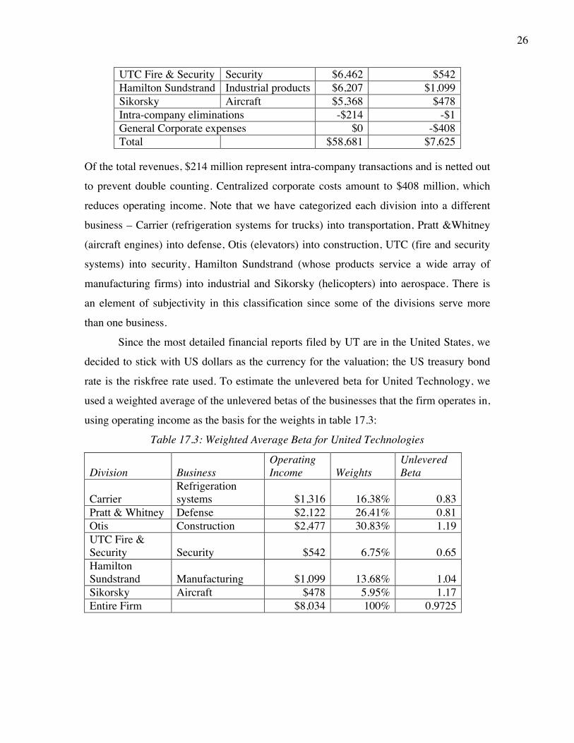
UTC Fire & Security Security $6,462 $542 Hamilton Sundstrand Industrial products $6,207 $1,099 Sikorsky Aircraft $5,368 $478 Intra-company eliminations -$214 -$1 General Corporate expenses $0 -$408 Total $58,681 $7,625

Of the total revenues, $214 million represent intra-company transactions and is netted out

to prevent double counting. Centralized corporate costs amount to $408 million, which

reduces operating income. Note that we have categorized each division into a different

business – Carrier (refrigeration systems for trucks) into transportation, Pratt &Whitney

(aircraft engines) into defense, Otis (elevators) into construction, UTC (fire and security

systems) into security, Hamilton Sundstrand (whose products service a wide array of

manufacturing firms) into industrial and Sikorsky (helicopters) into aerospace. There is

an element of subjectivity in this classification since some of the divisions serve more

than one business.

Since the most detailed financial reports filed by UT are in the United States, we

decided to stick with US dollars as the currency for the valuation; the US treasury bond

rate is the riskfree rate used. To estimate the unlevered beta for United Technology, we

used a weighted average of the unlevered betas of the businesses that the firm operates in,

using operating income as the basis for the weights in table 17.3:

Table 17.3: Weighted Average Beta for United Technologies

Division Business Operating Income Weights

Unlevered Beta

Carrier Refrigeration systems $1,316 16.38% 0.83

Pratt & Whitney Defense $2,122 26.41% 0.81 Otis Construction $2,477 30.83% 1.19 UTC Fire & Security Security $542 6.75% 0.65 Hamilton Sundstrand Manufacturing $1,099 13.68% 1.04 Sikorsky Aircraft $478 5.95% 1.17 Entire Firm $8,034 100% 0.9725

27

To estimate the equity beta for United Technologies, we levered this beta using the

market value of equity and the estimated market value of debt (with lease commitments

treated as debt) in March 2009, and a marginal tax rate of 38%:

Market value of equity = $41,904 million

Estimated market value of debt (including leases)7 = $12,919 million

Levered Beta8 = 0.9725 (1+(1-.38) (11,476/41,904)) = 1.14

United Technologies also has extensive operations outside the United States, with

more than 50% of revenues coming from foreign sales. To estimate the equity risk

premium to use in valuing United Technologies, we estimated a weighted average of

equity risk premiums across operating locations in table 17.4 – using mature market

equity risk premiums of 6.00% in North America and Europe, a 7.80% equity risk

premium for Asia Pacific and 8.40% for revenues from other regions:9

Table 17.4: Equity Risk Premium: United Technologies

Revenues Weight Equity Risk Premium United States $28,234 48.11% 6.00% Europe $15,819 26.96% 6.00% Asia Pacific $8,212 13.99% 7.80% Other $6,416 10.93% 8.40% Company $58,681 100.00% 6.51%

Using the bottom up (levered) beta of 1.14 estimated in the last section, the US treasury

bond rate of 3% as the risk-free rate and the weighted average equity risk premium of

6.51%, we estimated a cost of equity for the consolidated operations of 10.43%:

Cost of equity = 3% + 1.14 (6.51%) = 10.43%

As a final component, we estimated a cost of debt for United Technology, using an

estimated rating of AA for the company and a default spread of 1.75%, reflecting this

rating. The resulting after-tax cost of debt is 2.95%:

7 Conventional debt accounted for $11,476 million; the present value of lease commitments accounts for the rest. 8 Since the unlevered betas were computed using only conventional debt, we used only the conventional debt in levering the beta. 9 Unfortunately, the revenue breakdown provided in UT’s filings are not very informative. Thus, sales from the Asia-Pacific region include sales not only from the emerging markets of Asia (such as India and China) but also from Japan and Australia. There is no breakdown provided of other markets that could include Latin America and Canada. The equity risk premiums for the Asia Pacific and Other regions are estimated by averaging the country risk premiums of countries in each area, using the sizes of the economies as weights.

28

After-tax cost of debt = (Riskfree Rate + Default Spread) (1- Marginal tax rate)

= (3% + 1.75%) (1-.38) = 2.95%

Weighting the costs of debt and equity by their market values generates a cost of capital

of 8.68%.

Cost of capital = 10.43% (41,904/ (41,904+12914)) + 2.95% (12,914/(41,904+12914))

= 8.68%

Since we are valuing the firm on a consolidated basis, we estimated the growth rate in the

aggregated cash flows, using the return on capital for the entire firm and the reinvestment

rate in 2009, both of which we assume will be sustained for the next five years:10

Return on capital =

€

After − tax Operating Incomet

(Book Value of Equity + Book Value of Debt - Cash)t -1

=

€

$5,253(26,736 +10,591- 2904)

=15.26%

Reinvestment Rate =

€

Capital Expenditure - Depreciation + Change in non - cash WCAfter - tax Operating Income

=

€

4939 - 2971 + 1665,253

= 40.62%

Expected growth rate = Reinvestment Rate * Return on invested capital

= .4062* .1526 = 6.20%

We forecast operating income, using 6.20% as the expected growth rate, and estimate the

reinvestment each year, based upon the reinvestment rate of 40.62%, for the next 5 years,

in table 17.5:

Table 17.5: Expected Free Cashflow to Firm (in millions) – United Technologies

Year 1 2 3 4 5 EBIT (1-t) $5,578 $5,924 $6,253 $6,521 $6,717 - Reinvestment $2,266 $2,407 $2,407 $2,233 $2,015 FCFF $3,312 $3,517 $3,846 $4,288 $4,702 PV @ 8.68% $3,048 $2,978 $2,996 $3,073 $3,101

10 When estimating the return on capital and reinvestment rate, we made two adjustments to the stated earnings and book capital numbers. The first was the capitalization of operating leases, which is treated as debt for book capital purposes. The second is the capitalization of R&D expenses for the firm, which increases the book value of equity, and changes the values for both the operating income and capital expenditure numbers. We also included acquisitions of $1,448 million, in 2009, as part of reinvestment, since it is a standard part of United Technologies growth strategy; the firm has done acquisitions every year for the last 4 years.

29

The present value of the cash flows is computed, using the cost of capital of 8.68% that

we estimated earlier; the aggregated present value of the cash flows is $15,196 million.

As the final piece in this valuation, we assume that the firm will be in stable

growth, growing at 3% a year in perpetuity, beyond year 5 and that while its cost of

capital will remain unchanged at the current level (8.68%), it’s return on capital will

decrease to 10%, reflected its larger size and increased competition.

Stable period reinvestment rate =

€

gROC

=.03.10

= .30 or 30%

Terminal value =

€

After - tax Operating Income5 (1 +g) (1- Reinvestment Ratestable)(Cost of capital - gstable)

=

€

6,717 (1.03) (1- .30)(.0868 - .03)

= $85,248 million

Discounting this terminal value back to the present at the current cost of capital and

adding it on the present value of expected cash flows generates a value for the operating

assets of $71,410 million.

Value of operating assets = PV of cash flows during high growth +

€

Terminal Valuen

(1+Cost of capital)n

= $15,198 million +

€

$ 85,248 m(1.0868)5 = $71,410 million

United Technologies has no minority holdings in other firms but it does report minority

interests of $1,009 million on its balance sheet. Since we know that this represents a

subsidiary in the technology business, where firms typically trade at 1.75 times book

value, we estimate a market value for the minority interests.

Minority interestsMarket Value = Minority interestsBook Value * Average P/BV for sector

= $1,009 million * 1.75 = $1,766 million

We subtract this value as well as the value of debt ($12,919), while adding the cash

balance ($ 4,327 million) to estimate the value of equity:

Value of Equity = Value of Operating Assets + Cash – Debt – Value of minority interests

= $71,410 + $4,327 – $12,919- $1,766 = $61,062 million

Subtracting out the estimated value of equity options outstanding (51 million options,

with an average strike price of $40.35, valued at $544 million) and dividing by the

30

number of shares outstanding (942.29 million shares), we estimate a value per share of

$64.22.

Value per share =

€

Value of equity - Value of equity optionsPrimary number of shares

= (61,062 - 544)942.29

= $64.22

The stock was trading at $44.47 at the time of this analysis, making it significantly under

valued.

Illustration 17.2: Valuing United Technologies – Disaggregated Basis

To value United Technologies on a disaggregated basis, we extended our search

for division specific information to include other operating items. Table 17.6 reports on

the breakdown of total assets, capital invested and depreciation across the firm:

Table 17.6: Business Breakdown – United Technologies

Division Business Revenues

Pre-tax Operating Income

Capital Expenditures Depreciation

Total Assets

Carrier Refrigeration systems $14,944 $1,316 $191 $194 $10,810

Pratt & Whitney Defense $12,965 $2,122 $412 $368 $9,650 Otis Construction $12,949 $2,477 $150 $203 $7,731 UTC Fire & Security Security $6,462 $542 $95 $238 $10,022 Hamilton Sundstrand Manufacturing $6,207 $1,099 $141 $178 $8,648 Sikorsky Aircraft $5,368 $478 $165 $62 $3,985

There are two problems that we face in using this information. The first is that the

information that is provided does not quite match up to the information that we need to

value these businesses. Thus, we would have preferred to see capital invested by division,

rather than total assets, and total reinvestment, which would include acquisitions and

working capital, rather than capital invested. The second is that there is some information

that we would like to have that is unavailable. We would, for instance, like to see the

geographical breakdown of revenues within each division and the debt used by each, the

former to estimate equity risk premiums and the latter to compute levered betas and costs

of capital.

31

We first wrestled with the estimation of cost of capital, by division, a process that

requires a debt ratio, by division, and an after-tax cost of debt. Since there is no

breakdown of debt, by division, we considered three options.

• Allocate the total debt of the firm ($12,919 million) across the divisions, using the

total assets as the basis for the allocation. We could then use either the cost of

debt of the company for all the divisions, or attempt to estimate synthetic ratings

and costs of debt for each division. Since we would still need to estimate the

market value of equity in each division, we decided that this choice would create

more problems than solutions, at least for this company.

• Use the average market debt ratio of the publicly traded firms in each business as

the debt ratio for the division. Thus, Otis, being in the construction business,

would have a higher debt to equity ratio than Hamilton Sundstrand, in the

industrial products business. The residual problem of making this choice is that

the debt across the divisions will not add up to the total debt outstanding for the

company. While we could use an allocation mechanism, based upon the industry

debt ratios, the differences in the industry average debt to equity ratios was not

large enough for the process to pay off.

• Use the company’s debt ratio as the debt ratio for all the divisions and the cost of

debt of the company as the cost for each division. While this can lead to skewed

estimates for companies that have businesses that have very different debt

capacity, United Technologies businesses are all capital intensive and profitable,

and it seems reasonable that all of the divisions will carry debt ratios that similar

to the overall company.

Since the geographic breakdown is not provided by division, we will assume that they are

identical to the company’s overall exposure, leading to an equity risk premium of 6.51%

(estimated in the last illustration) for all of the divisions.

In Table 17.7, we summarize our estimates of levered betas and the costs of

equity and capital for the businesses, on the assumption that the debt ratios for all of the

divisions matches the company’s debt ratio of 23.33%:

Table 17.7: Levered Betas and Costs of Equity/Capital by business

Division Unlevered Debt/Equity Levered Cost of After-tax Debt to Cost of

32

Beta Ratio beta equity cost of debt

Capital capital

Carrier 0.83 30.44% 0.97 9.32% 2.95% 23.33% 7.84% Pratt & Whitney 0.81 30.44% 0.95 9.17% 2.95% 23.33% 7.72% Otis 1.19 30.44% 1.39 12.07% 2.95% 23.33% 9.94% UTC Fire & Security 0.65 30.44% 0.76 7.95% 2.95% 23.33% 6.78% Hamilton Sundstrand 1.04 30.44% 1.22 10.93% 2.95% 23.33% 9.06% Sikorsky 1.17 30.44% 1.37 11.92% 2.95% 23.33% 9.82%

Based on our estimates, the costs of capital range from 6.78% for UTC Fire and Security

to 9.94% for Otis.

We allocated the total capital invested in the firm ($28,287 million) across the

businesses, based upon the total assets, and the total reinvestment for the firm in 2009

($2,134 million), based upon the capital expenditures. We used these allocated numbers

as our basis for computing the after-tax return on capital and reinvestment rates, by

division, in table 17.8:

Table 17.8: Return on Capital and Reinvestment Rates by division: United Technologies

Division Total Assets

Capital Invested

Cap Ex

Allocated Reinvestment

Operating income after taxes

Return on capital

Reinvestment Rate

Carrier $10,810 $6,014 $191 $353 $816 13.57% 43.28% Pratt & Whitney $9,650 $5,369 $412 $762 $1,316 24.51% 57.90% Otis $7,731 $4,301 $150 $277 $1,536 35.71% 18.06% UTC Fire & Security $10,022 $5,575 $95 $176 $336 6.03% 52.27% Hamilton Sundstrand $8,648 $4,811 $141 $261 $681 14.16% 38.26% Sikorsky $3,985 $2,217 $165 $305 $296 13.37% 102.95%

aReturn on capital = Operating income after taxes/ Capital invested bReinvestment Rate = Reinvestment/ Operating income after taxes

To estimate the expected growth rate, we assume that these reinvestment rates and returns

on capital can be maintained for the near term. The resulting expected growth rates are

summarized in table 17.9, with the judgments that we made about the growth that will

occur in the future:

Table 17.9: Expected Growth Rates and Growth Pattern Choices

Division Cost of capital

Return on capital

Reinvestment Rate

Expected growth

Length of growth period

Stable growth rate

Stable ROC

Carrier 7.84% 13.57% 43.28% 5.87% 5 3% 7.84%

33

Pratt & Whitney 7.72% 24.51% 57.90% 14.19% 5 3% 12.00% Otis 9.94% 35.71% 18.06% 6.45% 5 3% 14.00% UTC Fire & Security 6.78% 6.03% 52.27% 3.15% 0 3% 6.78% Hamilton Sundstrand 9.06% 14.16% 38.26% 5.42% 5 3% 9.06% Sikorsky 9.82% 13.37% 102.95% 13.76% 5 3% 9.82%

We have assumed that all of the divisions, other than UTC Fire and Security, will be able

to maintain their current returns on capital and reinvestment rates for the next five years.

In stable growth, the growth rate will be 3% for all divisions, with returns on capital

moving to the cost of capital for four of the divisions, but staying above the cost of

capital for the two divisions that have the highest current returns on capital (Pratt &

Whitney and Otis). With UTC Fire and Security, we assume that the firm is already in

stable growth, since its growth rate (3.15%) is close to the stable growth rate (3%) and

that its return on capital will be equal to the cost of capital.

Equipped with these expected growth rates and costs of capital, we first compute

the expected free cash flows, by division, for the high growth phase in table 17.10:

Table 17.10: Expected Free Cash Flow and Present Value- By division

Business EBIT (1-t)

Expected growth rate

Reinvestment Rate 1 2 3 4 5

Present value

Carrier $816 5.87% 43.28% $490 $519 $549 $581 $616 $2,190

Pratt & Whitney $1,316 14.19% 57.90% $632 $722 $825 $942 $1,075 $3,310

Otis $1,536 6.45% 18.06% $1,340 $1,426 $1,518 $1,616 $1,720 $5,717 UTC Fire & Security $336 3.15% 52.27% $0 Hamilton Sundstrand $681 5.42% 38.26% $443 $467 $493 $520 $548 $1,902

Sikorsky $296 13.76% 102.95% -$10 -$11 -$13 -$15 -$17 -$49

Note that there are no high growth cash flows for UTC, since it is assumed to be in stable

growth. We then estimate the value at the end of the high growth phase for each firm in

table 17.11:

Table 17.11: Estimated Terminal Value – By Division

Business

After-tax Operating income

Stable growth rate Stable ROC

Stable Reinvestment Rate

Terminal Value

Carrier $1,085 3% 7.84% 38.28% $13,850 Pratt & Whitney $2,554 3% 12.00% 25.00% $40,593 Otis $2,099 3% 14.00% 21.43% $23,766 UTC Fire & $336 3% 6.78% 44.22% $4,953

34

Security Hamilton Sundstrand $887 3% 9.06% 33.10% $9,788 Sikorsky $565 3% 9.82% 30.54% $5,749

For UTC Fire and Security, the terminal value is the value of the operating assets today.

For the other divisions, the expected cash flows for the next five years and the terminal

value have to be discounted back at the costs of capital we estimated earlier. Table 17.12

summarizes the final estimates of value for operating assets, by division:

Table 17.12: Estimated Operating Asset Value by division

Business Cost of capital

PV of FCFF

PV of Terminal Value

Value of Operating Assets

Carrier 7.84% $2,190 $9,498 $11,688 Pratt & Whitney 7.72% $3,310 $27,989 $31,299 Otis 9.94% $5,717 $14,798 $20,515 UTC Fire & Security 6.78% $0 $4,953 $4,953 Hamilton Sundstrand 9.06% $1,902 $6,343 $8,245 Sikorsky 9.82% -$49 $3,598 $3,550 Sum $80,250

Finally, we have to deal with general corporate expense of $408 million, reported by the

firm in 2008, that reduces the overall operating income of the firm. We assume that this

expense, adjusted for taxes, will continue to grow at the stable growth rate of 3%, in

perpetuity. Using the firm’s overall cost of capital of 8.68% as the discount rate, we

estimate the present value of corporate expenses in perpetuity of $ 4.587 billion:

Value of Corporate Expenses =

€

Corporate ExpensesCurrent (1− t)(1+ g)(Cost of capitalCompany − g)

=

€

408(1− .38)(1.03)(.0868 − .03)

= $4,587 million

Reducing the cumulative value of the operating assets from table 17.12 ($80,250

million), by this amount ($4,587 million), generates a value for the operating assets of the

firm of $75,663 million. This is about 6% higher than the value that we obtained for the

operating assets in the last illustration, where we valued United Technologies on an

aggregated basis, of $71,420 million.

35

Relative Valuation

There are two ways in which we can adapt relative valuation to the complex

companies that we have examined in this chapter. The first is to accept the reality that we

will never find comparable firms, defined in terms of business mix, and to focus on either

finding firms that have similar cash flow, growth and risk characteristics or controlling

for differences on those dimensions. The second is an extension of the sum-of-the-parts

relative valuation we described earlier in the chapter, with more attention paid to

adjusting for the characteristics of complex companies.

Extended Relative Valuation

In most relative valuations, analysts stay within a sector to make their valuation

judgments. Thus, a software company is compared to other software companies and a

steel company to other steel companies. Implicitly, we are assuming that firms within a

sector share enough risk, growth and cash flow characteristics to be priced similarly.

When a company operates in many different sectors or businesses, this type of relative

valuation becomes much more difficult to do, since. However, there is no reason why we

cannot expand our relative valuation sample to include firms that are dissimilar from the

one that we are valuing, as long as we control for differences in valuation fundamentals

when we make our comparisons.

In practical terms, we can try to modify the multiples that we use for

fundamentals (as is the case when we use PEG ratios) or use regressions that explicitly

adjust for differences across companies. In January 2009, for instance, a regression of

Price to Book ratios of the 100 largest market cap companies in the United States, against

return on equity, beta and expected growth in earnings per share (over the next 5 years)

yielded the following output:

P/BV = 1.57 + 7.67 ROE + 8.91 Expected growth in EPS -1.64 Beta R2=62%

(3.83) (8.67) (5.63) (5.22)

If we wanted to value GE, a company with almost no directly comparable firms, we

would plug in the values of the independent variables for GE (ROE = 11%, Beta = 1.05,

Expected growth= 7%) into this regression to get a predicted Price to Book Value

multiple for GE:

36

P/BVGE = 1.57 + 7.67 (.11) + 8.91 (.07) -1.64 (1.05) = 1.32

At the time of this analysis, GE was trading at $11.12/share and had a book value of

equity per share of $9.93, resulting in a price to book ratio of 1.12, thus making it under

valued by about 20%.

Modified Sum-of-the-parts Valuation

Earlier in this chapter, we described how some analysts value companies that

operate in multiple businesses, by applying multiples to the earnings or revenues

generated by each business. While there are significant limitations in how they use the

approach, it can be adapted effectively, if we go through three steps:

Step 1: Estimate operating numbers, by business and by region: The first step is to obtain

the operating numbers, by business or region. While many companies provide this

breakdown in their financial statements at least for the key numbers, it is better to steer

away from numbers that are distorted by allocation judgments that are often arbitrary or

tax considerations. Thus, the revenues or EBITDA, reported by business, will generally

be a more reliable base for relative valuation than the net income broken down by

business.

Step 2: Find comparable companies, by business and by region: Once we have the

operating numbers broken down by business and region, we can revert back to the

conventional practices in relative valuation. We can look for publicly traded companies

that operate only or primarily in each business and obtain their market values. If we are

unable to find publicly traded firms in a specific business, we may have to consolidate the

businesses until we do. As an example, if we break GE down into the 25 or 30 different

businesses that it operates in, there may be some businesses where there are no

comparable firms. Dividing GE up into five or six primary businesses will give us a

better shot of finding comparable companies.

Step 3: Estimate relative value, by business and region, controlling for differences in risk

and growth: In this part of the process, we decide on a multiple to use and compute the

summary statistics for the comparable firms. While we can just use the median or

average multiple to estimate the value of each business, a sounder approach would be to

adjust the number for fundamental differences between the firms and the business being

37

valued. It is also worth noting that we can choose different multiples for different

businesses, within the same company. In valuing GE, for instance, we may decide to use

the PE ratio to value GE Capital, since it is in the financial service business, and

EV/EBITDA to value the aircraft engines business, because of its dependence of

infrastructure investment.

Step 4: Estimate the consolidated value: Once we have valued the pieces of the company

separately, we have to aggregate the values. When doing so, though, we have to consider

what the relative values are measuring. In the GE example in the last step, we will obtain

the value of the equity in GE Capital when we use the PE ratio to value it and the value of

the operating assets in GE Aircraft, when we use the EV/EBITDA as our valuation

metric. The former is already an equity value, whereas we need to add cash and subtract

out debt from the latter to get to equity value. If we are using a mix of equity and

enterprise value multiples, it is safest to estimate the equity value in each business and

then aggregate the equity values but that requires us to have a measure of the debt

outstanding and cash holdings of each business.

Step 5: Check for loose ends: Once we have valued the consolidated company, by adding

together the values of the individual businesses, we have two final checks that we need to

run.

• The first is for any unallocated costs (centralized G&A, for instance) that we have not

incorporated into our valuation, which will be the case, if we use revenues or earnings

prior to allocations to value individual businesses. We can adjust the consolidated

value for these costs in one of two ways. The first is look at the costs as a proportion

of after-tax operating income (for the entire firm) and to reduce the value by that

same amount; thus, if centralized costs amount to $ 2 billion on after-tax operating

income of $ 20 billion, we would reduce the consolidated value by 10%. The second

is to apply a multiple to the consolidated costs themselves to arrive at a value; one

simple way to derive this multiple is to look at the value that we are estimating for the

rest of the company and the multiple of operating income that it represents.

• The second adjustment is for cross holdings, since the way they are accounted for can

distort the values we obtain from relative valuation. The adjustments we make for

minority holdings mirror the ones we made to intrinsic value; we have to estimate the

38

value of these holdings and add that value on to the consolidated value. With majority

holdings, the income reported by business is the consolidated income, we have to

subtract out the estimated value of minority interests. If it is just parent company

income, we have to value the majority holdings separately and add them on to

consolidated value.

Illustration 17.3: Sum-of-the-parts Relative Valuation of United Technologies

In illustrations 17.1 and 17.2, we valued United Technologies, using discounted

cash flow models. To value the company, on a relative valuation basis, we will begin

with breakdown, of revenues, EBITDA, operating income and capital invested, by

business, in table 17.13:

Table 17.13: Scaling Variables – By Division

Division Business Revenues EBITDA Operating Income

Capital Invested

Carrier Refrigeration systems $14,944 $1,510 $1,316 $6,014

Pratt & Whitney Defense $12,965 $2,490 $2,122 $5,369 Otis Construction $12,949 $2,680 $2,477 $4,301 UTC Fire & Security Security $6,462 $780 $542 $5,575 Hamilton Sundstrand Industrial Products $6,207 $1,277 $1,099 $4,811 Sikorsky Aircraft $5,368 $540 $478 $2,217 Total $58,895 $9,277 $8,034 $28,287

Thus, our choices on multiples are narrowed to one of these four variables, with

enterprise value (rather than equity value) being estimated. To decide which multiple

(EV/Revenues, EV/EBITDA, EV/EBIT or EV/Capital) to use in the valuation, we looked

at the publicly traded companies within each business and tried to explain differences

across companies (within each business) using all four multiples. We then chose the

multiple that had the most significant explanatory power (highest R-squared on the sector

regression) for each business. Table 17.14 summarizes the multiple used, by business,

and the regression equation that generated the statistical significance:

Table 17.14: Choosing a Multiple – Business

Business Best Multiple Regression R2

Refrigeration systems EV/EBITDA EV/EBITDA = 5.35 – 3.55 Tax Rate + 14.17 ROC

42%

Defense EV/Revenues EV/Revenues = 0.85 + 7.32 Pre-tax Operating Margin 47%

39

Construction EV/EBITDA EV/EBITDA = 3.17 – 2.87 Tax Rate + 14.66 ROC 36% Security EV/Capital EV/ Capital = 0.55 + 8.22 ROC 55% Industrial Products EV/Revenues EV/Revenues = 0.51 + 6.13 Pre-tax Operating Margin

48%

Aircraft EV/Capital EV/ Capital = 0.65 + 6.98 ROC 40%

Finally, we used the multiple chosen in each business, in conjunction with the sector

regression, to estimate a value for each of United Technologies different businesses in

table 17.15:

Table 17.15: Estimated Relative Value – By Business

Division Scaling Variable

Current value for scaling variable ROC

Operating Margin

Tax Rate Predicted Multiple

Estimated Value

Carrier EBITDA $1,510 13.57% 8.81% 38% 5.35 – 3.55 (.38) + 14.17 (.1357) =5.92 $8,944.47

Pratt & Whitney Revenues $12,965 24.51% 16.37% 38%

0.85 + 7.32 (.1637) =2.05 $26,553.29

Otis EBITDA $2,680 35.71% 19.13% 38%

3.17 – 2.87 (.38)+14.66 (.3571) =7.31 $19,601.70

UTC Fire & Security Capital $5,575 6.03% 8.39% 38%

0.55 + 8.22 (.0603) =1.05 $5,828.76

Hamilton Sundstrand Revenues $6,207 14.16% 17.71% 38%

0.51 + 6.13 (.1771) =1.59 $9,902.44

Sikorsky Capital $2,217 13.37% 8.90% 38% 0.65 + 6.98 (.1337) =1.58 $3,509.61

$74,230.37

As with the disaggregated discounted cash flow valuation, we have to deal with corporate

expenses of $ 408 million and we have two choices. One is to use a discounted cash flow

approach to estimate the value; this yielded $4,587 million in illustration 17.*. The other

is to stay within a relative valuation framework and apply a multiple to this expense. In

fact, the value ($74,230) that we have estimated for the operating divisions of United in

table 17.15 is about 9.25 times the cumulated operating income ($8,034 million) across

the divisions. Applying this multiple to the corporate expenses results in a capitalized

value of about $3,775 million, which when subtracted from the overall value, yields a

value for the operating assets of $70,565 million, a little lower than the values that we

estimated using the intrinsic value approaches. Note that the rest of the adjustments

(adding cash, subtracting debt and minority interests and adjusting for options

outstanding) still have to be made to derive equity value per share.

40

Conclusion Companies that spread their tentacles across multiple business and many parts of

the globe are difficult to value, because their cash flows from each business or region can

have very different risk and growth characteristics. In this chapter, we looked at two ways

that we can approach the valuation of these. The first is to value the company as a whole,

using the weighted averages of risk parameters to estimate discount rates, which we then

use to discount consolidated cash flows for the firm. The dangers here are that the

weights will change over time, and as they do, so will the fundamentals of the firm. The

second is to value the cash flow streams separately, using different risk measures and

growth rates for each stream. Thus, emerging market and risky business cash flows will

be discounted at higher rates than developed market and safer business cash flows. The

aggregated value of the different businesses should yield a better estimate of the overall

company’s value.

When we use relative valuation to value these companies, we run into the same

valuation issues. Again, we can try to value the consolidated firm, but finding companies

that are similar in business mix is an almost impossible task. For that reason, it makes

sense to expand our definition of comparable firms to include firms that may not be

similar to the multi-business firm that we are valuing, and to control for differences on

valuation fundamentals – risk, cash flow and growth. Alternatively, we can try to find

comparable firms within each business, and use the information in how the market is

pricing these companies to value the pieces that make up the larger firm.

No matter what approach we use, we will be faced with more complexity and

information gaps with multi-business companies than with single business, independent

companies. We have to determine whether this complexity exposes us to more risk and, if

so, how we will incorporate that concern into value.